Learning to Learn Financial Networks for Optimising Momentum Strategies

Abstract.

Network momentum provides a novel type of risk premium, which exploits the interconnections among assets in a financial network to predict future returns. However, the current process of constructing financial networks relies heavily on expensive databases and financial expertise, limiting accessibility for small-sized and academic institutions. Furthermore, the traditional approach treats network construction and portfolio optimisation as separate tasks, potentially hindering optimal portfolio performance. To address these challenges, we propose L2GMOM, an end-to-end machine learning framework that simultaneously learns financial networks and optimises trading signals for network momentum strategies. The model of L2GMOM is a neural network with a highly interpretable forward propagation architecture, which is derived from algorithm unrolling. The L2GMOM is flexible and can be trained with diverse loss functions for portfolio performance, e.g. the negative Sharpe ratio. Backtesting on 64 continuous future contracts demonstrates a significant improvement in portfolio profitability and risk control, with a Sharpe ratio of 1.74 across a 20-year period.

1. Introduction

Financial networks represent interconnections among financial entities such as institutions, markets and assets, and are constructed to facilitate the analysis of various downstream tasks. These tasks primarily focus on systemic risk assessment and market structure analysis, and more recently on alpha research and portfolio optimisation (Ali and Hirshleifer, 2020; Lee et al., 2019). Network momentum is a type of network alpha signals, which is based on the idea that the future return of one company in the financial network can be predicted from the past returns of companies to which it is connected, a phenomenon known as momentum spillover (Ali and Hirshleifer, 2020).

The construction of financial networks is crucial to the success of network momentum signals. Nodes often represent individual stocks, while edges capture the relations between them and are constructed based on various financial or economic factors. These factors include, but are not limited to, industry or business similarity (Moskowitz and Grinblatt, 1999; Boni and Womack, 2006), geographical proximity (Parsons et al., 2020; Korniotis and Kumar, 2013) news co-mentions (Wan et al., 2021) and supply-demand links (Cohen and Frazzini, 2008; Menzly and Ozbas, 2010). However, the construction of these networks often relies on acquiring expensive databases from domain experts with deep understanding of finance and economics, making it costly for small-sized, non-profit or academic institutions. Alternatively, we may adopt the reasonable assumption that momentum spillover is subtly echoed in the historical pricing data, which are more readily accessible. Therefore, if an effective model could be developed to learn the relationship between companies from readily available data, it could significantly lessen the dependence on costly data acquisition and specialised financial knowledge. Nevertheless, creating such a model remains a significant open challenge in the field of machine learning and quantitative finance.

Another limitation of the literature is that the construction of financial networks or graphs is often detached from the subsequent downstream tasks. For example, analysts tend to focus more on economic justification when constructing these graphs, giving less consideration to whether they would lead to optimal portfolio performance. However, it is possible that the method of graph construction, such as deducing a custom sales ratio formula to determine the connection strength between two companies (Cohen and Frazzini, 2008), may not help with achieving optimal portfolio performance. In other words, the graph may not be effectively optimised with respect to portfolio performance. This underscores the need for a task-specific graph construction framework.

In response to these considerations, we propose an end-to-end machine learning framework capable of simultaneously learning financial graphs and optimising the trading signals from momentum features built from these networks. Our framework leverages the concept of learning to learn graph topologies (L2G) (Pu et al., 2021). Traditional graph learning methods typically employ convex optimisation to solve for an optimal graph given observed data on nodes (Dong et al., 2019, 2016). L2G reformulated this process into learning a parametric mapping, where node features are input and the graph serves as the output, by unrolling the optimisation algorithm into a forward propagation of a neural network. Taking advantage of the flexibility in neural architecture design and training, we propose to incorporate into L2G an additional layer for constructing network momentum features, and train the model with loss being portfolio performance metrics in an end-to-end fashion.

We test the proposed strategy, Learning to Learn Financial Networks for Optimising Momentum Strategies (L2GMOM), on 64 continuous future contracts, spanning commodities, equities, fixed income funds, and foreign currencies. We obtain a Sharpe ratio of 1.74 across 20-year backtest period from 2000 to 2020 (Baz et al., 2015; Lim et al., 2019). In addition, the learned financial graphs effectively elucidate the momentum spillover for portfolio construction, which enhances the interpretability of the proposed methods. Our model also excels in terms of computational efficiency, offering rapid inference in milliseconds and bypassing the need for daily graph optimisation.

The major contributions of our work are threefold: Firstly, we present a novel methodology that uses easily accessible pricing data to infer financial networks between assets. This approach eliminates the costly requirement for alternative datasets and reduces human bias. Secondly, we propose an end-to-end learning framework that is capable of both inferring financial networks and simultaneously optimising the downstream task of portfolio construction. This ensures the financial networks are directly optimised in relation to portfolio performance. Finally, our proposed methods demonstrate strong empirical portfolio performance in both profitability and risk control.

2. Preliminary

2.1. Individual Momentum Strategy

The concept of individual asset momentum, proposed by (Moskowitz and Grinblatt, 1999), explores the profitability by longing past winner assets and shorting past underperformers. A time-series (TSMOM) momentum can be therefore constructed, with the daily return defined as

(1) $$r_{t:t+1}^{\text{portfolio}}:=\frac{1}{N_{t}}\sum_{i=1}^{N_{t}}x_{i,t}\frac{\sigma_{\text{tgt}}}{\sigma_{i,t}}r_{i,t:t+1}$$

where $N_{t}$ is the number of assets at day $t$, $r_{i,t:t+1}$ is the daily return of asset $i$. With the target annualised volatility $\sigma_{\text{tgt}}$, the asset return is scaled by its annualised realised volatility $\sigma_{i,t}$. Here, $\sigma_{\text{tgt}}=0.15$ following literature standards (Lim et al., 2019), and $\sigma_{i,t}$ is estimated from an exponential weighted moving standard deviation with a 60-day span on daily returns. The position, or trading signal $x_{i,t}\in[-1,1]$ at day $t$ for asset $i$, specifies the strategy. The core of momentum strategies is the construction of the trading signal $x_{i,t}$. It often consists of two steps - trend estimation and position sizing. We illustrate this with the following examples.

Annual Return

Moskowitz et al. (2012) proposed to use past 1-year asset return $r_{i,t-252:t}$ as a trend estimation, and the direction as the position $x_{i,t}=\text{sgn}(r_{i,t-252:t})$.

MACD

Baz et al. (2015) constructed trend estimation using the volatility normalised moving average crossover divergence (MACD) indicators such that

(2) $$\text{MACD}(i,t,S,L)=m(i,t,S)-m(i,t,L)$$

(3) $$\text{MACD}_{\text{norm}}(i,t,S,L)=\frac{\text{MACD}(i,t,S,L)}{\text{std}(p_{i,t-63:t})}$$

(4) $$y_{i,t}(S,L)=\frac{\text{MACD}_{\text{norm}}(i,t,S,L)}{\text{std}(\text{MACD}_{\text{norm}}(i,t-252,S,L))}$$

(5) $$x_{i,t}=\frac{1}{3}\sum_{k=1}^{3}\phi(y_{i,t}(S_{k},L_{k}))$$

where $(S_{k},L_{k})\in\{(8,24),(16,48),(32,96)\}$ and $\phi(y)=\frac{y\exp(-y^{2}/4)}{0.89}$ is a position scaling function.

Machine Learning-based TSMOM

Recent literature managed to construct TSMOM from machine learning models. Lim et al. (2019) proposed a general supervised learning framework such that

(6) $$x_{i,t}=\text{sgn}(y_{i,t})\quad\text{and}\quad y_{i,t}=f_{\boldsymbol{\theta}}(\mathbf{u}_{i,t}).$$

It can also directly model the position:

(7) $$x_{i,t}=f_{\boldsymbol{\theta}}(\mathbf{u}_{i,t})$$

The model specifications for $f$ are diverse and often considered in relation to the nature of the input feature $\mathbf{u}$. Lim et al. (2019) compared linear models and deep learning models, such as Lasso Regression, MLP, WaveNet, and LSTM, using input features such as the MACD indicators and volatility-scaled returns from diverse lookback windows. In a similar vein, Wood et al. (2022) considered an attention-based deep learning model. Tan et al. (2023) and Liu et al. (2023) proposed advanced deep learning to effectively model for time-series and cross-sectional momentum.

2.2. Network Momentum Strategy

Network momentum strategy takes into account the interconnections of assets, assuming an asset’s future performance can be influenced by the past performance of its linked assets. A network or graph is defined to represent economic links between assets, modelled by a graph adjacency matrix $\mathbf{A}_{t}$ at time $t$. A general framework of network momentum strategies starts by defining a network or graph to represent certain economic links between two assets. The network is mathematically modelled by a graph adjacency matrix $\mathbf{A}_{t}\in\mathbb{R}^{N_{t}\times N_{t}}$ between $N_{t}$ assets at time $t$, where the entries $a_{ii,t}=0$ and $a_{ij,t}\geq 0$. If $a_{ij,t}>0$, there exists an economic link that shows certain similarity between asset $i$ and asset $j$. Some studies (Moskowitz and Grinblatt, 1999; Boni and Womack, 2006) defined binary graph such that $a_{ij,t}\in\{0,1\}$, while others (Yamamoto et al., 2021; Ali and Hirshleifer, 2020) also quantified the strength of the interconnections using edge weights.

The network momentum of asset $i$ at time $t$ is defined through the average of trend estimation propagated from its connected assets in $\mathbf{A}_{t}$:

(8) $$y_{i,t}=\frac{1}{|\mathcal{N}_{t}(i)|}\sum_{j\in\mathcal{N}_{t}(i)}a_{ij,t}y_{j,t}$$

where $\mathcal{N}_{t}(i)$ is the neighbourhood set of asset $i$ at time $t$ containing all its connected assets. In the literature, different economic links were explored. Some examples of $\mathbf{A}$ include:

• Industry Linkage. $a_{ij,t}=1$ if stock $i$ and $j$ belong to the same industry, based on industrial classification codes such as two-digit SIC (Moskowitz and Grinblatt, 1999) and GICS (Boni and Womack, 2006).

• Supply-demand Relations (Menzly and Ozbas, 2010; Yamamoto et al., 2021). Cohen and Frazzini (2008) define a customer link $a_{ij,t}=1$ for a target firm $i$ if it sells more then 10% its products or services to the firm $j$.

• Geographic Location. $a_{ij,t}=1$ if two companies have headquarters in the same location (Parsons et al., 2020; Korniotis and Kumar, 2013).

• Patent Similarity. Lee et al. (2019) define a technology proximity score $a_{ij,t}$ to measure the similarity of patent portfolios between two firms.

• Analyst co-coverage. Ali and Hirshleifer (2020) defined $a_{ij,t}$ as the number of sell-side analysts who cover stock $i$ and $j$ in the same report at time $t$.

While the above networks can effectively capture some economic similarity between companies and potentially generate alpha signals, they often rely on expensive databases from domain experts with deep understanding of finance. In this paper, we propose learning the graph adjacency matrix $\mathbf{A}_{t}$ from readily accessible historical returns that directly optimises momentum strategy.

2.3. Learning to Learn Graph Topologies

Graph learning involves estimating a graph adjacency matrix by exploring the spectral characteristics presented in the node observations (Dong et al., 2019; Kalofolias, 2016; Dong et al., 2016; Mateos et al., 2019). Given a feature matrix $\mathbf{V}\in\mathbb{R}^{N\times F}$ on $N$ nodes, the graph adjacency matrix can be optimised for by solving a convex optimisation problem such as the one in (Kalofolias, 2016):

(9) $$\min_{\mathbf{A}} ~{}~{}\text{tr}\Big{(}\mathbf{V}^{\top}(\mathbf{D}-\mathbf{A})\mathbf{V}\Big{)}-\alpha\mathbf{1}^{\top}\log(\mathbf{A}\mathbf{1})+\beta||\mathbf{A}||_{F}^{2}$$

$$s.t. ~{}~{}\mathbf{A}_{ij}=\mathbf{A}_{ji},~{}~{}\mathbf{A}_{ij}\geq 0~{}~{}\forall i\neq j$$

where $\mathbf{D}$ is a diagonal matrix with $\mathbf{D}_{ii}=\sum_{j}\mathbf{A}_{ij}$. The first trace term measures the spectral variations of $\mathbf{V}$ on the learned graph, encouraging connections between nodes with similar features. The log and $\ell_{2}$ terms act as topological regularisation in the optimisation problem, enforcing graph connectivity to avoid isolated nodes and ensure a smooth edge weight distribution. The constraints ensure the learned graph adjacency matrix is symmetric and non-negative.

Although the optimisation problem can be efficiently solved by proximal gradient descent algorithms like primal-dual splitting (PDS), choices of hyperparameters $\alpha$ and $\beta$, significantly influence the resulting graph’s topological structure, such as its sparsity. To address this, Pu et al. (2021) introduced Learning to Learn Graph Topologies (L2G), a method reformulating the optimisation problem into a task of learning a parametric mapping. A neural network with a forward propagation step is proposed by unrolling the iterative PDS optimisation steps (as in Algorithm 1). The hyperparameters that influence the graph’s topological characteristics transform into learnable parameters, which are trained using a loss function comparing graph estimates against ground truth graphs.

In our context, each financial asset represents a node, and their historical pricing data act as node observations. With graph learning, we can reveal the interconnections between assets. Learning to Learn Graph Topologies (L2G) provides further inspiration, as we can now use a loss function associated with portfolio performance to determine the optimal graph structure.

3. Proposed Methodology

3.1. L2GMOM

In this section, we introduce Learning to Learn Financial Networks for Optimising Momentum Strategies (L2GMOM), a solution specifically designed to learn financial networks from readily available data and optimise them directly for an ideal portfolio performance.

As introduced in Section 2.3, L2G reformulates optimisation-based graph learning into an unrolling neural network. By leveraging the inherent modularity of neural networks, where different layers can be easily stacked for forward propagation, we propose to incorporate an additional layer into L2G for directly constructing network momentum. Given a feature matrix $\mathbf{V}_{t}$ captured from $N_{t}$ assets at time $t$, the initial step of L2GMOM involves employing the L2G layer (Algorithm 1), as defined in Eq.(10a), to learn a graph adjacency matrix $\mathbf{A}_{t}$. This matrix illustrates the interconnections among the assets. Subsequently, $\mathbf{A}_{t}$ has a normalisation step, as outlined in Eq.(10b). The normalisation aims to offset the dominance of nodes with many connections. In line with the machine learning-based TSMOM approach (Lim et al., 2019) and traditional network momentum in Eq.(8), we propose a linear layer to estimate the momentum trend of asset $i$, derived from a linear combination of individual momentum features $\mathbf{U}_{t}$ of its connected assets in $\tilde{\mathbf{A}}_{t}$. $\tilde{\mathbf{A}}_{t}\mathbf{U}_{t}$ has an interpretation of a network momentum features and the learned parameters $\boldsymbol{\theta}$ are the weights of combining different momentum features. It is worth mentioning that $\tilde{\mathbf{A}}_{t}$ from Eq.(10b) contains only non-negative edges, as a result of enforcing the constraints of Eq.(9). In summary, these are the forward propagation rules for the L2GMOM neural network:

(10a) $$\mathbf{A}_{t}=\textbf{L2G}(\mathbf{V}_{t},L;~{}\boldsymbol{\alpha},\boldsymbol{\beta},\boldsymbol{\gamma})$$

(10b) $$\tilde{\mathbf{A}}_{t}=\mathbf{D}_{t}^{-1/2}\mathbf{A}_{t}\mathbf{D}_{t}^{-1/2},~{}\text{where}~{}\mathbf{D}_{ii,t}=\sum_{j}\mathbf{A}_{ij,t},~{}\mathbf{D}_{ij,t}=0$$

(10c) $$(\textbf{L2GMOM})\quad\mathbf{y}_{t}=\tilde{\mathbf{A}}_{t}\mathbf{U}_{t}\boldsymbol{\theta}+b$$

where $\mathbf{y}_{t}$ is the model output, a $N_{t}$-dimensional vector of trend estimations for every assets, such that $\mathbf{y}_{t}=[y_{1,t},y_{2,t},\dots,y_{N_{t},t}]^{T}$. We further take the trading positions $\mathbf{x}_{t}=\text{sgn}(\mathbf{y}_{t})$ for constructing a network momentum strategy. The trainable parameters include $(\boldsymbol{\alpha},\boldsymbol{\beta},\boldsymbol{\gamma},\boldsymbol{\theta},b)$.

Algorithm 1 L2G (PDS unrolling)

0:  Feature matrix $\mathbf{V}\in\mathbb{R}^{N\times F}$, number of unrolling times $L$

1:  Initial primal $\mathbf{w}_{0}=\mathbf{0}\in\mathbb{R}^{N(N-1)/2}$ and dual $\mathbf{v}_{0}=\mathbf{0}\in\mathbb{R}^{N}$

2:  $\mathbf{h}=\text{vech}(\mathbf{H})$, where $\mathbf{H}_{ij}=||\mathbf{V}_{i,:}-\mathbf{V}_{j,:}||^{2}_{2}$

3:  Degree operator $\mathbf{D}$ such that $\mathbf{Dw}=[d_{1},\dots,d_{N}]^{T}$, where $d_{i}=\sum_{j}{\mathbf{W}_{ij}}$ and $\mathbf{w}=\text{vech}(\mathbf{W})$

4:  for $l=0,1,\dots,L$ do

5:     $\mathbf{r}_{1,l}=\mathbf{w}_{l}-\gamma_{l}(2\beta_{l}\mathbf{w}_{l}+2\mathbf{h}+\mathbf{D}^{T}\mathbf{v}_{l})$

6:     $\mathbf{r}_{2,l}=\mathbf{v}_{l}+\gamma_{l}\mathbf{D}\mathbf{w}_{l}$

7:     $\mathbf{p}_{1,l}=\max\{\mathbf{0},\mathbf{r}_{1,l}\}$

8:     $\mathbf{p}_{2,l}=\big{(}\mathbf{r}_{2,l}-\sqrt{\mathbf{r}_{2,l}^{2}+4\alpha_{l}\gamma_{l}}\big{)}/2$

9:     $\mathbf{q}_{1,l}=\mathbf{p}_{1,l}-\gamma_{l}(2\beta_{l}\mathbf{p}_{1,l}+2\mathbf{h}+\mathbf{D}^{T}\mathbf{p}_{2,l})$

10:     $\mathbf{q}_{2,l}=\mathbf{p}_{2,l}+\gamma_{l}\mathbf{D}\mathbf{p}_{1,l}$

11:     $\mathbf{w}_{l+1}=\mathbf{w}_{l}-\mathbf{r}_{1,l}+\mathbf{q}_{1,l}$

12:     $\mathbf{v}_{l+1}=\mathbf{v}_{l}-\mathbf{r}_{2,l}+\mathbf{q}_{2,l}$

13:  end for

14:  return  Graph estimate $\mathbf{A}$ such that $\mathbf{w}_{L}=\text{vech}(\mathbf{A})$

Taking one step further, we also model the direct position $\mathbf{x}_{t}$ instead of the trend estimation $\mathbf{y}_{t}$. We name the model L2GMOM_SR, since we further use Sharpe Ratio (SR) to optimise for the positions, which are consistent with the literature (Lim et al., 2019). Since the resulting positions $\mathbf{x}_{t}$ lie within the range of $[-1,1]$ in TSMOM, we simply introduce a non-linear activation function, tanh, in the linear layer to ensure the same bahaviour:

(11) $$(\textbf{L2GMOM\_SR})\quad\mathbf{x}_{t}=\text{tanh}\Big{(}\tilde{\mathbf{A}}_{t}\mathbf{V}_{t}\boldsymbol{\theta}+b\Big{)}$$

The use of L2GMOM_SR showcases our model’s flexibility, accommodating different loss functions. L2GMOM_SR not only optimises the portfolio positions, but also the graph learning layer, ensuring the network is well optimised w.r.t. Sharpe ratio.

3.2. Input Features

We consider the following eight momentum features calculated from pricing data for $\textbf{U}_{t}$:

• Volatility normalised returns over the past 1-day, 1-month, 3-month, 6-month and 1-year periods; defined as ${}^{r_{t-\Delta:t}}\!/_{\sigma_{t}\sqrt{\Delta}}$, where $\sigma_{t}$ is an ex-ante daily volatility estimated from an exponential weighted moving standard deviation with 60-day span on daily return.

• MACD indicators with three combinations of short and long time scales $(S_{k},L_{k})\in\{(8,24),(16,48),(32,96)\}$ in Eq.(4).

Therefore, $\mathbf{U}_{t}\in\mathbb{R}^{N_{t}\times 8}$ is the matrix containing these eight features for every asset.

For $\textbf{V}_{t}$, we adopt a 252-day lookback window and stack the individual features together. This is to ensure the L2G layer can capture a stable similarity from longer time-series, providing a robust foundation for learning. As a result, we obtain a representation $\mathbf{V}_{t}\in\mathbb{R}^{N_{t}\times 8\delta}$, where $\delta=252$.

In order to mitigate the influence of outliers, we also winsorise the data by capping/flooring it to be within 5 times its exponentially weighted moving (EWM) standard deviations from its EWM average – computed using a 252-day half-life, as adopted by Lim et al. (2019).

3.3. Loss Functions

The parameters in L2GMOM to be estimated include graph learning parameters $(\boldsymbol{\alpha},\boldsymbol{\beta},\boldsymbol{\gamma})$ and momentum feature parameters $(\boldsymbol{\theta},b)$. Note that Pu et al. (2021) observed that allowing varying hyperparameters $(\alpha,\beta,\gamma)$ in each unrolling layer would significantly increase the performance of graph learning. Therefore, we adopt the same approach. The coefficients are learned by minimising with respect to different loss functions associated with portfolio performance, depending on whether the output is $\mathbf{y}_{t}$ or $\mathbf{x}_{t}$.

• Mean Squared Error (MSE) for training L2GMOM:

  (12) $$\mathcal{L}_{\text{MSE}}(\boldsymbol{\theta},b)=\frac{1}{|\Omega|}\sum_{(i,t)\in\Omega}\left(y_{i,t}-\frac{r_{i,t:t+1}}{\sigma_{i,t}}\right)^{2}$$

• Negative Sharpe Ratio for training L2GMOM_SR:

  (13) $$\mathcal{L}_{\text{SR}}(\boldsymbol{\theta},b)=-\frac{\sum_{(i,t)\in\Omega}R_{i,t}\times\sqrt{252}}{\sum_{(i,t)\in\Omega}R_{i,t}^{2}-(\sum_{(i,t)\in\Omega}R_{i,t})^{2}}$$

  where $R_{i,t}=x_{i,t}\frac{\sigma_{\text{tgt}}}{\sigma_{i,t}}r_{i,t:t+1}$ is the volatility-normalised return of asset $i$ at time $t$.

4. Performance Evaluation

4.1. Backtest Setup

4.1.1. Datasets

Our dataset contains 64 ratio-adjusted continuous future contracts obtained from the Pinnacle Data Crop CLC Database. We computed the momentum feature in Section 3.2 from the daily prices from 1990 to 2020, although different assets could have different time spans when the prices are available. In Appendix, Table 2 lists all the assets used in backtest.

4.1.2. Strategy Candidates

We compare the proposed strategies against the following reference benchmarks:

• Long Only takes a consistent long position $x_{i,t}=1$ with daily volatility scaling in Eq.(1)

• MACD (Baz et al., 2015) takes positions from Eq.(5).

• LinReg (Lim et al., 2019) stands for Linear Regression with the eight momentum features as covariates, and the signals were constructed following Eq.(6) .

• GLinReg stands for Graph Linear Regression. We learn graphs separately with Eq.(9) and we fit them in Eq.(10c). This is to demonstrate whether the performance gain is from the end-to-end learning architecture.

We name the strategies constructed from the proposed models as L2GMOM and L2GMOM_SR. The positions of L2GMOM are the signs of the trend estimation in Eq.(10c), and L2GMOM_SR directly outputs the positions.

4.1.3. Optimisation Details

The models were trained every 5 years, involving coefficient optimisation and hyperparameter tuning using data up to the re-trained time point. These optimised models were then used to generate trading signals for the subsequent 5 years, using out-of-sample data. To ensure an adequate number of training samples, the first backtest period covered 1990-1999 for training and 2000-2004 for testing. Similarly, the second period included 1990-2004 for training and 2005-2009 for testing, and so on. Thus, we had a 20-year aggregated out-of-sample period from 2000 to 2020. For each backtest period, the most recent 10% of training data was set aside as a validation set for hyperparameter tuning. The hyperparameters included the number of unrolling times $L$ in Algorithm 1, batch size, and optimiser parameters. Linear models such as LinReg and GLinReg have analytical solutions. For L2GMOM and L2GMOM_SR, we used stochastic gradient descent with the Adam optimiser in a mini-batch approach. Early stopping was activated when the validation loss failed to improve beyond a certain threshold, which was determined using the validation set for convergence. To mitigate the randomness introduced by the Adam optimiser, we conducted 5 runs with random initial values and averaged the model outputs to create an ensemble.

4.2. Portfolio Performance

Table 1. Portfolio Performance Metrics

	return	vol.	Sharpe	downside deviation	MDD	MDD duration	Sortino	Calmar	hit rate	$\frac{\text{Avg. P}}{\text{Avg. L}}$
Raw Signals:
Long Only	0.036	0.053	0.671	0.037	0.200	17.2%	0.951	0.173	53.9%	0.955
MACD	0.025	0.047	0.533	0.033	0.121	27.5%	0.766	0.200	52.9%	0.977
LinReg	0.043	0.042	1.029	0.028	0.080	11.5%	1.541	0.538	53.6%	1.031
GLinReg	0.060	0.049	1.227	0.033	0.085	7.7%	1.806	0.713	54.3%	1.034
L2GMOM	0.065	0.047	1.400	0.030	0.066	7.2%	2.197	0.942	50.7%	1.086
L2GMOM_SR	0.045	0.032	1.394	0.023	0.052	6.2%	1.911	0.817	52.0%	1.051
Signals Rescaled to 15% Target Volatility:
Long Only	0.117	0.150	0.792	0.095	0.633	17.1%	1.229	0.177	53.9%	0.969
MACD	0.102	0.150	0.694	0.094	0.342	23.7%	1.085	0.279	52.9%	0.997
LinReg	0.174	0.150	1.189	0.092	0.285	11.9%	1.892	0.623	53.6%	1.049
GLinReg	0.200	0.150	1.365	0.093	0.253	8.9%	2.149	0.822	54.3%	1.048
L2GMOM	0.224	0.150	1.525	0.089	0.186	7.2%	2.531	1.201	50.7%	1.099
L2GMOM_SR	0.255	0.150	1.744	0.094	0.173	5.7%	2.716	1.495	52.0%	1.091

• Best performance of each metric is bold.

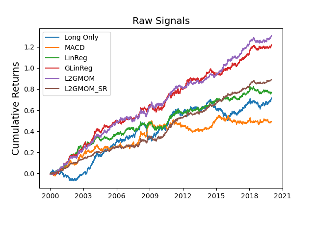
(a) Raw signals

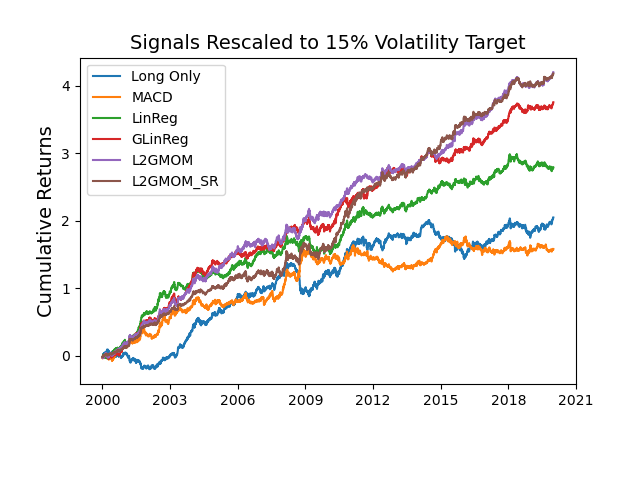
(b) Signals rescaled to 15% volatility target

Figure 1. The cumulative daily returns of the proposed strategy (L2GMOM/L2GMOM_SR) and four reference strategies (Long Only/MACD/LinReg/GLinReg) in different colours for the entire out-of-sample period from 2000 to 2020.

In evaluating the portfolio performance, we use the following annualised metrics in Table 1:

• Profitability: expected return and hit rate (the percentage of days with positive returns across the test period)

• Risk: daily volatility (vol.), downside deviation, maximum drawdown (MDD) and MDD duration (the percentage of days with MDD across the test period).

• Overall Performance: Sharpe ratio (expected return$/$vol.), Sortino ratio (expected return$/$downside deviation), Calmar ratio (expected return$/$MDD), and the average profits over the average loss $\left(\frac{\text{Avg. P}}{\text{Avg. L}}\right)$.

In order to have a better comparison between different strategies, we apply an additional layer of volatility scaling at the portfolio level to an annualised volatility target of 15% and report the above evaluation metrics. In Figure 1(a) and Figure 1(b), we plot the daily cumulative returns of raw signals and signals rescaled to 15% annual volatility of main strategies.

L2GMOM and GLinReg both outperform LinReg in terms of portfolio returns in both raw signals and signals rescaled to 15% target volatility. This suggests that considering the network effect in assets can greatly enhance profitability. L2GMOM also outperforming GLinReg indicates that optimising the graph with respect to portfolio performance can yield higher returns, which supports our conjecture that the separation of network construction in network momentum strategies may adversely affect the portfolio performance. In terms of portfolio risk, L2GMOM has a lower downside deviation and shorter MDD duration in both raw signals and signals rescaled to 15% target volatility, indicating that it manages risk more effectively. L2GMOM also outperforms GLinReg in terms of volatility, suggesting that optimising the graph with respect to portfolio performance can also reduce risk.

L2GMOM_SR has the lowest volatility, downside deviation, MDD, and MDD duration in the raw signal, indicating that optimising with the Sharpe ratio can significantly reduce risk. It is not surprising to observe a higher Sharpe ratio in L2GMOM_SR, which is consistent with the results in machine learning TSMOM (Lim et al., 2019). Note that, the returns of L2GMOM_SR drops in the raw signals, but the return is the highest in the volatility-scaled signals.

4.3. Diversification Analysis

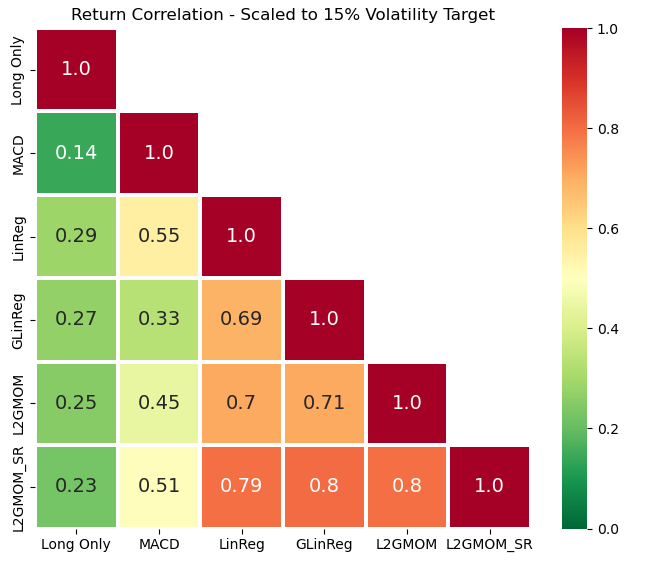
(a) Return Correlations

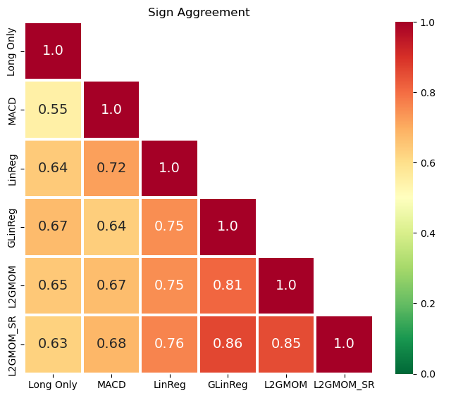
(b) Sign Agreement

Figure 2. A diversification analysis on the correlations and sign agreement of daily returns between the proposed strategies (L2GMOM/L2GMOM_SR) and four reference strategies (Long Only/MACD/LinReg/GLinReg) of the entire out-of-sample period from 2000 to 2020. The values of the pairwise correlation and sign agreement are marked in the corresponding square boxes.

To evaluate whether the signals constructed from the proposed models are different from the reference baselines, we calculated the correlation of daily returns between candidate signals in Figure 2(a). Besides, we calculate the percentage by how much the signals of two strategies have the same direction, also known as sign agreement in Figure 2(b). Note that LineReg, GLinReg, L2GMOM and L2GMOM_SR have the exactly same input momentum features.

From Figure 2(a) and Figure 2(b), we draw the following conclusions. The L2GMOM strategy, which incorporates graph learning and network momentum, shows moderate diversification potential with the model-free MACD strategy, as evidenced by their moderate return correlation and position sign agreement. Comparing L2GMOM with LinReg, which uses the same input but different momentum calculation methods, shows less diversification potential due to higher correlation and agreement. However, L2GMOM has better portfolio performance, showing it could be a better alternative strategy. Finally, L2GMOM, GLinReg, and L2GMOM_SR, all of which consider graph effects but differ in optimisation methods, show limited diversification potential due to high return correlations and sign agreements. Despite their different modelling approaches, the similar inputs and graph-based methods used by these strategies result in relatively high correlations, suggesting limited diversification benefits when combined in a portfolio.

4.4. Turnover Analysis

Following the convention of literature (Lim et al., 2019), we calculate the cost-adjusted Sharpe ratio from the adjusted returns:

(14) $$\tilde{r}_{i,t:t+1}^{\text{portfolio}}:=\frac{1}{N_{t}}\sum_{i=1}^{N_{t}}\Big{(}x_{i,t}\frac{\sigma_{\text{tgt}}}{\sigma_{i,t}}r_{i,t:t+1}-c\cdot\sigma_{i,t}\Big{|}\frac{x_{i,t}}{\sigma_{i,t}}-\frac{x_{i,t-1}}{\sigma_{i,t-1}}\Big{|}\Big{)}$$

where $c$ is the turnover cost in bps, varying from 0.5 to 5 bps. As ex-ante costs rise, all strategies see a drop in cost-adjusted Sharpe ratios. LinReg, a machine learning model, is most sensitive, turning negative at costs over 3 bps. GLinReg, which includes graph learning, fares better, maintaining a higher positive Sharpe ratios at 2 bps. The proposed models, L2GMOM and L2GMOM_SR, also stay positive at 3 bps, showing resilience to increasing costs. Thus, graph learning strategies like GLinReg, L2GMOM, and L2GMOM_SR offer better cost resilience than LinReg. The Long Only and MACD strategies, which are model-free, show a relatively gradual decrease in Sharpe ratio as ex-ante costs increase. To further reduce the turnover of machine learning strategies, (Lim et al., 2019) proposed including a turnover regularisation. This is an interesting avenue for future analysis.

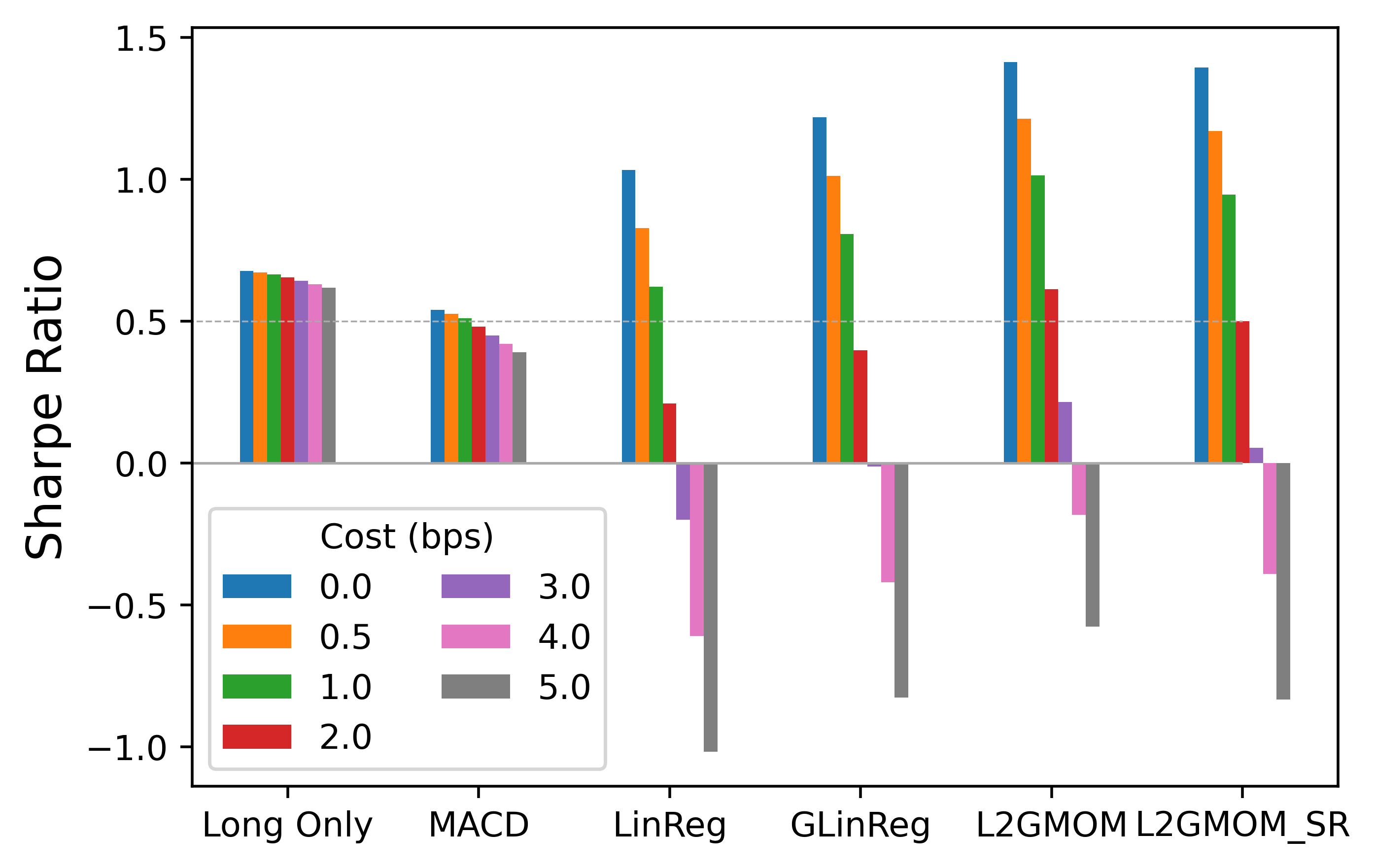
Figure 3. The cost-adjusted Sharpe ratio of the proposed strategies (L2GMOM/L2GMOM_SR) and four reference strategies (Long Only/MACD/LinReg/GLinReg) of the entire out-of-sample period from 2000 to 2020.

4.5. Network Analysis

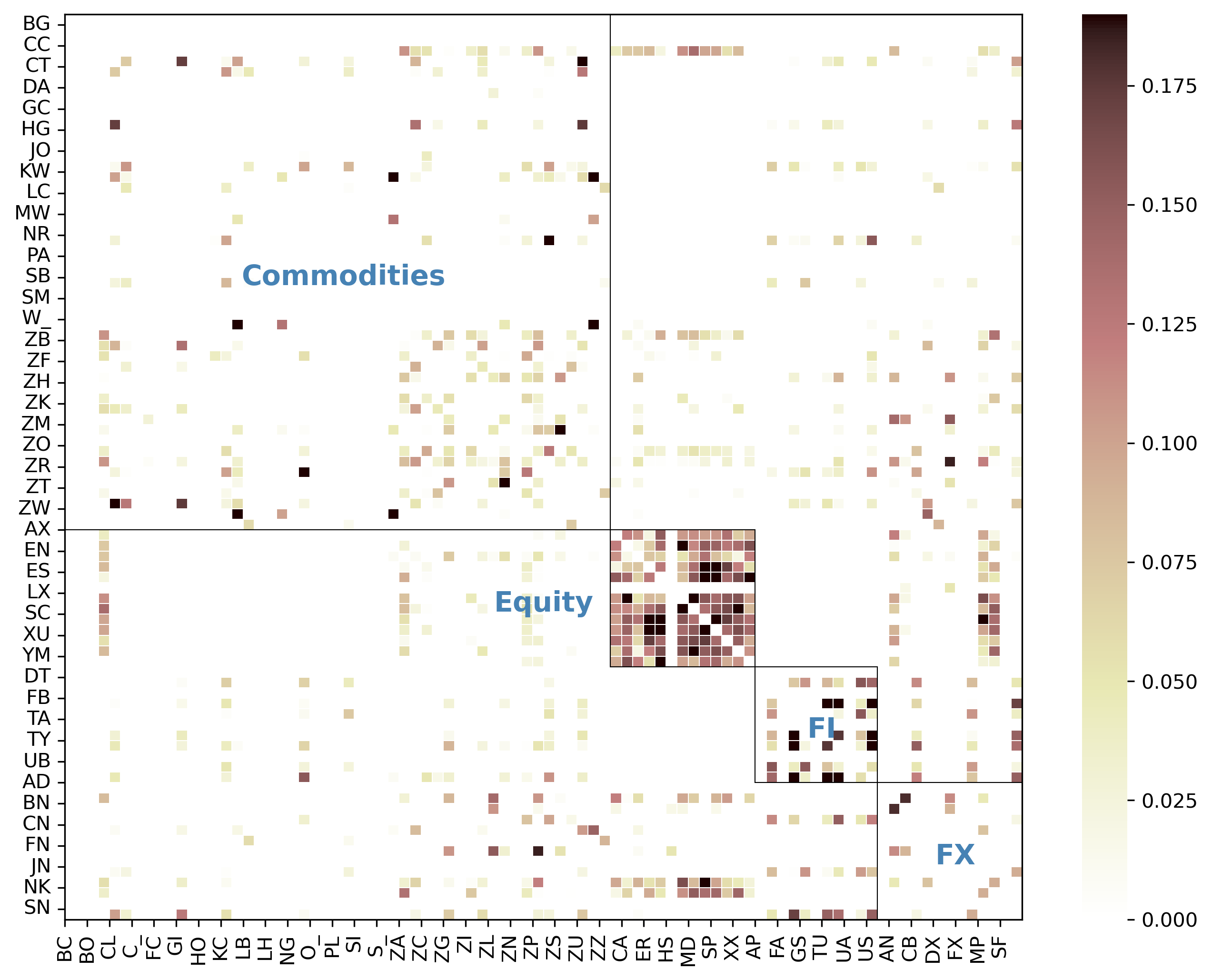
(a) 2008-01-03 from L2GMOM

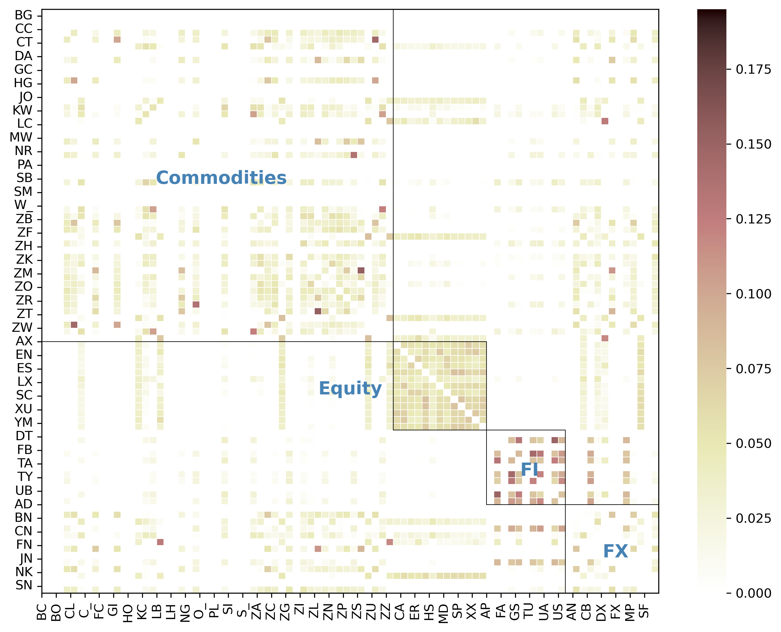
(b) 2008-01-03 from L2GMOM_SR

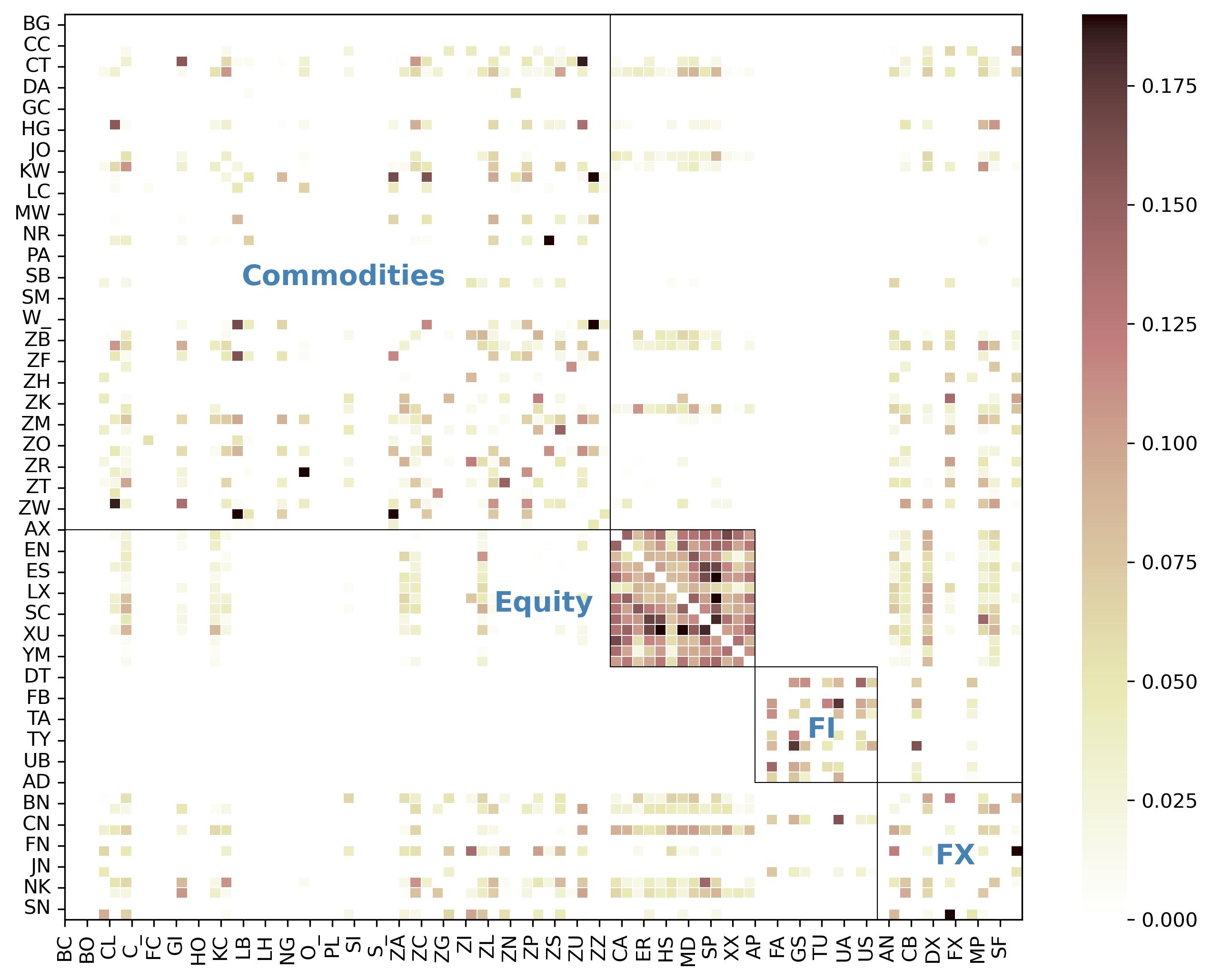
(c) 2010-01-04 from L2GMOM

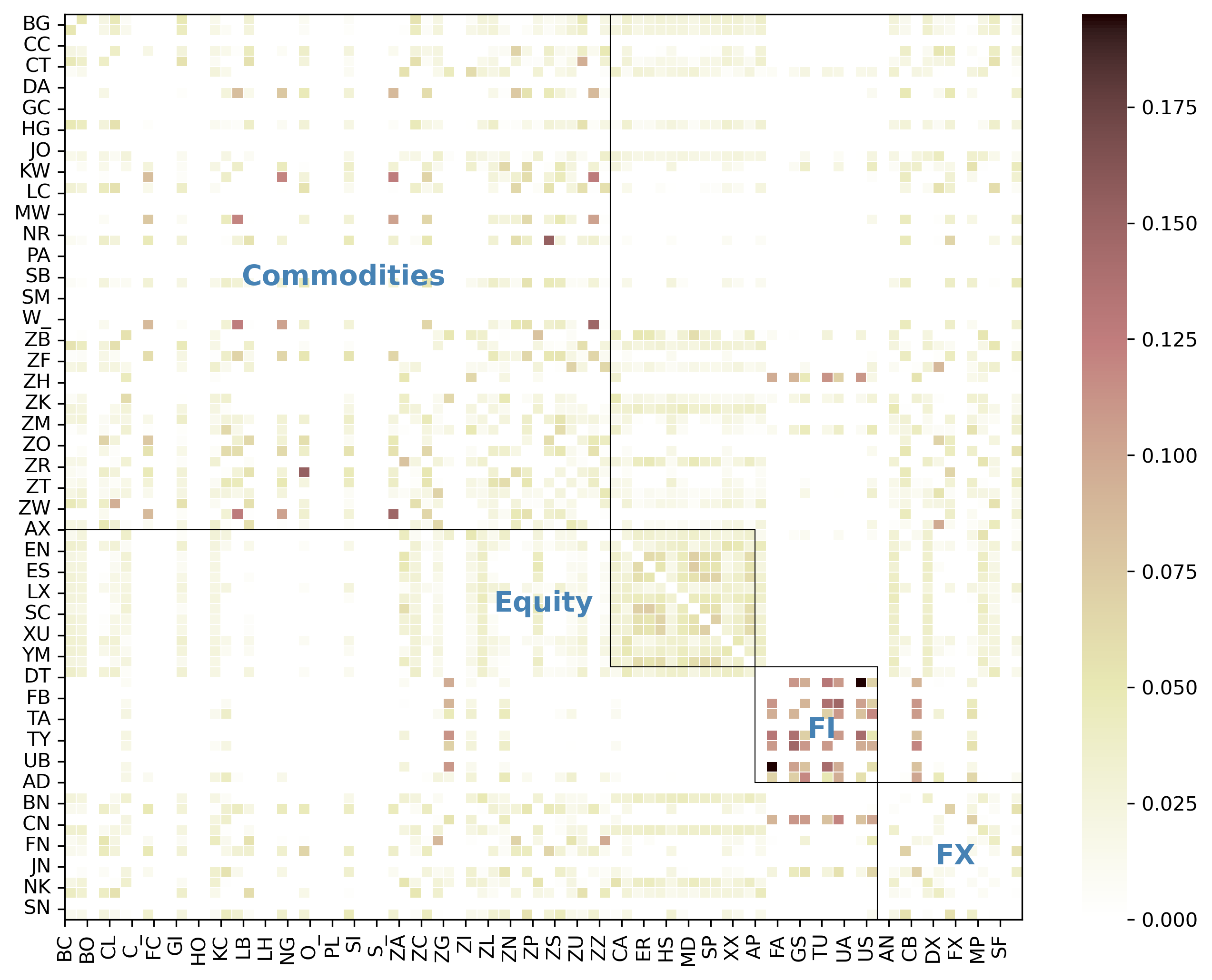
(d) 2010-01-04 from L2GMOM_SR

Figure 4. Momentum Spillover Analysis. Networks obtained from L2GMOM or L2GMOM_SR.

Figure 4 are example daily networks obtained from the proposed L2GMOM and L2GMOM_SR, specifically the output of Eq.(10b). We deliberately chose two different dates to exhibit, 2008-01-03 for the turbulent period and 2010-01-04 for the calm period. Note that there were some assets without any connections, because the input features for them were missing. The four subfigures demonstrate a strong community structure corresponding to four asset classes: commodities, equities, fixed income (FI), and foreign exchange (FX). The equities form a dense cluster, indicating a high degree of interconnection among equity assets. Inter-class connections are also observed, particularly between commodities and the other three asset classes. However, there is a notable absence of connections between equities and fixed income. This is reasonable given that these two asset classes often exhibit negative correlations and are used to hedge each other, suggesting no momentum spillover according to the strategy.

By comparing Figure 4(a) and 4(c), we can also capture some temporal variations in the momentum network structure. During calm periods (e.g. 2010-01-04), there are fewer inter-class connections between fixed income and the other assets. However, in turbulent times (e.g. Global Financial Crisis covering 2008-01-03), these connections increase, indicating a shift in momentum propagation under different market conditions.

The graphs obtained from the L2GMOM_SR strategy are denser with more similar edge weights, demonstrating the strategy’s tendency in reducing volatility. One possible explanation is that, by increasing the connections between assets, the strategy ensures that each asset receives momentum information passed from a broader range of assets, rather than relying on a few, thus enhancing the robustness and stability of the strategy.

5. Conclusion

In this paper, we present an innovative end-to-end graph machine learning framework for the construction of network momentum strategies, specifically two model variants: L2GMOM and L2GMOM_SR. Our framework effectively learns the graph adjacency matrix and optimises the momentum strategy directly from historical pricing data, reducing the dependence on costly linkage databases and financial expertise typically needed for constructing network momentum factors, such as those derived from supply chain data.

Our models exceed the performance of traditional time series momentum strategies in both portfolio returns and risk management across 64 continuous futures contracts. Moreover, our models are highly interpretable, providing explicit networks as a byproduct. These networks not only represent the similarity between the momentum features of these assets, but are also optimised with respect to portfolio performance. This offers a powerful interpretation of the interconnections that can aid in constructing network momentum strategies. By analysing these learned networks, we uncover the community structure and temporal variations that align with common financial sense.

Appendix A Dataset Details

Table 2. The Pinnacle Universe

Ticker	Description	Period	Ticker	Description	Period
Commodities:			Equities:
BC	BRENT CRUDE OIL, composite	2010-2020	AX	GERMAN DAX INDEX	1999-2020
BG	BRENT GASOIL, composite	2010-2020	CA	CAC40 INDEX	2000-2020
CC	COCOA	1990-2020	EN	NASDAQ, MINI	2001-2020
CL	CRUDE OIL	1990-2020	ER	RUSSELL 2000, MINI	2004-2020
CT	COTTON #2	1990-2020	ES	S&P 500, MINI	1999-2020
DA	MILK III, composite	1999-2020	HS	HANG SENG INDEX	1999-2020
GI	GOLDMAN SAKS C. I.	1995-2020	LX	FTSE 100 INDEX	1991-2020
JO	ORANGE JUICE	1990-2020	MD	S&P 400, MINI, electronic	1994-2020
KC	COFFEE	1990-2020	SC	S&P 500, composite	1996-2020
KW	WHEAT	1990-2020	SP	S&P 500, day session	1990-2020
LB	LUMBER	1990-2020	XU	DOW JONES EUROSTOXX 50	2003-2020
MW	WHEAT, MINN	1990-2020	XX	DOW JONES STOXX 50	2004-2020
NR	NATURAL GAS	1990-2020	YM	DOW JONES, MINI ($5.00)	2004-2020
SB	SUGAR #11	1990-2020	Fixed Income:
W_	WHEAT, CBOT	1990-2018	AP	AUSTRALIAN PRICE INDEX	2010-2020
ZA	PALLADIUM, electronic	1990-2020	DT	EURO BOND (BUND)	1991-2020
ZB	RBOB, electronic	1990-2020	FB	T-NOTE, 5yr composite	1990-2020
ZC	CORN, electronic	1990-2020	GS	GILT, LONG BOND	1991-2020
ZF	FEEDER CATTLE, electronic	1990-2020	TU	T-NOTES, 2yr composite	1992-2020
ZG	GOLD, electronic	1990-2020	TY	T-NOTE, 10yr composite	1990-2020
ZI	SILVER, electronic	1990-2020	UB	EURO BOBL	2000-2020
ZK	COPPER, electronic	1990-2020	US	T-BONDS, composite	1990-2020
ZL	SOYBEAN OIL, electronic	1990-2020	Currencies:
ZM	SOYBEAN MEAL, electronic	1990-2020	AN	AUSTRALIAN $$, day session	1990-2020
ZN	NATURAL GAS, electronic	1992-2020	BN	BRITISH POUND, composite	1990-2020
ZO	OATS, electronic	1990-2020	CB	CANADIAN 10YR BOND	1996-2020
ZP	PLATINUM, electronic	1990-2020	CN	CANADIAN $$, composite	1990-2020
ZR	ROUGH RICE, electronic	1990-2020	DX	US DOLLAR INDEX	1990-2020
ZS	SOYBEANS electronic	1990-2020	FN	EURO, composite	1990-2020
ZT	LIVE CATTLE, electronic	1990-2020	JN	JAPANESE YEN, composite	1990-2020
ZU	CRUDE OIL, electronic	1990-2020	MP	MEXICAN PESO	1997-2020
ZW	WHEAT electronic	1990-2020	NK	NIKKEI INDEX	1992-2020
ZZ	LEAN HOGS, electronic	1990-2020	SN	SWISS FRANC, composite	1990-2020

The backtest was primarily conducted with the Pinnacle Data Corp CLC Database. We have access to a robust dataset comprising 98 ratio-adjusted continuous futures contracts dating back to 1990. However, for the purpose of this study, we narrowed our focus to a subset of 64 assets, as listed in Table 2.

References

- (1)
- Ali and Hirshleifer (2020) Usman Ali and David Hirshleifer. 2020. Shared Analyst Coverage: Unifying Momentum Spillover Effects. Journal of Financial Economics 136, 3 (June 2020), 649–675.
- Baz et al. (2015) Jamil Baz, Nicolas Granger, Campbell R. Harvey, Nicolas Le Roux, and Sandy Rattray. 2015. Dissecting Investment Strategies in the Cross Section and Time Series. (Dec. 2015).
- Boni and Womack (2006) Leslie Boni and Kent L. Womack. 2006. Analysts, Industries, and Price Momentum. Journal of Financial and Quantitative Analysis 41, 1 (March 2006), 85–109.
- Cohen and Frazzini (2008) Lauren Cohen and Andrea Frazzini. 2008. Economic Links and Predictable Returns. The Journal of Finance 63, 4 (2008), 1977–2011.
- Dong et al. (2016) Xiaowen Dong, Dorina Thanou, Pascal Frossard, and Pierre Vandergheynst. 2016. Learning Laplacian Matrix in Smooth Graph Signal Representations. IEEE Transactions on Signal Processing 64, 23 (2016), 6160–6173.
- Dong et al. (2019) Xiaowen Dong, Dorina Thanou, Michael Rabbat, and Pascal Frossard. 2019. Learning Graphs from Data: A Signal Representation Perspective. IEEE Signal Processing Magazine 36, 3 (May 2019), 44–63.
- Kalofolias (2016) Vassilis Kalofolias. 2016. How to Learn a Graph from Smooth Signals. Proceedings of the 19th International Conference on Artificial Intelligence and Statistics (May 2016), 920–929.
- Korniotis and Kumar (2013) George M. Korniotis and Alok Kumar. 2013. State-Level Business Cycles and Local Return Predictability. The Journal of Finance 68, 3 (2013), 1037–1096.
- Lee et al. (2019) Charles M.C. Lee, Stephen Teng Sun, Rongfei Wang, and Ran Zhang. 2019. Technological Links and Predictable Returns. Journal of Financial Economics 132, 3 (June 2019), 76–96.
- Lim et al. (2019) Bryan Lim, Stefan Zohren, and Stephen Roberts. 2019. Enhancing Time Series Momentum Strategies Using Deep Neural Networks. The Journal of Financial Data Science 1, 4 (2019), 19–38.
- Liu et al. (2023) Tom Liu, Stephen Roberts, and Stefan Zohren. 2023. Deep Inception Networks: A General End-to-End Framework for Multi-asset Quantitative Strategies. arXiv:2307.05522 [q-fin]
- Mateos et al. (2019) Gonzalo Mateos, Santiago Segarra, Antonio G. Marques, and Alejandro Ribeiro. 2019. Connecting the Dots: Identifying Network Structure via Graph Signal Processing. IEEE Signal Processing Magazine 36, 3 (May 2019), 16–43.
- Menzly and Ozbas (2010) Lior Menzly and Oguzhan Ozbas. 2010. Market Segmentation and Cross-predictability of Returns. The Journal of Finance 65, 4 (2010), 1555–1580.
- Moskowitz and Grinblatt (1999) Tobias J. Moskowitz and Mark Grinblatt. 1999. Do Industries Explain Momentum? The Journal of Finance 54, 4 (Aug. 1999), 1249–1290.
- Moskowitz et al. (2012) Tobias J. Moskowitz, Yao Hua Ooi, and Lasse Heje Pedersen. 2012. Time Series Momentum. Journal of Financial Economics 104, 2 (May 2012), 228–250.
- Parsons et al. (2020) Christopher A Parsons, Riccardo Sabbatucci, and Sheridan Titman. 2020. Geographic Lead-Lag Effects. The Review of Financial Studies 33, 10 (Oct. 2020), 4721–4770.
- Pu et al. (2021) Xingyue Pu, Tianyue Cao, Xiaoyun Zhang, Xiaowen Dong, and Siheng Chen. 2021. Learning to Learn Graph Topologies. Advances in Neural Information Processing Systems 34 (2021), 4249–4262.
- Tan et al. (2023) Wee Ling Tan, Stephen Roberts, and Stefan Zohren. 2023. Spatio-Temporal Momentum: Jointly Learning Time-Series and Cross-Sectional Strategies. arXiv:2302.10175 [cs, q-fin, stat]
- Wan et al. (2021) Xingchen Wan, Jie Yang, Slavi Marinov, Jan-Peter Calliess, Stefan Zohren, and Xiaowen Dong. 2021. Sentiment Correlation in Financial News Networks and Associated Market Movements. Scientific Reports 11, 1 (Feb. 2021), 3062.
- Wood et al. (2022) Kieran Wood, Sven Giegerich, Stephen Roberts, and Stefan Zohren. 2022. Trading with the Momentum Transformer: An Intelligent and Interpretable Architecture. arXiv:2112.08534 [cs, q-fin, stat]
- Yamamoto et al. (2021) Rei Yamamoto, Naoya Kawadai, and Hiroki Miyahara. 2021. Momentum Information Propagation through Global Supply Chain Networks. The Journal of Portfolio Management 47, 8 (July 2021), 197–211.