Uldp-FL: Federated Learning with Across-Silo User-Level Differential Privacy

Abstract.

Differentially Private Federated Learning (DP-FL) has garnered attention as a collaborative machine learning approach that ensures formal privacy. Most DP-FL approaches ensure DP at the record-level within each silo for cross-silo FL. However, a single user’s data may extend across multiple silos, and the desired user-level DP guarantee for such a setting remains unknown. In this study, we present Uldp-FL, a novel FL framework designed to guarantee user-level DP in cross-silo FL where a single user’s data may belong to multiple silos. Our proposed algorithm directly ensures user-level DP through per-user weighted clipping, departing from group-privacy approaches. We provide a theoretical analysis of the algorithm’s privacy and utility. Additionally, we enhance the utility of the proposed algorithm with an enhanced weighting strategy based on user record distribution and design a novel private protocol that ensures no additional information is revealed to the silos and the server. Experiments on real-world datasets show substantial improvements in our methods in privacy-utility trade-offs under user-level DP compared to baseline methods. To the best of our knowledge, our work is the first FL framework that effectively provides user-level DP in the general cross-silo FL setting.

PVLDB Reference Format:
PVLDB, (): , .
doi:

PVLDB Artifact Availability:
The source code, data, and/or other artifacts have been made available at %leave␣empty␣if␣no␣availability␣url␣should␣be␣sethttps://github.com/FumiyukiKato/uldp-fl.

1. Introduction

Federated Learning (FL) (McMahan et al., 2016) is a collaborative machine learning (ML) scheme in which multiple parties train a single global model without sharing training data. FL has attracted industry attention (Paulik et al., 2021; Ramaswamy et al., 2019) as concerns about the privacy of training data have become more serious, as exemplified by GDPR (Goddard, 2017). It should be noted that FL itself does not provide rigorous privacy protection for the trained model (Nasr et al., 2019; Zhao et al., 2020). Differentially Private FL (DP-FL) (Geyer et al., 2017; Kairouz et al., 2021) further guarantees a formal privacy for trained models based on differential privacy (DP) (Dwork, 2006).

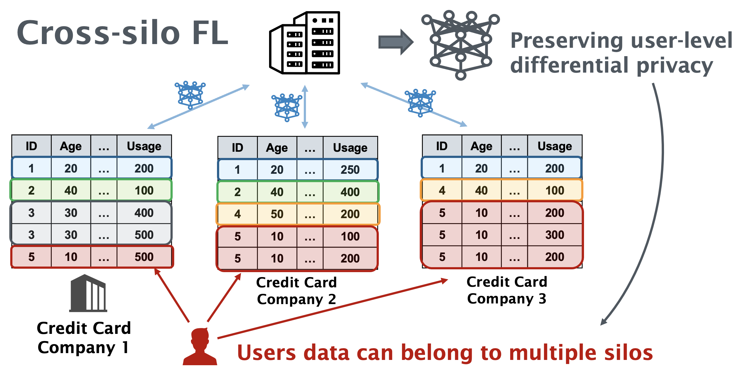
Figure 1. In cross-silo FL, records belonging to the same user can exist across silos, e.g., a user can use several credit card companies. In this study, we investigate how to train models satisfying user-level DP in this setting.

Although DP is the de facto standard in the field of statistical privacy protection, it has a theoretical limitation. The standard DP definition takes a single record as a unit of privacy. This can easily break down in realistic settings where one user may provide multiple records, potentially deteriorating the privacy loss bound of DP. To address this, the notion of user-level DP has been studied (Liu et al., 2020; Levy et al., 2021; Wilson et al., 2020; Amin et al., 2019). In user-level DP, all records belonging to a single user are considered as a unit of privacy, which is a stricter definition than standard DP. We distinguish user-level DP from group-privacy (Dwork et al., 2014), which considers any $k$ records as privacy units. User-level DP has also been studied in the FL context (Erlingsson et al., 2020; Geyer et al., 2017; McMahan et al., 2018, 2017; Kairouz et al., 2021). However, these studies focus on the cross-device FL setting, where one user’s data belongs to a single device only.

Cross-silo FL (Ogier du Terrail et al., 2022; Liu et al., 2022; Lowy and Razaviyayn, 2023; Lowy et al., 2023) is a practical variant of FL in which a relatively small number of silos (e.g., hospitals or credit card companies) participate in training rounds. In cross-silo FL, unlike in cross-device FL, a single user can have multiple records across silos, as shown in Figure 1. Existing cross-silo DP-FL studies (Liu et al., 2022; Lowy and Razaviyayn, 2023; Lowy et al., 2023) have focused on record-level DP for each silo; user-level DP across silos has not been studied. Therefore, an important research question arises: How do we design an FL framework that guarantees user-level DP across silos in cross-silo FL?

A baseline solution for guaranteeing user-level DP is to bound user contributions (number of records per user) as in (Wilson et al., 2020; Amin et al., 2019) and then utilize group-privacy property of DP (Dwork et al., 2014). Group-privacy simply extends the indistinguishability of the record-level DP to multiple records. We can convert any DP algorithm to group-privacy version of DP (see Lemma 8, 9 later), which we formally define as Group DP (GDP). However, this approach can be impractical due to the super-linear privacy bound degradation of conversion to GDP and the need to appropriately limit the maximum number of user records (group size) in a distributed environment. In particular, the former issue is a fundamental limitation for DP and highlights the need to develop algorithms that directly satisfy user-level DP without requiring conversion to GDP.

In this study, we present Uldp-FL, a novel cross-silo FL framework, designed to directly ensure user-level DP through per-user weighted clipping and an effective weighting strategy. Additionally, we propose a novel private weighted aggregation protocol for implementing the weighting algorithm. This protocol ensures the private information of each silo is protected from both the server and other silos. The limitation of previous methods that relied solely on the Paillier cryptosystem for private weighted summation (Alexandru and Pappas, 2022) is that the raw data is visible to the party with the secret key. We overcome this limitation by using a combination of several cryptographic techniques such as Paillier, Secure Aggregation (Bonawitz et al., 2017), and Multiplicative blinding (Damgård et al., 2007). To the best of our knowledge, our work is the first FL framework that effectively provides user-level DP across silos in the general cross-silo FL setting (as in Figure 1).

The contributions of this work are summarized as follows:

• We propose the Uldp-FL framework and design baseline algorithms capable of achieving user-level DP across silos. The baseline algorithms limit the maximum number of records per user and use group-privacy property of DP.

• We then propose ULDP-AVG/SGD algorithms that directly satisfy user-level DP by implementing user-level weighted clipping within each silo, effectively bounding user-level sensitivity even when a single user may have unbounded number of records across silos. We provide theoretical analysis, including privacy bound and convergence analysis.

• We evaluate our proposed method and baseline approaches through comprehensive experiments on various real-world datasets. The results underscore that our proposed method yields superior trade-offs between privacy and utility compared to the baseline approaches.

• We further design an effective method by refining the weighting strategy for individual user-level clipping bounds. Since this approach may lead to additional privacy leaks, we develop a novel private weighted aggregation protocol employing several cryptographic techniques. We evaluate the extra computational overhead of the proposed private protocol using real-world benchmark scenarios.

2. Background & Preliminaries

2.1. Cross-silo Federated learning

In this work, we consider the following cross-silo FL scenario. We have a central aggregation server and a set of silos $S$ participating in all rounds. In each round, the server aggregates models from all silos and then redistributes the aggregated models. Each silo $s\in S$ optimizes a local model $f_{s}$, which is the expectation of a loss function $F(x;\xi)$ that may be non-convex, where $x\in\mathbb{R}^{d}$ denotes the model parameters and $\xi$ denotes the data sample, and the expectation is taken over local data distribution $\mathcal{D}_{s}$. In cross-silo FL, we optimize this global model parameter cooperatively across all silos. Formally, the overarching goal in FL can be formulated as follows:

(1) $$\min_{x}\,\left\{f(x):=\frac{1}{|S|}\sum_{s\in S}{f_{s}(x)}\right\},\,f_{s}(x):=\mathbb{E}_{\xi\sim\mathcal{D}_{s}}F(x;\xi).$$

Additionally, in our work, we have user set $U$ across all datasets across silos, where each record belongs to one user $u\in U$, and each user may have multiple records in one silo and across multiple silos. Each silo $s$ has local objectives for each user $u$, $f_{s,u}:=\mathbb{E}_{\xi\sim\mathcal{D}_{s,u}}F(x;\xi)$, where $\mathcal{D}_{s,u}$ is the data distribution of $s$ and $u$. In round $t\in[T]$ in FL, the global model parameter is denoted as $x_{t}$.

Note that this modeling is clearly different from cross-device FL in that there is no constraint that one user should belong to one device. Records from one user can belong to multiple silos. For example, the same customer may use several credit card companies, etc. Additionally, all silos participate in all training rounds, unlike the probabilistic participation in cross-device FL (McMahan et al., 2017), and the number of silos $|S|$ is small, around 2 to 100.

2.2. Differential Privacy

Differential privacy. DP (Dwork, 2006) is a rigorous mathematical privacy definition that quantitatively evaluates the degree of privacy protection for outputs.

Definition 0 ($(\epsilon,\delta)$-DP).

A randomized mechanism $\mathcal{M}:\mathcal{D}\rightarrow\mathcal{Z}$ satisfies $(\epsilon,\delta)$-DP if, for any two input databases $D,D^{\prime}\in\mathcal{D}$ s.t. $D^{\prime}$ differs from $D$ in at most one record and any subset of outputs $Z\subseteq\mathcal{Z}$, it holds that

(2) $$\Pr[\mathcal{M}(D)\in Z]\leq\exp(\epsilon)\Pr[\mathcal{M}(D^{\prime})\in Z]+\delta.$$

We call databases $D$ and $D^{\prime}$ as neighboring databases. The maximum difference of the output for any neighboring database is referred to as sensitivity. We label the original definition as record-level DP because the neighboring databases differ in only one record.

Rényi differential privacy. Rényi DP (RDP) (Mironov, 2017) is a variant of approximate DP based on Rényi divergence. RDP is preferable because it is easy to use for Gaussian mechanism (Mironov, 2017) and has a tighter bound than the standard composition theorems. The following lemmas give the bounds of the RDP for a typical mechanism and are used to further convert it to an original DP bound.

Definition 0 ($(\alpha,\rho)$-RDP (Mironov, 2017)).

Given a real number $\alpha\in(1,\infty)$ and privacy parameter $\rho\geq 0$, a randomized mechanism $\mathcal{M}$ satisfies $(\alpha,\rho)$-RDP if for any two neighboring datasets $D,D^{\prime}\in\mathcal{D}$ s.t. $D^{\prime}$ differs from $D$ in at most one record, we have that $D_{\alpha}(\mathcal{M}(D)||\mathcal{M}(D^{\prime}))\leq\rho$ where $D_{\alpha}(\mathcal{M}(D)||\mathcal{M}(D^{\prime}))$ is the Rényi divergence between $\mathcal{M}(D)$ and $\mathcal{M}(D^{\prime})$ and is given by

$$D_{\alpha}(\mathcal{M}(D)||\mathcal{M}(D^{\prime})):=\frac{1}{\alpha-1}\log{\mathbb{E}\left[\left(\frac{\mathcal{M}(D)}{\mathcal{M}(D^{\prime})}\right)^{\alpha}\right]}\leq\rho,$$

where the expectation is taken over the output of $\mathcal{M}(D)$.

Lemma 0 (RDP composition (Mironov, 2017)).

If $\mathcal{M}_{1}$ satisfies $(\alpha,\rho_{1})$-RDP and $\mathcal{M}_{2}$ satisfies $(\alpha,\rho_{2})$, then their composition $\mathcal{M}_{1}\circ\mathcal{M}_{2}$ satisfies $(\alpha,\rho_{1}+\rho_{2})$-RDP.

Lemma 0 (RDP to DP conversion (Balle et al., 2020)).

If $\mathcal{M}$ satisfies $(\alpha,\rho)$-RDP, then it also satisfies $(\rho^{\prime},\delta)$-DP for any $0<\delta<1$ such that

$$\rho^{\prime}=\rho+\log{\frac{\alpha-1}{\alpha}}-\frac{\log{\delta}+\log{\alpha}}{\alpha-1}.$$

Lemma 0 (RDP Gaussian mechanism (Mironov, 2017)).

If $f:D\rightarrow\mathbb{R}^{d}$ has $\ell 2$-sensitivity $\Delta_{f}$, then the Gaussian mechanism $G_{f}(\cdot):=f(\cdot)+\mathcal{N}(0,I\sigma^{2}\Delta_{f}^{2})$ is $(\alpha,\alpha/2\sigma^{2})$-RDP for any $\alpha>1$.

Lemma 0 (RDP for sub-sampled Gaussian mechanism (Wang et al., 2019)).

Let $\alpha\in\mathbb{N}$ with $\alpha\geq 2$ and $0<q<1$ be a ratio of sub-sampling operation $Samp_{q}$. Let $G^{\prime}_{f}(\cdot):=G_{f}\circ Samp_{q}(\cdot)$ be a sub-sampled Gaussian mechanism. Then, $G^{\prime}_{f}$ is $(\alpha,\rho^{\prime}(\alpha,\sigma))$-RDP where

$$\rho^{\prime}(\alpha,\sigma)\leq\frac{1}{\alpha-1}\log\biggl{(}1+2q^{2}\binom{\alpha}{2} \min{\{2(e^{1/\sigma^{2}}-1),e^{1/\sigma^{2}}\}}$$

$$+\sum_{j=3}^{\alpha}{2q^{j}\binom{\alpha}{j}e^{j(j-1)/2\sigma^{2}}}\biggl{)}.$$

In general, we can compute tighter numerical bounds along with the closed-form upper bounds described above (Wang et al., 2019; Mironov et al., 2019).

Group differential privacy. To extend privacy guarantees to multiple records, group-privacy (Dwork et al., 2014) has been explored as a solution. We refer to the group-privacy version of DP as Group DP (GDP).

Definition 0 ($(k,\epsilon,\delta)$-GDP).

A randomized mechanism $\mathcal{M}:\mathcal{D}\rightarrow\mathcal{Z}$ satisfies $(k,\epsilon,\delta)$-GDP if, for any two input databases $D,D^{\prime}\in\mathcal{D}$, s.t. $D^{\prime}$ differs from $D$ in at most $k$ records and any subset of outputs $Z\subseteq\mathcal{Z}$, Eq. (2) holds.

GDP is a versatile privacy definition, as it can be applied to existing DP mechanisms without modification.

To convert DP to GDP, it is known that any $(\epsilon,0)$-DP mechanism satisfies $(k,k\epsilon,0)$-GDP (Dwork et al., 2014). However, in the case of any $\delta>0$, $\delta$ increases super-linearly (Kamath, 2020), leading to a much larger $\epsilon$.

Lemma 0 (Group privacy conversion (record-level DP to GDP) (Kamath, 2020)).

If $f$ is $(\epsilon,\delta)$-DP, for any two input databases $D,D^{\prime}\in\mathcal{D}$ s.t. $D^{\prime}$ differs from $D$ in at most $k$ records and any subset of outputs $Z\subseteq\mathcal{Z}$, it holds that

$$\Pr[f(D)\in Z]\leq\exp(k\epsilon)\Pr[f(D^{\prime})\in Z]+ke^{(k-1)\epsilon}\delta.$$

It means when $f$ is $(\epsilon,\delta)$-DP, $f$ satisfies $(k,k\epsilon,k\exp^{(k-1)\epsilon}\delta)$-GDP.

Also, we can compute GDP using group-privacy property of Rényi DP (Mironov, 2017). First, we calculate the RDP of the algorithm, then convert it to group version of RDP, and subsequently to GDP.

Lemma 0 (Group-privacy of RDP (record-level DP to GDP) (Mironov, 2017)).

If $f:D\rightarrow\mathbb{R}^{d}$ is $(\alpha,\rho)$-RDP, $g:D^{\prime}\rightarrow D$ is $k$-stable and $\alpha\geq 2^{k+1}$, then $f\circ g$ is $(\alpha/2^{k},3^{k}\rho)$-RDP.

Here, group-privacy property is defined using a notion of $k$-stable transformation (McSherry, 2009). $g:D^{\prime}\rightarrow D$ is $k$-stable if $g(A)$ and $g(B)$ are neighboring in $D$ implies that there exists a sequence of length $c+1$ so that $D_{0}=A,...,D_{c}=B$ and all $(D_{i},D_{i+1})$ are neighboring in $D^{\prime}$. This privacy notion corresponds to $(k,\cdot,\cdot)$-GDP in Definition 7.

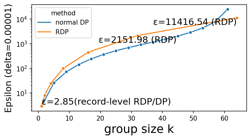
Figure 2. Group-privacy conversion results.

Here, to highlight the significant privacy degradation of GDP, we conduct a pre-experiment and show the converted privacy bounds for increasing group sizes. Figure 2 illustrates a numerical comparison of the group-privacy conversion from DP to GDP with normal DP (Lemma 8) and RDP (Lemma 9). To compute the final GDP privacy bounds, we repeatedly run the Gaussian mechanism with $\sigma=5.0$ and a sampling rate of $0.01$ for $10^{5}$ iterations, emulating a typical DP-SGD (Abadi et al., 2016) (which is the common mechanism for DP ML) setup. We use a fixed $\delta=10^{-5}$ and vary the group size $k=1,2,4,8,16,32,64$. To compute GDP, RDP for sub-sampled Gaussian mechanisms is calculated according to (Wang et al., 2019). We then compute GDP using group-privacy of RDP by Lemma 9. For normal DP, the computed RDP is converted to normal DP by Lemma 4, and then to GDP by Lemma 8.

When converting from normal DP to GDP, computing the final $\epsilon$ at a fixed $\delta$ is challenging. In Lemma 4, the output $\epsilon$ (denoted as $\epsilon_{l\ref{lemma:rdp_conversion}}$) depends on the input $\delta$ (denoted as $\delta_{l\ref{lemma:rdp_conversion}}$), and the final $\delta$ (denoted as $\delta_{l\ref{lemma:normaldp_group_privacy}}$) output by Lemma 8 depends on both $\epsilon_{l\ref{lemma:rdp_conversion}}$ and $\delta_{l\ref{lemma:rdp_conversion}}$. Therefore, we repeatedly select $\delta_{l\ref{lemma:rdp_conversion}}$ in a binary search manner, compute $\epsilon_{l\ref{lemma:rdp_conversion}}$ and $\delta_{l\ref{lemma:rdp_conversion}}$, and finally report the $\epsilon$ when the difference between $\delta_{l\ref{lemma:rdp_conversion}}$ and $\delta=10^{-5}$ is sufficiently small (accuracy by $10^{-8}$) as the $\epsilon$ of GDP. Note that this method does not guarantee achieving the optimal $\epsilon$ for the given $\delta$, but it finds a reasonable $\epsilon$.

In the figure, we plot various group sizes, $k$, on the x-axis and $\epsilon$ of GDP at a fixed $\delta=10^{-5}$ on the y-axis. Significantly, the results indicate that as the group size $k$ increases, $\epsilon$ grows rapidly, highlighting a considerable degradation in the privacy bound of GDP. For instance, with $\epsilon=2.85$ at record-level ($k=1$), the value reaches 2100 for only $k=32$, and 11400 at $k=64$. While there might be some looseness in the group-privacy conversion of RDP compared to normal DP for some small group sizes, the difference is relatively minor (roughly three times at most). The drastic change in normal DP with large group size is due to the numerical instability in our conversion procedure. RDP’s conversion is easier to compute with a fixed $\delta$. Hence, we utilize RDP’s conversion in the experiments.

2.3. Differentially Private FL

DP has been applied to the FL paradigm, with the goal of ensuring that the trained model satisfies DP. A popular DP variant in the context of cross-device FL is user-level DP (also known as client-level DP) (Geyer et al., 2017; Agarwal et al., 2021; Kairouz et al., 2021). Informally, this definition ensures indistinguishability for device participation and has demonstrated a favorable privacy-utility trade-off if the number of clients are sufficient, even with large-scale models (McMahan et al., 2017). These studies often employ secure aggregation (Bonawitz et al., 2017; Bell et al., 2020) to mitigate the need for trust in other parties during FL model training. This is achieved by allowing the server and other silos to only access appropriately perturbed models after aggregation, often referred to as Distributed DP (Kairouz et al., 2021; Cheu et al., 2019). In particular, shuffling-based variants have recently gained attention (Cheu et al., 2019; Liew et al., 2022; Takagi et al., 2023) and are being deployed in FL (Girgis et al., 2021), which also provides user-level DP. All of these studies assume that a single device holds all records for a single user, i.e., cross-device FL. However, in a cross-silo setting, this definition does not extend meaningful privacy protection to individual users when they possess multiple records across silos.

Another DP definition in cross-silo FL offers record-level DP within each silo (Liu et al., 2022; Lowy and Razaviyayn, 2023; Lowy et al., 2023), referred to as Silo-specific sample-level or Inter-silo record-level DP. These studies suggest that record-level DP can guarantee user-level DP through group-privacy. However, they cannot account for settings where a single user can have records across multiple silos. As far as we know, no method exists for training models that satisfy user-level DP in cross-silo FL where a single user’s records can extend across multiple silos.

3. Uldp-FL Framework

3.1. Trust model and Assumptions

We assume that all (two or more) silos and aggregation servers are semi-honest (or honest-but-curious). This is a typical assumption in prior works (Bonawitz et al., 2017; So et al., 2023). In our study, aggregation is performed using secure aggregation to ensure that the server only gains access to the model after aggregation (Kairouz et al., 2021). All communications between the server and silos are encrypted with SSL/TLS, and third parties with the ability to snoop on communications cannot access any information except for the final trained model. We assume that there is no collusion, which is reasonable given that silos are socially separate institutions (such as different hospitals or companies). Additionally, in our scenario, we assume that record linkage (Vatsalan et al., 2017) across silos has already been completed, resulting in shared common user IDs. Both the server and the silos are aware of the total number of users $|U|$ and the number of silos $|S|$. When user (device)-level sub-sampling is employed for DP amplification, only the server is permitted to know the sub-sampling results for each round (Kairouz et al., 2021; Agarwal et al., 2021). Note that all these assumptions do not affect the privacy guarantees of the final model released to external users.

3.2. Privacy definition

In contrast to GDP, which offers indistinguishability for any $k$ records, user-level DP (Levy et al., 2021; Geyer et al., 2017) provides a more reasonable user-level indistinguishability regardless of the number of the records. While (Geyer et al., 2017) focuses solely on a cross-device FL context, we re-establish user-level DP (ULDP) in the cross-silo setting as follows:

Definition 0 ($(\epsilon,\delta)$-User-Level DP (ULDP)).

A randomized mechanism $\mathcal{M}:\mathcal{D}\rightarrow\mathcal{Z}$ satisfies $(\epsilon,\delta)$-ULDP if, for any two input databases across silos $D,D^{\prime}\in\mathcal{D}$, s.t. $D^{\prime}$ differs from $D$ in at most one user’s records, and any $Z\subseteq\mathcal{Z}$, Eq. (2) holds.

The fundamental difference of user-level DP from record-level DP lies in the definition of the neighboring databases. The user-level neighboring database inherently defines user-level sensitivity. Additionally, it is important to emphasize that the input database $D$ represents the comprehensive database spanning across silos.

If the number of records per user in the database is less than or equal to $k$, it is clear that GDP is a generalization of ULDP, and the following proposition holds.

Proposition 0.

If a randomized mechanism $\mathcal{M}$ is $(k,\epsilon,\delta)$-GDP with input database $D$ in which any user has at most $k$ records, the mechanism $\mathcal{M}$ with input database $D$ also satisfies $(\epsilon,\delta)$-ULDP.

One drawback of GDP is the challenge of determining the appropriate value for $k$. Setting $k$ to the maximum number of records associated with any individual user could lead to introducing excessive noise to achieve the desired privacy protection level. On the other hand, if a smaller $k$ is chosen, the data of users with more than $k$ records must be excluded from the dataset, potentially introducing bias and compromising model utility. In this context, while several studies have analyzed the theoretical utility for a given $k$ (Liu et al., 2020; Levy et al., 2021) and theoretical considerations for determining $k$ have been partially explored in (Amin et al., 2019), it still remains an open problem. In contrast, ULDP does not necessitate the determination of $k$. Instead, it requires designing a specific ULDP algorithm.

3.3. Baseline methods: ULDP-NAIVE/GROUP-$k$

Algorithm 1 ULDP-NAIVE

1:$\eta_{l}$, $\eta_{g}$: local and global learning rates, $\sigma$: noise parameter, $C$: clipping bound, $T$: #rounds, $Q$: #local epochs

2:procedure Server

3:     Initialize model $x_{0}$

4:     for each round $t=0,1,\ldots,T-1$ do

5:         for each silo $s\in S$ do

6:              $\Delta^{s}_{t}\leftarrow$ Client$(x_{t},C,\sigma,\eta_{l})$          

7:         $x_{t+1}\leftarrow x_{t}+\eta_{g}\frac{1}{|S|}\sum_{s\in S}{\Delta^{s}_{t}}$      

8:procedure Client($x_{t},C,\sigma,\eta_{l}$)

9:     $x_{s}\leftarrow x_{t}$

10:     for epoch $q=0,1,\ldots,Q-1$ do

11:         Compute stochastic gradients $g^{(s)}_{t,q}$ $\triangleright$ $\mathbb{E}[g^{(s)}_{t,q}]=\nabla f_{s}(x_{s})$

12:         $x_{s}\leftarrow x_{s}-\eta_{l}g^{(s)}_{t,q}$      

13:     $\Delta_{t}\leftarrow x_{t}-x_{s}$

14:     $\tilde{\Delta}_{t}\leftarrow\Delta_{t}\cdot\min{\left(1,\frac{C}{\lVert\Delta_{t}\rVert_{2}}\right)}$ $\triangleright$ clipping with $C$

15:     $\Delta^{\prime}_{t}\leftarrow\tilde{\Delta}_{t}+\mathcal{N}(0,I\sigma^{2}C^{2}|S|)$ $\triangleright$ based on user-level sensitivity

16:     return $\Delta^{\prime}_{t}$

ULDP-NAIVE. We begin by describing two baseline methods. The first method is ULDP-NAIVE (described in Algorithm 1), a straightforward approach using substantial noise. It works similarly to DP-FedAVG (McMahan et al., 2017), where each silo locally optimizes with multiple epochs, computes the model update (delta), clips by $C$, and adds Gaussian noise. The original DP-FedAVG adds Gaussian noise with variance $\sigma^{2}C^{2}$. In ULDP-NAIVE, since a single user may contribute to the model delta of all silos, the sensitivity across silos is $C|S|$ for the aggregated model delta, hence it needs to scale up the noise as $\sigma^{2}C^{2}|S|$ (Line 14) such that the aggregated result from $|S|$ silos satisfies required DP. Compared to DP-FedAVG, which focuses on cross-device FL, the number of model delta samples (number of silos as opposed to the number of devices) in our setting is very small, resulting in larger variance. Thus, ULDP-NAIVE satisfies ULDP but at a significant sacrifice in utility. The aggregation is performed using secure aggregation and is assumed to be so in the following algorithms.

Theorem 3.

For any $0<\delta<1$ and $\alpha>1$, given noise multiplier $\sigma$, ULDP-NAIVE satisfies $(\epsilon=\frac{T\alpha}{2\sigma^{2}}+\log{((\alpha-1)/\alpha)}-(\log{\delta}+\log{\alpha})/(\alpha-1),\delta)$-ULDP after $T$ rounds. (The actual $\epsilon$ is numerically calculated by selecting the optimal $\alpha$ so that $\epsilon$ is minimized.)

ULDP-GROUP-$k$. We introduce a second baseline, ULDP-GROUP-$k$, utilizing group DP (described in Algorithm 2), which limits each user’s records to a given $k$ while satisfying $(k,\epsilon,\delta)$-GDP. As Proposition 2 implies, this ensures $(\epsilon,\delta)$-ULDP. The algorithm achieves GDP by firstly performing DP-SGD (Abadi et al., 2016) (Line 9) and converting from record-level DP within each silo. The core principle of the algorithm is similar to that of (Liu et al., 2022). Before executing DP-SGD, it is essential to constrain the number of records per user to $k$ (Line 8). This is accomplished by employing flags, denoted as $\mathbf{B}$, which indicate the records to be used for training (i.e., $b^{s}{u,i}=1$), with a total of $k$ records for each user across all silos (i.e., $\forall{u},\sum_{s,i}{b^{s}_{u,i}}\leq k$). These flags must be consistent across all rounds. We disregard the privacy concerns in generating these flags as this is a baseline method.

Algorithm 2 ULDP-GROUP-${k}$

1:$\eta_{l}$, $\eta_{g}$: local and global learning rates, $\sigma$: noise parameter, $D_{s}$: training dataset of silo $s$, $C$: clipping bound, $T$: #rounds, $Q$: #local epochs, $k$: group size, $\gamma$: sampling rate, $\mathbf{B}$: flags for limit contribution s.t. for each matrix $\mathbf{b}^{s}\in\mathbf{B}$ if $b^{s}_{u,i}=1$ the user $u$’s $i$-th record in silo $s$ is used, otherwise the record is excluded

2:procedure Server

3:     Initialize model $x_{0}$

4:     for each round $t=0,1,\ldots,T-1$ do

5:         for each silo $s\in S$ do

6:              $\Delta^{s}_{t}\leftarrow$ Client$(x_{t},C,\sigma,\eta_{l},\gamma,\mathbf{b}^{s})$          

7:         $\theta_{t+1}\leftarrow\theta_{t}+\eta_{g}\frac{1}{|S|}\sum_{s\in S}{\Delta^{s}_{t}}$      

8:procedure Client($x_{t},C,\sigma,\eta_{l},\gamma,\mathbf{b}^{s}$)

9:     $D^{\prime}_{s}\leftarrow$ filter $D_{s}$ by $\mathbf{b}^{s}$

10:     $x^{Q}_{t}\leftarrow$DP-SGD$(\theta_{t},D^{\prime}_{s},C,\sigma,\eta_{l},\gamma,Q)$ $\triangleright$ Algorithm 1 in (Abadi et al., 2016)

11:     $\Delta_{t+1}\leftarrow x^{Q}_{t}-x_{t}$

12:     return $\Delta_{t+1}$

Theorem 4.

For any $0<\delta<1$, any integer $k$ to the power of 2 and $\alpha>2^{k+1}$, ULDP-GROUP-${k}$ satisfies $(3^{k}\rho+\log{((\frac{\alpha}{2^{k}}-1)/\frac{\alpha}{2^{k}})}-(\log{\delta}+\log{\frac{\alpha}{2^{k}}})/(\frac{\alpha}{2^{k}}-1),\delta)$-ULDP where $\rho=\max_{s\in S}\rho_{s}$ s.t. for each silo $s\in S$, DP-SGD of local subroutine satisfies $(\alpha,\rho_{s})$-RDP.

While ULDP-GROUP shares algorithmic similarities with existing record-level DP cross-silo FL frameworks (Liu et al., 2022), it presents weaknesses from several perspectives: (1) Significant degradation of privacy bounds due to the group-privacy conversion (DP to GDP). (2) The challenge of determining an appropriate group size $k$ (Amin et al., 2019), which requires substantial insights into data distribution across silos and might breach the trust model. The determination of the flags $\mathbf{B}$ can also be problematic. (3) The use of group-privacy to guarantee ULDP necessitates removing records from the training dataset, potentially introducing bias and causing utility degradation (Amin et al., 2019; Epasto et al., 2020). Our next proposed method aims to address these challenges.

3.4. Advanced methods: ULDP-AVG/SGD

Algorithm 3 ULDP-AVG / ULDP-SGD

1:$\eta_{l}$, $\eta_{g}$: local and global learning rates, $\sigma$: noise parameter, $C$: clipping bound, $T$: total round, $Q$: #local epochs, $\mathbf{W}=(\mathbf{w}_{1},...,\mathbf{w}_{|S|})$: matrix with weight for user $u$ and silo $s$, and $\forall u\in U$, $w_{s,u}\in\mathbf{w}_{s}$ and $\sum_{s\in S}{w_{s,u}}=1$

2:procedure Server

3:     Initialize model $x_{0}$

4:     for each round $t=0,1,\ldots,T-1$ do

5:         for each silo $s\in S$ do

6:              $\Delta^{s}_{t}\leftarrow$ Client$(x_{t},\mathbf{w}_{s},C,\sigma,\eta_{l})$          

7:         $x_{t+1}\leftarrow x_{t}+\eta_{g}\frac{1}{|U||S|}\sum_{s\in S}{\Delta^{s}_{t}}$      

8:/* Client algorithm for ULDP-AVG */

9:procedure Client($x_{t},\mathbf{w}_{s},C,\sigma,\eta_{l}$) $\triangleright$ For ULDP-AVG

10:     for user $u\in U$ do $\triangleright$ per-user training with $\mathcal{D}_{s,u}$

11:         $x^{s,u}_{t}\leftarrow x_{t}$

12:         for epoch $q=0,1,\ldots,Q-1$ do

13:              Compute stochastic gradients $g^{s,u}_{t,q}$

14:$\triangleright$ $\mathbb{E}[g^{s,u}_{t,q}]=\nabla f_{s,u}(x^{s,u}_{t})$

15:              $x^{s,u}_{t}\leftarrow x^{s,u}_{t}-\eta_{l}g^{s,u}_{t,q}$          

16:         $\Delta^{s,u}_{t}\leftarrow x^{s,u}_{t}-x_{t}$

17:         $\tilde{\Delta}^{s,u}_{t}\leftarrow w_{s,u}\cdot\Delta^{s,u}_{t}\cdot\min{\left(1,\frac{C}{\lVert\Delta^{s,u}_{t}\rVert_{2}}\right)}$      

18:     $\Delta^{s}_{t}\leftarrow\sum_{u\in U}{\tilde{\Delta}^{s,u}_{t}}+\mathcal{N}(0,I\sigma^{2}C^{2}/|S|)$

19:     return $\Delta^{s}_{t}$

20:/* Client algorithm for ULDP-SGD */

21:procedure Client($x_{t},\mathbf{w}_{s},C,\sigma$) $\triangleright$ For ULDP-SGD

22:     for user $u\in U$ do

23:         Compute stochastic gradients $g^{s,u}_{t}$

24:         $\tilde{g}^{s,u}_{t}\leftarrow w_{s,u}\cdot g^{s,u}_{t}\cdot\min{\left(1,\frac{C}{\lVert g^{s,u}_{t}\rVert_{2}}\right)}$      

25:     $g^{s}_{t}\leftarrow\sum_{u\in U}{\tilde{g}^{s,u}_{t}}+\mathcal{N}(0,I\sigma^{2}C^{2}/|S|)$

26:     return $g^{s}_{t}$

To directly satisfy ULDP without using group-privacy, we design ULDP-AVG and ULDP-SGD (described in Algorithm 3) . These are the same as the relationship between (DP-)FedAVG and (DP-)FedSGD (McMahan et al., 2017).. In most cases, FedAVG is better in communication-cost and privacy-utility trade-offs. FedSGD might be preferable only when we have fast networks. In the following analysis, we focus on ULDP-AVG since it essentially generalizes ULDP-SGD which has only a single SGD step and shares the gradients.

Intuitively, ULDP-AVG limits each user’s contribution to the global model by training the model for each user in each silo and performing per-user per-silo clipping across all silos with globally prepared clipping weights. In each round, ULDP-AVG computes model delta using a per-user dataset in each silo to achieve ULDP: selecting a user (Line 9), training local model with $Q$ epochs using only the selected user’s data (Lines 11-14), calculating model delta (Line 15) and clipping the delta (Line 16). These clipped deltas $\Delta^{s,u}_{t}$ are then weighted by $w_{s,u}$ (Line 16) and summed for all users (Line 16). As long as the weights $w_{s,u}$ satisfy constraints $\forall u\in U$, $w_{s,u}>0$ and $\sum_{s\in S}{w_{s,u}}=1$, each user’s contribution, or sensitivity, to the delta aggregation $\sum_{s\in S}{\Delta^{s}_{t}}$ is limited to $C$ at most. This allows ULDP-AVG to provide user-level privacy. We will discuss better ways to determine $\mathbf{W}$ later, but a simple way is to set $w_{s,u}=1/|S|$. Compared to DP-FedAVG, ULDP-AVG increases computational cost due to per-user local training iteration but keeps communication costs the same, which is likely acceptable in the cross-silo FL setting.

Theorem 5.

For any $0<\delta<1$ and $\alpha>1$, given noise multiplier $\sigma$, ULDP-AVG satisfies $(\epsilon=\frac{T\alpha}{2\sigma^{2}}+\log{((\alpha-1)/\alpha)}-(\log{\delta}+\log{\alpha})/(\alpha-1),\delta)$-ULDP after $T$ rounds.

Algorithm 4 ULDP-AVG with user-level sub-sampling

1:$\eta_{l}$, $\eta_{g}$, $\sigma$, $C$, $T$, $Q$, $\mathbf{W}$, $q$: user-level sub-sampling probability

2:procedure Server

3:    Initialize model $x_{0}$

4:    for each round $t=0,1,\ldots,T-1$ do

5:         $U_{t}\leftarrow$ Poisson sampling from $U$ with probability $q$

6:         for each silo $u\in U_{t}$ do

7:             for each silo $s\in S$ do

8:                 $w_{s,u}\leftarrow 0$ $\triangleright$ set 0 if user is not sampled.                       

9:         for each silo $s\in S$ do

10:             $\Delta^{s}_{t}\leftarrow$ Client$(x_{t},\mathbf{w}_{s},C,\sigma,\eta_{l})$ $\triangleright$ same as ULDP-AVG          

11:         $x_{t+1}\leftarrow x_{t}+\eta_{g}\frac{1}{{\color[rgb]{1,0,0}q}|U||S|}\sum_{s\in S}{\Delta^{s}_{t}}$     

Remark 1.

For further privacy amplification, we introduce user-level sub-sampling, which can make RDP smaller according to sub-sampled amplification theorem (Lemma 6) (Wang et al., 2019). User-level sub-sampling must be done globally across silos. This sub-sampling can be implemented in the central server by controlling the weight $\mathbf{W}$ for each round, i.e., all users not sub-sampled are set to 0 as shown in Algorithm 4. This may violate privacy against the server but does not affect the DP when the final model is provided externally as discussed in C.3 of (Agarwal et al., 2021). Our following experimental results demonstrate the effectiveness of user-level sub-sampling.

Comparison to baselines. Compared to ULDP-GROUP, ULDP-AVG satisfies ULDP without group-privacy, thus avoiding the large privacy bound caused by group-privacy conversion, the need to choose a group size $k$, and removing records. ULDP-AVG can be used for an arbitrary number of records per user. Also, we illustrate the intuitive difference between ULDP-NAIVE and ULDP-AVG in Figure 3. Fundamentally, per-user clipping can be viewed as cross-user FL (instead of cross-silo FL), ensuring that each user contributes only to their user-specific portion of the aggregated model updates (i.e., $\sum_{s\in S}{\tilde{\Delta}^{s,u}_{t}}$) instead of the entire aggregated update (i.e., $\sum_{s\in S}{\Delta^{s}_{t}}$), thereby reducing sensitivity (as illustrated in Figure 3). The user contributes only $1/|U|$ of the entire aggregated model update, which is especially effective when $|U|$ is large, as in cross-silo FL (i.e., $|S|\ll|U|$). Moreover, computing the model delta at the user level leads to lower Gaussian noise variances due to large $|U|$, while it also introduces new biases. The overhead due to such biases can also be seen in the convergence analysis, motivating a better weighting strategy to reduce this overhead.

Convergence analysis. Here, we theoretically analyze the proposed algorithm and give a convergence analysis to compare it with existing methods. To this end, we use the following assumptions. Each of these is a standard assumption in non-convex optimization. In particular, the second assumption, $\sigma_{g}$, quantifies the heterogeneity of non-i.i.d. data between silos in FL and is used in many previous studies. $\sigma_{g}=0$ corresponds to the i.i.d. setting. For each $s\in S$ and $u\in U$, we assume access to an unbiased stochastic gradient $g^{s,u}_{t,q}$ of the true local gradient $\nabla f_{s,u}(x)$ for $s$ and $u$.

Assumption 1 (Lipschitz Gradient).

The function $f_{s,u}$ is L-smooth for all silo $s\in S$ and user $u\in U$, i.e., $\lVert\nabla f_{s,u}(x)-\nabla f_{s,u}(y)\rVert\leq L\lVert x-y\rVert$, for all $x,y\in\mathbb{R}^{d}$.

Assumption 2 (Bounded Variances).

The function $f_{s,u}$ is $\sigma_{l}$-locally-bounded, i.e., the variance of each local gradient estimator is bounded as $\mathbb{E}[\lVert g^{s,u}_{t,q}-\nabla f_{s,u}(x^{s,u}_{t,q})\rVert^{2}]\leq\sigma_{l}^{2}$ for all $s$, $u$ and $t,q$. And the functions are $\sigma_{g}$-globally-bounded, i.e., the global gradient variance is bounded as $\lVert\nabla f_{s,u}(x_{t})-f(x_{t})\rVert^{2}\leq\sigma_{g}^{2}$ for all $s,u,t$.

Assumption 3 (Globally Bounded Gradients).

For all $s,u,t,q$, gradient is $G$-bounded, i.e., $\lVert g^{s,u}_{t,q}\rVert\leq G$.

Then, we get the following convergence theorem.

Theorem 6 (Convergence analysis on ULDP-AVG).

For ULDP-AVG, with assumptions 1, 2 and 3 and $\min_{x}{f(x)}\geq f^{*}$, let local and global learning rates $\eta_{l}$, $\eta_{g}$ be chosen as s.t. $\textstyle{\eta_{g}\eta_{l}\leq\frac{1}{3QL\bar{\alpha}_{t}}}$ and $\textstyle{\eta_{l}<\frac{1}{\sqrt{30}QL}}$, we have,

$$\cfrac{1}{T} \sum_{t=0}^{T-1}{\mathbb{E}\left[\left\lVert\nabla f(x_{t})\right\rVert^{2}\right]}$$

$$\leq\;\; \cfrac{1}{cT\eta_{g}\eta_{l}Q|S|}\left(\mathbb{E}\left[\frac{f(x_{0})}{\underline{C}}\right]-\mathbb{E}\left[\frac{f^{*}}{\bar{C}}\right]\right)$$

$$+ \frac{5}{2c}L^{2}Q\eta_{l}^{2}(\sigma_{l}^{2}+6Q\sigma_{g}^{2})+\cfrac{3\bar{C}L\eta_{g}\eta_{l}\sigma_{l}^{2}}{2c|S|^{2}|U|}+\cfrac{L\eta_{g}\sigma^{2}C^{2}d}{2c\underline{C}\eta_{l}Q|S||U|^{2}}$$

$$+ A_{1}\sum_{t=0}^{T-1}{\mathbb{E}\left[\sum_{s\in S}\sum_{u\in U}{\left(\left|\alpha^{s,u}_{t}-\tilde{\alpha}^{s,u}_{t}\right|+\left|\tilde{\alpha}^{s,u}_{t}-\bar{\alpha}_{t}\right|\right)}\right]}$$

(3) $$+ A_{2}\sum_{t=0}^{T-1}{\mathbb{E}\left[\sum_{s\in S}\sum_{u\in U}{\left(\left|\alpha^{s,u}_{t}-\tilde{\alpha}^{s,u}_{t}\right|^{2}+\left|\tilde{\alpha}^{s,u}_{t}-\bar{\alpha}_{t}\right|^{2}\right)}\right]}$$

where $c>0$, $\bar{C}:=\scriptstyle{\smash{\displaystyle\max_{s,u,t}}}\left(\frac{C}{\max{(C,\eta_{l}\lVert\mathbb{E}\left[\sum_{q\in[Q]}g^{s,u}_{t,q}\right]\rVert)}}\right)$,
$\underline{C}:=\scriptstyle{\smash{\displaystyle\min_{s,u,t}}}\left(\frac{C}{\max{(C,\eta_{l}\lVert\mathbb{E}\left[\sum_{q\in[Q]}g^{s,u}_{t,q}\right]\rVert)}}\right)$, $\alpha^{s,u}_{t}:=\scriptstyle{\frac{w_{s,u}C}{\max{(C,\eta_{l}\lVert\sum_{q\in[Q]}g^{s,u}_{t,q}\rVert)}}}$, $\tilde{\alpha}^{s,u}_{t}:=\scriptstyle{\frac{w_{s,u}C}{\max{(C,\eta_{l}\lVert\mathbb{E}\left[\sum_{q\in[Q]}g^{s,u}_{t,q}\right]\rVert)}}}$, $\bar{\alpha}_{t}:=\scriptstyle{\frac{1}{|S||U|}}\sum_{s\in S}\sum_{u\in U}{\tilde{\alpha}^{s,u}_{t}}$, $A_{1}:=\scriptstyle{\frac{G^{2}}{c\underline{C}|U|T}}$ and $A_{2}:=\scriptstyle{\frac{3L\eta_{g}\eta_{l}QG^{2}}{2c\underline{C}|U|T}}$.

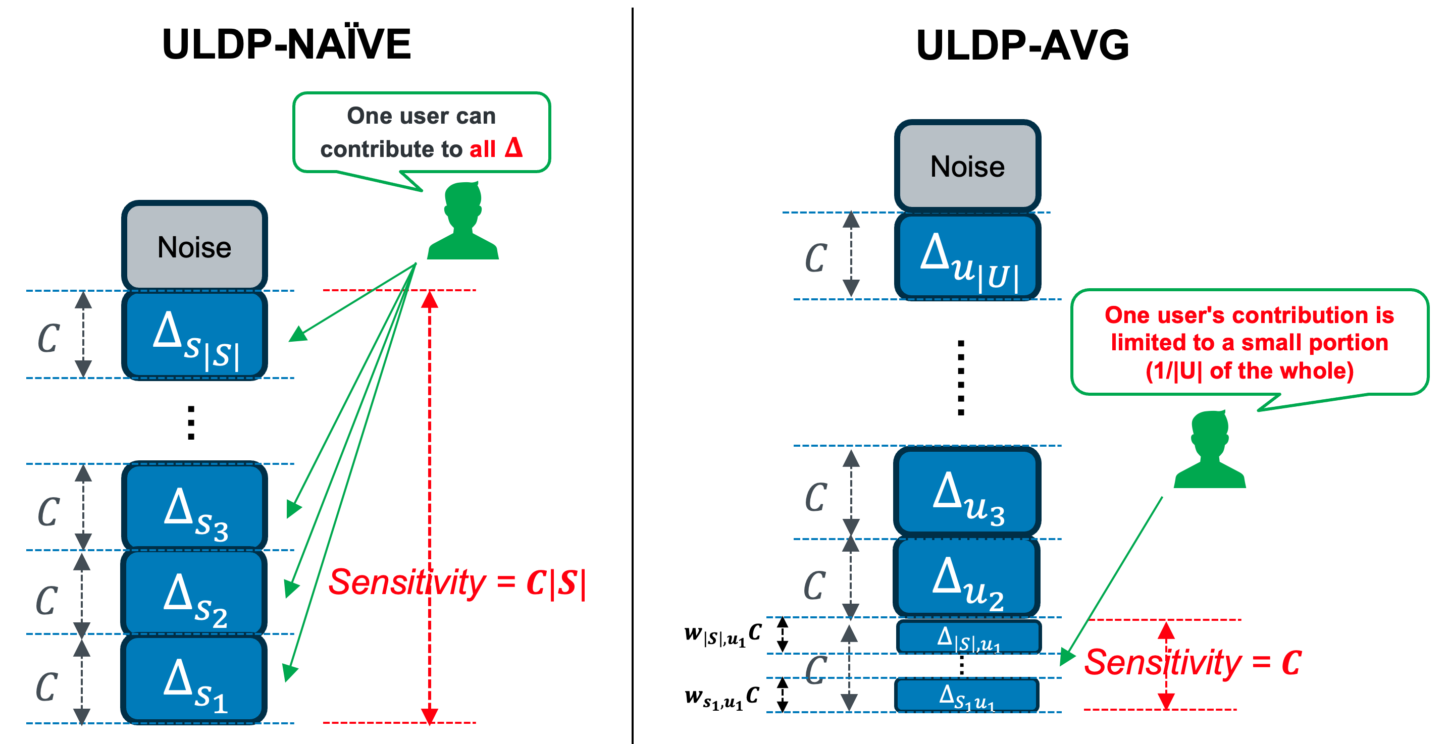
Figure 3. An intuitive illustration of the difference between ULDP-NAIVE and ULDP-AVG. In ULDP-NAIVE, every user can contribute to whole model deltas. In ULDP-AVG, one user’s contribution is limited to a small portion, i.e., $1/|U|$ of the whole model delta, which reduces user-level sensitivity.

Remark 2.

The first three terms recover the standard convergence bound up to constants for FedAVG (Yang et al., 2021) when considering participants in FL as user-silo pairs (i.e., we have $|S||U|$ participants). The asymptotic bound is $O(\frac{1}{\sqrt{|S||U|QT}}+\frac{1}{T})$. Theorem 6 achieves this when we choose the global and local learning rates $\eta_{g}=|S|\sqrt{|S||U|Q}$ and $\eta_{l}=\frac{1}{\sqrt{T}QL}$, respectively. This requires a learning rate $|S|$ times larger than the usual FedAVG with $|S||U|$ participants, which can be interpreted as coming from the constraint on the weights $W$. The fourth term is the convergence overhead due to Gaussian noise addition, and the last fifth and sixth terms are the overhead due to bias from the clippings. If both the noise and the clipping bias are zero, the convergence rate is asymptotically the same as the FedAVG convergence rate.

Remark 3.

The fourth term, accounting for the overhead due to noise, differs slightly from DP-FedAVG. This term is inversely proportional to $|S||U|^{2}$. As highlighted in the previous remark, if the global learning rate is set as $\eta_{g}=|S|\sqrt{|U|Q}$ in ULDP-AVG, this term becomes proportional to $\sqrt{|U|}/|U|^{2}$, consistent with the case of DP-FedAVG with $|U|$ participants.

Remark 4.

The fifth and sixth terms correspond to the overhead due to the clipping biases $\left|\alpha^{s,u}_{t}-\tilde{\alpha}^{s,u}_{t}\right|$ and $\left|\tilde{\alpha}^{s,u}_{t}-\bar{\alpha}_{t}\right|$, respectively. The quantity $\left|\alpha^{s,u}_{t}-\tilde{\alpha}^{s,u}_{t}\right|$ represents the local gradient variance across all users in all silos and can be made zero by full-batch gradient descent. The noteworthy term is $\left|\tilde{\alpha}^{s,u}_{t}-\bar{\alpha}_{t}\right|$. As discussed in the analysis of (Zhang et al., 2022), this term is influenced by the structure of the neural network and data heterogeneity. It roughly quantifies how much the magnitudes of all gradients deviate from the global mean. We may be able to minimize these values by selecting appropriate weights $\mathbf{W}$, guided by the following optimization problem:

$$\min_{\mathbf{W}}{\sum_{s\in S}\sum_{u\in U}\left|\tilde{\alpha}^{s,u}_{t}-\bar{\alpha}_{t}\right|},\;\text{s.t.,}\;w_{s,u}>0,\forall{u},\sum_{s\in S}{w_{s,u}}=1$$

$$\left(=\sum_{s\in S}\sum_{u\in U}\left|w_{s,u}C_{s,u}-\frac{1}{|S||U|}\sum_{s^{\prime}\in S}\sum_{u^{\prime}\in U}{w_{s^{\prime},u^{\prime}}C_{s^{\prime},u^{\prime}}}\right|\right)$$

where $C_{s,u}:=\frac{C}{\max{(C,\eta_{l}\lVert\mathbb{E}\left[\sum_{q\in[Q]}g^{s,u}_{t,q}\right]\rVert)}}$.

However, determining the optimal weights is challenging because we cannot predict the gradients’ norms in advance, which could also cause another privacy issue. In next section, we present a heuristic weighting strategy that aims to reduce this bias.

4. Enhanced Weighting and Private weighting protocol

4.1. The weighting protocol

In considering the bias described in Remark 4, we employed uniform clipping weights in the ULDP-AVG algorithm (Algorithm 3 Line 16), i.e., for any $s\in S$ and $u\in U$, we set $w_{s,u}=1/|S|$, as a simple solution without privacy violation. Now we propose an enhanced weighting strategy that aims to reduce the bias. We set a weight $w^{opt}_{s,u}$ for $C_{s,u}$ according to the number of records for user $u$ in silo $s$, following the heuristic that a gradient computed from a large number of records yields a better estimation that is closely aligned with the average. This results in smaller bias. That is, let $n_{s,u}$ be the number of records for user $u$ in silo $s$, we set the weight as follows:

(4) $$w^{opt}_{s,u}:=\frac{n_{s,u}}{\sum_{s\in|S|}{n_{s,u}}}.$$

We empirically demonstrate the effectiveness of this strategy later.

Private weighting protocol. Given the above weighting strategy that relies on number of user records per user per silo, the crucial question arises: how can this be implemented without violating privacy? A central server could aggregate histograms encompassing the user population (number of records per user) within each silo’s dataset. Subsequently, the server could compute the appropriate weights for each silo and distribute these weights back to the respective silos. However, it raises significant privacy concerns, since the histograms are directly shared with the server. Moreover, when the server broadcasts the weights back to the silos, it enables an estimation of the entire histogram of users across all the silos, posing a similar privacy risk against other silos. In essence, the privacy protection is necessary in both directions. This is challenging. Additive homomorphic encryption, such as Paillier cryptosystem, is often used for this situation (Alexandru and Pappas, 2022), but it is impossible to securely compute inverse values (for the weight in Eq. (4)). Note that unlimited records per user make DP impractical for protection.

To address this privacy issue, we design a novel private weighting protocol to securely aggregate the user histograms and also to securely perform local training and model aggregation. The protocol leverages well-established cryptographic techniques, including secure aggregation (Bonawitz et al., 2017; So et al., 2023), the Paillier cryptosystem (Alexandru and Pappas, 2022), and multiplicative blinding (Damgård et al., 2007). Intuitively, the protocol employs multiplicative blinding to hide user histograms against the server while allowing the server to compute inverses of blinded histograms to compute the weights (Eq. (4)). Subsequently, the server employs the Paillier encryption to conceal the inverses of blinded histograms because the silo knows the blinded masks. This enables the server and silos to compute private weighted sum aggregation with its additive homomorphic property.

Protocol 1 Private Weighting Protocol

Inputs: Silo $s\in S$ that holds an dataset with $n_{s,u}$ records for each user $u\in U$. $\mathcal{A}$ is central aggregation server. $N_{\text{max}}$ is upper bound on the number of records per user, e.g., 2000. $P$ is precision parameter, e.g, $10^{-10}$. $\lambda$ is security parameter, e.g., $3072$-bit security. (1) Setup. (a) $\mathcal{A}$ generates Paillier keypairs ($PK$, $SK$) with the given security parameter $\lambda$ and sends the public key $PK$ to all silos. All silos $s$ generate DH keypairs ($pk_{s}$, $sk_{s}$) with the same parameter $\lambda$ and transmit their respective public key $pk_{s}$ to $\mathcal{A}$. Both $\mathcal{A}$ and all silos compute $C_{\text{LCM}}$, which is the least common multiple of all integers up to $N_{\text{max}}$. The modulus $n$ included in $PK$ is used for the finite field $\mathbb{F}_{n}$ by $\mathcal{A}$ and all silos. (b) After receiving all $pk_{s}$, $\mathcal{A}$ broadcasts all DH public keys $pk_{s}$ to all $s$. All $s$ compute shared keys $sk_{s,s^{\prime}}$ from $sk_{s}$ and received public keys $pk_{s^{\prime}}$ for all $s^{\prime}\in S$. (c) Silo $0$ ($\in S$) generates a random seed $R$ and encrypts $R$ using $sk_{0,s^{\prime}}$ to obtain $Enc(R)$ and sends $Enc(R)$ to $s^{\prime}$ via $\mathcal{A}$ for all $s^{\prime}$. All $s\in S\setminus 0$ receive and decrypt $Enc(R)$ with $sk_{s,0}$ and get $R$ as a shared random seed. (d) All $s$ generate multiplicative blind masks $r_{u}\in\mathbb{F}_{n}$ with the same $R$ and compute blinded histogram as $B(n_{s,u})\equiv r_{u}n_{s,u}\,(\mathrm{mod}\,n)$ for all $u\in U$. (e) All $s$ generate pair-wise additive masks $r^{u}_{s,s^{\prime}}\in\mathbb{F}_{n}$ employing $sk_{s,s^{\prime}}$ for all $s^{\prime}$ and $u$, with $r^{u}_{s,s^{\prime}}=r^{u}_{s^{\prime},s}$. Subsequently, they calculate the doubly blinded histogram as $B^{\prime}(n_{s,u})\equiv B(n_{s,u})+\sum_{s<s^{\prime}}{r^{u}_{s,s^{\prime}}}-\sum_{s>s^{\prime}}{r^{u}_{s,s^{\prime}}}\,(\mathrm{mod}\,n)$. All $s$ send $B^{\prime}(n_{s,u})$ to $\mathcal{A}$. $\mathcal{A}$ aggregates these contributions to compute $B(N_{u})\equiv\sum_{s\in S}{B^{\prime}(n_{s,u})}\,(\mathrm{mod}\,n)$ for each $u$, denoting $N_{u}=\sum_{s\in S}{n_{s,u}}$. (f) $\mathcal{A}$ computes the inverse of $B(N_{u})$ as $B_{\text{inv}}(N_{u})=B(N_{u})^{-1}$ for each $u$. This is the multiplicative inverse on $\mathbb{F}_{n}$, which is efficiently computed by the Extended Euclidean algorithm. (2) Weighting for each training round $t$. (a) $\mathcal{A}$ encrypts $B_{\text{inv}}(N_{u})$ using Paillier’s public key $PK$, resulting in $Enc_{\text{p}}(B_{\text{inv}}(N_{u}))$ for all $u$. If user-level sub-sampling is required, the server performs Poisson sampling with a given probability $q$ for each user before the encryption. For non-selected users, $B_{\text{inv}}(N_{u})$ is set to 0. If we require user-level sub-sampling, we perform Poisson sampling with given probability $q$ on the server for each user before the Paillier’s encryption and set $B_{\text{inv}}(N_{u})=0$ for all users not selected. Subsequently, $\mathcal{A}$ broadcasts all $Enc_{\text{p}}(B_{\text{inv}}(N_{u}))$ to all silos. (b) In each $s$, following the approach of ULDP-AVG, the clipped model delta $\tilde{\Delta}^{s,u}_{t}$ is computed for each user $u$. The weighted clipped model delta is then calculated as $\displaystyle Enc_{\text{p}}$ $\displaystyle(\tilde{\Delta}^{s,u}_{t})=$ Encode $\displaystyle(\tilde{\Delta}^{s,u}_{t},P,n)n_{s,u}r_{u}C_{\text{LCM}}Enc_{\text{p}}(B_{\text{inv}}(N_{u})).$ Let the Gaussian noise be $z^{s}_{t}$, we then compute $z^{\prime}_{s}=\textsc{Encode}(z^{s}_{t},P,n)C_{\text{LCM}}$. Note that we need to approximate real number $\tilde{\Delta}^{s,u}_{t}$ and $z^{s}_{t}$ on a finite field using Encode (described in Algorithm 5). Lastly, we compute the summation $Enc_{\text{p}}(\Delta^{s}_{t})=\sum_{u\in U}{Enc_{\text{p}}(\tilde{\Delta}^{s,u}_{t})}+z^{\prime}_{s}$. (c) In each $s$, random pair-wise additive masks are generated, and secure aggregation is performed on $Enc_{\text{p}}(\Delta^{s}_{t})$ mirroring the steps in 1.(f). Then, $\mathcal{A}$ gets $\sum_{s\in S}{Enc_{\text{p}}(\Delta^{s}_{t})}$. $\mathcal{A}$ decrypts it with Paillier’s secret key $SK$ and decodes it by Decode$(\sum_{s\in S}{\Delta^{s}_{t}},P,C_{\text{LCM}},n)$ and recovers the aggregated value. (d) Steps 2.(a) through 2.(c) are repeated for each training round.

Algorithm 5 Encode and Decode

1:procedure Encode($x,P,n$) $\triangleright$ e.g., $P=10^{-10}$

2:     /* to turn floating point into fixed point */

3:     $x\leftarrow x/P$ $\triangleright$ compute as floating point

4:     $x\leftarrow x$ as integer

5:     $x\leftarrow x\,(\mathrm{mod}\,n)$ $\triangleright$ to map integer $\mathbb{Z}$ into finite field $\mathbb{F}_{n}$

6:     return $x$

7:procedure Decode($x,P,C_{\text{LCM}},n$)

8:     /* to map finite field $\mathbb{F}_{n}$ number into integer $\mathbb{Z}$ */

9:     if $x>n//2$ then $\triangleright$ $//$ means integer division

10:         $x\leftarrow x-n$

11:     else

12:         $x\leftarrow x$      

13:     /* compute as floating point */

14:     $x\leftarrow x/C_{\text{LCM}}$ $\triangleright$ to remove $C_{\text{LCM}}$ factor

15:     $x\leftarrow xP$ $\triangleright$ to recover original magnitude

16:     return $x$

The details of the private weighting protocol are explained in Protocol 4.1. The protocol consists of a setup phase, which is executed only once during the entire training process, and a weighting phase, which is executed in each round of training. In the setup phase, as depicted in (a-c) of Protocol 4.1, the server generates a key-pair for Paillier encryption, while the silos establish shared random seeds through a Diffie–Hellman (DH) key exchange via the server. Subsequently, in steps of (d-f), the blinded inverses of the user histogram are computed. In the weighting phase, (a) the server prepares the encrypted weights, (b) the silos compute user-level weighted model deltas in the encrypted world, and (c) the server recovers the aggregated value. It is important to note that in the Paillier cryptosystem, the plaintext $x$ exists within the additive group modulo $n$, while encrypted data (denoted as $Enc_{\text{p}}(x)$) belongs to the multiplicative group modulo $n^{2}$ with an order of $n$. The system allows for operations such as addition of ciphertexts and scalar multiplication and addition on ciphertexts.

Private user-level sub-sampling. Note that our assumption so far is that the results of user-level sub-sampling (i.e., whether a user is sampled) are open to the aggregation server. This is also the case in Protocol 4.1. However, it could be hidden by combining the two-party verifiable sampling scheme with 1-out-of-P Oblivious Transfer (OT) as described in (Kato et al., 2021). As an overview, for each user $u$, the server creates $P-1$ dummy data $Enc_{\text{p}}(0)$ for $Enc_{\text{p}}(B_{\text{inv}}(N_{u}))$ described in the step 2.(a) of Protocol 4.1. When the client performs OT on this data, the selection probability of $Enc_{\text{p}}(B_{\text{inv}}(N_{u}))$ is $\frac{1}{P}$ and that of $Enc_{\text{p}}(0)$ is $\frac{P-1}{P}$. The selection of $Enc_{\text{p}}(B_{\text{inv}}(N_{u}))$ means that the user is not sampled by the user-level sub-sampling. In this way, the server does not know which data was retrieved by the client from the OT, and the client cannot know the sampling result due to the Paillier encryption. However, the expressed probability is likely to be less strict because it can only represent discrete probability distributions. This process requires extra computational costs for both the server and the silo, proportional to the number of users, and should not be included if it is not necessary.

4.2. Theoretical analysis

We provide a theoretical analysis of this private weighting protocol (Protocol 4.1) in terms of correctness and privacy.

Correctness. The protocol must compute the correct result that is the same as non-secure method. To this end, we consider the correctness of the aggregated data obtained in each round.

Theorem 1 (Correctness of Protocol 4.1).

Let $\sum_{s\in S}\Delta^{s}_{t}$ with non-secure method be $\Delta$ and the one with the Protocol 4.1 be $\Delta_{\text{sec}}$, our goal is formally stated as $\Pr[|\Delta-\Delta_{\text{sec}}|_{\infty}>P]<negl$, where $P$ is a precision parameter and $negl$ signifies a negligible value.

Privacy. In the protocol, both the central server and the silos do not get more information than what is available in the original ULDP-AVG while we perform the enhanced weighting strategy.

Theorem 2 (Privacy of Protocol 4.1).

None of the parties learns $n_{s,u}$ other than their own users from the protocol.

5. Experiments

5.1. Settings

In this section, we evaluate the privacy-utility trade-offs of the proposed methods (ULDP-AVG/SGD), along with the baselines (ULDP-NAIVE/GROUP-$k$) and a non-private baseline (FedAVG with two-sided learning rates (Yang et al., 2021), denoted by DEFAULT). In ULDP-AVG/SGD, we set the weights as $w_{s,u}=1/|S|$ for all $s$ and $u$, the one using $w^{opt}_{s,u}$ is referred to as ULDP-AVG-w. Regarding ULDP-GROUP-$k$, flags $\mathbf{B}$ are generated for existing records to minimize waste on filtered out records, despite the potential privacy concerns. Various values, including the maximum number of user records, the median, 2, and 8, are tested as group size $k$ and we report GDP using group-privacy conversion of RDP. In cases where $k$ is not a power of 2, the computed $\epsilon$ is reported for the largest power of 2 below $k$, showcasing the lower bound of GDP to underscore that $\epsilon$ is large. The hyperparameters, including global and local learning rates $\eta_{g}$, $\eta_{l}$, clipping bound $C$, and local epoch $Q$, are set individually for each method. Execution times are measured on macOS Monterey v12.1, Apple M1 Max Chip with 64GB memory with Python 3.9 and 3072-bit security. Most of the results are averaged over 5 runs and the colored area in the graph represents the standard deviation. All of our implementations and experimental settings are available.

5.1.1. Datasets

Datasets used in the evaluation comprise real-world open datasets, including Credicard (Kaggle, 2018), well-known image dataset MNIST, and two benchmark medical datasets for cross-silo FL (Ogier du Terrail et al., 2022), HeartDisease and TcgaBrca. Creditcard is a tabular dataset for credit card fraud detection from Kaggle. We undersample the dataset and use about 25K training data and a neural network with about 4K parameters. For MNIST, we use a CNN with about 20K parameters, 60K training data and 10K evaluation data, and assigned silos and users to all of the training data. For HeartDisease and TcgaBrca, we use the same setting such as number of silos (4 and 6), data assignments to the silos, models, etc. as shown in (Ogier du Terrail et al., 2022). These two datasets are small and the model has less than 100 parameters.

For all datasets, we need to link all records to each user and silo. We allocate the records to users and silos as follows.

Record allocation for MNIST and Creditcard. We designed two different record distribution patterns, uniform and zipf, to model how user records are scattered across silos in the MNIST and Creditcard datasets. Both distributions take the number of users $|U|$ and the number of silos $|S|$. It associates each record with a user and a silo. (1) In uniform, every record is assigned to a user with equal probability, and likewise, each record is assigned to a silo with equal probability. (2) zipf combines two types of Zipf distributions. First, the distribution of the number of records per user follows a Zipf distribution. Then, for each user, the numbers of records are assigned to different silos based on another Zipf distribution. Each of the two Zipf distributions takes a parameter $\alpha$ that determines the concentration of the numbers. In the experiments, we used $\alpha=0.5$ for the first distribution and $\alpha=2.0$ for the second distribution. This choice is rooted in the observation that the concentration of user records is not as high as the concentration in the silos selected by each user. For Creditcard and MNIST, the number of silos $|S|$ is fixed at 5. We used 100, 1000 for Creditcard as $|U|$ and 100, 10000 for MNIST. For MNIST, we can require each user to have only 2 labels at most for non-i.i.d.

Record allocation for HeartDisease and TcgaBrca. For the HeartDisease and TcgaBrca datasets, we adopted the same two distributions uniform and zipf as the above-mentioned ones. In the benchmark datasets HeartDisease and TcgaBrca, all records are already allocated to silos and the number of records of each silo is fixed. Therefore, the design of the user-record allocation is slightly different. (1) In uniform, all records belong to one of the users with equal probability without allocation to silos. (2) In zipf, the number of records for a user is first generated according to a Zipf distribution, and 80% of the records are assigned to one silo, and the rest to the other silos with equal probability. The priority of the silo is chosen randomly for each user. We used $\alpha=0.5$ for the parameter of the Zipf. In TcgaBrca, Cox-Loss is used for loss function (Ogier du Terrail et al., 2022), which needs more than two records for calculating valid loss and we set more than two records for each silo and user for per-user clipping of ULDP-AVG.

5.2. Results

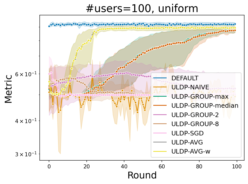
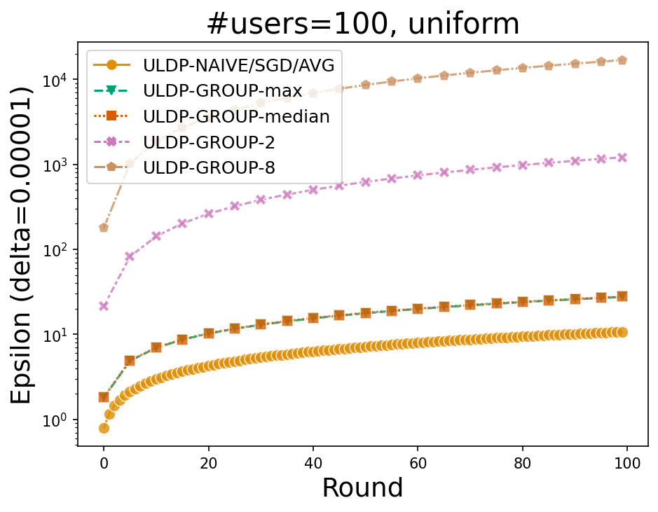
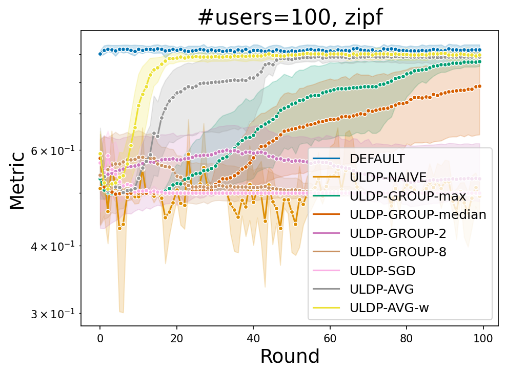
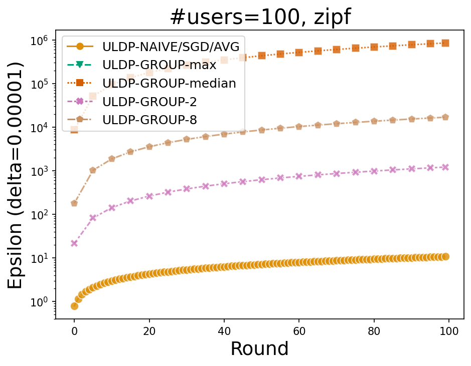
(a) $n\approx 246$ ($|U|=100$), uniform.

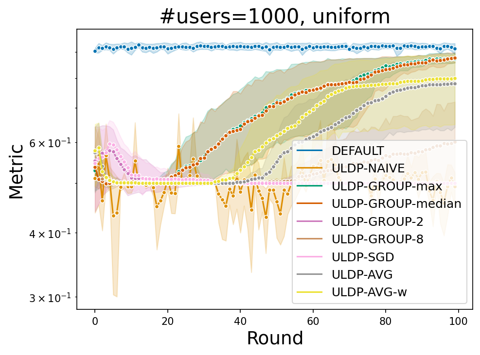
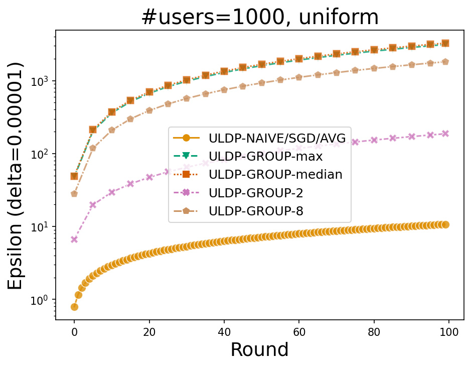
(b) $n\approx 246$ ($|U|=100$), zipf.

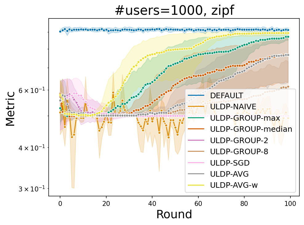
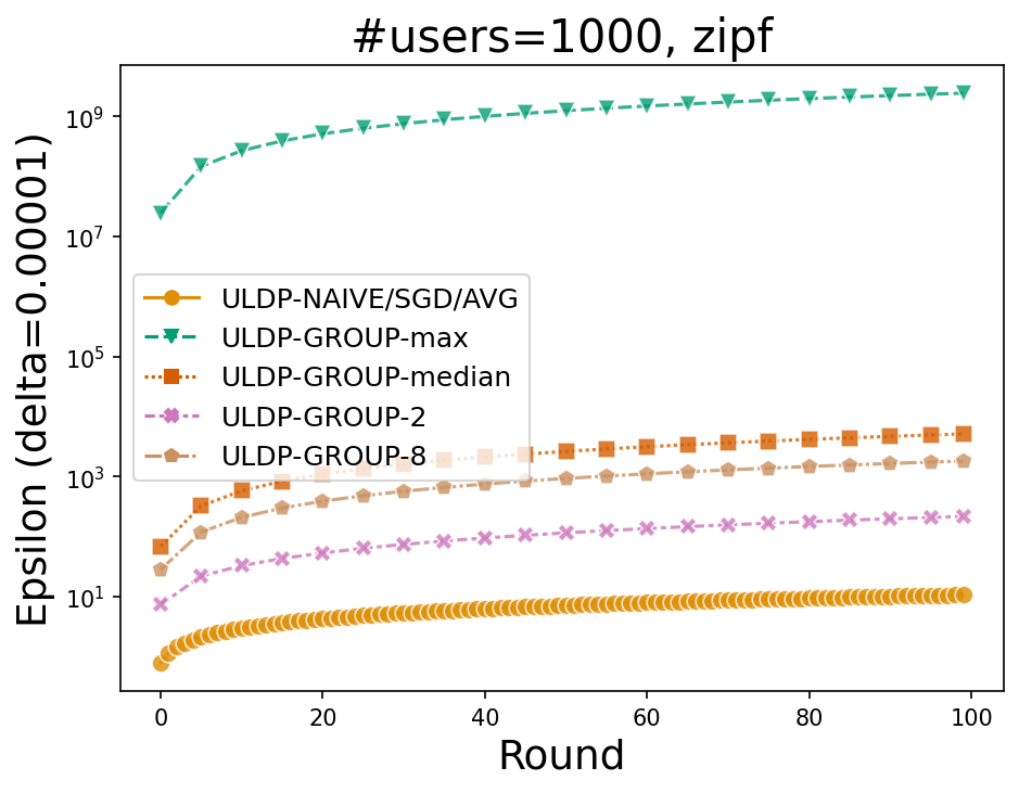
(c) $n\approx 25$ ($|U|=1000$), uniform.

(d) $n\approx 25$ ($|U|=1000$), zipf.

Figure 4. Privacy-utility trade-offs on Creditcard dataset: Test Accuracy (Left), Privacy (Right).

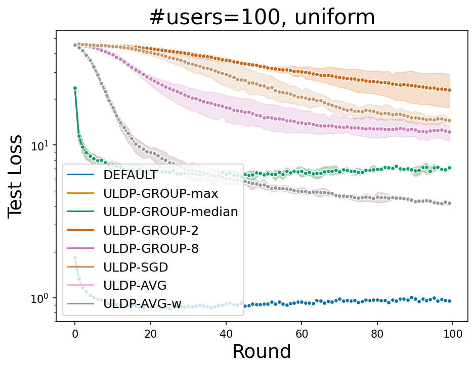
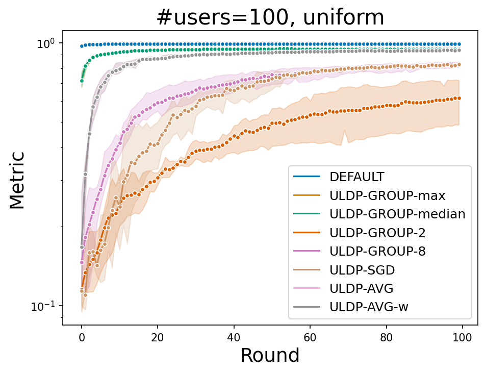
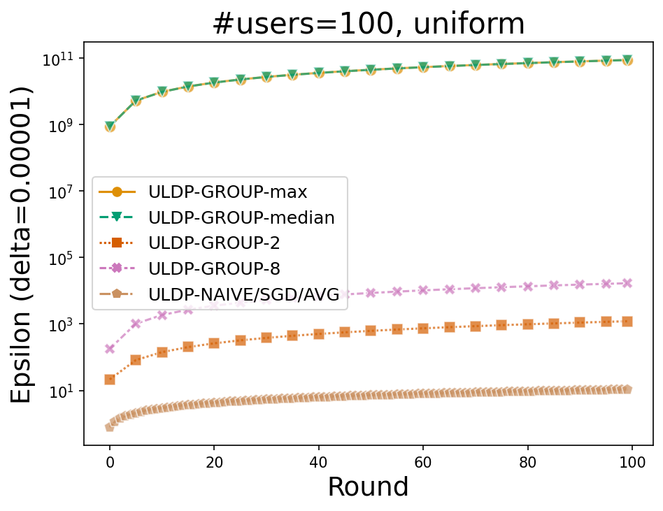
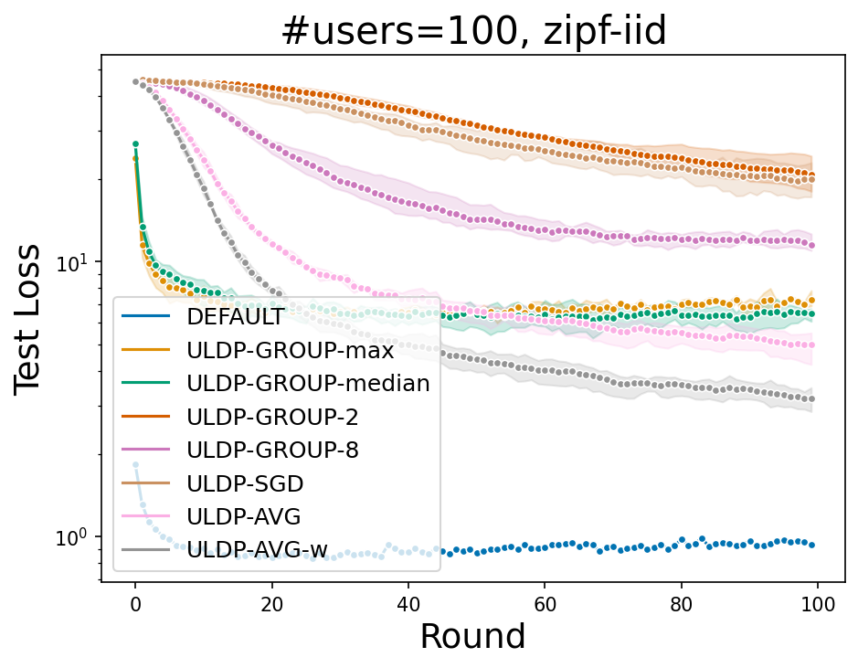
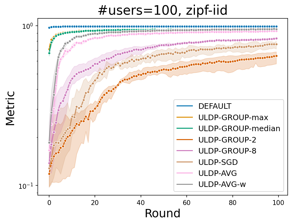
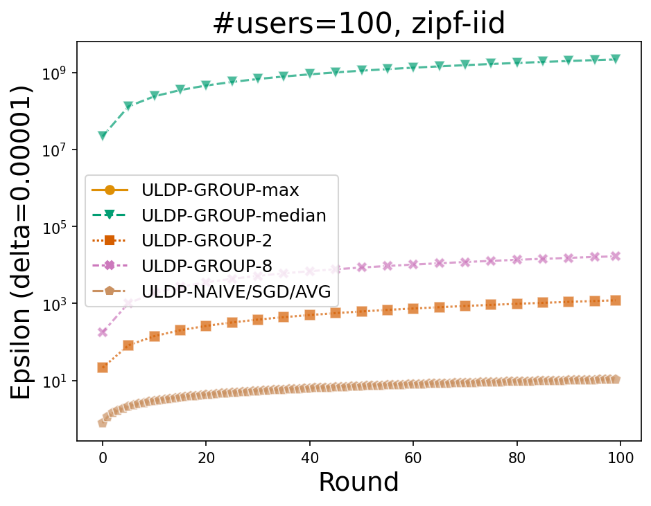
(a) $n\approx 600$ ($|U|=100$), uniform.

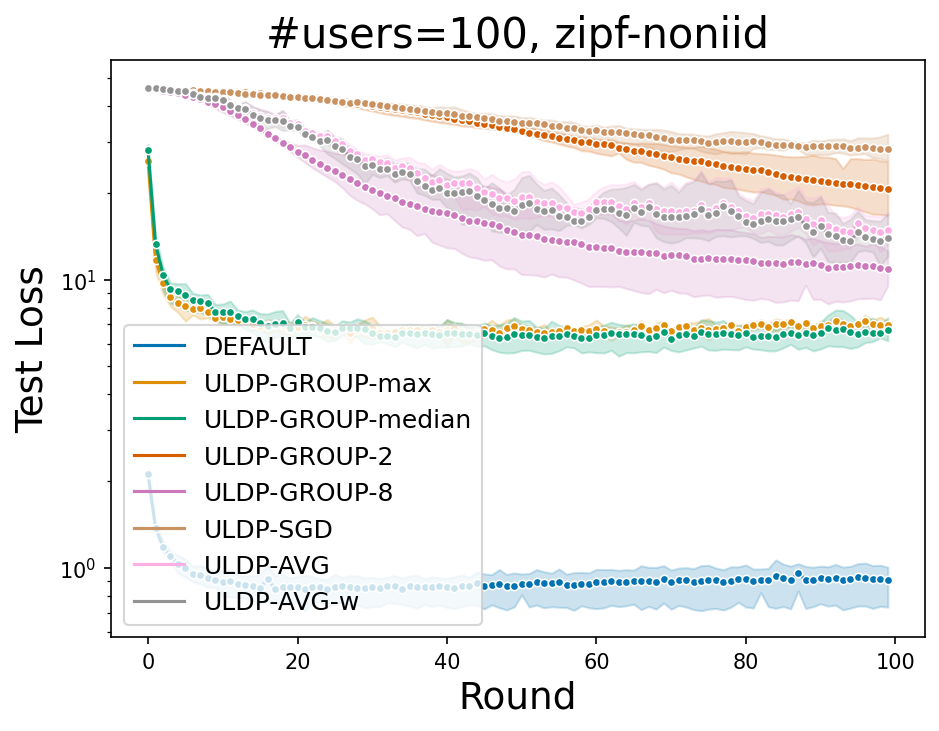
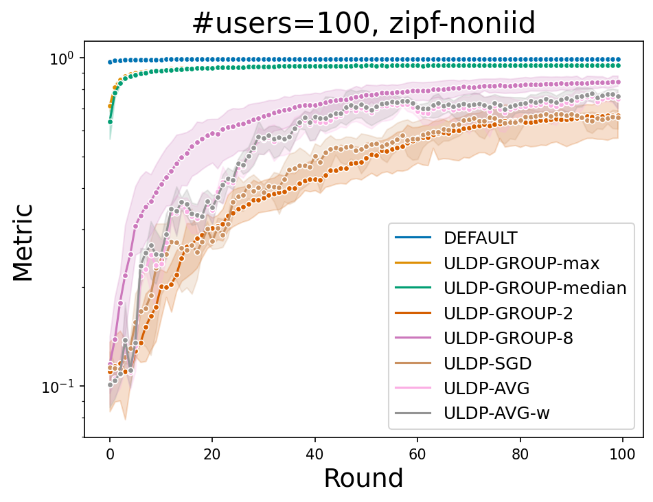
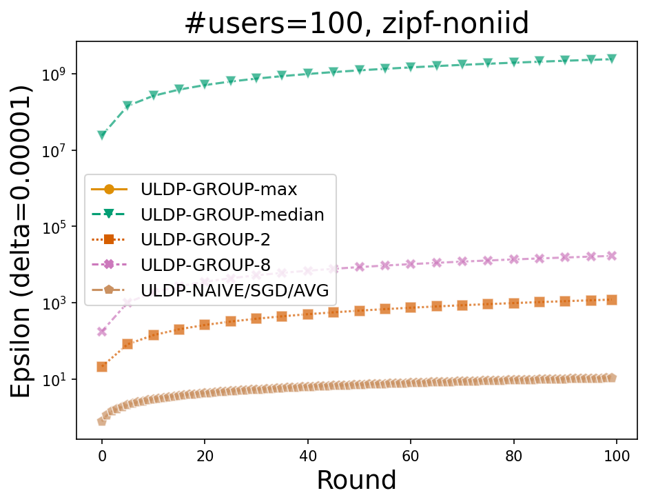
(b) $n\approx 600$ ($|U|=100$), zipf, iid.

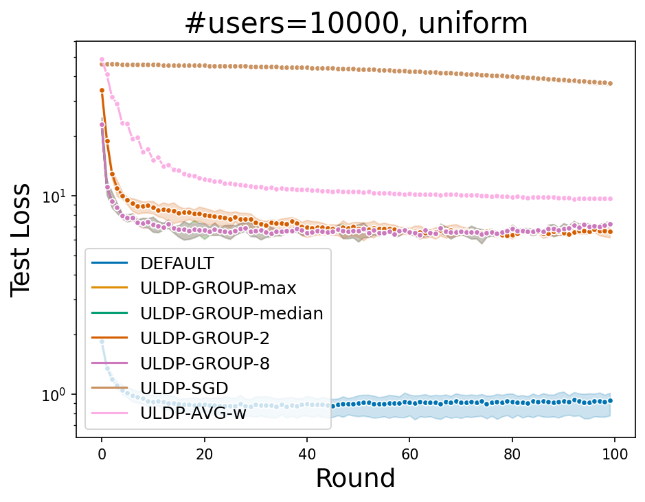
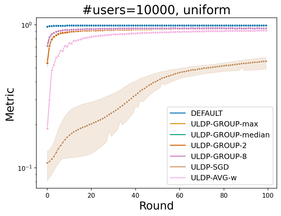
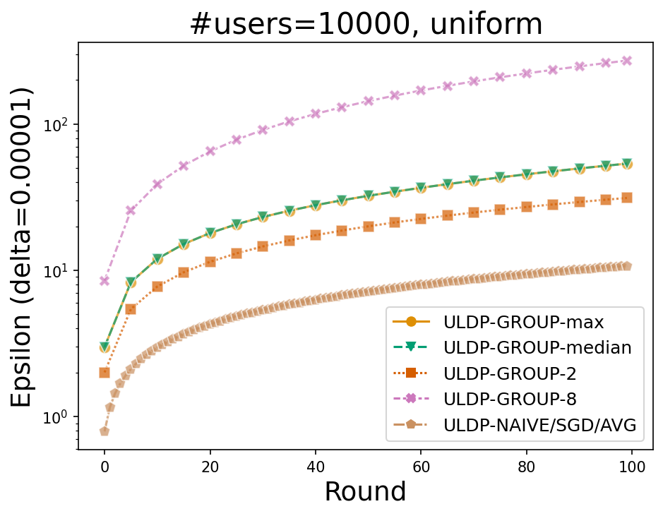
(c) $n\approx 600$ ($|U|=100$), zipf, non-iid.

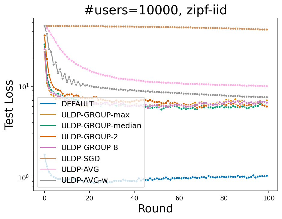
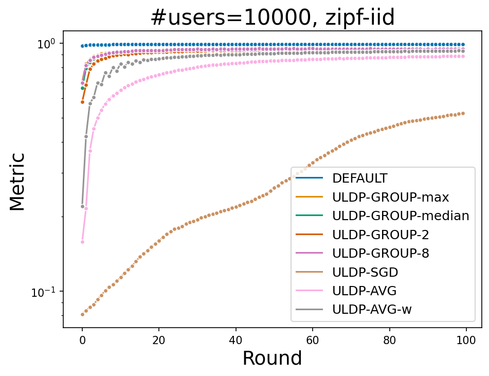
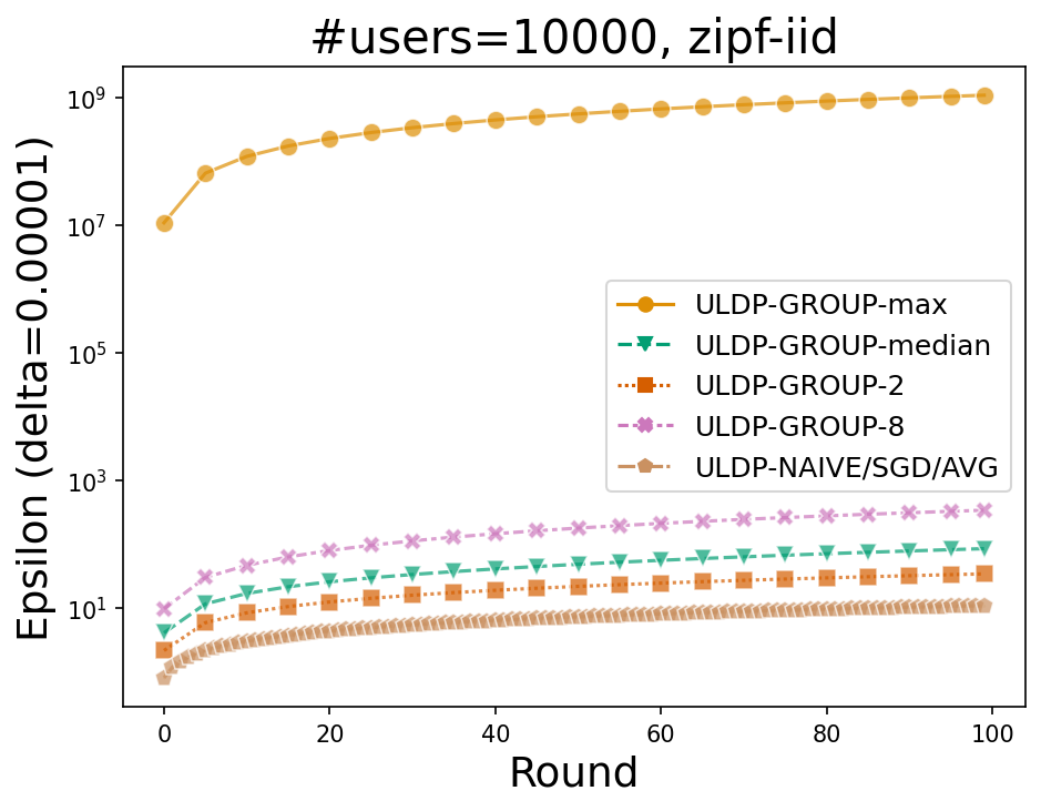
(d) $n\approx 6$ ($|U|=10000$), uniform, iid.

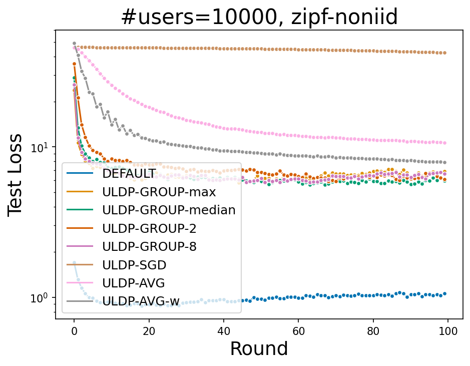
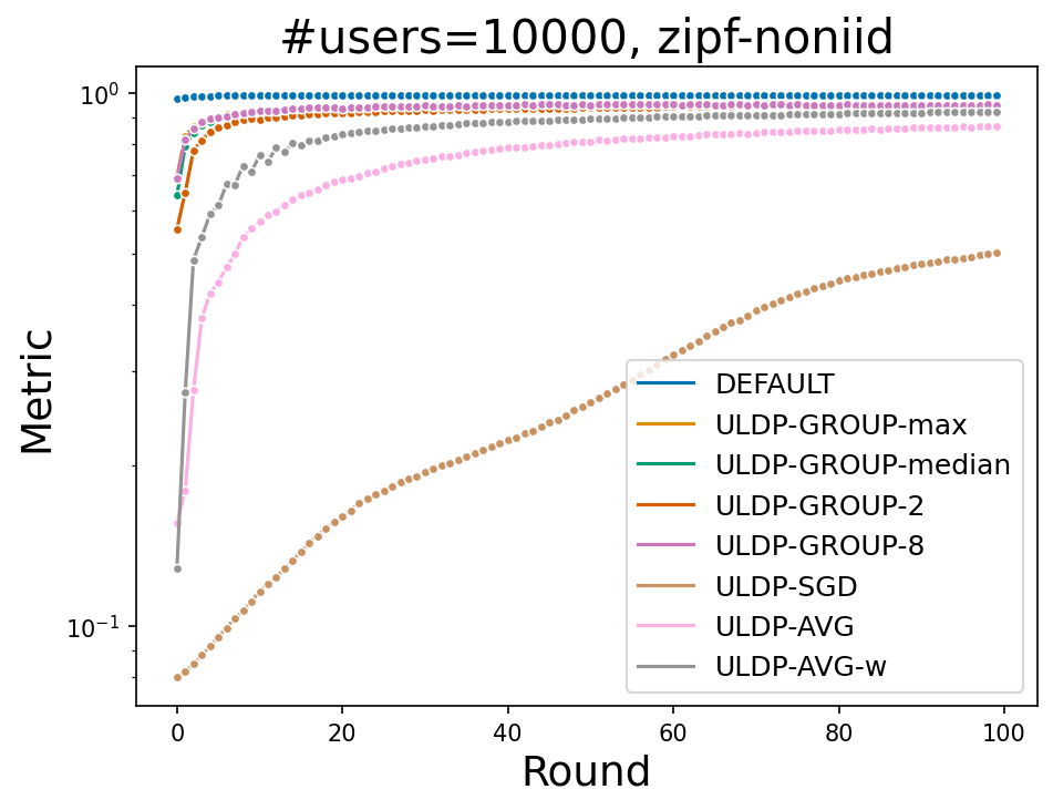
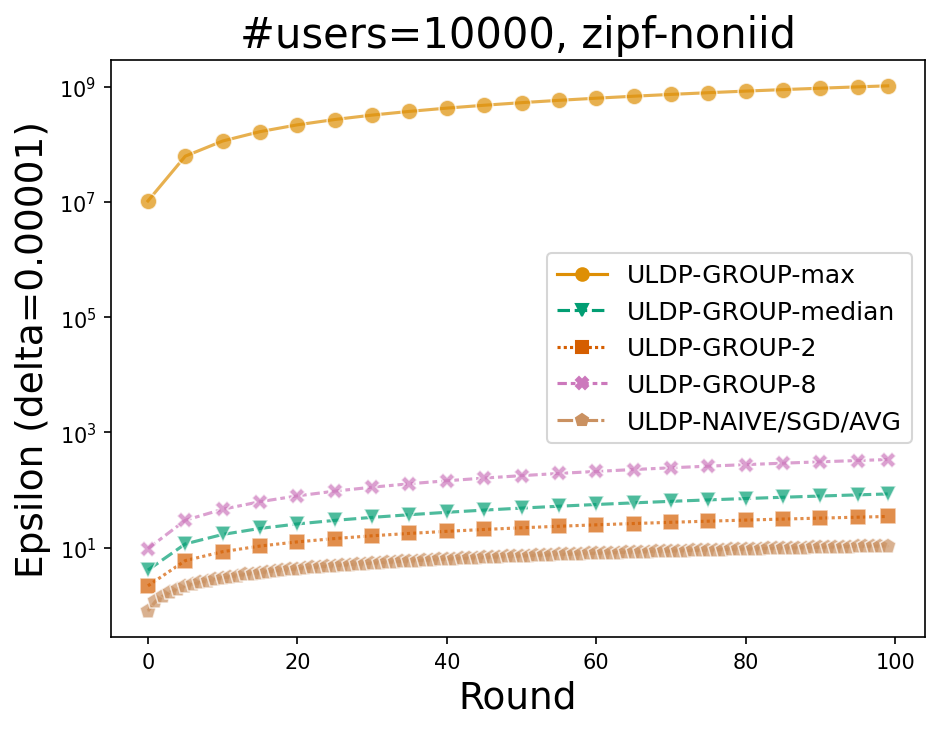
(e) $n\approx 6$ ($|U|=10000$), zipf, iid.

(f) $n\approx 6$ ($|U|=10000$), zipf, non-iid.

Figure 5. Privacy-utility trade-offs on MNIST dataset: Test Loss (Left), Accuracy (Middle), Privacy (Right).

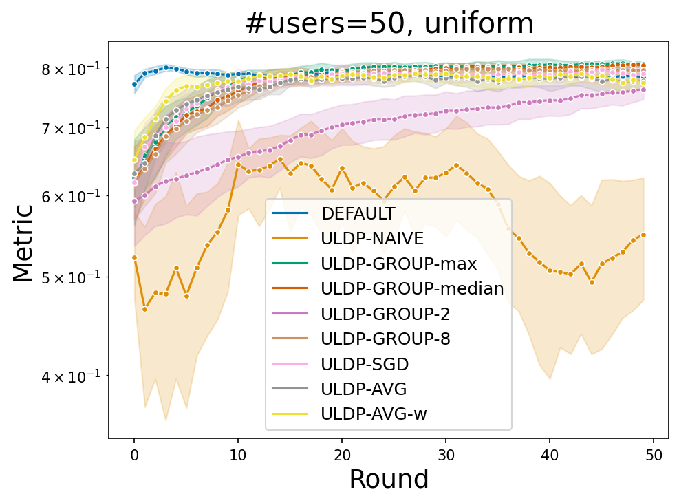
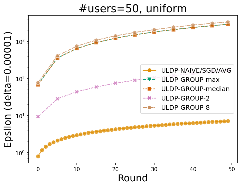
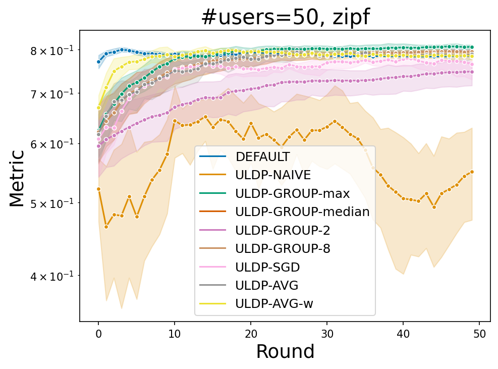
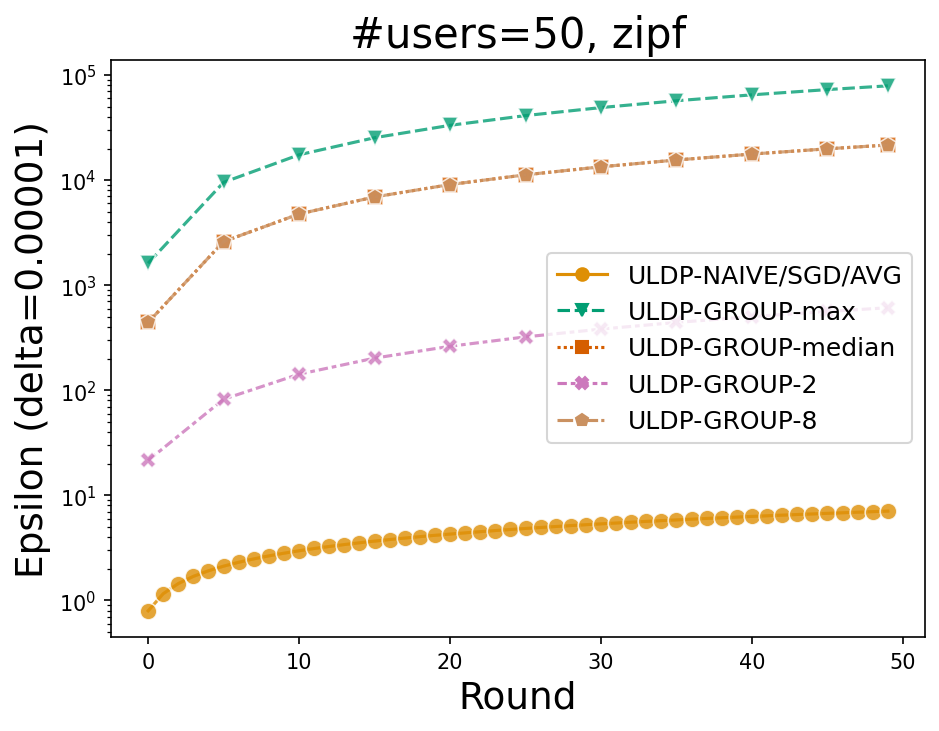
(a) $n\approx 10$ ($|U|=50$), uniform.

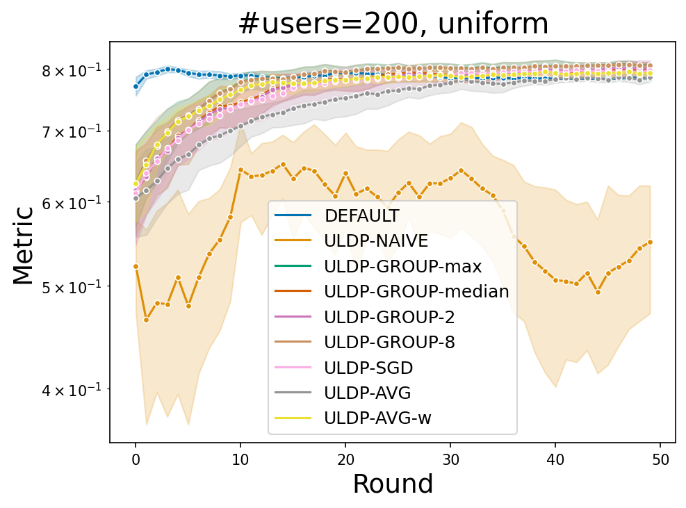
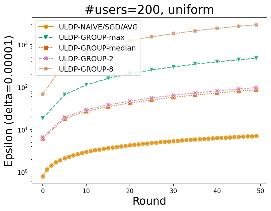
(b) $n\approx 10$ ($|U|=50$), zipf.

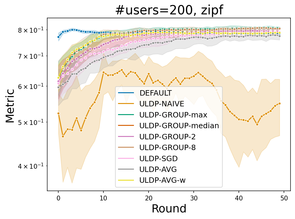
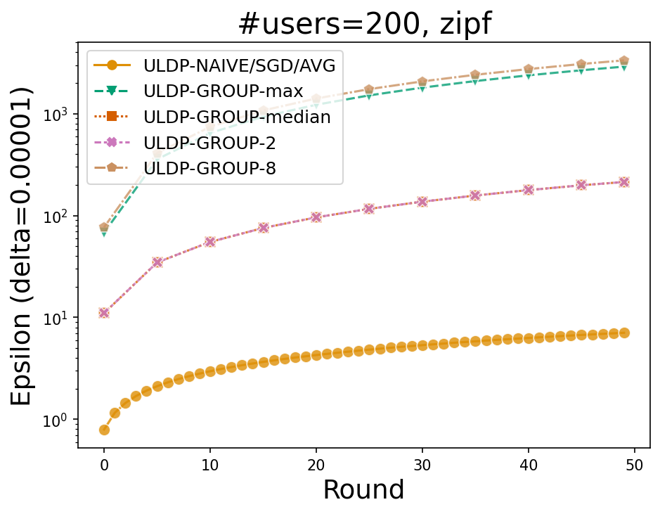
(c) $n\approx 2.5$ ($|U|=200$), uniform.

(d) $n\approx 2.5$ ($|U|=200$), zipf.

Figure 6. HeartDisease.

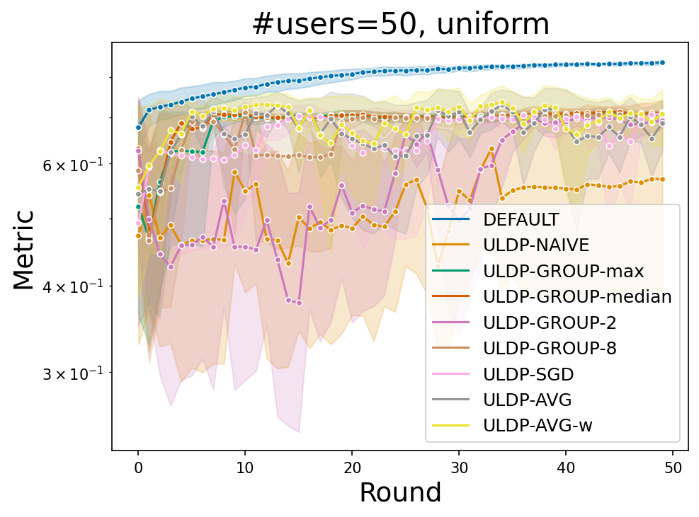
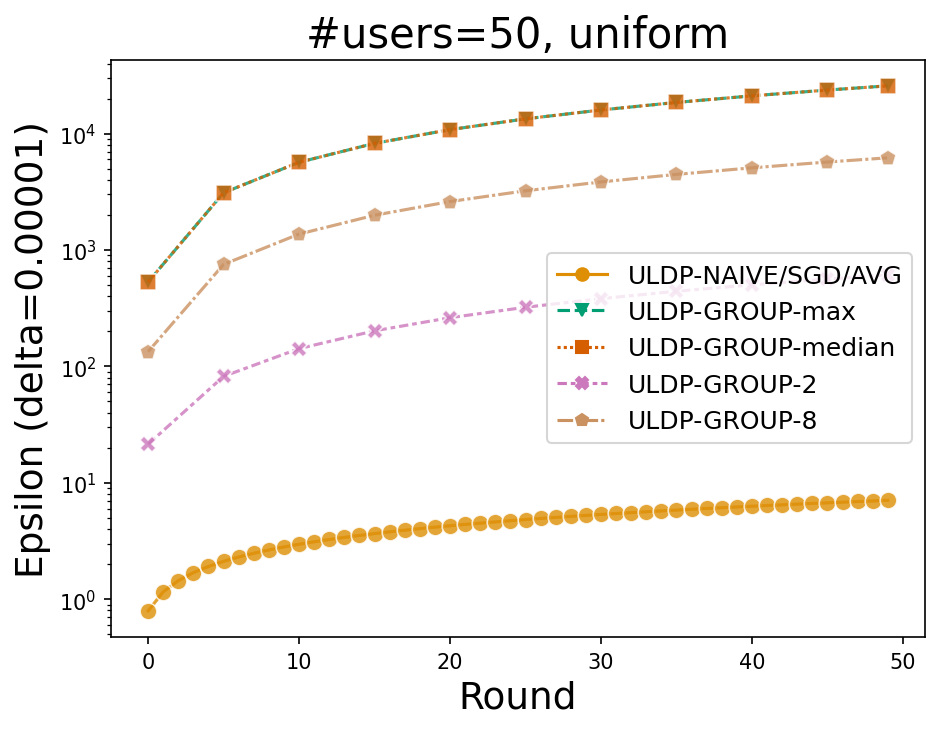
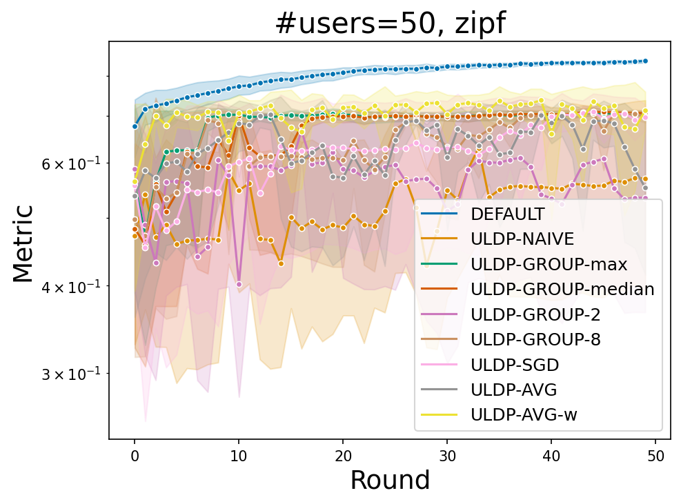
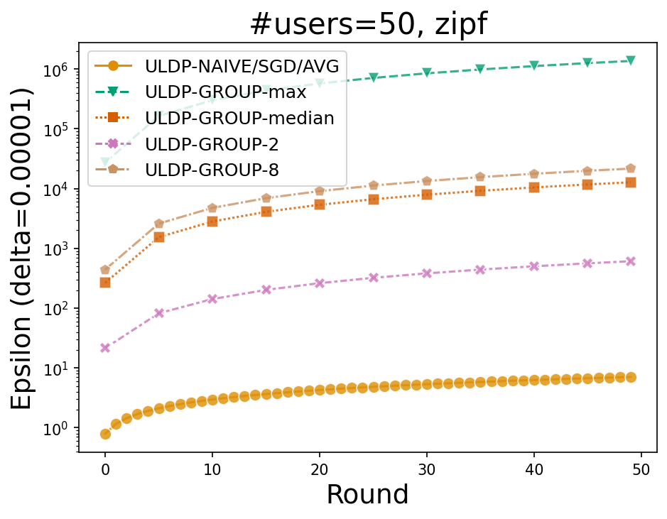
(a) $n\approx 17$ ($|U|=50$) uniform.

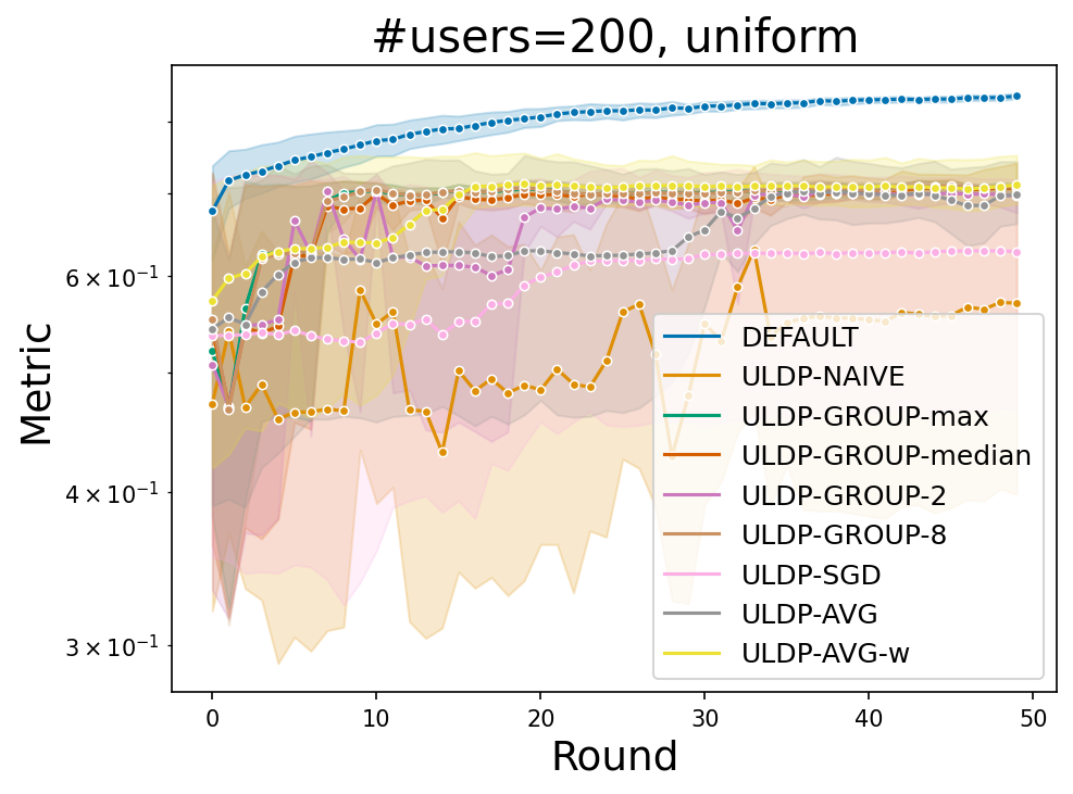
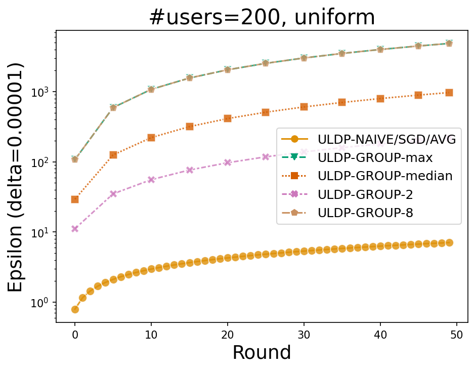
(b) $n\approx 17$ ($|U|=50$), zipf.

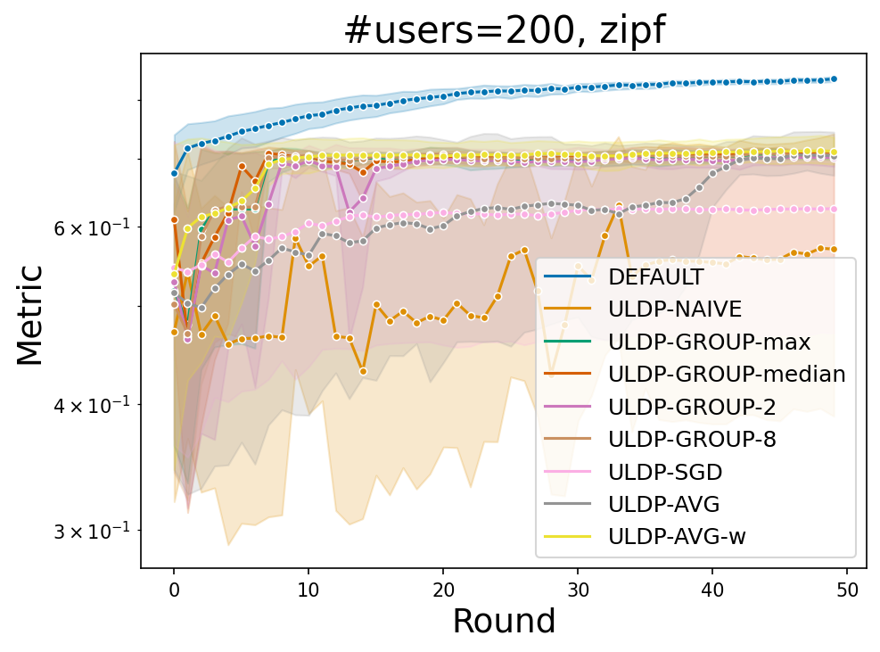
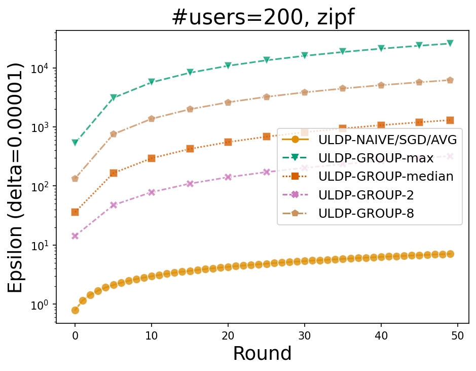
(c) $n\approx 4$ ($|U|=200$), uniform.

(d) $n\approx 4$ ($|U|=200$), zipf.

Figure 7. TcgaBrca.

Privacy-utility trade-offs under ULDP. Figures 4 show the utility and privacy evaluation results on Creditcard. The average number of records per user (denoted as $n$) in entire silos and the distribution changes for each figure. All experiments used a fixed noise parameter $\sigma=5.0$ and $\delta=10^{-5}$, utility metrics (Accuracy for Creditcard) are displayed on the left side and accumulated privacy consumption $\epsilon$ for ULDP are depicted on the right side. Note that the privacy bounds for ULDP-GROUP-$k$ are derived from the local DP-SGD and depend on not only the group size $k$ but also the size of the local training dataset.

Overall, the proposed method ULDP-AVG/SGD achieves competitive utility with fast convergence and high accuracy, while achieving considerably small privacy bounds, which means the significantly better privacy-utility trade-offs compared to baselines. We observe that the baseline method, ULDP-NAIVE, has low accuracy and that ULDP-GROUP-$k$ requires much larger privacy budgets, which is consistent with the analysis on the conversion of group privacy described earlier. The convergence speed of ULDP-AVG is faster than that of ULDP-SGD, which is the same as that of DP-FedAVG/SGD. Nevertheless, there is still a gap between ULDP-AVG and the non-private method (DEFAULT) in terms of convergence speed and ultimately achievable accuracy, as a price for privacy. Also, as shown in Figure 4(d), for small $n$ (i.e., a large number of users), ULDP-GROUP-max/median show higher accuracy than ULDP-AVG. This is likely due to the overhead from finer datasets at user-level, which increases the bias compared to DP-FedAVG, as seen in the theoretical convergence analysis for ULDP-AVG.

Figure 6, 7, and 5 show privacy-utility trade-offs on HeartDisease, TcgaBrca, and MNIST, respectively. All experiments used a fixed noise parameter (noise multiplier) $\sigma=5.0$ and $\delta=10^{-5}$, utility metrics (Accuracy for HeartDisease and MNIST, C-index for TcgaBrca) are plotted on the left side, and accumulated privacy consumption $\epsilon$ for ULDP are plotted on the right side. For clarity, the test loss is shown on the left-hand side for MNIST. The average number of records per user (denoted as $n$) in entire silos and the distribution (uniform/zipf) changes for each figure.

In all datasets, consistently, ULDP-AVG is competitive in terms of utility, ULDP-AVG-w shows much faster convergence, and ULDP-SGD shows slower convergence. ULDP-NAIVE achieves a low privacy bound; however, its utility is much lower than other methods. ULDP-GROUP-$k$ show reasonably high utility, especially in settings where $n$ is small. This is because the records to be removed due to the number of records per user being over group size $k$ is small. However, the ULDP privacy bound ULDP-GROUP-$k$ achieves ends up being very large. Note that the privacy bounds for ULDP-GROUP-$k$ are derived from the local DP-SGD and depend on not only the group size $k$ but also the size of the local training dataset. The exceptions are cases where the local data set size is large and the number of records per user is very small as in Figures 5(f), 5(f), and 5(f). In these cases, ULDP-GROUP-2 achieves a reasonably small privacy bound. In other words, if the number of user records is fixed at one or two in the scenario, and the number of training records is large (it is advantageous for ULDP-GROUP because the record-level sub-sampling rate in DP-SGD becomes small), it could be better to use ULDP-GROUP.

Effect of non-IID data. The results for the MNIST, non-i.i.d, and $|U|=100$ case highlight a weak point of ULDP-AVG. Note that non-i.i.d here is at user-level and DEFAULT and ULDP-GROUP are less affected by non-i.i.d because they train per silo rather than per user. As Figure 5(f) shows, the convergence of ULDP-AVG is worse compared to other results. It suggests that ULDP-AVG may emphasize the bad effects of user-level non-i.i.d. distribution that were not an issue with normal cross-silo FL because the gradient is not computed at the user level as in ULDP-AVG. On the other hand, this is less problematic when the number of users is large as shown in Figure 5(f). This is due to the relatively smaller effect of individual user overfitting caused by non-i.i.d. distribution as the number of users increases.

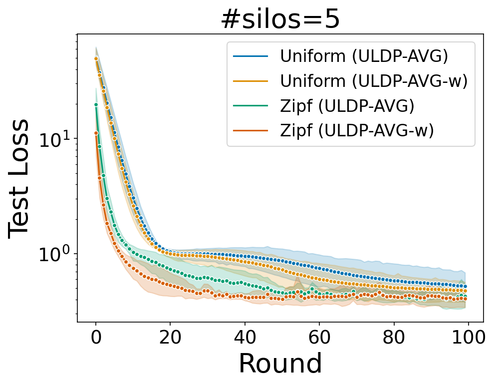
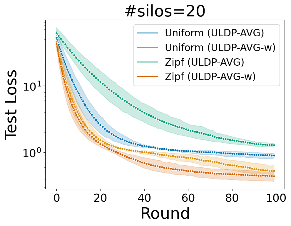
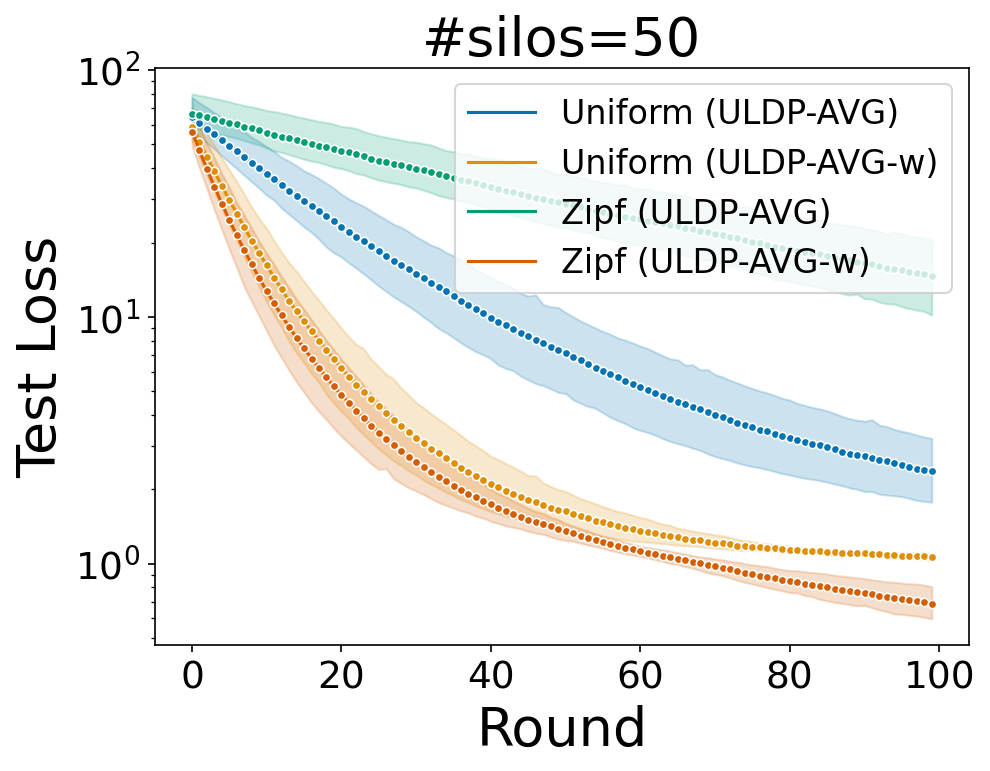
Figure 8. Test loss of Creditcard: Weighting method is effective, especially in skewed distribution in many silos.

Effectiveness of enhanced weighting strategy. To highlight the effectiveness of the enhanced weighting strategy, Figure 8 shows the test losses of the Creditcard dataset on different record distributions with ULDP-AVG and ULDP-AVG-w. We present the results with various numbers of silos: 5, 20, and 50. The need for the better weighting strategy is emphasized by the distribution of the records and the number of silos $|S|$. When there are large skews in the user records, as in the Zipf distribution, giving equal weights (i.e., ULDP-AVG) results in inefficiency and opens up a large gap from ULDP-AVG-w. This trend becomes even more significant as $|S|$ increases because all weights become smaller in ULDP-AVG.

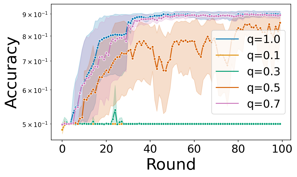
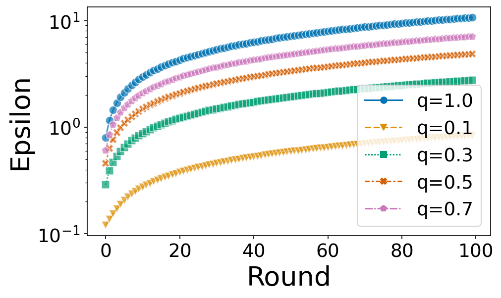
(a) Creditcard.

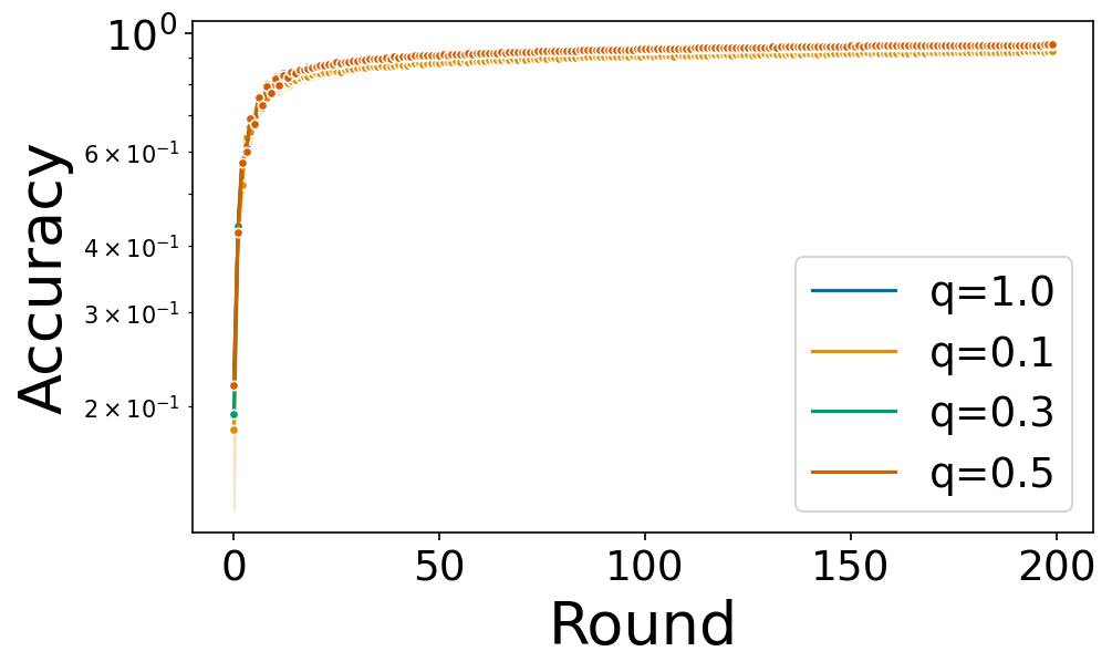
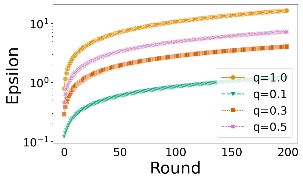
(b) MNIST.

Figure 10. User-level sub-sampling achieves a more competitive privacy-utility trade-off.

Effect of user-level sub-sampling. We evaluate the effect of user-level sub-sampling. Figure 10(b) illustrates how user-level sub-sampling affects the privacy-utility trade-offs on the Creditcard dataset with 1000 users. We report the test accuracy and ULDP privacy bounds for various sampling rates $q=0.1,0.3,0.5,0.7,1.0$. Basically, a tighter privacy bound is obtained at the expense of utility. As the results show, the degradation of utility due to sub-sampling could be acceptable to some extent (e.g., $q=0.7$) and there could be an optimal point for each setting. Figure 10(b) illustrates how user-level sub-sampling affects the privacy-utility trade-offs on MNIST with 10000 users, with sampling rates $q=0.1,0.3,0.5,1.0$. The results show that while privacy is greatly improved, there is less degradation in utility. This is due to the fact that there are a sufficient number of users, i.e., 10000. In the case of a larger user base, the effect of sub-sampling is greater and more important.

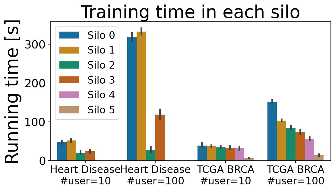
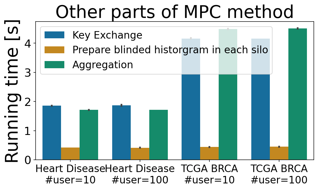
Figure 11. With a small model, the private weighting protocol has a practical execution time.

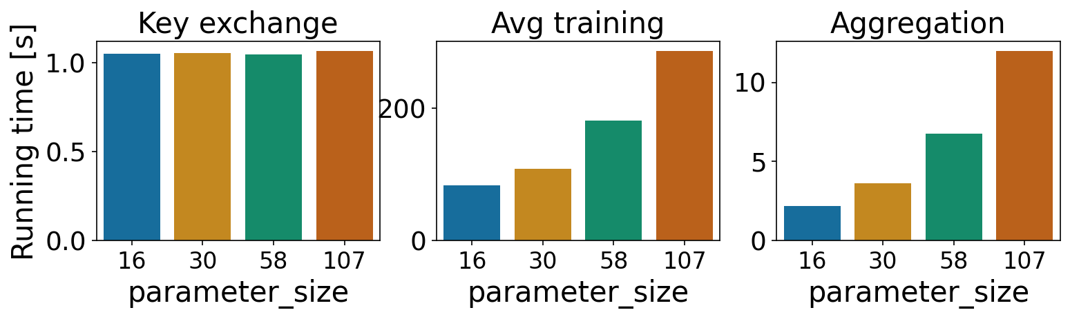
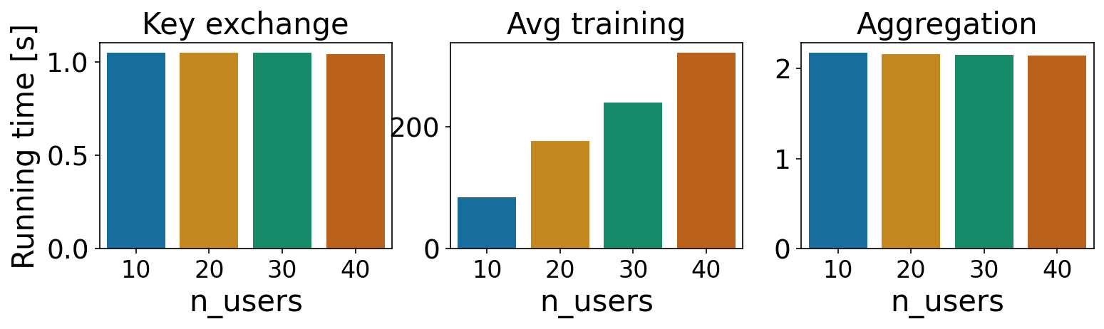
Figure 12. The dominant execution time grows linearly with parameter size (Top) and/or the number of users (Bottom).

Overhead of private weighting protocol. We evaluate the overheads of execution time with the private weighting protocol. Figure 11 shows the execution times following HeartDisease and TcgaBrca with the number of users 10 and 100, respectively, with a skewed (zipf) distribution. These two benchmark scenarios of cross-silo FL from (Ogier du Terrail et al., 2022) use small models. The left figure shows the time required for local training in each silo, and the right figure shows the execution time for key exchange, preparation of blinded histograms, and aggregation. As shown in the figure, the execution time of local training is dominant and it increases with a larger number of users. Overall, it shows realistic execution times under these benchmark scenarios (Ogier du Terrail et al., 2022).

Figure 12 shows the execution times of our proposed private weighting protocol (Protocol 4.1) with an artificial dataset with 10000 samples and a model with 16 parameters, 20 users, and 3 silos as default. These are on a considerably small scale. The major time-consuming parts of the protocol are key exchange, training in each silo, and aggregation on the server. The top three figures show the execution times on each part of the protocol with various parameter sizes from 16 to 107 and the bottom figures show the results on various number of users from 10 to 40. The execution time of local training is averaged by silos. The dominant part is the local training part, which is considered to be an overhead due to the computation with the Paillier encryption, which grows linearly with parameter size and/or the number of users. The larger parameter size increases the aggregation time on the server as well. Our implementation is based on the Python library (pyt, [n.d.]), which itself could be made faster by software implementation or hardware accelerators (Yang et al., 2020). However, it can be challenging to apply to larger models, such as DNNs, because the execution time increases linearly on a non-negligible scale with parameter size. Therefore, extending the proposed method to deep models with millions of parameters is a future challenge. It may be possible to replace such software-based encryption methods by using hardware-assisted Trusted Execution Environments, which have recently attracted attention in the FL field (Mo et al., 2021; Kato et al., 2023).

6. Conclusion

This study aimed to integrate user-level DP into FL, providing practical privacy guarantees for the trained model in general cross-silo scenarios. We proposed the first cross-silo ULDP FL framework where a user can have multiple records across silos. We designed an algorithm using per-user weighted clipping to directly satisfy ULDP instead of group-privacy. In addition, we developed an enhanced weighting strategy that improves the utility of our proposed method and a novel protocol that performs it privately. Finally, we demonstrated the effectiveness of the proposed method on several real-world datasets and showed that it performs significantly better than existing methods. We also verified that our proposed private protocol works in realistic time in existing cross-silo FL benchmark scenarios. For future work, research into the more scalable private protocols would be considered.

Appendix A Omitted Definition

Definition 0 (Sensitivity).

The sensitivity of a function $f$ for any two neighboring inputs $D,D^{\prime}\in\mathcal{D}$ is:

$$\Delta_{f}=\sup_{D,D^{\prime}\in\mathcal{D}}\|f(D)-f(D^{\prime})\|.$$

where $\lVert\cdot\rVert$ is a norm function defined in $f$’s output domain.

We consider $\ell 2$-norm ($\lVert\cdot\rVert_{2}$) as $\ell 2$-sensitivity due to adding a Gaussian noise.

Appendix B Omitted Figures

Here we illustrate the examples of record allocation described in Section 5.1. For Creditcard and MNIST, the number of silos $|S|$ is fixed at 5. We used 100, 1000 for Creditcard as $|U|$. For example, when $|U|=100$ and $|S|=5$, the record distribution of Creditcard dataset is shown in Figure 13. The number of records is plotted for each user and color-coded for each silo.

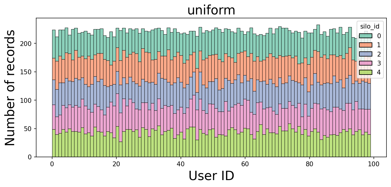
(a) uniform.

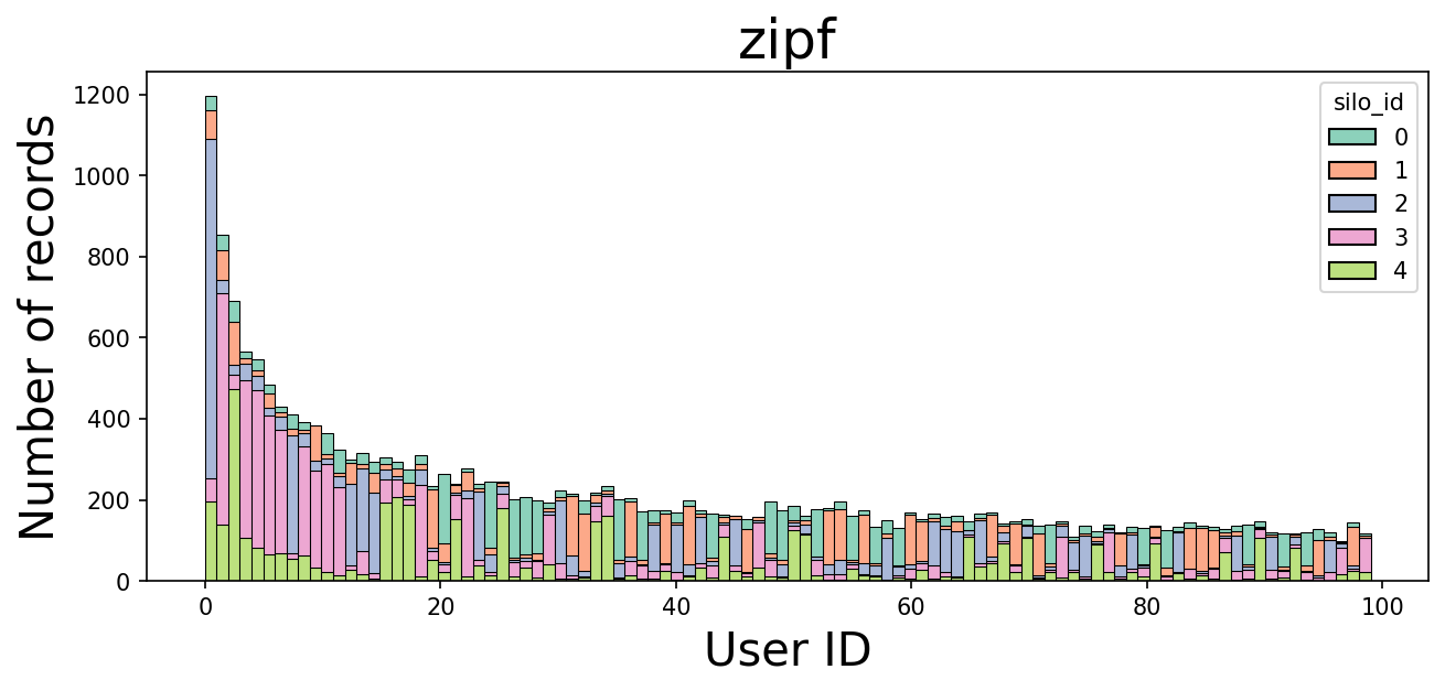
(b) zipf.

Figure 13. Example of record allocation on Creditcard.

Appendix C Proofs

C.1. Proof of Theorem 3

At each round $t$, due to the clipping operation (Line 14 in Algorithm 1), for each silo $s\in S$, any user’s contribution to $\Delta^{s}_{t}$ (Line 6) is limited to at most $C$ (regardless of the number of user records). Since a single user may exist in any silo, they contribute at most $|S|C$ to $\sum_{s\in S}{\Delta^{s}_{t}}$, which means the user-level sensitivity is $|S|C$. Therefore, when each silo adds Gaussian noise with variance $\sigma^{2}C^{2}|S|$, the aggregate $\sum_{s\in S}{\Delta^{s}_{t}}$ includes Gaussian noise with variance $\sigma^{2}C^{2}|S|^{2}$. Then, by Lemma 5, it satisfies $(\alpha,\frac{\alpha}{2\sigma^{2}})$-RDP for $\alpha>1$. And after $T$ rounds, it satisfies $(\alpha,\frac{T\alpha}{2\sigma^{2}})$-RDP by Lemma 3. Finally, by Lemma 4, we obtain the final result.

C.2. Proof of Theorem 4

In each silo $s\in S$, by performing DP-SGD with $Q$ epochs and $T$ rounds, we achieve record-level $(\alpha,\rho_{s}=\rho(\sigma,\gamma,QT))$-RDP. The actual value of $\rho_{s}$ is calculated numerically as described in (Mironov et al., 2019). RDP is known to satisfy parallel composition (Chaudhuri et al., 2019). That is, for disjoint databases $D_{1}$ and $D_{2}$, if $\mathcal{M}_{1}$ is $(\alpha,\rho_{1})$-RDP and $\mathcal{M}_{2}$ is $(\alpha,\rho_{2})$-RDP, their combined release $(\mathcal{M}_{1}(D_{1}),\mathcal{M}_{2}(D_{2}))$ satisfies $(\alpha,\mathrm{max}\{\rho_{1},\rho_{2}\})$-RDP. Since input databases $D_{s}$ for any silo $s\in S$ are disjoint from others, after $T$ rounds, the trained model satisfies $(\alpha,\rho=\max_{s\in S}\rho_{s})$-RDP for the entire cross-silo database $D=D_{1}\oplus...\oplus D_{|S|}$. Then, by applying Lemma 9 and Lemma 4, for any integer $k$ that is a power of 2 and any $\alpha\geq 2^{k+1}$, it also satisfies $(k,3^{k}\rho+\log{((\frac{\alpha}{2^{k}}-1)/\frac{\alpha}{2^{k}})}-(\log{\delta}+\log{\frac{\alpha}{2^{k}}})/(\frac{\alpha}{2^{k}}-1),\delta)$-GDP. By filtering with $\mathbf{B}$, we ensure that any user has at most $k$ records in $D$. The final result is obtained by Proposition 2. (An alternative method to compute $\epsilon$ is to use Lemma 8 instead of Lemma 9.)

C.3. Proof of Theorem 5

For any round $t$, due to the clipping operation (Line 16), for each silo $s\in S$ any user’s contribution to $\Delta^{s}_{t}$ (Line 6) is limited to at most $w_{s,u}C$ (regardless of the number of user records). Therefore, for $\sum_{s\in S}{\Delta^{s}_{t}}$ (Line 6), any user’s contribution is at most $\sum_{s\in S}w_{s,u}C=C$ since $\sum_{s\in S}{w_{s,u}}=1$. That means the user-level sensitivity is just $C$. Since each silo adds Gaussian noise with variance $\sigma^{2}C^{2}/|S|$, $\sum_{s\in S}{\Delta^{s}_{t}}$ includes Gaussian noise with variance $\sigma^{2}C^{2}$. Then, by Lemma 5, it satisfies $(\alpha,\frac{\alpha}{2\sigma^{2}})$-RDP for $\alpha>1$ in a user-level manner. And after $T$ rounds, it satisfies $(\alpha,\frac{T\alpha}{2\sigma^{2}})$-RDP by Lemma 3. Finally, by Lemma 4, we obtain the result.

C.4. Proof of Theorem 1

Initially, with regards to secure aggregation, the additive pair-wise masks cancel out as shown in (Bonawitz et al., 2017). For the difference, silo must participate in any rounds in our cross-silo FL. When collecting the histogram, additive masks are canceled out as follows:

$$B(N_{u})=\sum_{s\in S}{B(n_{s,u})}\quad+\sum_{s<s^{\prime}}{\underbrace{(r^{u}_{s,s^{\prime}}-r^{u}_{s^{\prime},s})}_{\text{canceled out}}}-\sum_{s>s^{\prime}}{\underbrace{(r^{u}_{s,s^{\prime}}-r^{u}_{s^{\prime},s})}_{\text{canceled out}}}$$

The same applies to secure aggregation for model delta. The mask is not directly added to the ciphertext (within the multiplication group of $n^{2}$); instead, scalar addition within $\mathbb{F}_{n}$ that takes advantage of the homomorphic property of the Paillier cryptosystem is utilized. As secure aggregation doesn’t result in any degradation of the aggregation outcome when all terms are within $\mathbb{F}_{n}$, our focus shifts to other components. Note that there are errors due to the handling of fixed-point numbers on a finite field. From the protocol description, $Enc_{\text{p}}(\Delta_{\text{sec}})$ is analyzed as follows:

$$Enc_{\text{p}}(\Delta_{\text{sec}}) =\sum_{s\in S}{Enc_{\text{p}}(\Delta^{s}_{t})}=\sum_{s\in S}{\sum_{u\in U}{Enc_{\text{p}}(\tilde{\Delta}^{s,u}_{t})}+z^{\prime}_{s}}$$

$$=\sum_{s\in S}{\sum_{u\in U}E^{s,u}_{t}n_{s,u}r_{u}C_{\text{LCM}}Enc_{\text{p}}(B_{\text{inv}}(N_{u}))+Z^{s}_{t}C_{\text{LCM}}}$$

$$\stackrel{{\scriptstyle(1)}}{{=}}Enc_{\text{p}}(\sum_{s\in S}{(\sum_{u\in U}{(E^{s,u}_{t}n_{s,u}r_{u}C_{\text{LCM}}B_{\text{inv}}(N_{u}))})+Z^{s}_{t}C_{\text{LCM}}})$$

$$=Enc_{\text{p}}(\sum_{s\in S}{(\sum_{u\in U}{(E^{s,u}_{t}n_{s,u}r_{u}C_{\text{LCM}}(r_{u}N_{u})^{-1}})+Z^{s}_{t}C_{\text{LCM}}}))$$

$$\stackrel{{\scriptstyle(2)}}{{=}}Enc_{\text{p}}(\sum_{s\in S}{(\sum_{u\in U}{(E^{s,u}_{t}n_{s,u}C_{-N_{u}}})+Z^{s}_{t}C_{\text{LCM}}}))$$

where $C_{-N_{u}}$ is the result of modular multiplication between $C_{\text{LCM}}$ and the modular multiplicative inverse of $N_{u}$, $E^{s,u}_{t}=\textsc{Encode}(\tilde{\Delta}^{s,u}_{t},P,n)$ and $Z^{s}_{t}=\textsc{Encode}(z^{s}_{t},P,n)$. Equation (1) is because all of $B_{\text{inv}}$, $E^{s,u}_{t}$, $n_{s,u}$, $r_{u}$ and $C_{\text{LCM}}$ $\in\mathbb{F}_{n}$. At (2), the modulo inverse of $r_{u}$ is canceled out because $r_{u}\in\mathbb{F}_{n}$ and $r_{u}$ almost always has a modulo inverse. However, this does not hold when $r_{u}$ and $n$ are not coprime. Let $p$ and $q$ be two large primes used in the Paillier cryptosystem, such that $n=pq$, then the probability of a random $r_{u}\in\mathbb{F}_{n}$ and $n$ are not coprime is

(5) $$\frac{n-1-\phi(n)}{n-1}=\frac{n-1-(p-1)(q-1)}{n-1},$$

where $\phi$ is Euler’s totient function. This probability is negligibly small when n is sufficiently large. In the case of user-level sub-sampling, $B_{\text{inv}}(N_{u})$ is set 0 and we see that only the model delta for user $u$ is all zeros, which produces exactly the same result as if the unselected users did not participate in the training round. The important condition is that if $N_{u}\leq N_{\text{max}}$ and $N_{u}$ is a factor of $C_{\text{LCM}}$, $C_{\text{LCM}}/N_{u}$ is always divisible on $\mathbb{Z}$ and the result is the same as on $\mathbb{F}_{n}$. Also if $\sum_{s\in S}{(\sum_{u\in U}{(E^{s,u}_{t}n_{s,u}C_{-N_{u}}})+Z^{s}_{t}C_{\text{LCM}}})\in\mathbb{Z}$ is smaller than $n$, it yields the same results on $\mathbb{Z}$ and $\mathbb{F}_{n}$. Hence, when these conditions are satisfied, decrypted value $\Delta_{\text{sec}}\in\mathbb{F}_{n}$ obtains the same result on $\Delta_{\text{sec}}\in\mathbb{Z}$. After decryption, we consider $\Delta_{\text{sec}}\in\mathbb{R}$. The final result is decoded by $\textsc{Decode}(\Delta_{\text{sec}},P,C_{\text{LCM}},n)\in\mathbb{R}$ as follows:

$$\textsc{Decode}(\Delta_{\text{sec}},P,C_{\text{LCM}},n)=\sum_{s\in S}{(\sum_{u\in U}{(\frac{n_{s,u}}{N_{u}}\tilde{\Delta}^{\prime}_{s,u,t})}+Z^{\prime}_{s,t}})$$

where $\tilde{\Delta}^{\prime}_{s,u,t}$ is the same as the result of computing $\tilde{\Delta}^{s,u}_{t}$ in fixed-point with precision $P$, and $Z^{\prime}_{s,t}$ is the same as $z^{s}_{t}$.

Therefore, the correctness of these calculations is satisfied when two conditions (1) $N_{u}\leq N_{\text{max}}$ and
(2) $\sum_{s\in S}{(\sum_{u\in U}{(E^{s,u}_{t}n_{s,u}C_{-N_{u}}})+Z^{s}_{t}C_{\text{LCM}}})<n$, are satisfied. To satisfy (1), $N_{\text{max}}$ must be sufficiently large, and a larger $N_{\text{max}}$ leads to a larger $C_{\text{LCM}}$. Hence, when we take $n$ is large, these conditions can be satisfied unless the parameters or noise take on unrealistically large values.

For example, suppose the range of the noise and aggregated model parameters is $[-10^{10},10^{10}]$, $P=10^{-10}$, $N_{\text{max}}=2000$ and $\lambda$ is 3072-bit security, we have $n>10^{924}$ by Paillier cryptosystem, $E^{s,u}_{t}<10^{20}$ , $Z^{s}_{t}<10^{20}$ and $C_{\text{LCM}}<10^{867}$. Then,
$\sum_{s\in S}{(\sum_{u\in U}{(E^{s,u}_{t}n_{s,u}C_{-N_{u}}})+Z^{s}_{t}C_{\text{LCM}}})<10^{888}<n$ and we satisfy the condition (2). $C_{\text{LCM}}$ grows exponentially with respect to $N_{\text{max}}$. One possible solution for this is that we can make it very small by limiting the number of records per user to several values. For example, $\{10^{1},10^{2},10^{3},10^{4}\}$ then $C_{\text{LCM}}=10^{4}$.

C.5. Proof of Theorem 2

Our approach relies on a private weighted sum aggregation technique employing the Paillier cryptosystem (Paillier, 1999; Liu et al., 2022) and secure aggregation (Bonawitz et al., 2017). Formal security arguments for these methodologies are available in their respective sources. The protocol is fully compatible with these works because all data exchanged is handled on $\mathbb{F}_{n}$ including random masks for secure aggregation.

A different view of the server from these basic methods is $B(N_{u})$ for all $u$, which is multiplicatively blinded aggregated histogram. Since $B(n_{s,u})$ for $s$ and $u$ is securely hidden by secure aggregation, only $B(N_{u})$ is the meaningful server view. $B(N_{u})$ is $r_{u}N_{u}\,(\text{mod}\,n)$ and this is randomly distributed on $\mathbb{F}_{n}$ if $r_{u}$ is uniformly distributed on $\mathbb{F}_{n}$. Also, the inverse of $B_{\text{inv}}(N_{u})$ is uniformly distributed as well. This is because the multiplication operation in a finite field is closed and bijective. Therefore, it is information-theoretically indistinguishable and private. Such multiplicative blinding has been also used in (Damgård et al., 2007). The view of the silos is the same as that in (Liu et al., 2022), even though the contents of the weights are sensitive, and privacy is protected by Paillier encryption. Note that the security of the initial DH key exchange and the security of the Paillier cryptosystem follow the security parameter $\lambda$, which is an input to the protocol.

C.6. Proof of Theorem 6

The many of techniques in the following proof are seen in (Yang et al., 2021; Zhang et al., 2022; Reddi et al., 2021).

For convenience, we define following quantities:

$$\alpha^{s,u}_{t} :=\cfrac{w_{s,u}C}{\max{(C,\eta_{l}\lVert\sum_{q\in[Q]}g^{s,u}_{t,q}\rVert)}},\;\tilde{\alpha}^{s,u}_{t}:=\cfrac{w_{s,u}C}{\max{(C,\eta_{l}\lVert\mathbb{E}\left[\sum_{q\in[Q]}g^{s,u}_{t,q}\right]\rVert)}},\;\bar{\alpha}_{t}:=\cfrac{1}{|S||U|}\sum_{s\in S}\sum_{u\in U}{\tilde{\alpha}^{s,u}_{t}},$$

(6) $$\Delta^{s,u}_{t} :=-\eta_{l}\sum_{q\in[Q]}{g^{s,u}_{t,q}}\cdot\alpha^{s,u}_{t},\;\tilde{\Delta}^{s,u}_{t}:=-\eta_{l}\sum_{q\in[Q]}{g^{s,u}_{t,q}}\cdot\tilde{\alpha}^{s,u}_{t},\;\bar{\Delta}^{s,u}_{t}:=-\eta_{l}\sum_{q\in[Q]}{g^{s,u}_{t,q}}\cdot\bar{\alpha}_{t},$$

(7) $$\breve{\Delta}^{s,u}_{t} :=-\eta_{l}\sum_{q\in[Q]}{\nabla f_{s,u}(x^{s,u}_{t,q})}\cdot\bar{\alpha}_{t},\;\Delta^{s}_{t}:=\sum_{u\in U}{\Delta^{s,u}_{t}},\;\tilde{\Delta}^{s}_{t}:=\sum_{u\in U}{\tilde{\Delta}^{s,u}_{t}},\;\bar{\Delta}^{s}_{t}:=\sum_{u\in U}{\bar{\Delta}^{s,u}_{t}},\;\breve{\Delta}^{s}_{t}:=\sum_{u\in U}{\breve{\Delta}^{s,u}_{t}}.$$

where expectation in $\tilde{\alpha}^{s,u}_{t}$ is taken over all possible randomness. Due to the smoothness in Assumption 1, we have

(8) $$f(x_{x+1})\leq f(x_{t})+\langle\nabla f(x_{t}),x_{t+1}-x_{t}\rangle+\frac{L}{2}\lVert x_{t+1}-x_{t}\rVert^{2}.$$

The model difference between two consecutive iterations can be represented as

(9) $$x_{x+1}-x_{t}=\eta_{g}\frac{1}{|S||U|}\sum_{s\in S}{(\Delta^{s}_{t}+z^{s}_{t})}$$

with random noise $z^{s}_{t}\sim\mathcal{N}(0,I\sigma^{2}C^{2}/|S|)$. Taking expectation of $f(x_{t+1})$ over the randomness at communication round $t$, we have:

$$\mathbb{E}\left[f(x_{x+1})\right] \leq f(x_{t})+\langle\nabla f(x_{t}),\mathbb{E}\left[x_{t+1}-x_{t}\right]\rangle+\frac{L}{2}\mathbb{E}\left[\lVert x_{t+1}-x_{t}\rVert^{2}\right]$$

$$=f(x_{t})+\eta_{g}\langle\nabla f(x_{t}),\mathbb{E}\left[\frac{1}{|S||U|}\sum_{s\in S}{(\Delta^{s}_{t}+z^{s}_{t})}\right]\rangle+\frac{L}{2}\eta_{g}^{2}\mathbb{E}\left[\left\lVert\frac{1}{|S||U|}\sum_{s\in S}{(\Delta^{s}_{t}+z^{s}_{t})}\right\rVert^{2}\right]$$

(10) $$=f(x_{t})+\eta_{g}\langle\nabla f(x_{t}),\mathbb{E}\left[\frac{1}{|S||U|}\sum_{s\in S}{\Delta^{s}_{t}}\right]\rangle+\frac{L}{2}\eta_{g}^{2}\mathbb{E}\left[\left\lVert\frac{1}{|S||U|}\sum_{s\in S}{\Delta^{s}_{t}}\right\rVert^{2}\right]+\frac{L}{2}\eta_{g}^{2}\frac{1}{|S|^{2}|U|^{2}}\sigma^{2}C^{2}d$$

where $d$ in the last expression is dimension of $x_{t}$ and in the last equation we use the fact that $z^{s}_{t}$ is zero mean normal distribution.

Firstly, we evaluate the first-order term of Eq. (C.6),

$$\langle\nabla f(x_{t}),\mathbb{E}\left[\frac{1}{|S||U|}\sum_{s\in S}{\Delta^{s}_{t}}\right]\rangle$$

(11) $$=\langle\nabla f(x_{t}),\mathbb{E}\left[\frac{1}{|S||U|}\sum_{s\in S}{(\Delta^{s}_{t}-\tilde{\Delta}^{s}_{t})}\right]\rangle+\langle\nabla f(x_{t}),\mathbb{E}\left[\frac{1}{|S||U|}\sum_{s\in S}{(\tilde{\Delta}^{s}_{t}-\bar{\Delta}^{s}_{t})}\right]\rangle+\langle\nabla f(x_{t}),\mathbb{E}\left[\frac{1}{|S||U|}\sum_{s\in S}{\bar{\Delta}^{s}_{t}}\right]\rangle,$$

and the last term of Eq. (C.6) can be evaluated as follows:

$$\langle\nabla f(x_{t}),\mathbb{E}\left[\frac{1}{|S||U|}\sum_{s\in S}{\bar{\Delta}^{s}_{t}}\right]\rangle$$

(12) $$=-\cfrac{\eta_{l}\bar{\alpha}_{t}Q}{2}\lVert\nabla f(x_{t})\rVert^{2}-\cfrac{\eta_{l}\bar{\alpha}_{t}}{2Q}\mathbb{E}\left[\left\lVert\cfrac{1}{\eta_{l}|S||U|\bar{\alpha}_{t}}\sum_{s\in S}{\breve{\Delta}^{s}_{t}}\right\rVert^{2}\right]+\cfrac{\eta_{l}\bar{\alpha}_{t}}{2}\mathbb{E}\left[\left\lVert\sqrt{Q}\nabla f(x_{t})+\cfrac{1}{\sqrt{Q}\eta_{l}|S||U|\bar{\alpha}_{t}}\sum_{s\in S}{\breve{\Delta}^{s}_{t}}\right\rVert^{2}\right].$$

This is because $\mathbb{E}\bar{\Delta}^{s}_{t}=\breve{\Delta}^{s}_{t}$ and $\langle a,b\rangle=-\frac{1}{2}\lVert a\rVert^{2}-\frac{1}{2}\lVert b\rVert^{2}+\frac{1}{2}\lVert a+b\rVert^{2}$ for any vector $a$, $b$.

We further upper bound the last term of Eq. C.6 as:

$$\mathbb{E}\left[\left\lVert\sqrt{Q}\nabla f(x_{t})+\cfrac{1}{\sqrt{Q}\eta_{l}|S||U|\bar{\alpha}_{t}}\sum_{s\in S}{\breve{\Delta}^{s}_{t}}\right\rVert^{2}\right] =Q\mathbb{E}\left[\left\lVert\nabla f(x_{t})+\cfrac{1}{Q\eta_{l}|S||U|\bar{\alpha}_{t}}\sum_{s\in S}{(\sum_{u\in U}{(-\eta_{l}\sum_{q\in[Q]}{\nabla f_{s,u}(x^{s,u}_{t,q})}\cdot\bar{\alpha}_{t}}))}\right\rVert^{2}\right]$$

$$=Q\mathbb{E}\left[\left\lVert\cfrac{1}{Q|S||U|}\sum_{s\in S}\sum_{u\in U}\sum_{q\in[Q]}{\nabla f_{s,u}(x_{t})-\nabla f_{s,u}(x^{s,u}_{t,q})}\right\rVert^{2}\right]$$

$$\stackrel{{\scriptstyle(a1)}}{{\leq}}Q\cdot\cfrac{1}{Q|S||U|}\mathbb{E}\left[\sum_{s\in S}\sum_{u\in U}\sum_{q\in[Q]}{\lVert\nabla f_{s,u}(x_{t})-\nabla f_{s,u}(x^{s,u}_{t,q})\rVert^{2}}\right]$$

$$\stackrel{{\scriptstyle(a2)}}{{\leq}}\cfrac{1}{|S||U|}\sum_{s\in S}\sum_{u\in U}\sum_{q\in[Q]}{L^{2}\mathbb{E}\left[{\lVert x_{t}-x^{s,u}_{t,q}\rVert^{2}}\right]}$$

(13) $$\stackrel{{\scriptstyle(a3)}}{{\leq}}L^{2}5Q^{2}\eta_{l}^{2}(\sigma_{l}^{2}+6Q\sigma_{g}^{2})+L^{2}30Q^{3}\eta_{l}^{2}\lVert\nabla f(x_{t})\rVert^{2},$$

where we use $\mathbb{E}\left[\lVert X_{1}+...+X_{n}\rVert^{2}\right]\leq n\mathbb{E}\left[\lVert X_{1}\rVert^{2}+...+\lVert X_{n}\rVert^{2}\right]$ at (a1), L-smoothness (Assumption 1) at (a2), and Lemma 3 of (Reddi et al., 2021) at (a3).

Secondly, we evaluate the second-order term in Eq. (C.6) as follows:

$$\mathbb{E} \left[\left\lVert\frac{1}{|S||U|}\sum_{s\in S}{\Delta^{s}_{t}}\right\rVert^{2}\right]$$

(14) $$\leq 3\mathbb{E}\left[\left\lVert\frac{1}{|S||U|}\sum_{s\in S}{\Delta^{s}_{t}-\tilde{\Delta}^{s}_{t}}\right\rVert^{2}\right]+3\mathbb{E}\left[\left\lVert\frac{1}{|S||U|}\sum_{s\in S}{\Delta^{s}_{t}-\bar{\Delta}^{s}_{t}}\right\rVert^{2}\right]+3\mathbb{E}\left[\left\lVert\frac{1}{|S||U|}\sum_{s\in S}{\bar{\Delta}^{s}_{t}}\right\rVert^{2}\right].$$

This is because $(a+b+c)^{2}\leq 3a^{2}+3b^{2}+3c^{2}$ holds when $a=A-B$, $b=B-C$, $c=C$ for all vector $A,B,C$. We can bound the expectation in the last term of Eq. (C.6) as follows:

$$\mathbb{E}\left[\left\lVert\frac{1}{|S||U|}\sum_{s\in S}{\bar{\Delta}^{s}_{t}}\right\rVert^{2}\right] =\mathbb{E}\left[\left\lVert\frac{1}{|S||U|}\sum_{s\in S}{\sum_{u\in U}{(\eta_{l}\sum_{q\in[Q]}{g^{s,u}_{t,q}}\cdot\bar{\alpha}_{t})}}\right\rVert^{2}\right]$$

$$\stackrel{{\scriptstyle(a4)}}{{=}}\eta_{l}^{2}\mathbb{E}\left[\left\lVert\frac{1}{|S||U|}\sum_{s\in S}{\sum_{u\in U}{\sum_{q\in[Q]}{\nabla f_{s,u}(x^{s,u}_{t,q})\cdot\bar{\alpha}_{t}}}}\right\rVert^{2}+\left\lVert\frac{1}{|S||U|}\sum_{s\in S}{\sum_{u\in U}{\sum_{q\in[Q]}{(\nabla f_{s,u}(x^{s,u}_{t,q})-g^{s,u}_{t,q})\cdot\bar{\alpha}_{t}}}}\right\rVert^{2}\right]$$

$$=\mathbb{E}\left[\left\lVert\frac{1}{|S||U|}\sum_{s\in S}{\breve{\Delta}^{s}_{t}}\right\rVert^{2}\right]+\cfrac{\eta_{l}^{2}\bar{\alpha}_{t}^{2}}{|S|^{2}|U|^{2}}\mathbb{E}\left[\left\lVert\sum_{s\in S}{\sum_{u\in U}{\sum_{q\in[Q]}{(\nabla f_{s,u}(x^{s,u}_{t,q})-g^{s,u}_{t,q})}}}\right\rVert^{2}\right]$$

$$\stackrel{{\scriptstyle(a5)}}{{\leq}}\mathbb{E}\left[\left\lVert\frac{1}{|S||U|}\sum_{s\in S}{\breve{\Delta}^{s}_{t}}\right\rVert^{2}\right]+\cfrac{\eta_{l}^{2}\bar{\alpha}_{t}^{2}}{|S|^{2}|U|^{2}}\mathbb{E}\left[\sum_{s\in S}{\sum_{u\in U}{\sum_{q\in[Q]}{\left\lVert\nabla f_{s,u}(x^{s,u}_{t,q})-g^{s,u}_{t,q}\right\rVert^{2}}}}\right]$$

$$\leq\mathbb{E}\left[\left\lVert\frac{1}{|S||U|}\sum_{s\in S}{\breve{\Delta}^{s}_{t}}\right\rVert^{2}\right]+\cfrac{\eta_{l}^{2}\bar{\alpha}_{t}^{2}}{|S|^{2}|U|^{2}}\sum_{s\in S}{\sum_{u\in U}{\sum_{q\in[Q]}{\sigma_{l}^{2}}}}$$

(15) $$\leq\mathbb{E}\left[\left\lVert\frac{1}{|S||U|}\sum_{s\in S}{\breve{\Delta}^{s}_{t}}\right\rVert^{2}\right]+\cfrac{\eta_{l}^{2}\bar{\alpha}_{t}^{2}}{|S||U|}Q\sigma_{l}^{2},$$

where we use $\mathbb{E}\left[\lVert X\rVert^{2}\right]=\mathbb{E}\left[\lVert X-\mathbb{E}\left[X\right]\rVert^{2}\right]+\lVert\mathbb{E}\left[X\right]\rVert^{2}$ at (a4), and $\mathbb{E}\left[\lVert X_{1}+...+X_{n}\rVert^{2}\right]\leq\mathbb{E}\left[\lVert X_{1}\rVert^{2}+...+\lVert X_{n}\rVert^{2}\right]$ when $\forall i,j,i\not=j$, $X_{i}$ and $X_{j}$ are independent and $\mathbb{E}\left[X_{i}\right]=0$ and Assumption 2 at (a5).

Lastly, combining all of above, we have

$$\mathbb{E}\left[f(x_{x+1})\right] \leq f(x_{t})+\eta_{g}\langle\nabla f(x_{t}),\mathbb{E}\left[\frac{1}{|S||U|}\sum_{s\in S}{(\Delta^{s}_{t}-\tilde{\Delta}^{s}_{t})}\right]\rangle+\eta_{g}\langle\nabla f(x_{t}),\mathbb{E}\left[\frac{1}{|S||U|}\sum_{s\in S}{(\tilde{\Delta}^{s}_{t}-\bar{\Delta}^{s}_{t})}\right]\rangle$$

$$\;\;\;\;-\frac{1}{2}\eta_{g}\eta_{l}\bar{\alpha}_{t}Q\lVert\nabla f(x_{t})\rVert^{2}-\frac{1}{2}\cfrac{\eta_{g}}{Q|S|^{2}|U|^{2}\eta_{l}\bar{\alpha}_{t}}\mathbb{E}\left[\left\lVert\sum_{s\in S}{\breve{\Delta}^{s}_{t}}\right\rVert^{2}\right]$$

$$\;\;\;\;+\cfrac{\eta_{g}\eta_{l}\bar{\alpha}_{t}}{2}\left(L^{2}5Q^{2}\eta_{l}^{2}(\sigma_{l}^{2}+6Q\sigma_{g}^{2})+L^{2}30Q^{3}\eta_{l}^{2}\lVert\nabla f(x_{t})\rVert^{2}\right)$$

$$\;\;\;\;+\frac{3}{2}L\eta_{g}^{2}\mathbb{E}\left[\left\lVert\frac{1}{|S||U|}\sum_{s\in S}{\Delta^{s}_{t}-\tilde{\Delta}^{s}_{t}}\right\rVert^{2}\right]+\frac{3}{2}L\eta_{g}^{2}\mathbb{E}\left[\left\lVert\frac{1}{|S||U|}\sum_{s\in S}{\tilde{\Delta}^{s}_{t}-\bar{\Delta}^{s}_{t}}\right\rVert^{2}\right]+\frac{3}{2}L\eta_{g}^{2}\frac{1}{|S|^{2}|U|^{2}}\mathbb{E}\left[\left\lVert\sum_{s\in S}{\breve{\Delta}^{s}_{t}}\right\rVert^{2}\right]$$

$$\;\;\;\;+\frac{3}{2}\cfrac{\eta_{g}^{2}\eta_{l}^{2}\bar{\alpha}_{t}^{2}LQ\sigma_{l}^{2}}{|S||U|}+\frac{1}{2}\cfrac{L\eta_{g}^{2}\sigma^{2}C^{2}d}{|S|^{2}|U|^{2}}$$

$$=f(x_{t})-\left(\frac{1}{2}\eta_{l}\eta_{g}\bar{\alpha}_{t}Q-\cfrac{\eta_{g}\eta_{l}\bar{\alpha}_{t}}{2}L^{2}30Q^{3}\eta_{l}^{2}\right)\lVert\nabla f(x_{t})\rVert^{2}$$

$$\;\;\;\;-\left(\frac{1}{2}\cfrac{\eta_{g}}{Q|S|^{2}|U|^{2}\eta_{l}\bar{\alpha}_{t}}-\frac{3}{2}L\eta_{g}^{2}\frac{1}{|S|^{2}|U|^{2}}\right)\mathbb{E}\left[\left\lVert\sum_{s\in S}{\breve{\Delta}^{s}_{t}}\right\rVert^{2}\right]$$

$$\;\;\;\;+\cfrac{\eta_{g}\eta_{l}\bar{\alpha}_{t}}{2}L^{2}5Q^{2}\eta_{l}^{2}(\sigma_{l}^{2}+6Q\sigma_{g}^{2})+\frac{3}{2}\cfrac{\eta_{g}^{2}\eta_{l}^{2}\bar{\alpha}_{t}^{2}LQ\sigma_{l}^{2}}{|S||U|}+\frac{1}{2}\cfrac{L\eta_{g}^{2}\sigma^{2}C^{2}d}{|S|^{2}|U|^{2}}$$

$$\;\;\;\;+\underbrace{\eta_{g}\langle\nabla f(x_{t}),\mathbb{E}\left[\frac{1}{|S||U|}\sum_{s\in S}{(\Delta^{s}_{t}-\tilde{\Delta}^{s}_{t})}\right]\rangle+\eta_{g}\langle\nabla f(x_{t}),\mathbb{E}\left[\frac{1}{|S||U|}\sum_{s\in S}{(\tilde{\Delta}^{s}_{t}-\bar{\Delta}^{s}_{t})}\right]\rangle}_{A_{1}}$$

$$\;\;\;\;+\underbrace{\frac{3}{2}L\eta_{g}^{2}\mathbb{E}\left[\left\lVert\frac{1}{|S||U|}\sum_{s\in S}{\Delta^{s}_{t}-\tilde{\Delta}^{s}_{t}}\right\rVert^{2}\right]+\frac{3}{2}L\eta_{g}^{2}\mathbb{E}\left[\left\lVert\frac{1}{|S||U|}\sum_{s\in S}{\tilde{\Delta}^{s}_{t}-\bar{\Delta}^{s}_{t}}\right\rVert^{2}\right]}_{A_{2}}$$

$$\stackrel{{\scriptstyle(a6)}}{{\leq}}f(x_{t})-\eta_{l}\eta_{g}\bar{\alpha}_{t}Q\left(\frac{1}{2}-15L^{2}Q^{2}\eta_{l}^{2}\right)\lVert\nabla f(x_{t})\rVert^{2}$$

$$\;\;\;\;+\cfrac{\eta_{g}\eta_{l}\bar{\alpha}_{t}}{2}L^{2}5Q^{2}\eta_{l}^{2}(\sigma_{l}^{2}+6Q\sigma_{g}^{2})+\frac{3}{2}\cfrac{\eta_{g}^{2}\eta_{l}^{2}\bar{\alpha}_{t}^{2}LQ\sigma_{l}^{2}}{|S||U|}+\frac{1}{2}\cfrac{L\eta_{g}^{2}\sigma^{2}C^{2}d}{|S|^{2}|U|^{2}}+A_{1}+A_{2}$$

(16) $$\stackrel{{\scriptstyle(a7)}}{{\leq}}f(x_{t})-c\eta_{l}\eta_{g}\bar{\alpha}_{t}Q\lVert\nabla f(x_{t})\rVert^{2}+\cfrac{\eta_{g}\eta_{l}\bar{\alpha}_{t}}{2}L^{2}5Q^{2}\eta_{l}^{2}(\sigma_{l}^{2}+6Q\sigma_{g}^{2})+\frac{3}{2}\cfrac{\eta_{g}^{2}\eta_{l}^{2}\bar{\alpha}_{t}^{2}LQ\sigma_{l}^{2}}{|S||U|}+\frac{1}{2}\cfrac{L\eta_{g}^{2}\sigma^{2}C^{2}d}{|S|^{2}|U|^{2}}+A_{1}+A_{2}$$

where (a6) follows from $\left(\frac{1}{2}\frac{\eta_{g}}{Q|S|^{2}|U|^{2}\eta_{l}\bar{\alpha}_{t}}-\frac{3}{2}L\eta_{g}^{2}\frac{1}{|S|^{2}|U|^{2}}\right)\geq 0$ if $\eta_{g}\eta_{l}\leq\frac{1}{3QL\bar{\alpha}_{t}}$ and replacing the last terms with $A_{1}$ and $A_{2}$, and (a7) holds because there exists a constant $c>0$ satisfying $\left(\frac{1}{2}-15L^{2}Q^{2}\eta_{l}^{2}\right)>c>0$ if $\eta_{l}<\frac{1}{\sqrt{30}QL}$. Divide both sides of (C.6) by $c\eta_{l}\eta_{g}Q\bar{\alpha}_{t}$, sum over $t$ from $0$ to $T-1$, divide both sides by $T$, and rearrange, we have

$$\cfrac{1}{T}\sum_{t=0}^{T-1}{\mathbb{E}\left[\left\lVert\nabla f(x_{t})\right\rVert^{2}\right]}\leq\; \cfrac{1}{cT\eta_{g}\eta_{l}Q}\left(\mathbb{E}\left[\frac{f(x_{0})}{\bar{\alpha}_{0}}\right]-\mathbb{E}\left[\frac{f(x_{T})}{\bar{\alpha}_{T-1}}\right]\right)$$

$$\;\;\;+\frac{5}{2c}L^{2}Q\eta_{l}^{2}(\sigma_{l}^{2}+6Q\sigma_{g}^{2})+\cfrac{3L\eta_{g}\eta_{l}\sigma_{l}^{2}}{2c|S||U|}\cfrac{1}{T}\sum_{t=0}^{T-1}{\bar{\alpha}_{t}}+\cfrac{L\eta_{g}\sigma^{2}C^{2}d}{2c\eta_{l}Q|S|^{2}|U|^{2}}\cfrac{1}{T}\sum_{t=0}^{T-1}{\frac{1}{\bar{\alpha}_{t}}}$$

$$\;\;\;+\underbrace{\cfrac{1}{c\eta_{l}Q}\cfrac{1}{T}\sum_{t=0}^{T-1}{\frac{1}{\bar{\alpha}_{t}}}{\mathbb{E}\left[\langle\nabla f(x_{t}),\mathbb{E}\left[\frac{1}{|S||U|}\sum_{s\in S}{(\Delta^{s}_{t}-\tilde{\Delta}^{s}_{t})}\right]\rangle+\langle\nabla f(x_{t}),\mathbb{E}\left[\frac{1}{|S||U|}\sum_{s\in S}{(\tilde{\Delta}^{s}_{t}-\bar{\Delta}^{s}_{t})}\right]\rangle\right]}}_{B_{1}}$$

(17) $$\;\;\;+\underbrace{\cfrac{3L\eta_{g}}{2c\eta_{l}Q}\cfrac{1}{T}\sum_{t=0}^{T-1}{\frac{1}{\bar{\alpha}_{t}}}{\left(\mathbb{E}\left[\left\lVert\frac{1}{|S||U|}\sum_{s\in S}{\Delta^{s}_{t}-\tilde{\Delta}^{s}_{t}}\right\rVert^{2}\right]+\mathbb{E}\left[\left\lVert\frac{1}{|S||U|}\sum_{s\in S}{\tilde{\Delta}^{s}_{t}-\bar{\Delta}^{s}_{t}}\right\rVert^{2}\right]\right)}}_{B_{2}}.$$

Let $\smash{\displaystyle\max_{s\in S,u\in U,t\in[T]}}{\left(\frac{C}{\max{(C,\eta_{l}\lVert\mathbb{E}\left[\sum_{q\in[Q]}g^{s,u}_{t,q}\right]\rVert)}}\right)}$ be $\bar{C}$, and $\smash{\displaystyle\min_{s\in S,u\in U,t\in[T]}}{\left(\frac{C}{\max{(C,\eta_{l}\lVert\mathbb{E}\left[\sum_{q\in[Q]}g^{s,u}_{t,q}\right]\rVert)}}\right)}$ be $\underline{C}$, $\frac{1}{|S|}\underline{C}\leq\bar{\alpha}_{t}\leq\frac{1}{|S|}\bar{C}$ since $\bar{\alpha}_{t}$’s definition and $\frac{1}{|S|}\sum_{s\in S}w_{s,u}=\frac{1}{|S|}$. Using this, (C.6) is evaluated as follows:

$$\cfrac{1}{T}\sum_{t=0}^{T-1}{\mathbb{E}\left[\left\lVert\nabla f(x_{t})\right\rVert^{2}\right]}\leq\; \cfrac{1}{cT\eta_{g}\eta_{l}Q|S|}\left(\mathbb{E}\left[\frac{f(x_{0})}{\underline{C}}\right]-\mathbb{E}\left[\frac{f(x_{T})}{\bar{C}}\right]\right)$$

$$\;\;\;+\frac{5}{2c}L^{2}Q\eta_{l}^{2}(\sigma_{l}^{2}+6Q\sigma_{g}^{2})+\cfrac{3\bar{C}L\eta_{g}\eta_{l}\sigma_{l}^{2}}{2c|S|^{2}|U|}+\cfrac{L\eta_{g}\sigma^{2}C^{2}d}{2c\underline{C}\eta_{l}Q|S||U|^{2}}$$

$$\;\;\;+\underbrace{\cfrac{|S|}{c\underline{C}\eta_{l}Q}\cfrac{1}{T}\sum_{t=0}^{T-1}{\mathbb{E}\left[\langle\nabla f(x_{t}),\mathbb{E}\left[\frac{1}{|S||U|}\sum_{s\in S}{(\Delta^{s}_{t}-\tilde{\Delta}^{s}_{t})}\right]\rangle+\langle\nabla f(x_{t}),\mathbb{E}\left[\frac{1}{|S||U|}\sum_{s\in S}{(\tilde{\Delta}^{s}_{t}-\bar{\Delta}^{s}_{t})}\right]\rangle\right]}}_{B_{1}}$$

(18) $$\;\;\;+\underbrace{\cfrac{3L\eta_{g}|S|}{2c\underline{C}\eta_{l}Q}\cfrac{1}{T}\sum_{t=0}^{T-1}{\left(\mathbb{E}\left[\left\lVert\frac{1}{|S||U|}\sum_{s\in S}{\Delta^{s}_{t}-\tilde{\Delta}^{s}_{t}}\right\rVert^{2}\right]+\mathbb{E}\left[\left\lVert\frac{1}{|S||U|}\sum_{s\in S}{\tilde{\Delta}^{s}_{t}-\bar{\Delta}^{s}_{t}}\right\rVert^{2}\right]\right)}}_{B_{2}}.$$

$B_{1}$ and $B_{2}$ is upper-bounded as follows:

$$B_{1} \leq\cfrac{|S|}{c\underline{C}\eta_{l}Q}\cfrac{1}{T}\sum_{t=0}^{T-1}{\mathbb{E}\left[\langle\nabla f(x_{t}),\mathbb{E}\left[\frac{1}{|S||U|}\sum_{s\in S}\sum_{u\in U}{\left|\Delta^{s,u}_{t}-\tilde{\Delta}^{s,u}_{t}\right|}\right]\rangle+\langle\nabla f(x_{t}),\mathbb{E}\left[\frac{1}{|S||U|}\sum_{s\in S}\sum_{u\in U}{\left|\tilde{\Delta}^{s,u}_{t}-\bar{\Delta}^{s,u}_{t}\right|}\right]\rangle\right]}$$

$$\leq\cfrac{G^{2}}{c\underline{C}|U|}\cfrac{1}{T}\sum_{t=0}^{T-1}{\mathbb{E}\left[\sum_{s\in S}\sum_{u\in U}{\left(\left|\alpha^{s,u}_{t}-\tilde{\alpha}^{s,u}_{t}\right|+\left|\tilde{\alpha}^{s,u}_{t}-\bar{\alpha}_{t}\right|\right)}\right]},$$

$$B_{2} \stackrel{{\scriptstyle(a8)}}{{\leq}}\cfrac{3L\eta_{g}|S|}{2c\underline{C}\eta_{l}Q}\cfrac{1}{T}\sum_{t=0}^{T-1}{\left(\mathbb{E}\left[\frac{1}{|S||U|}\sum_{s\in S}\sum_{u\in U}\left|{\Delta^{s,u}_{t}-\tilde{\Delta}^{s,u}_{t}}\right|^{2}\right]+\mathbb{E}\left[\frac{1}{|S||U|}\sum_{s\in S}\sum_{u\in U}\left|{\tilde{\Delta}^{s,u}_{t}-\bar{\Delta}^{s,u}_{t}}\right|^{2}\right]\right)}$$

(19) $$\leq\cfrac{3L\eta_{g}\eta_{l}QG^{2}}{2c\underline{C}|U|}\cfrac{1}{T}\sum_{t=0}^{T-1}{\mathbb{E}\left[\sum_{s\in S}\sum_{u\in U}{\left(\left|\alpha^{s,u}_{t}-\tilde{\alpha}^{s,u}_{t}\right|^{2}+\left|\tilde{\alpha}^{s,u}_{t}-\bar{\alpha}_{t}\right|^{2}\right)}\right]}$$

with

$$\left|\Delta^{s,u}_{t}-\tilde{\Delta}^{s,u}_{t}\right| \leq\eta_{l}QG\left|\alpha^{s,u}_{t}-\tilde{\alpha}^{s,u}_{t}\right|,$$

(20) $$\left|\tilde{\Delta}^{s,u}_{t}-\bar{\Delta}^{s,u}_{t}\right| \leq\eta_{l}QG\left|\tilde{\alpha}^{s,u}_{t}-\bar{\alpha}_{t}\right|,$$

by Assumption 3 of globally bounded gradients, and we use the same technique at (a8) as (a1).

References

• (1)
• pyt ([n.d.]) [n.d.]. Python Paillier. https://github.com/data61/python-paillier.
• Abadi et al. (2016) Martin Abadi, Andy Chu, Ian Goodfellow, H Brendan McMahan, Ilya Mironov, Kunal Talwar, and Li Zhang. 2016. Deep learning with differential privacy. In Proceedings of the 2016 ACM SIGSAC conference on computer and communications security. 308–318.
• Agarwal et al. (2021) Naman Agarwal, Peter Kairouz, and Ziyu Liu. 2021. The skellam mechanism for differentially private federated learning. Advances in Neural Information Processing Systems 34 (2021), 5052–5064.
• Alexandru and Pappas (2022) Andreea B. Alexandru and George J. Pappas. 2022. Private Weighted Sum Aggregation. IEEE Transactions on Control of Network Systems 9, 1 (2022), 219–230. https://doi.org/10.1109/TCNS.2021.3094788
• Amin et al. (2019) Kareem Amin, Alex Kulesza, Andres Munoz, and Sergei Vassilvtiskii. 2019. Bounding user contributions: A bias-variance trade-off in differential privacy. In International Conference on Machine Learning. PMLR, 263–271.
• Balle et al. (2020) Borja Balle, Gilles Barthe, Marco Gaboardi, Justin Hsu, and Tetsuya Sato. 2020. Hypothesis testing interpretations and renyi differential privacy. In International Conference on Artificial Intelligence and Statistics. PMLR, 2496–2506.
• Bell et al. (2020) James Henry Bell, Kallista A Bonawitz, Adrià Gascón, Tancrède Lepoint, and Mariana Raykova. 2020. Secure single-server aggregation with (poly) logarithmic overhead. In Proceedings of the 2020 ACM SIGSAC Conference on Computer and Communications Security. 1253–1269.
• Bonawitz et al. (2017) Keith Bonawitz, Vladimir Ivanov, Ben Kreuter, Antonio Marcedone, H Brendan McMahan, Sarvar Patel, Daniel Ramage, Aaron Segal, and Karn Seth. 2017. Practical secure aggregation for privacy-preserving machine learning. In proceedings of the 2017 ACM SIGSAC Conference on Computer and Communications Security. 1175–1191.
• Chaudhuri et al. (2019) Kamalika Chaudhuri, Jacob Imola, and Ashwin Machanavajjhala. 2019. Capacity Bounded Differential Privacy. Curran Associates Inc., Red Hook, NY, USA.
• Cheu et al. (2019) Albert Cheu, Adam Smith, Jonathan Ullman, David Zeber, and Maxim Zhilyaev. 2019. Distributed differential privacy via shuffling. In Advances in Cryptology–EUROCRYPT 2019: 38th Annual International Conference on the Theory and Applications of Cryptographic Techniques, Darmstadt, Germany, May 19–23, 2019, Proceedings, Part I 38. Springer, 375–403.
• Damgård et al. (2007) Ivan Damgård, Martin Geisler, and Mikkel Krøigaard. 2007. Efficient and secure comparison for on-line auctions. In Information Security and Privacy: 12th Australasian Conference, ACISP 2007, Townsville, Australia, July 2-4, 2007. Proceedings 12. Springer, 416–430.
• Dwork (2006) Cynthia Dwork. 2006. Differential privacy. In Proceedings of the 33rd international conference on Automata, Languages and Programming-Volume Part II. Springer-Verlag, 1–12.
• Dwork et al. (2014) Cynthia Dwork, Aaron Roth, et al. 2014. The algorithmic foundations of differential privacy. Foundations and Trends® in Theoretical Computer Science 9, 3–4 (2014), 211–407.
• Epasto et al. (2020) Alessandro Epasto, Mohammad Mahdian, Jieming Mao, Vahab Mirrokni, and Lijie Ren. 2020. Smoothly bounding user contributions in differential privacy. Advances in Neural Information Processing Systems 33 (2020), 13999–14010.
• Erlingsson et al. (2020) Úlfar Erlingsson, Vitaly Feldman, Ilya Mironov, Ananth Raghunathan, Shuang Song, Kunal Talwar, and Abhradeep Thakurta. 2020. Encode, shuffle, analyze privacy revisited: Formalizations and empirical evaluation. arXiv preprint arXiv:2001.03618 (2020).
• Geyer et al. (2017) Robin C Geyer, Tassilo Klein, and Moin Nabi. 2017. Differentially private federated learning: A client level perspective. NIPS 2017 Workshop: Machine Learning on the Phone and other Consumer Devices (2017).
• Girgis et al. (2021) Antonious Girgis, Deepesh Data, Suhas Diggavi, Peter Kairouz, and Ananda Theertha Suresh. 2021. Shuffled model of differential privacy in federated learning. In International Conference on Artificial Intelligence and Statistics. PMLR, 2521–2529.
• Goddard (2017) Michelle Goddard. 2017. The EU General Data Protection Regulation (GDPR): European regulation that has a global impact. International Journal of Market Research 59, 6 (2017), 703–705.
• Kaggle (2018) Kaggle. 2018. Credit Card Fraud Detection dataset. https://www.kaggle.com/datasets/mlg-ulb/creditcardfraud. Accessed: 2023-08-03.
• Kairouz et al. (2021) Peter Kairouz, Ziyu Liu, and Thomas Steinke. 2021. The distributed discrete gaussian mechanism for federated learning with secure aggregation. In International Conference on Machine Learning. PMLR, 5201–5212.
• Kamath (2020) Gautam Kamath. 2020. CS 860 : Algorithms for Private Data Analysis Fall 2020 Lecture 5 — Approximate Differential Privacy. http://www.gautamkamath.com/CS860notes/lec5.pdf. [Online; accessed 23-June-2023].
• Kato et al. (2021) Fumiyuki Kato, Yang Cao, and Masatoshi Yoshikawa. 2021. Preventing manipulation attack in local differential privacy using verifiable randomization mechanism. In Data and Applications Security and Privacy XXXV: 35th Annual IFIP WG 11.3 Conference, DBSec 2021, Calgary, Canada, July 19–20, 2021, Proceedings 35. Springer, 43–60.
• Kato et al. (2023) Fumiyuki Kato, Yang Cao, and Masatoshi Yoshikawa. 2023. Olive: Oblivious Federated Learning on Trusted Execution Environment against the Risk of Sparsification. Proc. VLDB Endow. 16, 10 (aug 2023), 2404–2417. https://doi.org/10.14778/3603581.3603583
• Levy et al. (2021) Daniel Levy, Ziteng Sun, Kareem Amin, Satyen Kale, Alex Kulesza, Mehryar Mohri, and Ananda Theertha Suresh. 2021. Learning with user-level privacy. Advances in Neural Information Processing Systems 34 (2021), 12466–12479.
• Liew et al. (2022) Seng Pei Liew, Tsubasa Takahashi, Shun Takagi, Fumiyuki Kato, Yang Cao, and Masatoshi Yoshikawa. 2022. Network shuffling: Privacy amplification via random walks. In Proceedings of the 2022 International Conference on Management of Data. 773–787.
• Liu et al. (2022) Ken Liu, Shengyuan Hu, Steven Z Wu, and Virginia Smith. 2022. On privacy and personalization in cross-silo federated learning. Advances in Neural Information Processing Systems 35 (2022), 5925–5940.
• Liu et al. (2020) Yuhan Liu, Ananda Theertha Suresh, Felix Xinnan X Yu, Sanjiv Kumar, and Michael Riley. 2020. Learning discrete distributions: user vs item-level privacy. Advances in Neural Information Processing Systems 33 (2020), 20965–20976.
• Lowy et al. (2023) Andrew Lowy, Ali Ghafelebashi, and Meisam Razaviyayn. 2023. Private non-convex federated learning without a trusted server. In International Conference on Artificial Intelligence and Statistics. PMLR, 5749–5786.
• Lowy and Razaviyayn (2023) Andrew Lowy and Meisam Razaviyayn. 2023. Private Federated Learning Without a Trusted Server: Optimal Algorithms for Convex Losses. In The Eleventh International Conference on Learning Representations. https://openreview.net/forum?id=TVY6GoURrw
• McMahan et al. (2018) H Brendan McMahan, Galen Andrew, Ulfar Erlingsson, Steve Chien, Ilya Mironov, Nicolas Papernot, and Peter Kairouz. 2018. A general approach to adding differential privacy to iterative training procedures. arXiv preprint arXiv:1812.06210 (2018).
• McMahan et al. (2016) H Brendan McMahan, Eider Moore, Daniel Ramage, and Blaise Agüera y Arcas. 2016. Federated learning of deep networks using model averaging. arXiv preprint arXiv:1602.05629 (2016).
• McMahan et al. (2017) H Brendan McMahan, Daniel Ramage, Kunal Talwar, and Li Zhang. 2017. Learning differentially private recurrent language models. arXiv preprint arXiv:1710.06963 (2017).
• McSherry (2009) Frank D McSherry. 2009. Privacy integrated queries: an extensible platform for privacy-preserving data analysis. In Proceedings of the 2009 ACM SIGMOD International Conference on Management of data. 19–30.
• Mironov (2017) Ilya Mironov. 2017. Rényi differential privacy. In 2017 IEEE 30th computer security foundations symposium (CSF). IEEE, 263–275.
• Mironov et al. (2019) Ilya Mironov, Kunal Talwar, and Li Zhang. 2019. R$\backslash$’enyi differential privacy of the sampled gaussian mechanism. arXiv preprint arXiv:1908.10530 (2019).
• Mo et al. (2021) Fan Mo, Hamed Haddadi, Kleomenis Katevas, Eduard Marin, Diego Perino, and Nicolas Kourtellis. 2021. PPFL: privacy-preserving federated learning with trusted execution environments. In Proceedings of the 19th annual international conference on mobile systems, applications, and services. 94–108.
• Nasr et al. (2019) Milad Nasr, Reza Shokri, and Amir Houmansadr. 2019. Comprehensive privacy analysis of deep learning: Passive and active white-box inference attacks against centralized and federated learning. In 2019 IEEE symposium on security and privacy (SP). IEEE, 739–753.
• Ogier du Terrail et al. (2022) Jean Ogier du Terrail, Samy-Safwan Ayed, Edwige Cyffers, Felix Grimberg, Chaoyang He, Regis Loeb, Paul Mangold, Tanguy Marchand, Othmane Marfoq, Erum Mushtaq, Boris Muzellec, Constantin Philippenko, Santiago Silva, Maria Teleńczuk, Shadi Albarqouni, Salman Avestimehr, Aurélien Bellet, Aymeric Dieuleveut, Martin Jaggi, Sai Praneeth Karimireddy, Marco Lorenzi, Giovanni Neglia, Marc Tommasi, and Mathieu Andreux. 2022. FLamby: Datasets and Benchmarks for Cross-Silo Federated Learning in Realistic Healthcare Settings. In Advances in Neural Information Processing Systems, S. Koyejo, S. Mohamed, A. Agarwal, D. Belgrave, K. Cho, and A. Oh (Eds.), Vol. 35. Curran Associates, Inc., 5315–5334.
• Paillier (1999) Pascal Paillier. 1999. Public-key cryptosystems based on composite degree residuosity classes. In International conference on the theory and applications of cryptographic techniques. Springer, 223–238.
• Paulik et al. (2021) Matthias Paulik, Matt Seigel, Henry Mason, Dominic Telaar, Joris Kluivers, Rogier van Dalen, Chi Wai Lau, Luke Carlson, Filip Granqvist, Chris Vandevelde, et al. 2021. Federated Evaluation and Tuning for On-Device Personalization: System Design & Applications. arXiv preprint arXiv:2102.08503 (2021).
• Ramaswamy et al. (2019) Swaroop Ramaswamy, Rajiv Mathews, Kanishka Rao, and Françoise Beaufays. 2019. Federated learning for emoji prediction in a mobile keyboard. arXiv preprint arXiv:1906.04329 (2019).
• Reddi et al. (2021) Sashank Reddi, Zachary Burr Charles, Manzil Zaheer, Zachary Garrett, Keith Rush, Jakub Konečný, Sanjiv Kumar, and Brendan McMahan (Eds.). 2021. Adaptive Federated Optimization. https://openreview.net/forum?id=LkFG3lB13U5
• So et al. (2023) Jinhyun So, Ramy E Ali, Başak Güler, Jiantao Jiao, and A Salman Avestimehr. 2023. Securing secure aggregation: Mitigating multi-round privacy leakage in federated learning. In Proceedings of the AAAI Conference on Artificial Intelligence, Vol. 37. 9864–9873.
• Takagi et al. (2023) Shun Takagi, Fumiyuki Kato, Yang Cao, and Masatoshi Yoshikawa. 2023. From Bounded to Unbounded: Privacy Amplification via Shuffling with Dummies. In 2023 IEEE 36th Computer Security Foundations Symposium (CSF). IEEE, 457–472.
• Vatsalan et al. (2017) Dinusha Vatsalan, Ziad Sehili, Peter Christen, and Erhard Rahm. 2017. Privacy-preserving record linkage for big data: Current approaches and research challenges. Handbook of big data technologies (2017), 851–895.
• Wang et al. (2019) Yu-Xiang Wang, Borja Balle, and Shiva Prasad Kasiviswanathan. 2019. Subsampled rényi differential privacy and analytical moments accountant. In The 22nd International Conference on Artificial Intelligence and Statistics. PMLR, 1226–1235.
• Wilson et al. (2020) Royce J Wilson, Celia Yuxin Zhang, William Lam, Damien Desfontaines, Daniel Simmons-Marengo, and Bryant Gipson. 2020. Differentially private SQL with bounded user contribution. Proceedings on privacy enhancing technologies 2020, 2 (2020), 230–250.
• Yang et al. (2021) Haibo Yang, Minghong Fang, and Jia Liu. 2021. Achieving Linear Speedup with Partial Worker Participation in Non-IID Federated Learning. Proceedings of ICLR (2021).
• Yang et al. (2020) Zhaoxiong Yang, Shuihai Hu, and Kai Chen. 2020. FPGA-based hardware accelerator of homomorphic encryption for efficient federated learning. arXiv preprint arXiv:2007.10560 (2020).
• Zhang et al. (2022) Xinwei Zhang, Xiangyi Chen, Mingyi Hong, Zhiwei Steven Wu, and Jinfeng Yi. 2022. Understanding clipping for federated learning: Convergence and client-level differential privacy. In International Conference on Machine Learning, ICML 2022.
• Zhao et al. (2020) Bo Zhao, Konda Reddy Mopuri, and Hakan Bilen. 2020. idlg: Improved deep leakage from gradients. arXiv preprint arXiv:2001.02610 (2020).