Novel regular black holes: geometry, source and shadow

Abstract

We propose a two-parameter, static and spherically symmetric regular geometry, which, for specific parameter values represents a regular black hole. The matter required to support such spacetimes within the framework of General Relativity (GR), is found to violate the energy conditions, though not in the entire domain of the radial coordinate. A particular choice of the parameters reduces the regular black hole to a singular, mutated Reissner–Nordström geometry. It also turns out that our regular black hole is geodesically complete. Fortunately, despite energy condition violation, we are able to construct a viable source, within the framework of GR coupled to matter, for our regular geometry. The source term involves a nonlinear magnetic monopole in a chosen version of nonlinear electrodynamics. Finally, we obtain the shadow profile of the regular black hole and try to estimate the metric parameters using some recent observational results from the EHT collaboration.

I Introduction

In recent years, the detection of gravitational waves from binary black hole mergers, black hole–neutron star binaries as well as neutron star-neutron star binaries Ligo1 ; Ligo2 ; Ligo3 ; Ligo4 have boosted research in gravitational physics. On another front, imaging observations on shadows due to the strong gravitational lensing around black holes in different galaxies, have provided useful information about such supermassive compact objects Akiyama1 ; Akiyama2 ; Akiyama3 ; Akiyama4 ; Akiyama5 ; Akiyama6 ; Akiyama7 ; Akiyama8 ; Akiyama9 ; Akiyama10 ; Akiyama11 ; Akiyama12 . Since Einstein’s theory of General Relativity (GR) is, by and large, the most acceptable theory of gravity today, the known rotating vacuum solution of Einstein’s equation, i.e. the Kerr solution, along with its properties, must explain phenomena related to such compact objects having horizons. It is, by now known, that imaging observations have more or less confirmed that the compact objects have a Kerr-like behaviour within a small uncertainty. However, to describe such compact objects, other solutions with horizons, predicted by different theories of gravity cannot be completely ignored. This implies a sort of ‘degeneracy’ in the sense that ‘many models’ can explain available data successfully. Breaking the ‘degeneracy’ will therefore require more observations as well as newer theoretical models.

On the other hand, from a theoretical perspective, the Hawking-Penrose singularity theorems Hawking with certain assumptions (energy conditions among them) have indeed proved that black hole solutions in GR possess a spacetime singularity(geodesic incompleteness). This is normally projected as a sign of inconsistency of classical GR and one would like to get rid of or avoid such singularities in some way, classical or quantum. However, one does not quite have a universally accepted resolution of this ‘singularity problem’.

Thus, from an observational perspective (as mentioned above) as well as the desire for well-behaved solutions in a theory of gravity, one is motivated to search for non-singular (regular) solutions in GR as well as in modified gravity theories.

Regular black holes are known potential candidates for such non-singular solutions. They may violate the Strong Energy Condition (SEC) and, therefore, can circumvent the singularity theorem Ansoldi ; Zaslavskii . As classical GR fails at the singularity, Sakharov Sakharov and Gliner Gliner , invoking quantum aspects, indicated that a de Sitter core could replace the singularity inside the horizon. Based on this idea, in 1968, Bardeen first proposed a static spherically symmetric regular black hole spacetime Bardeen . Since then, numerous proposals for regular black holes Bardeen2 ; Bardeen3 ; Hayward ; Roman ; Dymnikova ; Dymnikova1 ; Ayon1 ; Ayon3 ; Frolov ; Frolov2 ; Frolov3 ; Balart ; Bronnikov ; simpson ; Carballo2 ; Carballo3 ; Bambi ; Ghosh ; Sajadi ; Roy ; tapo1 have come up. The first proposal for the matter source of a regular black hole of the Bardeen type was made using a nonlinear electric or magnetic monopole Ayon1 ; Ayon2 ; Ayon3 ; Ayon4 ; Ayon5 i.e., a nonlinear electromagnetic field Lagrangian $(\mathcal{L}(\mathbf{F}))$ coupled with gravity was found to be capable of generating the matter required to support such a spacetime. Since then, several regular black hole models have emerged wherein a nonlinear electromagnetic field Lagrangian is employed as a matter source Balart ; Fan ; Zhong ; Bronnikov3 ; Bronnikov4 ; somalic .

Though popular of late, there are several criticisms of a regular black hole. First, we still do not understand properly the nature and dynamics of the source Lagrangian $(\mathcal{L}(\mathbf{F}))$. In other words, we have much to learn about the so-called nonlinear Maxwell-like equations. Second, each of the constructed regular black hole models have a different source Lagrangian $(\mathcal{L}(\mathbf{F}))$, which means we do not have a single, well-defined Lagrangian which can take on different functional forms when solutions for the input fields $(\mathbf{F})$ are used to describe the required matter for regular black holes. In addition, the mass inflation instability Poisson1 ; Poisson2 also appears to be a serious issue. The mass function increases exponentially under a perturbation at the inner horizon. Recently, significant efforts have been put forward to resolve the problem Bonanno ; Carballo , but the issue remains open.

Despite the shortcomings related to any research on regular black holes, we prefer to be hopeful and look for directions and approaches that might potentially provide novel insights about their properties. Let us now state our proposal to build novel spacetimes representing regular black holes. Our work is motivated by the Einstein-Rosen bridge construction Rosen , where the line element may be specified as;

$$ds^{2}=-\Big{(}1-\frac{b_{0}^{2}}{r^{2}}\Big{)}dt^{2}+\frac{dr^{2}}{1-\frac{b_{0}^{2}}{r^{2}}}+r^{2}(d\theta^{2}+\sin^{2}{\theta}d\phi^{2})$$ (1)

We choose the above singular line element and regularise the metric functions such that all curvature components and scalars become regular everywhere. Though our proposed regular black hole does violate the classical energy conditions in some domain of the radial coordinate, it is different in its geometric structure from other known regular black holes, all of which reduce to the Schwarzschild black hole for a zero value of the regularizing parameter. In a sense, we are able to show that it is not always necessary to ‘regularise around Schwarzschild’. Further, the process of regularisation about a solution built out of energy-condition violating matter may lead to a situation where regularisation not only remedies the singular character but also improves the status of the energy conditions vis-a-vis their satisfaction/violation. The ensuing sections of this article provide examples addressing these points.

Our article is organised as follows. In Section II, we propose our line element and provide a detailed study of its geometry, the energy conditions and check its non-singular character. In Section III, we construct the source for the geometry using nonlinear electrodynamics. Section IV discusses the shadow of the regular black hole and checks its viability with reference to observational data. Finally, in Section V, we conclude with some future directions.

II The proposed geometry and its features

As stated in the Introduction, we propose a non-singular, two-parameter, static and spherically symmetric spacetime which may represent a regular black hole. Developing on the idea briefly outlined above, we write down a line element of the following form:

$$ds^{2}=-\Big{(}1-\frac{b_{0}^{2}r^{2}}{(r^{2}+g^{2})^{2}}\Big{)}dt^{2}+\Big{(}1-\frac{b_{0}^{2}r^{2}}{(r^{2}+g^{2})^{2}}\Big{)}^{-1}dr^{2}+r^{2}\Big{(}d\theta^{2}+\sin^{2}\theta d\phi^{2}\Big{)}.$$ (2)

Here, $g^{2}$ is the regularizing parameter and the choice of the metric functions is largely inspired by earlier constructions due to Bardeen Bardeen . Note that our metric is not similar or related to the well-known regular black hole spacetimes of Bardeen, Hayward, or Simpson-Visser Bardeen ; Hayward ; simpson , all of which reduce to the standard Schwarzschild line element when the regularizing parameter vanishes. Instead, corresponding to the parameter value $g^{2}=0$, our metric becomes a mutated, singular Reissner–Nordström (RN) solution with an imaginary charge and a vanishing mass parameter. Further, the spacetime metric is asymptotically Minkowski, i.e.

$$g_{tt}\to\ -1\hskip 19.91684ptand\hskip 19.91684ptg_{rr}\to\ 1\hskip 19.91684ptas\hskip 19.91684ptr\to\ \infty$$

For small values of $r$, the metric behaves like de-Sitter space, i.e.

$$g_{tt}\to\ -(1-c_{1}^{2}r^{2})\hskip 19.91684ptand\hskip 19.91684ptg^{rr}\to\ 1-c_{1}^{2}r^{2}\hskip 19.91684ptas\hskip 19.91684ptr\to\ 0$$

Before proceeding further, let us mention the natural domain of the coordinates:

$$r\in(0,\infty);\hskip 25.6073ptt\in(-\infty,\infty);\hskip 25.6073pt\theta\in[0,\pi];\hskip 25.6073pt\phi\in(0,2\pi]$$

One can write the above metric in terms of the following reparameterization $g^{2}=m^{2}b_{0}^{2}$, where $m^{2}$ is a dimensionless quantity. Such a parameterization helps in calculations. The line element, with this choice, becomes:

$$ds^{2}=-\Big{(}1-\frac{b_{0}^{2}r^{2}}{(r^{2}+m^{2}b_{0}^{2})^{2}}\Big{)}dt^{2}+\Big{(}1-\frac{b_{0}^{2}r^{2}}{(r^{2}+m^{2}b_{0}^{2})^{2}}\Big{)}^{-1}dr^{2}+r^{2}\Big{(}d\theta^{2}+\sin^{2}\theta d\phi^{2}\Big{)}$$ (3)

The roots of the equation $g_{tt}=0$ are null hypersurfaces and represent the horizons of our black hole. Below, we discuss the nature of the spacetime and location of the horizons based on the various ranges of parameter values of $m^{2}$.

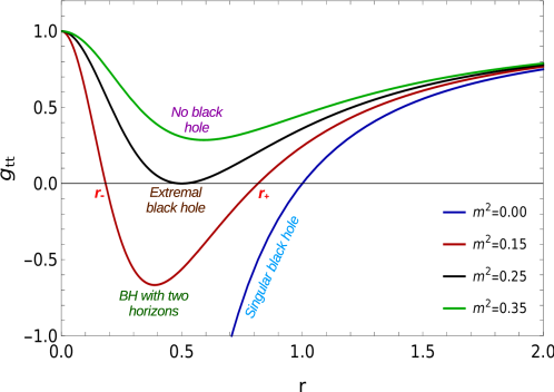
Figure 1: Plot of the redshift function with $r$ for different values of $m^{2}$

• If $m^{2}=0$, the geometry is a singular, $M=0$ RN type solution with $g_{tt}=g^{rr}=1-\frac{b_{0}^{2}}{r^{2}}$ having a horizon at $r=b_{0}$. It is not a regular solution. Note that the term involving the ‘charge’ has a sign opposite to that for standard RN spacetime.

• If $0<m^{2}\leq 0.25$, the geometry represents a family of regular black holes. $g_{tt}=0$ has four roots, two positive and two negative. As $r\in(0,\infty)$, we consider only positive roots as horizon locations. Hence we have a black hole spacetime with two horizons. In this specified range of $m^{2}$, inner horizon$(r_{-})$ and outer horizon$(r_{+})$ vary between $0<r_{-}\leq 0.5b_{0}$ and $b_{0}>r_{+}\geq 0.5b_{0}$ respectively. At $m^{2}=0.25$, inner and outer horizons coalesce into a single horizon. This is the analog of the extremal limit, for which $b_{0}^{2}=4g^{2}$. Figure 1 depicts how change in $m^{2}$ leads to variation in the number of horizons in our spacetime.

• If $m^{2}>0.25$, there are no real roots of the equation $g_{tt}=0$, i.e. we have a regular spacetime without a singularity or a horizon.

Hence we may conclude that we have a family of regular black holes with two horizons when $0<m^{2}<0.25$. The solution has an extremal limit similar to RN. One may try to understand this extremal limit a little better. The original line element, in the extremal limit takes the form:

$$ds^{2}=-\Big{(}1-\frac{4g^{2}r^{2}}{(r^{2}+g^{2})^{2}}\Big{)}dt^{2}+\Big{(}1-\frac{4g^{2}r^{2}}{(r^{2}+g^{2})^{2}}\Big{)}^{-1}dr^{2}+r^{2}\Big{(}d\theta^{2}+\sin^{2}\theta d\phi^{2}\Big{)}.$$ (4)

The geometry is very similar to that of the extremal RN black hole. If we embed a two-dimensional $t=const$, $\theta=\frac{\pi}{2}$ slice in Euclidean space (cylindrical coordinates), the profile function $z(r)$ takes the form:

$$z(r)=\pm g\ln\left(\left(\frac{r}{g}\right)^{2}-1\right)$$ (5)

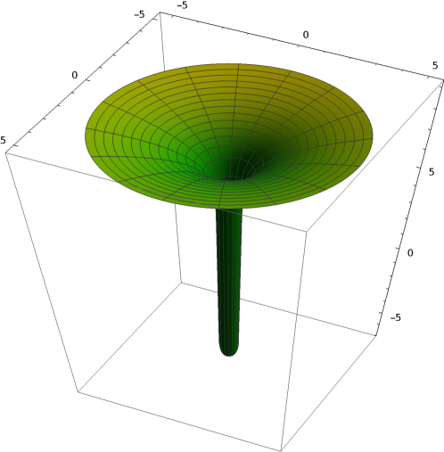
Figure 2: Embedding diagram of the extremal rbh metric shows a horn-like profile

which diverges to negative (positive) infinity at $r=g$ for the plus (minus) signs, respectively. The profile is like a horn or a trumpet and is similar in structure to that for the extremal RN spacetime.

Next, we study the regularity of curvature tensors and scalars as proof of the regularity of the spacetime. We also examine geodesic completeness in our geometry and check the energy conditions (assuming General Relativity as the theory of gravity).

II.1 Curvature tensors and invariants

To investigate the singular/regular nature of our geometry, one may look for the finiteness of the Riemann and Ricci tensor components in the entire domain of coordinates. Tensor components will, of course, be frame dependent. However, individual components and their finiteness usually indicate regularity. The non-zero Riemann curvature components in the frame basis are:

$$R^{01}{}_{10} =-\frac{(g^{4}-8g^{2}r^{2}+3r^{4})b_{0}^{2}}{(r^{2}+g^{2})^{4}}$$ (6)

$$R^{02}{}_{20} =R^{03}{}_{30}=R^{21}{}_{12}=R^{31}{}_{13}=\frac{(r^{2}-g^{2})b_{0}^{2}}{(r^{2}+g^{2})^{3}}$$

$$R^{32}{}_{23} =-\frac{b_{0}^{2}}{(r^{2}+g^{2})^{2}}$$

Assuming $g^{2}\neq 0$, the Riemann tensor components have a finite limit: $-\frac{b_{0}^{2}}{g^{4}}$ at $r\to\ 0$. Again, for $r\to\ \infty$, all components tend to $0$, ensuring the asymptotically flat nature of the spacetime.
The non-zero Ricci tensor components in the frame basis are:

$$R_{00}= -R_{11}=-\frac{(3g^{4}-8g^{2}r^{2}+r^{4})b_{0}^{2}}{(r^{2}+g^{2})^{4}}$$ (7)

$$R_{22}= R_{33}=\frac{(3g^{2}-r^{2})b_{0}^{2}}{(r^{2}+g^{2})^{3}}$$

The components of the Ricci tensor also reach a finite value at $r\to\ 0$ and vanish as $r\to\ \infty$. We can, therefore, partially conclude that there is no singularity in the metric, and it represents a family of regular black holes.

The more important quantities to analyse are the scalar curvature invariants Dymnikova ; Ayon1 . In 4D spacetime, one can construct fourteen independent curvature invariants from the Riemann curvature tensor components Weinberg . However, given the symmetries of our spacetime, finiteness of the three invariants – namely, the Ricci scalar, the Ricci contraction and the Kretschmann scalar – confirms the finiteness of all other invariants Hu . Therefore, we only examine these three invariants.
The Ricci scalar is given as:

$$R=g^{\mu\nu}R_{\mu\nu}=\frac{12b_{0}^{2}(g^{4}-g^{2}r^{2})}{(r^{2}+g^{2})^{2}}$$ (8)

The Ricci contraction turns out to be,

$$R_{\mu\nu}R^{\mu\nu}=\frac{4b_{0}^{4}(9g^{8}-18g^{6}r^{2}+34g^{4}r^{4}-10g^{2}r^{6}+r^{8})}{(r^{2}+g^{2})^{8}}$$ (9)

And the Kretschmann scalar is:

$$K=R_{\mu\nu\lambda\delta}R^{\mu\nu\lambda\delta}=\frac{8b_{0}^{4}(3g^{8}-6g^{6}r^{2}+34g^{4}r^{4}-22g^{2}r^{6}+7r^{8})}{(r^{2}+g^{2})^{8}}$$ (10)

As $r\to\ 0$, all the curvature scalars reach a finite value and tend to zero at $r\to\ \infty$, which confirms the non-singular nature of the above geometry.

II.2 Geodesic completeness

Regularity of curvature tensors and curvature invariants are required but inadequate for testing the singular nature of a spacetime. According to Wald ; Hawking ; Modesto ; Carballo4 ; Carballo5 ; tapo2 , the completeness of all causal geodesics is a necessary prerequisite for a regular spacetime. In this section, we look at the null and timelike geodesics in our geometry to analyze geodesic completeness. Let us start with radial timelike geodesics, which satisfy the following equation,

$$g_{tt}\dot{t}^{2}+g_{rr}\dot{r}^{2}=-1$$ (11)

where the dot represents the derivative with respect to affine parameter$(\lambda)$. Since the line element is static, we have a timelike Killing vector with the corresponding conserved quantity as $E=-g_{tt}\dot{t}$. Using this, the equation for radial timelike geodesics becomes,

$$\dot{r}^{2}=E^{2}-1+\frac{b_{0}^{2}r^{2}}{(r^{2}+g^{2})^{2}}$$ (12)

The affine parameter can be defined in the following way,

$$\lambda(r)=\int\frac{dr}{\sqrt{\dot{r}^{2}}}$$ (13)

This may be integrated using eq.(12) to determine how $\lambda$ varies as a function of $r$. For small values of $r$, our metric acts like de-Sitter space, and if $r=0$ is a regular point, the affine parameter is finite from any arbitrary point to $r=0$. As a result, the coordinate system may be hypothetically extended beyond $r=0$, i.e. towards negative $r$ values. Again, such an expansion is possible because a coordinate system is not a physical quantity. There are two alternatives for negative values of $r$: (i) one can locate a pole of $\dot{r}^{2}$, say at $r=-l$, where $\dot{r}^{2}$ diverges and if the affine parameter to reach the point is finite, then one cannot extend the co-ordinate beyond $r=-l$ (similar to $r=0$ in the Schwarzschild case), (ii) $\dot{r}^{2}$ is positive or negative and continuous up to $r\to\ -\infty$ which means for appropriate values of $E^{2}$, the trajectories of massive particles can be extended to negative values of $r$ up to $-\infty$. Thus, any divergence of $\dot{r}^{2}$ would indicate geodesic breakdown. Hence, to check geodesic completeness, our job is to check if there are any singularities in negative values of $r$ or it is regular up to $r\to\ -\infty$ with an infinite value of the affine parameter.
To perform this exercise, we have followed the prescription mentioned in Modesto . First, one can define the effective radial potential $(V_{eff}=E^{2}-\dot{r}^{2})$ in terms of the parametrization mentioned earlier. We have

$$V_{eff}(r)=1-\frac{b_{0}^{2}r^{2}}{(r^{2}+m^{2}b_{0}^{2})^{2}}$$ (14)

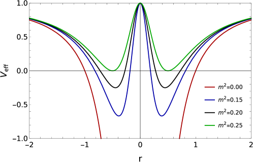
Figure 3: Plot of effective potential as function of $r$ for different values of $m^{2}$

In Figure 3, we plot the effective potential for the extended domain of $r$, i.e. $(-\infty,\infty)$. We have a continuous effective potential for $0<m^{2}\leq 0.25$. A massive particle with enough energy can travel up to $r\to-\infty$. On the other hand, the singular solution ($m^{2}=0$), exhibits a discontinuity in the effective potential at $r=0$. As a result, in this case, the massive particle will approach $r=0$ within a finite affine parameter, indicating the presence of a singularity. Figure 4 shows the behaviour of the kinetic energy of massive particles. We notice a continuity in the behaviour of kinetic energy for $0<m^{2}\leq 0.25$, (Figure 4 (left)). However, the kinetic energy is negative if $E^{2}<1$. When $E^{2}=1$, kinetic energy reaches zero at $r=0$, and massive particles need a large affine parameter to get there. However, if $E^{2}>1$ a massive particle will reach $r=0$ in a finite affine parameter before moving away to $r\to-\infty$. Figure 4 (right) illustrates the kinetic energy behaviour of massive particles in the singular geometry ($m^{2}=0$). It demonstrates that the kinetic energy diverges at $r=0$, regardless of the value of the total energy. As a result, within a finite affine parameter, a massive particle will reach $r=0$, where the geodesic will terminate.

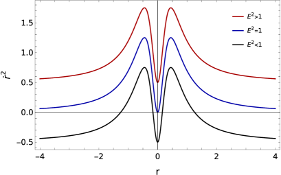
Figure 4: (Left) plot of the $\dot{r}^{2}$ with $r$ of the regular metric ($m^{2}=0.20$) for different $E^{2}$. (Right) variation of $\dot{r}^{2}$ of the singular metric ($m^{2}=0$) shows a divergence at $r=0$.

Next, the same procedure is followed for null geodesics. The right-hand side of eq.(11) is now zero. Here too, there is no pathology in the effective potential or kinetic term, and null geodesics can be extended to $r\to-\infty$. However, a termination of geodesics is evident in the singular metric $(m^{2}=0)$ for massless particles too.

To represent the causal structure of our regular spacetime, we extend the coordinates maximally Ramon . In Figure 5. $r_{+}$, $r_{-}$ are the outer and inner horizons, respectively. The interval from the outer horizon ($r_{+}$) to asymptotic infinity ($r\to\infty$) is encoded in the region I. Region II lies between the outer and inner horizons. Unlike the singular RN type metric $(m^{2}=0)$, the core of the regular spacetime $(0<m^{2}\leq 0.25)$ is a de-Sitter space. Region III, therefore, depicts the range from the inner horizon ($r_{-}$) to $r=0$. Region IV represents an asymptotic flat space through the regular core at $r=0$ to $r\to-\infty$. In conclusion, our regular black hole geometry is geodesically complete for both massive and massless particles. However, the singular RN-type metric is geodesically incomplete.

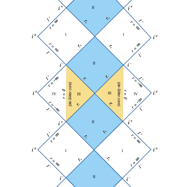
Figure 5: Plot of maximal extension of our regular metric $(0<m^{2}\leq 0.25)$ showing its geodesic completeness.

II.3 Energy momentum tensors and energy conditions

Regular black holes can avoid the Penrose singularity theorem by violating the strong energy condition Ansoldi ; Zaslavskii . Therefore, analyses of the energy conditions are important to study regular spacetime Bambi2 ; Lan . In this section, we have studied different energy conditions, namely the null energy condition (NEC), the weak energy condition (WEC), the dominant energy condition (DEC) and the strong energy condition (SEC). We write the diagonal elements of the required stress-energy tensor, in the frame basis, using the Einstein field equations $G_{ab}=\kappa T_{ab}$. This gives us the following expressions for the components of $T_{ab}$:

$$\rho=-\tau=\frac{(3g^{2}-r^{2})b_{0}^{2}}{\kappa(r^{2}+g^{2})^{3}}=-\frac{b_{0}^{2}r^{2}}{\kappa(r^{2}+g^{2})^{3}}+3g^{2}\frac{b_{0}^{2}}{\kappa(r^{2}+g^{2})^{3}}$$ (15)

$$p=-\frac{(3g^{4}-8g^{2}r^{2}+r^{4})b_{0}^{2}}{\kappa(r^{2}+g^{2})^{4}}=-\frac{r^{2}(r^{2}-2g^{2})b_{0}^{2}}{\kappa(r^{2}+g^{2})^{4}}-3g^{2}\frac{(g^{2}-2r^{2})b_{0}^{2}}{\kappa(r^{2}+g^{2})^{4}}$$ (16)

Notice that the decomposition indicated in the extreme right of Eqns (15) and (16) show the parts of $\rho$, $\tau$ and $p$ which are energy condition violating (first term) and energy condition satisfying (second term). Also the second terms in the split shown are exclusively dependent on the regularisation parameter $g$ and reduce to zero when $g=0$.

Let us now analyze different classical energy conditions as mentioned above and see whether the ‘matter required’ to support this spacetime violates/satisfies them.

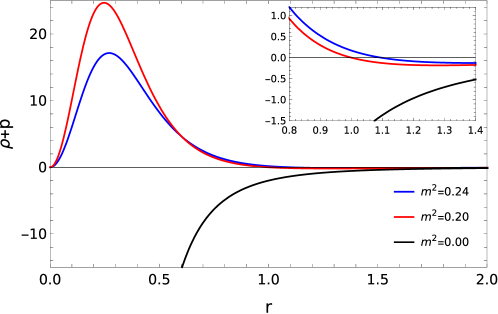
Figure 6: Plot of $\rho+p$ with $r$ for different values of $m^{2}$. Blue and red lines represent $\rho+p$ having $m^{2}$ value in the range $0<m^{2}\leq 0.25$. The black curve is for the singular metric

$\bullet$ Null Energy Condition : For all values of $r$, $g^{2}$, and $b_{0}^{2}$, $\rho+p\geq 0$ and $\rho+\tau\geq 0$ must be met in order to satisfy the null energy condition. The first of the criteria in the NEC is met here since, according to equation (15), $\rho+\tau=0$. For the second, we have;

$$\rho+p =\frac{(3g^{2}-r^{2})b_{0}^{2}}{\kappa(r^{2}+g^{2})^{3}}-\frac{(3g^{4}-8g^{2}r^{2}+r^{4})b_{0}^{2}}{\kappa(r^{2}+g^{2})^{4}}$$ (17)

$$=\frac{2(r^{2}/b_{0}^{2})(5m^{2}-(r^{2}/b_{0}^{2}))}{\kappa b_{0}^{2}((r^{2}/b_{0}^{2})+m^{2})^{4}}$$

It is clear from the equation above that for all allowed values of $m^{2}$, $\rho+p\geq 0$ in the range of $r^{2}\leq 5m^{2}b_{0}^{2}$. As a result, we know exactly what range of $r$ the NEC is fulfilled in. We show how the value of $\rho+p$ varies with $r$ in Figure 6. It should be noted that for the singular RN metric $(m^{2}=0)$ $\rho+p\leq 0$ over the whole domain of $r$. Thus, the regularisation of the singular RN metric$(m^{2}=0)$ does provide a range of $r$ where the NEC is fulfilled.

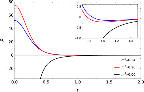
Figure 7: Plot of $\rho$ with $r$ for different values of $m^{2}$. Blue and red lines represent $\rho$ having $m^{2}$ value in the range $0<m^{2}\leq 0.25$. The black curve is for the singular metric

$\bullet$ Weak Energy Condition: The three conditions in the WEC are $\rho\geq 0$, $\rho+\tau\geq 0$, and $\rho+p\geq 0$. According to the analysis for the NEC stated above, the matter required to support our geometry satisfies the second inequality since we have $\rho+\tau=0$. Further, for a given range of $r$, $\rho+p\geq 0$ also holds, though not everywhere. To analyse the first condition (i.e. $\rho\geq 0$), let us examine eq.(15). It may be stated as follows:

$$\rho=\frac{(3g^{2}-r^{2})b_{0}^{2}}{\kappa(r^{2}+g^{2})^{3}}=\frac{(3m^{2}-(r^{2}/b_{0}^{2}))}{\kappa b_{0}^{2}((r^{2}/b_{0}^{2})+m^{2})^{3}}$$ (18)

The equation above demonstrates that $\rho\geq 0$ for $r^{2}\leq 3m^{2}b_{0}^{2}$. Figure 7 illustrates how $\rho$ varies with $r$. From this, it can be inferred that the regularisation of the singular RN geometry provides us with a range of $r$ where $\rho\geq 0$ holds.
The end result for WEC reads: $\rho\geq 0$ for $r^{2}\leq 3m^{2}b_{0}^{2}$, $\rho+\tau=0$ for all values of $r$, and $\rho+p\geq 0$ in the range of $r^{2}\leq 5m^{2}b_{0}^{2}$. Therefore, it is possible to state that our regular black holes satisfies the WEC for an adjustable finite range of $r$, while the singular RN metric ($m^{2}=0$) violates WEC over the whole domain of $r$.

$\bullet$ Strong Energy Condition: SEC may be verified by looking at $\rho+\tau+2p\geq 0$. Since we have $\rho+\tau=0$, studying the behaviour of $p$, one can check SEC. We may express eq.(16) as follows:

$$p=-\frac{(3g^{4}-8g^{2}r^{2}+r^{4})b_{0}^{2}}{\kappa(r^{2}+g^{2})^{4}}=-\frac{(3m^{4}-8m^{2}(r^{2}/b_{0}^{2})+(r^{2}/b_{0}^{2})^{2})}{\kappa b_{0}^{2}((r^{2}/b_{0}^{2})+m^{2})^{4}}$$ (19)

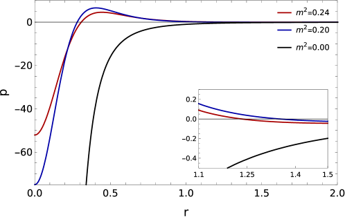
Figure 8: Plot of $p$ vs. $r$ for different values of $m^{2}$. Blue and red lines represent $p$ having $m^{2}$ value in the range $0<m^{2}\leq 0.25$. The black curve is for the singular metric

It is evident from the equation above and by looking at the Figure 8 that SEC is met in the range $(4m^{2}-\sqrt{13}m^{2})b_{0}^{2}\leq r^{2}\leq(4m^{2}+\sqrt{13}m^{2})b_{0}^{2}$. In contrast, the singular RN metric ($m^{2}=0$) violates the SEC for every $r$. Thus, though not globally, our regular black hole satisfies the SEC at least over a specific range of $r$.

$\bullet$ Dominant Energy Condition: The DEC comprises of the inequalities $\rho\geq 0$, $\rho-|\tau|\geq 0$, and $\rho-|p|\geq 0$. In the above discussion, we showed that $\rho\geq 0$ for $r^{2}\leq 3m^{2}b_{0}^{2}$. From eq.(15-16) one can write,

$$\rho-|\tau|=\begin{cases}0,&\text{if }r^{2}\leq 3m^{2}b_{0}^{2}\\ -\frac{2(r^{2}-3g^{2})b_{0}^{2}}{\kappa(r^{2}+g^{2})^{3}},&\text{if }r^{2}>3m^{2}b_{0}^{2}\end{cases}$$ (20)

Hence, $\rho-|\tau|\geq 0$ is satisfied in the range $r^{2}\leq 3m^{2}b_{0}^{2}$, which is also shown in Figure 9(left). To check the third inequality in DEC, we directly use Figure 9(right). It is easy to see that

$$\rho-|p|=\begin{cases}+\text{ve},&\text{if }r^{2}\leq m^{2}b_{0}^{2}\\ -\text{ve},&\text{if }r^{2}>m^{2}b_{0}^{2}\end{cases}$$ (21)

Therefore, we have $\rho\geq 0$, $\rho-|\tau|\geq 0$ for $r^{2}\leq 3m^{2}b_{0}^{2}$ and $\rho-|p|\geq 0$ in the range $r^{2}\leq m^{2}b_{0}^{2}$. Hence, the matter for our regular black hole satisfies the DEC in the range $r^{2}\leq m^{2}b_{0}^{2}$.

Following the above description of energy conditions, the characteristics of the matter needed to maintain our regular black hole may be summed up as follows:

Energy condition	Range of validation
NEC	$r^{2}\leq 5m^{2}b_{0}^{2}$
WEC	$r^{2}\leq 3m^{2}b_{0}^{2}$
SEC	$(4-\sqrt{13})m^{2}b_{0}^{2}\leq r^{2}\leq(4+\sqrt{13})m^{2}b_{0}^{2}$
DEC	$r^{2}\leq m^{2}b_{0}^{2}$

As a result, we find out that our regular black hole solution fulfils all the energy conditions imposed by classical GR in the range $(4-\sqrt{13})m^{2}b_{0}^{2}\leq r^{2}\leq m^{2}b_{0}^{2}$. However, the singular RN type metric $(m^{2}=0)$ violates each and every energy condition across the whole range of $r$.

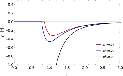
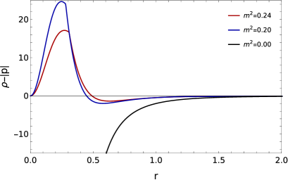
Figure 9: Plot of $\rho-|\tau|$ with $r$ for different values of $m^{2}$(left). Variation of $\rho-|p|$ with $r$ for different values of $m^{2}$(right)

III Matter sources of our geometries

We now turn to the question of constructing sources that may be used to model the matter stress-energy required to support the spacetimes mentioned above. Sources for regular black hole spacetimes have been constructed using nonlinear electrodynamics, scalar fields, and phantom scalar fields Ayon1 ; Ayon2 ; Ayon3 ; Ayon4 ; Ayon5 ; Bronikov2 ; Bronnikov5 ; Bronnikov6 . Though some of the sources may be physically questionable, they do provide some decent examples of Lagrangian-based matter sources for regular geometries. Let us now try and see what could be the possible sources for our geometries. The necessity of ‘exotic matter fields’ is evident from the analysis of energy conditions studied in the earlier section. The well-known Bardeen and Hayward regular black holes have been interpreted as gravitational fields generated by a nonlinear magnetic monopole, as constructed in Ayon4 ; Fan . However, the Lagrangian describing the dynamics of the fields $(\mathbf{F})$ are different in the above two cases, i.e. we don’t have a single well-defined Lagrangian for both. A more general matter Lagrangian for Bardeen and Hayward spacetimes (as well as others) is presented in Zhong . It is given as

$$\mathcal{L(\mathbf{F})}=\frac{4\mu}{\delta}\frac{(\delta\,\mathbf{F})^{\frac{\nu+3}{4}}}{(1+(\delta\,\mathbf{F})^{\frac{\nu}{4}})^{\frac{\mu+\nu}{\nu}}}$$ (22)

where $\mu>0$, $\nu>0$ are dimensionless constants and $\delta>0$ has the dimension of length squared. One obtains a source for the Bardeen metric for $\mu=3,\nu=2$ and for the Hayward metric for $\mu=\nu=3$. The matter sources arising from the above Lagrangian satisfy the null energy condition and violate the strong energy condition. Though, in our case, we have a violation of the null energy condition, our spacetime geometry, as well as the well–known regular black holes satisfy a common relation for the required stress energy, namely $\rho+\tau=0$. In addition, we also have the equality of tangential pressures arising out of spherical symmetry. Below we have depicted two probable sources for our geometries: a non-linear electrodynamic field and another using ideas from braneworld gravity.

III.1 Nonlinear electrodynamics

Motivated by the above discussion, we consider a non-linear electromagnetic field Lagrangian as a source for our regular black hole metric. We show in eq.(15-16) how one can decompose the diagonal elements of the stress-energy tensor in two parts – one satisfying the NEC, WEC, and the other violating them. Interestingly, both parts of the decomposition satisfy $\rho+\tau=0$ separately. One may therefore propose a non-linear electromagnetic field Lagrangian $\mathcal{L}=\mathcal{L}_{1}(\mathbf{F})+\mathcal{L}_{2}(\mathbf{F})$ minimally coupled to gravity by the following action,

$$S=\int d^{4}x\sqrt{-g}\left(\frac{R}{\kappa}-\mathcal{L}_{1}(\mathbf{F})-\mathcal{L}_{2}(\mathbf{F})\right),$$ (23)

where $R$ is the Ricci scalar. $\mathcal{L}_{1}(\mathbf{F})$ is the non-linear electromagnetic Lagrangian which generates an energy–momentum tensor violating the NEC, WEC. $\mathcal{L}_{2}(\mathbf{F})$, in contrast, leads to a ${T_{\mu\nu}}$ which satisfies the WEC, NEC. Here, $F_{\mu\nu}$ is electromagnetic strength tensor and $\mathbf{F}\equiv F^{\mu\nu}F_{\mu\nu}$.

The covariant equations of motion (field variation and metric variation) which emerge from the above Lagrangian are given as,

$$\nabla_{\mu}\left(\frac{\partial\mathcal{L}_{(i)}}{\partial\mathbf{F}}F^{\mu\nu}\right)=0;\hskip 11.38092pti=1,2$$ (24)

$$R_{\mu\nu}-\frac{1}{2}g_{\mu\nu}R=\kappa\mathbf{T}_{\mu\nu}=\kappa\sum_{i=1}^{2}T_{\mu\nu}^{(i)}$$ (25)

where $R_{\mu\nu}$ is the Ricci tensor. $T_{\mu\nu}^{(1)}$ and $T_{\mu\nu}^{(2)}$ are energy-momentum tensors corresponding to $\mathcal{L}_{1}(\mathbf{F})$ and $\mathcal{L}_{2}(\mathbf{F})$, respectively. One can write the two energy-momentum tensors in the following fashion,

$$T_{\mu\nu}^{(i)}=2\left(\frac{\partial\mathcal{L}_{(i)}}{\partial\mathbf{F}}F_{\mu\alpha}F_{\nu}{}^{\alpha}-\frac{1}{4}g_{\mu\nu}\mathcal{L}_{(i)}(\mathbf{F})\right);\hskip 5.69046pti=1,2$$ (26)

From eq.(15-16), it is clear that we need a matter source that has isotropic tangential pressures and satisfies $\rho+\tau=0$. As a result, we only have non-zero components of the electromagnetic strength tensor $F_{tr}$ and $F_{\theta\phi}$ to serve this purpose.

Hence, in the frame basis, the diagonal elements of the total energy-momentum tensor take the following form:

$$\mathbf{T}_{00}= -\mathbf{T}_{11}=\sum_{i=1}^{2}\left(\frac{1}{2}\mathcal{L}_{(i)}(\mathbf{F})-2\frac{\partial\mathcal{L}_{(i)}}{\partial\mathbf{F}}F_{tr}F^{tr}\right);$$ (27)

$$\mathbf{T}_{22}= \mathbf{T}_{33}=\sum_{i=1}^{2}\left(-\frac{1}{2}\mathcal{L}_{(i)}(\mathbf{F})+2\frac{\partial\mathcal{L}_{(i)}}{\partial\mathbf{F}}F_{\theta\phi}F^{\theta\phi}\right)$$ (28)

It is evident from the above that for any ${\cal L}(\mathbf{F})$, one does have $\rho+\tau=0$ and isotropic tangential pressures. From the Einstein tensor components evaluated earlier in the frame basis and noticing the split as shown in eq.(15-16), one can write

$$\frac{1}{2}\mathcal{L}_{1}(\mathbf{F_{0}})-2F_{tr}F^{tr}\left(\frac{\partial\mathcal{L}_{1}}{\partial\mathbf{F}}\right)_{\mathbf{F}=\mathbf{F}_{0}}= -\frac{b_{0}^{2}r^{2}}{\kappa(r^{2}+g^{2})^{3}};$$ (29)

$$-\frac{1}{2}\mathcal{L}_{1}(\mathbf{F_{0}})+2F_{\theta\phi}F^{\theta\phi}\left(\frac{\partial\mathcal{L}_{1}}{\partial\mathbf{F}}\right)_{\mathbf{F}=\mathbf{F_{0}}}= -\frac{b_{0}^{2}r^{2}(r^{2}-2g^{2})}{\kappa(r^{2}+g^{2})^{4}};$$ (30)

$$\frac{1}{2}\mathcal{L}_{2}(\mathbf{F_{0}})-2F_{tr}F^{tr}\left(\frac{\partial\mathcal{L}_{2}}{\partial\mathbf{F}}\right)_{\mathbf{F}=\mathbf{F}_{0}}= +\frac{3g^{2}b_{0}^{2}}{\kappa(r^{2}+g^{2})^{3}};$$ (31)

$$-\frac{1}{2}\mathcal{L}_{2}(\mathbf{F_{0}})+2F_{\theta\phi}F^{\theta\phi}\left(\frac{\partial\mathcal{L}_{2}}{\partial\mathbf{F}}\right)_{\mathbf{F}=\mathbf{F_{0}}}= -3g^{2}\frac{b_{0}^{2}(g^{2}-2r^{2})}{\kappa(r^{2}+g^{2})^{4}};$$ (32)

where the LHS in the above equations are evaluated on-shell, i.e. for a specific solution $\mathbf{F}=\mathbf{F_{0}}$, which, of course, has to satisfy the field equations.

Let us assume that for specific values of parameters, a combination of the following two non-linear electrodynamic field Lagrangian densities can support our regular black holes;

$$\mathcal{L}_{1}(\mathbf{F})=-\frac{\gamma\mathbf{F}}{\left(1+\eta\sqrt{\mathbf{F}}\right)^{3}};\hskip 22.76228pt\mathcal{L}_{2}(\mathbf{F})=\frac{3\gamma\eta\mathbf{F}^{3/2}}{\Big{(}1+\eta\sqrt{\mathbf{F}}\Big{)}^{3}}$$ (33)

where $\gamma$ and $\eta$ are two separate constants. Therefore, one might have distinct field dynamics based on the different $\gamma$ and $\eta$ options. For our purposes, we select just a magnetic solution with $\mathbf{F_{0}}=2F_{\theta\phi}F^{\theta\phi}=\frac{2q_{m}^{2}}{r^{4}}$, $\gamma=b_{0}^{2}/\kappa q_{m}^{2}$, and $\eta=g^{2}/\sqrt{2q_{m}^{2}}$, which satisfy eq.(29-32), where $q_{m}^{2}$ is an arbitrarily chosen constant.

Therefore, the total non-linear electrodynamic field Lagrangian density can be written as a combination of the above two in the following way;

$$\mathcal{L}(\mathbf{F})=-\frac{\gamma\mathbf{F}(1-3\eta\sqrt{\mathbf{F}})}{\Big{(}1+\eta\sqrt{\mathbf{F}}\Big{)}^{3}}$$ (34)

Note that for $g^{2}=0$ or $\eta=0$, i.e. singular RN type solution, the matter source becomes;

$$\mathcal{L}(\mathbf{F})=-\gamma\mathbf{F}$$ (35)

Thus, the singular RN-type solution with imaginary charge is sourced by a linear magnetic Lagrangian density. The source Lagrangian of equation (34) has the limitation that it cannot allow negative $\mathbf{F}$ values since it contains fractional powers of $\mathbf{F}$. Therefore, we are limited to working with positive $\mathbf{F}$ values.

It is known that our regular black holes are made up of the two parameters $b_{0}^{2}$ and $g^{2}$. However, the NED source Lagrangian depends on an additional free parameter, $q_{m}^{2}$. Thus, to comprehend $q_{m}^{2}$ and the behaviour of the source current that creates this type of magnetic field, we must investigate the dynamics of the source Lagrangians.

The functional value of $\mathbf{F_{0}}$ makes it clear that $F_{\theta\phi}=-q_{m}\sin{\theta}$. And, in the curved space, the non-linear Maxwell-like equations that follow from the Lagrangians mentioned above, with source current, may also be expressed as,

$$\nabla_{\mu}F^{\mu\nu}+\left(\frac{\partial^{2}\mathcal{L}_{(i)}}{\partial\mathbf{F}^{2}}\bigg{/}\frac{\partial\mathcal{L}_{(i)}}{\partial\mathbf{F}}\right)(\partial_{\mu}\mathbf{F})F^{\mu\nu}=J^{\nu}_{e}{}_{(i)}$$ (36)

$$\nabla_{\mu}\tilde{F}^{\mu\nu}=J^{\nu}_{m}$$ (37)

where $\tilde{F}^{\mu\nu}\equiv\frac{1}{2}\epsilon^{\mu\nu\rho\sigma}F_{\rho\sigma}$ ($\epsilon^{\mu\nu\rho\sigma}$ is the Levi-Civita tensor), the dual of field strength tensor. For the derived field strength tensor $F_{\theta\phi}$, we find that $J^{\nu}_{e}=\{0,0,0,0\}$ and $J^{\nu}_{m}=\{\rho_{m},0,0,0\}$ (where, $\rho_{m}=q_{m}\delta^{3}(r)$) independent of the form of source Lagrangian. Therefore, it is also valid for the total electrodynamic field Lagrangian $(\mathcal{L}(\mathbf{F}))$. Thus, a non-linear magnetic monopole at $r=0$ supports our regular black hole, with $q_{m}$ being the total magnetic charge.

III.2 Braneworld gravity

As stated earlier, we may consider our regular black hole geometry in the context of Brane-World Gravity Maartens . To facilitate this, let us introduce a new kind of decomposition of the energy-momentum tensor components in eq.(15-16).

$$\rho=-\tau=-\frac{b_{0}^{2}r^{2}}{\kappa(r^{2}+g^{2})^{3}}+\frac{3g^{2}b_{0}^{2}}{\kappa(r^{2}+g^{2})^{3}}=\rho_{t}+\rho_{e}$$ (38)

$$p=-\frac{b_{0}^{2}r^{2}}{\kappa(r^{2}+g^{2})^{3}}-3g^{2}b_{0}^{2}\frac{(g^{2}-3r^{2})}{\kappa(r^{2}+g^{2})^{4}}=p_{t}+p_{e}$$ (39)

One may note that we have chosen a decomposition such that a part of the energy-momentum tensor is traceless. The rest of the energy-momentum is non-zero only when $g\neq 0$ and it satisfies the NEC, WEC, as is evident from the Figure 10. We can exploit this decomposition as follows. Recall the well-known effective Einstein equations on the four-dimensional 3-brane. They are written as

$$G_{\mu\nu}=-\Lambda g_{\mu\nu}+\kappa T_{\mu\nu}+6\frac{\kappa}{\lambda}S_{\mu\nu}-\mathcal{E}_{\mu\nu}$$ (40)

where $\Lambda$ is a four dimensional cosmological constant on the 3-brane, $T_{\mu\nu}$ is the on-brane matter, $S_{\mu\nu}$ is the so-called quadratic stress energy on the brane. The traceless $\mathcal{E}_{\mu\nu}$ is a geometric quantity controlled by the extra dimension and related to the Weyl tensor of the bulk five-dimensional spacetime. If we assume a large brane tension $\lambda$ and a zero $\Lambda$, the terms involving $S_{\mu\nu}$ drop out, and we are left with only the $\mathcal{E}_{\mu\nu}$, which can be used to model the traceless part in the expressions in (38), (39). Note that the negativity of $\rho_{t}$ and $p_{t}$ is already accounted for through the negative sign in front of the $\mathcal{E}_{\mu\nu}$ term in the effective Einstein equations in (40). The remaining part, i.e. the $\rho_{e}$ and $p_{e}$ can be adjusted into the ‘on-brane matter’ described through $T_{\mu\nu}$.

As is known, the RN spacetime with negative $Q^{2}$ was used as one of the first solutions of the effective Einstein equations on the brane (see Maartens and references therein). Here, our regularisation of the geometry seems to add an extra on-brane matter which is well-behaved insofar as energy conditions are concerned.

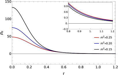
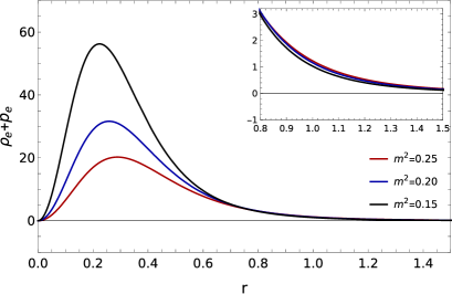
Figure 10: (Left) Plot of $\rho_{e}$ with $r$ shows a positive definite energy density of the extra matter part. (Right) Plot of $\rho_{e}+p_{e}$ with $r$, which is also positive for all values of $r$.

IV Shadow radius and observational bounds

The strong gravitational field around a black hole causes photons to be deflected or absorbed, which results in a silhouette which is also termed as the black hole shadow. Each black hole has a unique shape and size for its shadow, which is controlled by parameters appearing in its geometry (i.e. metric parameters such as mass, charge, angular momentum etc.). Originally, Bardeen bardeenshadow introduced (assuming the observer very far away) celestial coordinates in the observer’s sky to describe and quantify the shadow. More recently, there have been attempts wherein shadows have been calculated using ray tracing methods for observers (moving or static) at a finite distance or in asymptotically non-flat scenarios Volker .

The shadow of a black hole may be seen as a dark region surrounded by photon rings. Photons with less angular momentum scatter from the black hole and may be seen from infinity; photons with higher angular momentum enter the black hole and leave a dark circle. As mention above, two celestial coordinates, $\alpha$ and $\beta$, were introduced by Bardeen which are,

$$\alpha=\lim_{r_{0}\to\ \infty}\Big{(}-r_{0}^{2}\sin{\theta_{0}}\frac{d\phi}{dr}\Big{)};\hskip 28.45274pt\beta=\lim_{r_{0}\to\ \infty}r_{0}^{2}\frac{d\theta}{dr}$$ (41)

where $r_{0}$ is the distance between the black hole and the observer, $\theta_{0}$ is the inclination angle between the black hole rotation axis and the line of sight between the source and observer. The derivatives $\frac{d\theta}{dr}$ and $\frac{d\phi}{dr}$ have to be evaluated in the asymptotic region using the first integrals of the geodesic equations. The radius of the static spherically symmetric black hole shadow, $r_{sh}$, as viewed by a static observer at radial coordinate $r_{0}$, may be approximated as Volker :

$$r_{sh}^{2}=\alpha^{2}+\beta^{2}=\frac{r_{ph}^{2}}{w(r_{ph})}$$ (42)

where $r_{ph}$ is the radius of photon sphere and $w(r)=-g_{tt}(r)$. For a static spherically symmetric black hole, the photon sphere is the orbit at which light moves in an unstable circular null geodesic Virbhadra . The equations of motion for photons around a static and spherically symmetric black hole environment can be obtained using the Hamilton-Jacobi or Hamiltonian formulations, as described in Chen , which then enables one to determine the effective potential defining the system. The radius of the photon sphere $r_{ph}$ can be calculated from the critical point conditions of this effective potential by solving the expression

$$\frac{r_{ph}w^{{}^{\prime}}(r_{ph})}{w(r_{ph})}=2$$ (43)

where a prime denotes a derivative with respect to the radial coordinate.

IV.1 Shadow radius of our regular black hole

Based on the description above, we first need to know the radius of the photon sphere in order to calculate the shadow radius of our black hole. The equation for the radius of the photon sphere can be obtained by substituting $w(r)=1-\frac{b_{0}^{2}r^{2}}{(r^{2}+g^{2})^{2}}$ in equation (43), which gives,

$$(r_{ph}^{2}+m^{2}b_{0}^{2})^{3}-2r_{ph}^{4}b_{0}^{2}=0$$ (44)

where we use our special parametrization $g^{2}=m^{2}b_{0}^{2}$. The above expression represents a cubic algebraic equation in the variable $r_{ph}^{2}$. To analyse the characteristics of the roots, it is convenient to express the cubic equation in $r_{ph}^{2}$ in the depressed cubic form and examine its discriminant. We have checked (not shown here) through plots that the discriminant of the cubic equation turns out to be positive or equal to zero for values of $m^{2}$ within the range of $0$ to $0.296$. This observation provides confirmation that there are three distinct real roots for $r_{ph}^{2}$ within the specified range of $m^{2}$. Hence, within the specified interval of $m^{2}$, it is possible to obtain two positive real roots, two negative real roots, and two imaginary roots for $r_{ph}$. We take into consideration the two real positive roots as potential candidates for the photon sphere since they lie inside the domain of coordinates. An unstable circular orbit may now be found at one of these two roots by performing a stability analysis on the effective potential, which is defined as,

$$V_{eff}(r)=\Big{(}1-\frac{b_{0}^{2}r^{2}}{(r^{2}+m^{2}b_{0}^{2})^{2}}\Big{)}\frac{L^{2}}{r^{2}}$$ (45)

Here $L$ is the angular momentum of the photon. Let us say $\bar{r}_{ph}$ is the location of the unstable circular orbit. Hence, the shadow radius from eq.(42) becomes;

$$r_{sh}^{2}=\frac{\bar{r}_{ph}^{2}(\bar{r}_{ph}^{2}+m^{2}b_{0}^{2})^{2}}{(\bar{r}_{ph}^{2}+m^{2}b_{0}^{2})^{2}-\bar{r}_{ph}^{2}b_{0}^{2}}$$ (46)

In section II, it has been demonstrated that a horizon exists for values of $m^{2}$ such that $0<m^{2}\leq 0.25$. In this specified interval of $m^{2}$, we find that $\bar{r}_{ph}$ can vary between $1.141b_{0}>\bar{r}_{ph}\geq 1.029b_{0}$. However, for $0.25<m^{2}\leq 0.296$, there is no horizon but a photon sphere exists, i.e. we have a regular spacetime having a photon sphere which may be used to model a compact object. In addition, the asymptotic observer can estimate the angular diameter of the shadow as follows: $2\alpha_{D}=2r_{sh}/r_{0}$ Volker .

IV.2 Constraints from the observed shadow of M87* and Sgr A*

Even though astrophysical black holes rotate and the shape of the shadow is controlled by the rotation parameter, one can still use the circular shadow of a static and spherically symmetric black hole to estimate parameters roughly. In addition, the shadows for M87^∗ and Sgr A^∗ are reported to be close to being circular. This motivates us to identify and check possible observational traces of our regular black hole in the supermassive compact objects in M87^∗ and Sgr A^∗. We will use freely available EHT results in order to arrive at our estimates.

In this section, we have estimated the metric parameter $b_{0}$ for different $m^{2}$ values using the shadows observed by EHT. It is important to keep in mind that our theoretical angular diameter is based on the black hole parameters $b_{0}$, $m^{2}$, and the black hole to observer’s distance, $r_{0}$. Therefore, to estimate the other parameter $b_{0}$ from the observed angular diameter data, one requires an independent measurement of the distance $(r_{0})$ and a hand-picked value of $m^{2}$.

In the 2019 EHT reports, the observed angular diameter of black hole M87^∗ at the centre of the galaxy M87 is $\Phi=(42\pm 3)\mu as$ Akiyama1 ; Akiyama2 ; Akiyama3 ; Akiyama4 ; Akiyama5 ; Akiyama6 . Recently, the original EHT data was more thoroughly analysed in Medeiros , and they obtained $\Phi=41.5\pm 0.6\mu as$. We estimate our metric parameters using both results. According to stellar population measurement, M87^∗ is located at a distance of $r_{0}=(16.8\pm 0.8)Mpc$ Blakeslee ; Bird ; Cantiello . However, the error bar of the distance measurements has been disregarded for our purposes. Therefore, the following are possible ways to describe the theoretical angular diameter of M87^∗:

$$2\alpha_{D}=8189.26\times 10^{-16}\sqrt{\frac{\bar{r}_{ph}^{2}(\bar{r}_{ph}^{2}+m^{2}b_{0}^{2})^{2}}{(\bar{r}_{ph}^{2}+m^{2}b_{0}^{2})^{2}-\bar{r}_{ph}^{2}b_{0}^{2}}}\hskip 10.84006pt\mu as$$ (47)

where we have substituted $r_{0}=16.8Mpc$. Now, one may calculate $\bar{r}_{ph}$ for a given value of $m^{2}$ using the photon sphere equation (44) and by the stability analysis of the effective potential. Substituting $\bar{r}_{ph}$ in equation (47), we have the theoretical angular diameter of the shadow as a function of $b_{0}$. Thus, one may estimate $b_{0}$ by comparing the theoretical prediction with observed data. In Figure [11], we have shown a 2D plot of $(m^{2},b_{0})$ values. The shaded region contains permissible values of $(m^{2},b_{0})$ based on the observed angular diameter of the shadow of M87^∗ with its associated uncertainty, as per the observed data reported in Akiyama1 ; Akiyama2 ; Akiyama3 ; Akiyama4 ; Akiyama5 ; Akiyama6 ; Medeiros .

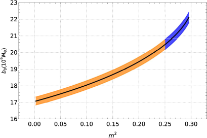
Figure 11: The above figures demonstrate the variation of $b_{0}$ with $m^{2}$ for the observed angular diameter of M87^∗, considering both analyses of shadow diameter reported as $42\pm 3\mu as$ (left) and $41.5\pm 0.6\mu as$ (right)

As mentioned above, we have shown two plots corresponding to the two data analyses of the same EHT data of M87^∗. The central two black lines represent the set of values of $(m^{2},b_{0})$ corresponding to the angular diameter $42\mu as$ (Fig. 11(left)) and $41.5\mu as$ (Fig. 11(right)), respectively. The error in the measurement of the angular diameter is also considered and has been shown with orange and blue shaded regions in the parameter space. For the angular diameter $(42\pm 3)\mu as$, in Figure 11(left), the orange-shaded region corresponds to the regular black hole $(0<m^{2}\leq 0.25)$ having the value of metric parameter $b_{0}$ between $16.05\times 10^{9}M_{\odot}<b_{0}\leq 22.22\times 10^{9}M_{\odot}$ and the blue shaded region depicts the values of $(m^{2},b_{0})$ to represent horizonless compact object $(0.25<m^{2}\leq 0.296)$. Assuming the angular diameter as $41.5\pm 0.6\mu as$, in Figure 11(right), the value of $b_{0}$ for the regular black hole varies between $16.83\times 10^{9}M_{\odot}<b_{0}<20.78\times 10^{9}M_{\odot}$. The horizonless compact object can also model the same data, which are represented in the blue shaded region of Figure 11(right).

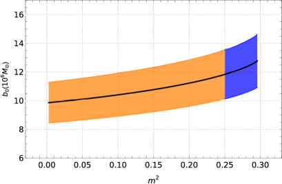
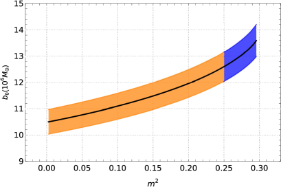
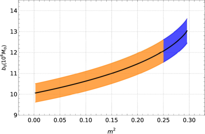
Figure 12: Above figures illustrate the variation of $b_{0}$ with $m^{2}$ for angular diameter of Sgr A^∗, considering both shadow diameter $48.7\pm 7\mu as$ (top left and bottom left) and emission ring diameter $51.8\pm 2.3\mu as$ (top right and bottom right), while distances are taken to be those reported by the Gravity collaboration (top panel) and Keck team (bottom panel).

One can perform a similar exercise with the observed shadow of Sgr A^∗. According to EHT collaboration angular diameter of shadow for Sgr A^∗ is $(48.7\pm 7)\mu as$ and emission ring of Sgr $A^{*}$ has angular diameter $51.8\pm 2.3\mu as$ Akiyama7 ; Akiyama8 ; Akiyama9 ; Akiyama10 ; Akiyama11 ; Akiyama12 . There are several works on the shadow of Sgr A^∗ using either shadow diameter ($48.7\pm 7\mu as$ ) or emission ring diameter ($51.8\pm 2.3\mu as$). Therefore, we estimate the metric parameter $b_{0}$ by analyzing both data sets for completeness. There are several reports on the distance of Sgr A^∗. Keeping the redshift parameter-free, the Keck team reported the distance of Sgr A^∗ to $(7959\pm 59\pm 32)pc$ Do . Considering the redshift parameter unity, the same group reported the distance as $(7935\pm 50)pc$ Do . According to the Gravity collaboration, the distance is $(8246.7\pm 9.3)pc$ Gravity1 ; Gravity2 . By accounting for optical aberrations, the Gravity Collaboration significantly reduced the BH distance to $(8277\pm 9\pm 33)pc$. Figures 12 (top panel) and 12 (bottom panel) represent the parameter space $(m^{2},b_{0})$ corresponding to the observer to Sgr A^∗ distance as reported by Gravity collaboration and Keck team, respectively. Each panel of Figure 12(top, bottom) contains separate analyses of parameter space by assuming both shadow diameter and emission ring diameter of Sgr A^∗. Thus plots of Figure 12 demonstrate how both horizonless compact objects and regular black holes may model the shadow of Sgr A^∗.

As a result, we obtain a collection of points $(m^{2},b_{0})$ that can be used to simulate the angular diameter of the shadows of M87^∗ and Sgr A^∗. These points represent either a regular black hole or a horizonless compact object. In Table 1, we have summarized the limits on $b_{0}$ imposed by the shadows of M87^∗ and Sgr A^∗.

Massive Object	Distance from the observer	Angular Diameter$(\mu as)$	Constraint on $b_{0}$ for regular BH	Constraint on $b_{0}$ for compact object	Unit of $b_{0}$
M87∗	$16.8$ Mpc (Stel. popula. measure.)	$42\pm 3$	$16.05<b_{0}\leq 22.22$	$19.26<b_{0}\leq 24.01$	$10^{9}M_{\odot}$
		$41.5\pm 0.6$	$16.83<b_{0}\leq 20.78$	$20.19<b_{0}\leq 22.46$
Sgr A∗	$8277$ pc (Gravity Collab.)	$48.7\pm 7$	$8.46<b_{0}\leq 13.55$	$10.14<b_{0}\leq 14.64$	$10^{6}M_{\odot}$
		$51.8\pm 2.3$	$10.03<b_{0}\leq 13.16$	$12.04<b_{0}\leq 14.22$
	$7935$ pc (Keck team)	$48.7\pm 7$	$8.11<b_{0}\leq 12.99$	$9.72<b_{0}\leq 14.03$
		$51.8\pm 2.3$	$9.62<b_{0}\leq 12.61$	$11.54<b_{0}\leq 13.63$

Table 1: Limit on $b_{0}$ from the angular diameter of shadows of M87^∗ and Sgr A^∗

V Conclusion

We will now review our findings and make a few remarks to wrap up our work.

1. We discuss the GR singularity problem and propose a novel spacetime model which, based on the metric parameters, corresponds to singular, regular black holes or horizon-less compact objects. The line element we work with is restated here:

   $$ds^{2}=-\Big{(}1-\frac{b_{0}^{2}r^{2}}{(r^{2}+g^{2})^{2}}\Big{)}dt^{2}+\Big{(}1-\frac{b_{0}^{2}r^{2}}{(r^{2}+g^{2})^{2}}\Big{)}^{-1}dr^{2}+r^{2}\Big{(}d\theta^{2}+\sin^{2}\theta d\phi^{2}\Big{)}.$$

   Throughout our discussion, we used a specific parametrization, namely $m^{2}=g^{2}/b_{0}^{2}$. Depending on the values of $m^{2}$, different classes of geometries can be constructed from the model mentioned above. For $m^{2}=0$, we have a mutated Reissner–Nordström geometry with an imaginary charge and a vanishing mass parameter. A family of regular black holes having two horizons can be presented when $0<m^{2}\leq 0.25$. When $0.25<m^{2}\leq 0.296$ we have spacetimes representing horizon-less compact objects having photon spheres.

2. The singular RN-type metric $(m^{2}=0)$ violates all the classical energy conditions. However, after regularization, the family of regular black holes $(0<m^{2}\leq 0.25)$ seem to satisfy all the energy conditions in a specific range of $r$, though not everywhere. Further, for the regular black hole family, we have shown that components of the curvature tensor and different curvature scalars are indeed finite everywhere. Following a different path Modesto , we have also confirmed that the regular black hole family is geodesically complete for massive and massless test particles.

3. We found that the family of regular black holes and the horizonless compact objects can be interpreted as the gravitational field sourced by a minimally coupled nonlinear magnetic monopole. The total stress energy can be divided into two parts; one satisfying NEC and WEC and the other violating them. The source of the singular RN-type metric $(m^{2}=0)$ may be chosen as a linear magnetic monopole. As we mentioned in the Introduction, it remains a concern that the source of a regular black hole requires modelling using a nonlinear electromagnetic field. This deficiency needs to be remedied through further explorations in future. We have also shown how the matter required for our geometry may also be modelled using braneworld gravity.

4. Finally, we present the shadow radius of the regular black hole. Comparing with the observed EHT collaboration results, we find that both M 87^∗ and Sgr A^∗ can indeed be modelled by our regular black hole corresponding to particular values for the set $(b_{0}^{2},m^{2})$. Interestingly, one can also model the data by a horizon-less compact object ($0.25<m^{2}\leq 0.296$).

In conclusion, we have found regular spacetimes with and without horizons, sourced by a nonlinear magnetic monopole, which may be used to model the supermassive compact objects as well as ordinary compact objects, which seem to be abundant in different galaxies in the universe.

It may be possible to extend our work to include line elements where a Bardeen–like regularising term is added in the metric functions $-g_{tt}$ or $(g_{rr})^{-1}$. The consequences of such an addition may be explored. We can also see if the ultrastatic spacetimes ($g_{tt}=-1$), which arise assuming the same $g_{rr}$ have nonsingular wormhole features. The status of energy conditions and, more importantly, the question of viable matter sources need to be addressed in such scenarios in order to facilitate a proper understanding. We hope to return to such issues in future.

References

- (1) B. P. Abbott et al., Phys. Rev. Lett. 116, 061102 (2016).
- (2) B. P. Abbott et al., Phys. Rev. Lett. 116, 241103 (2016).
- (3) B. P. Abbott et al., Phys. Rev. Lett. 118, 221101 (2017).
- (4) B. P. Abbott et al., Phys. Rev. Lett. 119, 161101 (2017).
- (5) K. Akiyama et al., Astrophys. J. Lett. 875, L1 (2019).
- (6) K. Akiyama et al., Astrophys. J. Lett. 875, L2 (2019).
- (7) K. Akiyama et al., Astrophys. J. Lett. 875, L3 (2019).
- (8) K. Akiyama et al., Astrophys. J. Lett. 875, L4 (2019).
- (9) K. Akiyama et al., Astrophys. J. Lett. 875, L5 (2019).
- (10) K. Akiyama et al., Astrophys. J. Lett. 875, L6 (2019).
- (11) K. Akiyama et al., Astrophys. J. Lett. 930, L12 (2022).
- (12) K. Akiyama et al., Astrophys. J. Lett. 930, L13 (2022).
- (13) K. Akiyama et al., Astrophys. J. Lett. 930, L14 (2022).
- (14) K. Akiyama et al., Astrophys. J. Lett. 930, L15 (2022).
- (15) K. Akiyama et al., Astrophys. J. Lett. 930, L16 (2022).
- (16) K. Akiyama et al., Astrophys. J. Lett. 930, L17 (2022).
- (17) S.W. Hawking and G.F.R. Ellis, The Large Scale Structure of Spacetime (Cambridge University Press, Cambridge 1973).
- (18) S. Ansoldi, in Conference on Black Holes and Naked Singularities, Milano, Italy, 2007, arXiv: 0802.0330 [gr-qc].
- (19) O. B. Zaslavskii, Phys. Lett. B 688, 278–280 (2010).
- (20) A. D. Sakharov, Zh. Eksp. Teor. Fiz. 49, 345 (1966) [Sov. Phys. JETP 22, 241 (1966)].
- (21) E. B. Gliner, Sov. Phys. JETP 22, 378 (1966).
- (22) J. M. Bardeen, in Proceedings of International Conference GR5, Tbilisi, USSR, 1968, p. 174.
- (23) J.M. Bardeen, arXiv:1406.4098
- (24) J.M. Bardeen, arXiv:1811.06683.
- (25) S. A. Hayward, Phys. Rev. Lett. 96, 031103 (2006).
- (26) T.A. Roman and P.G. Bergmann, Phys. Rev. D 28 1265 (1983).
- (27) I. Dymnikova, Gen. Relativ. Gravit. 24, 235 (1992).
- (28) I. Dymnikova, Int. J. Mod. Phys. D 12, 1015(2003).
- (29) E. Ayon-Beato and A. Garcia, Phys. Rev. Lett. 80, 5056 (1998).
- (30) E. Ayon-Beato and A. Garcia, Phys. Lett. B 464, 25 (1999).
- (31) V.P. Frolov, Phys. Rev. D 94, 104056 (2016).
- (32) V.P. Frolov, J. High Energ. Phys. 05, 049 (2014).
- (33) V.P. Frolov and A. Zelnikov, Phys. Rev. D 95, 124028 (2017).
- (34) L. Balart and E. C. Vagenas, Phys. Rev. D 90, 124045 (2014).
- (35) K. A. Bronnikov, Phys. Rev. D 63, 044005 (2001).
- (36) A. Simpson and M. Visser, J. Cosmol. Astropart. Phys. 02, 042(2019).
- (37) R. Carballo-Rubio, F. Di Filippo, S. Liberati, C. Pacilio and M. Visser, J. High Energ. Phys. 07, 023 (2018).
- (38) R. Carballo-Rubio, F. Di Filippo, S. Liberati and M. Visser, Phys. Rev. D 98, 124009 (2018).
- (39) C. Bambi and L. Modesto, Phys. Lett. B 721, 329 (2013).
- (40) S. G. Ghosh and S. D. Maharaj, Eur. Phys. J. C 75, 7 (2015).
- (41) S. Sajadi, N. Riazi, Gen. Relativ. Gravit. 49, 45(2017).
- (42) P. D. Roy and S. Kar, Phys. Rev. D 106, 044028 (2022).
- (43) K. Pal, K. Pal, P. Roy and T. Sarkar, Eur. Phys. J. C 83, 397 (2023)
- (44) E. Ayon-Beato and A. Garcia, Gen. Relativ. Gravit. 31, 629 (1999).
- (45) E. Ayon-Beato and A. Garcia, Phys. Lett. B 493, 149 (2000).
- (46) E. Ayon-Beato and A. Garcia, Gen. Relativ. Gravit. 37, 635 (2005).
- (47) Z. Y. Fan, Eur. Phys. J. C 77, 266 (2017).
- (48) K. A. Bronnikov, Phys. Rev. Lett. 85, 4641 (2000)
- (49) K. A. Bronnikov, Int. J. Mod. Phys. D 27, 1841005 (2018)
- (50) Z. Y. Fan and X. Wang, Phys. Rev. D 94, 124027 (2016).
- (51) A. Bokulić, I. Smolić, and T. Jurić, Phys. Rev. D 106, 064020 (2022)
- (52) E. Poisson and W. Israel, Phys. Rev. Lett. 63, 1663 (1989).
- (53) E. Poisson and W. Israel, Phys. Rev. D 41, 1796 (1990).
- (54) A. Bonanno, A.-P. Khosravi, and F. Saueressig, Phys. Rev. D 103, 124027 (2021).
- (55) R. Carballo-Rubio, F. Di Filippo, S. Liberati, C. Pacilio and M. Visser, J. Cosmol. Astropart. Phys. 09, 118(2022).
- (56) A. Einstein and N. Rosen, Phys. Rev. 48, 73 (1935).
- (57) S. Weinberg, Gravitation and Cosmology: Principles and Applications of the General Theory of Relativity (John Wiley and Sons, New York, 1972).
- (58) H. W. Hu, C. Lan and Y. G. Miao Lan, arXiv:2303.03931[gr-qc]
- (59) R. M. Wald, General Relativity. Chicago Univ. Pr., Chicago, USA, 1984.
- (60) T. Zhou and L. Modesto, Phys. Rev. D 107, 044016 (2023).
- (61) R. Carballo-Rubio, F. Di Filippo, S. Liberati, and M. Visser, Phys. Rev. D 101, 084047 (2020).
- (62) R. Carballo-Rubio, F. Di Filippo, S. Liberati, and M. Visser, J. High Energ. Phys. 02, 122 (2022).
- (63) K. Pal, K. Pal and T. Sarkar, arXiv: 2307.09382 (2023)
- (64) R. Torres, arXiv:2208.12713 [gr-qc]
- (65) B. Toshmatov, C. Bambi, B. Ahmedov, A. Abdujabbarov, and Z. Stuchlik, Eur. Phys. J. C 77, 542 (2017).
- (66) C. Lan, Y.-G. Miao, and Y.-X. Zang, Eur. Phys. J. C 82, 231 (2022).
- (67) K. A. Bronnikov, Particles 1, 5 (2018).
- (68) K. A. Bronnikov and J. C. Fabris, Phys. Rev. Lett. 96, 251101 (2006).
- (69) K. A. Bronnikov and R. K. Walia, Phys. Rev. D 105, 044039 (2022).
- (70) R. Maartens and K. Koyama, Living Rev. Relativ. 13, 5 (2010).
- (71) J.M. Bardeen, in Black Holes (Les Astres Occlus), ed. C. DeWitt and B. S. DeWitt (New York: Gordon and Breach), 215 (1973).
- (72) V. Perlick and O. Y. Tsupko, Phys. Rep. 947, 1-39 (2022).
- (73) C. M. Claudel, K.S. Virbhadra, G.F.R. Ellis, J.Math.Phys. 42, 818-838 (2001)
- (74) D. Chen, C. Gao, X. Liu, and C. Yu, Eur. Phys. J. C, 81, 700 (2021).
- (75) L. Medeiros et al., Astrophys. J. Lett. 947, L7 (2023).
- (76) J. P. Blakeslee et al., Astrophys. J. Lett. 694, 556–572 (2009).
- (77) S. Bird, W. E. Harris, J. P. Blakeslee, and C. Flynn, Astron. Astrophys. 524, A71 (2010).
- (78) M. Cantiello et al., Astrophys. J. Lett. 854, L31 (2018).
- (79) T. Do et al., Science 365 no. 6454, 664–668 (2019).
- (80) R. Abuter et al., Astron. Astrophys. 657, L12 (2022).
- (81) R. Abuter et al., Astron. Astrophys. 636, L5 (2020).