Quantum many-body scars in the Bose-Hubbard model with a three-body constraint

Abstract

We uncover the exact athermal eigenstates in the Bose-Hubbard (BH) model with a three-body constraint, motivated by the exact construction of quantum many-body scar (QMBS) states in the $S=1$ $XY$ model. These states are generated by applying an $\rm SU(2)$ ladder operator consisting of a linear combination of two-particle annihilation operators to the fully occupied state. By using the improved Holstein-Primakoff expansion, we clarify that the QMBS states in the $S=1$ $XY$ model are equivalent to those in the constrained BH model with additional correlated hopping terms. We also find that, in the strong-coupling limit of the constrained BH model, the QMBS state exists as the lowest-energy eigenstate of the effective model in the highest-energy sector. This fact enables us to prepare the QMBS states in a certain adiabatic process and opens up the possibility of observing them in ultracold-atom experiments.

Introduction. Recent technological developments in ultracold atoms in optical lattices [1], Rydberg atoms in optical-tweezer arrays [2], trapped-ion systems [3], and superconducting qubit systems [4] allow for simulating dynamics in isolated quantum many-body systems and enable us to observe thermalization in sufficiently large systems in experiments. One of the important concepts that partly explains how isolated quantum many-body systems thermalize is the strong eigenstate thermalization hypothesis (strong ETH) [5, 6, 7]. It claims that, for all eigenstates of the quantum many-body Hamiltonian, the expectation value of a local operator coincides with that of the microcanonical ensemble, and would cause the system to thermalize after a long-time evolution [8, 9]. The strong ETH is often fulfilled in nonintegrable systems without the extensive number of conserved quantities [10, 11], but does not necessarily hold for general nonintegrable systems [12]. Indeed, such an ETH-breaking state has been observed in experiments on nonintegrable systems prepared by Rydberg atoms trapped in optical-tweezer arrays [13, 14].

The discovery of the ETH-breaking state has stimulated further studies on unconventional phenomena such as the many-body localization [15, 16, 17, 18, 19, 20, 21], the Hilbert-space fragmentation [22, 23, 24, 25, 26], and the quantum many-body scar (QMBS) states [27, 28, 29, 30, 31, 32, 33, 34, 26, 35, 36, 37]. Among others, the QMBS states, in which the thermalization is extremely slow or does not occur in isolated quantum many-body systems, have gained significant attention because of their observation in a wide range of different models such as the quantum Ising and PXP models related to Rydberg-atom systems [27, 28, 29, 38, 39, 40, 41, 42, 43, 44, 45, 46, 47, 48, 49, 50] and optical-lattice systems [51]. Several theoretical studies have recently addressed the QMBS states in the Bose-Hubbard (BH) systems, which are commonly prepared with ultracold atoms in optical lattices, including those in the classical limit characterized by a high-dimensional chaotic phase space [52] and those emerging due to the effects of correlated hoppings [53, 54]. However, their experimental observation is still lacking.

Although an emergent $\rm SU(2)$ algebra that is not part of the symmetry group of the Hamiltonian helps construct the QMBS state and provides an intuitive understanding of its origin [41], to the best of our knowledge, the emergent $\rm SU(2)$ algebra in the BH systems has not been established yet. Moreover, although the $S=1$ $XY$ model is commonly treated as a model for the strong-coupling limit of the BH model [55, 56, 57], the connection between the QMBS states [58, 59] [as well as the hidden $\rm SU(2)$ algebra [60]] in the spin model and those in the bosonic one has not been thoroughly discussed. If one can systematically construct the QMBS states of BH systems in a manner similar to other spin systems, it would be much more helpful for future ultracold-atom experiments.

In this Letter, we construct the exact QMBS states in the BH model with a three-body constraint. To clarify the correspondence between the $S=1$ $XY$ model and the constrained BH model, we transform the spin model into the bosonic one using the improved Holstein-Primakoff expansion [61, 62, 63, 64, 65] and find emergent correlated hopping terms, which also possess the same QMBS states. Furthermore, by considering the strong-coupling limit of the constrained BH model, we find that the QMBS state corresponds to the lowest-energy eigenstate of the effective model in the highest-energy sector. Based on this observation, we discuss how to prepare and observe the QMBS state in ultracold-atom systems.

Scars in the constrained BH model. We consider the BH chain, which is defined as

$$\hat{H}^{\infty} =\hat{H}^{\infty}_{0}+\hat{H}^{\infty}_{\rm int},$$ (1)

$$\hat{H}^{\infty}_{0} =-J\sum_{i}(\hat{b}^{\dagger}_{i}\hat{b}_{i+1}+\mathrm{H.c.}),\quad\!\hat{H}^{\infty}_{\rm int}=\frac{U}{2}\sum_{i}\hat{\nu}_{i}(\hat{\nu}_{i}-1).$$ (2)

Here, the operators $\hat{b}_{i}$ and $\hat{\nu}_{i}=\hat{b}^{\dagger}_{i}\hat{b}_{i}$ correspond to the annihilation and particle number operators, respectively. We take the lattice spacing to be unity and focus on the even system size $L$. The strengths of the hopping and interaction are represented as $J$ and $U$, respectively. The interaction $U$ can be both attractive and repulsive. The superscript $\infty$ indicates that there is no restriction on the maximum occupation number. We mainly choose open boundary conditions in Eq. (1) for numerical calculations although the choice of boundary conditions does not affect the presence of the QMBS states 

Hereafter, we focus on the model with the maximum occupation number $n_{\rm max}=2$ (the occupation number at any site $i$ is restricted to be $n_{i}=0$, $1$, and $2$). To this end, we apply the projection $\hat{P}_{n_{\rm max}=2}$ on each Hamiltonian and obtain

$$\hat{H} =\hat{P}_{n_{\rm max}=2}\hat{H}^{\infty}\hat{P}_{n_{\rm max}=2}=\hat{H}_{0}+\hat{H}_{\rm int},$$ (3)

$$\hat{H}_{0} =-J\sum_{i}(\hat{a}^{\dagger}_{i}\hat{a}_{i+1}+\mathrm{H.c.}),\quad\hat{H}_{\rm int}=\frac{U}{2}\sum_{i}\hat{n}_{i}(\hat{n}_{i}-1).$$ (4)

Here, the operators $\hat{a}_{i}=\hat{P}_{n_{\rm max}=2}\hat{b}_{i}\hat{P}_{n_{\rm max}=2}$ and $\hat{n}_{i}=\hat{a}^{\dagger}_{i}\hat{a}_{i}$ correspond to the annihilation and particle number operators after the projection, respectively. When $J\not=0$, the BH model (for $U\not=0$) [67] and that with the constraint $n_{\rm max}=2$ (for any $U$) [66] are nonintegrable in general. The majority of eigenstates of these nonintegrable models should satisfy the volume-law scaling of the entanglement entropy (EE), according to the ETH. In contrast to these conventional states, we will demonstrate that the constraint model possesses the QMBS states for any interaction $U$.

Inspired by the previous studies on the $S=1$ $XY$ model [58, 59], we consider the ladder operators

$$\hat{J}^{+}=\sum_{i}\frac{(-1)^{r_{i}}}{\sqrt{2}}\hat{a}_{i}^{2},\quad\!\!\hat{J}^{-}=\left(\hat{J}^{+}\right)^{\dagger}~{}\text{with}\quad\!\!\hat{a}\rightarrow\begin{pmatrix}0&1&0\\ 0&0&\sqrt{2}\\ 0&0&0\end{pmatrix}$$ (5)

for the maximum occupation number $n_{\rm max}=2$. Here, the matrix representation of the operator $\hat{a}$ is obtained in the local Hilbert space spanned by $\{|0\rangle,|1\rangle,|2\rangle\}$, and $r_{i}$ is the distance from the leftmost site ($r_{i}=i$). The operators satisfy $\hat{a}^{3}=(\hat{a}^{\dagger})^{3}=0$, while $\hat{a}\hat{a}^{\dagger}\not=\hat{a}^{\dagger}\hat{a}+1$ with a three-body constraint. From these, we obtain the commutation relation $[\hat{a}_{i}^{2},(\hat{a}^{\dagger}_{j})^{2}]=\left(2-2\hat{a}^{\dagger}_{i}\hat{a}_{i}\right)\delta_{ij}.$ Using this relation, we define the operator

$$\hat{J}^{z} =\frac{1}{2}[\hat{J}^{+},\hat{J}^{-}]=\frac{1}{2}\sum_{i}\left(1-\hat{a}^{\dagger}_{i}\hat{a}_{i}\right).$$ (6)

The operators $\hat{J}^{\pm}$ and $\hat{J}^{z}$ obey an $\rm SU(2)$ algebra ($[\hat{J}^{z},\hat{J}^{\pm}]=\pm\hat{J}^{\pm}$) since $[\hat{a}^{\dagger}_{i}\hat{a}_{i},\hat{a}_{j}^{2}]=-2\hat{a}_{i}^{2}\delta_{ij}$ and $[\hat{a}^{\dagger}_{i}\hat{a}_{i},(\hat{a}^{\dagger}_{j})^{2}]=2(\hat{a}^{\dagger}_{i})^{2}\delta_{ij}$. It is clear that $[\hat{J}^{z},\hat{H}]=0$ from $[\hat{J}^{z},\hat{H}_{0}]=0$ and $[\hat{J}^{z},\hat{H}_{\rm int}]=0$, while $[\hat{J}^{\pm},\hat{H}]\not=0$ in general. Note that the $\rm SU(2)$ algebra holds for $n_{\rm max}=2$ by chance and breaks down for $n_{\rm max}>2$ [66].

Using the properties of these ladder operators, it is easy to show that the following states,

$$|S_{n}\rangle\propto(\hat{J}^{+})^{n}|\Omega\rangle,\quad|\Omega\rangle=\bigotimes_{i}|2_{i}\rangle,$$ (7)

where $|2_{i}\rangle$ stands for $|n_{i}=2\rangle$, correspond to the bosonic counterpart of the QMBS states found in the $S=1$ $XY$ model [58], satisfying $\hat{H}_{0}|S_{n}\rangle=0$ and $\hat{H}_{\rm int}|S_{n}\rangle\propto|S_{n}\rangle$. It is given as

$$|S_{n}\rangle =\sum_{i_{1}\not=\cdots\not=i_{n}}\frac{(-1)^{r_{i_{1}}+\cdots+r_{i_{n}}}}{\binom{L}{n}^{1/2}}\bigotimes_{j}\begin{cases}|0_{j}\rangle,&j\in\{i_{1},\dots,i_{n}\},\\ |2_{j}\rangle,&\mathrm{otherwise},\end{cases}$$ (8)

for general $n$. We will leave the detailed derivation for the Supplemental Material [66] and discuss in which symmetry sector the QMBS states appear. Under the space inversion symmetry operation ($\hat{\mathcal{I}}$), the boson creation operators satisfy $\hat{\mathcal{I}}\hat{a}^{\dagger}_{i}\hat{\mathcal{I}}=\hat{a}^{\dagger}_{L+1-i}.$ The ladder operator fulfills $\hat{\mathcal{I}}\hat{J}^{+}\hat{\mathcal{I}}=-\hat{J}^{+},$ which results in $\hat{\mathcal{I}}|S_{n}\rangle=(-1)^{n}|S_{n}\rangle.$ This relation means that the QMBS state has even (odd) parity for even (odd) $n(=L-N/2)$ with $N$ being the total particle number. Therefore, for even $L$, we should focus on the sectors with even parity $\mathcal{I}=+1$ (odd parity $\mathcal{I}=-1$) when $N=4m$ ($N=4m+2$) with $m$ being an integer.

Because the QMBS states of the BH model have exactly the same structure as those in the $S=1$ $XY$ model, they exhibit the same EE and the equivalent energy. The von Neumann EE is defined as $S^{\rm vN}_{A}=-\mathrm{Tr}\hat{\rho}_{A}\ln\hat{\rho}_{A}$ with $\hat{\rho}_{A}$ being the reduced density matrix for a region $A$ of size $L_{A}$. When $L_{A}=L/2$, $S^{\rm vN}_{A}$ for the state $|S_{n=L/2}\rangle$ would be $S^{\rm vN}_{A}(n=L/2)\rightarrow[\ln(\pi L/8)+1]/2$ ($L\rightarrow\infty$) [58]. As for the energy, because the state $|S_{n}\rangle$ is the eigenstate of both $\hat{n}^{\rm tot}=\sum_{i}\hat{n}_{i}$ and $\hat{d}^{\rm tot}=\sum_{i}\hat{n}_{i}^{2}$, i.e., $\hat{n}^{\rm tot}|S_{n}\rangle=2(L-n)|S_{n}\rangle$, $\hat{d}^{\rm tot}|S_{n}\rangle=4(L-n)|S_{n}\rangle$, the equation $\hat{H}|S_{n}\rangle=(\hat{H}_{0}+\hat{H}_{\rm int})|S_{n}\rangle=\frac{U}{2}N|S_{n}\rangle$ holds with the number of total particles $N=2(L-n)$ ($=0$, $2$, $4$, …, $2L-2$, $2L$).

Numerical results on the corresponding EE versus the energy are presented in Fig. 1. Most of the eigenstates exhibit the volume-law scaling of EE, whereas the QMBS states show the area-law scaling (with a logarithmic correction) of EE.

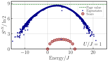
Figure 1: EE as a function of energy. The EE of each state (a blue dot) is given in the unit of $\ln 2$, and its largest value almost saturates at the Page value [68] $S^{\rm Page}=(\ln 3)L/2-1/2$ [58, 59] (a green dashed line). We consider the system size $L=12$ under open boundary conditions and the interaction strength $U/J=1$ in Eq. (3). The quantum number sector with the particle number $N=L$ (unit filling) and the even parity $\mathcal{I}=+1$ is shown. Each QMBS state (a red circle with a dot) with the particle number $N$ has the energy $UN/2$ and the expectation values $\langle\sum_{i=1}^{L}\hat{n}_{i}\rangle=N$ and $\langle\sum_{i=1}^{L}\hat{n}_{i}^{2}\rangle=2N$. Its half-chain EE at $N=L$, corresponding to a state $|S_{n=L/2}\rangle$, becomes $S^{\rm vN}_{A}\rightarrow[\ln(\pi L/8)+1]/2$ for $L\rightarrow\infty$.

Correspondence between the $S=1$ $XY$ model and the constrained BH model. Let us first present the transformation that we use to study the correspondence between the two models. We utilize the improved Holstein-Primakoff expansion [61, 62, 63, 64, 65] for $S=1$ spin operators

$$\hat{S}^{+}_{i}=\sqrt{2}\hat{b}_{i}+(1-\sqrt{2})\hat{b}^{\dagger}_{i}\hat{b}_{i}^{2}+\left(\frac{1}{\sqrt{2}}-1\right)(\hat{b}^{\dagger}_{i})^{2}\hat{b}_{i}^{3},$$ (9)

with $\hat{b}_{i}$ being the boson annihilation operator before the Hilbert space truncation. The advantage over the conventional Holstein-Primakoff expansion is that the Hilbert space on which the operator acts splits into the physical ($n_{i}=0$, $1$, …, $n_{\rm max}=2$) and unphysical ($n_{i}=n_{\rm max}+1$, $n_{\rm max}+2$, …) spaces [66]. Therefore, as long as the operator acts on the state in the physical subspace, the generated states remain physical. The transformation within the physical subspace does not change the spectra of eigenenergies. Consequently, the bosonic operators with the truncated Hilbert space $n_{\rm max}=2$ (namely, $\hat{a}_{i}=\hat{P}_{n_{\rm max}=2}\hat{b}_{i}\hat{P}_{n_{\rm max}=2}$) can be mapped exactly to $S=1$ spin operators. Then, the spin ladder operator $\hat{K}^{+}=\frac{1}{2}\sum_{i}(-1)^{r_{i}}(\hat{S}^{+}_{i})^{2},$ which is used for constructing the QMBS states in the $S=1$ $XY$ model [58, 59], is evaluated as

$$\hat{K}^{+} =\frac{1}{2}\sum_{i}(-1)^{r_{i}}\biggl{[}\sqrt{2}b_{i}^{2}-\sqrt{2}\hat{b}^{\dagger}_{i}\hat{b}_{i}^{3}+\frac{1}{\sqrt{2}}(\hat{b}^{\dagger}_{i})^{2}\hat{b}_{i}^{4}$$

$$~{}\phantom{=}~{}+\left(5-3\sqrt{2}\right)(\hat{b}^{\dagger}_{i})^{3}\hat{b}_{i}^{5}+\left(\frac{3}{2}-\sqrt{2}\right)(\hat{b}^{\dagger}_{i})^{4}\hat{b}_{i}^{6}\biggr{]}.$$ (10)

We immediately see $\hat{K}^{+}\rightarrow\hat{J}^{+}$ with a three-body constraint ($\hat{a}_{i}^{3}=\hat{P}_{n_{\rm max}=2}\hat{b}_{i}^{3}\hat{P}_{n_{\rm max}=2}=0$), indicating the QMBS states in both systems are equivalent.

We then transform the term $\hat{H}^{XY}_{0}=J_{xy}\sum_{i}(\hat{S}^{x}_{i}\hat{S}^{x}_{i+1}+\hat{S}^{y}_{i}\hat{S}^{y}_{i+1})$ in the $S=1$ $XY$ system into the bosonic one. Expanding it by the bosonic operator $\hat{b}_{i}$, we get correlated hopping terms in addition to the conventional boson hopping term:

$$\hat{H}^{XY}_{0} =J_{xy}\sum_{i}(\hat{b}_{i}\hat{b}^{\dagger}_{i+1}+\mathrm{H.c.})$$

$$~{}\phantom{=}~{}+\left(\frac{1}{\sqrt{2}}-1\right)J_{xy}\sum_{i}(\hat{b}_{i}\hat{b}^{\dagger}_{i+1}\hat{\nu}_{i+1}+\hat{b}_{i+1}\hat{b}^{\dagger}_{i}\hat{\nu}_{i}+\mathrm{H.c.})$$

$$~{}\phantom{==}~{}+\left(\frac{3}{2}-\sqrt{2}\right)J_{xy}\sum_{i}(\hat{\nu}_{i}\hat{b}_{i}\hat{b}^{\dagger}_{i+1}\hat{\nu}_{i+1}+\mathrm{H.c.}).$$ (11)

Here, we drop unphysical higher-order terms, which correspond to those containing $\hat{b}_{i}^{3}$ at the rightmost end. Correlated hoppings are known to play a crucial role in stabilizing the QMBS states [53, 54, 69]. By utilizing the improved Holstein-Primakoff expansion, we successfully show that the correlated hopping terms in our model also possess the same QMBS as in the original constrained BH model [66].

Scars in the strong-coupling limit. Let us discuss how the QMBS states behave in the strong-coupling limit, which will be useful for experimental realization as we will explain later. We consider the strong-coupling limit of the BH model on an open chain with a three-body constraint at unit filling: $\hat{H}=-J\sum_{i=1}^{L-1}(\hat{a}^{\dagger}_{i}\hat{a}_{i+1}+\hat{a}^{\dagger}_{i+1}\hat{a}_{i})+\sum_{i=1}^{L}\Omega_{i}\hat{n}_{i}+\frac{U}{2}\sum_{i=1}^{L}\hat{n}_{i}(\hat{n}_{i}-1)$. Here, $\Omega_{i}$ is the external potential, which is often chosen to be a parabolic one in experiments, and the local Hilbert space is spanned by $\{|0\rangle,|1\rangle,|2\rangle\}$. We derive the effective model in the strong $U/J$ limit for the Hilbert subspace satisfying $\sum_{i}n_{i}=N$ (unit filling) and $n_{i}=0$ or $2$ using the Schrieffer-Wolff transformation [70, 71]:

$$\hat{H}_{\mathrm{eff}} =\frac{1}{2}LU+\sum_{i=1}^{L}\Omega_{i}+\frac{1}{2}\sum_{i=1}^{L-1}\tilde{J}_{i,i+1}+\sum_{i=1}^{L}\tilde{h}_{i}\hat{T}_{i}^{z}$$

$$~{}\phantom{=}~{}+2\sum_{i=1}^{L-1}\tilde{J}_{i,i+1}(\hat{T}_{i}^{x}\hat{T}_{i+1}^{x}+\hat{T}_{i}^{y}\hat{T}_{i+1}^{y}-\hat{T}_{i}^{z}\hat{T}_{i+1}^{z}).$$ (12)

Here, we define

$$\tilde{h}_{i} :=2\Omega_{i}-(J_{i,i+1}^{+}-J_{i,i+1}^{-})+(J_{i-1,i}^{+}-J_{i-1,i}^{-}),$$ (13)

$$\tilde{J}_{i,i+1} :=J_{i,i+1}^{+}+J_{i,i+1}^{-}=\frac{2J^{2}U}{U^{2}-(\Omega_{i+1}-\Omega_{i})^{2}},$$ (14)

$$J_{i,i+1}^{\pm} :=\begin{cases}\frac{J^{2}}{U\pm(\Omega_{i+1}-\Omega_{i})},&i=1,2,\dots,L-1,\\ 0,&i=0,L.\end{cases}$$ (15)

The operators $\hat{T}^{\alpha}$ ($\alpha=x,y,z$) are the $S=1/2$ spin operators that act on the space spanned by $\{|0\rangle,|2\rangle\}$, and satisfy $\hat{T}^{z}=(|2\rangle\langle 2|-|0\rangle\langle 0|)/2$ and $\hat{T}^{+}=|2\rangle\langle 0|$. Note that a similar effective model was derived previously [72, 73, 74, 75] although they are different from the present one which prohibits the hopping process containing $n_{i}>2$.

After performing a spin rotation around the $z$ axis by $\pi$ radians for even sites, the effective model in Eq. (Quantum many-body scars in the Bose-Hubbard model with a three-body constraint) transforms into the ferromagnetic Heisenberg model in the absence of the external potential ($\Omega_{i}=0$). The ground state after the transformation is a trivial ferromagnetic state, which includes a state $|\psi_{\mathrm{GS}}^{\mathrm{FM}}\rangle\propto\hat{P}_{\mathrm{UF}}\bigotimes_{j=1}^{L}\frac{|0_{j}\rangle+|2_{j}\rangle}{\sqrt{2}}$ at unit filling. Here, $\hat{P}_{\mathrm{UF}}$ is a projection onto the space at unit filling ($\sum_{i}n_{i}=L$). Then, the corresponding ground state of the original effective model in Eq. (Quantum many-body scars in the Bose-Hubbard model with a three-body constraint) becomes $|\psi_{\mathrm{GS}}^{\mathrm{AF}}\rangle\propto\hat{P}_{\mathrm{UF}}\bigotimes_{j=1}^{L}\frac{|0_{j}\rangle-(-1)^{j}|2_{j}\rangle}{\sqrt{2}}$, which is equivalent to $|S_{L/2}\rangle$ in Eq. (8). Therefore, the exact ground state of the effective model in the strong-coupling limit is embedded in the spectra of eigenstates of the constrained BH model. Note that the effect of small external potential is found to be negligible [66].

Figure 2: Energy spectra as a function of the interaction strength at unit filling. We consider the Hamiltonian in Eq. (3) without the external potential under open boundary conditions, the system size $L=8$, $10$, and $12$, and the interaction strength $J/U=0.01$, $0.02$, $\dots$, $0.1$. The quantum number sector with the particle number $N=L$ and the parity $\mathcal{I}=(-1)^{{\rm mod}(L,4)/2}$ for $L=8$, $10$, and $12$ is given by largest purple, middle green, and smallest blue dots, respectively. Each QMBS state (a red circle with a dot) with the particle number $N(=L)$ has the energy $UN/2$. The effective subspace exhibiting the highest energy ($\approx UL/2$) and that exhibiting the second highest one ($\approx UL/2-U$) are well separated energetically for $U\gg J$. The QMBS state is found to become the lowest-energy eigenstate in the former subspace for sufficiently strong interaction.

Next, let us consider how the QMBS state behaves in the case of $U/J<\infty$. For $U\gg J$, the energy spectrum is divided into well separated bands, and the eigenstates belonging to each band nearly preserve the number of sites at which the particle number takes the values $n_{i}=0$, $n_{i}=1$, and $n_{i}=2$. In the case of unit filling with a three-body constraint, the highest-energy band (consisting of $L/2$ sites with $n_{i}=0$ and $L/2$ sites with $n_{i}=2$ only) and the second highest-energy band (consisting of $L/2-1$ sites with $n_{i}=0$, $L/2-1$ sites with $n_{i}=2$, and remaining $2$ sites with $n_{i}=1$) are well separated energetically (see Fig. 2). Because the QMBS state is the exact eigenstate of the constrained BH model for any $U$, we can always find the QMBS eigenstate in the band consisting of only $n_{i}=0$ and $n_{i}=2$ sites. Remarkably, we have found that the QMBS state corresponds to the lowest-energy eigenstate in this subspace (the highest-energy band) not only at the strong-coupling limit $J/U=0$ but also for $J/U\leq 0.1$, using the exact diagonalization method for $L\leq 12$ [66].

Preparing scars in ultracold-atom experiments. For a wide parameter region of $U\gg J$, the QMBS state is found to become the lowest-energy eigenstate in the highest-energy band, where the particle number takes only the values $0$ and $2$. Therefore, it would be possible to achieve QMBS states in the BH model with a three-body constraint in the following manner: (i) Prepare the $202020\cdots$-type charge-density wave (CDW) state with a choice of $\Omega_{i}=\mathrm{const}\times(-1)^{i}$ to join in the effective $n_{i}=0,2$ subspace [76]. (ii) Make the external potential nearly uniform ($\Omega_{i}\approx\mathrm{const}$) by adiabatically changing it while keeping $U/J$ sufficiently strong. The quantum adiabatic theorem ensures that the final state approaches the lowest-energy eigenstate (equivalent to $|S_{L/2}\rangle$) in the $n_{i}=0,2$ subspace. (iii) Subsequently reduce the potential depth so that the strength of the interaction becomes comparable to the magnitude of hopping. Note that the ETH breaking may be caused by the fragmentation [75] and the QMBS states for $U\gg J$. To purely observe the effect of the QMBS states, it is desirable to prepare the system with smaller $U$.

Concerning the three-body constraint, strong three-body losses of atoms in optical lattices prohibit more than two particles from occupying a single site because of the continuous quantum Zeno effect, resulting in the Bose-Hubbard model with $n_{\rm max}=2$ [76, 77]. To allow control over the ratio of the three-body-loss term to the two-body interaction term, one can use a broad Feshbach resonance [78, 79, 80]. This procedure enables us to realize the much stronger three-body-loss term than the interaction and hopping terms, while keeping periodic potentials shallow so that the interaction is not so strong. Because our QMBS states in the constrained BH model can be realized for both attractive and repulsive interactions, they would be detected in ultracold atoms with three-body losses in optical lattices.

In such QMBS states with a fixed particle number, most of the physical quantities (such as single-particle correlations [81], density-density correlations [82], and the Rényi EE [83, 84]) exhibit almost no time dependence, which would be observed after a sudden quench in experiments. The logarithmic size dependence of the EE growth would also provide a smoking gun for the existence of the QMBS states.

Conclusions. Motivated by the exact construction of the QMBS states in the $S=1$ $XY$ model, we have provided the equivalent athermal states in the BH model with a three-body constraint. To get insight into the mechanism of realizing the QMBS states in the bosonic system, we transform the spin model into the bosonic model using the improved Holstein-Primakoff transformation [61, 62, 63, 64, 65] that does not mix the physical and unphysical Hilbert spaces and consequently does not change the exact energy spectra. The bosonic model obtained after the transformation is similar to the conventional BH model, but with the additional correlated hopping terms, which also possess the same QMBS states. Based on the fact that the QMBS state corresponds to the lowest-energy eigenstate of the effective model for the strong-coupling limit with the highest-energy sector, we propose the realization of the QMBS states in ultracold-atom systems. Moreover, such a local effective Hamiltonian, which also possesses the QMBS states as its eigenstates, would deepen our understanding of the scar phenomena.

Our findings will stimulate further research on the QMBS states in general BH models without any constraints, which would be realized more easily in experiments of ultracold atoms in optical lattices. The construction of the QMBS states in the general spin $S$ system has been discussed recently [85, 86], and it could be extended to the BH model by utilizing the improved Holstein-Primakoff transformation [61, 62, 63, 64, 65]. These QMBS states do not have to be generated according to the conventional $\rm SU(2)$ algebra [85, 86]. This topic will be left for a subject of future study.