Ensembling Uncertainty Measures
to Improve Safety of Black-Box Classifiers

Abstract

Machine Learning (ML) algorithms that perform classification may predict the wrong class, experiencing misclassifications. It is well-known that misclassifications may have cascading effects on the encompassing system, possibly resulting in critical failures. This paper proposes SPROUT, a Safety wraPper thROugh ensembles of UncertainTy measures, which suspects misclassifications by computing uncertainty measures on the inputs and outputs of a black-box classifier. If a misclassification is detected, SPROUT blocks the propagation of the output of the classifier to the encompassing system. The resulting impact on safety is that SPROUT transforms erratic outputs (misclassifications) into data omission failures, which can be easily managed at the system level. SPROUT has a broad range of applications as it fits binary and multi-class classification, comprising image and tabular datasets. We experimentally show that SPROUT always identifies a huge fraction of the misclassifications of supervised classifiers, and it is able to detect all misclassifications in specific cases. SPROUT implementation contains pre-trained wrappers, it is publicly available and ready to be deployed with minimal effort.

1 Introduction

A typical approach to guarantee safety [40] is to equip a functional component with a detector [30], [33], [36], [37] so to trigger a fail-safe or fail-stop behavior whenever the correct functioning is not guaranteed. At the system level, it is often desirable that safety-critical functions would either i) deliver a correct result or ii) omit outputs i.e., the function should have fail-omission failures only. This makes it easy for the system to timely detect the absence of outputs and react accordingly. Through years, safety monitors or safety wrappers have been applied to different functions with beneficial effects on the non-functional (either safety or security [13], [17]) behavior of the component and the encompassing systems. As a result, methodologies, techniques, and industrial applications of safety monitors were largely applied to different functional components and became solid literature with poor research-wise interest.

However, the last twenty years saw a growing interest in developing functional components that (partially) rely on Machine Learning (ML) algorithms that perform classification (classifiers in the paper). Classifiers can model one or more expected behaviors of a system or component and detect deviations that may be due to the occurrence of faults or attacks, and perform error detection, intrusion detection, failure prediction, or out-of-distribution detection [4], [19], [34], to name a few. Straightforwardly, academia, industry, and also National governments hugely invested in methodologies, mechanisms, and tools to embed classifiers into ICT systems, including safety-critical ones. However, classifiers may predict a wrong class for a given data point, which is typically called a misclassification. This is a well-known limitation to the adoption of classifiers to operate safety-critical functions, requiring countermeasures that avoid or mitigate the potential cascading effects of misclassifications to the encompassing system. A fail-omission classifier would either produce trusted outputs or omit them [30]. Clearly, this approach is different from building a classifier that never outputs misclassifications, which is unrealistic to assess at the state of the art due to the dimension of the input space and the unpredictable behavior with inputs close to the decision boundaries [34].

This paper uses uncertainty measures that quantify the confidence in the classification to craft a safety wrapper for black-box classifiers. Uncertainty measures [2], [10], [12], [35] analyze inputs and/or predictions of the classifier and provide a quantitative confidence evaluation. Their goal is to quantify the uncertainty of the classifier’s predictions such that there is significantly different uncertainty between i) the predictions that turn out to be correct, and ii) those that turn out to be misclassifications. In case of high uncertainty, the wrapper should omit the output. We convey the observations above to design, implement and evaluate a Safety wraPper thROugh ensembles of UncertainTy measures (SPROUT). SPROUT wraps a classifier, computes different uncertainty measures, and produces a binary confidence score to suspect misclassifications and decide whether the prediction can be safely propagated to the encompassing system, or if it should be omitted. It can be widely applied because the wrapped classifier is seen as a black-box: internal details do not need to be disclosed.

More in detail, this paper summarizes techniques to compute the uncertainty in the predictions of classifiers, and considers a total of 9 uncertainty measures that can be instantiated with different parameters’ values depending on the needs of the user. These allow to introduce the novel contributions of the paper, which we summarize in three items:

• discuss the application of safety wrappers (or safety monitors) to complement classifiers, converting misclassifications into omissions, and the implications it has in the overall classification process and for the encompassing system;

• describe our Safety wraPper thROugh ensembles of UncertainTy measures (SPROUT) for black-box classifiers, which builds upon the discussion above. SPROUT is easy to use, adapts to any classifier, is publicly available at [5] and available as PIP package;

• show how SPROUT is capable of detecting a huge fraction of the misclassifications of supervised classifiers, even omitting all misclassifications in specific cases.

The paper is organized as follows. Section 2 reviews safety wrappers and the impact they have on failure modes of critical systems. Section 3 describes uncertainty measures, allowing Section 4 to design SPROUT. Section 5 shows how to implement and exercise SPROUT. Section 6 discusses the preliminary assessment, letting Section 7 list threats to validity, and Section 8 concludes the paper.

2 Safety Wrappers for Machine Learning

2.1 On Misclassifications of Machine Learners

Decades of research and practice on ML provided us with plenty of classifiers that are meant to always output a prediction. Supervised classifiers [4], [15], [20], and particularly Deep Learners [8], [9] were proven to achieve excellent classification performance in many domains: they learn their model using data points collected i) during normal operation of the system, and ii) when errors, attacks or failures activate; those data points are then labelled accordingly.

More formally, a classifier clf first devises a mathematical model from a training dataset [4], which contains a given amount of data points. Each data point dp contains a set of f feature values, where each feature value is an image pixel / channel or a floating point number dp_j with $0\leq j<f$ and describes a specific input of the classification problem. Once the model is learned, it can be used to predict the label dp_label of a new data point, different from those in the training dataset. The classification performance is usually computed by applying clf to data points in a test dataset and computing metrics such as accuracy [31], i.e., the percentage of correct predictions of a classifier clf over all predictions. Noticeably, 1 - accuracy quantifies the misclassification probability by difference.

2.2 Failure Modes of Classifiers and Safety Wrappers

Table 1: Probabilities $\alpha_{w}$, $\epsilon_{w}$, $\phi_{c}$, $\phi_{m}$ for outputs of SW(clf) and compound probabilities.

clf behavior $\rightarrow$	Correct Classification	Mislassification	Sum
SW(clf) behavior $\downarrow$
Not Omitted	$\alpha_{w}$	$\epsilon_{w}$	$1-\phi$
Omitted	$\phi_{c}$	$\phi_{m}$	$\phi$
Sum	$\alpha$	$\epsilon$	1

Classifiers are typically meant to provide a best-effort prediction of the class of input data according to the information they have, i.e., the input data and its features. As a result, classifiers sometimes “bet” on a prediction they are unsure of: in these cases, their accuracy may drop significantly. It turns out evident that this best-effort behavior does not pair well with safety-critical systems, which require guarantees of component and system-level behaviors.

It would be beneficial to change the failure semantics of classifiers from uncontrolled content failures (i.e., misclassifications) to omission failures. Fail-controlled components [40] often rely on safety wrappers or monitors [13], [17], [30]. Safety wrappers are intended to complement an existing critical component or task by continuously checking invariants, or processing additional data to detect dangerous behaviors and block the erroneous output of the component before it is propagated through the system. Safety wrappers for classifiers should perform runtime monitoring and aim at detecting the misclassifications of the classifier itself. Regardless of how it is implemented, a safety wrapper SW(clf) transforms a classifier clf which has $0\leq\alpha\leq 1$ accuracy and a misclassification probability $0\leq\epsilon=(1-\alpha)\leq 1$, into a component that has:

• accuracy $\alpha_{w}\leq\alpha$;

• omission probability $0\leq\phi\leq 1$. The SW(clf) may omit misclassifications ($\phi_{m}$, desirable and to be maximized), or correct predictions ($\phi_{c}$, to be minimized). Overall, $\phi=\phi_{m}+\phi_{c}$, and $\alpha_{w}=\alpha-\phi_{c}$;

• residual misclassification probability $\epsilon_{w}$, $0\leq\epsilon_{w}\leq\epsilon\leq 1$; overall, $\epsilon_{w}=\epsilon-\phi_{m}$.

All those probabilities are sketched in Table 2. Ideally, SW(clf) has almost the same accuracy as clf (i.e., $\alpha_{w}\approx\alpha$, or $\phi_{c}\approx 0$), a substantially lower residual misclassification probability, $0\approx\epsilon_{w}<<\epsilon$, and an omission probability close to $\epsilon$ thus $\phi\approx\epsilon$. A SW(clf) will never have better accuracy than clf; however, it will transform most of the misclassifications, which are hardly predictable, detectable and manageable, into omissions.

2.3 Related Work and Motivation

Recently, there have been few studies that specifically aim at building safety wrappers for classifiers [3], [33], [36], [37]. The paper [3] ran a k-nearest neighbor classifier in parallel to a Deep Neural Network (DNN) to detect misclassifications. The paper [33] conducted an active monitoring of the behavior and the operational context of the data-driven system based on distance measures of the Empirical Cumulative Distribution Function, and used them as triggers for the safety wrapper. The work [36] used probabilistic neural networks to model predictive distributions and thus estimate misclassifications thanks to adversarial training. This technique performed well for image classifiers. Lastly, [37] proposed a lightweight monitoring architecture to enhance the model robustness against different unsafe inputs, especially those due to adversarial attacks to neural networks. The logic to detect misclassifications revolved around an analysis of activation patterns of neurons in the layers of a specific neural network, which authors showed to be distinguishable in case of an adversarial input. It is worth mentioning that existing safety wrappers above are classifier-specific (i.e., [3], [10], [37]), often rely on extensive knowledge of the classifier (e.g., [37] requires the structure of the DNN to be disclosed), require the implementation of complex and multi-step processes [33], or apply only to specific types of input data (e.g., [12], [36] are specifically crafted for image classifiers). Instead, we seek for an approach which i) applies to any classifier, which is seen as a black-box; ii) is easy to automatize, adopt and exercise to novel datasets or systems; iii) applies to binary and multi-class classification problems, and iv) does not have any constraint on the input data and as such works with tabular and image datasets.

3 Uncertainty Measures for Classifiers

This section summarizes uncertainty measures that were previously applied to compute the confidence in the prediction of classifiers.

Table 2: Summary of Uncertainty Measures used in this study

UM #	Name of the Uncertainty Measure	Needs Offline Setup	Uses Input Data	Uses Classifier Output	Uses Classifier	Parameters of the Measure
UM1	Confidence Intervals					w: confidence level
UM2	Maximum Likelihood					-
UM3	Entropy of Probabilities					-
UM4	Bayesian Uncertainty					-
UM5	Combined Uncertainty					chk_c: classifier to check agreement with
UM6	MultiCombined Uncertainty					CC: classifiers to check agreement with
UM7	Feature Bagging					bagC: classifier to build bagger set
UM8	Neighbourhood Agreement					k: number of relevant neighbors
UM9	Reconstruction Loss					layers: structure of the AutoEncoder

3.1 Related Works on Uncertainty Measures and their Limitations

Research usually aims at minimizing the probability of misclassifications, thus maximizing accuracy. However, trusting each individual prediction of a classifier, to the extent that the prediction can be propagated towards the encompassing system and used in a (safety-)critical task, is a different problem that is still open [12]. Researchers and practitioners are actively investigating ways to understand if classifiers’ predictions are correct, or if they are misclassifications. The most relevant research results on uncertainty measures are very recent (the last 5 years), which demonstrates the recent emergence and timeliness of the topic. Uncertainty is often [38] referred to as a combination of aleatoric and epistemic uncertainty. The former refers to the notion of randomness, that is, the variability in the outcome of an experiment which is due to inherently random effects e.g., coin-flip. The latter describes uncertainty due to a lack of knowledge of any underlying random phenomenon. In other words, epistemic uncertainty refers to the reducible part of the (total) uncertainty, whereas aleatoric uncertainty refers to the irreducible part [38]. Uncertainty measures quantify the epistemic uncertainty, and can hardly provide useful information to estimate aleatoric uncertainty.

Uncertainty can be statistically estimated through confidence intervals [1] or using the Bayes theorem [2]. Works as [11] estimate uncertainty by using ensembles of neural networks: scores from the ensembles are combined in a unified measure that describes the agreement of predictions and quantifies uncertainty. In [10], [18], authors processed softmax probabilities of neural networks to identify misclassified data points. A new proposal came from [12] and [3], where authors paired a k-Nearest Neighbor classifier with a neural network to compute uncertainty. The work [34] computed the cross-entropy on the softmax probabilities of a neural network, and used it to detect out-of-distribution input data that likely misclassified.

Uncertainty measures above compute either classifier-specific or classifier-independent quantities. However, classifier-specific uncertainty may not always be a meaningful indicator of misclassifications since “neural networks which yield a piecewise linear classifier function […] produce almost always high confidence predictions far away from the training data” [32].

3.2 Quantitative Measures to Compute Uncertainty

This work focuses on uncertainty measures that are not classifier-specific, but instead have a generic formulation that pairs well with any classifier, which is seen as a black-box. This allows avoiding classifier-specific uncertainty, which may be misleading [32]. Table 1 summarizes a total of 9 uncertainty measures UM1 to UM9, which process at least one of: i) input data dp, ii) class prediction dp_prob. Importantly, all measures but UM2, UM3 and UM8 require training data for set-up, and all measures but UM2, UM3, UM4 are parametric, meaning that different values of parameters may be employed to craft different instances of the same measure.

UM1: Confidence Interval A confidence interval defines the statistical distribution underlying the value of a feature and thus provides a range, constrained to the parameter $0\leq w\leq 1$, in which feature values are expected to fall. The confidence level $w$ represents the long-run proportion of feature values (at the given confidence level) that theoretically contain the true value of the feature [41]. UM1 measures how many feature values falls inside their confidence interval. The higher the UM1, the more feature values of dp are outside their confidence interval, which indicates high uncertainty in the prediction.

UM2: Maximum Likelihood Given dp_prob produced by a classifier for a given dp, we identify UM2 as the maximum probability of dp_prob. The higher the UM2, the more uncertain the output of the classifier [18].

UM3: Entropy of Probabilities We retrieve the dp_prob produced by a classifier for a given dp and we compute UM3 using db_prob entropy [10]. The higher the UM3, the more uncertain the classifier: a dp_prob array with constant values (i.e., all classes have the same probability) generates the highest UM3 of 1.

UM4: Bayesian Uncertainty This measure uses a Naïve Bayes process to estimate the probability that the input data point dp belongs to each of the possible c classes [2]. Briefly, this process applies Bayes' theorem assuming strong (i.e., naive) independence between the features. As such, UM4 may not apply to many classification problems, especially those dealing with images, where a pixel (feature) clearly depends on its surrounding pixels.

UM5: Combined Uncertainty UM5 uses a classifier chk_c that acts as a checker of the main classifier clf. UM5 has positive sign if clf and chk_c agree on the predicted class, negative otherwise. The absolute value of UM5 is quantified according to the entropy (UM3) in the results of chk_c. UM5 ranges from -1 to 1. UM5 = 1 translates to high confidence that the prediction of clf is correct, UM5 = -1 means high confidence that the prediction is a misclassification, letting UM5 = 0 show maximum uncertainty.

UM6: Multi-Combined Uncertainty UM6 computes uncertainty relying on more than one checker. UM6 uses a set CC of ncc checking classifiers, computes UM5 for each $chk_{c}\in CC$ with respect to clf, and averages the results. The more checking classifiers in CC agree with clf, the higher the UM6.

UM7: Feature Bagging UM7 exploits the concept of bagging [16], a method for generating multiple versions of a classifier bagC: each instance of bagC is trained using different subsets of the original training set, and decides using restricted knowledge. Should classifiers predict different classes for a given data point dp, UM7 would have low value and predictions should be treated with high uncertainty.

UM8: Neighbor Agreement UM8 finds the k nearest neighbors [15] of a data point dp. Then, it classifies dp and its k neighbors using clf: the more neighbors are assigned to the same class predicted for dp, the higher the UM8. The lower the value, the more disagreement in classifying neighboring data points to dp. This means that the input data point dp lies in an unstable region of the input space, which translates to high uncertainty (low UM8) in the prediction.

UM9 Reconstruction Loss Reconstruction loss quantifies to what extent the input data point is an unseen, out-of-distribution data point [19], and as such it is likely to generate misclassifications. We compute UM9 through the reconstruction error of autoencoders, which are unsupervised neural networks composed of different layers to learn efficient encodings of the input data. A low UM9 value instead indicates that dp belongs to an expected distribution and as such is likely to be correctly classified.

4 SPROUT: a Safety wraPper thROugh ensembles of UncertainTy measures

This section describes our safety wrapper for black-box classifiers, binary or multiclass, which works with tabular and image data.

4.1 Safety Wrappers for Black-Box Classifiers

Figure 1a depicts a typical classifier: the input data, and the features contained therein, are fed into a classifier clf that predicts a class label dp_label for that specific input data dp. This classification process always outputs a class label that is then provided to the encompassing system, has $\alpha$ accuracy and $\epsilon=1-\alpha$ misclassification probability. In this scenario, all the misclassifications are content failures. Figure 1b still feeds the input data to the classifier, which predicts the class dp_label for an input data dp. However, the adoption of a safety wrapper SW(clf) provides the input data and the class prediction of the clf to a misclassification detector, which outputs a binary confidence score [30] (BCS) to decide if the class prediction is detected to be a misclassification. In this case, the wrapper omits the output (with probability $\phi$); otherwise, the class prediction gets forwarded to the encompassing system, is correct with probability $\alpha_{w}$ and is a misclassification with probability $\epsilon_{w}$. There is still a residual probability $\epsilon_{w}$ of content failure, while $\phi_{m}=\epsilon-\epsilon_{w}$ misclassifications are instead going to be omitted thanks to the safety wrapper. Noticeably, insights of clf do not need to be disclosed for detecting misclassifications: as a result, clf is treated as a black-box classifier.

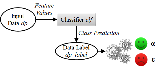
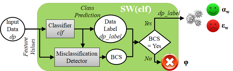
a) Correctly predicts class with $\alpha$ accuracy and $\epsilon=1-\alpha$ misclassification probability

b) Correctly predicts class with $\alpha_{w}$ accuracy, $\phi$ omission probability and $\epsilon_{w}$ residual misclassification probability.

Figure 1: Classifier component (up, Figure 1a) and a classifier inside a safety wrapper (down, Figure 1b).

The existence of a function to generate a dp_label and provide the output probabilities of the classifier is the only assumption we require for wrapping any classifier in such a SW(clf) wrapper. Note that commonly used frameworks for machine learning (to name a few: scikit-learn, xgboost, pyod, tensorflow, pytorch), expose such interfaces; therefore SW(clf) is virtually applicable to any classifier without requiring compliance with restrictive assumptions.

Another important observation regards the applicability of SPROUT to any classifiers, regardless of the domain e.g., image classifiers or classifiers for tabular data, or the specific algorithm to be used, either a DNN, a tree-based classifier, a statistical classifiers, or any other binary or multi-class classifier.

Table 3: Example of uncertainty measures and misclassification flag using a supervised classifier on a specific dataset.

UM1	UM2	UM3	UM4	UM5	UM6_ST	UM6_NB	UM6_TR	UM7	UM8	UM9	Misc flag
0.22	1.00	-0.17	0.47	1.00	1.00	0.90	1.00	0.47	1.00	1.00	correct
0.43	0.39	-0.16	0.57	-0.21	0.40	0.90	0.55	0.57	-0.21	0.4	misc
0.32	0.99	-0.15	-0.41	0.99	0.94	0.69	1.00	-0.41	0.99	0.94	correct

4.2 A Misclassification Detector for SPROUT

The misclassification detector for SPROUT is structured as follows.

SPROUT computes multiple uncertainty measures for each input data and / or the corresponding classifier output: the choice of which uncertainty measures should be computed is of utmost importance [32]. Some uncertainty measures may make SPROUT detect most of the misclassifications (thus the residual misclassification probability $\epsilon_{w}$ would be very low) at a cost of many omissions, i.e., $\phi>>0,\alpha_{w}<<\alpha$. Conversely, other measures may build a SPROUT wrapper that has optimal accuracy ($\alpha_{w}\approx\alpha$, or $\phi_{c}\approx 0$), but rarely omits outputs ($\phi\approx 0$) and fails in detecting many misclassifications ($\epsilon_{w}\approx\epsilon$, or $\phi_{m}\approx 0$) making its behavior similar to the regular clf. We tackle this problem by relying on multiple uncertainty measures amongst those presented in Section 2. Remember that several measures are parameter-dependent and as such can be instantiated multiple times and have a different behavior; this is the case of UM1, UM5, UM6, UM7, UM8 and UM9. The choice of parameters depends on the structure of the input data (e.g., tabular or image data), the type of the classification task (i.e., multi-class or binary) or other specific user needs.

Then, a binary adjudicator processes the ensemble of floating point values computed using each uncertainty measure to output a unique BCS. This binary adjudicator can be implemented with thresholds, invariants, custom rules [14], or as a binary classifier, providing many degrees of freedom in finding the ideal function to combine ensembles of uncertainty measures into a unified BCS, even implementing non-linear decision functions. The resulting misclassification detector will implement a stacking meta-learner, with uncertainty measures at the base level, and a binary adjudicator at the meta-level [60]. Obviously, the classifier that implements each binary adjudicator is decoupled from the classifier clf used for classification.

5 Exercising SPROUT

This section details the experimental campaign to test SPROUT in detecting misclassifications of supervised classifiers.

5.1 Experimental Methodology and its Inputs

As a data baseline, we gather 33 public datasets: 11 datasets (i.e., NSL-KDD [44], ISCX12 [43], UNSW-NB15 [46], UGR16 [50], NGIDS-DS and ADFANet [48], AndMal17 [49], CIDDS-001 [45], CICIDS17 and CICIDS18 [47], SDN20 [51]) of network intrusion detection, datasets of sensor spoofing attacks to 10 different biometric traits summarized in [22] including Fingerprint [52]), Hand Gesture [56]), Electrodermal Activity [54]), Heart Rate [55]), Human Gait [57]), Keystroke [53]), Voice [58]), Face [59]), 7 BackBlaze and BAIDU datasets related to hardware monitoring for failure prediction [24], [25], 3 datasets related to IoT systems (ScaniaTrucks, MechFailure, Iot-IDS ) [27], [26], [28], MNIST and Fashion-MNIST image datasets [6], [7].

We exercise the following 8 supervised classifiers that apply to both tabular and image data, and fit binary and multi-class classification: Decision Tree (DT), Random Forests (RF), eXtreme Gradient Boosting (XGB), Logistic Regression (LR), Naïve Bayes (NB), Linear Discriminant Analysis (LDA), TabNet [8] and FastAI [9] neural networks. The neural networks [8], [9] are explicitly optimized for processing tabular data, which are the majority of our datasets, but pair well also with image datasets. Testing SPROUT with DNNs that are specifically tailored for image classification is something that we will discuss as future work. Regarding the choice of the hyper-parameters for those classifiers, we proceed as follows: we use the HyperOpt [42] library whenever possible (i.e., for all classifiers but FastAI and TabNet). We then let the hyperparameter optimizer that is embedded in FastAI to automatically tune its parameters. For TabNet we ran grid searches with 108 combinations of the following parameters and values: Learning rate $\in[e^{-5},e^{-3},e^{-1}]$, Batch size $\in[512,1024,2048]$, Max Epochs $\in[20,50,100]$, patience (for early stopping) $\in[5,8]$, target metric $\in[mcc,accuracy]$.

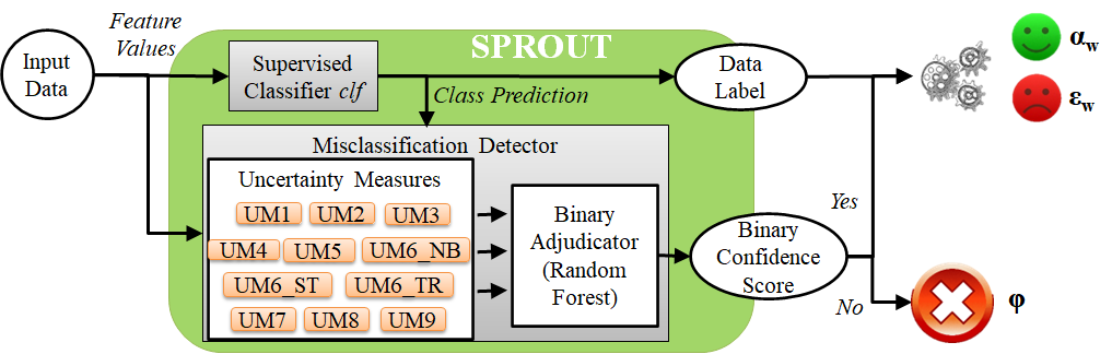
Figure 2: SPROUT wrapper defined and exercised in this paper.

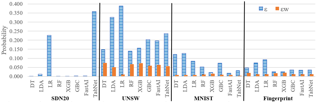
Figure 3: Misclassification probability $\epsilon$ of the classifier (striped bars), and residual misclassification probability $\epsilon_{w}$ (orange bars) of SPROUT for different 8 supervised classifiers exercised on SDN20, UNSW, MNIST and Fingerprint datasets.

We instantiate the following uncertainty measures:

• UM1 with w = 0.9.

• UM2, UM3, and UM4, which do not have parameters.

• UM5 with chk_c = XGB, which is a notoriously good classifier [29].

• UM6 with three different groups of checking classifiers. We indicate the three UM6 configuration as UM6_ST) {NB, LDA, LR}, UM6_TR) {DT, RF, XGB}, and UM6_NB) {GaussianNB, BernoulliNB, MultinomialNB, ComplementNB}. UM6_NB uses variants of the Naïve Bayes (NB) classifier.

• UM7 with bagC = DT, which has low computational complexity and has overall good classification performance. UM7 creates multiple instances of bagC: therefore, a slow bagC would make UM7 take too much time.

• UM8 with k = 19: a prime k avoids ties in kNN searches [15].

• UM9 using 5 layers of the following size: ${f,f/2,f/4,f/2,f}$, being f the number of features in a dataset, which ranges from 4 (ADFANet dataset) to a maximum of 156 (ScaniaTrucks dataset).

Exercising each of the 8 classifiers on each of the 33 datasets and computing uncertainty measures provides a total of 264 csv files that are structured as shown in Table 3.

The reader would notice that we still did not discuss the implementation of the binary adjudicator, which is a classifier and as such needs to be trained itself. Therefore, we split the 264 csv files above into two groups: uncertainty measures (plus the misc flag label) computed for the 8 classifiers on 29 datasets will build the training set of the binary adjudicator, for a total of more than 13 million of labelled data points. The remaining 1.8 million of data points, each containing the uncertainty measures and misc_flag computed for SDN20, UNSW, MNIST, and Fingerprint datasets, will be used as test set for the binary adjudicator and to quantify performance of SPROUT in detecting misclassifications.

We independently exercise Random Forest and XGB classifiers as binary adjudicators, which are known to have excellent classification performance for tabular data [29]: since Random Forests showed better detection accuracy of misclassifications than XGB, we implement the binary adjudicator of SPROUT as a Random Forest composed of 30 trees. This completes the definition and instantiation of SPROUT in Figure 2.

Experiments have been executed on a Dell Precision 5820 Tower with an Intel Xeon Gold 6250, GPU NVIDIA Quadro RTX6000 with 24GB VRAM, 192GB RAM and Ubuntu 18.04, NVIDIA driver 450.119.03 with CUDA 11.0, and required approximately three weeks of 24H execution with GPU support.

5.2 A Library for Exercising SPROUT

SPROUT is available at [5] and as PIP Python package. The package implements all uncertainty measures discussed in this paper and makes SPROUT ready for deployment in any case study. Many already trained models for binary adjudication are already available in the library, and are accompanied by details about the uncertainty calculators they need, statistics on its binary classification performance and on the importance each uncertainty calculator had in learning that model. Those information are not needed to run SPROUT but provide interesting details for explaining why SPROUT works as intended.

Applying SPROUT to a brand new case study is very easy. Below we report a code snippet that shows a simple usage of SPROUT to wrap a supervised classifier from scikit-learn using a pre-defined ($ecai_{s}up$) binary adjudicator which uses the architecture in Figure 2. We assume to have a labeled dataset that we split in two parts. The first part will be provided as input to the $load\_wrapper$ method that prepares a SPROUT wrapper according to the chosen model. Data is used to train the uncertainty measures, while the binary adjudicator is simply loaded from the repository. Then, we initialize and train a RF classifier, which we provide as input, alongside with unlabeled test data, to the $predict\_misclassifications$ function, which outputs i) a pandas DataFrame containing the values of uncertainty measures computed for all the test data points and the associated binary confidence score, and ii) the model of the classifier used for binary adjudication. Binary confidence scores are extracted as numpy array and used to compute $\phi$. If the test set is labeled, we can take advantage of labels to compute $\alpha_{w}$ and $\epsilon_{w}$ as shown in the last rows of Listing 1. Obviously, $y\_te$ labels will not available when deploying SPROUT in a real scenario.

import sklearn as sk, numpy from sprout.SPROUTObject import SPROUTObject # We suppose having a dataset loaded as follows # x: a numpy matrix containing feature values # y: a numpy array containing dataset labels # label_tags: unique labels in y x_tr, x_te, y_tr, y_te = sk.model_selection.train_test_split( x, y, test_size=0.5) # Initializes an empty SPROUT wrapper. so = SPROUTObject() # Loads a specific model for binary adjudication so.load_wrapper(model_tag=’ecai_sup’, x_train=x_tr, y_train=y_tr, la-bel_names=label_tags) # Crafting classifier (can be any) classifier = sk.ensemble.RandomForestClassifier() classifier.fit(x_tr, y_tr) # Suspects misclassifications of clf on test set sp_df, bin_adj = so.predict_misclassifications(data_set=x_te, classifier=classifier) # A numpy array of binary confidence scores sprout_pred = sprout_df[’pred’].to_numpy() phi = 100*numpy.count_nonzero(sprout_pred == 0) / len(sprout_pred) # Computes alpha_w and eps_w # (only if y_test is available) aw = sum((1-sprout_pred)*(1-y_test)) / numpy.count_nonzero(sprout_pred == 0) ew = 1 - phi - aw

6 Results and Discussion

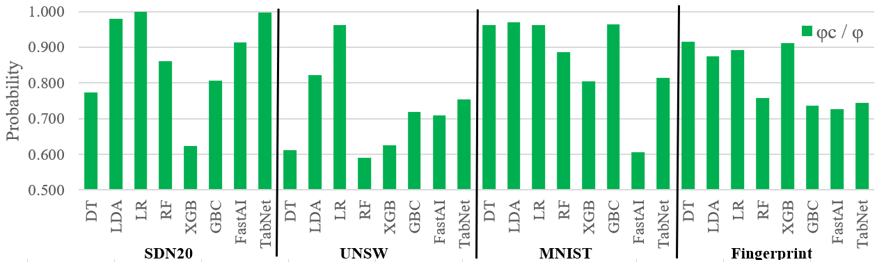
Figure 4: Rate $\phi_{c}/\phi$ of omissions of misclassifications over omissions of SPROUT for different 8 supervised classifiers exercised on SDN20, UNSW, MNIST and Fingerprint datasets.

6.1 Detecting Misclassifications with SPROUT Wrappers

Figure 3 reports a chart that compares the execution of each supervised classifier with respect to its execution inside the SPROUT wrapper: blue striped bars show the misclassification probability $\epsilon$ of clf, while orange solid bars plot the residual misclassification probability $\epsilon_{w}$ of SPROUT. It turns out evident that $\epsilon_{w}$ is always far lower than $\epsilon$ (i.e., orange bars hover on the bottom of the plot and are always lower than 0.1, whereas the blue bars may even reach 0.4), being extremely close to the optimum $\epsilon_{w}\approx 0$ on SDN20 and MNIST datasets. There are cases in which wrapping a clf that has a high misclassification probability $\epsilon$ may yield to the total absence of residual misclassifications $\epsilon_{w}=0$, which is an excellent result. For instance, LR on SDN20 has $\epsilon=0.2263$, meaning that more than 1 out of 5 predictions of clf are misclassifications. Applying the SPROUT wrapper leads to the total absence of residual misclassifications ($\epsilon_{w}=0$), which is an excellent result safety-wise: the output of SPROUT is either a correct misclassification or an omission. As a drawback, SPROUT omits more than 1 out of 5 predictions of the classifier ($\phi=0.2264$), which is not desirable. This high omission probability is a direct consequence of the high $\epsilon$ of LR classifier on SDN20. When the clf to be wrapped has high $\epsilon$ (as it happens in the UNSW dataset), an high omission probability $\phi$ is unavoidable, even when omitting all ($\epsilon_{w}=0$) and only ($\phi_{c}=0$) misclassifications.

On the downside, SPROUT may omit some outputs that were in fact going to be correct classifications. We elaborate more on this aspect with the aid of Figure 4, which plots the ratio of omissions of misclassifications over all omissions i.e., $\phi_{m}/\phi$. The higher the bars in the figure, the higher the $\phi_{m}/\phi$ ratio and the fewer omissions of correct classifications (i.e., $\phi_{c}$ is low). We elaborate more on the case of DT on the UNSW dataset in Figure 4. In this case, only 60% of omissions correspond to misclassifications, which is not desirable: nevertheless, applying SPROUT has still a beneficial impact on residual misclassifications ($\epsilon_{w}=\epsilon/2$), but makes the accuracy $\alpha_{w}$ lower than the baseline ($\alpha=0.852>\alpha_{w}=0.802$). A similar trend can be observed for RF on UNSW and for FastAI on MNIST.

Table 4: Importance of uncertainty measures for binary adjudication (ranked by decreasing importance) and qualitative estimation on time required to compute each measure (H – high, M – medium, L – low, N – no impact, negligible time).

Uncertainty Measure	UM7	UM5	UM6_NB	UM6_ST	UM6_TR	UM3	UM1	UM2	UM9	UM4	UM8
Importance	.289	.189	.138	.128	.128	.036	.032	.027	.017	.010	.004
Time required	M	M	M	M	H	N	L	N	L	L	H

6.2 Importance of Uncertainty Measures

Ultimately, we explore the impact each uncertainty measure has in learning the model for binary adjudication and to detect misclassifications with the aid of Table 4. The first row of the table reports the importance each uncertainty measure (on the columns) has in building the misclassification detector of SPROUT. Those scores are computed through the feature_importances_ of sklearn Python package, and sum up to 1. It turns out evident that some uncertainty measure has marginal contribution for binary adjudication and for detecting misclassifications. Particularly, UM8 has the lowest feature importance and is almost entirely not relevant for detecting misclassifications. Conversely, measures as UM7 and UM5 have the highest importance in building the models for binary adjudication as they carry more information for detecting misclassifications.

We also comment on the time needed to compute each uncertainty measure. Table 4 reports a qualitative estimation for the time needed to compute all uncertainty measures used by SPROUT. Some measures as UM2 and UM3 can be computed in negligible time and do not add any overhead to the classification task. Measures as UM8 and UM6_TR require heavy computations which may significantly slowdown the execution of the classification task. We are aware that the overhead generated by the application of SPROUT may constitute an obstacle in systems which are resource-limited or that have tight real-time deadlines. However, this study primarily aims at building safety wrappers that can detect misclassifications rather than optimizing speed. The reduction of the timing overhead without affecting the other characteristics of SPROUT is discussed as a future work.

7 Threats to Validity and Reproducibility

Internal validity is concerned with factors that may have influenced the results, but they have not been thoroughly considered in the study. First, public datasets are often collected from heterogeneous systems, may have been documented poorly, and are not under our control, but are of utmost importance for enabling reproducibility of this study. Second, classifiers have hyperparameters whose tuning critically affects results: therefore, we exercised sensitivity analyses for the main parameters of all classifiers considered in this study. Third, each classifier may encounter a wide variety of problems when learning a model for each dataset during training (e.g., under/overfitting, poor quality of features, feature selection to leave out noisy features). These events are mostly situational but may have a noticeable impact on the classification performance of a classifier. However, the reader should consider that this paper presents a safety wrapper that detects misclassifications of a black-box classifier, and therefore is not directly impacted by these problems that happened when training the main classifier.

External validity: we cannot claim the validity of this study for classifiers other than those that we used in this study i.e., DNNs for image classification, or unsupervised classifiers. In fact, this analysis is something the we will discuss shortly after as future works. Regarding the application domain of SPROUT, it fits any classification problem, but cannot be generalized easily to regression problems.

The usage of public data and public tools to run algorithms was a prerequisite of our analysis to allow reproducibility and to rely on proven-in-use data. We publicly shared scripts, methodologies and all metric scores, allowing any researcher or practitioner to repeat the experiments. We do not use any custom or private dataset: all dataset are referenced in the papers, and all code is available at [5].

8 Conclusions and Future Works

This paper presented a safety wrapper to detect misclassifications of a black-box classifier. SPROUT, our Safety wraPper thROugh ensembles of UncertainTy measures, creates a wrapper around a classifier, either binary or multi-class, and processes tabular or image input data. SPROUT computes multiple uncertainty measures, providing quantitative data to detect misclassifications of a classifier. Whenever a misclassification is detected, SPROUT blocks the propagation of the output of the classifier to the encompassing system: this way, a content failure of the classifier is transformed into an omission failure, which can be easily handled by the encompassing system. SPROUT wrappers for supervised classifiers are available in the library available at [5]. Results in this paper show that SPROUT correctly detects the large majority of misclassifications of all the classifiers we used, and can even detect all misclassifications of some classifiers (e.g., Logistic Regression on the SDN20 dataset).

We are aware that we may have left out other uncertainty measures and other groups of classifiers (i.e., unsupervised, neural networks for image classification) from this study. Whereas the design and purpose of SPROUT will not be affected by those additional measures and classifiers, they may contribute to a more solid experimental analysis which we plan as future work. In particular, we will craft SPROUT wrappers for unsupervised classifiers and conduct additional experiments that emphasize more on image classification, applying SPROUT to pre-trained deep neural network models from the ImageNet model zoos [39] of pytorch and tensorflow, and processing well-known datasets other than those already considered in this study, e.g., CIFAR-10 and ImageNet. As an additional but not least important future work, we will focus on lowering the timing overhead introduced by SPROUT wrappers with respect to a traditional classification process. Uncertainty measures that individually introduce major overhead will be evaluated to understand if i) they could be dropped without affecting the behavior of wrappers, ii) their implementation could be optimized, or iii) they could be replaced with faster alternatives.

This work was partially supported by project SERICS (PE00000014) under the MUR National Recovery and Resilience Plan funded by the European Union - NextGenerationEU and by the NextGenerationEU program, Italian DM737 – CUP B15F21005410003."

References

1. Meeker, W. Q., Hahn, G. J., & Escobar, L. A. (2017). Statistical intervals: a guide for practitioners and researchers (Vol. 541). John Wiley & Sons.

2. Krzanowski, W. J., et. Al. (2006). Confidence in classification: a bayesian approach. Journal of Classification, 23(2), 199-220.

3. Bilgin, Z., & Gunestas, M. (2021). Explaining Inaccurate Predictions of Models through k-Nearest Neighbors. In ICAART (2) (pp. 228-236).

4. Bishop, C. M. (2006). Pattern recognition. Machine learning, 128(9).

5. SPROUT Repository on GitHub (online), https://github.com/tommyippoz/SPROUT

6. LeCun, Y. (1998). The MNIST database of handwritten digits. (online) http://yann.lecun.com/exdb/mnist/.

7. Fashion-MNIST: a Novel Image Dataset for Benchmarking Machine Learning Algorithms. Han Xiao, Kashif Rasul, Roland Vollgraf. arXiv:1708.07747

8. Arik, S. Ö., & Pfister, T. (2021, May). Tabnet: Attentive interpretable tabular learning. In Proceedings of the AAAI Conference on Artificial Intelligence, Vol. 35 (8), pp. 6679-6687.

9. Howard, J. et. Al. (2020). Fastai: a layered API for deep learning. Information, 11(2), 108.

10. Dan Hendrycks and Kevin Gimpel. A baseline for detecting misclassified and out-of-distribution examples in neural networks. arXiv preprint arXiv:1610.02136, 2016.

11. Lakshminarayanan, et. Al. Safety and scalable predictive uncertainty estimation using deep ensembles. In Advances in Neural Information Processing Systems, pp 6405–6416, 2017.

12. Jiang, H., Kim, B., Guan, M., & Gupta, M. (2018). To trust or not to trust a classifier. Advances in neural information processing systems, 31.

13. Pham, C., Estrada, Z., Cao, P., Kalbarczyk, Z., & Iyer, R. K. (2014, June). Reliability and security monitoring of virtual machines using hardware architectural invariants. In 2014 44^th IEEE/IFIP Int. Conference on Dependable Systems and Networks (pp. 13-24). IEEE.

14. Di Giandomenico, F., & Strigini, L. (1990, October). Adjudicators for diverse-redundant components. Proc. 9^th Symposium on Reliable Distributed Systems (pp. 114-123). IEEE.

15. Cheung, K. L., & Fu, A. W. C. (1998). Enhanced nearest neighbor search on the R-tree. AUM SIGMOD Record, 27(3), 16-21.

16. Breiman, L. (1996). Bagging predictors. Machine learning, 24(2), 123-140.

17. Tiwari, A., Dutertre, B., Jovanović, D., de Candia, T., Lincoln, P. D., Rushby, J., … & Seshia, S. (2014, April). Safety wrapper for security. In Proceedings of the 3^rd international conference on High confidence networked systems (pp. 85-94).

18. Fonseca, J. R., et. al. (2005). Uncertainty identification by the maximum likelihood method. Journal of Sound and Vibration, 288(3), 587-599.

19. Xiao, Z., Yan, Q., & Amit, Y. (2020). Likelihood regret: An out-of-distribution detection score for variational auto-encoder. Advances in neural information processing systems, 33, 20685-20696.

20. Kramer, M. A. (1991). Nonlinear principal component analysis using autoassociative neural networks. AIChE journal, 37(2), 233-243.

21. Nour Moustafa, Jill Slay. 2015. “UNSW-NB15: a comprehensive data set for network intrusion detection systems”. In Military Communications and Information Systems Conference (MilCIS), 2015. IEEE, 1–6.

22. Zoppi, T., Gharib, M., Atif, M., & Bondavalli, A. (2021). Meta-Learning to Improve Unsupervised Intrusion Detection in Cyber-Physical Systems. ACM Transactions on Cyber-Physical Systems (TCPS), 5(4), 1-27.

23. Ring, M., Wunderlich, S., Scheuring, D., Landes, D., & Hotho, A. (2019). A survey of network-based intrusion detection data sets. Computers & Security.

24. BackBlaze: BackBlaze Hard Drive Data (online) https://www.backblaze.com/b2/hard-drive-test-data.html

25. BAIDU: Baidu Smart HDD Competition (online) https://www.kaggle.com/drtycoon/baidu-hdds-dataset-2017/version/1

26. MechFailure: Machine Failure Prediction Competition (online), https://www.kaggle.com/c/machine-failure-prediction

27. Gondek C., e. al. (2016) Prediction of Failures in the Air Pressure System of Scania Trucks Using a Random Forest and Feature Engineering. In Advances in Intelligent Data Analysis XV. IDA 2016. Lecture Notes in Computer Science, vol 9897. Springer, Cham

28. IoT-IDS: IoT Intrusion (online) https://ieee-dataport.org/open-access/iot-network-intrusion-dataset#files

29. Shwartz-Ziv, R., & Armon, A. (2022). Tabular data: Deep learning is not all you need. Information Fusion, 81, 84-90.

30. Guérin, J., Ferreira, R. S., Delmas, K., & Guiochet, J. (2022, October). Unifying evaluation of machine learning safety monitors. In 2022 IEEE 33rd International Symposium on Software Reliability Engineering (ISSRE) (pp. 414-422). IEEE.

31. Lever, J. (2016). Classification evaluation: It is important to understand both what a classification metric expresses and what it hides. Nature methods, 13(8), 603-605.

32. Hein, M., Andriushchenko, M., & Bitterwolf, J. (2019). Why relu networks yield high-confidence predictions far away from the training data and how to mitigate the problem. In Proc. of the IEEE/CVF Conference on Computer Vision and Pattern Recognition (pp. 41-50).

33. Aslansefat, K., et. al. (2020, September). SafeML: safety monitoring of machine learning classifiers through statistical difference measures. In International Symposium on Model-Based Safety and Assessment (pp. 197-211). Springer, Cham.

34. Wang, M., Shao, Y., Lin, H., Hu, W., & Liu, B. (2022). Cmg: A class-mixed generation approach to out-of-distribution detection. Proceedings of ECML/PKDD-2022.

35. Shafaei, S., Kugele, S., Osman, M. H., & Knoll, A. (2018, September). Uncertainty in machine learning: A safety perspective on autonomous driving. In International Conference on Computer Safety, Reliability, and Security (pp. 458-464). Springer, Cham.

36. Lakshminarayanan, B., Pritzel, A., & Blundell, C. (2017). Simple and scalable predictive uncertainty estimation using deep ensembles. Advances in neural information processing systems, 30.

37. Rossolini, G., Biondi, A., & Buttazzo, G. (2022). Increasing the Confidence of Deep Neural Networks by Coverage Analysis. IEEE Transactions on Software Engineering.

38. Hüllermeier, E., & Waegeman, W. (2021). Aleatoric and epistemic uncertainty in machine learning: An introduction to concepts and methods. Machine Learning, 110(3), 457-506.

39. Model Zoo - Discover open source deep learning code and pretrained models (online), https://modelzoo.co/ accessed: 2023-01-20

40. Avizienis, A., Laprie, J. C., Randell, B., & Landwehr, C. (2004). Basic concepts and taxonomy of dependable and secure computing. IEEE transactions on dependable and secure computing, 1(1), 11-33.

41. Hazra, A. (2017). Using the confidence interval confidently. Journal of thoracic disease, 9(10), 4125.

42. Bergstra, J., Komer, B., Eliasmith, C., Yamins, D., & Cox, D. D. (2015). Hyperopt: a python library for model selection and hyperparameter optimization. Computational Science & Discovery, 8(1), 014008.

43. Ali Shiravi, Hadi Shiravi, Mahbod Tavallaee, and Ali A Ghorbani. 2012. Toward developing a systematic approach to generate benchmark datasets for intrusion detection. Computers & Security 31, 3 (2012), 357–374.

44. Mahbod Tavallaee, Ebrahim Bagheri, Wei Lu, and Ali A Ghorbani. 2009. A detailed analysis of the KDD CUP 99 data set. In Computational Intelligence for Security and Defense Applications, 2009. CISDA 2009. IEEE Symposium on. IEEE, 1–6.

45. Ring, M., et. Al. (2017, June). Flow-based benchmark data sets for intrusion detection. In Proceedings of the 16th European Conference on Cyber Warfare and Security. ACPI (pp. 361-369).

46. Nour Moustafa, Jill Slay. 2015. “UNSW-NB15: a comprehensive data set for network intrusion detection systems”. In Military Communications and Information Systems Conference (MilCIS), 2015. IEEE, 1–6.

47. Sharafaldin, I., Lashkari, A. H., & Ghorbani, A. A. (2018, January). Toward Generating a New Intrusion Detection Dataset and Intrusion Traffic Characterization. In ICISSP (pp. 108-116).

48. Haider, W., Hu, J., Slay, J., Turnbull, B. P., & Xie, Y. (2017). Generating realistic intrusion detection system dataset based on fuzzy qualitative modeling. Journal of Network and Computer Applications, 87, 185-192.

49. Lashkari, A. H., et. Al. (2018, October). Toward Developing a Systematic Approach to Generate Benchmark Android Malware Datasets and Classification. In International Carnahan Conference on Security Technology (ICCST) (pp. 1-7). IEEE.

50. Maciá-Fernández, G., Camacho, J., Magán-Carrión, R., García-Teodoro, P., & Theron, R. (2018). UGR ’16: A new dataset for the evaluation of cyclostationarity-based network IDSs. Computers & Security, 73, 411-424.

51. Elsayed, M. S., Le-Khac, N. A., & Jurcut, A. D. (2020). InSDN: A Novel SDN Intrusion Dataset. IEEE Access, 8, 165263-165284.

52. BIT – Biometrics Ideal Test, CASIA-FingerprintV5, http://biometrics.idealtest.org/

53. Adams, Warwick R. “High-accuracy detection of early Parkinson’s Disease using multiple characteristics of finger movement while typing.” PloS one 12.11 (2017): e0188226.

54. Koldijk, S., Sappelli, M., Verberne, S., Neerincx, M. A., & Kraaij, W. (2014, November). The swell knowledge work dataset for stress and user modeling research. In Proceedings of the 16th international conference on multimodal interaction (pp. 291-298).

55. Philip Schmidt, Attila Reiss, Robert Duerichen, Claus Marberger, Kristof Van Laerhoven, “Introducing WESAD, a multimodal dataset for Wearable Stress and Affect Detection”, ICMI 2018, Boulder, USA, 2018

56. A. Memo, L. Minto, P. Zanuttigh, “Exploiting Silhouette Descriptors and Synthetic Data for Hand Gesture Recognition”, STAG: Smart Tools & Apps for Graphics, 2015

57. Vajdi, A., Zaghian, M. R., Farahmand, S., Rastegar, E., Maroofi, K., Jia, S., … & Bayat, A. (2019). Human Gait Database for Normal Walk Collected by Smart Phone Accelerometer. arXiv preprint arXiv:1905.03109.

58. Kaggle – Voice Recognition, Jeganathan Kolappan. https://www.kaggle.com/jeganathan/voice-recognition (online), accessed: 2022-11-20

59. Kaggle – Face Images with Marked Landmark Points, Omri Goldstein. https://www.kaggle.com/drgilermo/face-images-with-marked-landmark-points (online), accessed: 2022-11-20

60. Wolpert, D. H. (1992). Stacked generalization. Neural networks, 5(2), 241-259.