IncreLoRA: Incremental Parameter Allocation Method for
Parameter-Efficient Fine-tuning

Abstract

With the increasing size of pre-trained language models (PLMs), fine-tuning all the parameters in the model is not efficient, especially when there are a large number of downstream tasks, which incur significant training and storage costs. Many parameter-efficient fine-tuning (PEFT) approaches have been proposed, among which, Low-Rank Adaptation (LoRA) is a representative approach that injects trainable rank decomposition matrices into every target module. Yet LoRA ignores the importance of parameters in different modules. To address this problem, many works have been proposed to prune the parameters of LoRA. However, under limited training conditions, the upper bound of the rank of the pruned parameter matrix is still affected by the preset values. We, therefore, propose IncreLoRA, an incremental parameter allocation method that adaptively adds trainable parameters during training based on the importance scores of each module. This approach is different from the pruning method as it is not limited by the initial number of training parameters, and each parameter matrix has a higher rank upper bound for the same training overhead. We conduct extensive experiments on GLUE to demonstrate the effectiveness of IncreLoRA. The results show that our method owns higher parameter efficiency, especially when under the low-resource settings where our method significantly outperforms the baselines. Our code is publicly available.

1 Introduction

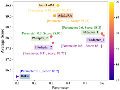
Figure 1: Fine-tuning results for different methods and parameter budget on the GLUE benchmark, all experiments are based on DeBERTaV3-base. We compare our method with BitFit (Zaken, Goldberg, and Ravfogel 2022), PAdapter (Pfeiffer et al. 2021), HAdapter (Houlsby et al. 2019a), and AdaLoRA (Hu et al. 2022), with the x-axis representing the number of parameters (M), and the y-axis representing the average score (Avg). Our approach achieves a better trade-off between efficiency and performance.

In recent years, pre-training models with large amounts of data and fine-tuning them for different downstream tasks have become one of the most successful training paradigms (Peters et al. 2018; Devlin et al. 2019; Radford et al. 2018; Liu et al. 2019; Radford et al. 2021; Raffel et al. 2020). However, with the increasing size of popular pre-trained models, such as BERT (110M$\sim$340M) (Devlin et al. 2019), T5 (60M$\sim$11B) (Raffel et al. 2020) , GPT3 (175B) (Brown et al. 2020), LLaMA (7B$\sim$65B) (Touvron et al. 2023), it becomes difficult to train these models due to graphics card memory limitations, and it is expensive to train and store the full parameters of the model for each downstream task.

Parameter-Efficient Fine-Tuning (PEFT) is a promising solution to the above problems. As the name implies, parameter-efficient fine-tuning achieves performance comparable to full parametric fine-tuning by making only a small number of parameter changes to the model. Due to its broad application prospects, researchers have proposed various methods for efficient parameter tuning (Houlsby et al. 2019a; Lester, Al-Rfou, and Constant 2021a; Li and Liang 2021; Zaken, Goldberg, and Ravfogel 2022; Hu et al. 2022). Some methods only fine-tune part of the parameters of the original model (Guo, Rush, and Kim 2021a; Zaken, Goldberg, and Ravfogel 2022), while others train a batch of new parameters and add them to the original model (Houlsby et al. 2019a; Pfeiffer et al. 2021; Sung, Cho, and Bansal 2022). LoRA (Hu et al. 2022) is one of the representative methods, which simulates a low-rank update matrix $\Delta W$ of the same size as the original weight matrix through the product of two low-rank matrices, and updates only two low-rank matrices during the fine-tuning process (usually only $0.01\%-0.5\%$ of the original matrix parameter count, depending on the rank of the matrices), but achieves a full update of the original weight matrix. Despite the low-rank parameter update $\Delta W$, experimental results show that the fine-tuning performance of LoRA approaches or exceeds that of full fine-tuning (Hu et al. 2022).

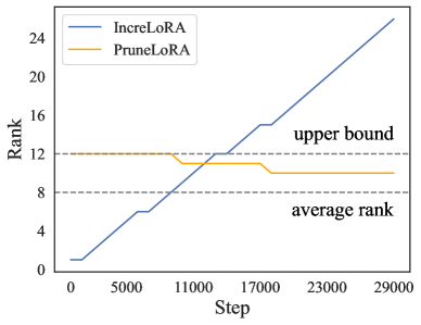
Figure 2: We illustrate the variations in rank of layer.10.attention.self.value_proj when fine-tuning DeBERTaV3-base on MNLI, using IncreLoRA and Pruning LoRA methods respectively.

LoRA has been introduced to various tasks (Dettmers et al. 2023; Lawton et al. 2023; Smith et al. 2023) due to its simple structure, but it sets the same rank for each update matrix equally, ignoring the differences between modules, and it has been demonstrated that assigning different ranks to different update matrices achieves better fine-tuning performance for the same total number of trainable parameters (Zhang et al. 2023; Lawton et al. 2023). This type of method can be recognized as a pruning of the LoRA method, although better performance has been achieved, however, the rank of each LoRA module is still limited by the rank before pruning (The module rank here actually refers to the rank of the update matrix obtained from the product of two low-rank matrices in the module, in the following, we will use both terms). The aforementioned structured pruning methods typically set the initial average rank to be 1.5 times that of the final state. For instance, if the average rank after pruning is 8, then the initial rank for each module would be 12. As illustrated in Figure 2, the rank of unimportant modules will decrease (potentially to 0, meaning no parameter updates) after the pruning process, and more important modules have a rank that is most likely greater than 8, but still cannot exceed the initial upper bound of rank=12. In order to make each module have a higher upper bound on the rank after pruning, it is necessary to set each module with a higher initial rank, which will undoubtedly raise the training cost of the model and require more iterations to make the training stable.

To resolve the above contradiction, we propose IncreLoRA, an incremental trainable parameter allocation method, which automatically increases the rank based on the importance score of each module during the training process, and each module has a higher rank upper bound at the same training cost. In order to prevent insufficient training of subsequently added parameters, we use a new pre-training technique to allow the parameters added to the module to have a favorable initial state, which we call advance learning to show the difference. Moreover, we assign independent learning rate curves to these parameters to ensure the stability of training. As shown in Figure 1, our experimental results show that our proposed method achieves better performance, especially in the low-resource case, and our method performs well enough to match other methods with higher parameter budgets. The contributions of this paper are summarized as follows:

• We propose IncreLoRA which has a lower training cost and higher rank upper bound in comparison to pruning methods. To the best of our knowledge, it is the first parameter-efficient fine-tuning method that incrementally assigns trainable parameters.

• We introduce a new parameter pre-training method, which allows the parameters to find a better state in advance while ensuring training stability and without taking up additional training time.

• We conduct extensive experiments on natural language understanding benchmark, and the results demonstrate the effectiveness of the model we introduce.

2 Related Work

As a method to reduce the cost of fine-tuning and storage of large-scale pre-trained models, PEFT has received more and more attention from researchers in recent years, with different methods varying in terms of memory efficiency, storage efficiency, and inference overhead. According to whether the original parameters are fine-tuned in the training phase, existing PEFT methods can be categorized into selective and additive.

2.1 Selective Method

Selective Methods pick and update the model based on its original parameters. Fine-tuning only a few top layers of the network (Donahue et al. 2014) can be seen as an early attempt at PEFT, while many methods proposed in recent years select specific model layers (Gheini, Ren, and May 2021) or internal modules, e.g., BitFit (Zaken, Goldberg, and Ravfogel 2022) updates only the bias parameters in the model, which dramatically reduces the number of trainable parameters, but this brute-force approach can only lead to sub-optimal performance. Unstructured parameter fine-tuning based on the scoring function in parameter selection of trainable parameters (Vucetic et al. 2022; Sung, Nair, and Raffel 2021a; Ansell et al. 2022; Guo, Rush, and Kim 2021b) is a more complete solution. FishMask (Sung, Nair, and Raffel 2021b) performs multiple iterations on the sub-data according to the model and calculates the amount of parameter Fisher information, and then constructs a mask to select the $k$ parameters with the maximum Fisher information for updating. However, since existing deep learning frameworks and hardware cannot well support the computation of such unstructured sparse matrices, it has a similar memory footprint during training and full parameter fine-tuning.

2.2 Additive Method

The Additive Method replaces full-parameter fine-tuning by adding trainable additional parameters to the prototype network, Adapters are trainable mini-modules inserted into the original network, which were first applied to multi-domain image categorization (Rebuffi, Bilen, and Vedaldi 2017), and later introduced after Transformer’s Attention and FNN layers (Houlsby et al. 2019b), and have given rise to many variants (Mahabadi, Henderson, and Ruder 2021; Wang et al. 2022; He et al. 2022b). Unlike methods like Adapters, LoRA (Hu et al. 2022) simulates the update of the weight matrix in the model by the product of two low-rank matrices, and the trained parameters can be added to those in the original network during the inference phase without incurring additional inference overhead. Prefix-Tuning (Li and Liang 2021) adds the trainable parameters before the sequence of hidden states in all layers. A similar approach is Prompt-Tuning (Lester, Al-Rfou, and Constant 2021b). LST (Sung, Cho, and Bansal 2022) feeds hidden states from the original network into a small trainable ladder side network via shortcut connections, so that the gradients do not need to be backpropagated through the backbone network, further reducing the memory utilization.

2.3 Hybrid Method

Based on the impressive performance of PEFT methods mentioned above, many works have focused on mining the effectiveness of different methods and designing unified frameworks to combine them for optimal performance (Mao et al. 2022; He et al. 2022a; Chen et al. 2023), however, they still belong to the early manual attempts. Recently, many works have been based on the idea that the parameter redundancy has also existed in PEFT modules, pruning the trainable parameters to achieve better fine-tuning performance with a limited parameter budget (Bai et al. 2022; Zeng, Zhang, and Lu 2023; Lawton et al. 2023). Lawton et al. (2023) applies both structured and unstructured methods for pruning LoRA. Zeng, Zhang, and Lu (2023) lets all layers share the same single PEFT module (e.g., Adapter, LoRA, and Prefix-Tuning) and learns a binary mask for each layer to select different sub-networks.

3 Methodology

The idea of our approach is the gradual increase of the trainable parameters of the model during the training process. Based on our observations, incremental parameter allocation without any improvement strategies is likely to result in training insufficiency and instability, thereby leading to poor fine-tuning performance. Note that we focus on how to improve this particular training approach instead of proposing a new importance scoring function. For this Section, we first present how we reconstruct the low-rank matrices in LoRA in Section 3.1, then present the details of the parameter allocation strategy in Section 3.2, and eventually describe how to utilize the reconstructed low-rank matrices for advance learning in Section 3.3.

3.1 Reconstructing Low-Rank Matrices

For a pre-trained weight matrix $W^{\left(0\right)}\in\mathbb{R}^{out\times in}$, we define the parameter efficient fine-tuning as an update matrix $\Delta W$. LoRA (Hu et al. 2022) decomposes it into the product of two low-rank matrices:

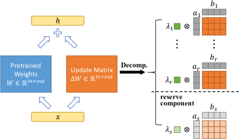
Figure 3: An illustration of the low-rank adapters in our model, where $x$ is the input of each module and $h$ is the output of the module. The update matrix $\Delta W$ can be decomposed into $r$ components and an additional preparatory component. where $\lambda_{s}$ is fixed to 1e-5 and the remaining parameters are trainable.

$$W=W^{\left(0\right)}+\Delta W=W^{\left(0\right)}+BA,$$ (1)

where $A\in\mathbb{R}^{r\times in},B\in\mathbb{R}^{out\times r}$ and the rank $r\ll\min\left(in,out\right)$. A scaling factor is also applied to this update matrix, usually set to $1/r$. $A$ and $B$ can be viewed as a combination of a set of vectors: $A=\left[a_{1},a_{2},\cdots,a_{r}\right],B=\left[b_{1},b_{2},\cdots,b_{r}\right]$, where $a_{i}\in\mathbb{R}^{in},b_{i}\in\mathbb{R}^{out}$. Thus equation (1) can be further disassembled as:

$$\begin{split}W&=W^{\left(0\right)}+w_{1}+w_{2}+\cdots+w_{r}\\ &=W^{\left(0\right)}+b_{1}a_{1}+b_{2}a_{2}+\cdots+b_{r}a_{r},\end{split}$$ (2)

where $w_{i}$ is a matrix of rank 1 obtained by the product of the vectors $b_{i},a_{i}$ .

To match our proposed advance learning strategy, we add a scaling $\lambda_{i}$ to each $w_{i}$, so equation (1) is updated into:

$$W=W^{\left(0\right)}+\sum_{i=1}^{r}{\lambda_{i}w_{i}}=W^{\left(0\right)}+\sum_{i=1}^{r}{\lambda_{i}b_{i}a_{i}},$$ (3)

where $\lambda_{i}$ is updated through backpropagation. We apply random Gaussian initialization to each $a_{i}$ and $b_{i}$, while $\lambda_{i}$ is initialized to zero to ensure that the initial state of $\Delta W$ is zero. In order to reduce the dependency between $w_{i}$ and to ensure the stability of training, we apply a regularization term which is introduced by Zhang et al. (2023):

$$R\left(A,B\right)=\lVert A^{T}A-I\rVert_{\text{F}}^{2}+\lVert B^{T}B-I\rVert_{\text{F}}^{2},$$ (4)

where $I$ is an identity matrix, this forces $A$ and $B$ to be orthogonal after training, and the Frobenius norm of the trained $w_{i}$ equal to one, and the effect of each $w_{i}$ on $\Delta W$ controlled by $\lambda_{i}$. Let $\Lambda=\left[\lambda_{1},\lambda_{2},\cdots,\lambda_{r}\right]$, then $\Delta W=B\Lambda A$, which is similar in form to the singular value decomposition (SVD), except that $\lambda_{i}$ can be an arbitrary constant, whereas the singular values in the SVD are non-negative. In our model, we replace the original LoRA matrix with a SVD-like triplets, and since $\Lambda$ is a diagonal matrix, we can store it with only a one-dimensional tensor, which introduces only $r$ additional parameters for each module.

In the training of common transformer-base models, LoRA is typically appended to the key and value projection matrices in the attention layer. In our approach, however, parameter updates are applied to all linear layers, with the update matrix ranks being scheduled by a allocator according to importance scores.

3.2 Incremental Parameter Allocation

Unlike the pruning approach, the amount of trainable parameters for our model increases with training. We utilize rank to denote the parameter budget for each module, and the sum of all ranks at the end of training, denoted as $r^{final}$, represents the total number of ranks we can assign. At model initialization, the rank of each module is one. During the parameter allocation phase, the total rank of the model, $r^{total}$, increases linearly until the end of parameter allocation, when $r^{total}$ equals $r^{final}$.

At the t$-th$ step of the phase, an importance score $S^{\left(t\right)}_{k}$ needs to be maintained for each module, for $k=1,2,...,n$, where $k$ is the index of the module and $n$ is the total number of modules. We make $S^{\left(t\right)}_{k}$ equal to the average of the scores of all parameters of the update matrix (Molchanov et al. 2019):

$$S^{\left(t\right)}_{k}=avg\left(\left|\Delta W_{k}*grad\left(\Delta W_{k}\right)\right|\right).$$ (5)

The update matrix is modeled by the product of $B$, $\Lambda$ and $A$, we can can capture the gradient when backpropagating to this matrix via a backward hook. Since we take mini-batch training, the score of each step is affected by the randomness of sampling, so we improve the reliability of the score by sensitivity smoothing and uncertainty quantification (Zhang et al. 2022):

$$I_{k}^{\left(t\right)} =\beta_{1}I_{k}^{\left(t-1\right)}+\left(1-\beta_{1}\right)S_{k}^{\left(t\right)},$$ (6)

$$U_{k}^{\left(t\right)} =\beta_{2}U_{k}^{\left(t-1\right)}+\left(1-\beta_{2}\right)\left|I_{k}^{\left(t\right)}-S_{k}^{\left(t\right)}\right|,$$ (7)

$$\hat{S}_{k}^{\left(t\right)} =I_{k}^{\left(t\right)}*U_{k}^{\left(t\right)},$$ (8)

where $0<\beta_{1},\beta_{2}<1$. $\hat{S}_{k}^{\left(t\right)}$ is the importance score we actually utilize. At intervals of $\nu$ steps, the allocator adds a new set of parameters for all modules with scores in the top-$h$, where $\nu$ and $h$ are hyperparameters, we default $\nu$ to equal warmup steps. Theoretically, at the start of each training session, the upper bound of rank for each module is $r^{final}/h$.

Algorithm 1 IncreLoRA. $\mathcal{D}$ is dataset, $\mathcal{M}$ is target module set, $\mathcal{A},\mathcal{B},\mathcal{E}$ is the set of parameter matrices, $T$ is total steps, $\mathcal{W}$ is warmup steps, $\eta$ is learning rate, $h$ is the number of modules selected in each round, $r^{final}$ is final total rank.

Input:$\mathcal{D}$, $T$, $\mathcal{W}$, $\eta$, $h$, $r^{final}$
Parameter: $\mathcal{A},\mathcal{B},\mathcal{E}$

1:  for $M_{k}$ in $\mathcal{M}$ do

2:     Append $a_{k},b_{k},\lambda_{k}$ to $A_{k}^{\left(0\right)},B_{k}^{\left(0\right)},\Lambda_{k}^{\left(0\right)}$ for advance learning

3:     init_normal$\left(a_{k},b_{k}\right)$; freezed$\left(\lambda_{k}\right)\leftarrow 1e-5$

4:  end for

5:  for $t=1,...,T$ do

6:     if $r^{total}<r^{final}$ then

7:        Compute $\hat{S}_{k}^{\left(t\right)}$ by (5),(6),(7),(8) for $M_{k}$ in $\mathcal{M}$

8:        if $t\ \%\ \mathcal{W}\ ==\ 0$ then

9:           for $\hat{S}_{k}^{\left(t\right)}$ in top$-h$ {$\hat{S}_{1}^{\left(t\right)},...,\hat{S}_{n}^{\left(t\right)}$}  do

10:              Activate old $\lambda_{k}$

11:              Append new $a_{k},b_{k},\lambda_{k}$ to $A_{k}^{\left(t\right)},B_{k}^{\left(t\right)},\Lambda_{k}^{\left(t\right)}$

12:              init_normal$\left(a_{k},b_{k}\right)$; freezed$\left(\lambda_{k}\right)\leftarrow 1e-5$

13:              Assign new learning rate scheduler for $a_{k}$, $b_{k}$, and old $\lambda_{k}$

14:           end for

15:        end if 

16:     else

17:        Mask out reserve components for $M_{k}$ in $\mathcal{M}$

18:     end if

19:     Update $\mathcal{A}^{\left(t\right)},\mathcal{B}^{\left(t\right)},\mathcal{E}^{\left(t\right)}$

20:  end for

Output: The fine-tuned parameters {$\mathcal{A}^{\left(T\right)},\mathcal{B}^{\left(T\right)},\mathcal{E}^{\left(T\right)}$}

Method	#Params	MNLI	SST-2	CoLA	QQP	QNLI	RTE	MRPC	STS-B	ALL
		Acc.	Acc.	Mcc.	Acc.	Acc.	Acc.	Acc.	Corr.	Avg.
Full FT	184M	89.90	95.63	69.19	92.40	94.03	83.75	89.46	91.60	88.25
BitFit	0.1M	89.37	94.84	66.96	88.41	92.24	78.70	87.75	91.35	86.20
HAdapter	1.22M	90.13	95.53	68.64	91.91	94.11	84.48	89.95	91.48	88.28
PAdapter	1.18M	90.33	95.61	68.77	92.04	94.29	85.20	89.46	91.54	88.41
LoRAr=8	1.33M	90.65	94.95	69.82	91.99	93.87	85.20	89.95	91.60	88.50
AdaLoRA	1.27M	90.76	96.10	71.45	92.23	94.55	88.09	90.69	91.84	89.46
IncreLoRA	1.33M	90.93$\pm$0.04	96.21$\pm$0.20	71.82$\pm$0.76	92.25$\pm$0.03	94.45$\pm$0.12	88.21$\pm$0.21	91.01$\pm$0.62	91.93$\pm$0.26	89.61$\pm$0.16
HAdapter	0.61M	90.12	95.30	67.87	91.65	93.76	85.56	89.22	91.30	88.10
PAdapter	0.60M	90.15	95.53	69.48	91.62	93.98	84.12	89.22	91.52	88.20
HAdapter	0.31M	90.10	95.41	67.65	91.54	93.52	83.39	89.25	91.31	87.77
PAdapter	0.30M	89.89	94.72	69.06	91.40	93.87	84.48	89.71	91.38	88.06
LoRAr=2	0.33M	90.30	94.95	68.71	91.61	94.03	85.56	89.71	91.68	88.32
AdaLoRA	0.32M	90.66	95.80	70.04	91.78	94.49	87.36	90.44	91.63	89.03
IncreLoRA	0.34M	90.71$\pm$0.05	96.26$\pm$0.13	71.13$\pm$0.77	91.78$\pm$0.09	94.65$\pm$0.16	88.52$\pm$0.30	91.13$\pm$0.98	91.89$\pm$0.21	89.51$\pm$0.22

Table 1: Experiment results based on the GLUE development set. We report Matthews correlation for CoLA and average correlation for STS-B, as well as the accuracy of the other datasets. We report baseline results directly from Zhang et al. (2023). Best performances are highlighted in bold. We run the experiment on 5 different random seeds and report the mean and standard deviation.

3.3 Advance Learning

As described in section 3.1, the update matrix $\Delta W_{k}$ can be viewed as a weighted summation of all the components $w_{k,i}$ with Frobenius norm 1. All the values in $w_{k,i}$ can be viewed as a state, and the weight $\lambda_{k,i}$ is viewed as the influence of this state on $\Delta W_{k}$. We want the added $w_{k,i}$ to have a good state every time we increase the rank of the update matrix. Therefore, when we initialize the model and increase the module’s rank, we add an extra reserve component $w_{k,s}$ (i.e., $a_{k,s},b_{k,s}$) and $\lambda_{s}$, where $a_{k,s}$ and $b_{k,s}$ are initialized with random Gaussians and can be trained, and $\lambda_{k,s}$ is initialized to 1e-5 and fixed. $w_{k,s}$ will find a better state with training, and since $\lambda_{k,s}$ is a very small value, $w_{k,s}$ will not have any practical inference on the model. In our experiments, we found that the order of magnitude of $\lambda_{k,i}$ generally lies between 1e-1 and 1e-2, so that $\lambda_{k,s}$ is a relatively small value and $w_{k,s}$ does not significantly affect the model. When the module needs to increase the rank, the $\lambda_{k,s}$ will be activated and $w_{k,s}$ will gradually take effect with subsequent training.

Furthermore, applying the same learning rate curve to all trainable parameters is not suitable, because each time a new set of parameters is added for advance learning, these parameters are in a randomized state and cannot follow the learning rate of other parameters that have been trained with a favorable state. Therefore, we set new learning rate curves for these parameters, which restart warmup and drop the learning rate to zero at the end of training like all other parameters. We summarize the detailed process of IncreLoRA in Algorithm 1.

4 Experiment

In this section, we first evaluate the performance of our proposed IncreLoRA through extensive experiments on general natural language processing benchmarks. Subsequently, we focus on demonstrating the effectiveness of the individual components through ablation experiments, as well as analyzing the reasons for the superior performance of incrementally assigning trainable parameters in low-resource scenarios.

orthogonal regularization	advance learning	restart warmup	#Params	RTE	#Params	STS-B
✗	✗	✗	0.27M	85.92	0.32M	91.64
✗	✓	✗	0.36M	87.00	0.25M	91.89
✓	✗	✗	0.34M	87.73	0.34M	91.78
✓	✓	✗	0.31M	88.09	0.34M	91.88
✓	✗	✓	0.34M	87.86	0.34M	91.85
✓	✓	✓	0.33M	88.81	0.36M	92.07

Table 2: Ablation experiments on IncreLoRA, we report experimental results and number of parameters on RTE and STS-B. Each of these components leads to performance improvements and their combination is key to the success of our approach.

4.1 Experimental Setting

Datasets

GLUE (Wang et al. 2019) is a generalized natural language understanding assessment benchmark that includes a variety of tasks such as sentence relationship recognition, sentiment analysis, and natural language reasoning, from which we select eight tasks for systematic evaluation, including Corpus of Linguistic Acceptability (CoLA), Multi-Genre Natural Language Inference (MNLI), Microsoft Research Paraphrase Corpus (MRPC), Question Natural Language Inference (QNLI), Quora Question Pairs (QQP), Recognizing Textual Entailment (RTE), Stanford Sentiment Treebank (SST-2), Semantic Textual Similarity Benchmark (STS-B). The language of all datasets is English (BCP-47 en).

Baselines

We compare our methods to Full Fine-tuning, BitFit (Zaken, Goldberg, and Ravfogel 2022), HAapter (Houlsby et al. 2019a), PAdapter (Pfeiffer et al. 2021), LoRA (Hu et al. 2022) and AdaLoRA (Zhang et al. 2023). BitFit only fine-tunes the bias in the model. HAdapter inserts the adapter after the attention module and FNN module in the Transformer, and PAdapter only inserts the adapter after the FNN module and LayerNorm. AdaLoRA is a structured pruning method applied to LoRA.

Training Cost

Disregarding the common pre-trained model weights and focusing solely on the differences among various methods. Assuming that all methods use the Adamw optimizer, each increase in the rank of the LoRA module requires $m$ parameters, then LoRA needs to occupy $3mr$ of memory. For structured pruning LoRA, assuming that the pruning ratio is 50%, it needs to occupy $6mr$ of memory. Since our method needs to add a preparatory component for each module, it needs to occupy $3m(r+1)$ memory.

Implementation Details

We use the Pytorch (Paszke et al. 2019) and Transformers (Vaswani et al. 2017) libraries to facilitate the construction of our experimental code, and all experiments are performed on NVIDIA 4090 GPUs. We implement IncreLoRA for fine-tuning DeBERTaV3-base (He, Gao, and Chen 2023), which has 12 layers with a hidden size of 768 and contains a total of 183 million parameters. We apply the update matrix to all weight matrices in the backbone network and adjust the total number of trainable parameters by the final total rank $r^{final}$ of all update matrices in the model, e.g., the number of trainable parameters in DeBERTav3-base is about 0.32M when the target average rank (which we denote as $r^{avg}$) is 2. We choose $r^{avg}$ from {2, 4, 8, 12, 16, 24}, which corresponds to $r^{total}$ of {144, 288, 576, 864, 1152, 1728} in DeBERTav3-base. We perform experiments with the settings $r^{avg}=2$ and $r^{avg}=8$ on all datasets of GLUE, and on several of them for all $r^{avg}$ levels. However, in practice, the real parameter total is not fixed. The total amount of parameters will be affected by different rank distributions because of the different sizes of the individual modules. In addition, the optimal checkpoint for some tasks occurs before the end of the parameter distribution, when only a lower-than-budgeted parameter count is required. Specific values and hyperparameter settings will be given in the appendix.

4.2 Experiment Result

We compare the performance of IncreLoRA with the baseline model under different parameter budgets in Table 1, and since the allocation of trainable parameters for our method is not fixed across tasks, we show the average number of parameters for all tasks. It can be seen that our method achieves comparable or better performance than the baseline model in different tasks with different parameter budgets. Moreover, on some datasets, IncreLoRA outperforms other methods that have four times the parameter budget. For example, when the parameter budget is 0.3M, our method achieves 96.26% accuracy on SST-2, which is higher than full fine-tuning and AdaLoRA (1.27M). And on RTE, our method achieves 88.52% accuracy, which is 3.61% higher than full fine-tuning and 0.43% higher than AdaLoRA (1.27M).

In addition, we also find that IncreLoRA at the same budget level actually occupies more parameters, due to the fact that our approach prefers to add parameters to the FNN modules for most of the tasks, and in DeBERTaV3-base these modules add four multiples of the number of parameters at a time than the other modules. Nonetheless, the performance of our method is still remarkable, with an average score on GLUE that exceeds that of other higher-budget methods.

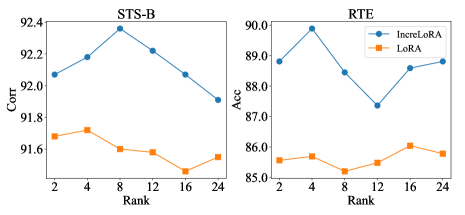
Figure 4: Fine-tuning performance under different parameter budgets. The x-axis represents the average rank, and the y-axis is the evaluation index of different data sets. Set the same learning rate under different parameter budgets.

4.3 Different Budget Levels

We test the performance of IncreLoRA fine-tuning DeBERTaV3-base under different parameter budget levels and present the results in Figure 4. We find that on both the RTE and STS-B datasets, our method achieves significant performance improvements at different budget levels. And IncreLoRA requires only the lowest parameter budget and already exceeds the performance of LoRA for all parameter budget levels. For example, IncreLoRA achieves 88.81% accuracy on RTE when rank equals 2, which is 2.77% higher than the best performance of LoRA (86.04%). This shows that our method has good parameter efficiency in low resource situations.

4.4 Ablation Experiment

In order to verify the effectiveness of the individual components, we perform ablation experiments in the setting of average rank = 2 and display the results in Table 2 and Figure 5. In this section, we focus on the interactions between the components. Note that orthogonal regularization is not our proposed method, but we still include it in the ablation experiments in order to verify its interactions with other components.

Raw Incremental Parameter Allocation

We eliminate all components and simply add trainable parameters dynamically during training, this process is the opposite of structured pruning based on LoRA and produces worse performance. Since the parameters added halfway through the process are not adequately trained, the performance of the model drops dramatically, even lower than the original LoRA.

Advance Learning and Orthogonal Regularization

Adding advance learning and orthogonal regularization individually to the original incremental parameter allocation both significantly improves the training performance of the model. On RTE, orthogonal regularization and advance learning bring 1.81% and 1.08% accuracy improvement, respectively. The focus here on the effect of our proposed advance learning on orthogonal regularization. It can be seen that by adding advance learning to the orthogonal regular term, the accuracy of RTE and the average correlation of STS-B increase by 0.36% and 0.10%, respectively. Zhang et al. (2023) argues that keeping $A$ and $B$ orthogonal improves the parameter efficiency of the model.

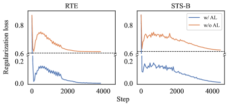
Figure 5: Regularization loss with and without advance learning. To save space, the middle part that does not contain critical information is truncated.

As shown in Figure 5, $A,B$ still has a large orthogonal regularization loss after training, while after adding advance learning, the orthogonal regularization loss decreases rapidly, and $A,B$ has practically orthogonality. We believe this is due to the trade-off between predictive and regularization losses. When advance learning is removed, the added parameter gradient comes more from the prediction loss, which tends to prevent the regularization loss from decreasing. During advance learning, $\lambda_{s}$ is fixed to a smaller value, which limits the influence of the preparatory component on the model, the gradient comes more from the regularization loss, and when the preparatory component is activated, it tends to already have better orthogonality properties, which ensures the parametric efficiency of our method.

Restart Warmup

Although learning in advance allows $w_{i}$ to be activated with a better initial state, when the randomly initialized $a_{i}$ and $b_{i}$ follow the original learning rate scheduler, it is prone to unstable training due to the large variance of the mini-batch data distribution(Goyal et al. 2017). When restarting warmup for each added parameter group, the performance of the model is significantly improved.

4.5 Analysis

In order to verify the validity of the high rank upper bound due to incremental parameter allocations, we investigate the impact of the rank distributions of IncreLoRA and AdaLoRA on the model performance. Specifically, we apply the two methods based on the same base model and parameter scales on the SST-2 respectively and save the rank distributions of their respective individual modules. As shown in Figure 6, both methods favor assigning more rank to $W_{v},W_{o}$ and $W_{f1}$, but IncreLoRA produces a more centralized distribution of rank. We hypothesize that this is one of the factors that make our approach fruitful on low resources, as it ensures that important modules still have a high rank in low resource situations.

Method	#Params	SST-2	#Params	CoLA
		Acc.		Acc.
IncreLoRA	0.35M	96.22	0.32M	71.48
AdaLoRA	0.31M	95.86	0.31M	70.64
LoRA (r = Incre)	0.35M	95.87	0.32M	70.66
LoRA (r = Ada)	0.31M	95.76	0.31M	70.31

Table 3: The rank distributions generated by IncreLoRA and AdaLoRA are used to initialize and retrain the two LoRAs separately. Average rank is 2.

We initialize the two new LoRA models with the two different rank distributions, and in order to minimize the experimental variability, we retain the SVD-like parameter matrix form and regularization terms common to both methods and train them with the same learning rate and number of epochs. As shown in Table 3, the rank distribution obtained by IncreLoRA results in a model with better parameter efficiency. In addition, we find that the performance of the LoRA models with two different rank distributions is not as well as that of IncreLoRA and AdaLoRA, which suggests that the generated rank distributions and our proposed incremental parameter allocation method have some dependence, and only by dynamic adjusting the individual modules during the training process can the optimal performance be achieved.

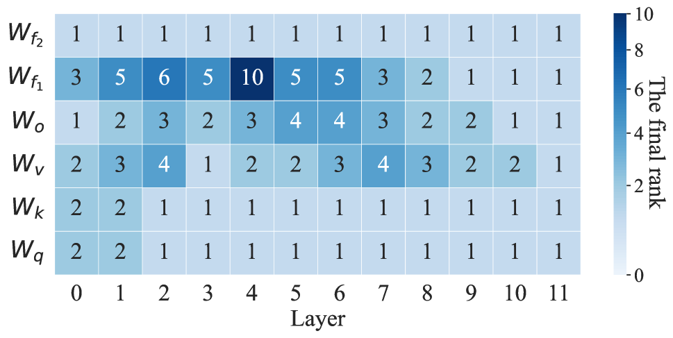
(a) IncreLoRA

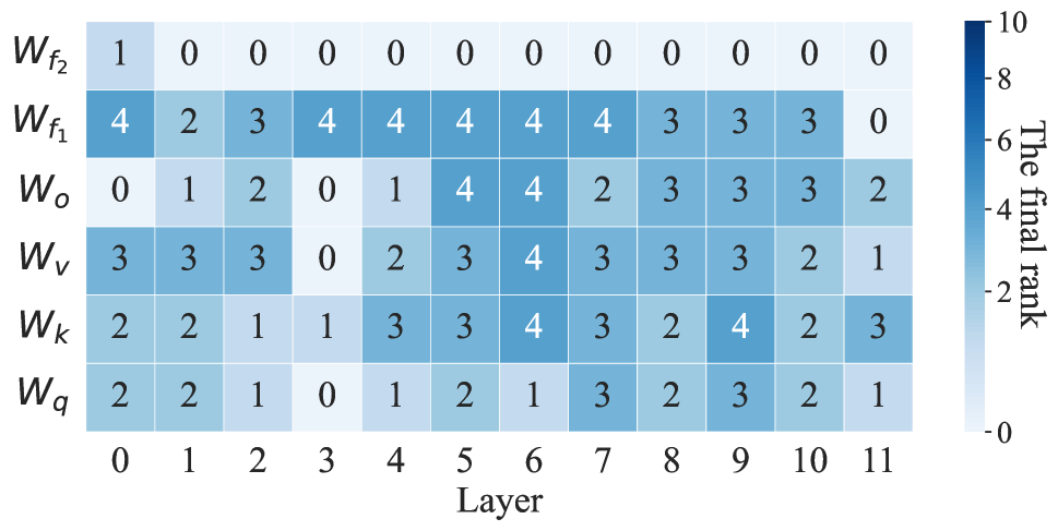
(b) AdaLoRA

Figure 6: The rank of each update matrix after fine-tuning DeBERTaV3-base on SST-2 using IncreLoRA and AdaLoRA, respectively. Where the horizontal coordinate represents the layer index and the vertical coordinate represents the type of module, from bottom to top, query/key/value projection, output projection in the self-attention, and two weight matrices in two-layer FFNs.

5 Conclusion

In this paper, we propose a simple and effective parameter-efficient trimming method, IncreLoRA, for further improving the parameter efficiency of low-rank adapters. Unlike the structured pruning method, we incrementally assign trainable parameters during the training process. In addition, we reconstruct the low-rank matrix in LoRA and propose to utilize early learning and restarting warmup to improve the training effect and stability. Experimental results demonstrate the effectiveness of our proposed model and show superior performance with low resources.

Appendix A GLUE DATASET STATISTICS

We present the summary of the GLUE (Wang et al. 2019) benchmark in the table below, where WNLI is not included in the experiment.

Corpus	Train	Dev	Task	Metrics	Domain
Single-Sentence Task
CoLA	8.5k	1k	acceptability	Matthews corr.	misc.
SST-2	67k	872	sentiment	Acc.	movie reviews
Similarity and Paraphrase Tasks
MRPC	3.7k	408	paraphrase	Acc./F1	news
STS-B	7k	1.5k	sentence similarity	Pearson/Spearman corr.	misc.
QQP	364k	40k	paraphrase	Acc./F1	social QA questions
Inference Tasks
MNLI	393k	20k	NLI	Matched Acc./Mismatched Acc.	misc.
QNLI	105k	5.7k	QA/NLI	Acc.	Wikipedia
RTE	2.5K	276	NLI	Acc.	news,Wikipedia
WNLI	634	71	coreference/NLI	Acc.	fiction books

Table 4: Task descriptions and statistics of GLUE. All tasks are single sentence or sentence pair classification, except STS-B, which is a regression task. MNLI has three classes; all other classification tasks have two.

Appendix B TRAINING DETAILS

In all tasks, batch size, $\beta_{1}$, $\beta_{2}$ in equation (6), (7) are {32, 0.85, 0.85}. we set the allocation interval $\nu$ by default to the same value as warmup steps.

Dataset	learning rate	batch size	epochs	top_h	warmup steps	dropout rate
MNLI	$3.5\times 10^{-4}$	32	9	2	1000	0.2
SST-2	$8\times 10^{-4}$	32	24	5	1000	0.1
CoLA	$8\times 10^{-4}$	32	25	3	100	0
QQP	$4\times 10^{-4}$	32	7	3	1000	0
QNLI	$7\times 10^{-4}$	32	5	12	500	0
RTE	$1.2\times 10^{-3}$	32	50	5	100	0
MRPC	$1\times 10^{-3}$	32	30	6	100	0.3
STS-B	$2.2\times 10^{-3}$	32	25	4	100	0

Appendix C QUESTION ANSWERING TASK

We evaluate the performance of IncreLoRA on a Q&A dataset with the pre-trained model DeBERTaV3-base. SQuADv2.0 is available at https://rajpurkar.github.io/SQuAD-explorer/.

	SQuADv2.0
Full FT	85.4/88.4
# Params	0.16%	0.32%	0.65%
HAdapter	84.3/87.3	84.9/87.9	85.4/88.3
PAdapter	84.5/87.6	84.9/87.8	84.5/87.5
LoRA	83.6/86.7	84.5/87.4	85.0/88.0
AdaLoRA	85.7/88.8	85.5/88.6	86.0/88.9
IncreLoRA	86.05/88.81	85.89/88.84	86.17/89.07

Table 5: Results with DeBERTaV3-base on SQuADv2.0. Here Params is the number of trainable parameters relative to that in full fine-tuning. We report EM/F1. The best results in each setting are shown in bold.

Appendix D EXPERIMENTAL STATISTICS

We fine-tune DeBERTaV3-base on eight datasets using IncreLoRA and present the statistical results of the scaling ($\lambda$) for all module components ($w$) in the figure below, where all weights are taken as absolute values. It can be observed that most singular values fall within the range of 1e-1 to 1e-2.

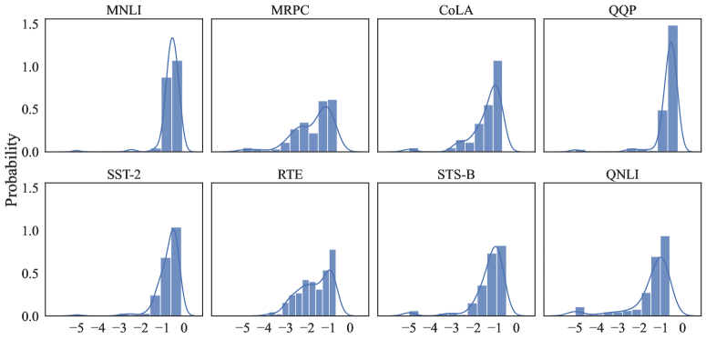
Figure 7: Scaling factor statistic plots. The horizontal axis represents the power of the scaling factor, the vertical axis represents the probability density.

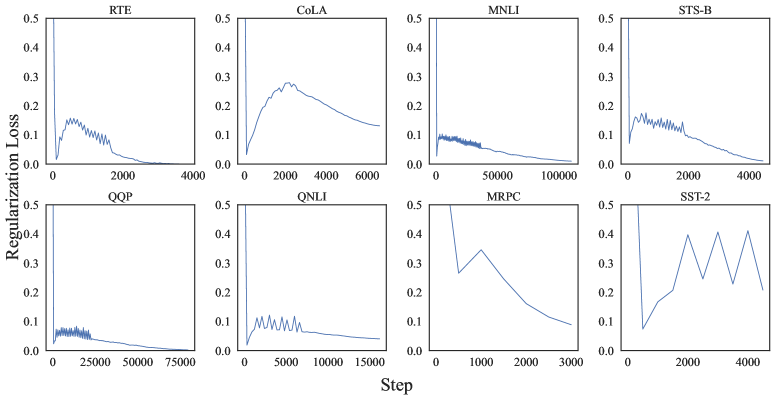
Figure 8: Orthogonal Regularization loss on all eight tasks.

References

- Ansell et al. (2022) Ansell, A.; Ponti, E. M.; Korhonen, A.; and Vulic, I. 2022. Composable Sparse Fine-Tuning for Cross-Lingual Transfer. In Muresan, S.; Nakov, P.; and Villavicencio, A., eds., Proceedings of the 60th Annual Meeting of the Association for Computational Linguistics (Volume 1: Long Papers), ACL 2022, Dublin, Ireland, May 22-27, 2022, 1778–1796. Association for Computational Linguistics.
- Bai et al. (2022) Bai, Y.; Wang, H.; Ma, X.; Zhang, Y.; Tao, Z.; and Fu, Y. 2022. Parameter-Efficient Masking Networks. In NeurIPS.
- Brown et al. (2020) Brown, T. B.; Mann, B.; Ryder, N.; Subbiah, M.; Kaplan, J.; Dhariwal, P.; Neelakantan, A.; Shyam, P.; Sastry, G.; Askell, A.; Agarwal, S.; Herbert-Voss, A.; Krueger, G.; Henighan, T.; Child, R.; Ramesh, A.; Ziegler, D. M.; Wu, J.; Winter, C.; Hesse, C.; Chen, M.; Sigler, E.; Litwin, M.; Gray, S.; Chess, B.; Clark, J.; Berner, C.; McCandlish, S.; Radford, A.; Sutskever, I.; and Amodei, D. 2020. Language Models are Few-Shot Learners. In Larochelle, H.; Ranzato, M.; Hadsell, R.; Balcan, M.; and Lin, H., eds., Advances in Neural Information Processing Systems 33: Annual Conference on Neural Information Processing Systems 2020, NeurIPS 2020, December 6-12, 2020, virtual.
- Chen et al. (2023) Chen, J.; Zhang, A.; Shi, X.; Li, M.; Smola, A.; and Yang, D. 2023. Parameter-Efficient Fine-Tuning Design Spaces. In The Eleventh International Conference on Learning Representations, ICLR 2023, Kigali, Rwanda, May 1-5, 2023. OpenReview.net.
- Dettmers et al. (2023) Dettmers, T.; Pagnoni, A.; Holtzman, A.; and Zettlemoyer, L. 2023. QLoRA: Efficient Finetuning of Quantized LLMs. CoRR, abs/2305.14314.
- Devlin et al. (2019) Devlin, J.; Chang, M.; Lee, K.; and Toutanova, K. 2019. BERT: Pre-training of Deep Bidirectional Transformers for Language Understanding. In Burstein, J.; Doran, C.; and Solorio, T., eds., Proceedings of the 2019 Conference of the North American Chapter of the Association for Computational Linguistics: Human Language Technologies, NAACL-HLT 2019, Minneapolis, MN, USA, June 2-7, 2019, Volume 1 (Long and Short Papers), 4171–4186. Association for Computational Linguistics.
- Donahue et al. (2014) Donahue, J.; Jia, Y.; Vinyals, O.; Hoffman, J.; Zhang, N.; Tzeng, E.; and Darrell, T. 2014. DeCAF: A Deep Convolutional Activation Feature for Generic Visual Recognition. In Proceedings of the 31th International Conference on Machine Learning, ICML 2014, Beijing, China, 21-26 June 2014, volume 32 of JMLR Workshop and Conference Proceedings, 647–655. JMLR.org.
- Gheini, Ren, and May (2021) Gheini, M.; Ren, X.; and May, J. 2021. Cross-Attention is All You Need: Adapting Pretrained Transformers for Machine Translation. In Moens, M.; Huang, X.; Specia, L.; and Yih, S. W., eds., Proceedings of the 2021 Conference on Empirical Methods in Natural Language Processing, EMNLP 2021, Virtual Event / Punta Cana, Dominican Republic, 7-11 November, 2021, 1754–1765. Association for Computational Linguistics.
- Goyal et al. (2017) Goyal, P.; Dollár, P.; Girshick, R. B.; Noordhuis, P.; Wesolowski, L.; Kyrola, A.; Tulloch, A.; Jia, Y.; and He, K. 2017. Accurate, Large Minibatch SGD: Training ImageNet in 1 Hour. CoRR, abs/1706.02677.
- Guo, Rush, and Kim (2021a) Guo, D.; Rush, A. M.; and Kim, Y. 2021a. Parameter-Efficient Transfer Learning with Diff Pruning. In Zong, C.; Xia, F.; Li, W.; and Navigli, R., eds., Proceedings of the 59th Annual Meeting of the Association for Computational Linguistics and the 11th International Joint Conference on Natural Language Processing, ACL/IJCNLP 2021, (Volume 1: Long Papers), Virtual Event, August 1-6, 2021, 4884–4896. Association for Computational Linguistics.
- Guo, Rush, and Kim (2021b) Guo, D.; Rush, A. M.; and Kim, Y. 2021b. Parameter-Efficient Transfer Learning with Diff Pruning. In Zong, C.; Xia, F.; Li, W.; and Navigli, R., eds., Proceedings of the 59th Annual Meeting of the Association for Computational Linguistics and the 11th International Joint Conference on Natural Language Processing, ACL/IJCNLP 2021, (Volume 1: Long Papers), Virtual Event, August 1-6, 2021, 4884–4896. Association for Computational Linguistics.
- He et al. (2022a) He, J.; Zhou, C.; Ma, X.; Berg-Kirkpatrick, T.; and Neubig, G. 2022a. Towards a Unified View of Parameter-Efficient Transfer Learning. In The Tenth International Conference on Learning Representations, ICLR 2022, Virtual Event, April 25-29, 2022. OpenReview.net.
- He, Gao, and Chen (2023) He, P.; Gao, J.; and Chen, W. 2023. DeBERTaV3: Improving DeBERTa using ELECTRA-Style Pre-Training with Gradient-Disentangled Embedding Sharing. In The Eleventh International Conference on Learning Representations, ICLR 2023, Kigali, Rwanda, May 1-5, 2023. OpenReview.net.
- He et al. (2022b) He, S.; Ding, L.; Dong, D.; Zhang, J.; and Tao, D. 2022b. SparseAdapter: An Easy Approach for Improving the Parameter-Efficiency of Adapters. In Goldberg, Y.; Kozareva, Z.; and Zhang, Y., eds., Findings of the Association for Computational Linguistics: EMNLP 2022, Abu Dhabi, United Arab Emirates, December 7-11, 2022, 2184–2190. Association for Computational Linguistics.
- Houlsby et al. (2019a) Houlsby, N.; Giurgiu, A.; Jastrzebski, S.; Morrone, B.; de Laroussilhe, Q.; Gesmundo, A.; Attariyan, M.; and Gelly, S. 2019a. Parameter-Efficient Transfer Learning for NLP. In Chaudhuri, K.; and Salakhutdinov, R., eds., Proceedings of the 36th International Conference on Machine Learning, ICML 2019, 9-15 June 2019, Long Beach, California, USA, volume 97 of Proceedings of Machine Learning Research, 2790–2799. PMLR.
- Houlsby et al. (2019b) Houlsby, N.; Giurgiu, A.; Jastrzebski, S.; Morrone, B.; de Laroussilhe, Q.; Gesmundo, A.; Attariyan, M.; and Gelly, S. 2019b. Parameter-Efficient Transfer Learning for NLP. In Chaudhuri, K.; and Salakhutdinov, R., eds., Proceedings of the 36th International Conference on Machine Learning, ICML 2019, 9-15 June 2019, Long Beach, California, USA, volume 97 of Proceedings of Machine Learning Research, 2790–2799. PMLR.
- Hu et al. (2022) Hu, E. J.; Shen, Y.; Wallis, P.; Allen-Zhu, Z.; Li, Y.; Wang, S.; Wang, L.; and Chen, W. 2022. LoRA: Low-Rank Adaptation of Large Language Models. In The Tenth International Conference on Learning Representations, ICLR 2022, Virtual Event, April 25-29, 2022. OpenReview.net.
- Lawton et al. (2023) Lawton, N.; Kumar, A.; Thattai, G.; Galstyan, A.; and Steeg, G. V. 2023. Neural Architecture Search for Parameter-Efficient Fine-tuning of Large Pre-trained Language Models. In Rogers, A.; Boyd-Graber, J. L.; and Okazaki, N., eds., Findings of the Association for Computational Linguistics: ACL 2023, Toronto, Canada, July 9-14, 2023, 8506–8515. Association for Computational Linguistics.
- Lester, Al-Rfou, and Constant (2021a) Lester, B.; Al-Rfou, R.; and Constant, N. 2021a. The Power of Scale for Parameter-Efficient Prompt Tuning. In Moens, M.; Huang, X.; Specia, L.; and Yih, S. W., eds., Proceedings of the 2021 Conference on Empirical Methods in Natural Language Processing, EMNLP 2021, Virtual Event / Punta Cana, Dominican Republic, 7-11 November, 2021, 3045–3059. Association for Computational Linguistics.
- Lester, Al-Rfou, and Constant (2021b) Lester, B.; Al-Rfou, R.; and Constant, N. 2021b. The Power of Scale for Parameter-Efficient Prompt Tuning. In Moens, M.; Huang, X.; Specia, L.; and Yih, S. W., eds., Proceedings of the 2021 Conference on Empirical Methods in Natural Language Processing, EMNLP 2021, Virtual Event / Punta Cana, Dominican Republic, 7-11 November, 2021, 3045–3059. Association for Computational Linguistics.
- Li and Liang (2021) Li, X. L.; and Liang, P. 2021. Prefix-Tuning: Optimizing Continuous Prompts for Generation. In Zong, C.; Xia, F.; Li, W.; and Navigli, R., eds., Proceedings of the 59th Annual Meeting of the Association for Computational Linguistics and the 11th International Joint Conference on Natural Language Processing, ACL/IJCNLP 2021, (Volume 1: Long Papers), Virtual Event, August 1-6, 2021, 4582–4597. Association for Computational Linguistics.
- Liu et al. (2019) Liu, Y.; Ott, M.; Goyal, N.; Du, J.; Joshi, M.; Chen, D.; Levy, O.; Lewis, M.; Zettlemoyer, L.; and Stoyanov, V. 2019. RoBERTa: A Robustly Optimized BERT Pretraining Approach. CoRR, abs/1907.11692.
- Mahabadi, Henderson, and Ruder (2021) Mahabadi, R. K.; Henderson, J.; and Ruder, S. 2021. Compacter: Efficient Low-Rank Hypercomplex Adapter Layers. In Ranzato, M.; Beygelzimer, A.; Dauphin, Y. N.; Liang, P.; and Vaughan, J. W., eds., Advances in Neural Information Processing Systems 34: Annual Conference on Neural Information Processing Systems 2021, NeurIPS 2021, December 6-14, 2021, virtual, 1022–1035.
- Mao et al. (2022) Mao, Y.; Mathias, L.; Hou, R.; Almahairi, A.; Ma, H.; Han, J.; Yih, S.; and Khabsa, M. 2022. UniPELT: A Unified Framework for Parameter-Efficient Language Model Tuning. In Muresan, S.; Nakov, P.; and Villavicencio, A., eds., Proceedings of the 60th Annual Meeting of the Association for Computational Linguistics (Volume 1: Long Papers), ACL 2022, Dublin, Ireland, May 22-27, 2022, 6253–6264. Association for Computational Linguistics.
- Molchanov et al. (2019) Molchanov, P.; Mallya, A.; Tyree, S.; Frosio, I.; and Kautz, J. 2019. Importance Estimation for Neural Network Pruning. In IEEE Conference on Computer Vision and Pattern Recognition, CVPR 2019, Long Beach, CA, USA, June 16-20, 2019, 11264–11272. Computer Vision Foundation / IEEE.
- Paszke et al. (2019) Paszke, A.; Gross, S.; Massa, F.; Lerer, A.; Bradbury, J.; Chanan, G.; Killeen, T.; Lin, Z.; Gimelshein, N.; Antiga, L.; Desmaison, A.; Köpf, A.; Yang, E. Z.; DeVito, Z.; Raison, M.; Tejani, A.; Chilamkurthy, S.; Steiner, B.; Fang, L.; Bai, J.; and Chintala, S. 2019. PyTorch: An Imperative Style, High-Performance Deep Learning Library. In Wallach, H. M.; Larochelle, H.; Beygelzimer, A.; d’Alché-Buc, F.; Fox, E. B.; and Garnett, R., eds., Advances in Neural Information Processing Systems 32: Annual Conference on Neural Information Processing Systems 2019, NeurIPS 2019, December 8-14, 2019, Vancouver, BC, Canada, 8024–8035.
- Peters et al. (2018) Peters, M. E.; Neumann, M.; Iyyer, M.; Gardner, M.; Clark, C.; Lee, K.; and Zettlemoyer, L. 2018. Deep Contextualized Word Representations. In Walker, M. A.; Ji, H.; and Stent, A., eds., Proceedings of the 2018 Conference of the North American Chapter of the Association for Computational Linguistics: Human Language Technologies, NAACL-HLT 2018, New Orleans, Louisiana, USA, June 1-6, 2018, Volume 1 (Long Papers), 2227–2237. Association for Computational Linguistics.
- Pfeiffer et al. (2021) Pfeiffer, J.; Kamath, A.; Rücklé, A.; Cho, K.; and Gurevych, I. 2021. AdapterFusion: Non-Destructive Task Composition for Transfer Learning. In Merlo, P.; Tiedemann, J.; and Tsarfaty, R., eds., Proceedings of the 16th Conference of the European Chapter of the Association for Computational Linguistics: Main Volume, EACL 2021, Online, April 19 - 23, 2021, 487–503. Association for Computational Linguistics.
- Radford et al. (2021) Radford, A.; Kim, J. W.; Hallacy, C.; Ramesh, A.; Goh, G.; Agarwal, S.; Sastry, G.; Askell, A.; Mishkin, P.; Clark, J.; Krueger, G.; and Sutskever, I. 2021. Learning Transferable Visual Models From Natural Language Supervision. In Meila, M.; and Zhang, T., eds., Proceedings of the 38th International Conference on Machine Learning, ICML 2021, 18-24 July 2021, Virtual Event, volume 139 of Proceedings of Machine Learning Research, 8748–8763. PMLR.
- Radford et al. (2018) Radford, A.; Narasimhan, K.; Salimans, T.; Sutskever, I.; et al. 2018. Improving language understanding by generative pre-training.
- Raffel et al. (2020) Raffel, C.; Shazeer, N.; Roberts, A.; Lee, K.; Narang, S.; Matena, M.; Zhou, Y.; Li, W.; and Liu, P. J. 2020. Exploring the Limits of Transfer Learning with a Unified Text-to-Text Transformer. J. Mach. Learn. Res., 21: 140:1–140:67.
- Rebuffi, Bilen, and Vedaldi (2017) Rebuffi, S.; Bilen, H.; and Vedaldi, A. 2017. Learning multiple visual domains with residual adapters. In Guyon, I.; von Luxburg, U.; Bengio, S.; Wallach, H. M.; Fergus, R.; Vishwanathan, S. V. N.; and Garnett, R., eds., Advances in Neural Information Processing Systems 30: Annual Conference on Neural Information Processing Systems 2017, December 4-9, 2017, Long Beach, CA, USA, 506–516.
- Smith et al. (2023) Smith, J. S.; Hsu, Y.; Zhang, L.; Hua, T.; Kira, Z.; Shen, Y.; and Jin, H. 2023. Continual Diffusion: Continual Customization of Text-to-Image Diffusion with C-LoRA. CoRR, abs/2304.06027.
- Sung, Cho, and Bansal (2022) Sung, Y.; Cho, J.; and Bansal, M. 2022. LST: Ladder Side-Tuning for Parameter and Memory Efficient Transfer Learning. In NeurIPS.
- Sung, Nair, and Raffel (2021a) Sung, Y.; Nair, V.; and Raffel, C. 2021a. Training Neural Networks with Fixed Sparse Masks. In Ranzato, M.; Beygelzimer, A.; Dauphin, Y. N.; Liang, P.; and Vaughan, J. W., eds., Advances in Neural Information Processing Systems 34: Annual Conference on Neural Information Processing Systems 2021, NeurIPS 2021, December 6-14, 2021, virtual, 24193–24205.
- Sung, Nair, and Raffel (2021b) Sung, Y.; Nair, V.; and Raffel, C. 2021b. Training Neural Networks with Fixed Sparse Masks. In Ranzato, M.; Beygelzimer, A.; Dauphin, Y. N.; Liang, P.; and Vaughan, J. W., eds., Advances in Neural Information Processing Systems 34: Annual Conference on Neural Information Processing Systems 2021, NeurIPS 2021, December 6-14, 2021, virtual, 24193–24205.
- Touvron et al. (2023) Touvron, H.; Lavril, T.; Izacard, G.; Martinet, X.; Lachaux, M.; Lacroix, T.; Rozière, B.; Goyal, N.; Hambro, E.; Azhar, F.; Rodriguez, A.; Joulin, A.; Grave, E.; and Lample, G. 2023. LLaMA: Open and Efficient Foundation Language Models. CoRR, abs/2302.13971.
- Vaswani et al. (2017) Vaswani, A.; Shazeer, N.; Parmar, N.; Uszkoreit, J.; Jones, L.; Gomez, A. N.; Kaiser, L.; and Polosukhin, I. 2017. Attention is All you Need. In Guyon, I.; von Luxburg, U.; Bengio, S.; Wallach, H. M.; Fergus, R.; Vishwanathan, S. V. N.; and Garnett, R., eds., Advances in Neural Information Processing Systems 30: Annual Conference on Neural Information Processing Systems 2017, December 4-9, 2017, Long Beach, CA, USA, 5998–6008.
- Vucetic et al. (2022) Vucetic, D.; Tayaranian, M.; Ziaeefard, M.; Clark, J. J.; Meyer, B. H.; and Gross, W. J. 2022. Efficient Fine-Tuning of BERT Models on the Edge. In IEEE International Symposium on Circuits and Systems, ISCAS 2022, Austin, TX, USA, May 27 - June 1, 2022, 1838–1842. IEEE.
- Wang et al. (2019) Wang, A.; Singh, A.; Michael, J.; Hill, F.; Levy, O.; and Bowman, S. R. 2019. GLUE: A Multi-Task Benchmark and Analysis Platform for Natural Language Understanding. In 7th International Conference on Learning Representations, ICLR 2019, New Orleans, LA, USA, May 6-9, 2019. OpenReview.net.
- Wang et al. (2022) Wang, Y.; Mukherjee, S.; Liu, X.; Gao, J.; Awadallah, A. H.; and Gao, J. 2022. AdaMix: Mixture-of-Adapter for Parameter-efficient Tuning of Large Language Models. CoRR, abs/2205.12410.
- Zaken, Goldberg, and Ravfogel (2022) Zaken, E. B.; Goldberg, Y.; and Ravfogel, S. 2022. BitFit: Simple Parameter-efficient Fine-tuning for Transformer-based Masked Language-models. In Muresan, S.; Nakov, P.; and Villavicencio, A., eds., Proceedings of the 60th Annual Meeting of the Association for Computational Linguistics (Volume 2: Short Papers), ACL 2022, Dublin, Ireland, May 22-27, 2022, 1–9. Association for Computational Linguistics.
- Zeng, Zhang, and Lu (2023) Zeng, G.; Zhang, P.; and Lu, W. 2023. One Network, Many Masks: Towards More Parameter-Efficient Transfer Learning. In Rogers, A.; Boyd-Graber, J. L.; and Okazaki, N., eds., Proceedings of the 61st Annual Meeting of the Association for Computational Linguistics (Volume 1: Long Papers), ACL 2023, Toronto, Canada, July 9-14, 2023, 7564–7580. Association for Computational Linguistics.
- Zhang et al. (2023) Zhang, Q.; Chen, M.; Bukharin, A.; He, P.; Cheng, Y.; Chen, W.; and Zhao, T. 2023. Adaptive Budget Allocation for Parameter-Efficient Fine-Tuning. In The Eleventh International Conference on Learning Representations, ICLR 2023, Kigali, Rwanda, May 1-5, 2023. OpenReview.net.
- Zhang et al. (2022) Zhang, Q.; Zuo, S.; Liang, C.; Bukharin, A.; He, P.; Chen, W.; and Zhao, T. 2022. PLATON: Pruning Large Transformer Models with Upper Confidence Bound of Weight Importance. In Chaudhuri, K.; Jegelka, S.; Song, L.; Szepesvári, C.; Niu, G.; and Sabato, S., eds., International Conference on Machine Learning, ICML 2022, 17-23 July 2022, Baltimore, Maryland, USA, volume 162 of Proceedings of Machine Learning Research, 26809–26823. PMLR.