Digital-analog quantum computing of fermion-boson models in superconducting circuits

Abstract

We propose a digital-analog quantum algorithm for simulating the Hubbard-Holstein model, describing strongly-correlated fermion-boson interactions, in a suitable architecture with superconducting circuits. It comprises a linear chain of qubits connected by resonators, emulating electron-electron (e-e) and electron-phonon (e-p) interactions, as well as fermion tunneling. Our approach is adequate for a digital-analog quantum computing (DAQC) of fermion-boson models including those described by the Hubbard-Holstein model. We show the reduction in the circuit depth of the DAQC algorithm, a sequence of digital steps and analog blocks, outperforming the purely digital approach. We exemplify the quantum simulation of a half-filling two-site Hubbard-Holstein model. In such example we obtain fidelities larger than 0.98, showing that our proposal is suitable to study the dynamical behavior of solid-state systems. Our proposal opens the door to computing complex systems for chemistry, materials, and high-energy physics.

Introduction. In solid-state physics, the Hubbard-Holstein (HH) model is commonly used to describe fermionic lattices interacting with phonons [1]. This model captures a range of phenomena, such as polaron and bipolaron formation [2, 3, 4]. It plays a vital role in determining the transport properties of biomolecules [5, 6], as well as correlation effects and localization phenomena in materials like cuprates, fullerides, and manganites [7, 8, 9, 10]. Consequently, the HH model and similar systems, describing fermionic lattices coupled to bosons, are fundamental in various research fields and technologies in chemistry, materials, and high-energy physics.

Strongly correlated fermionic systems, including those involving fermion-phonon interactions, pose significant challenges due to the complex nature of many-body systems. Achieving exact solutions for general fermionic systems becomes impractical beyond a few particles, leading to the need for approximations and symmetry conditions. Various theoretical and computational techniques have been developed to address these challenges, including mean-field theories [11, 12, 13], quantum Monte Carlo methods [14, 15], density functional theory [16], tensor network methods [17], and the density matrix renormalization group algorithm [18]. These approaches provide ways to approximate the behavior of many-body systems and gain insights into their properties, although mean-field theories overlook crucial correlation effects. These techniques play a crucial role in advancing technology in the era of the second quantum revolution.

Quantum simulation and quantum computing offer advanced approaches to studying the dynamics of strongly-correlated systems [19]. By encoding the targeted model into controllable quantum processors, the quantum evolution can be mimicked in a digital, analog, or digital-analog manner. In digital simulations, a specific sequence of single-qubit and two-qubit gates, forming a universal set of quantum logic gates, is used to emulate any quantum evolution. However, the fidelity of single and two-qubit gates, as well as qubit coherences, limit the usefulness of this approach in our noisy intermediate-scale quantum (NISQ) era. In contrast, analog simulations naturally perform the desired quantum evolution within specific parameter ranges with a high accuracy, but it only works for the proposed specific model. An example is the quantum simulation of light-matter interactions in trapped ions [20, 21] and superconducting circuits [22]. A merged approach called digital-analog quantum computing (DAQC) [23] bridges the gap between these two paradigms. DAQC leverages analog dynamics from the simulator Hamiltonian, in the spirit of analog blocks, which are combined with digital steps, using the Trotter-Suzuki expansion in algorithmic manner.

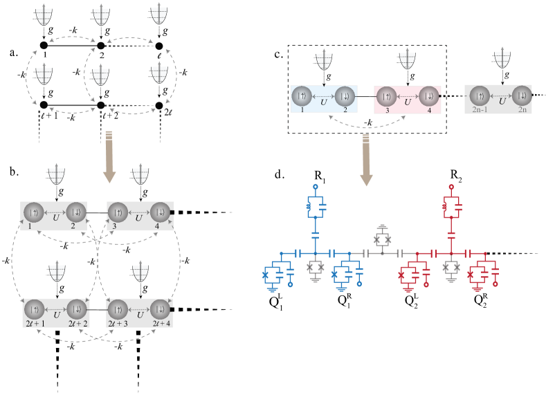
Figure 1: a. The HH lattice to be simulated. b. Mapping of HH lattice to an equivalent spinless fermion lattice. c. Mapping of spinless fermion lattice to a spin chain coupled to bosons using JW transformation. d. Superconducting circuit architecture representing the spin-boson chain.

Quantum simulations have been proposed for studying strongly-correlated fermionic systems, including e-p interactions, on various platforms such as trapped ions [24], cold atoms [25, 26], and superconducting circuits [27, 28]. The key challenge lies in mapping fermionic degrees of freedom onto spin degrees of freedom, achieved for example through the Jordan-Wigner transformation. Trapped ions benefit from the Mølmer-Sørensen gate, be as a well-behaved two-qubit gate or a multiqubit quantum operation. Alternatively, superconducting architectures have also been advanced, demonstrating comparable scalability features through parallel interactions and geometric considerations [29]. Moreover, superconducting circuits offer an ideal platform for compact digital-analog quantum simulations of strongly-correlated fermionic systems with multiple bosonic modes, like the Hubbard-Holstein model. Such versatility is due to the possible addition of multiple waveguide cavities or LC oscillators.

We present a superconducting circuit design for compact simulation of the HH model within the DAQC paradigm, applicable to one- and two-dimensional arrays. Our design comprises qubits, resonators, and superconducting quantum interference devices (SQUIDs) arranged along a chain. This architecture enables natural qubit-resonator and tunable qubit-qubit interactions, facilitating the implementation of analog blocks to encode the evolution under the HH model. We employ the DAQC protocol on a toy model of a half-filling two-site HH Hamiltonian, numerically calculating the fidelity respect to the exact evolution. Comparing our results to a purely digital approach, we obtain an enhanced accuracy. Furthermore, by evaluating resource scaling in terms of gate count, we surpass the performance of existing trapped-ion platforms. Our proposal is thus relevant for exploring phase diagrams, polaron formation, and applications in materials, with implications in chemistry and high-energy physics.

Hubbard-Holstein model.- The HH model describes how electrons on a lattice interact due to their fermionic character and also with phononic vibrations. These include e-p interactions, e-e repulsion, and electron hopping between lattice sites. For an $N$-site lattice, the model is described by the Hamiltonian

$$H = \omega_{0}\sum_{j=1}^{N}a_{j}^{\dagger}a_{j}+U\sum_{j=1}^{N}(\hat{n}_{j\uparrow}\hat{n}_{j\downarrow})$$ (1)

$$-k\sum_{\langle j,k\rangle}\sum_{\sigma=\uparrow,\downarrow}(c_{j,\sigma}^{\dagger}c_{k,\sigma}+c_{k,\sigma}^{\dagger}c_{j\sigma})+$$

$$+g\sum_{j=1}^{N}\sum_{\sigma=\uparrow,\downarrow}[\hat{n}_{j,\sigma}(a_{j}^{\dagger}+a_{j})],$$

where $c_{j\sigma}^{\dagger}(c_{j\sigma})$ is the creation (annihilation) fermionic operator for the site $j$ and spin $\sigma$, $a_{i}^{\dagger}(a_{i})$ is the creation (annihilation) operator for the $j$th bosonic mode, and $\hat{n}_{i\sigma}=c_{i\sigma}^{\dagger}c_{i\sigma}$. The parameters $\omega_{0}$ and $U$ are bosonic frequency and on-site Coulomb interaction, respectively. From the coupling terms, $k$ gives the hopping energy in the lattice, where $\langle i,j\rangle$ refers to nearest-neighbour sites, and $g$ represents the e-p coupling strength. We note that if $\omega_{0}=g=0$ (without bosonic modes), the resulting Hamiltonian correspond to the Hubbard model. On the other hand, if $U=0$ (fermions without charge), we obtain the Holstein model.

To simulate the HH model, we need to encode the bosonic and fermionic degrees of freedom. For the first one, in superconducting circuits we can use transmission lines or $LC$ oscillators, obtaining an analog to the phonons in the HH model. On the other hand, the fermion operators (with spin) can be mapped to spinless fermion operators in a lattice of double size, that is $c_{j,\uparrow}\rightarrow b_{2j}$ and $c_{j,\downarrow}\rightarrow b_{2j+1}$. Finally, to encode spinless fermionic operators, we perform the Jordan-Wigner (JW) transformation [30, 31], $b_{j}\rightarrow\prod_{j=1}^{i-1}(-\sigma_{j}^{z})\sigma_{i}^{-}$. In this manner, we map the HH lattice to a spin chain interacting with bosonic modes (see Fig. 1). The latter can be described by the Hamiltonian

$$H= \sum_{j=1}^{N}\Big{[}\omega_{0}a_{j}^{\dagger}a_{j}+\frac{\bar{U}}{4}(\sigma_{2j}^{z}+\sigma_{2j-1}^{z})+\frac{U}{4}(\sigma_{2j}^{z}\sigma_{2j-1}^{z})$$

$$+\frac{g}{2}(\sigma_{2j}^{z}+\sigma_{2j-1}^{z})(a_{j}^{\dagger}+a_{j})\Big{]}$$

$$-k\sum_{\langle j,k\rangle}\Bigg{[}\sigma_{2k}^{-}\bigg{(}\prod_{l=2k}^{2j-1}-\sigma_{l}^{z}\bigg{)}\sigma_{2j}^{+}$$

$$+\sigma_{2k-1}^{-}\bigg{(}\prod_{l=2k-1}^{2j-2}-\sigma_{l}^{z}\bigg{)}\sigma_{2j-1}^{+}+{\rm H.c.}\Bigg{]},$$ (2)

where the term $g(a_{j}+a_{j}^{\dagger})$ was absorbed by the change $a_{j}\rightarrow a_{j}+g/\omega_{0}$, therefore $\bar{U}=U-4g^{2}/\omega_{0}$. We can see that the first and second term in Eq. (2) correspond to the free energy of bosonic and spin degrees of freedom, easily implementable by a set of $LC$ oscillators (or transmission lines) and qubits. The next two terms represent the qubit-qubit and qubit-boson interactions, which can be done in superconducting circuits using capacitive coupling and local rotations in the qubits. The last terms correspond to the fermionic tuneling terms, which can be implemented by using consecutive two-body rotations as shown in Ref. [29].

DAQC with superconducting circuits.- We describe here an architecture that allows to implement efficiently the Hamiltonian of Eq. (2), consisting of a chain of qubits coupled to a set of resonators. To simulate that Hamiltonian, we propose the superconducting circuit architecture displayed in Fig. 1b. Such superconducting design consists in a linear array of transmon qubits coupled through grounded superconducting quantum interference devices (SQUIDs). In addition, the chain of qubits has LC resonators coupled at each site by grounded SQUIDs. For the transmon array, we interspersed devices with different spectra. It means that nearest neighbour qubits are off-resonance, then the qubits in odd positions have different frequency that the qubits in even positions, as well as the resonators have a different frequency with respect to the qubits. Therefore, our architecture can be seen as a chain of building blocks, enclosed by a dashed square in Fig 1, composed of three different devices, a left qubit with frequency $\omega_{L}$, a right qubit with frequency $\omega_{R}$, and a resonator with frequency $\omega$. A similar architecure without resonators was proposed in Ref. [29], and another including resonators experimentally done in Ref. [32], both in the context of quantum simulations.

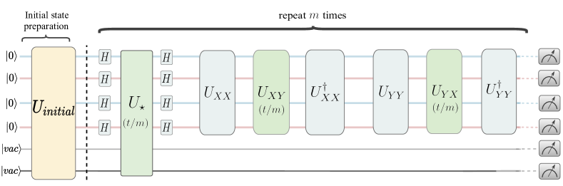
Figure 2: DAQC circuit for a 2-site HH model. The gates in green are the analog blocks while the blue ones are the digital steps. The circuit depth is $9$ which does not scale as we add more sites in the 1D array.

After high-plasma frequency and low impedance SQUID approximations, our architecture is described by the next interaction-picture Hamiltonian

$$H=\sum_{j=1}^{N}H_{s}^{(j)}+\sum_{j=1}^{n-1}H_{s-s}^{(j)}\,,$$ (3)

where $H_{s}^{(j)}$ and $H_{s-s}^{(j)}$ are the $j$th building-block Hamiltonian and the interaction between building-blocks $j$ and $j+1$, respectively. Such Hamiltonians have the form (for a detailed calculation see the Appendix)

$$H_{s}^{(j)}= \frac{m_{1}A_{QQ}}{4}\Big{[}C_{QQ}^{+}\sigma_{L,j}^{x}\sigma_{R,j}^{x}-S_{QQ}^{+}\sigma_{L,j}^{x}\sigma_{R,j}^{y}+S_{QQ}^{-}\sigma_{L,j}^{y}\sigma_{R,j}^{x}+C_{QQ}^{-}\sigma_{L,j}^{y}\sigma_{R,j}^{y}\Big{]}$$

$$+\frac{1}{4}\sum_{\alpha=\{L,R\}}A_{QR}l_{1}^{\alpha}\Big{[}C_{QR}^{+}\sigma_{\alpha,j}^{x}(a_{j}^{\dagger}-a_{j})-C_{QR}^{-}\sigma_{\alpha,j}^{y}(a_{j}^{\dagger}+a_{j})+S_{QR}^{+}\sigma_{\alpha,j}^{x}(a_{j}^{\dagger}+a_{j})-S_{QR}^{-}\sigma_{\alpha,j}^{y}(a_{j}^{\dagger}-a_{j})\Big{]},$$

$$H_{s-s}^{(j)} =\frac{m_{1}\bar{A}_{QQ}}{4}\Big{[}C_{\phi QQ}^{+}\sigma_{R,j}^{x}\sigma_{L,j+1}^{x}-S_{\phi QQ}^{+}\sigma_{R,j}^{x}\sigma_{L,j+1}^{y}+S_{\phi QQ}^{-}\sigma_{R,j}^{y}\sigma_{L,j+1}^{x}+C_{\phi QQ}^{-}\sigma_{R,j}^{y}\sigma_{L,j+1}^{y}\Big{]},$$ (4)

where $C_{ab}^{\pm}=\cos\tilde{\varphi}_{ab}^{+}\pm\cos\tilde{\varphi}_{ab}^{-}$, $\tilde{C}_{ab}^{\pm}=\cos\tilde{\phi}_{ab}^{+}\pm\cos\tilde{\phi}_{ab}^{-}$, and similar definitions for $S_{ab}^{\pm}$ and $S_{ab}^{\pm}$, replacing $\sin$ by $\cos$. $\tilde{\varphi}_{ab}^{\pm}$ are the phases asociated to the magnetic flux through the SQUIDs inside of each building-block, and $\tilde{\phi}_{ab}^{\pm}$ are the pases of the magnetic flux through the SQUIDs that couple different building blocks. We note that adjusting the different phases we can engineer a wide range qubit-qubit and qubit-boson interactions.

We will now focus in mimicking each interaction term of the target Hamiltonian of Eq. (2). The Coulomb repulsion $\sigma_{2j}^{z}\sigma_{2j-1}^{z}=\sigma_{L,j}^{z}\sigma_{R,j}^{z}$ and the e-p terms can be realized simultaneously by turning off all the magnetic fluxes ($A_{QQ}=A_{QR}^{(j)}=\bar{A}_{QQ}=0$), applying a Hadamard gate over each qubit, then turn on the signal $QQ$ and $QR$ in each building block ($A_{QQ}\neq 0$ and $A_{QR}\neq 0$), while adjusting $\tilde{\varphi}_{QQ}^{+}=\tilde{\varphi}_{QQ}^{-}=0$. This allows the system to evolve according to

$$U_{\star}(t)=e^{-it\sum_{j}[A_{zz}\sigma_{L,j}^{x}\sigma_{R,j}^{x}+A_{e-ph}(\sigma_{L,j}^{x}+\sigma_{R,j}^{x})(a_{j}+a_{j}^{\dagger})]}$$ (5)

with $A_{zz}\sim A_{QQ}$, $A_{e-ph}\sim A_{QR}$. Finally, we apply again Hadamard gates over all the qubits, turning off all the signals. Accordingly, the implementation of the Coulomb and electron-phonon interaction terms can be implemented as

$$e^{-it(H_{c}+H_{e-ph}})=H^{\otimes 2n}U_{\star}(t)H^{\otimes 2n},$$ (6)

where $H^{\otimes 2n}$ are Hadamard gates applied over each qubit.

For the fermionic part, we consider a HH model for a $\ell\times h$ lattice with $\ell\cdot h=N$ and $h>\ell/2$, meaning a spinless fermion lattice of $2\ell\times h$ sites. We note that in such geometry, we have horizontal and vertical nearest-neighbor sites. For the horizontal ones, we have that $k=j+1$. Then, in Eq. (2), we have the next fermionic term

$$H_{\leftrightarrow}=\!\!\!\!\! \sum_{j=1}^{N}(\sigma_{j,L}^{x}\sigma_{j,R}^{z}\sigma_{j+1,L}^{x}+\sigma_{j,R}^{x}\sigma_{j+1,L}^{z}\sigma_{j+1,R}^{x})$$ (7)

$$+\sum_{j=1}^{N}(\sigma_{j,L}^{y}\sigma_{j,R}^{z}\sigma_{j+1,L}^{y}+\sigma_{j,R}^{y}\sigma_{j+1,L}^{z}\sigma_{j+1,R}^{y}).$$

Here, the first part can be written as

$$U_{xx}\sum_{j=1}^{N}(\sigma_{j,L}^{x}\sigma_{j,R}^{y}+\sigma_{j+1,L}^{y}\sigma_{j+1,R}^{x})U_{xx}^{\dagger},$$ (8)

where the gate $U_{xx}=e^{-i\frac{\pi}{4}\sum_{j}\sigma_{j,R}^{x}\sigma_{j+1,L}^{x}}$. Moreover, it can be implemented via the evolution of the Hamiltonian in Eq. (3), using $\bar{A}_{QQ}\neq 0$, $\tilde{\phi}_{QQ}^{+}=0$, and $\tilde{\phi}_{QQ}^{-}=\pi$ during time $t=\pi/(m_{1}\tilde{A}_{QQ})$. Therefore, the first line of Eq. (7) can be realized using the gate $U_{xx}$, then the evolution with $A_{QQ}=\bar{A}_{QQ}\neq 0$, and $\tilde{\varphi}^{+}_{QQ}=\tilde{\varphi}^{-}_{QQ}=-\pi/2$, defining the evolution we named as $U_{xy}(t)$ and $\tilde{\phi}^{+}_{QQ}=-\tilde{\phi}^{-}_{QQ}=\pi/2$, and finishing with $U_{xx}^{\dagger}$.

In the same way, the second line in Eq. (7) can be implemented as

$$U_{yy}\sum_{j=1}^{N}(\sigma_{j,L}^{y}\sigma_{j,R}^{x}+\sigma_{j+1,L}^{x}\sigma_{j+1,R}^{y})U_{yy}^{\dagger},$$ (9)

where $U_{yy}=e^{-i\frac{\pi}{4}\sum_{j}\sigma_{j,R}^{y}\sigma_{j+1,L}^{y}}$, implying an evolution with $\bar{A}_{QQ}\neq 0$, $\tilde{\phi}_{QQ}^{+}=\tilde{\phi}_{QQ}^{-}=0$, during a time $t=\pi/(m_{1}\tilde{A}_{QQ})$. Therefore, the second line of Eq. (7) can be done using the gate $U_{yy}$, then the evolution with $A_{QQ}=\bar{A}_{QQ}\neq 0$, where $\tilde{\varphi}^{+}_{QQ}=-\tilde{\varphi}^{-}_{QQ}=\pi/2$ and $\tilde{\phi}^{+}_{QQ}=\tilde{\phi}^{-}_{QQ}=-\pi/2$, defining the evolution we call $U_{yx}(t)$, and finishing with $U_{yy}^{\dagger}$.

For the vertical fermionic terms $k=\ell+j$, we have

$$H_{\updownarrow}=\sum_{j=1}^{N}\sigma_{j,L(R)}^{x}\sigma_{j,R(L)}^{z}\left(\prod_{k=j+1}^{\ell+j-1}\sigma_{k,L(R)}^{z}\sigma_{k,R(L)}^{z}\right)\sigma_{\ell+j,L(R)}^{x}$$

$$+\sum_{j=1}^{N}\sigma_{j,L(R)}^{y}\sigma_{j,R(L)}^{z}\left(\prod_{k=j+1}^{\ell+j-1}\sigma_{k,L(R)}^{z}\sigma_{k,R(L)}^{z}\right)\sigma_{\ell+j,L(R)}^{y}.$$

(10)

This term is more complex and, to implement it, we can follow a similar approach to Ref. [29]. Without loss of generality, we consider odd $\ell$ and we can write the first term of Eq. 10 as

$$\sigma_{j,L(R)}^{x}\sigma_{j,R(L)}^{z}(\prod_{k=j+1}^{\ell+j-1}\sigma_{k,L(R)}^{z}\sigma_{k,R(L)}^{z})\sigma_{\ell+j,L(R)}^{x}$$

$$= \mathcal{U}_{xy}^{j,L(R)}u_{xx}^{j,L(R)}\sigma_{s_{j},L(R)}^{x}\sigma_{s_{j},R(L)}^{y}u_{xx}^{j,L(R)\dagger}\mathcal{U}_{xy}^{j,L(R)\dagger}\quad$$ (11)

where $s_{j}=(\ell-1)/2+j$, $u_{xx}^{j,L}=exp[-(\pi/4)\sigma_{s_{j},R}^{x}\sigma_{s_{j}+1,L}^{x}]$ and

$$\mathcal{U}_{xy}^{j,L}= \prod_{k=0}^{(\ell-3)/2}\left[e^{-1\frac{\pi}{4}(\sigma^{x}_{j+k,L}\sigma^{y}_{j+k,R}+\sigma^{y}_{j-k+\ell-1,R}\sigma^{x}_{j-k+\ell,L})}\right]$$

$$\cdot\left[e^{-1\frac{\pi}{4}(\sigma^{x}_{j+k,R}\sigma^{y}_{j+k+1,L}+\sigma^{y}_{j-k+\ell-1,L}\sigma^{x}_{j-k+\ell-1,R})}\right].$$

Then, to perform the terms of the form given by Eq. (11), we need to perform $2\ell$ rotations plus the interaction $\sigma^{x}\sigma^{y}$, obtaining a circuit depth of $2\ell+1$. As we have shown, all these two-body rotations can be done by adjusting the phases of the different signals (see table 1 in the appendix). In a similar way, we can write the second term of Eq. 10 as

$$\mathcal{U}_{yx}^{j,L}u_{yy}^{j,L}\sigma_{s_{j},L}^{y}\sigma_{s_{j},R}^{x}u_{yy}^{j,L\dagger}\mathcal{U}_{yx}^{j,L\dagger},$$ (13)

which also gives us $2\ell+1$ layers more for the circuit depth. We note that with $4\ell+2$ layers, we can do one vertical interaction. Nevertheless, it can be shown that all the vertical interactions can be done at the same time for the same column. This is because all the interactions commute, meaning that they can be done together as in the proposal of Ref. [29]. Therefore, we need $2\ell(2\ell+1)$ layers to simulate all the vertical interactions. It is important to highlight that this is the only term that provides scaling to our algorithm.

Then, the circuit depth of our algorithm will be three for all the e-p and Coulomb terms, six for all the horizontal fermionic terms, and $2\ell(2\ell+1)$ for all the vertical ones. This means we need a total circuit depth of $2\ell(2\ell+1)+9$ to simulate a $h\times\ell$ HH lattice, where $\ell\leq h$ and $\ell>1$. For the case of a chain ($\ell=1$), the circuit depth is $9$ and does not scale with the chain size. As an example, we show the circuit for our DAQC encoding for a 2-site HH model in Fig. 2. Therefore, if we want to simulate a quantum evolution of the HH model using our DAQC approach, we have in the interaction picture

$$U(t) = e^{-it(H_{c}+H_{e-ph}+H_{\leftrightarrow}+H_{\updownarrow})}$$ (14)

$$\approx \left[e^{-i(t/m)(H_{c}+H_{e-ph})}e^{-i(t/m)H_{\leftrightarrow}}e^{-i(t/m)H_{\updownarrow}}\right]^{m}.\quad$$

Here, $m$ is the number of Trotter steps and each exponential can be implemented as mentioned before. Then, for such evolutions, our circuit depth is given by $2m\ell(2\ell+1)+9$. It is particularly interesting if we compare our findings with the digital approach, where the circuit depth always scales with both dimensions. Also, we need to mention that in a digital quantum computer, the implementation of bosonic modes requires $\log_{2}(m)$ qubits. Here, $m$ is the maximum energy level considered in the bosonic dynamics, making our DAQC approach also efficient for hardware resources. Another platform that offers similar possibilities is trapped ions [24]. Nevertheless, it fails in the ability to implement multiple bosonic modes and, as it uses Mølmer and Sørensen gates, the circuit depth also scales with the two dimensions of a lattice. Below, we illustrate our algorithm for the simple case of a two-site half-filled HH model.

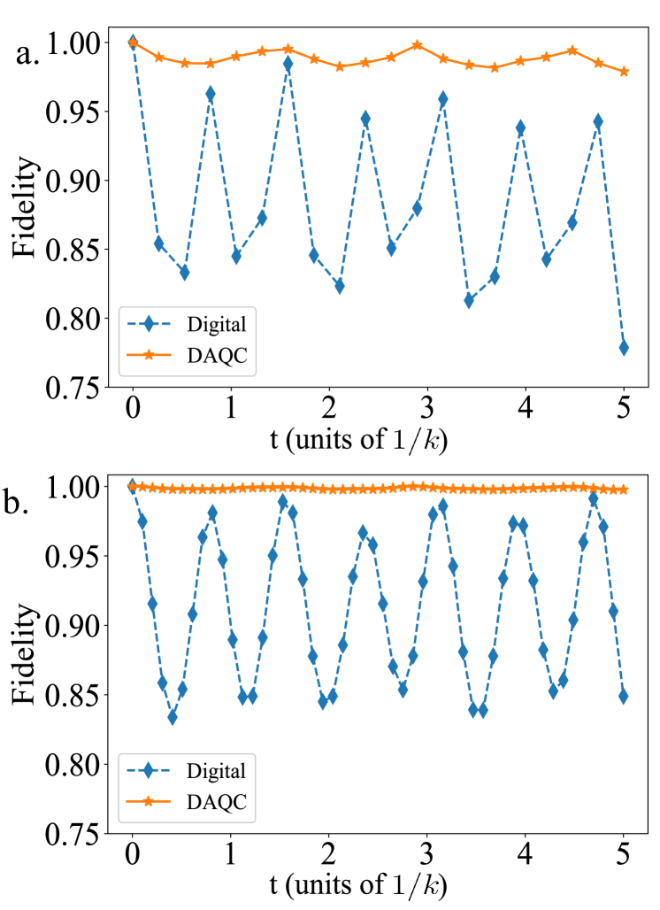
Figure 3: Fidelity, $\langle\psi_{exact}|\psi_{sim}\rangle^{2}$ as a function of time for a. 20, and b. 50 trotter steps with $k=1$, $g=k$, $U=2k$, and $\omega_{0}=8k$. The initial state is half-filling, $\psi_{i}=\left|{0,1,1,0,0,0}\right\rangle$. Each resonator was truncated to eight levels.

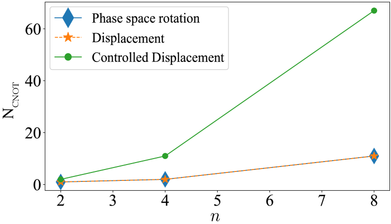
Figure 4: Number of CNOTs ($\rm{N_{CNOT}}$) required to perform each bosonic gate as a function of the number of levels ($n$) for each bosonic mode for a pure digital approach.

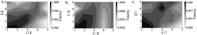
Figure 5: DAQC fidelity $\langle\psi_{exact}|\psi_{sim}\rangle$ as a function of different parameters for 50 trotter steps. The initial state is half-filling, $\psi_{i}=\left|{0,1,1,0,0,0}\right\rangle$, where each resonator was truncated to 8 levels.

Results.- For the simulation, we consider the dimensionless Hamiltonian $H/k$ and choose the timescale in units of $1/k$. For different materials, the range of parameters of the HH model Hamiltonian, Eq. (1) such as $k$ and $U$ lie between $0.2-10$ eV, $g$ is between $0-100$ eV and $\omega$ lies in the range $0.01-1$ eV [33], corresponding to which the physical timescale of the system is between $fs$ to $ps$. Considering the microwave driving with the qubit and resonator frequencies in the range $5-10$ GHz, the time for one trotter step for the digital blocks comprising the single and two-qubit gates are $10-500$ $ns$ [34] while for the analog blocks comprising the bosonic and qubit-bosonic gates are around $72$ $ns$ [32]. The initial states of the system are defined using the ordering of the Hilbert space as $\left|{Q_{1},Q_{2},Q_{3},Q_{4},res_{1},res_{2}}\right\rangle$, where $Q_{i}$ and $res_{i}$ denote the qubit and resonator subspaces, respectively.

We investigate the fidelity and dynamics of the system by varying the values of $g$, $U$, and $k$. Fig. 3 shows the fidelity of the DAQC and pure digital simulation with respect to the exact simulation with the system initialized at half-filling. Clearly, the DAQC simulation outperforms the pure digital computation, evidently displaying an enhanced performance.

The digital simulation was carried out using Bosonic Qiskit [35], where each resonator was truncated to $n$ levels. This requires an order of $\log_{2}n$ number of digital gates each, apart from the gates required for the qubits. The terms $a^{\dagger}a$, $a^{\dagger}+a$, and $\sigma_{z}(a^{\dagger}+a)$ can be implemented using cv_r$()$, cv_d$()$, and cv_c_d$()$ gates, respectively. This is provided by Bosonic Qiskit and corresponds to phase space rotation, displacement, and controlled displacement operators, respectively. When decomposed into digital gates, these bosonic gates can be realized using combinations of single qubit rotations $U3(\theta,\phi,\lambda)$ and CNOTs.

Since entangling gates are common in NISQ processors, we estimate the number of CNOTs required for each of these bosonic gates for a single trotter step. We plot the CNOTs required per bosonic gate with increasing resonator levels ($n$) in Fig. 4. The CNOTs required for the gates, cv_r$()$ and cv_d$()$, grow equally. In case of cv_c_d$()$, it grows with a very high margin requiring a total of 67 CNOTs for $n=8$.

From a dynamical point of view, our DAQC protocol can produce very high fidelities. For the two-site HH model, we compute the overlap between the exact solution and the numerical simulation using the DAQC protocol for different regimes as is shown in Fig. 5. We can observe that the fidelity is larger than 0.98, making our proposal suitable for studying dynamical condensed matter physics properties. Also, as the scaling of our proposal depends only on the smaller dimension of the lattice, we expect that these results can be maintained for larger systems.

Conclusions.- We developed a co-design DAQC approach for the quantum simulation strongly-correlated fermion-boson model in superconducting circuits. The proposed digital-analog encoding allows us to simulate the problem Hamiltonian with high fidelity and fewer resources as compared to the purely-digital case. We obtain a circuit-depth scaling proportional to $\ell^{2}$ for a $\ell\times h$ lattice where $\ell\leq h$. Such compact scaling cannot be obtained with purely-digital quantum computing, where the number of controlled gates and qubits grows with both dimensions in the lattice. Conversely, the scaling provided by other platforms like trapped ions grows with both dimensions, and does not have the versatility to encode several bosonic modes.

To demonstrate the performance of our model, we considered a 2-site Hubbard-Holstein model at half-filling. We benchmark the fidelity of the DAQC and digital simulation against the exact simulation, revealing high-fidelity values. Additionally, we explore the dynamics of the system, computing the fidelity with the exact evolution for different regimes, obtaining fidelities larger than 0.98 in all cases.

Our encouraging results suggest that these types of co-design encoding are suitable to outperform classical computation capabilities in the NISQ era, making our current quantum technology useful for industrial problems related to condensed-matter physics.

Acknowledgments.- We are thankful for the financial support of Agencia Nacional de Investigación y Desarrollo (ANID): Subvención a la Instalación en la Academia SA77210018, Fondecyt Regular 1231174, Financiamiento Basal para Centros Científicos y Tecnológicos de Excelencia AFB220001. We thank Prof. Lin Tian from University of California, Merced for important discussions regarding this project.

Appendix A Hamiltonian of the superconducting quantum simulator

In this section, we perform the circuit quantization of the superconducting architecture shown in Fig. 1 (d), for simulating the target Hamiltonian given in Eq. (2) of the main text. To do it more pedagogically, without loss of generality, we will focus in the description of the building block shown in Fig. 6, whose Lagrangian reads

$$\mathcal{L} =\sum_{j=1}^{2}\bigg{[}\frac{C_{g_{j}}}{2}(\dot{\Phi}_{j}-V_{g_{j}})^{2}+\frac{C_{J_{j}}}{2}\dot{\Phi}_{j}^{2}+E_{J_{j}}\cos{(\varphi_{j})}\bigg{]}+E_{J_{s}}^{\textrm{eff}}\cos{(\varphi_{s})}+\frac{C_{s}}{2}{\dot{\Phi}}_{s}^{2}+\frac{C_{c}}{2}(\dot{\Phi}_{1}-\dot{\Phi}_{s})^{2}+\frac{C_{c}}{2}(\dot{\Phi}_{s}-\dot{\Phi}_{2})^{2}$$ (15)

$$+\frac{C}{2}\dot{\Phi}_{R}^{2}+\frac{1}{2L}\Phi_{R}^{2}+\frac{C_{c}}{2}(\dot{\Phi}_{s}-\dot{\Phi}_{R})^{2},$$ (16)

where $\varphi_{j}=2\pi\Phi_{j}/\Phi_{0}$, with $\Phi_{0}=h/2e$ is the superconducting flux quantum and $2e$ is the electrical charge of a Cooper pair, and $E_{J_{s}}^{\textrm{eff}}=2E_{J_{s}}\cos{(\varphi_{ext})}$ is the effective Josephson energy of the SQUID. Now, we calculate the conjugate momenta (node charge) $Q_{j}=\partial L/\partial\dot{\Phi}_{j}$ obtaining

$$Q_{1(2)} = C_{g_{1(2)}}(\dot{\Phi}_{1(2)}-V_{g_{1(2)}})+C_{J_{1(2)}}\dot{\Phi}_{1(2)}+C_{c}(\dot{\Phi}_{1(2)}-\dot{\Phi}_{s})$$

$$Q_{s} = C_{s}\dot{\Phi}_{s}-C_{c}(\dot{\Phi}_{1}-\dot{\Phi}_{s})-C_{c}(\dot{\Phi}_{2}-\dot{\Phi}_{s})+C_{c}(\dot{\Phi}_{s}-\dot{\Phi}_{R})$$

$$Q_{R} = C\dot{\Phi_{R}}-C_{c}(\dot{\Phi}_{s}-\dot{\Phi}_{R}),$$ (17)

The classical Hamiltonian is obtained by applying the Legendre transformation $\mathcal{H}(\Phi_{k},Q_{k})=\vec{Q}^{\top}_{k}\vec{\dot{\Phi}}_{k}-\mathcal{L}$, obtaining

$$\mathcal{H}=\sum_{j=1}^{2}\bigg{[}\frac{1}{2\tilde{C}_{j}}(Q_{j}+\tilde{Q_{j}})^{2}-E_{J_{j}}\cos{(\varphi_{j})}\bigg{]}+\bigg{[}\frac{1}{2C_{7}}Q_{s}^{2}-E_{J_{s}}^{\textrm{eff}}\cos{(\varphi_{s})}+\frac{1}{2C_{9}}Q_{R}^{2}+\frac{1}{2L}\Phi_{R}^{2}\bigg{]}+\frac{1}{2}\bigg{[}\frac{2}{C_{2}}Q_{1}Q_{2}+\frac{2}{C_{3}}Q_{1}Q_{s}+\frac{2}{C_{5}}Q_{2}Q_{s}\\ +\frac{2}{C_{4}}Q_{1}Q_{R}+\frac{2}{2C_{6}}Q_{2}Q_{R}+\frac{2}{C_{8}}Q_{R}Q_{s}+\frac{2}{C_{2}}\tilde{Q_{1}}Q_{2}+\frac{2}{C_{2}}Q_{1}\tilde{Q_{2}}+\frac{2}{C_{2}}\tilde{Q_{1}}\tilde{Q_{2}}+\frac{2}{C_{3}}\tilde{Q_{1}}Q_{s}+\frac{2}{C_{4}}\tilde{Q_{1}}Q_{R}+\frac{2}{C_{5}}\tilde{Q_{2}}Q_{s}+\frac{2}{C_{6}}\tilde{Q_{2}}Q_{R}\bigg{]}$$ (18)

where, $\tilde{C}_{1}={\tilde{S}_{c}}/{\left[\tilde{C}\left(\tilde{C}_{s}C_{\Sigma 2}-C_{c}^{2}\right)-C_{c}^{2}C_{\Sigma 2}\right]}$, $\tilde{C}_{2}={\tilde{S}_{c}}/\left[\tilde{C}\left(\tilde{C}_{s}C_{\Sigma 1}-C_{c}^{2}\right)-C_{c}^{2}C_{\Sigma 1}\right]$, $C_{2}={\tilde{S}_{c}}/C_{c}^{2}\tilde{C}$, $C_{3}={\tilde{S}_{c}}/\tilde{C}C_{c}C_{\Sigma 2}$, $C_{4}={\tilde{S}_{c}}/C_{c}^{2}C_{\Sigma 2}$, $C_{5}={\tilde{S}_{c}}/\tilde{C}C_{c}C_{\Sigma 1}$, $C_{6}={\tilde{S}_{c}}/C_{c}^{2}C_{\Sigma 1}$, $C_{7}={\tilde{S}_{c}}/\tilde{C}C_{\Sigma 1}C_{\Sigma 2}$, $C_{8}={\tilde{S}_{c}}/C_{c}C_{\Sigma 1}C_{\Sigma 2}$, $C_{9}={\tilde{S}_{c}}/\left[C_{\Sigma 2}\left(\tilde{C}_{s}C_{\Sigma 1}-C_{c}^{2}\right)-C_{c}^{2}C_{\Sigma 1}\right]$, $\tilde{Q_{1}}=C_{g_{1}}V_{g_{1}}$ and $\tilde{Q_{2}}=C_{g_{2}}V_{g_{2}}$, and $C^{-1}$ is the inverse capacitance matrix. The offset terms have been neglected.

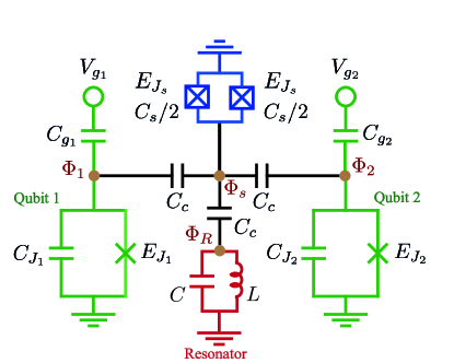
Figure 6: Superconducting building-block architecture for emulating the H-H model.

Using the approximations, $\dot{\Phi}_{s}\ll\dot{\Phi}_{1(2)}$ and ${\Phi}_{s}\ll{\Phi}_{1(2)}$, i.e. we consider the SQUID in the high plasma frequency regime, and low impedance. From the first approximation $\dot{\Phi}_{s}\ll\dot{\Phi}_{1(2)}$, we can approximate $\dot{\Phi}_{1(2)}-\dot{\Phi}_{s}\approx\dot{\Phi}_{1(2)}$ and since $C_{s}\sim C_{g_{1(2)}}$, we can approximate $C_{c}\dot{\Phi}_{1(2)}-C_{s}\dot{\Phi}_{s}\approx C_{c}\dot{\Phi}_{1(2)}$ in Eq. (17), obtaining

$$Q_{s}=-C_{c}\bigg{(}\frac{Q_{1}+\tilde{Q}_{1}}{C_{\sum_{1}}}+\frac{Q_{2}+\tilde{Q}_{2}}{C_{\sum_{2}}}+\frac{Q_{R}}{C+C_{c}}\bigg{)}$$ (19)

where, $\tilde{Q}_{j}=C_{g_{j}}V_{g_{j}}$. Using the Euler-Lagrange equation $\frac{d}{dt}\bigg{(}\frac{\partial{\mathcal{L}}}{\partial{\dot{\Phi}}}\bigg{)}-\frac{\partial{\mathcal{L}}}{\partial{\Phi}}=0$, we obtain the relations

$${C_{g_{1(2)}}}\ddot{\Phi}_{1(2)}+{C_{J_{1(2)}}}\ddot{\Phi}_{1(2)}+\frac{2\pi}{\Phi_{0}}E_{J_{j}}\sin{(\varphi_{j})}+{C_{c}}(\ddot{\Phi}_{1(2)}-\ddot{\Phi}_{s})=0$$

$$C_{s}\ddot{\Phi}_{s}+C_{c}(-\ddot{\Phi}_{1}-\ddot{\Phi}_{2}-\ddot{\Phi}_{R}+3\ddot{\Phi}_{s})+\frac{2\pi}{\Phi_{0}}E_{J_{s}}^{\textrm{eff}}\sin{\varphi_{s}}=0$$

$$C\ddot{\Phi}_{R}+C_{c}(\ddot{\Phi}_{R}-\ddot{\Phi}_{s})-\frac{\Phi_{R}}{L}=0$$ (20)

where, we have used $\varphi_{j}=2\pi\Phi_{j}/\Phi_{0}$. Considering the mentioned approximations, we obtain

$$\varphi_{s}=\frac{C_{c}}{E_{J_{s}}^{\textrm{eff}}}\bigg{(}-\frac{E_{J_{1}}\sin\varphi_{1}}{C_{g1}+C_{j1}+C_{c}}-\frac{E_{J_{2}}\sin\varphi_{2}}{C_{g2}+C_{j2}+C_{c}}+\frac{\Phi_{0}}{2\pi}\frac{\Phi_{R}}{L(C+Cc)}\bigg{)}$$ (21)

Using Eq. (19) and Eq. (21) in Eq. (18) we get

$$\mathcal{H} =\sum_{j=1}^{2}\bigg{[}\frac{1}{2\bar{C}_{j}}(Q_{j}+\tilde{Q_{j}})^{2}-E_{J_{j}}\cos{(\varphi_{j})}+\frac{E_{J_{s}}^{\textrm{eff}}}{2}\gamma_{j}^{2}(\varphi_{ext})(\sin\varphi_{j})^{2}-\gamma_{j}(\varphi_{ext})\sin\varphi_{j}\frac{\Phi_{0}\Phi_{R}}{2\pi L(\frac{C}{C_{c}}+1)}\bigg{]}+\bigg{[}\frac{1}{2\bar{C}_{R}}{Q_{R}}^{2}+\frac{1}{2L}\Phi_{R}^{2}$$ (22)

$$+\frac{1}{2E_{J_{s}}^{\textrm{eff}}}\frac{\Phi_{0}^{2}\Phi_{R}^{2}}{4\pi^{2}L^{2}(\frac{C}{C_{c}}+1)^{2}}+E_{J_{s}}^{\textrm{eff}}\gamma_{1}\gamma_{2}(\varphi_{ext})\sin\varphi_{1}\sin\varphi_{2}\bigg{]}$$ (23)

where, $\bar{C}_{j}=\tilde{C}_{j}+\frac{\tilde{S}_{c}C_{\sum_{j}}}{C_{c}^{2}{C}_{\sum_{3-j}}}$, $\bar{C}_{R}=C_{7}({\frac{C}{C_{c}}+1})^{2}-\frac{C_{8}(C+C_{c})}{2C_{c}}$ and $\gamma_{j}=\frac{E_{J_{j}}}{(E_{J_{s}}^{\textrm{eff}})(\frac{C_{gj}}{C_{c}}+\frac{C_{J_{j}}}{C_{c}}+1)}$. where we also consider $\cos\varphi_{s}=(1-\varphi_{s}^{2}/2)$.

Promoting the variables to the quantum operators by the transformations, $Q_{j}\rightarrow\hat{Q}_{j}=2e\hat{n}_{j}$, $\varphi_{j}\rightarrow\hat{\varphi}_{j}$, $Q_{R}\rightarrow\hat{Q}_{R}=2e\hat{n}_{R}$ and $\Phi_{R}\rightarrow\hat{\Phi}_{R}$ with the commutation relations $[\hat{\Phi}_{j},\hat{Q}_{j}]=i\hbar$ and $[\hat{\Phi}_{R},\hat{Q}_{R}]=i\hbar$, where the factor 2 in the charge operators corresponds to the cooper pairs, we can write

$$\mathcal{H} =\sum_{j=1}^{2}\bigg{[}4E_{\tilde{C}_{j}}(\hat{n}_{j}-\bar{n}_{g})^{2}-E_{J_{j}}\cos{(\hat{\varphi}_{j})}+\frac{E_{J_{s}}^{\textrm{eff}}}{2}\gamma_{j}^{2}(\varphi_{ext})(\sin\hat{\varphi}_{j})^{2}-\frac{\hat{\Phi}_{0}^{2}}{4\pi^{2}}\gamma_{j}(\varphi_{ext})\sin\hat{\varphi}_{j}\frac{\hat{\varphi}_{R}}{L(\frac{C}{C_{c}}+1)}\bigg{]}+\bigg{[}{4E_{C_{R}}\hat{n}_{R}}^{2}$$ (24)

$$+\frac{E_{L_{R}}}{2}\hat{\varphi}_{R}^{2}+\frac{E_{L_{S}}(\varphi_{ext})}{2}\hat{\varphi}_{R}^{2}+E_{J_{s}}^{\textrm{eff}}\gamma_{1}\gamma_{2}(\varphi_{ext})\sin\hat{\varphi}_{1}\sin\hat{\varphi}_{2}\bigg{]}$$ (25)

where, $E_{C_{R}}={e}^{2}/{2\bar{C}_{R}}$, $E_{L_{R}}=\bigg{(}\frac{\Phi_{0}}{2\pi}\bigg{)}^{2}/{L}$ and $E_{L_{S}}=\bigg{(}\frac{\Phi_{0}}{2\pi}\bigg{)}^{2}/L_{S}{(\varphi_{ext})}$. We rewrite the Hamiltonian in the number basis, it means, $\hat{n}_{j}=\sum_{m}\left|{m_{j}}\right\rangle\left\langle{m_{j}}\right|$, $\cos(\hat{\varphi}_{j})=\frac{1}{2}(\sum_{m}\left|{m_{j}}\right\rangle\left\langle{m_{j}+1}\right|+H.C)$, $\sin(\hat{\varphi}_{j})=-\frac{i}{2}(\sum_{m}\left|{m_{j}}\right\rangle\left\langle{m_{j}+1}\right|-H.C)$, Also, for the LC resonator we can define annihilation ($a$) and creation ($a^{\dagger}$) operators as $\hat{n}_{R}=in_{R}(\hat{a}^{\dagger}-\hat{a})$ and $\hat{\varphi}_{R}=\phi_{R}(\hat{a}^{\dagger}+\hat{a})$, where, $n_{j}=(E_{J_{j}}/32E_{\tilde{C}_{j}})^{1/4}$, $\varphi_{j}=(2E_{\tilde{C}_{j}}/E_{J_{j}})^{1/4}$, $n_{R}=(E_{L_{R}}/32E_{C_{R}})^{1/4}$ and $\phi_{R}=(2E_{C_{R}}/E_{L_{R}})^{1/4}$. Finally, by performing the two-level approximation for the transmon degrees of freedom

$$\sin(\varphi_{j})=\frac{1}{2}\sigma_{j}^{y},\;\;\;\gamma_{j}^{2}(\varphi_{ext})(\sin\hat{\varphi}_{j})^{2}=\gamma_{j}^{2}/4$$ (26)

where, $\sigma_{j}^{y}$ is the Pauli Y matrix. Since $\gamma_{j}^{2}(\varphi_{ext})(\sin\hat{\varphi}_{j})^{2}$ is a constant term, we can ignore it as it only provides a shift to the qubit frequency. Using these relations, the Hamiltonian is given by

$$\mathcal{\hat{H}}=\sum_{j=1}^{2}\bigg{[}\frac{\omega_{j}}{2}\sigma_{j}^{z}-\frac{\omega^{\prime}_{j}(\varphi_{ext})}{2}\sigma_{j}^{y}{(\hat{a}^{\dagger}+\hat{a})}\bigg{]}+\bigg{[}{\omega_{R}\bigg{(}a^{\dagger}a}+\frac{1}{2}\bigg{)}+\frac{E_{L_{S}}(\varphi_{ext})}{2}\phi_{R}(\hat{a}^{\dagger}+\hat{a})^{2}+\frac{E_{J_{s}}^{\textrm{eff}}\gamma_{1}\gamma_{2}(\varphi_{ext})}{4}\sigma_{1}^{y}\sigma_{2}^{y}\bigg{]}$$

(27)

where, $\omega_{j}=\sqrt{8E_{\tilde{C}_{j}}E_{J_{j}}}$, $\omega_{j}^{\prime}(\varphi_{ext})=\frac{\hat{\Phi}_{0}^{2}}{4\pi^{2}}\gamma_{j}(\varphi_{ext})\frac{{\phi}_{R}}{L(\frac{C}{C_{c}}+1)}$ and $\omega_{R}=\sqrt{8E_{L_{R}}E_{C_{R}}}$. We consider the external flux to be composed of a DC signal and a small AC signal, $\varphi_{ext}=\varphi_{DC}+\varphi_{AC}(t)$, where $\varphi_{AC}(t)=\varphi_{R}+\sum_{\alpha}\varphi_{QQ}^{\alpha}+\varphi_{QR}^{\alpha(1)}+\varphi_{QR}^{\alpha(2)}$, where $\alpha=\{+,-\}$ and $\varphi_{ab}^{\alpha}=A_{ab}\cos(\nu_{ab}^{\alpha}t+\tilde{\varphi}_{ab}^{\alpha})$. Furthermore, for the case $|A_{i}|\ll 1$, we can approximate

$$\frac{1}{E_{J_{s}}^{\textrm{eff}}}\approx\frac{1}{\bar{E}_{J_{s}}}\bigg{[}1+\frac{\sin(\varphi_{DC})}{\cos{\varphi_{DC}}}\varphi_{AC}(t)\bigg{]}$$ (28)

where, $\bar{E}_{J_{s}}=2E_{J_{s}}\cos\varphi_{DC}$. Using the Eq. (28) in the Eq. (27), we get

$$\mathcal{\hat{H}}=\bigg{[}\frac{\omega_{1}}{2}\sigma_{1}^{z}+\frac{\omega_{2}}{2}\sigma_{2}^{z}+{\omega_{R}\bigg{(}a^{\dagger}a}+\frac{1}{2}\bigg{)}\bigg{]}+\bigg{[}[k_{0}+k_{1}\varphi_{AC}(t)](\hat{a}^{\dagger}+\hat{a})^{2}+{[m_{0}+m_{1}\varphi_{AC}(t)]}\sigma_{1}^{y}\sigma_{2}^{y}-\sum_{j=1}^{2}[{l_{0}^{j}+l_{1}^{j}\varphi_{AC}(t)}]\sigma_{j}^{y}{(\hat{a}^{\dagger}+\hat{a})}\bigg{]}$$ (29)

where the coupling strengths are defined as

$$k_{0} =\frac{\phi_{R}}{\bar{E}_{J_{S}}}\bigg{(}\frac{\Phi_{0}^{2}}{4\pi^{2}L(C/C_{c}+1)}\bigg{)}^{2},m_{0}=\frac{1}{4\bar{E}_{J_{s}}}\frac{E_{J_{1}}E_{J_{2}}}{\bigg{(}\frac{C_{gj}}{C_{c}}+\frac{C_{J_{j}}}{C_{c}}+1\bigg{)}},l_{0}^{j}=\frac{\Phi_{0}^{2}}{4\pi^{2}\bar{E}_{J_{s}}}\frac{\phi_{R}}{L\bigg{(}\frac{C}{C_{c}}+1\bigg{)}}\frac{E_{J_{j}}}{\bigg{(}\frac{C_{gj}}{C_{c}}+\frac{C_{J_{j}}}{C_{c}}+1\bigg{)}},$$

$$k_{1}=k_{0}\tan(\varphi_{DC}),\;\;\;m_{1}=m_{0}\tan(\varphi_{DC}),\;\;\;l_{1}^{j}=l_{0}^{j}\tan(\varphi_{DC})$$ (30)

With current state-of-the-art superconducting technologies [34] we can achieve the range $0\leq l_{1}^{j}/g_{0}\leq 6.8$. The parameter ranges for various components correspond to $C\approx 15-40fF$, $C_{c}=C_{g}=0.1C$ for the capacitors and coupling (or gate) capacitors, $L\approx nH$, for the inductors, $E_{J}=E_{Js}\approx 10E_{c}-50E_{c}$ for the qubit and SQUID Josephson energies. To get the effective intereaccions, we can write the Hamiltonian in the interaction picture, considering as free Hamiltonian $\mathcal{H}_{0}=\bigg{[}\frac{\omega_{1}}{2}\sigma_{1}^{z}+\frac{\omega_{2}}{2}\sigma_{2}^{z}+{\omega_{R}\bigg{(}a^{\dagger}a}+\frac{1}{2}\bigg{)}\bigg{]}$ and the interaction as $V=\bigg{[}[k_{0}+k_{1}\varphi_{AC}(t)](\hat{a}^{\dagger}+\hat{a})^{2}+{[m_{0}+m_{1}\varphi_{AC}(t)]}\sigma_{1}^{y}\sigma_{2}^{y}-\frac{1}{4}\sum_{j=1}^{2}[{l_{0}^{j}+l_{1}^{j}\varphi_{AC}(t)}]\sigma_{j}^{y}{(\hat{a}_{j}^{\dagger}+\hat{a}_{j})}\bigg{]}$. Finally we choose $\nu_{QQ}^{\pm}=\omega_{1}\pm\omega_{2}$, $\nu_{QR}^{\pm(1)}=\omega_{1}\pm\omega_{R}$, $\nu_{QR}^{\pm(2)}=\omega_{2}\pm\omega_{R}$, and after a rotating wave approximation, neglecting the fast oscillation terms, we obtain the final effective Hamiltonian for each building block (site)

$$H_{s} =\frac{m_{1}A_{QQ}}{4}\Big{[}C_{QQ}^{+}\sigma_{L,j}^{x}\sigma_{R,j}^{x}-S_{QQ}^{+}\sigma_{L,j}^{x}\sigma_{R,j}^{y}+S_{QQ}^{-}\sigma_{L,j}^{y}\sigma_{R,j}^{x}+C_{QQ}^{-}\sigma_{L,j}^{y}\sigma_{R,j}^{y}\Big{]}$$

$$+\frac{1}{4}\sum_{\alpha=\{L,R\}}A_{QR}l_{1}^{\alpha}\Big{[}C_{QR}^{+}\sigma_{\alpha,j}^{x}(a_{j}^{\dagger}-a_{j})-C_{QR}^{-}\sigma_{\alpha,j}^{y}(a_{j}^{\dagger}+a_{j})+S_{QR}^{+}\sigma_{\alpha,j}^{x}(a_{j}^{\dagger}+a_{j})-S_{QR}^{-}\sigma_{\alpha,j}^{y}(a_{j}^{\dagger}-a_{j})\Big{]},$$

we have replaced the index $1(2)\rightarrow L(R)$ to refer to the qubit left and right of each building block. Also we have defined $C_{ab}^{\pm}=\cos\tilde{\varphi}_{ab}^{+}\pm\cos\tilde{\varphi}_{ab}^{-}$, and a similar definitions for $S_{ab}^{\pm}$ by replacing $\sin$ by $\cos$. We compare the dynamics of the Schrödinger and Interaction picture Hamiltonians in the plots shown in Fig. 7. The results of the population of states and the dynamics of the Pauli $\sigma_{z}$ operator of both pictures coincide well.

Following the same procedure we can derive the Hamiltonian to couple adjacent building blocks which reads

$$H_{s-s}^{(j)}=\frac{m_{1}\bar{A}_{QQ}}{4}\Big{[}C_{\phi QQ}^{+}\sigma_{R,j}^{x}\sigma_{L,j+1}^{x}-S_{\phi QQ}^{+}\sigma_{R,j}^{x}\sigma_{L,j+1}^{y}+S_{\phi QQ}^{-}\sigma_{R,j}^{y}\sigma_{L,j+1}^{x}+C_{\phi QQ}^{-}\sigma_{R,j}^{y}\sigma_{L,j+1}^{y}\Big{]}$$ (32)

where $\tilde{C}_{ab}^{\pm}=\cos\tilde{\phi}_{ab}^{+}\pm\cos\tilde{\phi}_{ab}^{-}$, and $S_{ab}^{\pm}$ is obtained by replacing $\sin$ by $\cos$.

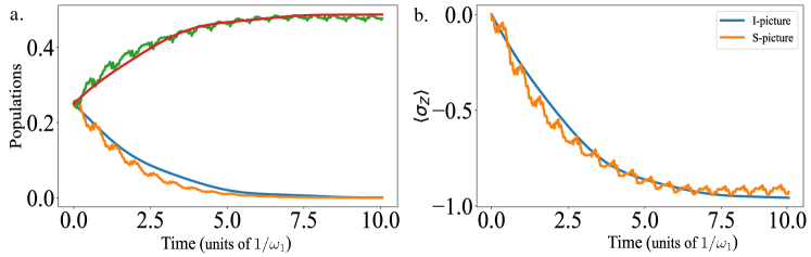
Figure 7: We compare the curves corresponding to the effective dynamics given by Hamiltonian in Eq. (LABEL:B19) and exact dynamics. a. Population of states $\left|{000}\right\rangle$ (orange) and $\left|{001}\right\rangle$ (green). b. Dynamics of $\langle\sigma_{z}\rangle$, initial state $\left|{\psi}\right\rangle=\left|{\psi_{1}}\right\rangle\otimes\left|{\psi_{r}}\right\rangle\otimes\left|{\psi_{2}}\right\rangle$, where $\left|{\psi_{i}}\right\rangle=\frac{1}{\sqrt{2}}\big{(}\left|{0}\right\rangle+\left|{1}\right\rangle\big{)}$ are the initial qubit states and $\left|{\psi_{r}}\right\rangle=\left|{0}\right\rangle$ is the initial state of the resonator. We use $k_{0}=0.08$, $l_{0}=0.02$ and $m_{0}=0.01$, $A_{i}/\varphi_{DC}=0.1$, $\omega_{1}=1$, $\omega_{2}=0.9$ and $\omega_{R}=0.6$ (frequencies are in units of 1/$\omega_{1}$), and the phases are $\tilde{\varphi}_{QQ}^{\pm}=\pi$, $\tilde{\varphi}_{QR}^{\pm(j)}=0$.

Operator					$\tilde{\varphi}_{QQ}^{+}$					$\tilde{\varphi}_{QQ}^{-}$					$\tilde{\varphi}_{QR}^{+(L)}$					$\tilde{\varphi}_{QR}^{-(L)}$					$\tilde{\varphi}_{QR}^{+(R)}$					$\tilde{\varphi}_{QR}^{-(R)}$
$\sigma_{L,j}^{x}\sigma_{R,j}^{x}$					0					0					——-					——-					——-					——-
$\sigma_{L,j}^{y}\sigma_{R,j}^{y}$					0					$\pi$					——-					——-					——-					——-
$\sigma_{L,j}^{x}\sigma_{R,j}^{y}$					$\pi/2$					$-\pi/2$					——-					——-					——-					——-
$\sigma_{L,j}^{y}\sigma_{R,j}^{x}$					$\pi/2$					$\pi/2$					——-					——-					——-					——-
$\sigma_{L,j}^{x}(a+a^{\dagger})$					——-					——-					$\pi/2$					$\pi/2$					——-					——-
$\sigma_{R,j}^{x}(a+a^{\dagger})$					——-					——-					——-					——-					$\pi/2$					$\pi/2$
$\sigma_{L,j}^{y}(a+a^{\dagger})$					——-					——-					$-\pi/2$					$\pi/2$					——-					——-
$\sigma_{R,j}^{y}(a+a^{\dagger})$					——-					——-					——-					——-					$-\pi/2$					$\pi/2$
$\sigma_{L,j}^{x}(a-a^{\dagger})$					——-					——-					0					0					——-					——-
$\sigma_{R,j}^{x}(a-a^{\dagger})$					——-					——-					——-					——-					0					0
$\sigma_{L,j}^{y}(a-a^{\dagger})$					——-					——-					$\pi$					0					——-					——-
$\sigma_{R,j}^{y}(a-a^{\dagger})$					——-					——-					——-					——-					$\pi$					0

Table 1: Phase selection to mimic different interactions.

References

• [1] E. Berger, P. Valás̆ek, and W. von der Linden, Two-dimensional Hubbard-Holstein model, Phys. Rev. B, 52, 4806 (1995).
• [2] G. Wellein, H. Röder, and H. Fehske, Polarons and bipolarons in strongly interacting electron-phonon systems, Phys. Rev. B 53, 9666 (1996).
• [3] G. De Filippis, V. Cataudella, G. Iadonisi, V. Marigliano Ramaglia, C. A. Perroni, and F. Ventriglia, Polaron and bipolaron formation in the Hubbard-Holstein model: Role of next-nearest-neighbor electron hopping, Phys. Phys. Rev. B 64, 155105 (2001).
• [4] P. Werner, and M. Eckstein, Field-induced polaron formation in the Holstein-Hubbard model, EPL 109, 37002 (2016).
• [5] L. Friedman, Electron-Phonon Interaction in Organic Molecular Crystals, Phys. Rev. 140, A1649 (1965).
• [6] Y. Dahnovskya, Ab initio electron propagators in molecules with strong electron-phonon interaction. I. Phonon averages, Nat. Rev. Phys. 2, 499 (2020).
• [7] F. Novelli et. al, Witnessing the formation and relaxation of dressed quasi-particles in a strongly correlated electron system, Nat Commun 5, 5112 (2014).
• [8] T. P. Devereaux, T. Cuk, Z.-X. Shen, and N. Nagaosa, Anisotropic Electron-Phonon Interaction in the Cuprates, Phys. Rev. Lett. 93, 117004 (2004).
• [9] V. L. Aksenov, and V. V. Kabanov, Electron-phonon interaction and Raman linewidth in superconducting fullerides, Phys. Rev. B. 57, 608 (1998).
• [10] V. Esposito et. al, Nonlinear Electron-Phonon Coupling in Doped Manganites, Phys. Rev. Lett. 118, 247601 (2017).
• [11] C. A. Jimínez-Hoyos and G. E. Scuseria, Cluster-based mean-field and perturbative description of strongly correlated fermion systems: Application to the one- and two-dimensional Hubbard model, Phys. Rev. B 92, 085101 (2015).
• [12] G. S. Jeon, T.-H. Park, J. H. Han, H. C. Lee, and H.-Y. Choi, Dynamical mean-field theory of the Hubbard-Holstein model at half filling: Zero temperature metal-insulator and insulator-insulator transitions, Phys. Rev. B 70, 125114 (2004).
• [13] S. Backes, Y. Murakami, S. Sakai, and R. Arita, Dynamical mean-field theory for the Hubbard-Holstein model on a quantum device, Phys. Rev. B 107, 165155 (2023).
• [14] S. Johnston, E. A. Nowadnick, Y. F. Kung, B. Moritz, R. T. Scalettar, and T. P. Devereaux, Determinant quantum Monte Carlo study of the two-dimensional single-band Hubbard-Holstein model, Phys. Rev. B 87, 235133 (2013).
• [15] N. C. Costa, K. Seki, S. Yunoki, and S. Sorella, Phase diagram of the two-dimensional Hubbard-Holstein model, Commun. Phys. 3, 80 (2020).
• [16] F. Malet, A. Mirtschink, C. B. Mendl, J. Bjerlin, E. Ö. Karabulut, S. M. Reimann, and P. Gori-Giorgi, Density-Functional Theory for Strongly Correlated Bosonic and Fermionic Ultracold Dipolar and Ionic Gases, Phys. Rev. Lett 115, 033006 (2015).
• [17] P. Corboz, R. Orús, B. Bauer, and G. Vidal, Simulation of strongly correlated fermions in two spatial dimensions with fermionic projected entangled-pair states, Phys. Rev. Lett 81, 165104 (2010).
• [18] E. Jeckelmann and S. R. White, Density-matrix renormalization-group study of the polaron problem in the Holstein model, Phys. Rev. B 57, 6376 (1998).
• [19] I.M. Georgescu, S. Ashhab, and F. Nori, Quantum simulation, Rev. Mod. Phys. 86, 153 (2014).
• [20] D. Lv, S. An, Z. Liu, J.-N. Zhang, J. S. Pedernales, L. Lamata, E. Solano, and K. Kim, Quantum Simulation of the Quantum Rabi Model in a Trapped Ion, Phys. Rev. X 8, 021027 (2018).
• [21] J. S. Pedernales, I. Lizuain, S. Felicetti, G. Romero, L. Lamata, and E. Solano, Quantum Rabi Model with Trapped Ions, Phys. Rev. B 88, 224502 (2013).
• [22] F. Mei, V. M. Stojanović, I. Siddiqi, and L. Tian, Analog superconducting quantum simulator for Holstein polarons, Sci. Rep. 5, 15472 (2015).
• [23] A. Parra-Rodriguez, P. Lougovski, L. Lamata, E. Solano, and M. Sanz Digital-analog quantum computations, Phys. Rev. A 101, 022305 (2020).
• [24] A. Mezzacapo, J. Casanova, L. Lamata, and E. Solano, Digital Quantum Simulation of the Holstein Model in Trapped Ions, Phys. Rev. Lett. 109, 200501 (2012).
• [25] J. P. Hague, and C. MacCormick, Quantum simulation of electron-phonon interactions in strongly deformable materials, New J. Phys. 14, 033019 (2012).
• [26] L. Tarruell, L. Sanchez-Palencia, Quantum simulation of the Hubbard model with ultracold fermions in optical lattices, Comptes Rendus Physique. 19, 6 (2018).
• [27] L. García-Álvarez, U. Las Heras, A. Mezzacapo, M. Sanz, E. Solano, and L. Lamata, Quantum chemistry and charge transport in biomolecules with superconducting circuits, Sci. Rep. 6, 27836 (2016).
• [28] U. Las Heras, L. García-Alvarez, A. Mezzacapo, E. Solano and L. Lamata, Fermionic models with superconducting circuits, EPJ Quantum Technol. 2, 8 (2015).
• [29] J. Yu, J. C. Retamal, M. Sanz, E. Solano, and F. Albarrán-Arriagada, Superconducting circuit architecture for digital-analog quantum computing, EPJ Quantum Technol. 9, 9 (2022).
• [30] P. Jordan, and E. Wigner , Über das Paulische Äquivalenzverbot, Z. Physik. 47, 631–651 (1928).
• [31] S. McArdle, S. Endo, A. Aspuru-Guzik, S. C. Benjamin, and X. Yuan, Quantum computational chemistry, Rev. Mod. Phys. 92, 015003 (2020).
• [32] C. S. Wang et.al, Efficient Multiphoton Sampling of Molecular Vibronic Spectra on a Superconducting Bosonic Processor, Phys. Rev. X. 10, 021060 (2020).
• [33] S. Pradhan and G. V. Pai Holstein-Hubbard model at half filling: A static auxiliary field study, Phys. Rev. B. 92, 165124 (2015).
• [34] G. Wendin, Quantum information processing with superconducting circuits: a review, Rep. Prog. Phys. 80 (2017).
• [35] T. J. Stavenger, E. Crane, K. C. Smith, C. T. Kang, S. M. Girvin, and N. Wiebe C2QA - Bosonic Qiskit, arXiv:2209.11153v2 (2022).