Dual-Balancing for Multi-Task Learning

Abstract

Multi-task learning (MTL), a learning paradigm to learn multiple related tasks simultaneously, has achieved great success in various fields. However, task balancing problem remains a significant challenge in MTL, with the disparity in loss/gradient scales often leading to performance compromises. In this paper, we propose a Dual-Balancing Multi-Task Learning (DB-MTL) method to alleviate the task balancing problem from both loss and gradient perspectives. Specifically, DB-MTL ensures loss-scale balancing by performing a logarithm transformation on each task loss, and guarantees gradient-magnitude balancing via normalizing all task gradients to the same magnitude as the maximum gradient norm. Extensive experiments conducted on several benchmark datasets consistently demonstrate the state-of-the-art performance of DB-MTL.

1 Introduction

Multi-task learning (MTL) (Caruana, 1997, Zhang & Yang, 2022) jointly learns multiple related tasks using a single model, improving parameter-efficiency and inference speed compared with learning a separate model for each task. By sharing the model, MTL can extract common knowledge to improve each task’s performance. MTL has demonstrated its superiority in various fields, such as computer vision (Liu et al., 2019a, Vandenhende et al., 2020; 2021, Xu et al., 2022, Ye & Xu, 2022), natural language processing (Liu et al., 2017; 2019b, Sun et al., 2020, Chen et al., 2021, Wang et al., 2021), and recommendation systems (Ma et al., 2018a; b, Tang et al., 2020, Hazimeh et al., 2021, Wang et al., 2023).

To learn multiple tasks simultaneously, equal weighting (EW) (Zhang & Yang, 2022) is a straightforward method that minimizes the sum of task losses with equal task weights but usually causes the challenging task balancing problem (Vandenhende et al., 2021, Lin et al., 2022), where some tasks perform well but the others perform unsatisfactorily (Standley et al., 2020). A number of methods have been recently proposed to alleviate this problem by dynamically tune the task weights. They can be roughly categorized into loss balancing methods (Kendall et al., 2018, Liu et al., 2019a; 2021b, Ye et al., 2021) such as balancing tasks based on learning speed (Liu et al., 2019a) or validation performance (Ye et al., 2021) at the loss level, and gradient balancing approaches (Chen et al., 2018b, Sener & Koltun, 2018, Chen et al., 2020, Yu et al., 2020, Liu et al., 2021a; b, Wang et al., 2021, Navon et al., 2022, Fernando et al., 2023) such as balancing gradients by mitigating gradient conflicts (Yu et al., 2020) or enforcing gradient norms close (Chen et al., 2018b) at the gradient level. Recently, Lin et al. (2022), Kurin et al. (2022), Xin et al. (2022) conduct extensive empirical studies and demonstrate that the performance of existing methods are undesirable, which indicates the task balancing issue is still an open problem in MTL.

In this paper, we focus on simultaneously balancing loss scales at the loss level and gradient magnitudes at the gradient level to mitigate the task balancing problem. Since the loss scales/gradient magnitudes among tasks can be different, a large one can dominate the update direction of the model, causing unsatisfactory performance on some tasks (Standley et al., 2020, Liu et al., 2021b). Therefore, we propose a simple yet effective Dual-Balancing Multi-Task Learning (DB-MTL) method that consists of loss-scale and gradient-magnitude balancing approaches. First, we perform a logarithm transformation on each task loss to ensure all task losses have the same scale, which is non-parametric and can recover the loss transformation in IMTL-L (Liu et al., 2021b). We find that the logarithm transformation also benefits the existing gradient balancing methods, as shown in Figure 1. Second, we normalize all task gradients to the same magnitude as the maximum gradient norm, which is training-free and guarantees all gradients’ magnitude are the same compared with GradNorm (Chen et al., 2018b). We empirically find that the magnitude of normalized gradients plays an important role in performance and setting it as the maximum gradient norm among tasks performs the best, as shown in Figure 4, thus it is adopted. We perform extensive experiments on several benchmark datasets and the results consistently demonstrate DB-MTL achieves state-of-the-art performance.

Our contributions are summarized as follows: (i) We propose the DB-MTL method, a dual-balancing approach to alleviate the task-balancing problem, consisting of loss-scale and gradient-magnitude balancing methods; (ii) We conduct extensive experiments to demonstrate that DB-MTL achieves state-of-the-art performance on several benchmark datasets; (iii) Experimental results show that the loss-scale balancing method is beneficial to existing gradient balancing methods.

2 Related Works

Given $T$ tasks and each task $t$ has a training dataset $\mathcal{D}_{t}$, MTL aims to learn a model on $\{\mathcal{D}_{t}\}_{t=1}^{T}$. The parameters of an MTL model consists of two parts: task-sharing parameter ${\bm{\theta}}$ and task-specific parameters $\{{\bm{\psi}}_{t}\}_{t=1}^{T}$. For example, in computer vision tasks, ${\bm{\theta}}$ usually represents a feature encoder (e.g., ResNet (He et al., 2016)) to extract common features among tasks and ${\bm{\psi}}_{t}$ denotes a task-specific output module (e.g., a fully-connected layer). For parameter efficiency, ${\bm{\theta}}$ contains most of the MTL model parameters, which is crucial to the performance.

Let $\ell_{t}(\mathcal{D}_{t};{\bm{\theta}},{\bm{\psi}}_{t})$ denote the average loss on $\mathcal{D}_{t}$ for task $t$ using $({\bm{\theta}},{\bm{\psi}}_{t})$. The objective function of MTL is

$$\sum_{t=1}^{T}\gamma_{t}\ell_{t}(\mathcal{D}_{t};{\bm{\theta}},{\bm{\psi}}_{t}),$$ (1)

where $\gamma_{t}$ is the task weight for task $t$. Equal weighting (EW) (Zhang & Yang, 2022) is a simple approach in MTL by setting $\gamma_{t}=1$ for all tasks. However, EW usually causes the task balancing problem where some tasks perform unsatisfactorily (Standley et al., 2020). Hence, many MTL methods are proposed to improve the performance of EW by dynamically tunning task weights $\{\gamma_{t}\}_{i=1}^{T}$ during the training process, which can be categorized into loss balancing (Kendall et al., 2018, Liu et al., 2021b; 2019a, Ye et al., 2021), gradient balancing (Chen et al., 2018b; 2020, Fernando et al., 2023, Liu et al., 2021a; b, Navon et al., 2022, Sener & Koltun, 2018, Wang et al., 2021, Yu et al., 2020), and hybrid balancing approaches (Liu et al., 2021b).

Loss Balancing Methods. This type of method aims at weighting task losses with $\{\gamma_{t}\}_{i=1}^{T}$ computed dynamically according to different measures such as homoscedastic uncertainty (Kendall et al., 2018), learning speed (Liu et al., 2019a), and validation performance (Ye et al., 2021). Different from these methods, IMTL-L (Liu et al., 2021b) expects the weighted losses $\{\gamma_{t}\ell_{t}(\mathcal{D}_{t};{\bm{\theta}},{\bm{\psi}}_{t})\}_{t=1}^{T}$ to be constant for all tasks and performs a transformation on each loss as $e^{s_{t}}\ell_{t}(\mathcal{D}_{t};{\bm{\theta}},{\bm{\psi}}_{t})-s_{t}$, where $s_{t}$ is a learnable parameter for $t$-th task and approximately solved by gradient descent at every iteration.

Gradient Balancing Methods. From the gradient perspective, the update of task-sharing parameters ${\bm{\theta}}$ depends on all task gradients $\{\nabla_{{\bm{\theta}}}\ell_{t}(\mathcal{D}_{t};{\bm{\theta}},{\bm{\psi}}_{t})\}_{t=1}^{T}$. Thus, gradient balancing methods aim to aggregate all task gradients in different manners. For example, MGDA (Sener & Koltun, 2018) formulates MTL as a multi-objective optimization problem and selects the aggregated gradient with the minimum norm as in Désidéri (2012). CAGrad (Liu et al., 2021a) improves MGDA by constraining the aggregated gradient to around the average gradient, while MoCo (Fernando et al., 2023) mitigates the bias in MGDA by introducing a momentum-like gradient estimate and a regularization term. GradNorm (Chen et al., 2018b) learns task weights to scale task gradients such that they have close magnitudes. PCGrad (Yu et al., 2020) projects the gradient of one task onto the normal plane of the other if their gradients conflict while GradVac (Wang et al., 2021) aligns the gradients regardless of whether the gradient conflicts or not. GradDrop (Chen et al., 2020) randomly masks out the gradient values with inconsistent signs. IMTL-G (Liu et al., 2021b) learns task weights to enforce that the aggregated gradient has equal projections onto each task gradient. Nash-MTL (Navon et al., 2022) formulates gradient aggregation as a Nash bargaining game.

Hybrid Balancing Method. Liu et al. (2021b) find that loss balancing and gradient methods are complementary and propose a hybrid balancing method, IMTL, combining IMTL-L with IMTL-G.

3 Proposed Method

In this section, we alleviate the task balancing problem from both the loss and gradient perspectives. First, we balance all loss scales by performing a logarithm transformation on each task’s loss (Section 3.1). Next, we achieve gradient-magnitude balancing via normalizing each task’s gradient to the same magnitude as the maximum gradient norm (Section 3.2). The procedure, which will be called DB-MTL (Dual-Balancing Multi-Task Learning), is shown in Algorithm 1.

3.1 Scale-Balancing Loss Transformation

Tasks with different types of loss functions usually have different loss scales, leading to the task balancing problem. For example, in the NYUv2 dataset (Silberman et al., 2012), the cross-entropy loss, $L_{1}$ loss, and cosine loss are used as the loss functions of the semantic segmentation, depth estimation, and surface normal prediction tasks, respectively. As observed in Standley et al. (2020), Yu et al. (2020), Navon et al. (2022) and Table 1 in our experimental results, MTL methods like EW perform undesirably on the surface normal prediction task. For example, in the NYUv2 dataset, surface normal prediction is dominated by the other two tasks (semantic segmentation and depth estimation), causing undesirable performance.

When prior knowledge of the loss scales is available, we can choose $\{s_{t}^{\star}\}_{t=1}^{T}$ such that $\{s_{t}^{\star}\ell_{t}(\mathcal{D}_{t};{\bm{\theta}},{\bm{\psi}}_{t})\}_{t=1}^{T}$ have the same scale, and then minimize $\sum_{t=1}^{T}s_{t}^{\star}\ell_{t}(\mathcal{D}_{t};{\bm{\theta}},{\bm{\psi}}_{t})$. Previous methods (Kendall et al., 2018, Liu et al., 2019a; 2021b, Ye et al., 2021) implicitly learn $\{s_{t}^{\star}\}_{t=1}^{T}$ when learning the task weights $\{\gamma_{t}\}_{t=1}^{T}$. However, since the optimal $\{s_{t}^{\star}\}_{t=1}^{T}$ cannot be obtained during training, this can lead to sub-optimal performance.

Logarithmic transformation (Eigen et al., 2014, Girshick, 2015) can be used to achieve the same scale for all losses without the availability of $\{s_{t}^{\star}\}_{t=1}^{T}$. Specifically, since $\nabla_{{\bm{\theta}},{\bm{\psi}}_{t}}\log\ell_{t}(\mathcal{D}_{t};{\bm{\theta}},{\bm{\psi}}_{t})=\frac{\nabla_{{\bm{\theta}},{\bm{\psi}}_{t}}\ell_{t}(\mathcal{D}_{t};{\bm{\theta}},{\bm{\psi}}_{t})}{\ell_{t}(\mathcal{D}_{t};{\bm{\theta}},{\bm{\psi}}_{t})}$, it is equivalent to taking gradient of the scaled task loss $\frac{\ell_{t}(\mathcal{D}_{t};{\bm{\theta}},{\bm{\psi}}_{t})}{\textsf{stop\_gradient}({\ell_{t}(\mathcal{D}_{t};{\bm{\theta}},{\bm{\psi}}_{t})})}$, where $\textsf{stop\_gradient}(\cdot)$ is the stop-gradient operation. Note that $\frac{\ell_{t}(\mathcal{D}_{t};{\bm{\theta}},{\bm{\psi}}_{t})}{\textsf{stop\_gradient}({\ell_{t}(\mathcal{D}_{t};{\bm{\theta}},{\bm{\psi}}_{t})})}$ has the same scale (i.e., $1$) for all tasks.

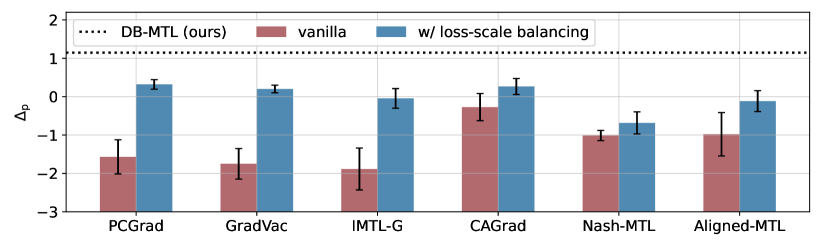
Figure 1: Performance of existing gradient balancing methods with the loss-scale balancing method (i.e., logarithm transformation) on NYUv2. “vanilla” stands for the original method.

Discussion.

Although the logarithm transformation is a simple technique to achieve scale-balancing (Eigen et al., 2014, Girshick, 2015), in MTL, it has only been studied in Navon et al. (2022) as one of the baselines. In this paper, we thoroughly study it and show that integrating it into existing gradient balancing methods (PCGrad (Yu et al., 2020), GradVac (Wang et al., 2021), IMTL-G (Liu et al., 2021b), CAGrad (Liu et al., 2021a), Nash-MTL (Navon et al., 2022), and Aligned-MTL (Senushkin et al., 2023)) improves their performance by a large margin, as shown in Figure 1, demonstrating the effectiveness of balancing loss scales in MTL.

IMTL-L (Liu et al., 2021b) tackles the loss scale issue using a transformed loss $e^{s_{t}}\ell_{t}(\mathcal{D}_{t};{\bm{\theta}},{\bm{\psi}}_{t})-s_{t}$, where $s_{t}$ is a learnable parameter for $t$-th task and approximately solved by one-step gradient descent at every iteration. Hence, it cannot ensure all loss scales are the same in each iteration, while the logarithm transformation can. Proposition A.1 in Appendix shows the logarithm transformation is equivalent to IMTL-L when $s_{t}$ is the exact minimizer in each iteration. Empirically, Figure 3 shows that logarithm transformation consistently outperforms IMTL-L on four datasets (NYUv2, Cityscapes, Office-31, and Office-Home) in terms of $\Delta_{\mathrm{p}}$ (Eq. (3)).

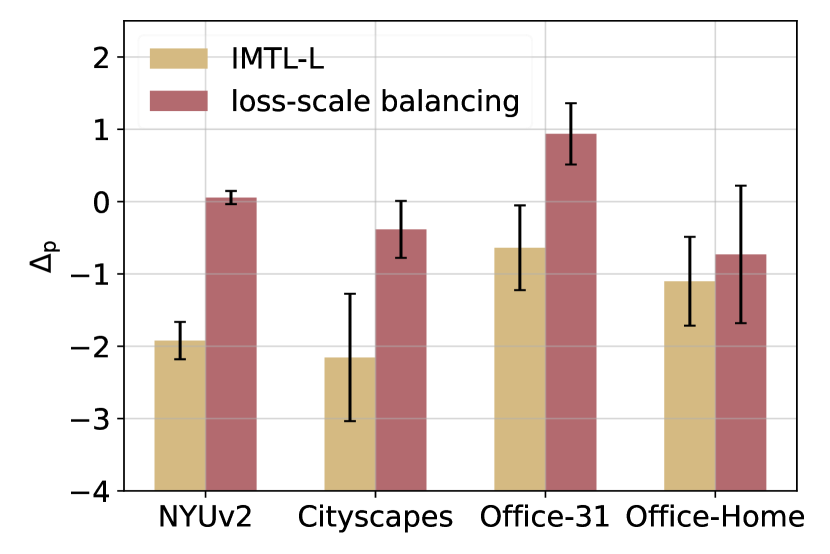
Figure 2: Comparison of IMTL-L (Liu et al., 2021b) and the loss-scale balancing method on four datasets.

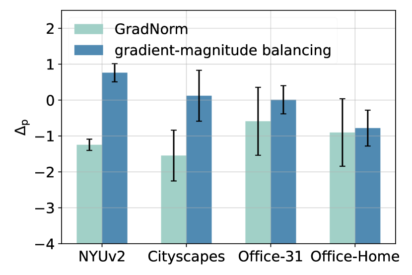
Figure 3: Comparison of GradNorm (Chen et al., 2018b) and the gradient-magnitude balancing method on four datasets.

3.2 Magnitude-Balancing Gradient Normalization

In addition to the scale issue in task losses, task gradients also suffer from the scale issue. The update direction by uniformly averaging all task gradients may be dominated by the large task gradients, causing sub-optimal performance (Yu et al., 2020, Liu et al., 2021a).

A simple approach is to normalize task gradients into the same magnitude. For the task gradients, as computing the batch gradient $\nabla_{{\bm{\theta}}}\log\ell_{t}(\mathcal{D}_{t};{\bm{\theta}},{\bm{\psi}}_{t})$ is computationally expensive, a mini-batch stochastic gradient descent method is always used in practice. Specifically, at iteration $k$, we sample a mini-batch $\mathcal{B}_{t,k}$ from $\mathcal{D}_{t}$ for the $t$-th task ($t=1,\dots,T$) (step 6 in Algorithm 1) and compute the mini-batch gradient ${{\bm{g}}}_{t,k}=\nabla_{{\bm{\theta}}_{k}}\log\ell_{t}(\mathcal{B}_{t,k};{\bm{\theta}}_{k},{\bm{\psi}}_{t,k})$ (step 7 in Algorithm 1). Exponential moving average (EMA), which is popularly used in adaptive gradient methods (e.g., RMSProp (Tieleman & Hinton, 2012), AdaDelta (Zeiler, 2012), and Adam (Kingma & Ba, 2015)), is used to estimate $\mathbb{E}_{\mathcal{B}_{t,k}\sim\mathcal{D}_{t}}\nabla_{{\bm{\theta}}_{k}}\log\ell_{t}(\mathcal{B}_{t,k};{\bm{\theta}}_{k},{\bm{\psi}}_{t,k})$ dynamically (step 8 in Algorithm 1) as

$$\hat{{\bm{g}}}_{t,k}=\beta\hat{{\bm{g}}}_{t,k-1}+(1-\beta){{\bm{g}}}_{t,k},$$

where $\beta\in(0,1)$ controls the forgetting rate. After obtaining the task gradients $\{\hat{{\bm{g}}}_{t,k}\}_{t=1}^{T}$, we normalize them to have the same magnitude $\ell_{2}$ norm, and compute the aggregated gradient as

$$\tilde{{\bm{g}}}_{k}=\alpha_{k}\sum_{t=1}^{T}\frac{\hat{{\bm{g}}}_{t,k}}{\|\hat{{\bm{g}}}_{t,k}\|_{2}},$$ (2)

where $\alpha_{k}$ is a scale factor controlling the update magnitude. After normalization, all tasks contribute equally to the update direction.

The choice of $\alpha_{k}$ is critical for alleviating the task balancing problem. Intuitively, when some tasks have large gradient norms and others have small gradient norms, it means the model ${\bm{\theta}}_{k}$ is close to a point where the former tasks have not yet converged while the latter tasks have converged. Such point is unsatisfactory in MTL and can cause the task balancing problem since we expect all tasks to achieve convergence. Hence, $\alpha_{k}$ should be large enough to escape the unsatisfactory point. When all task gradient norms are small, it indicates the model ${\bm{\theta}}_{k}$ is close to a stationary point of all tasks, $\alpha_{k}$ should be small such that the model will be caught by such point. Thus, we can choose $\alpha_{k}=\max_{1\leq t\leq T}\|\hat{{\bm{g}}}_{t,k}\|_{2}$. Note that $\alpha_{k}$ is small if and only if the norms of all the task gradients are small. Figure 4 shows the performance of using different strategies for adjusting $\alpha_{k}$ on the NYUv2 dataset, where the experimental setup is in Section 4.1. Results on the other datasets are in Appendix (Figure 6). As can be seen, the maximum-norm strategy consistently performs much better, and thus it is used (in step 10 of Algorithm 1).

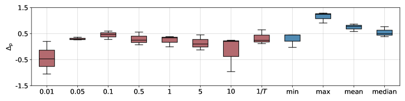
Figure 4: Results of different strategies for $\alpha_{k}$ in Eq. (2) on the NYUv2 dataset in terms of $\Delta_{\mathrm{p}}$. “min”, “max”, “mean”, and “median” denotes the minimum, maximum, average, and median of $\|\hat{{\bm{g}}}_{t,k}\|_{2}~{}(t=1,\dots,T)$, respectively.

After scaling the losses and gradients, the task-sharing parameter is updated as ${\bm{\theta}}_{k+1}={\bm{\theta}}_{k}-\eta\tilde{{\bm{g}}}_{k}$ (step 11), where $\eta>0$ is the learning rate. For the task-specific parameters $\{{\bm{\psi}}_{t,k}\}_{t=1}^{T}$, as the update of each of them only depends on the corresponding task gradient separately, their gradients do not have the gradient scaling issue. Hence, the update for task-specific parameters is ${\bm{\psi}}_{t,k+1}={\bm{\psi}}_{t,k}-\eta\nabla_{{\bm{\psi}}_{t,k}}\log\ell_{t}({\mathcal{B}}_{t,k};{\bm{\theta}}_{k},{\bm{\psi}}_{t,k})$ (steps 12-14).

Algorithm 1 Dual-Balancing Multi-Task Learning.

1:numbers of iterations $K$, learning rate $\eta$, tasks $\{\mathcal{D}_{t}\}_{t=1}^{T}$, $\beta$, $\epsilon=10^{-8}$;

2:randomly initialize ${\bm{\theta}}_{0},\{{\bm{\psi}}_{t,0}\}_{t=1}^{T}$;

3:initialize $\hat{{\bm{g}}}_{t,-1}=\bf{0}$, for all $t$;

4:for $k=0,\dots,K-1$ do

5:     for $t=1,\dots,T$ do

6:         sample a mini-batch dataset $\mathcal{B}_{t,k}$ from $\mathcal{D}_{t}$;

7:         ${\bm{g}}_{t,k}=\nabla_{{\bm{\theta}}_{k}}\log(\ell_{t}({\mathcal{B}}_{t,k};{\bm{\theta}}_{k},{\bm{\psi}}_{t,k})+\epsilon)$;

8:         compute $\hat{{\bm{g}}}_{t,k}=\beta\hat{{\bm{g}}}_{t,k-1}+(1-\beta){\bm{g}}_{t,k}$;

9:     end for

10:     compute $\tilde{{\bm{g}}}_{k}=\alpha_{k}\sum_{t=1}^{T}\frac{\hat{{\bm{g}}}_{t,k}}{\|\hat{{\bm{g}}}_{t,k}\|_{2}+\epsilon}$, where $\alpha_{k}=\max_{1\leq t\leq T}\|\hat{{\bm{g}}}_{t,k}\|_{2}$;

11:     update task-sharing parameter by ${\bm{\theta}}_{k+1}={\bm{\theta}}_{k}-\eta\tilde{{\bm{g}}}_{k}$;

12:     for $t=1,\dots,T$ do

13:         ${\bm{\psi}}_{t,k+1}={\bm{\psi}}_{t,k}-\eta\nabla_{{\bm{\psi}}_{t,k}}\log(\ell_{t}({\mathcal{B}}_{t,k};{\bm{\theta}}_{k},{\bm{\psi}}_{t,k})+\epsilon)$;

14:     end for

15:end for

16:return ${\bm{\theta}}_{K},\{{\bm{\psi}}_{t,K}\}_{t=1}^{T}$.

Discussion. GradNorm (Chen et al., 2018b) aims to learn $\{\gamma_{t}\}_{t=1}^{T}$ so that the scaled gradients have similar norms. However, it has two problems. First, alternating the updates of model parameters and task weights cannot guarantee all task gradients to have the same magnitude in each iteration. Second, from Figures 4 and 6, choice of the update magnitude $\alpha_{k}$ can significantly affect performance, but this is not considered in GradNorm. Figure 3 shows the performance comparison between GradNorm and the proposed gradient-magnitude balancing method on four datasets (NYUv2, Cityscapes, Office-31, and Office-Home). As can be seen, the proposed method achieves better performance than GradNorm in terms of $\Delta_{\mathrm{p}}$ on all datasets.

4 Experiments

In this section, we empirically evaluate the proposed DB-MTL on a number of tasks, including scene understanding (Section 4.1), image classification (Section 4.2), and molecular property prediction (Section 4.3).

4.1 Scene Understanding

Datasets. The following datasets are used: (i) NYUv2(Silberman et al., 2012), which is an indoor scene understanding dataset. It has $3$ tasks ($13$-class semantic segmentation, depth estimation, and surface normal prediction) with $795$ training and $654$ testing images. (ii) Cityscapes(Cordts et al., 2016), which is an urban scene understanding dataset. It has $2$ tasks ($7$-class semantic segmentation and depth estimation) with $2,975$ training and $500$ testing images.

Baselines. The proposed DB-MTL is compared with various types of MTL baselines, including (i) equal weighting (EW) (Zhang & Yang, 2022); (ii) GLS (Chennupati et al., 2019), which minimizes the geometric mean loss $\sqrt[T]{\prod_{t=1}^{T}\ell_{t}(\mathcal{D}_{t};{\bm{\theta}},{\bm{\psi}}_{t})}$; (iii) RLW (Lin et al., 2022), in which the task weights are sampled from the standard normal distribution; (iv) loss balancingmethods including UW (Kendall et al., 2018), DWA (Liu et al., 2019a), and IMTL-L (Liu et al., 2021b); (v) gradient balancingmethods including MGDA (Sener & Koltun, 2018), GradNorm (Chen et al., 2018b), PCGrad (Yu et al., 2020), GradDrop (Chen et al., 2020), GradVac (Wang et al., 2021), IMTL-G (Liu et al., 2021b), CAGrad (Liu et al., 2021a), MTAdam (Malkiel & Wolf, 2021), Nash-MTL (Navon et al., 2022), MetaBalance (He et al., 2022), MoCo (Fernando et al., 2023), and Aligned-MTL (Senushkin et al., 2023); (vi) hybrid balancingmethod that combines loss and gradient balancing: IMTL (Liu et al., 2021b). For comparison, we also include the single-task learning (STL) baseline, which learns each task separately.

All methods are implemented based on the open-source LibMTL library (Lin & Zhang, 2023). For all MTL methods, the hard-parameter sharing (HPS) pattern (Caruana, 1993) is used, which consists of a task-sharing feature encoder and $T$ task-specific heads.

Table 1: Performance on NYUv2 with $3$ tasks. $\uparrow(\downarrow)$ indicates that the higher (lower) the result, the better the performance. The best and second best results are highlighted in bold and underline, respectively.

	Segmentation		Depth Estimation		Surface Normal Prediction					$\Delta_{\mathrm{p}}$${\uparrow}$
	mIoU${\uparrow}$	PAcc$\uparrow$	AErr$\downarrow$	RErr$\downarrow$	Angle Distance		Within $t^{\circ}$
					Mean$\downarrow$	MED$\downarrow$	11.25$\uparrow$	22.5$\uparrow$	30$\uparrow$
STL	$53.50$	$75.39$	$0.3926$	$0.1605$	$\underline{21.99}$	15.16	39.04	65.00	$\underline{75.16}$	$0.00$
EW	$53.93$	$75.53$	$0.3825$	$0.1577$	$23.57$	$17.01$	$35.04$	$60.99$	$72.05$	${\color[rgb]{0.3125,0.54296875,0.69921875}-1.78}_{\pm 0.45}$
GLS	54.59	76.06	$\underline{0.3785}$	0.1555	$22.71$	$16.07$	$36.89$	$63.11$	$73.81$	$\underline{{\color[rgb]{0.703125,0.4140625,0.43359375}+0.30}}_{\pm 0.30}$
RLW	$54.04$	$75.58$	$0.3827$	$0.1588$	$23.07$	$16.49$	$36.12$	$62.08$	$72.94$	${\color[rgb]{0.3125,0.54296875,0.69921875}-1.10}_{\pm 0.40}$
UW	$\underline{54.29}$	$75.64$	$0.3815$	$0.1583$	$23.48$	$16.92$	$35.26$	$61.17$	$72.21$	${\color[rgb]{0.3125,0.54296875,0.69921875}-1.52}_{\pm 0.39}$
DWA	$54.06$	$75.64$	$0.3820$	$0.1564$	$23.70$	$17.11$	$34.90$	$60.74$	$71.81$	${\color[rgb]{0.3125,0.54296875,0.69921875}-1.71}_{\pm 0.25}$
IMTL-L	$53.89$	$75.54$	$0.3834$	$0.1591$	$23.54$	$16.98$	$35.09$	$61.06$	$72.12$	${\color[rgb]{0.3125,0.54296875,0.69921875}-1.92}_{\pm 0.25}$
MGDA	$53.52$	$74.76$	$0.3852$	$0.1566$	$22.74$	$16.00$	$37.12$	$63.22$	$73.84$	${\color[rgb]{0.3125,0.54296875,0.69921875}-0.64}_{\pm 0.25}$
GradNorm	$53.91$	$75.38$	$0.3842$	$0.1571$	$23.17$	$16.62$	$35.80$	$61.90$	$72.84$	${\color[rgb]{0.3125,0.54296875,0.69921875}-1.24}_{\pm 0.15}$
PCGrad	$53.94$	$75.62$	$0.3804$	$0.1578$	$23.52$	$16.93$	$35.19$	$61.17$	$72.19$	${\color[rgb]{0.3125,0.54296875,0.69921875}-1.57}_{\pm 0.44}$
GradDrop	$53.73$	$75.54$	$0.3837$	$0.1580$	$23.54$	$16.96$	$35.17$	$61.06$	$72.07$	${\color[rgb]{0.3125,0.54296875,0.69921875}-1.85}_{\pm 0.39}$
GradVac	$54.21$	$\underline{75.67}$	$0.3859$	$0.1583$	$23.58$	$16.91$	$35.34$	$61.15$	$72.10$	${\color[rgb]{0.3125,0.54296875,0.69921875}-1.75}_{\pm 0.39}$
IMTL-G	$53.01$	$75.04$	$0.3888$	$0.1603$	$23.08$	$16.43$	$36.24$	$62.23$	$73.06$	${\color[rgb]{0.3125,0.54296875,0.69921875}-1.89}_{\pm 0.54}$
CAGrad	$53.97$	$75.54$	$0.3885$	$0.1588$	$22.47$	$15.71$	$37.77$	$63.82$	$74.30$	${\color[rgb]{0.3125,0.54296875,0.69921875}-0.27}_{\pm 0.35}$
MTAdam	$52.67$	$74.86$	$0.3873$	$0.1583$	$23.26$	$16.55$	$36.00$	$61.92$	$72.74$	${\color[rgb]{0.3125,0.54296875,0.69921875}-1.97}_{\pm 0.23}$
Nash-MTL	$53.41$	$74.95$	$0.3867$	$0.1612$	$22.57$	$15.94$	$37.30$	$63.40$	$74.09$	${\color[rgb]{0.3125,0.54296875,0.69921875}-1.01}_{\pm 0.13}$
MetaBalance	$53.92$	$75.57$	$0.3901$	$0.1594$	$22.85$	$16.16$	$36.72$	$62.91$	$73.62$	${\color[rgb]{0.3125,0.54296875,0.69921875}-1.06}_{\pm 0.17}$
MoCo	$52.25$	$74.56$	$0.3920$	$0.1622$	$22.82$	$16.24$	$36.58$	$62.72$	$73.49$	${\color[rgb]{0.3125,0.54296875,0.69921875}-2.25}_{\pm 0.51}$
Aligned-MTL	$52.94$	$75.00$	$0.3884$	$0.1570$	$22.65$	$16.07$	$36.88$	$63.18$	$73.94$	${\color[rgb]{0.3125,0.54296875,0.69921875}-0.98}_{\pm 0.56}$
IMTL	$53.63$	$75.44$	$0.3868$	$0.1592$	$22.58$	$15.85$	$37.44$	$63.52$	$74.09$	${\color[rgb]{0.3125,0.54296875,0.69921875}-0.57}_{\pm 0.24}$
DB-MTL (ours)	$53.92$	$75.60$	0.3768	$\underline{0.1557}$	21.97	$\underline{15.37}$	$\underline{38.43}$	${64.81}$	75.24	${\color[rgb]{0.703125,0.4140625,0.43359375}\textbf{+1.15}}_{\pm 0.16}$

Performance Evaluation. Following Lin et al. (2022), Liu et al. (2019a), we use (i) the mean intersection over union (mIoU) and class-wise pixel accuracy (PAcc) for semantic segmentation; (ii) relative error (RErr) and absolute error (AErr) for depth estimation; (iii) mean and median angle errors, and percentage of normals within $t^{\circ}~{}(t=11.25,22.5,30)$ for surface normal prediction.

Following Maninis et al. (2019), Vandenhende et al. (2021), Lin et al. (2022), we report the relative performance improvement of an MTL method $\mathcal{A}$ over STL, averaged over all the metrics above, i.e.,

$$\Delta_{\mathrm{p}}(\mathcal{A})=\frac{1}{T}\sum_{t=1}^{T}\Delta_{\mathrm{p},t}(\mathcal{A}),\quad\mathrm{where}~{}~{}\Delta_{\mathrm{p},t}(\mathcal{A})=100\%\times\frac{1}{N_{t}}\sum_{i=1}^{N_{t}}(-1)^{s_{t,i}}\frac{M_{t,i}^{\mathcal{A}}-M_{t,i}^{\text{STL}}}{M_{t,i}^{\text{STL}}}.$$ (3)

where $T$ is the number of tasks, $N_{t}$ is the number of metrics for task $t$, $M_{t,i}^{\mathcal{A}}$ is the $i$th metric value of method $\mathcal{A}$ on task $t$, and $s_{t,i}$ is $0$ if a larger value indicates better performance for the $i$th metric on task $t$, and 1 otherwise. Each experiment is repeated three times. Further implementation details can be found in Appendix B.

Results. Table 1 shows the results on NYUv2. As can be seen, the proposed DB-MTL performs the best in terms of $\Delta_{\mathrm{p}}$. Note that most of MTL baselines perform better than STL on semantic segmentation and depth estimation tasks but has a large drop on surface normal prediction task, due to the task balancing problem. Only the proposed DB-MTL has comparable performance with STL on surface normal prediction task and maintains the superiority on the other tasks, which demonstrates its effectiveness.

Table 2 shows the results on Cityscapes. As can be seen, DB-MTL again achieves the best in terms of $\Delta_{\mathrm{p}}$. Note that all MTL baselines perform worse than STL in terms of $\Delta_{\mathrm{p}}$ and only the proposed DB-MTL outperforms STL on all tasks.

Table 2: Performance on Cityscapes with $2$ tasks. $\uparrow(\downarrow)$ indicates that the higher (lower) the result, the better the performance. The best and second best results are highlighted in bold and underline, respectively.

	Segmentation		Depth Estimation		$\Delta_{\mathrm{p}}$${\uparrow}$
	mIoU${\uparrow}$	PAcc$\uparrow$	AErr$\downarrow$	RErr$\downarrow$
STL	$69.06$	$91.54$	$0.01282$	$\underline{43.53}$	$\underline{0.00}$
EW	$68.93$	$91.58$	$0.01315$	$45.90$	${\color[rgb]{0.3125,0.54296875,0.69921875}-2.05}_{\pm 0.56}$
GLS	$68.69$	$91.45$	$0.01280$	$44.13$	${\color[rgb]{0.3125,0.54296875,0.69921875}-0.39}_{\pm 1.06}$
RLW	$69.03$	$91.57$	$0.01343$	$44.77$	${\color[rgb]{0.3125,0.54296875,0.69921875}-1.91}_{\pm 0.21}$
UW	$69.03$	$\underline{91.61}$	$0.01338$	$45.89$	${\color[rgb]{0.3125,0.54296875,0.69921875}-2.45}_{\pm 0.68}$
DWA	$68.97$	$91.58$	$0.01350$	$45.10$	${\color[rgb]{0.3125,0.54296875,0.69921875}-2.24}_{\pm 0.28}$
IMTL-L	$68.98$	$91.59$	$0.01340$	$45.32$	${\color[rgb]{0.3125,0.54296875,0.69921875}-2.15}_{\pm 0.88}$
MGDA	$69.05$	$91.53$	${0.01280}$	$44.07$	${\color[rgb]{0.3125,0.54296875,0.69921875}-0.19}_{\pm 0.30}$
GradNorm	$68.97$	$91.60$	$0.01320$	$44.88$	${\color[rgb]{0.3125,0.54296875,0.69921875}-1.55}_{\pm 0.70}$
PCGrad	$68.95$	$91.58$	$0.01342$	$45.54$	${\color[rgb]{0.3125,0.54296875,0.69921875}-2.36}_{\pm 1.17}$
GradDrop	$68.85$	$91.54$	$0.01354$	$44.49$	${\color[rgb]{0.3125,0.54296875,0.69921875}-2.02}_{\pm 0.74}$
GradVac	$68.98$	$91.58$	$0.01322$	$46.43$	${\color[rgb]{0.3125,0.54296875,0.69921875}-2.45}_{\pm 0.54}$
IMTL-G	$69.04$	$91.54$	$0.01280$	$44.30$	${\color[rgb]{0.3125,0.54296875,0.69921875}-0.46}_{\pm 0.67}$
CAGrad	$68.95$	$91.60$	$0.01281$	$45.04$	${\color[rgb]{0.3125,0.54296875,0.69921875}-0.87}_{\pm 0.88}$
MTAdam	$68.43$	$91.26$	$0.01340$	$45.62$	${\color[rgb]{0.3125,0.54296875,0.69921875}-2.74}_{\pm 0.20}$
Nash-MTL	$68.88$	$91.52$	0.01265	$45.92$	${\color[rgb]{0.3125,0.54296875,0.69921875}-1.11}_{\pm 0.21}$
MetaBalance	$69.02$	$91.56$	$\underline{0.01270}$	$45.91$	${\color[rgb]{0.3125,0.54296875,0.69921875}-1.18}_{\pm 0.58}$
MoCo	69.62	91.76	$0.01360$	$45.50$	${\color[rgb]{0.3125,0.54296875,0.69921875}-2.40}_{\pm 1.50}$
Aligned-MTL	$69.00$	$91.59$	$0.01270$	$44.54$	${\color[rgb]{0.3125,0.54296875,0.69921875}-0.43}_{\pm 0.44}$
IMTL	$69.07$	$91.55$	${0.01280}$	$44.06$	${\color[rgb]{0.3125,0.54296875,0.69921875}-0.32}_{\pm 0.10}$
DB-MTL (ours)	$\underline{69.17}$	$91.56$	${0.01280}$	43.46	${\color[rgb]{0.703125,0.4140625,0.43359375}\textbf{+0.20}}_{\pm 0.40}$

4.2 Image Classification

Datasets.

The following datasets are used: (i) Office-31(Saenko et al., 2010), which contains $4,110$ images from three domains (tasks): Amazon, DSLR, and Webcam. Each task has 31 classes. (ii) Office-Home(Venkateswara et al., 2017), which contains $15,500$ images from four domains (tasks): artistic images, clipart, product images, and real-world images. Each task has $65$ object categories collected under office and home settings. We use the commonly-used data split as in Lin et al. (2022): $60\%$ for training, $20\%$ for validation, and $20\%$ for testing.

Results. Tables 3 and 4 show the results on Office-31 and Office-Home, respectively, using the same set of baselines as in Section 4.1. The testing accuracy of each task is reported and the average testing accuracy among tasks and $\Delta_{\mathrm{p}}$ in Eq. (3) are used as the overall performance metrics. On Office-31, DB-MTL achieves the top testing accuracy on DSLR and Webcam tasks over all baselines and comparable performance on Amazon task. On Office-Home, the performance of DB-MTL on the Artistic, Product, and Real tasks are top two. On both datasets, DB-MTL achieves the best average testing accuracy and $\Delta_{\mathrm{p}}$, showing its effectiveness and demonstrating balancing both loss scale and gradient magnitude is effective.

Table 3: Classification accuracy (%) on Office-31 with $3$ tasks. $\uparrow$ indicates that the higher the result, the better the performance. The best and second best results are highlighted in bold and underline, respectively. Results of MoCo are from Fernando et al. (2023).

	Amazon	DSLR	Webcam	Avg$\uparrow$	$\Delta_{\mathrm{p}}$$\uparrow$
STL	86.61	$95.63$	$96.85$	$93.03$	0.00
EW	$83.53$	$97.27$	$96.85$	$92.55_{\pm 0.62}$	${\color[rgb]{0.3125,0.54296875,0.69921875}-0.61}_{\pm 0.67}$
GLS	$82.84$	$95.62$	$96.29$	$91.59_{\pm 0.58}$	${\color[rgb]{0.3125,0.54296875,0.69921875}-1.63}_{\pm 0.61}$
RLW	$83.82$	$96.99$	$96.85$	$92.55_{\pm 0.89}$	${\color[rgb]{0.3125,0.54296875,0.69921875}-0.59}_{\pm 0.95}$
UW	$83.82$	$97.27$	$96.67$	$92.58_{\pm 0.84}$	${\color[rgb]{0.3125,0.54296875,0.69921875}-0.56}_{\pm 0.90}$
DWA	$83.87$	$96.99$	$96.48$	$92.45_{\pm 0.56}$	${\color[rgb]{0.3125,0.54296875,0.69921875}-0.70}_{\pm 0.62}$
IMTL-L	$84.04$	$96.99$	$96.48$	$92.50_{\pm 0.52}$	${\color[rgb]{0.3125,0.54296875,0.69921875}-0.63}_{\pm 0.58}$
MGDA	$\underline{85.47}$	$95.90$	$97.03$	$92.80_{\pm 0.14}$	${\color[rgb]{0.3125,0.54296875,0.69921875}-0.27}_{\pm 0.15}$
GradNorm	$83.58$	$97.26$	$96.85$	$92.56_{\pm 0.87}$	${\color[rgb]{0.3125,0.54296875,0.69921875}-0.59}_{\pm 0.94}$
PCGrad	$83.59$	$96.99$	$96.85$	$92.48_{\pm 0.53}$	${\color[rgb]{0.3125,0.54296875,0.69921875}-0.68}_{\pm 0.57}$
GradDrop	$84.33$	$96.99$	$96.30$	$92.54_{\pm 0.42}$	${\color[rgb]{0.3125,0.54296875,0.69921875}-0.59}_{\pm 0.46}$
GradVac	$83.76$	$97.27$	$96.67$	$92.57_{\pm 0.73}$	${\color[rgb]{0.3125,0.54296875,0.69921875}-0.58}_{\pm 0.78}$
IMTL-G	$83.41$	$96.72$	$96.48$	$92.20_{\pm 0.89}$	${\color[rgb]{0.3125,0.54296875,0.69921875}-0.97}_{\pm 0.95}$
CAGrad	$83.65$	$95.63$	$96.85$	$92.04_{\pm 0.79}$	${\color[rgb]{0.3125,0.54296875,0.69921875}-1.14}_{\pm 0.85}$
MTAdam	$85.52$	$95.62$	$96.29$	$92.48_{\pm 0.87}$	${\color[rgb]{0.3125,0.54296875,0.69921875}-0.60}_{\pm 0.93}$
Nash-MTL	$85.01$	$\underline{97.54}$	$97.41$	$93.32_{\pm 0.82}$	${\color[rgb]{0.703125,0.4140625,0.43359375}+0.24}_{\pm 0.89}$
MetaBalance	$84.21$	$95.90$	$97.40$	$92.50_{\pm 0.28}$	${\color[rgb]{0.3125,0.54296875,0.69921875}-0.63}_{\pm 0.30}$
MoCo	$84.33$	$\underline{97.54}$	$\underline{98.33}$	$\underline{93.39}$	-
Aligned-MTL	$83.36$	$96.45$	$97.04$	$92.28_{\pm 0.46}$	${\color[rgb]{0.3125,0.54296875,0.69921875}-0.90}_{\pm 0.48}$
IMTL	$83.70$	$96.44$	$96.29$	$92.14_{\pm 0.85}$	${\color[rgb]{0.3125,0.54296875,0.69921875}-1.02}_{\pm 0.92}$
DB-MTL (ours)	$85.12$	98.63	98.51	$\textbf{94.09}_{\pm 0.19}$	${\color[rgb]{0.703125,0.4140625,0.43359375}\textbf{+1.05}}_{\pm 0.20}$

Table 4: Classification accuracy (%) on Office-Home with $4$ tasks. $\uparrow$ indicates that the higher the result, the better the performance. The best and second best results are highlighted in bold and underline, respectively. Results of MoCo are from Fernando et al. (2023).

	Artistic	Clipart	Product	Real	Avg$\uparrow$	$\Delta_{\mathrm{p}}$$\uparrow$
STL	$65.59$	79.60	90.47	$80.00$	$78.91$	$0.00$
EW	$65.34$	$78.04$	$89.80$	$79.50$	$78.17_{\pm 0.37}$	${\color[rgb]{0.3125,0.54296875,0.69921875}-0.92}_{\pm 0.59}$
GLS	$64.51$	$76.85$	$89.83$	$79.56$	$77.69_{\pm 0.27}$	${\color[rgb]{0.3125,0.54296875,0.69921875}-1.58}_{\pm 0.46}$
RLW	$64.96$	$78.19$	$89.48$	80.11	$78.18_{\pm 0.12}$	${\color[rgb]{0.3125,0.54296875,0.69921875}-0.92}_{\pm 0.14}$
UW	$65.97$	$77.65$	$89.41$	$79.28$	$78.08_{\pm 0.30}$	${\color[rgb]{0.3125,0.54296875,0.69921875}-0.98}_{\pm 0.46}$
DWA	$65.27$	$77.64$	$89.05$	$79.56$	$77.88_{\pm 0.28}$	${\color[rgb]{0.3125,0.54296875,0.69921875}-1.26}_{\pm 0.49}$
IMTL-L	$65.90$	$77.28$	$89.37$	$79.38$	$77.98_{\pm 0.38}$	${\color[rgb]{0.3125,0.54296875,0.69921875}-1.10}_{\pm 0.61}$
MGDA	$64.19$	$77.60$	$89.58$	$79.31$	$77.67_{\pm 0.20}$	${\color[rgb]{0.3125,0.54296875,0.69921875}-1.61}_{\pm 0.34}$
GradNorm	$66.28$	$77.86$	$88.66$	$79.60$	$78.10_{\pm 0.63}$	${\color[rgb]{0.3125,0.54296875,0.69921875}-0.90}_{\pm 0.93}$
PCGrad	$\underline{66.35}$	$77.18$	$88.95$	$79.50$	$77.99_{\pm 0.19}$	${\color[rgb]{0.3125,0.54296875,0.69921875}-1.04}_{\pm 0.32}$
GradDrop	$63.57$	$77.86$	$89.23$	$79.35$	$77.50_{\pm 0.23}$	${\color[rgb]{0.3125,0.54296875,0.69921875}-1.86}_{\pm 0.24}$
GradVac	$65.21$	$77.43$	$89.23$	$78.95$	$77.71_{\pm 0.19}$	${\color[rgb]{0.3125,0.54296875,0.69921875}-1.49}_{\pm 0.28}$
IMTL-G	$64.70$	$77.17$	$89.61$	$79.45$	$77.98_{\pm 0.38}$	${\color[rgb]{0.3125,0.54296875,0.69921875}-1.10}_{\pm 0.61}$
CAGrad	$64.01$	$77.50$	$89.65$	$79.53$	$77.73_{\pm 0.16}$	${\color[rgb]{0.3125,0.54296875,0.69921875}-1.50}_{\pm 0.29}$
MTAdam	$62.23$	$77.86$	$88.73$	$77.94$	$76.69_{\pm 0.65}$	${\color[rgb]{0.3125,0.54296875,0.69921875}-2.94}_{\pm 0.85}$
Nash-MTL	$66.29$	$78.76$	$90.04$	80.11	$\underline{78.80}_{\pm 0.52}$	$\underline{{\color[rgb]{0.3125,0.54296875,0.69921875}-0.08}}_{\pm 0.69}$
MetaBalance	$64.01$	$77.50$	$89.72$	$79.24$	$77.61_{\pm 0.42}$	${\color[rgb]{0.3125,0.54296875,0.69921875}-1.70}_{\pm 0.54}$
MoCo	$63.38$	$\underline{79.41}$	$90.25$	$78.70$	$77.93$	-
Aligned-MTL	$64.33$	$76.96$	$89.87$	$79.93$	$77.77_{\pm 0.70}$	${\color[rgb]{0.3125,0.54296875,0.69921875}-1.50}_{\pm 0.89}$
IMTL	$64.07$	$76.85$	$89.65$	$79.81$	$77.59_{\pm 0.29}$	${\color[rgb]{0.3125,0.54296875,0.69921875}-1.72}_{\pm 0.45}$
DB-MTL (ours)	67.42	$77.89$	$\underline{90.43}$	$\underline{80.07}$	$\textbf{78.95}_{\pm 0.35}$	${\color[rgb]{0.703125,0.4140625,0.43359375}\textbf{+0.17}}_{\pm 0.44}$

4.3 Molecular Property Prediction

Dataset. The following dataset is used: QM9 (Ramakrishnan et al., 2014), which is a molecular property prediction dataset with $11$ tasks. Each task performs regression on one property. We use the commonly-used split as in Fey & Lenssen (2019), Navon et al. (2022): $110,000$ for training, $10,000$ for validation, and $10,000$ for testing. Following Fey & Lenssen (2019), Navon et al. (2022), we use the mean absolute error (MAE) for performance evaluation on each task.

Results. Table 5 shows each task’s testing MAE and overall performance $\Delta_{\mathrm{p}}$ (Eq. (3)) on QM9, using the same set of baselines as in Section 4.1. Note that QM9 is a challenging dataset in MTL and none of the MTL methods performs better than STL, as observed in previous works (Gasteiger et al., 2020, Navon et al., 2022). DB-MTL performs the best among all MTL methods and greatly improves over the second-best MTL method, Nash-MTL, in terms of $\Delta_{\mathrm{p}}$.

Table 5: Performance on QM9 with $11$ tasks. $\uparrow(\downarrow)$ indicates that the higher (lower) the result, the better the performance. The best and second best results are highlighted in bold and underline, respectively.

	$\bm{\mu}$	$\bm{\alpha}$	$\bm{\epsilon_{\mathrm{HOMO}}}$	$\bm{\epsilon_{\mathrm{LUMO}}}$	$\bm{\langle R^{2}\rangle}$	ZPVE	$\bm{U_{0}}$	$\bm{U}$	$\bm{H}$	$\bm{G}$	$\bm{c_{v}}$	$\Delta_{\mathrm{p}}$${\uparrow}$
STL	0.062	0.192	58.82	51.95	0.529	$4.52$	$63.69$	$60.83$	$68.33$	$60.31$	0.069	0.00
EW	${0.096}$	$0.286$	$67.46$	${82.80}$	$4.655$	$12.4$	$128.3$	$128.8$	$129.2$	$125.6$	$0.116$	${\color[rgb]{0.3125,0.54296875,0.69921875}-146.3}_{\pm 7.86}$
GLS	$0.332$	$0.340$	$143.1$	$131.5$	$1.023$	4.45	53.35	53.79	53.78	53.34	$0.111$	${\color[rgb]{0.3125,0.54296875,0.69921875}-81.16}_{\pm 15.5}$
RLW	$0.112$	$0.331$	$74.59$	$90.48$	$6.015$	$15.6$	$156.0$	$156.8$	$157.3$	$151.6$	$0.133$	${\color[rgb]{0.3125,0.54296875,0.69921875}-200.9}_{\pm 13.4}$
UW	$0.336$	$0.382$	$155.1$	$144.3$	$0.965$	$4.58$	$61.41$	$61.79$	$61.83$	$61.40$	$0.116$	${\color[rgb]{0.3125,0.54296875,0.69921875}-92.35}_{\pm 13.9}$
DWA	$0.103$	$0.311$	$71.55$	$87.21$	$4.954$	$13.1$	$134.9$	$135.8$	$136.3$	$132.0$	$0.121$	${\color[rgb]{0.3125,0.54296875,0.69921875}-160.9}_{\pm 16.7}$
IMTL-L	$0.277$	$0.355$	$150.1$	$135.2$	$\underline{0.946}$	$\underline{4.46}$	$\underline{58.08}$	$\underline{58.43}$	$\underline{58.46}$	$\underline{58.06}$	$0.110$	${\color[rgb]{0.3125,0.54296875,0.69921875}-77.06}_{\pm 11.1}$
MGDA	$0.181$	$0.325$	$118.6$	$92.45$	$2.411$	$5.55$	$103.7$	$104.2$	$104.4$	$103.7$	$0.110$	${\color[rgb]{0.3125,0.54296875,0.69921875}-103.0}_{\pm 8.62}$
GradNorm	$0.114$	$0.341$	$\underline{67.17}$	$84.66$	$7.079$	$14.6$	$173.2$	$173.8$	$174.4$	$168.9$	$0.147$	${\color[rgb]{0.3125,0.54296875,0.69921875}-227.5}_{\pm 1.85}$
PCGrad	$0.104$	$0.293$	$75.29$	$88.99$	$3.695$	$8.67$	$115.6$	$116.0$	$116.2$	$113.8$	$0.109$	${\color[rgb]{0.3125,0.54296875,0.69921875}-117.8}_{\pm 3.97}$
GradDrop	$0.114$	$0.349$	$75.94$	$94.62$	$5.315$	$15.8$	$155.2$	$156.1$	$156.6$	$151.9$	$0.136$	${\color[rgb]{0.3125,0.54296875,0.69921875}-191.4}_{\pm 9.62}$
GradVac	$0.100$	$0.299$	$68.94$	$84.14$	$4.833$	$12.5$	$127.3$	$127.8$	$128.1$	$124.7$	$0.117$	${\color[rgb]{0.3125,0.54296875,0.69921875}-150.7}_{\pm 7.41}$
IMTL-G	$0.670$	$0.978$	$220.7$	$249.7$	$19.48$	$55.6$	$1109$	$1117$	$1123$	$1043$	$0.392$	${\color[rgb]{0.3125,0.54296875,0.69921875}-1250}_{\pm 90.9}$
CAGrad	$0.107$	$0.296$	$75.43$	$88.59$	$2.944$	$6.12$	$93.09$	$93.68$	$93.85$	$92.32$	$0.106$	${\color[rgb]{0.3125,0.54296875,0.69921875}-87.25}_{\pm 1.51}$
MTAdam	$0.593$	$1.352$	$232.3$	$419.0$	$24.31$	$69.7$	$1060$	$1067$	$1070$	$1007$	$0.627$	${\color[rgb]{0.3125,0.54296875,0.69921875}-1403}_{\pm 203}$
Nash-MTL	$0.115$	$\underline{0.263}$	$85.54$	$86.62$	$2.549$	$5.85$	$83.49$	$83.88$	$84.05$	$82.96$	$\underline{0.097}$	${\color[rgb]{0.3125,0.54296875,0.69921875}-73.92}_{\pm 2.12}$
MetaBalance	$\underline{0.090}$	$0.277$	$70.50$	$\underline{78.43}$	$4.192$	$11.2$	$113.7$	$114.2$	$114.5$	$111.7$	$0.110$	${\color[rgb]{0.3125,0.54296875,0.69921875}-125.1}_{\pm 7.98}$
MoCo	$0.489$	$1.096$	$189.5$	$247.3$	$34.33$	$64.5$	$754.6$	$760.1$	$761.6$	$720.3$	$0.522$	${\color[rgb]{0.3125,0.54296875,0.69921875}-1314}_{\pm 65.2}$
Aligned-MTL	$0.123$	$0.295$	$98.07$	$94.56$	$2.397$	$5.90$	$86.42$	$87.42$	$87.19$	$86.75$	$0.106$	${\color[rgb]{0.3125,0.54296875,0.69921875}-80.58}_{\pm 4.18}$
IMTL	$0.138$	$0.344$	$106.1$	$102.9$	$2.595$	$7.84$	$102.5$	$103.0$	$103.2$	$100.8$	$0.110$	${\color[rgb]{0.3125,0.54296875,0.69921875}-104.3}_{\pm 11.7}$
DB-MTL (ours)	$0.112$	$0.264$	$89.26$	$86.59$	$2.429$	$5.41$	$60.33$	$60.78$	$60.80$	$60.59$	$0.098$	$\underline{{\color[rgb]{0.3125,0.54296875,0.69921875}-58.10}}_{\pm 3.89}$

4.4 Ablation Study

DB-MTL has two components: the loss-scale balancing method (i.e., logarithm transformation) in Section 3.1 and the gradient-magnitude balancing method in Section 3.2. In this experiment, we study the effectiveness of each component. We consider the four combinations: (i) use neither loss-scale nor gradient-magnitude balancing methods (i.e., the EW baseline); (ii) use only loss-scale balancing; (iii) use only gradient-magnitude balancing; (iv) use both loss-scale and gradient-magnitude balancing methods (i.e., the proposed DB-MTL). Table 6 shows the $\Delta_{\mathrm{p}}$ of different combinations on five datasets, i.e., NYUv2, Cityscapes, Office-31, Office-Home, and QM9. As can be seen, on all datasets, both components are beneficial to DB-MTL and combining them achieves the best performance.

Table 6: Ablation study of DB-MTL on different datasets in terms of $\Delta_{\mathrm{p}}$.

loss-scale	gradient-magnitude	NYUv2	Cityscapes	Office-31	Office-Home	QM9
balancing	balancing
✗	✗	${-1.78}_{\pm 0.45}$	${-2.05}_{\pm 0.56}$	${-0.61}_{\pm 0.67}$	${-0.92}_{\pm 0.59}$	${-146.3}_{\pm 7.86}$
✓	✗	$+0.06_{\pm 0.09}$	$-0.38_{\pm 0.39}$	$+0.93_{\pm 0.42}$	$-0.73_{\pm 0.95}$	$-74.40_{\pm 13.2}$
✗	✓	$+0.76_{\pm 0.25}$	$+0.12_{\pm 0.70}$	$+0.01_{\pm 0.39}$	$-0.78_{\pm 0.49}$	$-65.73_{\pm 2.86}$
✓	✓	$\textbf{+1.15}_{\pm 0.16}$	$\textbf{+0.20}_{\pm 0.40}$	$\textbf{+1.05}_{\pm 0.20}$	$\textbf{+0.17}_{\pm 0.44}$	$\textbf{-58.10}_{\pm 3.89}$

5 Conclusion

In this paper, we alleviate the task-balancing problem in MTL by presenting Dual-Balancing Multi-Task Learning (DB-MTL), a novel approach that consists of loss-scale and gradient-magnitude balancing methods. The former ensures all task losses have the same scale via the logarithm transformation, while the latter guarantees that all task gradients have the same magnitude as the maximum gradient norm by a gradient normalization. Extensive experiments on a number of benchmark datasets demonstrate that DB-MTL achieves state-of-the-art performance.

Appendix

Appendix A Analysis

Proposition A.1.

For $x>0$, $\log(x)=\min_{s}e^{s}x-s-1$.

Proof.

Define an auxiliary function $f(s)=e^{s}x-s-1$. It is easy to show that $\derivative{f(s)}{s}=e^{s}x-1$ and $\derivative[2]{f(s)}{s}=e^{s}x>0$. Thus, $f(s)$ is convex. By the first-order optimal condition (Boyd & Vandenberghe, 2004), let $e^{s^{\star}}x-1=0$, the global minimizer is solved as $s^{\star}=-\log(x)$. Therefore, $f(s^{\star})=e^{s^{\star}}x-s^{\star}-1=e^{-\log(x)}x+\log(x)-1=\log(x)$, where we finish the proof. ∎

Appendix B Implementation Details for Section 4

NYUv2 and Cityscapes. Following Lin et al. (2022), we use the DeepLabV3+ network (Chen et al., 2018a), containing a ResNet-50 network with dilated convolutions pre-trained on the ImageNet dataset (Deng et al., 2009) as the shared encoder and the Atrous Spatial Pyramid Pooling (Chen et al., 2018a) module as the task-specific head. We train the model for $200$ epochs by using the Adam optimizer (Kingma & Ba, 2015) with learning rate $10^{-4}$ and weight decay $10^{-5}$. The learning rate is halved to $5\times 10^{-5}$ after $100$ epochs. The cross-entropy loss, $L_{1}$ loss, and cosine loss are used as the loss functions of the semantic segmentation, depth estimation, and surface normal prediction tasks, respectively. All input images are resized to $288\times 384$, and the batch size is set to $8$ for training for NYUv2. We resize the input images to $128\times 256$, and use the batch size $64$ for training for Cityscapes.

Office-31 and Office-Home. Following Lin et al. (2022), a ResNet-18 (He et al., 2016) pre-trained on the ImageNet dataset (Deng et al., 2009) is used as a shared encoder, and a linear layer is used as a task-specific head. We resize the input image to $224\times 224$. The batch size and the training epoch are set to $64$ and $100$, respectively. The Adam optimizer (Kingma & Ba, 2015) with the learning rate as $10^{-4}$ and the weight decay as $10^{-5}$ is used. The cross-entropy loss is used for all the tasks and classification accuracy is used as the evaluation metric.

QM9. Following Fey & Lenssen (2019), Navon et al. (2022), a graph neural network (Gilmer et al., 2017) is used as the shared encoder, and a linear layer is used as the task-specific head. The targets of each task are normalized to have zero mean and unit standard deviation. The batch size and training epoch are set to $128$ and $300$, respectively. The Adam optimizer (Kingma & Ba, 2015) with the learning rate $0.001$ is used for training and the ReduceLROnPlateau scheduler (Paszke et al., 2019) is used to reduce the learning rate once $\Delta_{\mathrm{p}}$ on the validation dataset stops improving. Following Fey & Lenssen (2019), Navon et al. (2022), we use mean squared error (MSE) as the loss function.

Following Fernando et al. (2023), for each dataset, we perform grid search for $\beta$ over $\{0.1,0.5,0.9,\frac{0.1}{k^{0.5}},\frac{0.5}{k^{0.5}},\frac{0.9}{k^{0.5}}\}$, where $k$ is the number of iterations.

Appendix C Additional Experimental Results

C.1 Effects of MTL Architectures

The proposed DB-MTL is agnostic to the choice of MTL architectures. In this section, we evaluate DB-MTL on NYUv2 using two more MTL architectures: Cross-stitch (Misra et al., 2016) and MTAN (Liu et al., 2019a). Two current state-of-the-art GLS and CAGrad are compared with. The implementation details are the same as those in HPS architecture in Appendix B. Figure 5 shows each task’s improvement performance $\Delta_{\mathrm{p},t}$. For Cross-stitch (Figure 5(a)), as can be seen, DB-MTL performs the best on all tasks, showing its effectiveness. As for MTAN (Figure 5(b)), compared with STL, the MTL methods (GLS, CAGrad, and DB-MTL) perform better on both semantic segmentation and depth estimation tasks, but only DB-MTL achieves comparable performance on the surface normal prediction task.

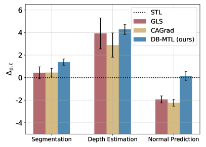
(a) Cross-stitch.

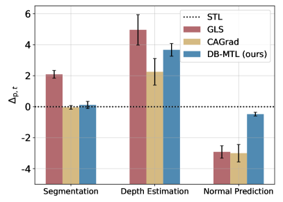
(b) MTAN.

Figure 5: Performance on NYUv2 for Cross-stitch and MTAN architectures.

Furthermore, we conduct experiments to evaluate DB-MTL on NYUv2 with SegNet network (Badrinarayanan et al., 2017). The implementation details are same as those in Appendix B, except that the batch size is set to $2$ and the data augmentation is used following Liu et al. (2021a). The results are shown in Table 7. As can be seen, DB-MTL again achieves the best performance in terms of $\Delta_{\mathrm{p}}$, demonstrating the effectiveness of the proposed method.

Table 7: Performance on the NYUv2 dataset with SegNet network. $\uparrow(\downarrow)$ indicates that the higher (lower) the result, the better the performance. The best and second best results are highlighted in bold and underline, respectively. Superscripts $\sharp$, $\S$, ${\ddagger}$, and $*$ denote the results are from Liu et al. (2021a), Navon et al. (2022), Fernando et al. (2023), and Senushkin et al. (2023), respectively.

	Segmentation		Depth Estimation		Surface Normal Prediction					$\Delta_{\mathrm{p}}$$\uparrow$
	mIoU${\uparrow}$	PAcc$\uparrow$	AErr$\downarrow$	RErr$\downarrow$	Angle Distance		Within $t^{\circ}$
					Mean$\downarrow$	MED$\downarrow$	11.25$\uparrow$	22.5$\uparrow$	30$\uparrow$
STL§	$38.30$	$63.76$	$0.6754$	$0.2780$	$25.01$	$\underline{19.21}$	$\underline{30.14}$	$\underline{57.20}$	$69.15$	$0.00$
EW§	$39.29$	$65.33$	$0.5493$	$0.2263$	$28.15$	$23.96$	$22.09$	$47.50$	$61.08$	${\color[rgb]{0.703125,0.4140625,0.43359375}+0.88}$
GLS	$39.78$	$65.63$	$0.5318$	$0.2272$	$26.13$	$21.08$	$26.57$	$52.83$	$65.78$	${\color[rgb]{0.703125,0.4140625,0.43359375}+5.15}$
RLW§	$37.17$	$63.77$	$0.5759$	$0.2410$	$28.27$	$24.18$	$22.26$	$47.05$	$60.62$	${\color[rgb]{0.3125,0.54296875,0.69921875}-2.16}$
UW§	$36.87$	$63.17$	$0.5446$	$0.2260$	$27.04$	$22.61$	$23.54$	$49.05$	$63.65$	${\color[rgb]{0.703125,0.4140625,0.43359375}+0.91}$
DWA§	$39.11$	$65.31$	$0.5510$	$0.2285$	$27.61$	$23.18$	$24.17$	$50.18$	$62.39$	${\color[rgb]{0.703125,0.4140625,0.43359375}+1.93}$
IMTL-L	$39.78$	$65.27$	$0.5408$	$0.2347$	$26.26$	$20.99$	$26.42$	$53.03$	$65.94$	${\color[rgb]{0.703125,0.4140625,0.43359375}+4.39}$
MGDA§	$30.47$	$59.90$	$0.6070$	$0.2555$	$\underline{24.88}$	$19.45$	$29.18$	$56.88$	$\underline{69.36}$	${\color[rgb]{0.3125,0.54296875,0.69921875}-1.66}$
GradNorm∗	$20.09$	$52.06$	$0.7200$	$0.2800$	24.83	18.86	30.81	57.94	69.73	${\color[rgb]{0.3125,0.54296875,0.69921875}-11.7}$
PCGrad§	$38.06$	$64.64$	$0.5550$	$0.2325$	$27.41$	$22.80$	$23.86$	$49.83$	$63.14$	${\color[rgb]{0.703125,0.4140625,0.43359375}+1.11}$
GradDrop§	$39.39$	$65.12$	$0.5455$	$0.2279$	$27.48$	$22.96$	$23.38$	$49.44$	$62.87$	${\color[rgb]{0.703125,0.4140625,0.43359375}+2.07}$
GradVac∗	$37.53$	$64.35$	$0.5600$	$0.2400$	$27.66$	$23.38$	$22.83$	$48.66$	$62.21$	${\color[rgb]{0.3125,0.54296875,0.69921875}-0.49}$
IMTL-G§	$39.35$	$65.60$	$0.5426$	$0.2256$	$26.02$	$21.19$	$26.20$	$53.13$	$66.24$	${\color[rgb]{0.703125,0.4140625,0.43359375}+4.77}$
CAGrad♯	$39.18$	$64.97$	$0.5379$	$0.2229$	$25.42$	$20.47$	$27.37$	$54.73$	$67.73$	${\color[rgb]{0.703125,0.4140625,0.43359375}+5.81}$
MTAdam	$39.44$	$65.73$	$0.5326$	$0.2211$	$27.53$	$22.70$	$24.04$	$49.61$	$62.69$	${\color[rgb]{0.703125,0.4140625,0.43359375}+3.21}$
Nash-MTL§	$40.13$	$65.93$	$\underline{0.5261}$	$0.2171$	$25.26$	$20.08$	$28.40$	$55.47$	$68.15$	${\color[rgb]{0.703125,0.4140625,0.43359375}+7.65}$
MetaBalance	$39.85$	$65.13$	$0.5445$	$0.2261$	$27.35$	$22.66$	$23.70$	$49.69$	$63.09$	${\color[rgb]{0.703125,0.4140625,0.43359375}+2.67}$
MoCo‡	$40.30$	$66.07$	$0.5575$	0.2135	$26.67$	$21.83$	$25.61$	$51.78$	$64.85$	${\color[rgb]{0.703125,0.4140625,0.43359375}+4.85}$
Aligned-MTL∗	$40.82$	$66.33$	$0.5300$	$0.2200$	$25.19$	$19.71$	$28.88$	$56.23$	$68.54$	$\underline{{\color[rgb]{0.703125,0.4140625,0.43359375}+8.16}}$
IMTL	$\underline{41.19}$	$\underline{66.37}$	$0.5323$	$0.2237$	$26.06$	$20.77$	$26.76$	$53.48$	$66.32$	${\color[rgb]{0.703125,0.4140625,0.43359375}+6.45}$
DB-MTL (ours)	41.42	66.45	0.5251	$\underline{0.2160}$	$25.03$	$19.50$	$28.72$	$56.17$	$68.73$	+8.91

C.2 Effects of $\alpha_{k}$

Figure 6 shows the results of different strategies of $\alpha_{k}$ on the Cityscapes, Office-31, Office-Home, and QM9 datasets, respectively. As can be seen, the strategy of normalizing to the maximum gradient norm is consistently better.

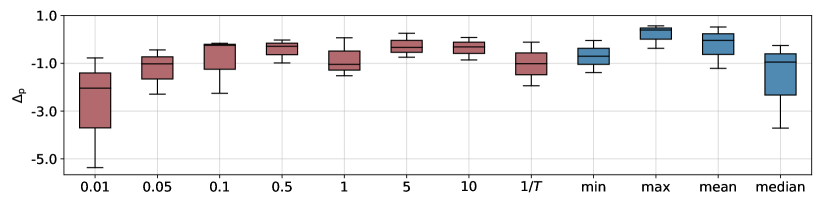
(a) Cityscapes dataset.

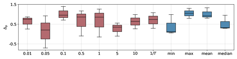
(b) Office-31 dataset.

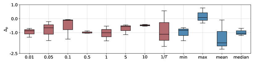
(c) Office-Home dataset.

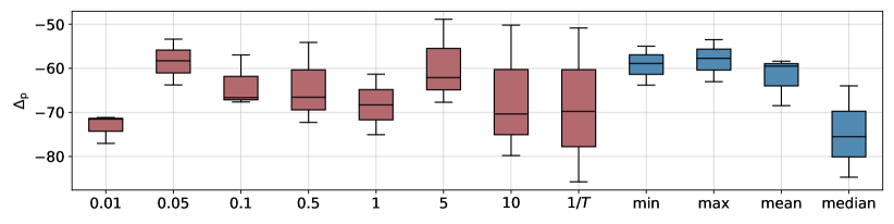
(d) QM9 dataset.

Figure 6: Results of different strategies for $\alpha_{k}$ in Eq. (2) on different datasets in terms of $\Delta_{\mathrm{p}}$. “min”, “max”, “mean”, and “median” denotes the minimum, maximum, average, and median of $\|\hat{{\bm{g}}}_{t,k}\|_{2}~{}(t=1,\dots,T)$, respectively.

C.3 Effects of $\beta$

Table 8 shows the results of DB-MTL with different $\beta$ on Office-31 dataset in terms of the average classification accuracy and $\Delta_{\mathrm{p}}$. As can be seen, DB-MTL is insensitive over a large range of $\beta$ (i.e., $\{0.1/k^{0.5},0.2/k^{0.5},...,0.9/k^{0.5}\}$) and performs better than DB-MTL without EMA ($\beta=0$).

Table 8: Effects of $\beta$ on Office-31 dataset.

$\beta$	Avg$\uparrow$	$\Delta_{\mathrm{p}}$$\uparrow$
$0$	$93.89_{\pm 0.09}$	$+0.84_{\pm 0.09}$
$0.1/k^{0.5}$	${94.09}_{\pm 0.19}$	$+1.05_{\pm 0.20}$
$0.2/k^{0.5}$	$94.02_{\pm 0.42}$	$+0.97_{\pm 0.47}$
$0.3/k^{0.5}$	$94.15_{\pm 0.51}$	$+1.12_{\pm 0.55}$
$0.4/k^{0.5}$	$94.20_{\pm 0.22}$	$+1.18_{\pm 0.23}$
$0.5/k^{0.5}$	$94.01_{\pm 0.56}$	$+0.97_{\pm 0.60}$
$0.6/k^{0.5}$	$94.05_{\pm 0.56}$	$+1.01_{\pm 0.61}$
$0.7/k^{0.5}$	$94.01_{\pm 0.26}$	$+0.96_{\pm 0.30}$
$0.8/k^{0.5}$	$94.00_{\pm 0.16}$	$+0.94_{\pm 0.19}$
$0.9/k^{0.5}$	$94.09_{\pm 0.08}$	$+1.07_{\pm 0.08}$
$0.1$	$93.79_{\pm 0.29}$	$+0.73_{\pm 0.29}$
$0.2$	$93.15_{\pm 0.61}$	$+0.06_{\pm 0.67}$
$0.3$	$92.91_{\pm 0.41}$	$-0.23_{\pm 0.45}$
$0.4$	$93.08_{\pm 0.68}$	$-0.01_{\pm 0.70}$
$0.5$	$92.47_{\pm 0.69}$	$-0.68_{\pm 0.74}$
$0.6$	$92.41_{\pm 0.31}$	$-0.76_{\pm 0.35}$
$0.7$	$92.52_{\pm 0.36}$	$-0.69_{\pm 0.36}$
$0.8$	$92.29_{\pm 0.28}$	$-0.94_{\pm 0.34}$
$0.9$	$90.67_{\pm 0.56}$	$-2.74_{\pm 0.66}$

References

• Badrinarayanan et al. (2017) Vijay Badrinarayanan, Alex Kendall, and Roberto Cipolla. SegNet: A deep convolutional encoder-decoder architecture for image segmentation. IEEE Transactions on Pattern Analysis and Machine Intelligence, 39(12):2481–2495, 2017.
• Boyd & Vandenberghe (2004) Stephen Boyd and Lieven Vandenberghe. Convex optimization. Cambridge University Press, 2004.
• Caruana (1993) Rich Caruana. Multitask learning: A knowledge-based source of inductive bias. In International Conference on Machine Learning, 1993.
• Caruana (1997) Rich Caruana. Multitask learning. Machine Learning, 28(1):41–75, 1997.
• Chen et al. (2018a) Liang-Chieh Chen, Yukun Zhu, George Papandreou, Florian Schroff, and Hartwig Adam. Encoder-decoder with atrous separable convolution for semantic image segmentation. In European Conference on Computer Vision, 2018a.
• Chen et al. (2021) Shijie Chen, Yu Zhang, and Qiang Yang. Multi-task learning in natural language processing: An overview. Preprint arXiv:2109.09138, 2021.
• Chen et al. (2018b) Zhao Chen, Vijay Badrinarayanan, Chen-Yu Lee, and Andrew Rabinovich. GradNorm: Gradient normalization for adaptive loss balancing in deep multitask networks. In International Conference on Machine Learning, 2018b.
• Chen et al. (2020) Zhao Chen, Jiquan Ngiam, Yanping Huang, Thang Luong, Henrik Kretzschmar, Yuning Chai, and Dragomir Anguelov. Just pick a sign: Optimizing deep multitask models with gradient sign dropout. In Neural Information Processing Systems, 2020.
• Chennupati et al. (2019) Sumanth Chennupati, Ganesh Sistu, Senthil Yogamani, and Samir A Rawashdeh. MultiNet++: Multi-stream feature aggregation and geometric loss strategy for multi-task learning. In IEEE Conference on Computer Vision and Pattern Recognition Workshops, 2019.
• Cordts et al. (2016) Marius Cordts, Mohamed Omran, Sebastian Ramos, Timo Rehfeld, Markus Enzweiler, Rodrigo Benenson, Uwe Franke, Stefan Roth, and Bernt Schiele. The cityscapes dataset for semantic urban scene understanding. In IEEE Conference on Computer Vision and Pattern Recognition, 2016.
• Deng et al. (2009) Jia Deng, Wei Dong, Richard Socher, Li-Jia Li, Kai Li, and Li Fei-Fei. ImageNet: A large-scale hierarchical image database. In IEEE Conference on Computer Vision and Pattern Recognition, 2009.
• Désidéri (2012) Jean-Antoine Désidéri. Multiple-gradient descent algorithm (MGDA) for multiobjective optimization. Comptes Rendus Mathematique, 350(5):313–318, 2012.
• Eigen et al. (2014) David Eigen, Christian Puhrsch, and Rob Fergus. Depth map prediction from a single image using a multi-scale deep network. In Neural Information Processing Systems, 2014.
• Fernando et al. (2023) Heshan Devaka Fernando, Han Shen, Miao Liu, Subhajit Chaudhury, Keerthiram Murugesan, and Tianyi Chen. Mitigating gradient bias in multi-objective learning: A provably convergent approach. In International Conference on Learning Representations, 2023.
• Fey & Lenssen (2019) Matthias Fey and Jan Eric Lenssen. Fast graph representation learning with pytorch geometric. Preprint arXiv:1903.02428, 2019.
• Gasteiger et al. (2020) Johannes Gasteiger, Janek Groß, and Stephan Günnemann. Directional message passing for molecular graphs. In International Conference on Learning Representations, 2020.
• Gilmer et al. (2017) Justin Gilmer, Samuel S Schoenholz, Patrick F Riley, Oriol Vinyals, and George E Dahl. Neural message passing for quantum chemistry. In International Conference on Machine Learning, 2017.
• Girshick (2015) Ross Girshick. Fast R-CNN. In IEEE International Conference on Computer Vision, 2015.
• Hazimeh et al. (2021) Hussein Hazimeh, Zhe Zhao, Aakanksha Chowdhery, Maheswaran Sathiamoorthy, Yihua Chen, Rahul Mazumder, Lichan Hong, and Ed Chi. Dselect-k: Differentiable selection in the mixture of experts with applications to multi-task learning. In Neural Information Processing Systems, 2021.
• He et al. (2016) Kaiming He, Xiangyu Zhang, Shaoqing Ren, and Jian Sun. Deep residual learning for image recognition. In IEEE Conference on Computer Vision and Pattern Recognition, 2016.
• He et al. (2022) Yun He, Xue Feng, Cheng Cheng, Geng Ji, Yunsong Guo, and James Caverlee. MetaBalance: improving multi-task recommendations via adapting gradient magnitudes of auxiliary tasks. In ACM Web Conference, 2022.
• Kendall et al. (2018) Alex Kendall, Yarin Gal, and Roberto Cipolla. Multi-task learning using uncertainty to weigh losses for scene geometry and semantics. In IEEE Conference on Computer Vision and Pattern Recognition, 2018.
• Kingma & Ba (2015) Diederik P Kingma and Jimmy Ba. Adam: A method for stochastic optimization. In International Conference on Learning Representations, 2015.
• Kurin et al. (2022) Vitaly Kurin, Alessandro De Palma, Ilya Kostrikov, Shimon Whiteson, and M Pawan Kumar. In defense of the unitary scalarization for deep multi-task learning. In Neural Information Processing Systems, 2022.
• Lin & Zhang (2023) Baijiong Lin and Yu Zhang. LibMTL: A Python library for multi-task learning. Journal of Machine Learning Research, 24(209):1–7, 2023.
• Lin et al. (2022) Baijiong Lin, Feiyang Ye, Yu Zhang, and Ivor Tsang. Reasonable effectiveness of random weighting: A litmus test for multi-task learning. Transactions on Machine Learning Research, 2022.
• Liu et al. (2021a) Bo Liu, Xingchao Liu, Xiaojie Jin, Peter Stone, and Qiang Liu. Conflict-averse gradient descent for multi-task learning. In Neural Information Processing Systems, 2021a.
• Liu et al. (2021b) Liyang Liu, Yi Li, Zhanghui Kuang, Jing-Hao Xue, Yimin Chen, Wenming Yang, Qingmin Liao, and Wayne Zhang. Towards impartial multi-task learning. In International Conference on Learning Representations, 2021b.
• Liu et al. (2017) Pengfei Liu, Xipeng Qiu, and Xuan-Jing Huang. Adversarial multi-task learning for text classification. In Annual Meeting of the Association for Computational Linguistics, 2017.
• Liu et al. (2019a) Shikun Liu, Edward Johns, and Andrew J. Davison. End-to-end multi-task learning with attention. In IEEE Conference on Computer Vision and Pattern Recognition, 2019a.
• Liu et al. (2019b) Xiaodong Liu, Pengcheng He, Weizhu Chen, and Jianfeng Gao. Multi-task deep neural networks for natural language understanding. In Annual Meeting of the Association for Computational Linguistics, 2019b.
• Ma et al. (2018a) Jiaqi Ma, Zhe Zhao, Xinyang Yi, Jilin Chen, Lichan Hong, and Ed H Chi. Modeling task relationships in multi-task learning with multi-gate mixture-of-experts. In ACM SIGKDD International Conference on Knowledge Discovery & Data Mining, 2018a.
• Ma et al. (2018b) Xiao Ma, Liqin Zhao, Guan Huang, Zhi Wang, Zelin Hu, Xiaoqiang Zhu, and Kun Gai. Entire space multi-task model: An effective approach for estimating post-click conversion rate. In International ACM SIGIR Conference on Research & Development in Information Retrieval, 2018b.
• Malkiel & Wolf (2021) Itzik Malkiel and Lior Wolf. MTAdam: Automatic balancing of multiple training loss terms. In Conference on Empirical Methods in Natural Language Processing, 2021.
• Maninis et al. (2019) Kevis-Kokitsi Maninis, Ilija Radosavovic, and Iasonas Kokkinos. Attentive single-tasking of multiple tasks. In IEEE/CVF Conference on Computer Vision and Pattern Recognition, 2019.
• Misra et al. (2016) Ishan Misra, Abhinav Shrivastava, Abhinav Gupta, and Martial Hebert. Cross-stitch networks for multi-task learning. In IEEE Conference on Computer Vision and Pattern Recognition, 2016.
• Navon et al. (2022) Aviv Navon, Aviv Shamsian, Idan Achituve, Haggai Maron, Kenji Kawaguchi, Gal Chechik, and Ethan Fetaya. Multi-task learning as a bargaining game. In International Conference on Machine Learning, 2022.
• Paszke et al. (2019) Adam Paszke, Sam Gross, Francisco Massa, Adam Lerer, James Bradbury, Gregory Chanan, Trevor Killeen, Zeming Lin, Natalia Gimelshein, Luca Antiga, Alban Desmaison, Andreas Köpf, Edward Yang, Zach DeVito, Martin Raison, Alykhan Tejani, Sasank Chilamkurthy, Benoit Steiner, Lu Fang, Junjie Bai, and Soumith Chintala. PyTorch: An imperative style, high-performance deep learning library. In Neural Information Processing Systems, 2019.
• Ramakrishnan et al. (2014) Raghunathan Ramakrishnan, Pavlo O Dral, Matthias Rupp, and O Anatole Von Lilienfeld. Quantum chemistry structures and properties of 134 kilo molecules. Scientific Data, 1(1):1–7, 2014.
• Saenko et al. (2010) Kate Saenko, Brian Kulis, Mario Fritz, and Trevor Darrell. Adapting visual category models to new domains. In European Conference on Computer Vision, 2010.
• Sener & Koltun (2018) Ozan Sener and Vladlen Koltun. Multi-task learning as multi-objective optimization. In Neural Information Processing Systems, 2018.
• Senushkin et al. (2023) Dmitry Senushkin, Nikolay Patakin, Arseny Kuznetsov, and Anton Konushin. Independent component alignment for multi-task learning. In IEEE/CVF Conference on Computer Vision and Pattern Recognition, 2023.
• Silberman et al. (2012) Nathan Silberman, Derek Hoiem, Pushmeet Kohli, and Rob Fergus. Indoor segmentation and support inference from RGBD images. In European Conference on Computer Vision, 2012.
• Standley et al. (2020) Trevor Standley, Amir Zamir, Dawn Chen, Leonidas Guibas, Jitendra Malik, and Silvio Savarese. Which tasks should be learned together in multi-task learning? In International Conference on Machine Learning, 2020.
• Sun et al. (2020) Tianxiang Sun, Yunfan Shao, Xiaonan Li, Pengfei Liu, Hang Yan, Xipeng Qiu, and Xuanjing Huang. Learning sparse sharing architectures for multiple tasks. In AAAI Conference on Artificial Intelligence, 2020.
• Tang et al. (2020) Hongyan Tang, Junning Liu, Ming Zhao, and Xudong Gong. Progressive layered extraction (PLE): A novel multi-task learning (MTL) model for personalized recommendations. In ACM Conference on Recommender Systems, 2020.
• Tieleman & Hinton (2012) Tijmen Tieleman and Geoffrey Hinton. RMSProp: Neural networks for machine learning. Lecture 6.5, 2012.
• Vandenhende et al. (2020) Simon Vandenhende, Stamatios Georgoulis, and Luc Van Gool. MTI-Net: Multi-scale task interaction networks for multi-task learning. In European Conference on Computer Vision, 2020.
• Vandenhende et al. (2021) Simon Vandenhende, Stamatios Georgoulis, Wouter Van Gansbeke, Marc Proesmans, Dengxin Dai, and Luc Van Gool. Multi-task learning for dense prediction tasks: A survey. IEEE Transactions on Pattern Analysis and Machine Intelligence, 44(7):3614–3633, 2021.
• Venkateswara et al. (2017) Hemanth Venkateswara, Jose Eusebio, Shayok Chakraborty, and Sethuraman Panchanathan. Deep hashing network for unsupervised domain adaptation. In IEEE Conference on Computer Vision and Pattern Recognition, 2017.
• Wang et al. (2023) Yuhao Wang, Ha Tsz Lam, Yi Wong, Ziru Liu, Xiangyu Zhao, Yichao Wang, Bo Chen, Huifeng Guo, and Ruiming Tang. Multi-task deep recommender systems: A survey. Preprint arXiv:2302.03525, 2023.
• Wang et al. (2021) Zirui Wang, Yulia Tsvetkov, Orhan Firat, and Yuan Cao. Gradient vaccine: Investigating and improving multi-task optimization in massively multilingual models. In International Conference on Learning Representations, 2021.
• Xin et al. (2022) Derrick Xin, Behrooz Ghorbani, Justin Gilmer, Ankush Garg, and Orhan Firat. Do current multi-task optimization methods in deep learning even help? In Neural Information Processing Systems, 2022.
• Xu et al. (2022) Xiaogang Xu, Hengshuang Zhao, Vibhav Vineet, Ser-Nam Lim, and Antonio Torralba. MTFormer: Multi-task learning via transformer and cross-task reasoning. In European Conference on Computer Vision, 2022.
• Ye et al. (2021) Feiyang Ye, Baijiong Lin, Zhixiong Yue, Pengxin Guo, Qiao Xiao, and Yu Zhang. Multi-objective meta learning. In Neural Information Processing Systems, 2021.
• Ye & Xu (2022) Hanrong Ye and Dan Xu. Inverted pyramid multi-task transformer for dense scene understanding. In European Conference on Computer Vision, 2022.
• Yu et al. (2020) Tianhe Yu, Saurabh Kumar, Abhishek Gupta, Sergey Levine, Karol Hausman, and Chelsea Finn. Gradient surgery for multi-task learning. In Neural Information Processing Systems, 2020.
• Zeiler (2012) Matthew D Zeiler. AdaDelta: an adaptive learning rate method. Preprint arXiv:1212.5701, 2012.
• Zhang & Yang (2022) Yu Zhang and Qiang Yang. A survey on multi-task learning. IEEE Transactions on Knowledge and Data Engineering, 34(12):5586–5609, 2022.