B.S.E., University of Michigan (2019) Department of Physics

Doctor of Philosophy

June 2023 May 23, 2023

© 2023 Nicholas Kamp. All rights reserved.

The author hereby grants to MIT a nonexclusive, worldwide, irrevocable, royalty-free license to exercise any and all rights under copyright, including to reproduce, preserve, distribute and publicly display copies of the thesis, or release the thesis under an open-access license.

Janet M. ConradProfessor

Lindley WinslowAssociate Department Head of Physics

Experimental and Phenomenological Investigations of the MiniBooNE Anomaly

The $4.8\sigma$ excess of electron neutrino-like events reported by the MiniBooNE experiment at Fermilab’s Booster Neutrino Beam (BNB) is one of the most significant and longest standing anomalies in particle physics. This thesis covers a range of experimental and theoretical efforts to elucidate the origin of the MiniBooNE low energy excess (LEE). We begin with the follow-up MicroBooNE experiment, which took data along the BNB from 2016 to 2021. The detailed images produced by the MicroBooNE liquid argon time projection chamber enable a suite of measurements that each test a different potential source of the MiniBooNE anomaly. This thesis specifically presents MicroBooNE’s search for $\nu_{e}$ charged-current quasi-elastic (CCQE) interactions consistent with two-body scattering. The two-body CCQE analysis uses a novel reconstruction process, including a number of deep-learning based algorithms, to isolate a sample of $\nu_{e}$ CCQE interaction candidates with $75\%$ purity. The analysis rules out an entirely $\nu_{e}$-based explanation of the MiniBooNE excess at the $2.4\sigma$ confidence level. We next perform a combined fit of MicroBooNE and MiniBooNE data to the popular $3+1$ model; even after the MicroBooNE results, allowed regions in $\Delta m^{2}$-$\sin^{2}2_{\theta_{\mu e}}$ parameter space exist at the $3\sigma$ confidence level. This thesis also demonstrates that, due to nuclear effects in the low-energy cross section behavior, the MicroBooNE data are consistent with a $\overline{\nu}_{e}$-based explanation of the MiniBooNE LEE at the $<2\sigma$ confidence level. Next, we investigate a phenomenological explanation of the MiniBooNE excess involving both an eV-scale sterile neutrino and a dipole-coupled MeV-scale heavy neutral lepton (HNL). It is shown that a 500 MeV HNL can accommodate the energy and angular distributions of the LEE at the $2\sigma$ confidence level while avoiding stringent constraints derived from MINER$\nu$A elastic scattering data. Finally, we discuss the Coherent CAPTAIN-Mills (CCM) experiment–a 10-ton light-based liquid argon detector at Los Alamos National Laboratory. The background rejection achieved from a novel Cherenkov-based reconstruction algorithm will give CCM world-leading sensitivity to a number of beyond-the-Standard Model physics scenarios, including dipole-coupled HNLs.

Chapter 1 Introduction

We begin with a brief primer on neutrinos, the surprises they have given physicists throughout recent history, and the mysteries that remain today. Readers already familiar with the mathematical details of massive neutrinos and the Standard Model may wish to read only section 1.1 and section 1.4 before continuing.

1.1 A Brief History of the Neutrino

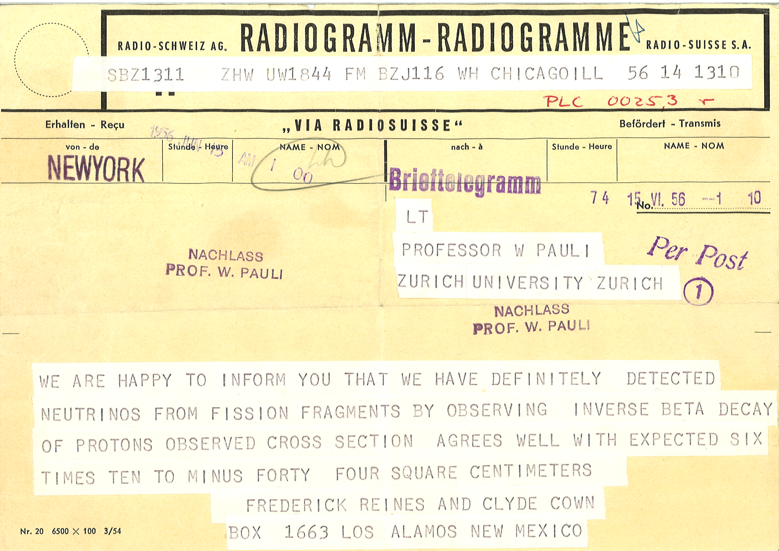
Figure 1.1: Telegram from Fred Reines and Clyde Cowan informing Wolfgang Pauli of their detection of neutrinos from a nuclear reactor.

The first indication of what would come to be known as the neutrino came from Wolfgang Pauli in 1930 [33]. Addressing the “radioactive ladies and gentlemen” of Tübingen, Germany, he appealed to the existence of new electrically neutral particles to save the law of energy conservation in nuclear beta decays. This idea was developed further by Enrico Fermi in 1934, who calculated the transition probability for $\beta$-decay with a neutrino in the final state [34]. Fermi’s theory represents the first study of the weak interaction–the only Standard Model gauge group under which neutrinos are charged.

As the name “weak interaction” suggests, neutrinos interact very feebly with particles in the Standard Model. Thus, it wasn’t until 1956 that the neutrino was observed in an experimental setting for the first time. A team of scientists from Los Alamos Scientific Laboratory, led by Frederick Reines and Clyde Cowan, detected a free neutrino from a nuclear reactor via the inverse beta decay interaction ($\bar{\nu}_{e}p\to e^{+}n$) [35, 36]. Though it was not known at the time, they had detected electron antineutrinos ($\bar{\nu}_{e}$). Electron (anti)neutrinos represent one of the three weak-flavor eigenstates neutrinos can occupy in the Standard Model–specifically, the eigenstate that couples to the $e^{\pm}$ charged leptons through the charged-current weak interaction. Upon confirmation of their discovery, Reines and Cowan sent the telegram shown in figure 1.1 to Pauli, alerting him of the definitive existence of the neutral particles he proposed in Tübingen.

Shortly after this, the phenomenon of neutrino oscillations–periodic transitions between different types of neutrinos–started to appear in the literature. In 1958, Bruno Pontecorvo discussed the possibility of mixing between right-handed antineutrinos $\bar{\nu}_{R}$ and “sterile” right-handed neutrinos $\nu_{R}$, in analogy with $K^{0}$–$\bar{K}^{0}$ mixing observed in the quark sector [37]. A second possible source of neutrino oscillations came following the 1962 experimental discovery of a second neutrino weak-flavor eigenstate–the muon neutrino ($\nu_{\mu}$) [38]. After this, the notion of mixing between neutrino flavor and mass eigenstates was introduced by Ziro Maki, Masami Nakagawa, and Shoichi Sakata [39]. In a 1967 paper [40], Pontecorvo introduced the possibility of vacuum $\nu_{e}$–$\nu_{\mu}$ oscillations, even predicting a factor of two suppression in the total solar neutrino flux before such a deficit would actually be observed [41].

The aforementioned deficit, known as the “solar neutrino problem”, was established in 1968 through a now-famous experiment at the Homestake Mine in South Dakota led by Raymond Davis [42]. Davis and his colleagues detected the capture of electron neutrinos from the sun on ³⁷Cl nuclei, allowing a measurement of the solar $\nu_{e}$ flux. Their result was about a factor of $\sim 1/3$ lower than the leading prediction from John Bachall [43]. This is shown in figure 1.2, including confirmations of the deficit following the Homestake experiment. The solution was not a mistake in the experimental measurement or theoretical prediction, as physicists expected at the time; rather, it was a deficiency in our understanding of neutrinos. This was the first piece of the puzzle that would eventually lead to the discovery of neutrino oscillations and nonzero neutrino masses.

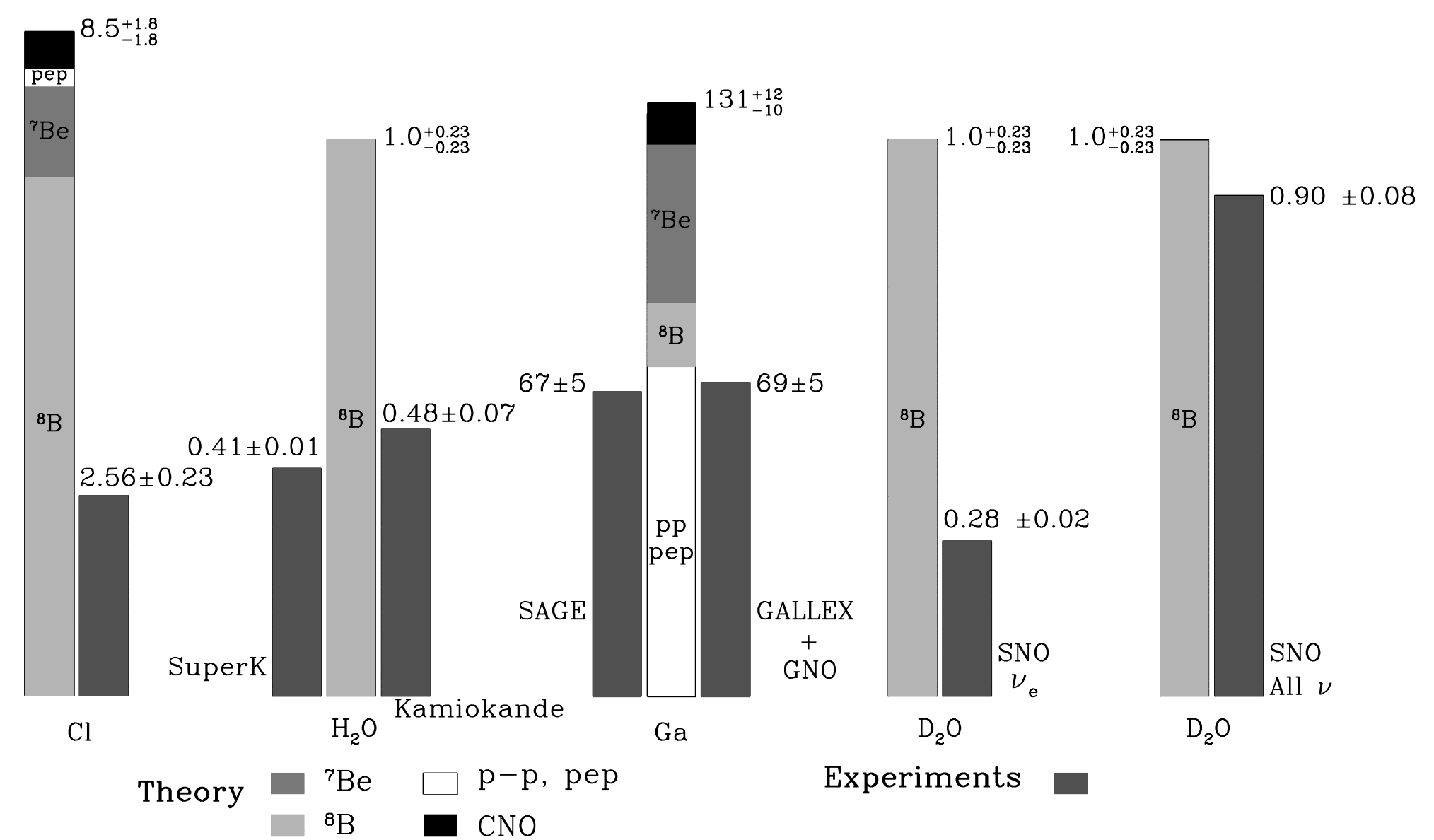
Figure 1.2: The deficit of the observed solar $\nu_{e}$ flux compared with the theoretical expectation. The Homestake experiment is shown on the far left; follow-up solar neutrino measurements confirming the deficit are also shown, including the 2002 SNO result which brought forth a solution to the solar neutrino problem. Figure from Ref. [1].

The next piece of the puzzle came from atmospheric neutrinos, i.e. neutrinos coming from the decay of mesons created from the interactions of primary cosmic rays in the atmosphere. Around the mid-1980s, two water Cherenkov detectors, IMB-3 [44] and Kamiokande [45], began to measure the interactions of atmospheric $\nu_{\mu}$ and $\nu_{e}$ events (initially just as a background for their main physics goal, the search for nucleon decay). The ratio of $\nu_{\mu}:\nu_{e}$ interactions was found to be lower than the theoretical expectation by a factor of $\sim 2/3$ [46]. This was known as the “atmospheric neutrino anomaly”. The source of this anomaly was not clear at the time; it could have been a deficit of muon neutrinos, an excess of electron neutrinos, or some of both. Systematic issues in the flux prediction or muon identification were also suggested [46]. It was far from clear that neutrino oscillations could be responsible for the observed deficit.

The solution to the atmospheric neutrino anomaly came from the Super-Kamiokande (SuperK) experiment [47]. SuperK was a much larger version of the Kamiokande detector, allowing the detection of higher energy muons (up to $E_{\mu}\sim 5\;{\rm GeV}$). SuperK also measured the up-down asymmetry of muon-like and electron-like events in their detector, $(N_{\rm up}-N_{\rm down})/(N_{\rm up}+N_{\rm down})$. Upward-going events have traveled a much longer distance than downward-going events before reaching the SuperK detector–thus positive detection of an asymmetry would be smoking-gun evidence for a baseline-dependent effect like neutrino oscillations. This is precisely what SuperK observed [2]. As shown in figure 1.3, an up-down asymmetry is observed in the muon-like channel, the magnitude of which increases with the observed muon momentum. Such behavior is consistent with muon neutrino oscillations to a third flavor eigenstate, $\nu_{\tau}$ (the mathematical details of neutrino oscillations will be described in section 1.3). No such effect was observed in the electron-like channel. Thus, the atmospheric neutrino anomaly is a result of muon neutrino disappearance, specifically coming from $\nu_{\mu}\to\nu_{\tau}$ oscillations.

The solution to the solar neutrino problem came in 2002 from the Sudbury Neutrino Observatory (SNO) [48]. The SNO experiment used a heavy water Cherenkov detector, specifically relying on the use of deuterium target nuclei to be sensitive to three different neutrino interactions,

$$\begin{split}&\nu_{e}+d\to p+p+e^{-}~{}~{}~{}(\rm{CC}),\\ &\nu_{x}+d\to p+n+\nu_{x}~{}~{}~{}(\rm{NC}),\\ &\nu_{x}+e^{-}\to\nu_{x}+e^{-}~{}~{}~{}~{}~{}(\rm{ES}).\end{split}$$ (1.1)

Charged-current (CC), neutral-current (NC), and elastic scattering (ES) interactions were separated based on the visible energy and scattering angle of the final state particles. NC events were further separated by tagging the 6.25 MeV photon released from neutron capture on deuterium. By measuring all three channels, SNO was able to measure the ⁸B solar neutrino flux broken down into the $\nu_{e}$ and $\nu_{\mu,\tau}$ components. SNO’s 2002 result showed that the missing neutrinos from the Homestake experiment were in fact showing up in the $\nu_{\mu,\tau}$ component [3]. Figure 1.4 shows the flux of each component as constrained by the measured CC, NC, and ES interaction rate. The flavor transitions here come not from vacuum oscillations but rather from matter-enhanced resonant behavior as neutrinos travel through the dense solar medium–a phenomenon known as the Mikheyev–Smirnov–Wolfenstein (MSW) effect [49, 50]. The MSW effect still, however, requires mixing between the neutrino flavor and mass eigenstate as well as non-zero squared differences between the mass eigenstates. It is worth noting here that the KamLAND reactor neutrino experiment was essential in determining the oscillation parameters which led to the SNO observation [51]. Thus, the SNO solution to the solar neutrino problem and the SuperK solution to the atmospheric neutrino anomaly were both evidence for the existence of neutrino oscillations and thus non-zero neutrino masses. The collaborations shared the 2015 Nobel Prize in physics for this discovery [52, 53].

Since SuperK and SNO, neutrino oscillations have been measured extensively by a global program of reactor, accelerator, atmospheric, and solar neutrino experiments. The mixing angle and mass-squared splittings of the three Standard Model neutrinos have been measured to few-percent-level precision in most cases [54, 55, 56]. There are a number of open questions in the standard three-neutrino mixing paradigm, including the ordering of the three mass eigenstates and the value of the charge-parity-violating complex phase $\delta_{CP}$. Though preliminary results exist on both fronts [57, 58, 55, 54, 56], definitive answers to each will come from next-generation neutrino experiments, including Hyper-K [59], DUNE [60] and JUNO [61].

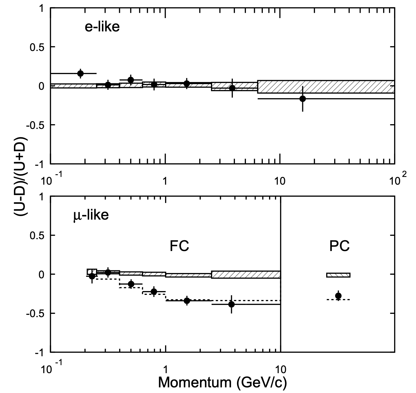
Figure 1.3: The up-down asymmetry measured in SuperK as a function of lepton momentum, separated into $e$-like and $\mu$-like events as well as fully-contained (FC) and partially-contained (PC) events. The dashed line indicates the best fit to $\nu_{\mu}\to\nu_{\tau}$ oscillations. Figure from Ref. [2].

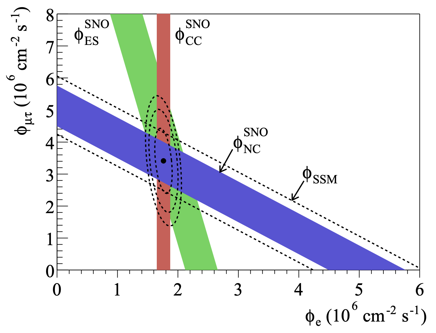
Figure 1.4: Measurement of the solar ⁸B flux from the SNO collaboration, broken down into the $\nu_{e}$ and $\nu_{\mu,\tau}$ sub-components. Measurement of the CC, NC, and ES channels show up as slices in the two-dimensional flux parameter space. Figure from Ref. [3].

1.2 Neutrinos in the Standard Model

The arguments and notation presented in this section follow closely from chapter 2 of Ref. [62].

The interactions of the known fundamental particles of our Universe are described by a specific quantum field theory known as the Standard Model (SM). Above the electroweak scale, there are three gauge groups contained within the SM:

• $SU(3)_{c}$, which governs the gluon-mediated “strong interactions” of color-charged fields.

• $SU(2)_{L}$, one part of the “electro-weak interaction”, mediated by the $W^{\pm}_{\mu}$ and $W^{0}_{\mu}$ vector bosons.

• $U(1)_{Y}$, the other part of the “electro-weak interaction”, mediated by the $B_{\mu}$ gauge boson.

After electro-weak symmetry breaking (EWSB) via the Higgs mechanism, the $SU(2)_{L}\times U(1)_{Y}$ subgroup breaks down to $U(1)_{Q}$, which describes the electromagnetic (EM) interactions of charged fields mediated by the $A_{\mu}$ gauge boson, also known as the photon.

Of the three fundamental interactions of the SM, neutrinos are only charged under the weak $SU(2)_{L}$ gauge group–they are singlets under the $SU(3)_{c}$ and $U(1)_{Q}$ gauge groups. Thus, neutrinos only appear in the electro-weak part of the SM Lagrangian, which is given by

$$\mathcal{L}=\frac{g}{\sqrt{2}}(J^{\mu}W^{+}_{\mu}+J^{\mu\dagger}W^{-}_{\mu})+\frac{g}{\cos\theta_{W}}K^{\mu}Z_{\mu},$$ (1.2)

where $g=e/\cos\theta_{W}$ is the $SU(2)_{L}$ gauge coupling of $W_{\mu}$ and Higgs field, $\theta_{W}$ is the Weinberg angle describing the rotation that occurs during EWSB between the neutral parts of the $SU(2)_{L}$ and $U(1)_{Y}$ gauge boson fields, and $W^{\pm}_{\mu}$ ($Z_{\mu}$) is the charged (neutral) piece of $SU(2)_{L}$ after EWSB. The currents coupled to $W^{\pm}_{\mu}$ and $Z_{\mu}$ bosons are given by

$$\begin{split}J^{\mu}&=\begin{pmatrix}\overline{u}^{0}&\overline{c}^{0}&\overline{t}^{0}\end{pmatrix}\gamma^{\mu}P_{L}\begin{pmatrix}d^{0}\\ s^{0}\\ b^{0}\end{pmatrix}+\begin{pmatrix}\overline{\nu_{e}}&\overline{\nu_{\mu}}&\overline{\nu_{\tau}}\end{pmatrix}\gamma^{\mu}P_{L}\begin{pmatrix}e\\ \mu\\ \tau\end{pmatrix}\\ K^{\mu}&=\sum_{f}\overline{f}\gamma^{\mu}[I_{3L}P_{L}-\sin^{2}\theta_{W}Q_{f}]f\\ &=\sum_{q}[\epsilon_{L}(q)\overline{q}\gamma_{\mu}P_{L}q+\epsilon_{R}(q)\overline{q}\gamma_{\mu}P_{R}q]\\ &+\frac{1}{2}\sum_{\alpha\in\{e,\mu,\tau\}}[\overline{\nu_{\alpha}}\gamma^{\mu}P_{L}\nu_{\alpha}+\overline{\ell}_{\alpha}\gamma_{\mu}(g_{V}^{\alpha}-\gamma_{5}g_{A}^{\alpha})\ell_{\alpha}],\end{split}$$ (1.3)

where $P_{R}(P_{L})=(1\pm\gamma^{5})/2$ is the projection operator onto the right-handed (left-handed) chiral state, and the subscript $0$ on the quark fields indicates that these are the weak flavor eigenstates rather than the mass eigenstates. The first generation coupling constants in $K^{\mu}$, which derive from the specified EM charge and $SU(2)_{L}$ representation of each field, are given by

$$\begin{split}&\epsilon_{L}(u)=\frac{1}{2}-\frac{2}{3}\sin^{2}\theta_{W}~{}~{}~{}~{}~{}\epsilon_{R}(u)=-\frac{2}{3}\sin^{2}\theta_{W}\\ &\epsilon_{L}(d)=-\frac{1}{2}+\frac{1}{3}\sin^{2}\theta_{W}~{}~{}~{}\epsilon_{R}(d)=\frac{1}{3}\sin^{2}\theta_{W}\\ &g_{V}^{e}=-\frac{1}{2}+2\sin^{2}\theta_{W}~{}~{}~{}~{}~{}~{}~{}g_{A}^{e}=-\frac{1}{2}.\end{split}$$ (1.4)

The Lagrangian in equation 1.2 can be used to calculate cross sections for the various SM interactions of the neutrino. The first term describes the charged-current interactions of neutrinos such as nuclear beta decay, while the second term describes neutral current interactions such as $\nu_{\mu}e^{-}$ elastic scattering. At energy scales below the electro-weak scale, one can integrate out the $W_{\mu}$ and $Z_{\mu}$ gauge bosons and describe interactions in terms of the dimensional Fermi constant

$$G_{F}=\frac{g^{2}}{4\sqrt{2}M_{W}^{2}}=1.166\times 10^{-5}\;\rm{GeV}^{-2}.$$ (1.5)

The low-energy Lagrangian describing 4-fermion interactions can be derived from equation 1.2 as

$$\mathcal{L}_{4f}=\frac{-4G_{F}}{\sqrt{2}}[J_{\mu}J^{\mu\dagger}+K_{\mu}K^{\mu}].$$ (1.6)

As an example, we consider low-energy neutrino electron elastic scattering (ES) ($\nu e^{-}\to\nu e^{-}$). This is a purely leptonic process and is therefore relatively clean; specifically, ES models do not need to account for the complex dynamics of the nuclear medium. The Feynman diagrams for the contributing interactions are shown in figure 1.5. Both the charged-current (CC) and neutral-current (NC) diagrams contribute to $\nu_{e}e^{-}$ scattering, while only the NC diagram contributes to $\nu_{\mu,\tau}e^{-}$ scattering. Using the Feynman rules associated with equation 1.6, one can calculate the cross sections to be [62]

$$\begin{split}\sigma_{\nu_{e}e^{-}\to\nu_{e}e^{-}}(E_{\nu})&=\frac{G_{F}^{2}m_{e}E_{\nu}}{2\pi}\bigg{[}(2\sin^{2}\theta_{W}+1)^{2}+\frac{4}{3}\sin^{4}\theta_{W}\bigg{]}\\ &\approx 0.9\times 10^{-43}\bigg{(}\frac{E_{\nu}}{10\;{\rm MeV}}\bigg{)}{\rm cm}^{2}\\ \sigma_{\nu_{\mu,\tau}e^{-}\to\nu_{\mu,\tau}e^{-}}(E_{\nu})&=\frac{G_{F}^{2}m_{e}E_{\nu}}{2\pi}\bigg{[}(2\sin^{2}\theta_{W}-1)^{2}+\frac{4}{3}\sin^{4}\theta_{W}\bigg{]}\\ &\approx 0.15\times 10^{-43}\bigg{(}\frac{E_{\nu}}{10\;{\rm MeV}}\bigg{)}{\rm cm}^{2},\end{split}$$ (1.7)

which is valid for $E_{\nu}>>m_{e}$. Similarly, one can calculate the cross section for antineutrino electron ES ($\overline{\nu}e^{-}\to\overline{\nu}e^{-}$). The diagrams contributing for this process are shown in figure 1.6, and the cross section is given by [62]

$$\begin{split}\sigma_{\overline{\nu}_{e}e^{-}\to\overline{\nu}_{e}e^{-}}(E_{\nu})&=\frac{G_{F}^{2}m_{e}E_{\nu}}{2\pi}\bigg{[}\frac{1}{3}(2\sin^{2}\theta_{W}+1)^{2}+4\sin^{4}\theta_{W}\bigg{]}\\ &\approx 0.378\times 10^{-43}\bigg{(}\frac{E_{\nu}}{10\;{\rm MeV}}\bigg{)}{\rm cm}^{2}\\ \sigma_{\overline{\nu}_{\mu,\tau}e^{-}\to\overline{\nu}_{\mu,\tau}e^{-}}(E_{\nu})&=\frac{G_{F}^{2}m_{e}E_{\nu}}{2\pi}\bigg{[}\frac{1}{3}(2\sin^{2}\theta_{W}-1)^{2}+4\sin^{4}\theta_{W}\bigg{]}\\ &\approx 0.14\times 10^{-43}\bigg{(}\frac{E_{\nu}}{10\;{\rm MeV}}\bigg{)}{\rm cm}^{2}.\end{split}$$ (1.8)

We now turn to the interaction at the core of this thesis: neutrino-nucleon charged-current quasi-elastic (CCQE) scattering. The relevant Feynman diagrams for this process are shown in figure 1.7. Unlike ES, models of CCQE do need to account for the nuclear environment surrounding the target nucleon. As the final state nucleon travels through the nuclear medium, it may scatter off of other nucleons and/or produce additional mesons through a process known as final state interactions (FSIs). As shown in figure 1.8, CCQE is dominant for $E_{\nu}\lesssim 1\;{\rm GeV}$. Above this energy, nucleon resonance processes start to take over, in which Delta resonances decay to final state mesons. In the regime $E_{\nu}\gtrsim 10\;{\rm GeV}$, neutrinos start to undergo deep inelastic scattering (DIS) off of the constituent quarks within the nucleon.

In order to calculate the CCQE cross section, one considers a theory containing nucleon degrees of freedom. The original calculation for free nucleons (i.e., not bound within a nucleus) was carried out by Llewellyn-Smith in 1972; the differential cross section as a function of the squared four-momentum transfer $Q^{2}$ is given by [4, 63]

$$\begin{split}\frac{d\sigma}{dQ^{2}}=\frac{G_{F}^{2}M^{2}|V_{ud}|^{2}}{8\pi E_{\nu}^{2}}\bigg{[}A\pm\frac{s-u}{M^{2}}B+\frac{(s-u)^{2}}{M^{4}}C\bigg{]},\end{split}$$ (1.9)

where +(-) refers to (anti)neutrino scattering, $M$ is the nucleon mass, $m$ is the lepton mass, $(s-u)=4ME_{\nu}-Q^{2}-m^{2}$, and $A$, $B$, and $C$ are functions of the vector, axial-vector, and pseudoscalar form factors of the nucleon (see equations 58, 59, and 60 of Ref. [4] for complete expressions). These form factors describe the composite nature of nucleons under interactions with different Lorentz structures.

For $E_{\nu}<<M$, the $\nu_{e}$ CCQE cross section is approximately [62]

$$\begin{split}\sigma_{\nu_{e}n\to e^{-}p}(E_{\nu})&\approx\frac{G_{F}^{2}E_{\nu}^{2}}{\pi}(g_{V}^{2}+3g_{A}^{2})\\ &\approx 9.75\times 10^{-42}\bigg{[}\frac{E_{\nu}}{10\;{\rm MeV}}\bigg{]}^{2}\;{\rm cm}^{2}.\end{split}$$ (1.10)

In the regime $E_{\nu}\gtrsim 1\;{\rm GeV}$, the $\nu_{e}$ and $\nu_{\mu}$ CCQE cross sections are no longer suppressed by threshold effects and are thus the same, approximately $10^{-38}\;{\rm cm}^{2}$ [4]. This cross section is significantly larger than the elastic scattering and lower energy $\nu_{e}$ CCQE cross sections and is the dominant neutrino interaction for many accelerator-based neutrino experiments, including two at the heart of this thesis: MiniBooNE and MicroBooNE. Finally, we note that the cross section for antineutrino CCQE tends to be smaller; this will be important in chapter 6.

Figure 1.5: Diagrams contributing to $\nu e^{-}$ elastic scattering

Figure 1.6: Diagrams contributing to $\overline{\nu}e^{-}$ elastic scattering

Figure 1.7: Diagrams contributing to neutrino-nucleon charged-current quasielastic scattering

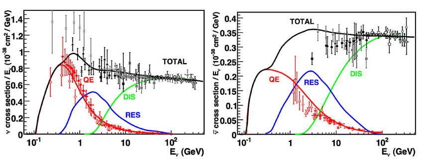
Figure 1.8: CC inclusive neutrino and antineutrino nucleon scattering cross sections as a function of neutrino energy. Figure from Ref. [4].

1.3 Massive Neutrinos

The arguments and notation presented in this section follow closely from section 2.5, chapter 4, and chapter 5 of Ref. [62] as well as chapter 11 of Ref. [64].

Neutrinos are massless in the SM. To see this, we will exhaust the two possible forms for a neutrino mass term in the SM Lagrangian: Dirac and Majorana. These refer to the two possible fermionic spinor representations in which neutrinos can be found. Dirac spinors in general have four complex components, or degrees of freedom, while Majorana spinors have only two. The critical question is whether the right-handed chiral projection of the neutrino field, $\nu_{R}$, is the same as $\overline{\nu}_{R}$, the right-handed chiral projection of the antineutrino field (Majorana case), or if it is a new degree of freedom (Dirac case).

The definition of a free Dirac fermion field is

$$\psi(x)=\int\frac{d^{3}p}{\sqrt{(2\pi)^{3}2E_{p}}}\sum_{s=\pm\frac{1}{2}}\Big{(}f_{s}(\mathbf{p})u_{s}(\mathbf{p})e^{-i\mathbf{p}\cdot\mathbf{x}}+\overline{f_{s}}^{\dagger}(\mathbf{p})v_{s}(\mathbf{p})e^{i\mathbf{p}\cdot\mathbf{x}}\Big{)},$$ (1.11)

where $f_{s}(\mathbf{p})$ annihilates a single particle of momentum $\mathbf{p}$ while $\overline{f_{s}}^{\dagger}$ creates the corresponding antiparticle state, and $u_{s}(\mathbf{p})$ and $v_{s}(\mathbf{p})$ are spinors with positive and negative energy, respectively, satisfying the Dirac equations

$$\begin{split}&(\gamma^{\mu}p_{\mu}-m)u_{s}(\mathbf{p})=0\\ &(\gamma^{\mu}p_{\mu}+m)v_{s}(\mathbf{p})=0,\end{split}$$ (1.12)

where $\gamma^{\mu}$ are a set of Lorentz-indexed matrices satisfying $\{\gamma^{\mu},\gamma^{\nu}\}=2g^{\mu\nu}$. There are many possible representations for the $\gamma$-matrices. We consider the Weyl basis, in which [64]

$$\gamma_{\mu}=\begin{pmatrix}0&\sigma_{\mu}\\ \overline{\sigma}_{\mu}&0\\ \end{pmatrix},$$ (1.13)

where $\sigma_{\mu}=(\mathbb{1},\vec{\sigma})$, $\overline{\sigma}_{\mu}=(\mathbb{1},-\vec{\sigma})$, and $\vec{\sigma}=(\sigma_{1},\sigma_{2},\sigma_{3})$ are the Pauli matrices. This representation is convenient for understanding the different chiral components of the Dirac spinor $\psi$. The Lorentz generators $S^{\mu\nu}\equiv\frac{i}{4}[\gamma^{\mu},\gamma^{\nu}]$ become block diagonal, such that we can write the Dirac spinor of equation 1.11 as a doublet of two-component Weyl spinors with a different chiral nature,

$$\psi=\begin{pmatrix}\psi_{L}\\ \psi_{R}\\ \end{pmatrix},$$ (1.14)

which transform under different irreducible representations of the Lorentz group [64]. Here $\psi_{L}$ and $\psi_{R}$ refer to the left-handed and right-handed Weyl spinor, respectively. We can isolate the different chiral components of the Dirac spinor using the matrix $\gamma^{5}\equiv i\gamma^{0}\gamma^{1}\gamma^{2}\gamma^{3}$, which takes the form

$$\gamma^{5}=\begin{pmatrix}-\mathbb{1}&0\\ 0&\mathbb{1}\\ \end{pmatrix}$$ (1.15)

in the Weyl basis. We can define projection operators $P_{L}=\frac{1}{2}(1-\gamma^{5})$ and $P_{R}=\frac{1}{2}(1+\gamma^{5})$ such that $P_{L}\psi=\psi_{L}$ and $P_{R}\psi_{R}$. It is worth noting that while the behavior of these projection operators is especially clear in the Weyl representation, they will isolate the chiral components of $\psi$ in any representation of $\gamma^{\mu}$.

Dirac mass terms couple left-handed and right-handed chiral states. To see this, consider the Dirac equation in the Weyl basis, which takes the form [64]

$$(\gamma^{\mu}p_{\mu}-m)\psi=\begin{pmatrix}-m&\sigma^{\mu}p_{\mu}\\ \overline{\sigma}^{\mu}p_{\mu}&-m\\ \end{pmatrix}\begin{pmatrix}\psi_{L}\\ \psi_{R}\\ \end{pmatrix}=0.$$ (1.16)

It is evident that this matrix equation mixes the left-handed and right-handed components of $\psi$. Dirac mass terms take the form $m\psi_{L}^{\dagger}\psi_{R}$ and $m\psi_{R}^{\dagger}\psi_{L}$, thus requiring both chiral components. After EWSB, the non-neutrino fermions in the SM acquire a Dirac mass from their interactions with the Higgs field. Neutrinos, however, do not have a right-handed chiral state in the SM; therefore, the SM cannot include a Dirac mass term for neutrinos.

Now we turn to the Majorana mass term. The expression for a Majorana field is the same as equation 1.11, subject to a condition relating particles and antiparticles. We see that the expression for $\psi^{*}(x)$ would involve $f_{s}^{\dagger}(\mathbf{p})$, which creates a particle state, and $\overline{f_{s}}(\mathbf{p})$, which annihilates an antiparticle state. It turns out the relationship $\psi(x)=\psi^{*}(x)$ is not Lorentz invariant [62]. To remedy this, we must define the conjugate Dirac field

$$\psi^{C}(x)\equiv\gamma_{0}C\psi^{*}(x),$$ (1.17)

where the representation-dependent conjugation matrix $C$ is defined by the equation

$$\begin{split}&\gamma_{0}C\sigma^{*}_{\mu\nu}=-\sigma_{\mu\nu}\gamma_{0}C,\\ &\sigma_{\mu\nu}\equiv\frac{i}{2}[\gamma_{\mu},\gamma_{\nu}].\end{split}$$ (1.18)

In the Weyl representation, for example, $C=i\gamma_{2}\gamma_{0}$. This requirement for $C$ ensures that $\psi^{C}(x)$ transforms in the same way as $\psi(x)$ under the Lorentz group [62]. The Lorentz-invariant Majorana condition specifically requires

$$\psi(x)=e^{i\theta}\psi^{C}(x),$$ (1.19)

where $\theta$ is an arbitrary phase, which we can take to be $\theta=0$. It is important to note that this condition can only be satisfied for fields that carry no additive quantum numbers [64].

In the Weyl basis, equation 1.19 relates the left-handed and right-handed components of $\psi(x)$ such that [64]

$$\psi(x)=\begin{pmatrix}\psi_{L}\\ i\sigma_{2}\psi^{*}_{L}\\ \end{pmatrix},$$ (1.20)

where the number of degrees of freedom has been reduced from four to two. Since $i\sigma_{2}\psi^{*}_{L}$ transforms like a right-handed spinor, we can now write mass terms of the form $im\psi_{L}^{\dagger}\sigma_{2}\psi_{L}^{*}$ and $im\psi_{L}^{\dagger}\sigma_{2}\psi_{L}^{*}$. These are Majorana mass terms. Note that they couple the same chiral component of the fermion.

The impossibility of a neutrino Majorana mass term is a bit more nuanced. Majorana mass terms for neutrinos in the SM contain the bi-linear expression $\nu_{L}^{T}\sigma_{2}\nu_{L}$. However, $\nu_{L}$ belongs to an $SU(2)_{L}$ doublet in the SM, thus this Majorana mass term transforms as a triplet under $SU(2)_{L}$. It also breaks lepton number by two units, hence it also violates baryon minus lepton number ($B-L$), which is conserved to all orders of the SM gauge couplings [62]. Therefore, neutrinos also cannot have a Majorana mass term in the SM.

Despite these arguments, neutrino oscillations have given physicists definitive evidence that at least two of the three SM neutrino masses are nonzero (as discussed in section 1.1). This requires the presence of physics beyond the Standard Model (BSM). The minimal extension of the SM which can accommodate nonzero neutrino masses introduces additional right-handed neutrino states $N_{R}$ [62, 64]. These fields, which are singlets under the SM gauge group, can generate both Dirac and Majorana mass terms for neutrinos. The most general expression for the neutrino mass Lagrangian is then

$$-\mathcal{L}_{\rm mass}=\frac{1}{2}\begin{pmatrix}\overline{\nu}_{L}&\overline{N^{C}_{L}}\end{pmatrix}\begin{pmatrix}0&M\\ M^{T}&B\\ \end{pmatrix}\begin{pmatrix}\nu_{R}^{C}\\ N_{R}\end{pmatrix}+{\rm h.c.},$$ (1.21)

where $M$ and $B$ are the Dirac and Majorana mass matrices of the neutrino sector, respectively, and $\nu_{L}$ and $N_{R}$ are column vectors containing the left-handed and right-handed projections of each neutrino generation.

In order to obtain the mass eigenstates of this theory, one must diagonalize the mass matrix in equation 1.21. If we assume one generation of neutrinos, the eigenvalues of this mass matrix are

$$m_{1,2}=\frac{1}{2}(\sqrt{B^{2}+4M^{2}}\mp B).$$ (1.22)

In the limit $B>>M$, the eigenvalues are approximately given by

$$m_{1}\approx\frac{M^{2}}{B},~{}~{}~{}m_{2}\approx B.$$ (1.23)

This is the famous “seesaw mechanism” for neutrino mass generation [65]. One can see that if $B$ is at roughly the GUT scale ($10^{16}$ GeV) and $M$ is at roughly the electro-weak scale (100 GeV), we see that $m_{1}<1$ eV. This is the right order-of-magnitude regime predicted by neutrino oscillation data and is consistent with existing upper bounds on the neutrino mass from KATRIN [66]. Thus, this model is an elegant explanation of the observed neutrino oscillation phenomenon, though experimental confirmation of right-handed neutrino fields at the GUT scale is probably not feasible for quite a long time.

While we do not know the mechanism through which neutrinos acquire mass, it is relevant to ask whether the resulting mass terms are Dirac or Majorana in nature. An extensive worldwide experimental program is currently underway to answer this question by searching for neutrino-less double beta decay, a rare decay process in which a nucleus undergoes two simultaneous beta decays without emitting any neutrinos in the final state [67, 68, 69]. A positive observation would imply that neutrinos are Majorana.

As discussed in section 1.1, perhaps the most famous consequence of massive neutrinos is the phenomenon of neutrino oscillations [37, 40, 39]. This arises because the three weak flavor eigenstates $\nu_{\alpha}$ are not aligned with the three mass eigenstates $\nu_{i}$. The two bases are related by the unitary Pontecorvo–Maki–Nakagawa–Sakata (PMNS) mixing matrix $U_{\alpha i}$,

$$\begin{pmatrix}\nu_{e}\\ \nu_{\mu}\\ \nu_{\tau}\end{pmatrix}=\begin{pmatrix}U_{e1}&U_{e2}&U_{e3}\\ U_{\mu 1}&U_{\mu 2}&U_{\mu 3}\\ U_{\tau 1}&U_{\tau 2}&U_{\tau 3}\\ \end{pmatrix}\begin{pmatrix}\nu_{1}\\ \nu_{2}\\ \nu_{3}\end{pmatrix}.$$ (1.24)

As seen in equation 1.2, neutrinos interact in the weak flavor eigenstates $\nu_{\alpha}$. Thus, a neutrino a produced alongside a charged anti-lepton $\overline{\ell}$ is in the state

$$\ket{\nu(t=0)}=\ket{\nu_{\ell}}=\sum_{i\in\{1,2,3\}}U_{\ell i}\ket{\nu_{i}}.$$ (1.25)

Neutrinos propagate, however, in their mass eigenstates. Each mass eigenstate $\nu_{i}$ is associated with a mass $m_{i}$ and four-momentum $(p_{i})_{\mu}=(E_{i},\vec{p_{i}})$ satisfying the on-shell requirement $(p_{i})^{2}=m_{i}^{2}$. Thus, after a time $t$, the neutrino will be in the state

$$\ket{\nu(t)}=\sum_{i}e^{-ip_{i}\cdot x}U_{\ell i}\ket{\nu_{i}}.$$ (1.26)

The overlap with a different weak flavor eigenstate $\nu_{\ell^{\prime}}\neq\nu_{\ell}$ is non-trivial, given by the expression

$$\begin{split}\braket{\nu_{\ell^{\prime}}}{\nu(t)}&=\sum_{i,j}\bra{\nu_{j}}U^{\dagger}_{j\ell^{\prime}}e^{-ip_{i}\cdot x}U_{\ell i}\ket{\nu_{i}}\\ &=\sum_{i}e^{-ip_{i}\cdot x}U_{\ell i}U_{\ell^{\prime}i}^{*},\end{split}$$ (1.27)

where we have invoked the orthonormality of the mass basis in the last line. The probability of finding a neutrino in flavor eigenstate $\nu_{\ell^{\prime}}$ given an initial $\nu_{\ell}$ state is then

$$\begin{split}P_{\nu_{\ell}\to\nu_{\ell^{\prime}}}(t)&=|\braket{\nu_{\ell}^{\prime}}{\nu(t)}|^{2}\\ &=\sum_{i,j}|U_{\ell i}U_{\ell^{\prime}i}^{*}U_{\ell j}^{*}U_{\ell^{\prime}j}|e^{-i(p_{i}-p_{j})\cdot x+i\phi_{\ell\ell^{\prime}ij}}.\end{split}$$ (1.28)

where $\phi_{\ell\ell^{\prime}ij}\equiv\rm{arg}(U_{\ell i}U_{\ell^{\prime}i}^{*}U_{\ell j}^{*}U_{\ell^{\prime}j})$.

We now make a simplifying assumption, in which all neutrino mass eigenstates propagate with the same momentum, i.e. $\vec{p}_{i}=\vec{p}_{j}\equiv\vec{p}\forall i,j$. This treatment is not necessarily physical. However, for the parameters relevant to most laboratory neutrino experiments, it leads to the same result as the correct but complicated full treatment of the quantum mechanical neutrino wave packet [70]. Given this assumption along with the approximation that $m_{i}<<p_{i}$ (which should hold for all existing and near-future experiments), we can show

$$\begin{split}(p_{i}-p_{j})\cdot x&=(E_{i}-E_{j})t\\ &=\Big{(}\sqrt{\vec{p}^{2}+m_{i}^{2}}-\sqrt{\vec{p}^{2}+m_{j}^{2}}\Big{)}t\\ &\approx\frac{\Delta m_{ij}^{2}t}{2|\vec{p}|},\end{split}$$ (1.29)

where $\Delta m_{ij}^{2}=m_{i}^{2}-m_{j}^{2}$. Working in natural units ($c=\hbar=1$), we note that ultra-relativistic neutrinos satisfy $|\vec{p}|\approx E$ and $t\approx L$, where $L$ is the distance traveled by the neutrino. Taking only the real part of the exponential in equation 1.28, we have

$$P_{\nu_{\ell}\to\nu_{\ell^{\prime}}}(t)=\sum_{i,j}|U_{\ell i}U_{\ell^{\prime}i}^{*}U_{\ell j}^{*}U_{\ell^{\prime}j}|\cos\Big{(}\frac{\Delta m_{ij}^{2}L}{2E}-\phi_{\ell\ell^{\prime}ij}\Big{)}.$$ (1.30)

If we consider a two-neutrino paradigm, the unitary mixing matrix is real and can be parameterized by a single “mixing angle” $\theta$,

$$U\equiv\begin{pmatrix}U_{\ell 1}&U_{\ell 2}\\ U_{\ell^{\prime}1}&U_{\ell^{\prime}2}\end{pmatrix}=\begin{pmatrix}\cos\theta&\sin\theta\\ -\sin\theta&\cos\theta\end{pmatrix}.$$ (1.31)

In this scenario, summing over the two mass eigenstates as in equation 1.30 gives

$$P_{\nu_{\ell}\to\nu_{\ell^{\prime}}}(t)=\sin^{2}2\theta\sin^{2}\Big{(}\frac{\Delta m^{2}L}{4E}\Big{)}.$$ (1.32)

The extension to the standard three neutrino paradigm can be found in any text on neutrino oscillations. We quote the result here. Three mass eigenstates lead to two independent mass-squared splittings, $\Delta m_{12}^{2}$ and $\Delta m_{23}^{2}$. The mixing matrix in equation 1.24 can be parameterized by three real mixing angles $\theta_{ij}$ and one complex CP-violating phase $\delta$,

$$U=\begin{pmatrix}1&0&0\\ 0&c_{23}&s_{23}\\ 0&-s_{23}&c_{23}\\ \end{pmatrix}\begin{pmatrix}c_{13}&0&s_{13}e^{-i\delta}\\ 0&1&0\\ -s_{13}e^{i\delta}&0&c_{13}\\ \end{pmatrix}\begin{pmatrix}c_{12}&s_{12}&0\\ -s_{12}&c_{12}&0\\ 0&0&1\\ \end{pmatrix}$$ (1.33)

where $c_{ij}\equiv\cos\theta_{ij}$ and $s_{ij}\equiv\sin\theta_{ij}$. The three mixing angles ($\theta_{12}$, $\theta_{13}$, $\theta_{23}$) and two relevant mass squared splittings $\Delta m_{12}^{2}$ and $|\Delta m_{23}^{2}|$ have been measured to a precision of $\mathcal{O}(1\%-10\%)$ over the past two decades [54, 55, 56]. An extensive experimental program is planned to measure $\delta$ to similar precision, as well as the neutrino hierarchy (i.e., the sign of $\Delta m_{23}^{2}$) and the octant of $\theta_{23}$ [71].

1.4 Anomalies in the Neutrino Sector

Despite the success of the three-neutrino mixing paradigm, several anomalous results have appeared. Perhaps the most famous of these is the excess of $\bar{\nu}_{e}$ candidate events observed by the Liquid Scintillator Neutrino Detector (LSND) experiment [5]. LSND took data at Los Alamos Meson Physics Facility (LAMPF) from 1993-1998, observing neutrino interactions from a high-intensity decay-at-rest (DAR) source. The LSND detector was a 167-ton cylindrical tank of mineral oil that collected scintillation and Cherenkov light produced in neutrino interactions. The LAMPF accelerator provided a $\sim 1\;{\rm mA}$ beam of 798 MeV protons, which were then focused on a water or high-Z target. This process created a large number of pions, which then decayed to produce neutrinos. Most $\pi^{-}$ came to rest and were captured by nuclei in and around the target, and the $\pi^{+}\to\nu_{e}e^{+}$ decay chain is helicity-suppressed due to the interplay between angular momentum conservation and the left-chiral nature of the weak interaction. Thus the dominant neutrino production process was $\pi^{+}\to\nu_{\mu}(\mu^{+}\to\bar{\nu}_{\mu}\nu_{e}e^{+})$.

LSND looked specifically for $\bar{\nu}_{\mu}\to\bar{\nu}_{e}$ conversion using $\bar{\nu}_{\mu}$ from $\mu^{+}$ DAR. The $\bar{\nu}_{e}$ events were observed via the inverse beta decay (IBD) process. This is a very clean channel, as one can require a coincidence between the initial positron emission and the subsequent neutron capture on hydrogen, which releases a characteristic $2.2\;{\rm MeV}$ photon. The intrinsic $\bar{\nu}_{e}$ flux, coming predominately from $\pi^{-}$ decay-in-flight (DIF), was suppressed compared to intrinsic $\bar{\nu}_{\mu}$ by a factor of $\sim 8\times 10^{-4}$. Any significant excess of $\bar{\nu}_{e}$ would be evidence for $\bar{\nu}_{\mu}\to\bar{\nu}_{e}$ oscillations. This is exactly what LSND observed, as shown in figure 1.9. However, the neutrino energies $\mathcal{O}(30\;{\rm MeV})$ and baselines $(\mathcal{O}(30\;{\rm m})$ required a mass-squared-splitting of $\Delta m^{2}\sim 1\;{\rm eV^{2}}$. This is larger than the measured values of $\Delta m^{2}_{12}$ and $|\Delta m^{2}_{23}|$ by at least three orders of magnitude–therefore, the LSND result cannot be explained by the standard three neutrino oscillation paradigm. One must introduce a fourth neutrino to the SM neutrinos in order to facilitate such oscillations. Measurements of the invisible width of the $Z$ boson forbid this neutrino from coupling to the weak force in the same way as the three SM neutrinos [72]. Thus, this fourth neutrino is typically referred to as a “sterile neutrino” ($\nu_{s}$). The sterile neutrino paradigm will be introduced in more detail in section 1.4 and discussed thoroughly throughout this thesis. The LSND anomaly is currently under direct investigation by the follow-up JSNS² experiment [73, 74], which will use a gadolinium-loaded liquid scintillator detector [75] to measure IBD interactions at the J-PARC Materials and Life Science Experimental Facility.

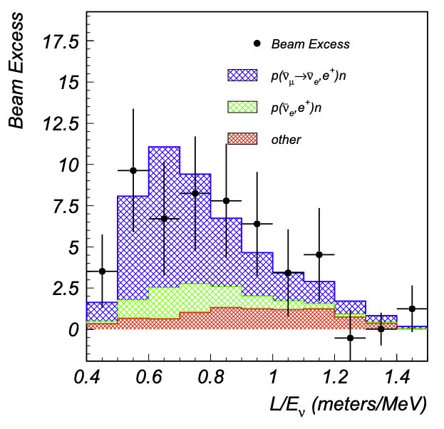
Figure 1.9: The LSND excess of $\overline{\nu}_{e}$ events on top of the predicted SM background (green and red regions). The blue region indicates the best fit to $\overline{\nu}_{\mu}\to\overline{\nu}_{e}$ oscillations via a sterile neutrino state. Figure from Ref. [5]

The Mini Booster Neutrino Experiment (MiniBooNE) was designed to follow up on the LSND anomaly [76]. MiniBooNE took data at Fermilab’s Booster Neutrino Beam (BNB) from 2002-2019, observing the interactions of neutrinos with energy $E\sim 500\;{\rm MeV}$ in an 800-metric-ton mineral oil (CH₂) detector [15]. The Fermilab Booster accelerates protons to a kinetic energy of 8 GeV, at which point they collide with the beryllium target of the BNB. This produces a cascade of mesons, predominately pions. The charged mesons are focused using a magnetic horn and decay in a 50 m decay pipe; in the nominal “neutrino mode”, the magnetic field is generated to create a flux of mostly muon neutrinos from $\pi^{+}$ decay-in-flight [14]. The current in the magnetic horns can be reversed to instead focus $\pi^{-}$ along the beamline, thus creating a beam of mostly muon antineutrinos–this is referred to as “antineutrino mode”. MiniBooNE was situated at a baseline of $L\sim 500\;{\rm m}$ from the BNB target, resulting in a similar characteristic $L/E$ as that of LSND, $\approx 1\;{\rm m/MeV}$. By equation 1.30, this means MiniBooNE would also be sensitive to oscillations at $\Delta m^{2}\sim 1\;{\rm eV}^{2}$.

In 2007, MiniBooNE began to report results from their flagship analysis: the search for an excess of $\nu_{e}$ events in the BNB [76]. MiniBooNE relied primarily on the reconstruction of Cherenkov light from charged final state particles to identify neutrino interactions. Thus, $\nu_{e}$ CC interactions would show up as a “fuzzy” Cherenkov ring due to multiple scattering of the electron as well as the induced EM shower [77]. These fuzzy Cherenkov ring events are hereafter referred to as “electron-like” events. Starting with the initial results [76, 78], MiniBooNE has consistently observed an excess of electron-like events above their expected SM background, the significance of which has grown over the 17-year data-taking campaign of the experiment [10]. Figure 2.5 shows the $4.8\sigma$ MiniBooNE electron-like excess considering the total neutrino mode dataset, corresponding to $18.75\times 10^{20}$ protons-on-target (POT) [10]. A similar excess was observed in the antineutrino mode dataset [79]. The as-yet-unexplained MiniBooNE excess represents one of the most significant disagreements with the SM to date.

Though the origin of the MiniBooNE excess remains unknown, neutrino physicists have converged on a number of potential explanations. The most famous explanation involves sterile neutrino-driven $\nu_{\mu}\to\nu_{e}$ oscillations consistent with the LSND result ($\Delta m^{2}\sim 1\;{\rm eV^{2}}$). While this model can explain at least some of the MiniBooNE excess, the excess in the lowest energy region ($E_{\nu}\lesssim 400\;{\rm MeV}$) sits above even the best-fit sterile neutrino solution. Due to the Cherenkov nature of the detector, electrons and photons are essentially indistinguishable–both seed EM showers which appear as fuzzy Cherenkov rings. Thus, the MiniBooNE excess could also come from a mismodeled photon background. Though not the subject of this thesis, there have been extensive experimental and theoretical efforts, both within and outside of the MiniBooNE collaboration, to validate the MiniBooNE SM photon background prediction [10, 80, 81, 82]. One can also consider BSM sources of electron-like events in MiniBooNE. Typical models introduce additional sources of photons and/or $e^{+}e^{-}$ events in MiniBooNE through couplings to new dark sector particles. Resolution of the LSND and MiniBooNE anomalies, often referred to as the short baseline (SBL) anomalies, is a major goal within the particle physics community [83]. This thesis specifically investigates the MiniBooNE anomaly in further detail, covering both experimental and phenomenological studies into the origin of the excess.

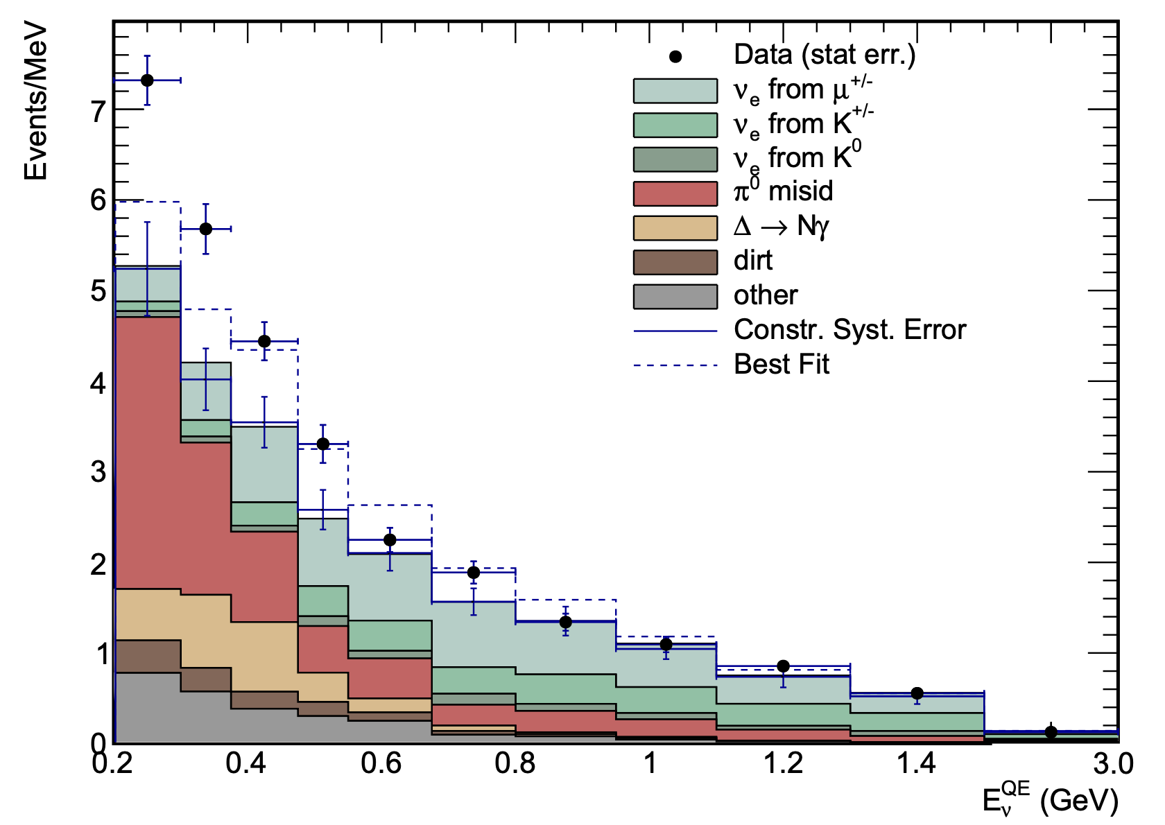
Figure 1.10: The MiniBooNE electron-like channel data and SM background prediction for the entire neutrino mode dataset, as a function of the reconstructed neutrino energy.

We now briefly touch on two additional classes of anomalies that have surfaced over the years: the reactor antineutrino anomaly (RAA) and the gallium anomaly. The RAA [8] is a $\sim 5\%$ deficit in the total $\overline{\nu}_{e}$ rate observed from nuclear reactors compared to the theoretical expectation from the Huber-Mueller (HM) model [84, 85]. The HM model combines results using the summation method (summing the contributions of all beta-decay branches in the reactor) and the conversion method (relying on older measurements of the $\overline{\nu}_{e}$ flux from the different fissionable isotopes in the reactor). The data contributing to the RAA mostly come from reactor neutrino experiments operating at baselines short enough that the effects of SM neutrino oscillations are negligible. One can interpret the RAA as due to $\overline{\nu}_{e}$ disappearance via oscillations involving a sterile neutrino. Coincidentally, due to the relevant neutrino energies and baselines, such a solution requires $\Delta m^{2}\gtrsim 1\;{\rm eV}^{2}$, similar to the LSND and MiniBooNE solution [6]. Figure 1.11 shows an overview of the RAA circa 2012, including the suite of short baseline reactor experiments which observe a deficit with respect to the HM model with SM neutrino oscillations (red line), as well as an example sterile neutrino solution to the RAA (blue line). Recently, the reactor $\overline{\nu}_{e}$ flux calculation has been revisited by various groups, each of which improves upon some aspect of the summation or conversion method used in the HM flux model [86, 87, 88, 89]. The significance of the RAA either diminishes or disappears in some of these models; however, these improved models have difficulty removing the RAA while also explaining the “5-MeV bump” observed by most short baseline reactor experiments with respect to the HM model [89]. Thus, while the RAA story is quickly evolving, our understanding of reactor neutrino fluxes is far from clear.

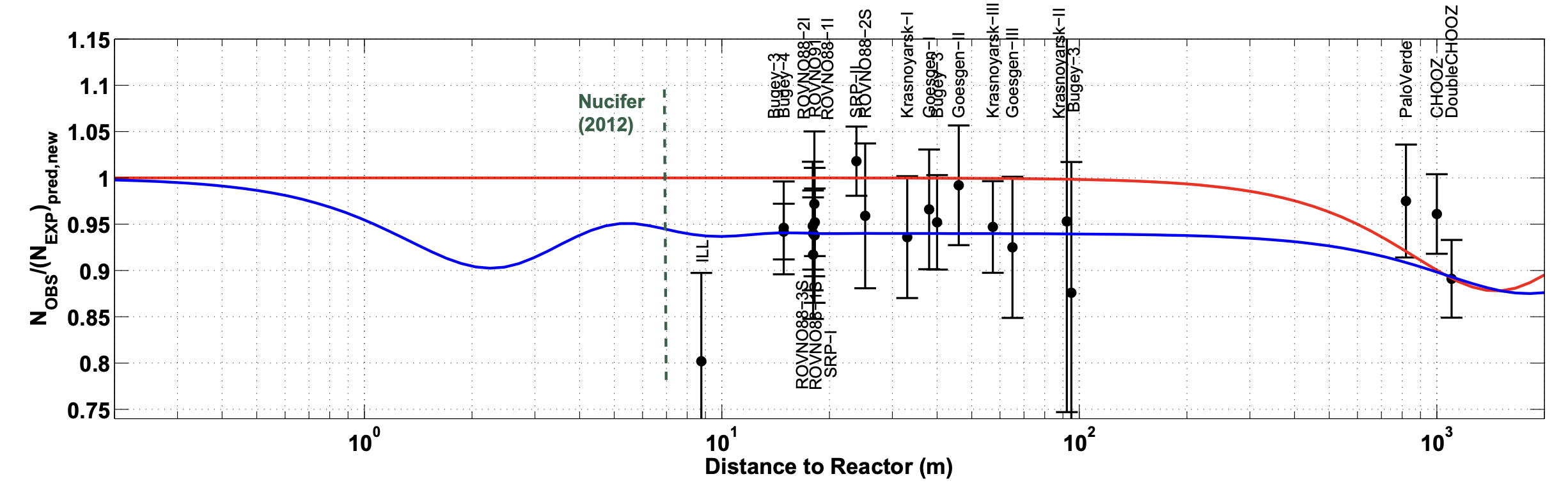
Figure 1.11: Data contributing to the reactor antineutrino anomaly, indicating the $\sim 5\%$ flux deficit observed by short-baseline reactor neutrino experiments. The red line indicates the prediction incorporating SM neutrino oscillations only, while the blue line shows an example prediction including a sterile neutrino. Figure from Ref. [6].

The gallium anomaly refers to a series of gallium-based detectors that have observed a deficit of $\nu_{e}$ capture events on ⁷¹Ga with respect to the theoretical expectation. The original harbingers of the anomaly, SAGE [90] and GALLEX [91], were designed to measure solar neutrinos using the ${}^{71}{\rm Ga}\nu_{e}\to{}^{71}{\rm Ge}e^{-}$ capture process. Each detector was calibrated using electron capture $\nu_{e}$ sources, including ⁵¹Cr and ³⁷Ar. Combining all available calibration data across both experiments, the observed ⁷¹Ge production rate was lower than the expectation by a factor of $0.87\pm 0.05$ [90]. Though the statistical significance of the anomaly was only modest ($2-3\sigma$), the community was already beginning to interpret the anomaly as $\nu_{e}\to\nu_{s}$ transitions via an eV-scale sterile neutrino [92]. A follow-up experiment to the SAGE and GALLEX anomaly, BEST [9], released their first results in 2021. BEST placed a 3.414 MCi ⁵¹Cr $\nu_{e}$ source at the center of two nested ⁷¹Ga volumes, each with a different average distance from the source. The ratio of observed to the predicted ⁷¹Ge production rate was $R_{in}=0.79\pm 0.05$ ($R_{out}=0.77\pm 0.05$) for the inner (outer) volume, thus reaffirming the gallium anomaly [9]. No evidence for a difference in the deficit between the inner and outer volumes was observed, which would have been a smoking gun signature of a baseline-dependent effect like $\nu_{e}\to\nu_{s}$ oscillations. However, the statistical significance of the gallium anomaly is now much stronger; the combined SAGE, GALLEX, and BEST results give evidence for a deficit at the $5.0\sigma$ level [7]. The datasets contributing to this anomaly are summarized in figure 1.12.

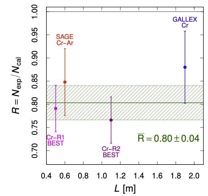
Figure 1.12: Data contributing to the gallium anomaly, indicating the $\sim 20\%$ deficit in the ⁷¹Ge production rate observed by SAGE, GALLEX, and BEST. Figure from Ref. [7].

As alluded to above, the most common BSM interpretation of the SBL, reactor antineutrino, and gallium anomalies is the “3+1 model”, which involves the addition of a new neutrino state–the sterile neutrino–at the eV scale. The sterile neutrino introduces a fourth weak interaction eigenstate $\nu_{s}$ and mass eigenstate $\nu_{4}$ to the standard three-neutrino mixing paradigm. Thus, equation 1.24 becomes

$$\begin{pmatrix}\nu_{e}\\ \nu_{\mu}\\ \nu_{\tau}\\ \nu_{s}\end{pmatrix}=\begin{pmatrix}U_{e1}&U_{e2}&U_{e3}&U_{e4}\\ U_{\mu 1}&U_{\mu 2}&U_{\mu 3}&U_{\mu 4}\\ U_{\tau 1}&U_{\tau 2}&U_{\tau 3}&U_{\tau 4}\\ \end{pmatrix}\begin{pmatrix}\nu_{1}\\ \nu_{2}\\ \nu_{3}\\ \nu_{4}\end{pmatrix}.$$ (1.34)

As we are interested in an eV-scale sterile neutrino, the mass-squared splittings between the three active neutrinos are smaller by at least 2-3 orders of magnitude compared to their mass-squared splittings with the fourth mass eigenstate. This means that the active neutrino mass splittings are negligible for short-baseline experiments, i.e. those in which the argument of the second $\sin^{2}$ term in equation 1.32 is small. Experiments contributing to the aforementioned anomalies all satisfy this condition. Thus, when considering sterile neutrino explanations for these anomalies, we can make the approximation

$$\Delta m^{2}_{41}\approx\Delta m^{2}_{42}\approx\Delta m^{2}_{43}\equiv\Delta m^{2},$$ (1.35)

where we hereafter use $\Delta m^{2}$ to refer to the mass-squared splitting of the fourth mass eigenstate. This approximation holds regardless of the hierarchy of SM neutrino mass eigenstates.

The experiments discussed in this thesis are sensitive only to $\overset{\textbf{(---)}}{\nu}_{e}$ and $\overset{\textbf{(---)}}{\nu}_{\mu}$ interactions. The sterile neutrino can facilitate short-baseline oscillations between these flavor states; the oscillation probability expressions, which can be derived using equation 1.30 within the 3+1 framework, are given by [93]

$$\begin{split}&P_{\nu_{e}\to\nu_{e}}=1-4\sin^{2}2\theta_{ee}\sin^{2}(1.27\Delta m^{2}L/E)\\ &P_{\nu_{\mu}\to\nu_{\mu}}=1-4\sin^{2}2\theta_{\mu\mu}\sin^{2}(1.27\Delta m^{2}L/E)\\ &P_{\nu_{\mu}\to\nu_{e}}=4\sin^{2}2\theta_{\mu e}\sin^{2}(1.27\Delta m^{2}L/E),\end{split}$$ (1.36)

where $\Delta m^{2}$, $L$, and $E$ are in units of eV², km, and GeV, respectively, and

$$\begin{split}&\sin^{2}2\theta_{ee}=4(1-|U_{e4}|^{2})|U_{e4}|^{2}\\ &\sin^{2}2\theta_{\mu\mu}=4(1-|U_{\mu 4}|^{2})|U_{\mu 4}|^{2}\\ &\sin^{2}2\theta_{\mu e}=4|U_{\mu 4}|^{2}|U_{e4}|^{2}.\end{split}$$ (1.37)

The first expression in equation 1.36 can potentially explain the deficit of $\overline{\nu}_{e}$ and $\nu_{e}$ events observed in the RAA and gallium anomaly, respectively. Though both anomalies stem qualitatively from the same phenomenon–$\overset{\textbf{(---)}}{\nu}_{e}$ disappearance at short baseline–the gallium anomaly in general prefers a larger value of $\sin^{2}2\theta_{ee}$ than the RAA. This is evident in figure 1.13, which shows the regions in $\sin^{2}2\theta_{ee}$–$\Delta m^{2}$ parameter space preferred by the RAA and gallium anomalies, as well as global constraints from other experiments. These constraints come from short-to-medium-baseline reactor experiments, including NEOS [94], RENO [95], and Daya Bay [96], as well as very-short-baseline reactor experiments, including STEREO [97], DANSS [98], and PROSPECT [99]. Each of these experiments searches for $\overline{\nu}_{e}$ disappearance in a reactor-flux-agnostic way: the former though comparisons of the reactor $\overline{\nu}_{e}$ spectra measured by different detectors [100], and the latter through the use of modular or movable detectors capable of comparing $\overline{\nu}_{e}$ interaction rates across different baselines. The KATRIN experiment, which is sensitive to the neutrino mass via an extremely precise measurement of the tritium beta spectrum endpoint, also places strong constraints on $\sin^{2}2\theta_{ee}$ in the $\Delta m^{2}\gtrsim 10~{}{\rm eV}^{2}$ region [101].

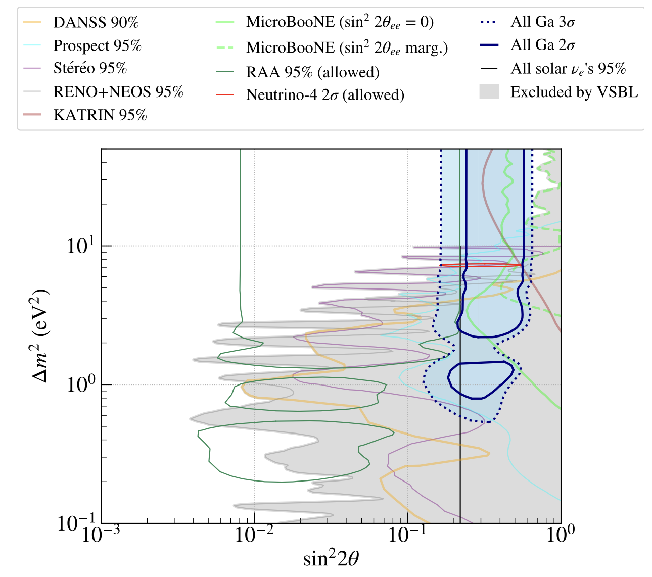
Figure 1.13: Preferred regions in $\sin^{2}2\theta_{ee}$–$\Delta m^{2}$ parameter space to explain the RAA [8] (green contour) and gallium anomaly [9] (blue regions). The total excluded region from other experiments (grey region) is also shown. Figure from Ref. [9].

The second expression in equation 1.36 can potentially explain the SBL anomalies. This is because both LSND and MiniBooNE operated at accelerator neutrino sources for which the neutrino flux was generated mainly by charged pion decay [5, 14]; thus, due to helicity suppression, the flavor composition was dominated muon-flavored (anti)neutrinos. This means that even a small value of $\sin^{2}2\theta_{\mu e}$ could generate an observable level of $\overset{\textbf{(---)}}{\nu}_{e}$ appearance on top of the SM $\overset{\textbf{(---)}}{\nu}_{e}$ flux prediction. Figure 1.14 shows the allowed regions in $\sin^{2}2\theta_{\mu e}$–$\Delta m^{2}$ parameter space from LSND and MiniBooNE [10]. Strikingly, both anomalies generally prefer the same region of parameter space. However, as the MiniBooNE excess tends to peak more sharply at lower energies, the 3+1 fit prefers lower values of $\Delta m^{2}$ compared to the LSND result.

It is important to note that the fits performed in figure 1.14 account only for $\overset{\textbf{(---)}}{\nu}_{\mu}\to\overset{\textbf{(---)}}{\nu}_{e}$ oscillations, ignoring any potential $\overset{\textbf{(---)}}{\nu}_{e}$ or $\overset{\textbf{(---)}}{\nu}_{\mu}$ disappearance in the SM background prediction. This is a reasonable approximation, however, the inclusion of the latter effects does indeed impact the MiniBooNE allowed regions. This effect was only accounted for recently in Ref. [102], which is presented in section 5.3.1 of this thesis.

Figure 1.14: Preferred regions in $\sin^{2}2\theta_{\mu e}$–$\Delta m^{2}$ parameter space to explain the LSND anomaly [5] (filled contours) and MiniBooNE anomaly [10] (open contours). Figure from Ref. [10].

While there are indications of short baseline $\overset{\textbf{(---)}}{\nu}_{\mu}\to\overset{\textbf{(---)}}{\nu}_{e}$ appearance and $\overset{\textbf{(---)}}{\nu}_{e}$ disappearance in the global anomaly picture, direct observation of $\overset{\textbf{(---)}}{\nu}_{\mu}$ disappearance via the third expression in equation 1.36 remains elusive. Long baseline experiments such as MINOS/MINOS+ [103, 104] and CCFR84 [105] have searched for muon neutrino disappearance from an accelerator neutrino source. Additionally, the IceCube experiment has searched for a sterile-induced matter resonance impacting muon neutrinos as they transit through the earth [106]. So far, no definitive evidence for $\overset{\textbf{(---)}}{\nu}_{\mu}$ disappearance has been found (up to a $\sim 2\sigma$ preference in the IceCube results [106]).

The lack of $\overset{\textbf{(---)}}{\nu}_{\mu}$ disappearance introduces significant tension when one tries to fit global neutrino data within a consistent 3+1 model. This conclusion has been reached by multiple 3+1 global fitting efforts [93, 11, 12]; figure 1.15 shows a representation of the tension between appearance and disappearance experiments observed in global fits. This tension persists even with the inclusion of the recent BEST result, which prefers larger values of $|U_{e4}|^{2}$ (thus allowing lower values of $|U_{\mu 4}|^{2}$ to fit the $\overset{\textbf{(---)}}{\nu}_{e}$ appearance anomalies) [12]. Thus, the 3+1 model, while still an important benchmark BSM scenario, has become disfavored as a solution to all observed anomalies in the neutrino sector. The state of the sterile neutrino explanation of the SBL anomalies is discussed in more detail throughout this thesis.

In recent years, neutrino physicists have begun to turn toward alternative explanations of the anomalies, often involving dark sector particles with additional interactions. Chapter 6 of this thesis covers one such explanation of the MiniBooNE anomaly, involving heavy right-handed neutrinos with a transition magnetic moment coupling to the active neutrinos.

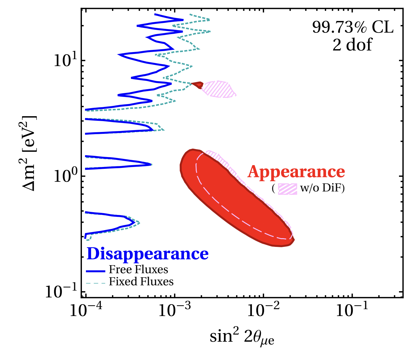
(a) From Ref. [11]

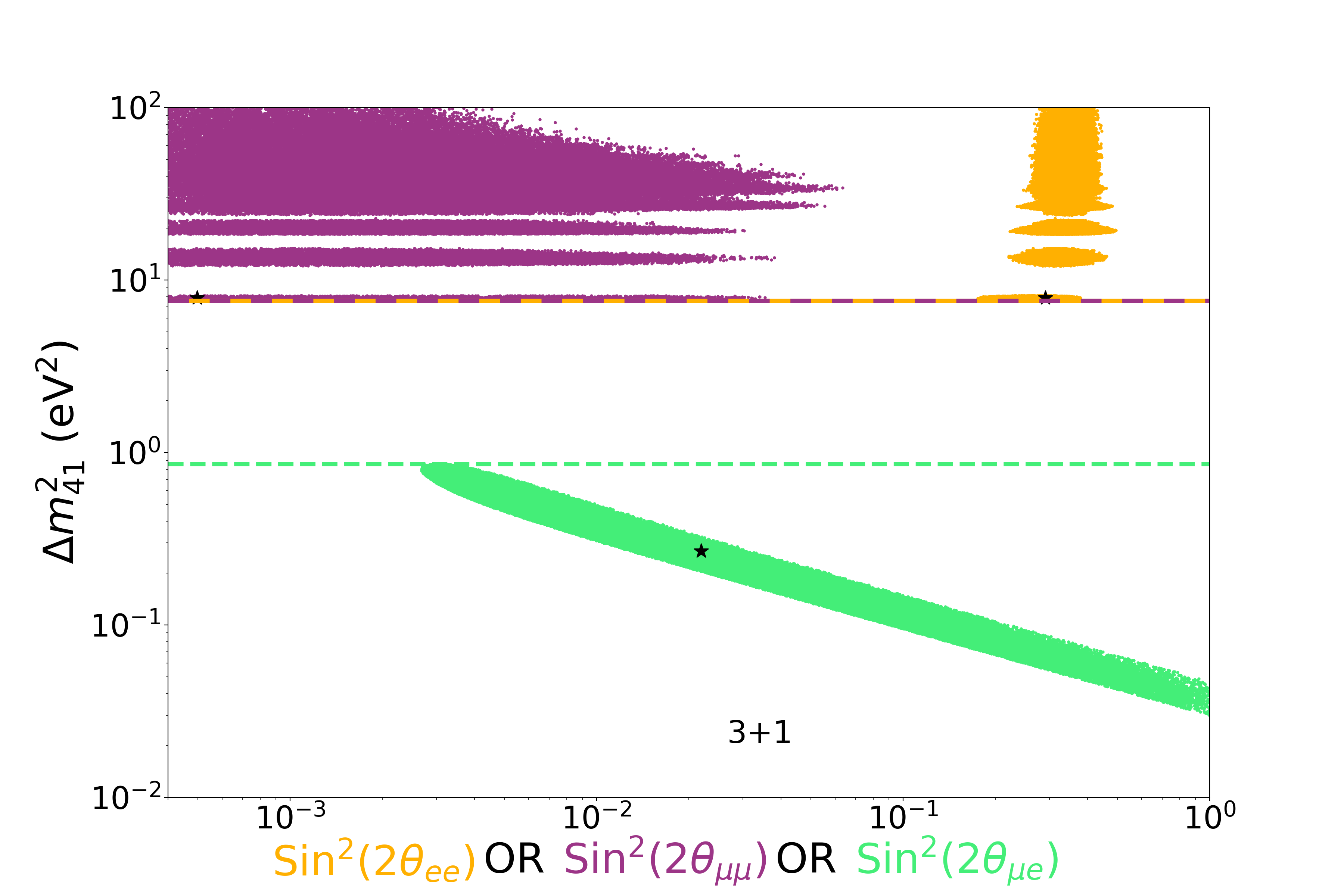
(b) From Ref. [12]

Figure 1.15: Graphical representation of the tension observed in 3+1 global fits between different subsets of the experimental landscape. Figure 1.15(a) shows the tension between $\nu_{e}$ appearance experiments and $\nu_{e}$/$\nu_{\mu}$ disappearance experiments observed in Ref. [11]. Figure 1.15(b) shows the tension between allowed regions from $\nu_{e}$ appearance (lower right), $\nu_{e}$ disappearance (upper right), and $\nu_{\mu}$ disappearance (upper left) experiments observed in Ref. [12], which includes the latest results from the BEST experiment.

Chapter 2 The MiniBooNE Experiment

This chapter is intended to give the reader an overview of the Mini Booster Neutrino Experiment (MiniBooNE), specifically concerning the excess of electron-like events observed by MiniBooNE in data taken between 2002–2019 at Fermilab’s Booster Neutrino Beam (BNB). The MiniBooNE excess is at the center of this thesis; the research presented here covers both experimental follow-up and theoretical interpretations of this anomaly. Thus, the remaining chapters require a thorough discussion of the MiniBooNE experiment and its most famous result.

2.1 Overview of MiniBooNE

MiniBooNE was originally designed as an experimental follow-up to the LSND excess of $\overline{\nu}_{e}$ events observed at the Los Alamos Meson Physics Facility (LAMPF) [5]. As described in section 1.4, the LAMPF flux comprised mostly of $\overline{\nu}_{\mu}$, which dominated over the $\overline{\nu}_{e}$ flux by three orders of magnitude [107]. Because of this, LSND was able to perform a low-background search for the IBD interaction $\overline{\nu}_{e}p\to e^{+}n$. An excess of IBD events was observed above the intrinsic $\overline{\nu}_{e}$ flux prediction from the beam dump source–this is known as the “LSND amonaly” [5].

The LSND anomaly has traditionally been interpreted as evidence for $\overline{\nu}_{\mu}\to\overline{\nu}_{e}$ oscillations at $\Delta m^{2}\approx 1\;{\rm eV}^{2}$. The LSND detector sat relatively close to the LAMPF nuclear target; the characteristic length-to-energy ratio in the experiment was $L/E\sim 30\;{\rm m}/30\;{\rm MeV}$. According to equation 1.32, in order to be sensitive to the oscillation-based interpretation of the LSND anomaly, one must maintain the same ratio $L/E$. This was the design strategy of the MiniBooNE experiment, which observed the interactions of neutrinos from the BNB with characteristic energy $E_{\nu}\sim 500\;{\rm MeV}$, at a baseline of $L\sim 500\;{\rm m}$ from the BNB beryllium target. The BNB produced mostly $\nu_{\mu}$ from pion decay-in-flight; thus, MiniBooNE searched for $\nu_{\mu}\to\nu_{e}$ oscillations in the BNB at $\Delta m^{2}\approx 1\;{\rm eV}^{2}$.

2.1.1 The Booster Neutrino Beam

The BNB, which is still operational, follows the typical design of a neutrino beamline [107]. Protons are accelerated in a synchrotron up to a momentum of 8.89 GeV, at which point they are kicked out of the synchrotron and interact within the Be target of the BNB, producing a cascade of secondary particles [14]. The charged mesons in this cascade are then focused using a toroidal magnetic field from an aluminum horn. By switching the direction of the current in the horn (and thus the direction of the magnetic field), one can choose whether to focus positively-charged mesons and de-focus negatively-charged mesons (“neutrino mode”), or vice-versa (“antineutrino mode”). After focusing, charged mesons pass through a concrete collimator and enter a 50-meter-long air-filled region where they decay to neutrinos. The neutrinos travel through another 474 meters of bedrock before reaching the MiniBooNE detector. A schematic depiction of this process is shown in figure 2.1.

The MiniBooNE flux is described in detail in Ref. [14]; we summarize the most important details here. In neutrino (antineutrino) mode, the flux is dominated by $\nu_{\mu}$ ($\overline{\nu}_{\mu}$) from $\pi^{+}$ ($\pi^{-}$) decay. Wrong-sign $\overline{\nu}_{\mu}$ ($\nu_{\mu}$), coming mostly from the decay of oppositely-charged pions, contribute at the 5% (15%) level. Two and three-body kaon decays also contribute to the $\nu_{\mu}$ and $\overline{\nu}_{\mu}$ flux at the few-percent level. The BNB also produces electron (anti)neutrinos, which represent $<1\%$ of the total flux in both neutrino and antineutrino mode. These come from two main sources: the decay of the secondary muon produced in the original charged pion decay, which is dominant for $E_{\nu}\lesssim 1\;{\rm GeV}$, and two-body kaon decay, which is dominant for $E_{\nu}\gtrsim 1\;{\rm GeV}$. The BNB flux breakdown in neutrino and antineutrino mode are shown in figure 2.2.

The $\pi^{\pm}$ production rate from p-Be interactions has been measured by the HARP [108] and BNL E910 [109] experiments. HARP took data at the BNB proton incident momentum (8.89 GeV/c) with a replica of the BNB beryllium target, while E910 took data at varying incident proton momenta above and below the nominal BNB value. These data were used to constrain a Sanford-Wang parameterization of the $\pi^{\pm}$ differential production cross section in the BNB [110]. The charged and neutral kaon production rates in p-Be were constrained by measurements from other experiments at proton momenta around 8.89 GeV/c; the Feynman scaling hypothesis was used to relate these measurements to the BNB proton momentum [14].

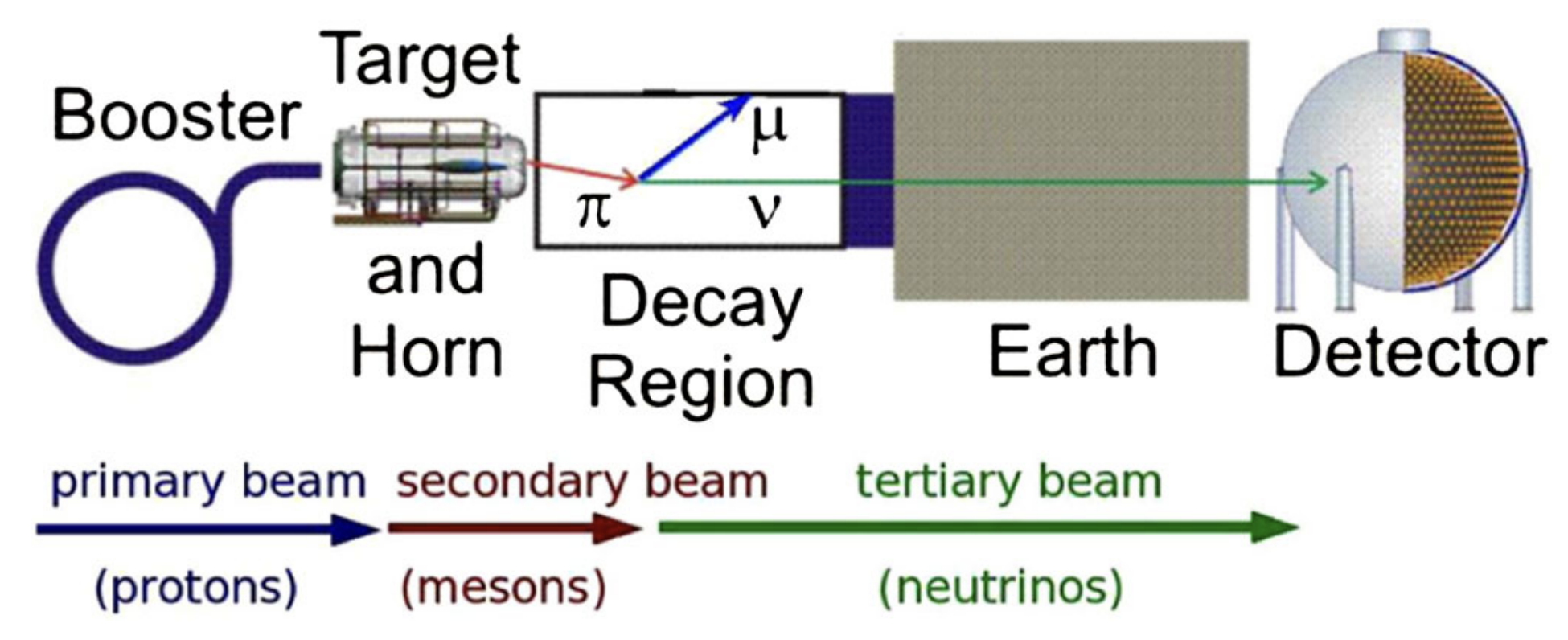
Figure 2.1: A schematic depiction of the BNB at Fermilab, including the downstream MiniBooNE detector. Figure from Ref. [13].

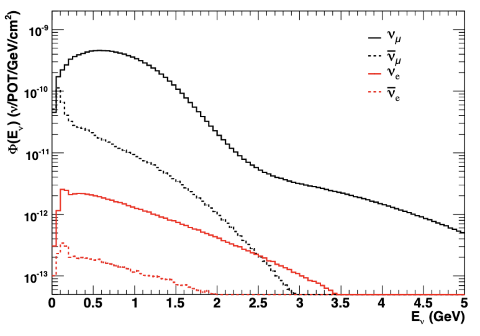
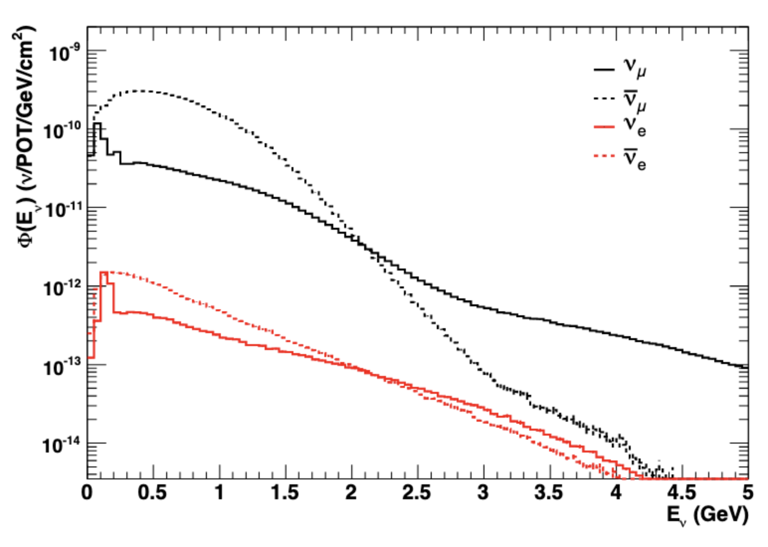
Figure 2.2: Breakdown of the neutrino flux at the BNB in neutrino (left) and antineutrino (right) mode. Figure from Ref. [14]

2.1.2 The MiniBooNE Detector

The MiniBooNE detector is an 818-ton, 6.1-meter-radius spherical volume filled with mineral oil (approximately CH₂) [15]. It was designed to measure the Cherenkov light produced from charged particles created in the charged-current interactions of BNB neutrinos within the detector volume. To do this, the inner surface of the sphere was instrumented with 1280 photo-multiplier tubes (PMTs), corresponding to a photocathode coverage of 11.3%. An additional 240 PMTs were used to instrument the surrounding veto region, which rejected cosmic muons and neutrino interactions outside the detector volume with an efficiency of $\sim 99.99\%$ [15]. Mineral oil was chosen as the detector medium due to its high index of refraction (n=1.47), leading to more Cherenkov light production by electrons traversing the detector volume. The exact mineral oil mixture, Marcol 7, was selected by optimizing the behavior of photons with wavelengths between 320 nm and 600 nm (e.g., requiring an extinction length greater than 20 m) [15]. The detector was situated in a cylindrical vault just below ground level, under $\sim 3\;{\rm m}$ of dirt. A schematic depiction of the MiniBooNE detector is shown in figure 2.3.

The reconstruction of the final state from a neutrino interaction in MiniBooNE relied on the detection of Cherenkov light. Specifically, the collaboration developed reconstruction algorithms that turned the spatiotemporal distribution of photon hits on the PMTs into kinematic information on each observable final state particle [77]. These algorithms used maximum likelihood estimators to estimate the starting location, direction, and energy of final state particles using the observed photon hits in each PMT, relying on the known transport properties of Cherenkov photons within the detector medium. Cherenkov photons are emitted when a charged particle travels faster than the speed of light in a medium, at an angle of $\cos\theta_{C}=1/n\beta$ with respect to the charged particle track. This results in a characteristic ring-like pattern on the detector wall. Such Cherenkov rings formed the basis of the MiniBooNE reconstruction algorithm.

There were two main classes for observable final state particles in MiniBooNE: muon-like ($\mu$-like) and electron-like ($e$-like). Each elicits a different Cherenkov ring pattern [77]. At MiniBooNE energies, muons are typically minimum-ionizing particles and thus would appear as a uniform ring in the PMT array. The ring would be filled in if the muon exits the detector volume before going below the Cherenkov threshold, and would be open otherwise. Electrons, on the other hand, undergo radiative processes as they travel, emitting photons via the Bremsstrahlung process, which then undergo pair-production to $e^{+}e^{-}$, which then emit more photons, and so on. This process is typically called an “electromagnetic (EM) shower”. The multiple constituent electrons and positrons in this EM shower would result in a distorted Cherenkov ring in the PMT array. Importantly, high energy photons also produced these distorted rings after undergoing an initial pair-production interaction; thus, electrons and photons were essentially indistinguishable in MiniBooNE and were both classified as $e$-like. Another relevant final-state particle in MiniBooNE was the neutral pion, which could be identified via two separate distorted Cherenkov rings via the $\pi^{0}\to\gamma\gamma$ decay. It is also important to note that $\pi^{0}$ events could be misclassified as $e$-like if one of the photons was not reconstructed, which could happen if one of the photons escaped the detector without pair producing or had energy below the detection threshold. A schematic diagram of the detector signature of muons, electrons, and neutral pions in MiniBooNE is shown in figure 2.4(a).

A separate likelihood was calculated for three different final state particle hypotheses: electron, muon, and neutron pion [77]. Ratios of these likelihoods were used to distinguish one particle from another in MiniBooNE. As an example, we show the separation of electron and muon events as characterized by the log-likelihood-ratio as a function of reconstructed neutrino energy in figure 2.4(b). This ratio was the main selection tool in selecting $e$-like events for MiniBooNE’s flagship search for $\nu_{\mu}\to\nu_{e}$ oscillations in the BNB.

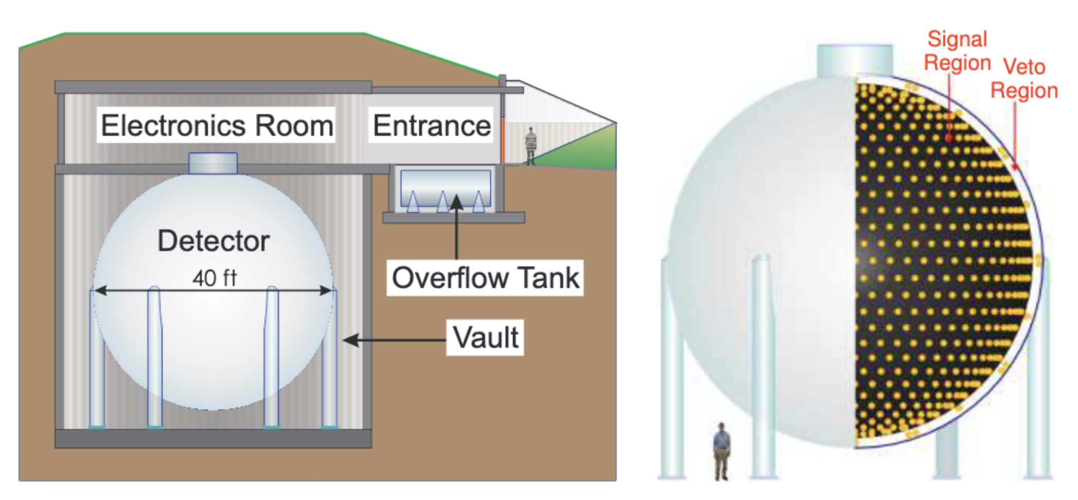
Figure 2.3: The MiniBooNE detector situated in the cylindrical detector hall (left) and an image of the interior of the MiniBooNE detector (right), showing the PMTs in both the signal and veto regions. Figure from Ref. [15].

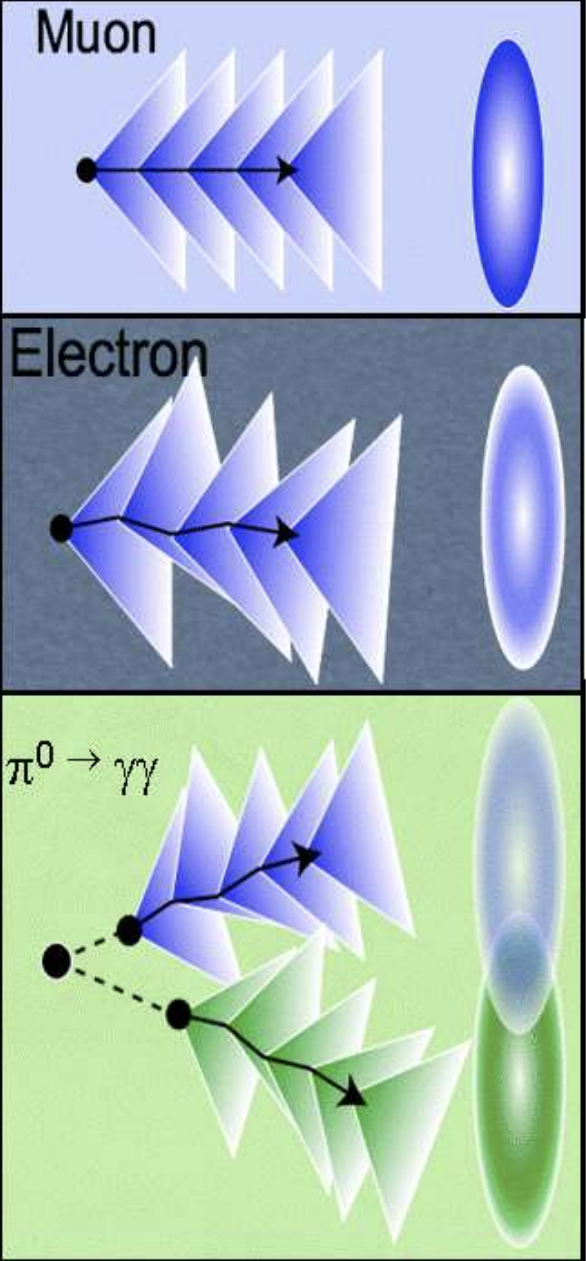
(a) From Ref. [76]

(b) From Ref. [77]

Figure 2.4: Visual representations of particle identification in MiniBooNE. Figure 2.4(a) shows a schematic representation of the detector signature from the three main particle classes in MiniBooNE: muons, electrons, and neutral pions. Figure 2.4(b) shows the MiniBooNE log-likelihood-ratio between the $e$-like and $\mu$-like hypothesis as a function of reconstructed neutrino energy, considering both simulated $\nu_{e}$ CCQE (top) and $\nu_{\mu}$ CCQE (bottom) interactions.

2.2 The MiniBooNE Low Energy Electron-Like Excess

As stated above, MiniBooNE was designed to test the LSND excess of $\overline{\nu}_{e}$ events discussed in section 1.4. To do this, MiniBooNE isolated a sample of $e$-like events using the likelihood ratios described in the previous section [76]. This sample was optimized to select $\nu_{e}$ CCQE interactions within the detector while rejecting $\nu_{\mu}$ interaction backgrounds, thus maximizing sensitivity to potential $\nu_{\mu}\to\nu_{e}$ oscillations within the BNB. MiniBooNE’s flagship $e$-like analysis, which has remained stable over the lifetime of the experiment, achieved a $\nu_{e}$ CCQE efficiency of $\sim 20\%$ while rejecting $\sim 99.9\%$ of $\nu_{\mu}$ backgrounds [10]. The full MiniBooNE dataset consists of $18.75\times 10^{20}$ ($11.27\times 10^{20}$) protons-on-target (POT) in neutrino (antineutrino) mode collected over 17 years of operation. In this dataset, the $e$-like analysis observes 2870 (478) data events in neutrino (antineutrino) mode, compared to an SM prediction of 2309.4 (400.6) events [10]. Combining neutrino and antineutrino mode data, MiniBooNE observes an excess of $638.0\pm 52.1\;({\rm stat.})\pm 122.2\;({\rm sys.})$ $e$-like events, corresponding to a Gaussian significance of $4.8\sigma$ [10].

Figure 2.5 shows the reconstructed neutrino energy distribution of the MiniBooNE $e$-like excess in both neutrino and antineutrino mode. The stacked histogram corresponds to the SM prediction from the NUANCE event generator [44], while the data points correspond to the observed number of $e$-like events in each bin. The error bars on the stacked histogram correspond to the systematic uncertainty on the SM prediction, calculated within a covariance matrix formalism. The dominant sources of systematic uncertainty include neutrino cross section modeling (derived largely using MiniBooNE’s own cross section measurements [111, 112, 113, 114]), nuclear effects, detector response and optical modeling, and BNB flux estimation [79, 10]. The presented error in each bin of the $\nu_{e}$ and $\overline{\nu}_{e}$ sample incorporates a constraint from MiniBooNE’s dedicated $\nu_{\mu}$ and $\overline{\nu}_{\mu}$ CCQE samples. The dashed line corresponds to the best fit of the MiniBooNE excess to the $3+1$ sterile neutrino model described in section 1.4. As one can see, the excess in data events is strongest in the lowest energy bins; for this reason, this anomaly is often referred to as the MiniBooNE low-energy excess (LEE).

As MiniBooNE used a Cherenkov detector, it was not sensitive to the final state hadronic activity in a neutrino interaction. Thus, kinematic reconstruction of the original neutrino relied entirely on the final state lepton. Under the assumption that the neutrino underwent a CCQE interaction off of a nucleon at rest within the nucleus, the original neutrino energy is given by [111]

$$E_{\nu}^{\rm QE}=\frac{2(M_{n}^{\prime})E_{\ell}-((M_{n}^{\prime})^{2}+m_{\ell}^{2}-M_{p})}{2[(M_{n}^{\prime})-E_{\ell}+\sqrt{E_{\ell}^{2}-m_{\ell}^{2}}\cos\theta_{\ell}]},$$ (2.1)

where $E_{\ell}$ is the total lepton energy, $\cos\theta_{\ell}$ is the lepton scattering angle, and $M_{n}$, $M_{p}$, and $m_{\ell}$ are the neutron, proton, and lepton mass, respectively. The adjusted neutron energy is defined as $M_{n}^{\prime}\equiv M_{n}-E_{B}$, where $E_{B}$ is the nuclear binding energy of the initial state neutron. An analogous relation exists for antineutrino energy reconstruction in a CCQE interaction [115]. This is the reconstructed energy definition used to generate the histograms in figure 2.5.

Figure 2.6 shows the visible energy and $\cos\theta$ distributions of the final state lepton in MiniBooNE’s $e$-like neutrino mode sample. The visible energy distribution shows the strongest discrepancy for softer lepton kinetic energies, as expected for a low-energy excess. For the angular distribution, it is worth noting that while there is an excess across the entire range, the largest deviation above the SM prediction comes from the $\cos\theta\in[0.9,1.0]$ bin. The angular distribution of the MiniBooNE LEE is an important piece of information for potential solutions to the anomaly–as we will discuss throughout this thesis, BSM physics models often cannot explain the energy and angular distributions of the MiniBooNE LEE simultaneously.

The green contributions to the stacked histograms of figure 2.5 represent the interactions of intrinsic $\nu_{e}$ or $\overline{\nu}_{e}$ in the BNB. At low energies, these events come mostly from the decay of the secondary muon in the $\pi^{+}\to\mu^{+}$ or $\pi^{-}\to\mu^{-}$ decay chain, while $\nu_{e}$ and $\overline{\nu}_{e}$ from kaon decays start to contribute more at higher energies [14].

The red and brown contributions to the stacked histograms represent misidentified photon backgrounds that are reconstructed as a single distorted Cherenkov ring. The largest photon background comes from misidentified $\pi^{0}$ created via $\nu_{\mu}$ and $\overline{\nu}_{\mu}$ neutral-current (NC) resonant scattering, in which the initial state nucleon is excited to a $\Delta$ resonance before decaying to nucleon-pion pair. The $\pi^{0}$ decay promptly to a pair of photons, which should nominally appear as a pair of distorted Cherenkov rings as in figure 2.4(a). However, if one of the photons exits the detector before converting to an $e^{+}e^{-}$ pair, or if the original pion energy is distributed asymmetrically such that the visible energy of one of the photons sits below the reconstruction threshold of 140 MeV [76], the $\pi^{0}$ decay will be misidentified as an $e$-like event. An enhancement of the NC $\pi^{0}$ background in figure 2.5 could in principle explain the observed excess. However, MiniBooNE constrained the rate of this NC $\pi^{0}$ background in situ via a measurement of the two-gamma invariant mass peak in well-reconstructed NC $\pi^{0}$ events [10]. Additionally, the radial distribution of the excess peaks toward the center of the detector, while misidentified NC $\pi^{0}$ backgrounds happen more often toward the edge of the detector, where it is more likely for a photon to escape before pair-producing.

The next-largest photon background comes from rare $\Delta\to N\gamma$ decays in $\nu_{\mu}$ and $\overline{\nu}_{\mu}$ NC resonant scattering interactions. As this process has never been observed directly, it was not possible for MiniBooNE to constrain the $\Delta\to N\gamma$ event rate in situ. It was instead constrained indirectly by the NC $\pi^{0}$ two-gamma invariant mass distribution [10]. A factor 3.18 enhancement in $\Delta\to N\gamma$ events could explain the MiniBooNE LEE; however, this hypothesis has since been disfavored by recent results from the MicroBooNE experiment [80]. The MicroBooNE experiment will be covered in more detail in chapters 3, 4 and 5.

MiniBooNE has also studied neutrino interactions outside the detector volume which result in a single photon entering the detector (the “dirt” backgrounds in figure 2.5). The timing distribution of the MiniBooNE $e$-like dataset suggests that the excess comes primarily in time with the beam, while dirt background events are often delayed by $\sim 10\;{\rm ns}$ [10]. This result disfavors an enhancement of external neutrino interactions as an explanation of the MiniBooNE excess.

Therefore, the $4.8\sigma$ MiniBooNE excess remains unexplained. Resolution of the MiniBooNE LEE is one of the major goals of the neutrino community [83].

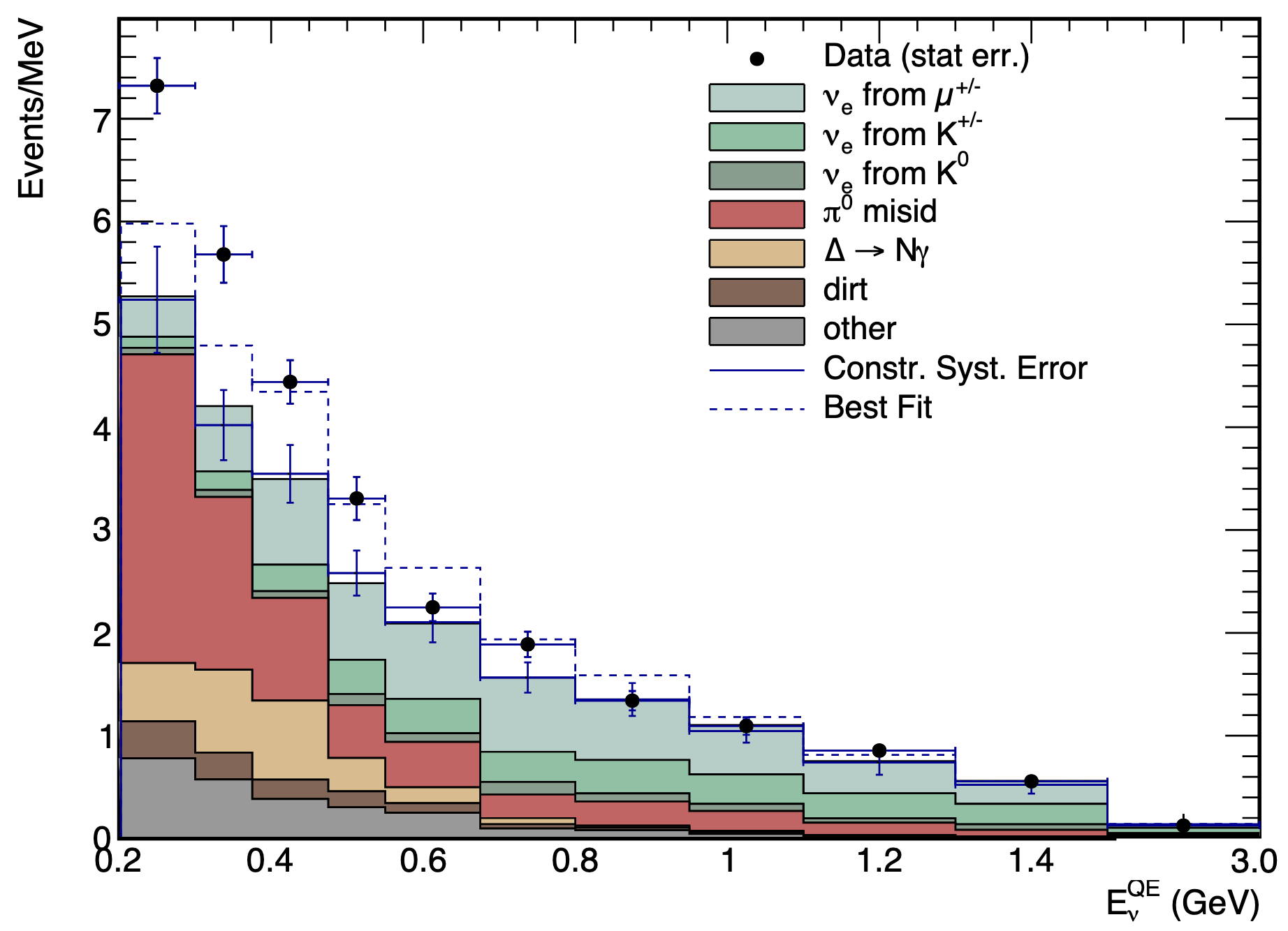
(a) $\nu_{e}$ sample, from Ref. [10]

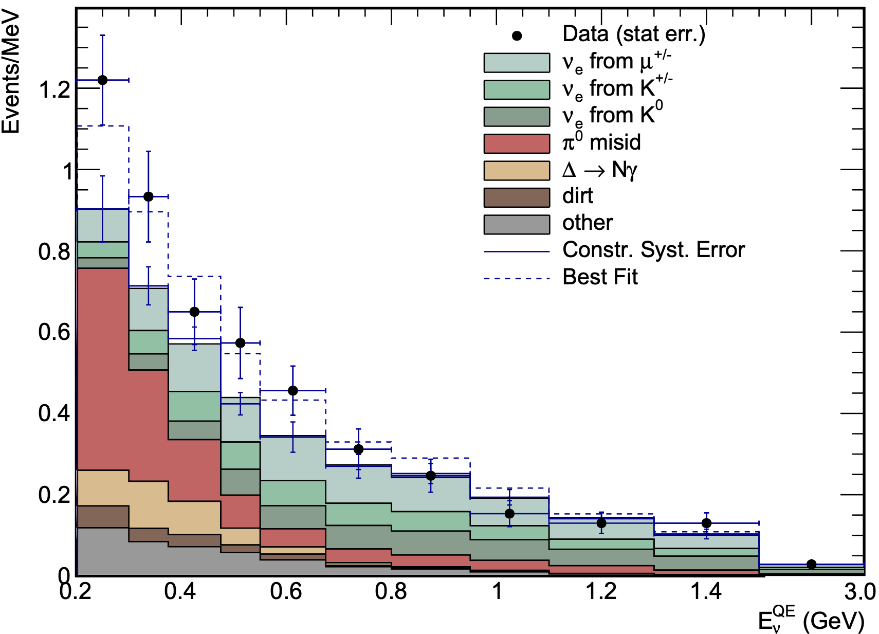
(b) $\overline{\nu}_{e}$ sample, from Ref. [79]

Figure 2.5: The $E_{\nu}^{\rm QE}$ distribution of the MiniBooNE $e$-like excess in the total neutrino mode (figure 2.5(a)) and antineutrino mode (figure 2.5(b)) datasets. The observation and SM prediction in each bin are shown by the data points and colored histograms, respectively.

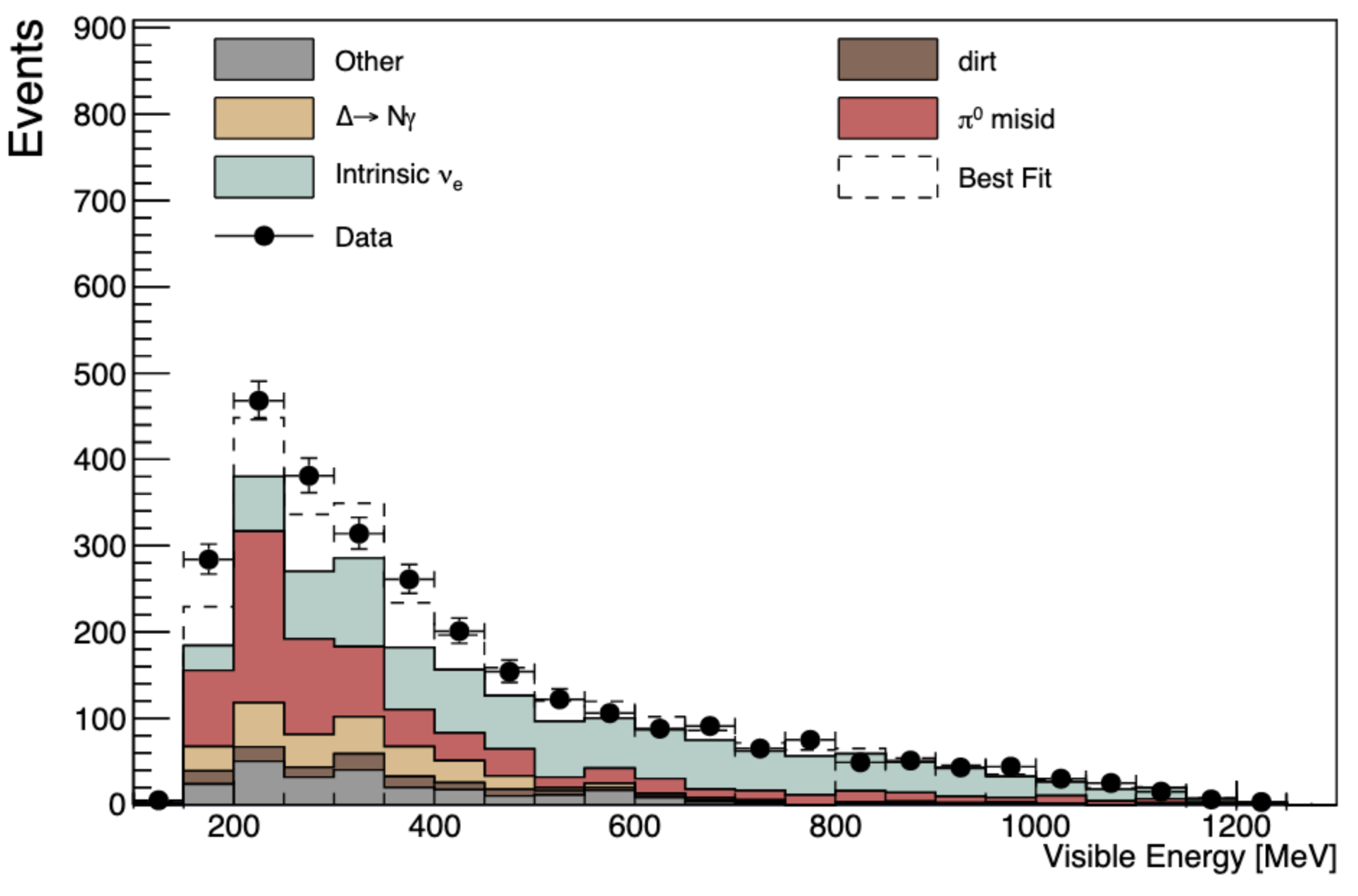
(a) Lepton $E_{\rm vis}$ distribution

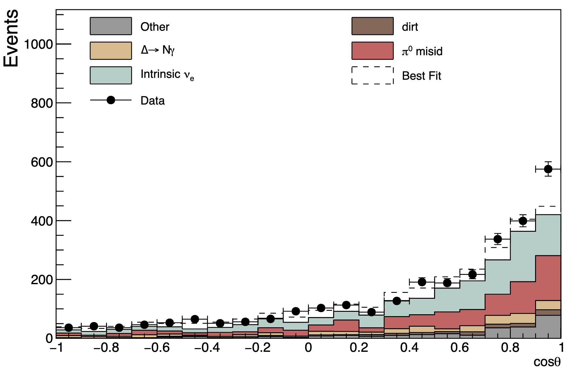
(b) Lepton $\cos\theta$ distribution

Figure 2.6: The lepton visible energy (figure 2.6(a)) and $\cos\theta$ (figure 2.6(b)) distributions of the MiniBooNE $e$-like excess in the total neutrino mode dataset. The observation and SM prediction in each bin are shown by the data points and colored histograms, respectively. Figures from Ref. [10].

The MiniBooNE LEE is most commonly interpreted within the context of the 3+1 model introduced in section 1.4. This is primarily because the MiniBooNE excess has historically been considered alongside the LSND excess, as both results can be explained by short-baseline $\nu_{\mu}\to\nu_{e}$ and $\overline{\nu}_{\mu}\to\overline{\nu}_{e}$ appearance. Strikingly, the MiniBooNE and LSND anomalies both prefer similar regions in sterile neutrino parameter space, as shown in figure 1.14. This is further supported by figure 2.7, which shows the rising nature of the MiniBooNE and LSND excesses as a function of the ratio $L/E$, behavior that is consistent with a sterile neutrino explanation.

There are, however, complications regarding a sterile neutrino explanation of the MiniBooNE excess. The 3+1 model has difficulty reproducing the lowest energy and lowest scattering angle region of the excess. Figure 2.6 shows that the best fit 3+1 prediction, indicated by the dotted line, still falls below the observed data in the lowest lepton $E_{\rm vis}$ bin and highest lepton $\cos\theta$ bin. Additionally, as discussed in section 1.4, there is significant tension between the MiniBooNE and LSND observation of $\nu_{e}$/$\overline{\nu}_{e}$ appearance and experiments searching for $\nu_{e}$/$\overline{\nu}_{e}$ and $\nu_{\mu}$/$\overline{\nu}_{\mu}$ disappearance. Finally, the follow-up MicroBooNE experiment has not observed an excess of $\nu_{e}$ events consistent with the expectation from the MiniBooNE LEE [116]. The MicroBooNE $\nu_{e}$ analysis is one of the main results of this thesis and will be explored in more detail in chapters 4 and 5. While the non-observation of a MiniBooNE-like excess of $\nu_{e}$ events in the BNB does set constraints on $3+1$ parameter space, it does not fully exclude the MiniBooNE allowed regions [102]. This point will be discussed further in chapter 5.

These complications with the eV-scale sterile neutrino interpretation of the MiniBooNE LEE have prompted the community to explore alternative explanations. Many of these are relatively simple extensions beyond $3+1$, such as $3+N$ models involving $N$ additional sterile neutrino states [93], decaying sterile neutrino models [117, 118, 119], and sterile neutrinos with altered dispersion relations from large extra dimensions [120, 121, 122]. Other explanations for the MiniBooNE LEE introduce a number of new particle species prescribed with new interactions that create an additional source of photons or $e^{+}e^{-}$ pairs in MiniBooNE. Such models include heavy neutral leptons (HNLs) which decay to photons via a transition magnetic moment [123, 124, 125, 126, 127, 128, 129, 130, 131, 132, 133, 134, 27, 135, 31] and models with heavy neutrinos coupled to a “dark sector” involving, for example, new vector or scalar mediators [136, 137, 138, 139, 140, 141, 142, 143, 144, 145, 146]. Chapter 6 of this thesis explores one such explanation of MiniBooNE involving an HNL with a transition magnetic moment coupling to active neutrinos, which we hereby refer to as a “neutrissimo”. Neutrissimo decays in MiniBooNE provide an additional source of single photons which could explain the $e$-like excess [27, 31].

Thus, there are many potential explanations for the MiniBooNE anomaly. Distinguishing between these explanations requires careful consideration of the kinematic distributions of the MiniBooNE excess [147, 31]. Further, these models are often subject to constraints from existing accelerator neutrino experiments, such as MINERvA and NA62 [146, 139]. A complete evaluation of constraints from existing data is essential in determining the most viable models among the many proposed MiniBooNE explanations. The work presented in chapter 6 takes a step in this direction by calculating constraints from MINERvA on the neutrissimo model.

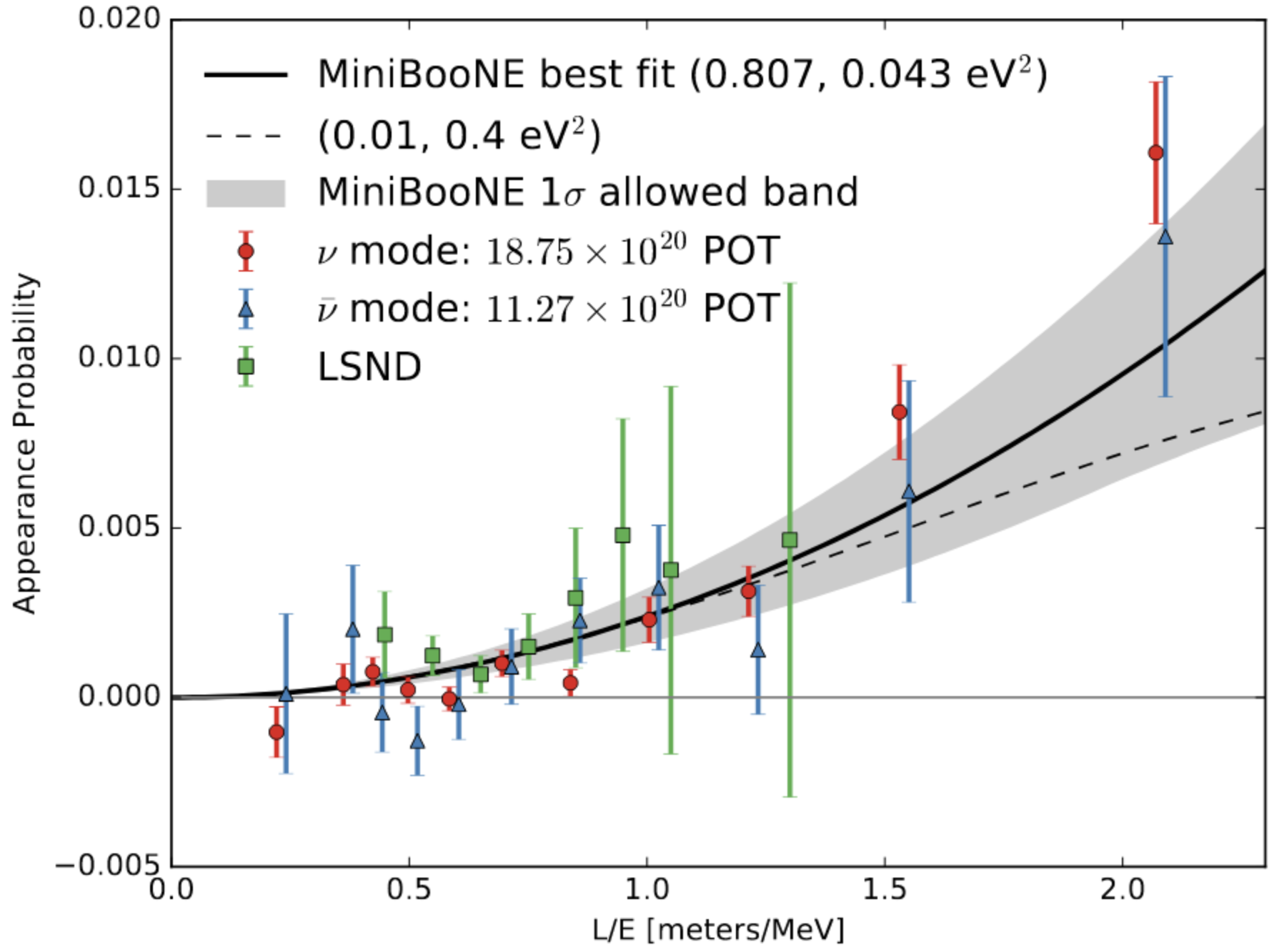
Figure 2.7: The MiniBooNE and LSND excesses as a function of the ratio $L/E$. The MiniBooNE data is separated into neutrino and antineutrino mode. Figure from Ref. [10].

Chapter 3 The MicroBooNE Detector

In order to ascertain the nature of the MiniBooNE excess, one needs a detector capable of providing more detailed event-by-event information than MiniBooNE’s Cherenkov detector. This is the concept behind the MicroBooNE experiment. The MicroBooNE detector is a large-scale liquid argon time projection chamber (LArTPC) with the ability to record high-resolution images of neutrino interactions. MicroBooNE recently released its first results investigating the nature of the MiniBooNE excess [116, 80], which will be presented in chapters 4 and 5. This chapter introduces the detector that made this measurement possible.

3.1 Liquid Argon Time Projection Chamber

MicroBooNE used an 85-metric-ton fiducial volume LArTPC detector to observe the interactions of neutrinos in the BNB [16, 148]. This makes MicroBooNE the first $\mathcal{O}(100~{}{\rm t})$ LArTPC operated in the United States. The idea for a LAr-based total absorption detector originated in the 1970s [149]. The introduction of the LArTPC detector concept came from Carlo Rubbia in 1977 [150], extending earlier work from David Nygren [151] and Georges Charpak [152]. The first operational large-scale LArTPC was the 500-metric-ton active volume ICARUS T600 detector [153], which came online in 2010. ICARUS observed cosmic ray and neutrino interactions at the Gran Sasso underground National Laboratory [154] and even set constraints on $\nu_{\mu}\to\nu_{e}$ interpretations of the LSND and MiniBooNE anomalies using the CERN to Gran Sasso neutrino beam [155]. On a smaller scale, the ArgoNeuT experiment operated a 0.25-metric-ton LArTPC at Fermilab’s Neutrino Main Injector beamline from 2009-2010, where it performed the first measurements of neutrino-argon cross sections [156].

The MicroBooNE detector is situated $70$ m downstream of the MiniBooNE detector along the BNB and operated from 2015 to 2021, observing a total of approximately $1.5\times 10^{21}$ POT [148]. MicroBooNE LArTPC data come in the form of high-resolution three-dimensional images of the ionization energy deposited by final state charged particles in neutrino interactions. The information contained in these images allows for the event-by-event separation of photons and electrons–an essential capability for determining the source of the MiniBooNE excess. MicroBooNE can also reconstruct hadronic activity in the final state of the neutrino interaction, which helps further distinguish between the possible sources of the MiniBooNE excess.

We begin with a brief overview of the MicroBooNE reconstruction procedure. Charged-current neutrino interactions in the LAr volume produce charged particles in the final state, which ionize argon atoms as they traverse the detector. Thus, each charged particle leaves behind a trail of ionized electrons which, in theory, can drift freely through the noble element detector medium without being captured. This drift is controlled via an external electric field with strength $|E|\sim 273$ V/cm, accelerating the ionized electrons to a final velocity $v\sim 0.11$ cm/$\mu$s toward three anode wire planes [148]. MicroBooNE employs a right-handed coordinate system, in which BNB neutrinos travel along the $\hat{z}$ direction, ionization electrons drift along the $-\hat{x}$ direction, and $\hat{y}$ represents the vertical direction [16]. The anode planes consist of two induction planes and one collection plane, each containing a series of wires spaced 3 mm apart and oriented at $\pm 60^{\circ}$ and $0^{\circ}$ with respect to the $\hat{y}$ direction for the induction and collection planes, respectively. Each plane is biased such that ionization electrons drift past the induction plane wires, generating a signal via induction, and terminate on the collection plane wires, generating a signal via direct charge collection. The signals on the anode wire planes allow for two-dimensional reconstruction of the charged particle trajectory in the $\hat{y}-\hat{z}$ plane, transverse to the drift direction. The $\hat{x}$ dimension of the charged particle trajectory can be reconstructed using the arrival time of signals on the anode wires in conjunction with the known drift time of the ionization electrons. In order for this technique to work, one must know the initial time at which the charged particle entered the detector. This can be established using either an external beam trigger or an internal trigger from the light collection system, which operates on much shorter time scales, $\mathcal{O}({\rm ns})$, compared to characteristic electron drift times of $\mathcal{O}({\rm ms})$. A schematic of this process is shown in figure 3.1.

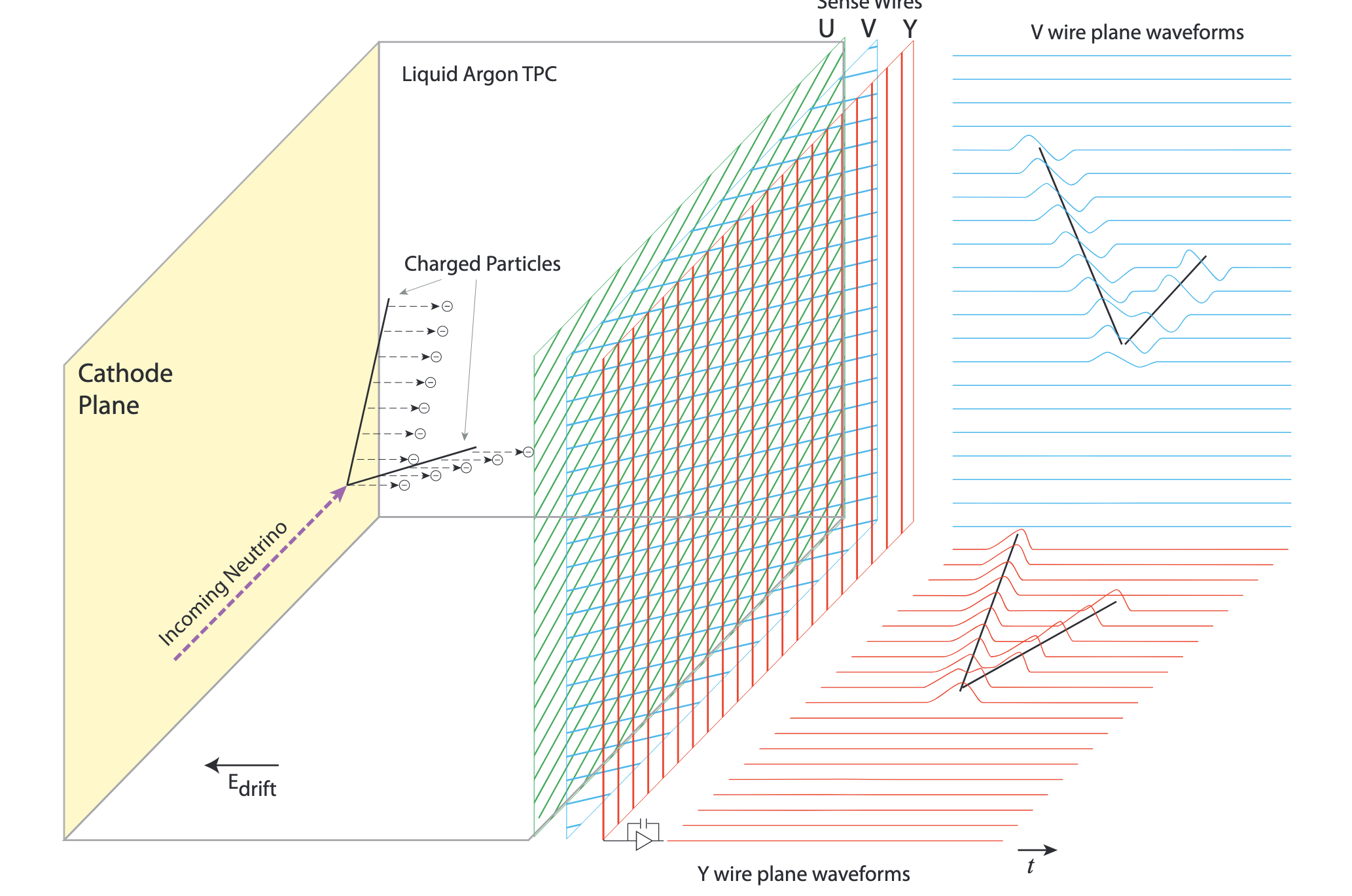
(a)

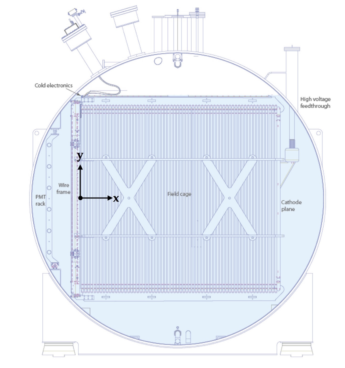
(b)

Figure 3.1: Schematic depictions of the MicroBooNE LArTPC. Figure 3.1(a) shows the detection process for charged particles from a neutrino interaction in a MicroBooNE-like LArTPC. Figure 3.1(b) shows a cross-sectional view of the MicroBooNE detector along the $-\hat{z}$ direction. Figures from Ref. [16].

3.1.1 Cryogenics

The MicroBooNE detector is relatively large–the LArTPC volume spans 2.6 m, 2.3 m, and 10.4 m in the $\hat{x}$, $\hat{y}$, and $\hat{z}$ direction, respectively [16]. Thus, ionization electrons must drift through $\mathcal{O}(m)$ of LAr before reaching the anode wire planes. Reconstruction of these ionization electrons requires careful control of the drift process. This is the main objective of the MicroBooNE cryogenic system.

The LArTPC is housed within a larger cylindrical cryostat, which itself is supported by an argon purification system and nitrogen refrigeration system [16]. The purification system consists of two recirculation pumps and two filter skids that remove electronegative impurities from the LAr, mainly oxygen (O₂) and water (H₂O). These impurities must be kept below the 100 parts-per-trillion O₂-equivalent level in order to maintain electron drift lengths of at least 2.5 m [157, 16]. Additionally, the nitrogen contamination must be kept below 2 parts-per-million in order to maintain an argon scintillation light attenuation length greater than the size of the detector [158]. Nitrogen cannot be appreciably removed from the argon via the purification system; rather, the initial nitrogen contamination is fixed by the quality of the delivered argon, and additional contamination must be controlled by minimizing the atmosphere leakage rate into the cryostat.

The nitrogen refrigeration system is designed to combat the heat load on the LAr from the environment and electrical power systems, maintaining thermal homogeneity throughout the active volume. It consists of two condensers, each designed to handle a heat load of approximately 9.5 kW [16]. The temperature of the LAr volume must be stable to $\pm 0.1$ K in order to keep the $\hat{x}$ direction resolution of charged particle tracks below 0.1% [16].

3.1.2 LArTPC Drift System

The drift system inside the LArTPC volume consists of three major subsystems: the cathode plane, the field cage, and the three anode wire planes. The purpose of the drift system is to maintain a uniform electric field throughout the active volume such that ionization electrons are transported to the anode plane at a stable drift velocity.

The cathode consists of nine stainless steel sheets connected to a supporting frame to form a single plane. Laser tracker measurements indicate that a majority of the cathode plan is flat to within $\pm 3$ mm [16]. The cathode plane is kept at a negative potential of approximately $-70$ kV via a high voltage feedthrough on the cryostat. The field cage maintains a uniform electric field between the cathode plane and anode planes. It consists of 64 stainless steel tubes wrapped around the LArTPC active volume. A resistor divider chain connects each tube to its neighbor, sequentially stepping the voltage from $-70$ kV to ground in $1.1$ kV increments. The chain provides a resistance of 250 M$\Omega$ between adjacent tubes such that the current flow is approximately 4.4 $\mu$A, much larger than the $\mathcal{O}({\rm nA})$ current from signals on anode plane wires [16]. Figure 3.2 shows the MicroBooNE cathode and field cage, as well as a simulated map of the electric field within the LArTPC active volume.

Perhaps the most critical components of the MicroBooNE detector are the three anode wire planes. The U and V induction planes contain 2400 wires each, while the Y collection plane contains 3456 wires. As mentioned above, the U and V plane wires are oriented at $\pm 60^{\circ}$ with respect to the vertical, while the Y plane is oriented vertically. The U, V, and Y planes are biased at -200 V, 0 V, and +440 V, respectively, to ensure termination of ionization electrons on the Y collection plane. Each wire is 150 $\mu$m in diameter and is spaced 3 mm from its neighbors. The planes themselves are spaced 3 mm from one another. The wires are held in place by wire carrier boards, which house 16 wires each in the U and V planes and 32 wires in the Y plane. Each wire is terminated using a semi-automated wrapping procedure around a 3 mm diameter brass ferrule. On the wire carrier boards, each wire makes contact with a gold pin that connects to the electronic read-out system. The anode planes are held in place by a single stainless steel frame, which houses each wire carrier board via an array of precision alignment pins. Wires are tested to withstand three times the nominal load of 0.7 kg without breakage, both before and after placement onto the wire carrier board. Figure 3.3(a) shows an image of a single Y plane wire carrier board with 32 mounted wires. An image of the fully-assembled MicroBooNE LArTPC is shown in figure 3.3(b), specifically highlighting the anode planes mounted on the stainless steel frame.

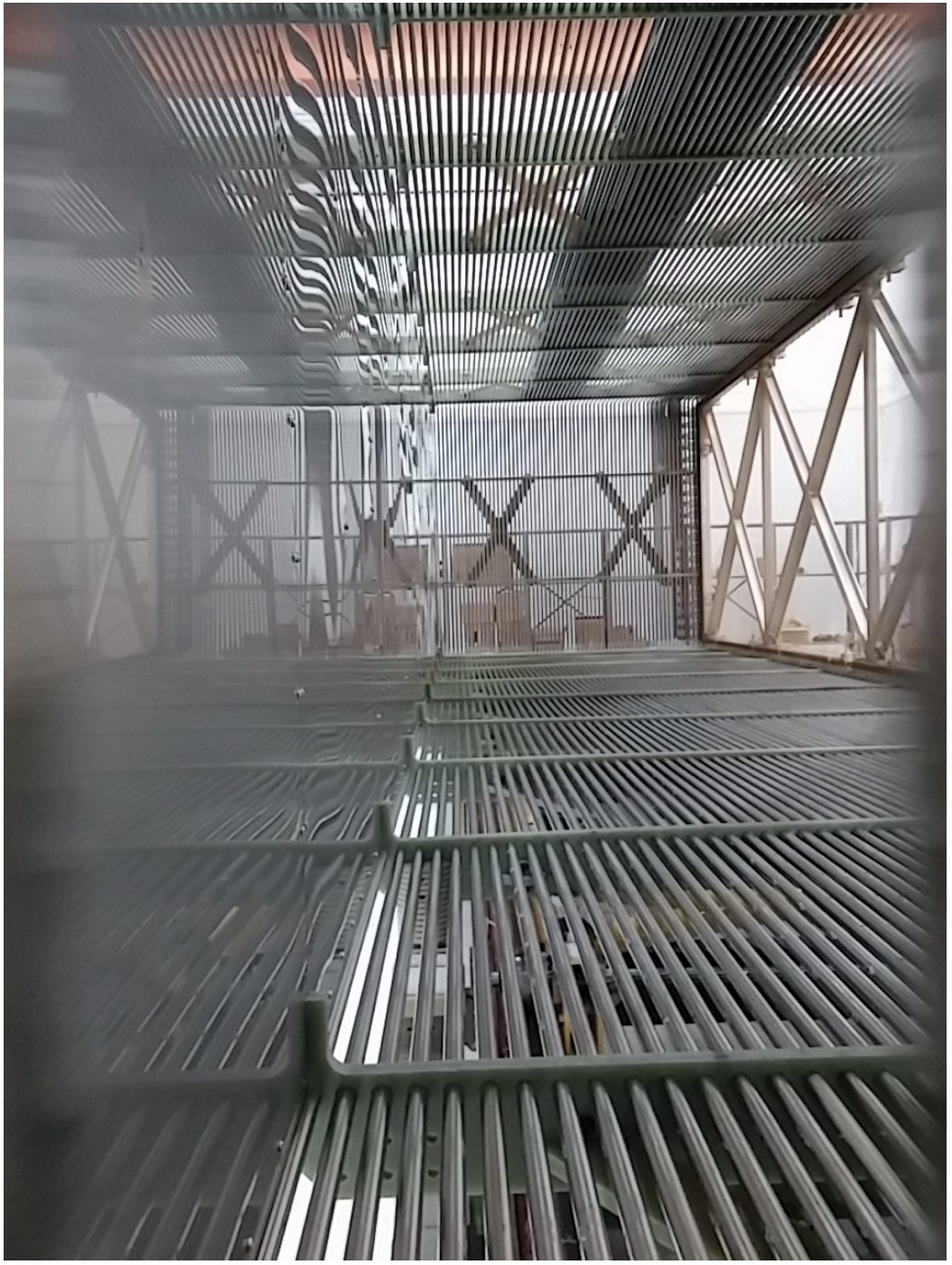
(a)

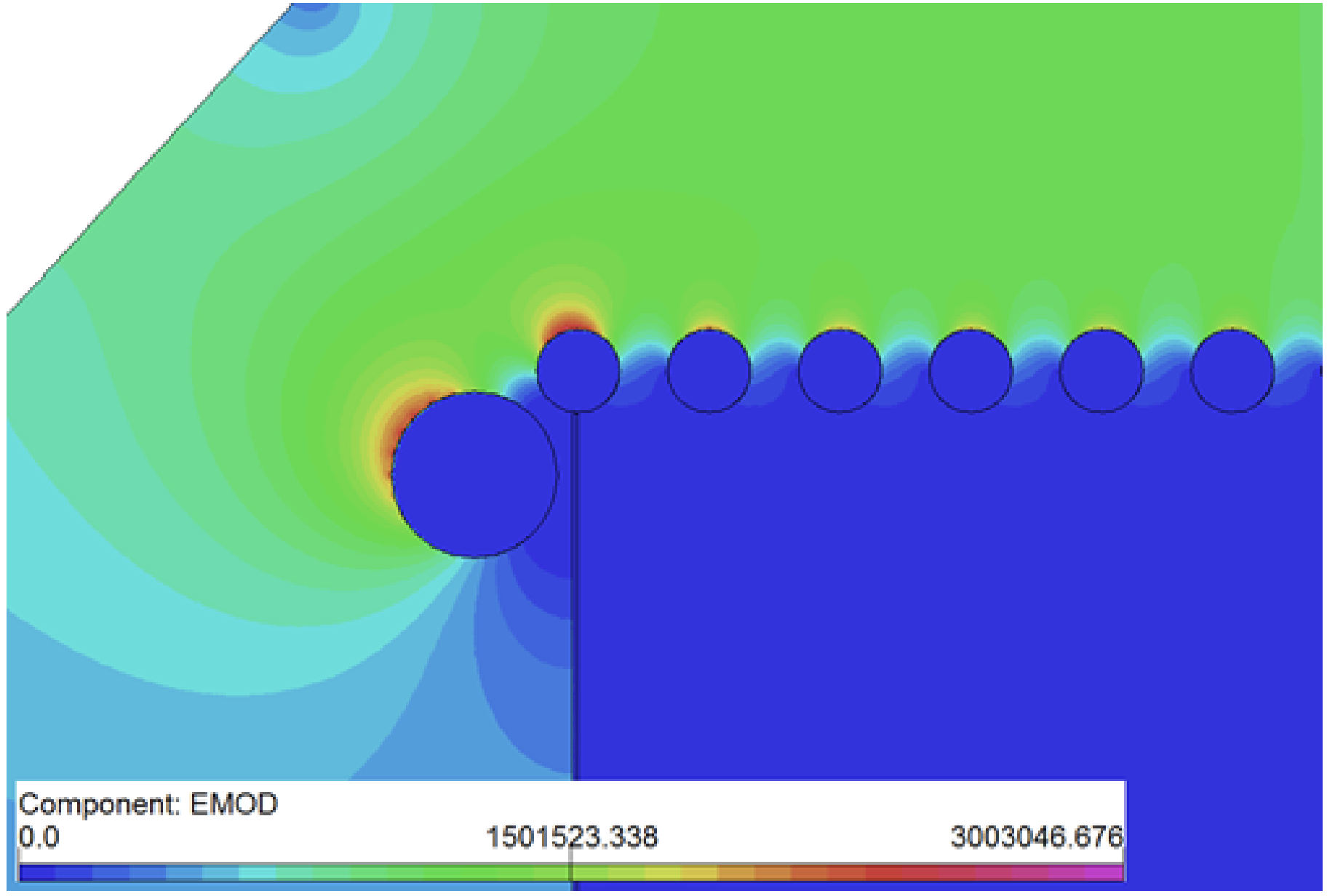
(b)

Figure 3.2: Figure 3.2(a) shows a close-up image of the cathode plane of the MicroBooNE LArTPC. The stainless steel field cage tubes can also be seen surrounding the active volume. Figure 3.2(b) shows a cross-sectional map of the electric field at the edge of the active volume, considering a cathode plane voltage of -128 kV. The legend shows the field strength in units of V/m. Figures from Ref. [16].

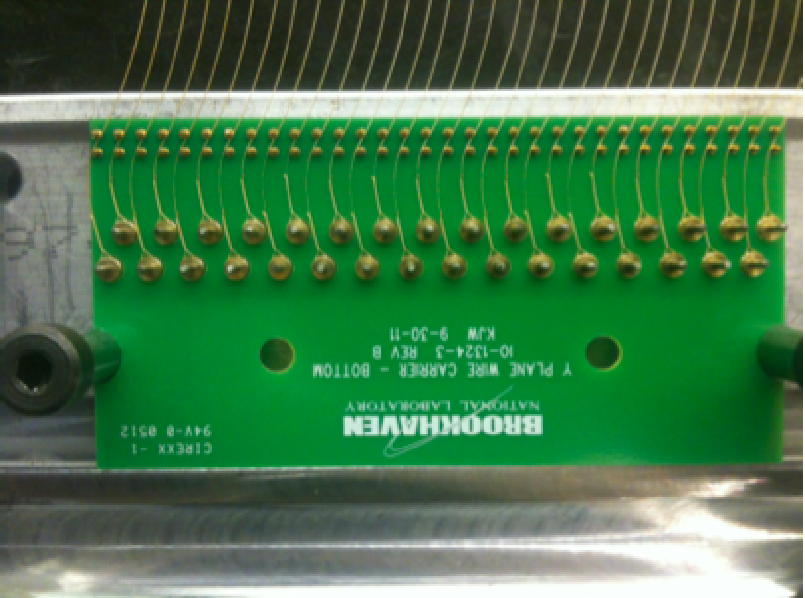
(a)

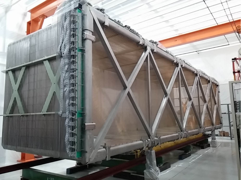
(b)

Figure 3.3: Figure 3.3(a) shows a photograph of a single wire carrier board with 32 mounted wires. Figure 3.3(b) shows the fully-assembled MicroBooNE LarTPC, highlighting the anode plane mounted on the stainless steel frame. Figures from Ref. [16].

3.1.3 Light Collection System

Liquid argon is a prolific scintillation medium due to its low cost, high scintillation yield ($\mathcal{O}(10^{4})$ photons per MeV of deposited energy), and transparency to its own scintillation light [158]. This last feature comes from the scintillation mechanism in LAr: when argon atoms are ionized, they combine with one another to form singlet and triplet excimer states. When these excimer states decay, they emit 128 nm photons which pass unattenuated through the surrounding atomic argon [159]. The decay of the singlet (triplet) state happens on timescales of $\mathcal{O}$(ns) ($\mathcal{O}$($\mu$s)) [160, 161]. Thus, scintillation light emission happens on much shorter timescales than the $\mathcal{O}$(ms) drift time of the ionization electrons.

The light collection system in MicroBooNE is designed to detect the scintillation photons produced in a neutrino interaction. It consists of 32 8-inch Hammamatsu R5912-02mod cryogenic PMTs situated behind an acrylic plate coated with tetraphenyl butadiene (TPB) [16]. An image of one such PMT assembly is shown in figure 3.5(a). TPB is a wavelength shifter that absorbs the 128 nm argon scintillation light and re-emits a photon in the visible range. The necessity of this procedure is shown in figure 3.4, which demonstrates that, unlike direct LAr scintillation light, TPB emission is well within the wavelength acceptance range of the PMTs.

When a photon hits the bi-alkali photocathode surface of an R5912-02mod PMT, an electron is released via the photoelectric effect [162]–this electron is often referred to as a “photoelectron” (p.e.). Each p.e. is focused toward a dynode chain–a series of electrodes designed to produce a number $n>1$ electrons for each incident electron, resulting in an avalanche of electrons by the final anode which can be read out in the form of a current. The wavelength-dependent probability with which a given p.e. enters the dynode chain is known as the “quantum efficiency“ of the PMT. At the nominal operating temperature of 87 K, the MicroBooNE PMTs have an average quantum efficiency of 15.3% [16]. Each PMT was tested in a liquid nitrogen (77 K) cryogenic environment, in which the gain and rate of thermal emission (“dark current”) of the PMT were measured as a function of the supplied high voltage (HV) across the dynode chain [163]. The HV for each PMT was set to produce a gain of $3\times 10^{7}$ at 77 K [16], corresponding to a dark current of $\mathcal{O}$(kHz) [163]. The current output from each PMT passed through preamp/shaper boards before being digitized via an analog-to-digital converter (ADC) with a sampling rate of 64 MHz [16]. Thus, light is collected in time ticks with a length of 15.625 ns [148].

The light collection system was critical in detecting activity in the detector coincident with a beam spill, indicating the presence of a neutrino interaction. In order to record a given event, at least 5 photoelectrons must have been detected across all PMTs [148]. Additionally, a “common optical filter” was applied to reduce the non-neutrino trigger rate–this filter required at least one string of six time ticks with greater than 20 photoelectrons detected during the 1.6 $\mu$s beam spill window, and no such strings of six time ticks in the 2 $\mu$s prior to the beam spill. The spatiotemporal distribution of light observed by the PMTs can also be used to augment the signal from the wire planes. For example, the PMT signal from a cosmic muon which stops in the detector and decays to a Michel electron is shown in figure 3.5(b).

The scintillation light yield and detection efficiency in liquid argon are impacted by a number of phenomena. Impurities can dissociate the argon excimers before they have a chance to emit scintillation light. For example, O₂ molecules in the LAr volume can undergo a two-body collision with an argon excimer [164],

$${\rm Ar}_{2}^{*}+{\rm O}_{2}\to 2{\rm Ar}+{\rm O}_{2}.$$ (3.1)

This interaction mainly decreases the decay probability of the longer-lived triplet state. Because of this, measurements of the delayed scintillation lifetime in LAr are sensitive to the concentration of impurities in the detector [160, 164, 16].

Scintillation light can also be absorbed by impurities within the detector. At concentrations of around 2 ppm, dissolved nitrogen will decrease the attenuation length of 128 nm scintillation light to around 30 m [165, 158]. TPB emanation from the painted acrylic plates can also lead to a bulk fluorescence effect within the liquid argon [166]. Additionally, Rayleigh scattering can deflect scintillation photons, diminishing the detector’s capability to translate photon detection into spatial information regarding the path of the original charged particle. The Rayleigh scattering length for 128 nm photons in liquid argon has been measured to be approximately 55 cm [167]. Given the size of the MicroBooNE detector, scintillation photons will undergo around five Rayleigh scattering interactions on average before reaching a PMT.

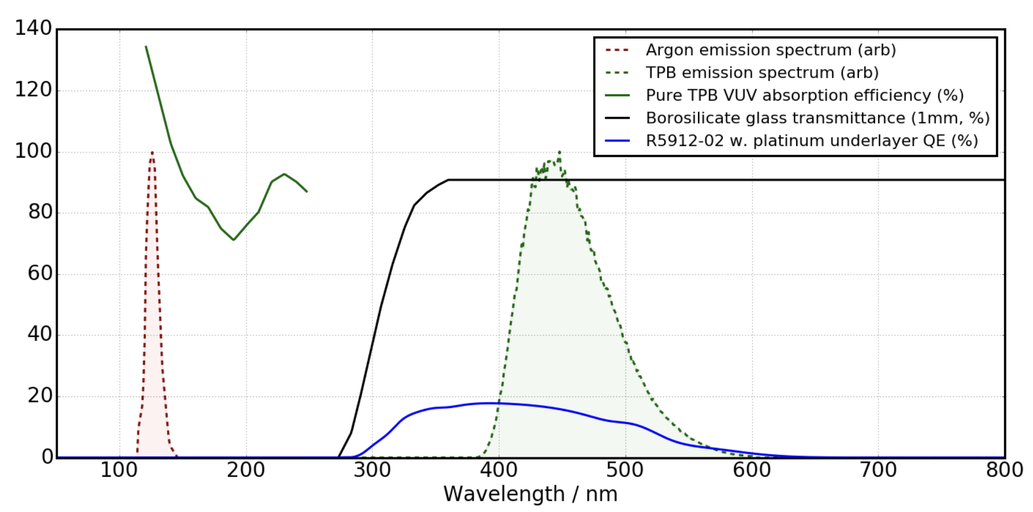
Figure 3.4: The LAr scintillation light spectrum, TPB ultra-violet absorption spectrum, TPB emission spectrum, PMT quantum efficiency, and PMT surface transmission efficiency as a function of photon wavelength. Figure from Ref. [17].

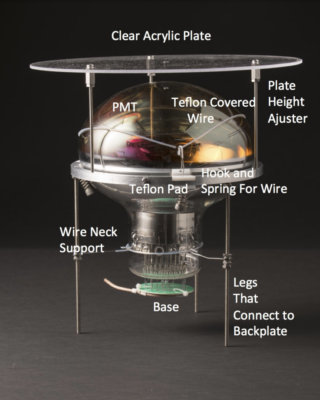
(a)

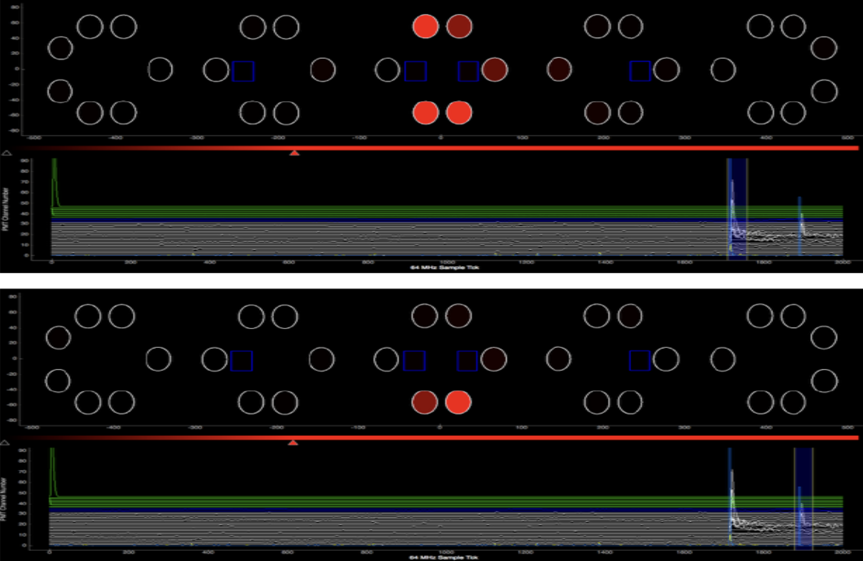
(b)

Figure 3.5: Figure 3.5(a) shows a photograph of a single PMT system used in the MicroBooNE detector. The acrylic window here has not yet been coated with TPB. Figure 3.5(b) shows the PMT signal from a stopped cosmic muon (top) that decays to a Michel (bottom). Figures from Ref. [16].

3.2 TPC Signal Processing

MicroBooNE has developed a custom cryogenic electronics system to amplify and digitize the analog signal on each wire of the LArTPC [16]. The wire signals first pass through front-end ASICs located on cryogenic motherboards attached directly to the wire carrier boards on the LArTPC. Each ASIC amplifies and shapes the signal from 16 wires–thus, 516 ASICs are needed to fully instrument the 8,256 readout channels of the LArTPC. Cryogenic-tested cables carry signals from the ASICs to intermediate amplifiers directly outside the cryostat, after which the signals travel through 20 m cables to the readout system. This system consists of 130 readout modules, each containing 8 custom-designed 12-bit ADCs and a Front End Module (FEM). Each ADC digitizes the signal from 8 wires at a rate of 16 MHz. The dynamic range of the ADC is set to enable the detection both of a minimum-ionizing particle far away from the anode planes and of a highly-ionizing-particle close to the anode planes without saturation. The FEM uses a field-programmable gate array (FPGA) to store and compress the digitized signals. Once a trigger is received, the FPGA sends 4.8 ms of TPC data to the data acquisition (DAQ) system. The 4.8 ms window is digitized into 9600 time ticks on each wire, with each time tick corresponding to 500 ns of integrated charge [148].

3.2.1 Noise Filtering

The MicroBooNE LArTPC underwent an initial engineering run from October 2015 to July 2016. Various sources of noise in the TPC were identified using data from this run, all of which are described in detail in Ref. [18]. The frequency dependence of the noise was studied to inform the creation of an offline noise filter.

Some of this noise is inherent to the electronics system, coming from the cold, front-end ASIC or the two RC circuits in the intermediate amplifier and ADC board. The gain and peaking time of the front-end ASIC are configurable from among four pre-defined settings each, which determine the dynamic range and timing granularity of the ASIC. This choice also fixes the level of irreducible noise in the ASIC, comprised of multiple sources with different frequency dependence [18]. The timing response of the RC circuits can distort large amplitude, long duration signals such as a cosmic muon traveling parallel to a single wire. This effect can be corrected via a deconvolution process [18].

The engineering run also revealed a number of excess noise sources above the inherent electronics noise. The most prominent of these was low frequency ($\lesssim 30$ kHz) noise from the low voltage regulators on the front-end ASICs. Harmonic noise was also observed corresponding to the ripple frequency of the HV power supply for the field cage. Offline filters were developed to subtract the noise induced from both of these sources. As shown in figure 3.6, these filters are able to remove most of the noise in the wire planes while having minimal impact on the true signal from ionization electrons. After the engineering run, hardware upgrades were made to the low voltage regulators and the HV power supply which greatly reduced the excess noise in the TPC readout signals. Even after these upgrades, the offline noise filters were still applied to optimize the TPC noise level.

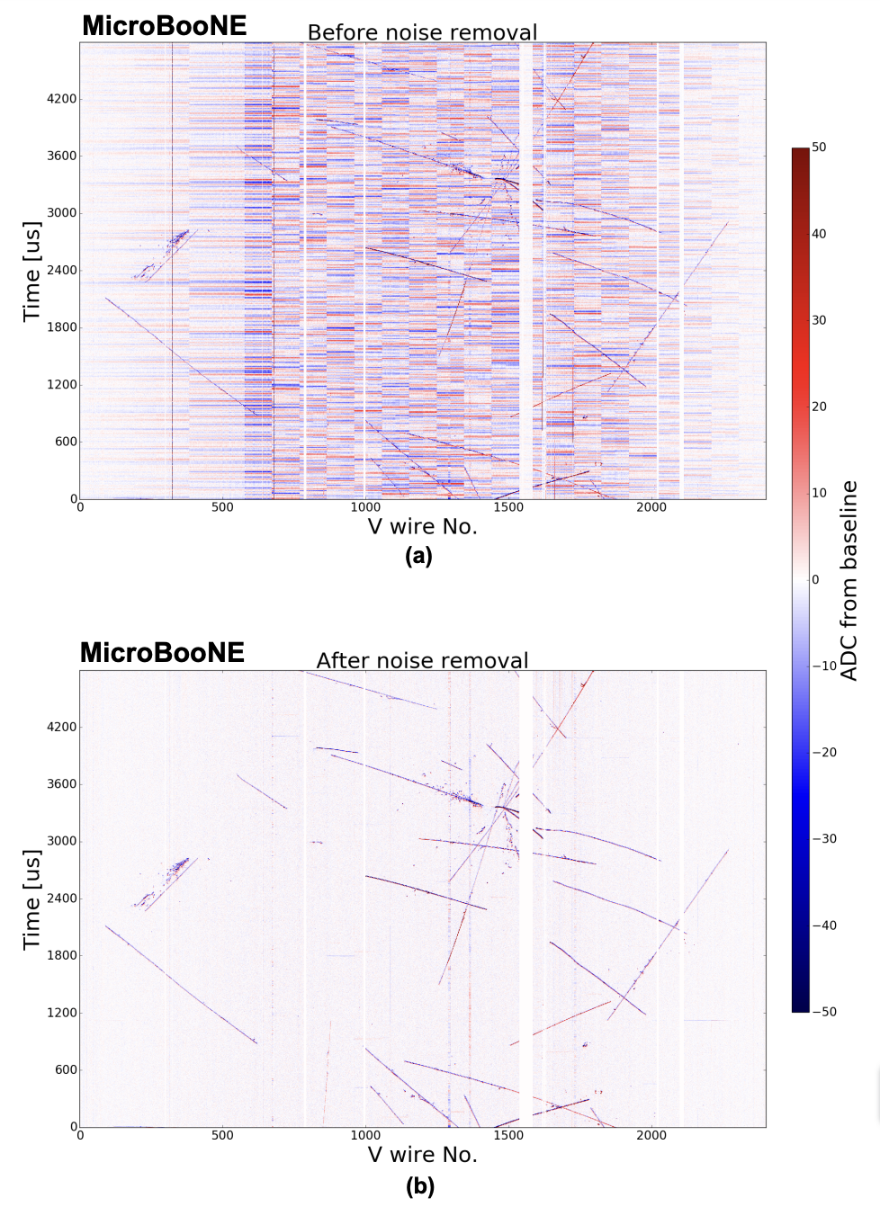
Figure 3.6: 2D displays of the signal from wires in one of the induction planes in a single data event, before and after the application of the offline noise filters. Figure from Ref. [18].

3.2.2 Deconvolution

Even after noise filtering, the signal from the TPC is a complex combination of a number of factors: the ionization electron distribution, the induced current in each wire due to passing ionization electrons, and the response of the electronics system. The signal must undergo deconvolution in order to obtain the quantity of physical interest–the number of ionization electrons passing each wire as a function of time. The signal processing algorithm designed to extract this information is described in detail in Ref. [19] and validated using MicroBooNE data in Ref. [168]. We give a brief overview of the algorithm here.

The measured signal $M(t)$ on a given wire is a convolution of the original signal $S(t^{\prime})$ and the detector response function $R(t,t^{\prime})$, which is intended to capture all the factors impacting signal formation discussed above. This can be expressed by the integral

$$M(t)=\int_{-\infty}^{\infty}R(t,t^{\prime})S(t^{\prime})dt^{\prime}.$$ (3.2)

For a time-invariant detector response function $R(t,t^{\prime})=R(t-t^{\prime})$, one can express this relationship in the frequency domain via a Fourier transform. In a realistic setup, however, this treatment tends to amplify the effect of high-frequency components of the inherent electronics noise. Typically one introduces a filter function $F(\omega)$ to suppress high frequency response, such that the original signal can be determined from

$$S(\omega)=\frac{M(\omega)}{R(\omega)}F(\omega).$$ (3.3)

In this setup, one can consider $F(\omega)$ as a replacement for the detector response function.

The filter function used in MicroBooNE is inspired by the Weiner filter [169], which is designed to optimize the signal-to-noise ratio while minimizing variance and bias and the resulting $S(\omega)$. The exact Weiner filter is not applicable in the realistic MicroBooNE setup, as it does not conserve the total number of ionization electrons and can lead to non-local charge smearing due to suppression of low frequencies [19]. MicroBooNE instead constructs a Weiner filter $F(\omega)$ from simulation, and then fits the result to a functional form designed to preserve the normalization of the measured signal and remove the unwanted low-frequency suppression behavior.

The procedure discussed so far only accounts for the signal generated in a given wire due to ionization electrons passing by that wire. In reality, electrons passing by neighboring wires can also induce a current in a given wire. This is addressed by using a two-dimensional (2D) deconvolution in both the time and wire dimensions rather than the one-dimensional deconvolution in the time dimension introduced above. An additional Weiner-inspired filter is constructed along the wire dimension when performing 2D deconvolution. After the 2D deconvolution, the algorithm identifies a region of interest (ROI) around each potential signal. These ROIs act as high-pass filters which suppress low-frequency noise in the deconvolved signal while preventing any non-local charge smearing.

The full deconvolution algorithm results in a robust reconstruction of the amount of charge passing by or deposited on each wire of the LArTPC. Figure 3.7 shows the U plane event display for a neutrino interaction candidate in MicroBooNE data after the application of the deconvolution algorithm. After the 2D deconvolution, one can clearly identify all of the charged particle tracks coming from the neutrino interaction vertex. The shape of the deconvolved signal for wires in each plane matches closely between data and simulation, as discussed in Ref. [168]. The signals produced by the deconvolution algorithm are ready to be used by MicroBooNE physics analyses, including the search for the MiniBooNE electron-like excess presented in chapters 4 and 5.

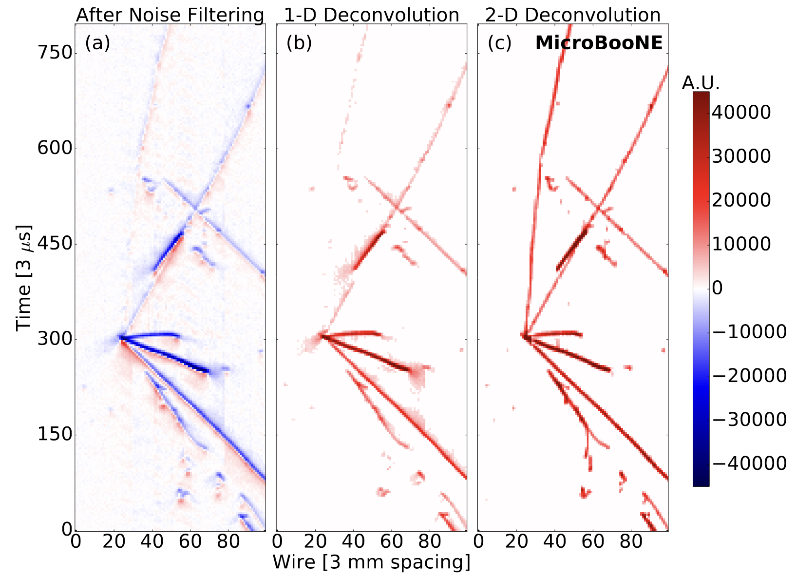
Figure 3.7: A U plane event display of a candidate neutrino interaction in the MicroBooNE data. The impact of the 1D and 2D deconvolution algorithms on the post-noise-filtering signal is shown. Figure from Ref. [19].

Chapter 4 The MicroBooNE Electron Neutrino Analysis: Overview and Selection

The MicroBooNE experiment was conceived to investigate the nature of the excess of low-energy electron-like events observed by the MiniBooNE experiment, described in detail in chapter 2. The MicroBooNE LArTPC, described in chapter 3, produces high-resolution event displays of neutrino interactions which enable the separation of events with electrons in the final state from those with photons. The collaboration released its first results searching for a MiniBooNE-like excess of electromagnetic events in October 2021. Four different analyses were performed, one focusing on photons and three focusing on electrons. The photon analysis searched for an excess of $\Delta\to N\gamma$ radiative decays [80]–the only SM photon background not constrained in situ by MiniBooNE. The three electron analyses searched for an excess of $\nu_{e}$ charged-current (CC) interactions, each with a different final state signal definition [116]. One of the electron analyses, hereafter referred to as the “inclusive analysis”, isolated all $\nu_{e}$ CC interactions using the WireCell reconstruction framework [170]. Another electron analysis, hereafter referred to as the “MiniBooNE-like analysis”, used the Pandora reconstruction framework to isolate all $\nu_{e}$ CC interactions without pions in the final state [171]. This chapter describes the “two-body CCQE analysis”, which used deep learning techniques to isolate charged-current quasi-elastic (CCQE) $\nu_{e}$ interactions consistent with two-body scattering [148]. The results from this analysis are presented in chapter 5. The two-body CCQE analysis represents much of my early work as a graduate student.

Publications covered in this chapter for which I either held a leading role or made major contributions: [148, 116, 172]

4.1 Dataset and Simulation

The results covered in this section come from the first $6.88\times 10^{20}$ POT of BNB data taken by the MicroBooNE experiment. These data were separated into three run periods which spanned from 2016 to 2018: run 1 ($1.75\times 10^{20}$ POT), run 2 ($2.70\times 10^{20}$ POT), and run 3 ($2.43\times 10^{20}$ POT) [148]. Data from two more MicroBooNE run periods exist on tape and are currently being processed by the collaboration, corresponding to another roughly $5\times 10^{20}$ POT. The entire dataset was taken during nominal neutrino mode running conditions for the BNB, in which 8 GeV kinetic energy protons from the Fermilab Booster strike the beryllium target to produce a cascade of mesons, and the positively-charged mesons are focused and decay to produce a beam of neutrinos. The BNB was described in detail in section 2.1.1. The intrinsic $\nu_{e}$ component of the beam, which makes up $\sim 0.5$% of the total neutrino flux, can be seen in figure 2.2.

The MicroBooNE simulation relies on the GENIE v3.00.06 [173, 174, 175, 176] neutrino event generator. MicroBooNE specifically employs the G18_10a_02_11a model, which uses the Valencia CCQE and meson-exchange-current (MEC) models [177] as well as a local Fermi gas model to describe the nuclear environment. GENIE models the final state interactions (FSI) of particles produced in neutrino interactions with the nuclear environment using the typical $A^{2/3}$ scaling, including corrections from nuclear binding energy [178] as well as Pauli blocking and the velocity dependence of the nuclear mean field [179]. To improve the nuclear modeling of CCQE and MEC interactions, MicroBooNE has developed a custom tune of the G18_10a_02_11a model using a $\nu_{\mu}$ CC$0\pi$ cross section measurement from T2K [180, 181]. This so-called “MicroBooNE tune” was determined by performing a two-dimensional fit of the T2K double-differential cross section data in muon momentum $p_{\mu}$ and angle $\cos\theta_{\mu}$. The fit adjusts four parameters related to the CCQE and MEC cross section models in GENIE v3.00.06, resulting in a better fit to both T2K and MiniBooNE double-differential cross section data (though discrepancies exist at lower muon momenta in the latter case). The MicroBooNE tune is used for all three MicroBooNE $\nu_{e}$ analyses; it gives better agreement with MicroBooNE $\nu_{\mu}$ data, which are essential for constraining the $\nu_{e}$ prediction in each analysis, and updates the predicted $\nu_{e}$ CCQE and MEC cross sections on argon [180].

Electron scattering data can be used to evaluate the vector part of the vector-axial neutrino-nucleus cross section models in event generators such as GENIE v3.00.06 [182, 183]. Earlier versions of GENIE were found to be in disagreement with electron scattering data in the sub-GeV energy transfer regime [182]. Updates to the QE, MEC, and $\Delta$ excitation models in GENIE improved agreement with the QE peak and MEC-dominated dip region, though disagreements remain at higher momentum transfers [183]. Dedicated electron scattering measurements using the CLAS detector at Jefferson Lab have also revealed biases in the GENIE-based reconstruction of the incident electron energy, especially in the large final state transverse momentum regime [184].

Particle propagation in the liquid argon detector is handled by the Geant4 toolkit V10.3.03c [185], and the MicroBooNE TPC response is modeled using the general LArSoft [186] package and the internal uboonecode package. The effect of cosmic particles crossing the TPC during the readout window is modeled by overlaying off-beam data on top of the simulated events. This is important, as around 20-30 cosmic rays can cross the detector in a single event due to the long readout window and near-surface location of the MicroBooNE detector [148].

4.2 The Electron Low Energy Excess Template

The hypothesis studied in each of the three electron analyses is that the MiniBooNE anomaly comes from an excess of $\nu_{e}$ interactions from the BNB. While such an excess could come from $\nu_{\mu}\to\nu_{e}$ oscillations in a $3+1$ model, this is not the only possible source. For example, mismodeling of $\mu^{+}$ decay-in-flight and $K^{+}$ decay-at-rest in the BNB [14] could lead to an enhancement of low energy $\nu_{e}$ compared with the expectation.

MicroBooNE has elected to remain agnostic about possible sources of $\nu_{e}$ events for its first results. To do this, the collaboration has developed an “electron low energy excess (eLEE) model” by unfolding the MiniBooNE excess under a $\nu_{e}$ hypothesis [148, 20]. This is accomplished using the D’Agostini iterative unfolding procedure [187], which updates a predicted distribution in true space using an observed distribution in reconstructed space and a known detector response matrix connecting the two. The algorithm relies on Bayes theorem to update the predicted distribution over a specified number of iterations. A small number of iterations will give an unfolded distribution biased toward the initial guess, while a larger number of iterations will give an unfolded distribution that is more sensitive to statistical fluctuations in the observed data [20]. For the eLEE model, the MiniBooNE observation as a function of reconstructed neutrino energy, as shown in figure 2.5, is used to unfold the predicted $\nu_{e}$ interaction rate in MiniBooNE as a function of the true neutrino energy. This procedure accounts for the detection efficiency; thus, the unfolded distribution can be interpreted as the number of $\nu_{e}$ events that interact in MiniBooNE. One can take the ratio of the unfolded MiniBooNE $\nu_{e}$ prediction to the nominal $\nu_{e}$ prediction from the MiniBooNE Monte Carlo (MC), as shown in figure 4.1(a). This gives a set of binned weights as a function of the true $\nu_{e}$ energy, which can be applied to any BNB MC sample of $\nu_{e}$ interactions to represent a MiniBooNE-like excess. These weights constitute the MicroBooNE eLEE model of the MiniBooNE anomaly. Figure 4.1(b) shows the actual eLEE model weights used in all three MicroBooNE $\nu_{e}$ analyses, calculated using the first $12.84\times 10^{20}$ POT of the MiniBooNE neutrino mode dataset.

A few comments are necessary regarding the unfolding procedure. First, the number of iterations is a regularization parameter that must be selected by the user. MicroBooNE used three iterations of the D’Agostini algorithm to produce the eLEE model, a choice designed to minimize the variance and bias in the unfolded spectrum while remaining in good agreement with the MiniBooNE data, i.e. retaining a $\chi^{2}$ per degree-of-freedom less than 1 in the reconstructed distribution. While it is true that these criteria select a unique choice for the number of iterations, the eLEE model shown in figure 4.1(b) is not the unique unfolded distribution consistent with the MiniBooNE excess. This point is discussed further in Ref. [188]. Additionally, the eLEE model was developed before MiniBooNE had looked at any $\nu_{e}$ data in the $E_{\nu}^{\rm QE}<200\;{\rm MeV}$ region [79]. Thus, the unfolded $\nu_{e}$ prediction will lose events that reconstruct below 200 MeV. It is also worth noting that while the MiniBooNE $e$-like dataset is only sensitive in principle to $\nu_{e}$ CC interactions without pions in the final state (as both charged and neutral pions are visible in a Cherenkov detector), the eLEE model weights are applied to all $\nu_{e}$ CC interactions in MicroBooNE. The impact of this choice is mitigated by the development of three different $\nu_{e}$ analyses with an emphasis on different final states. If the MiniBooNE excess only exists in one class of $\nu_{e}$ interactions, this should be evident when comparing results from all three analyses. Finally, the eLEE model does not account for systematic uncertainties on the MiniBooNE prediction. This is important, as MiniBooNE is a systematics-limited experiment [10]. The eLEE model weights shown in figure 4.1(b) can be thought to represent a “median” model of the MiniBooNE excess. One can scale the weights by an overall factor, hereafter referred to as the “LEE signal strength” $x_{\rm LEE}$, to capture the 21% statistical $\mathop{\oplus}$ systematic normalization uncertainty on the MiniBooNE prediction. In chapter 5, we will cover results from a one-dimensional signal strength scaling test.

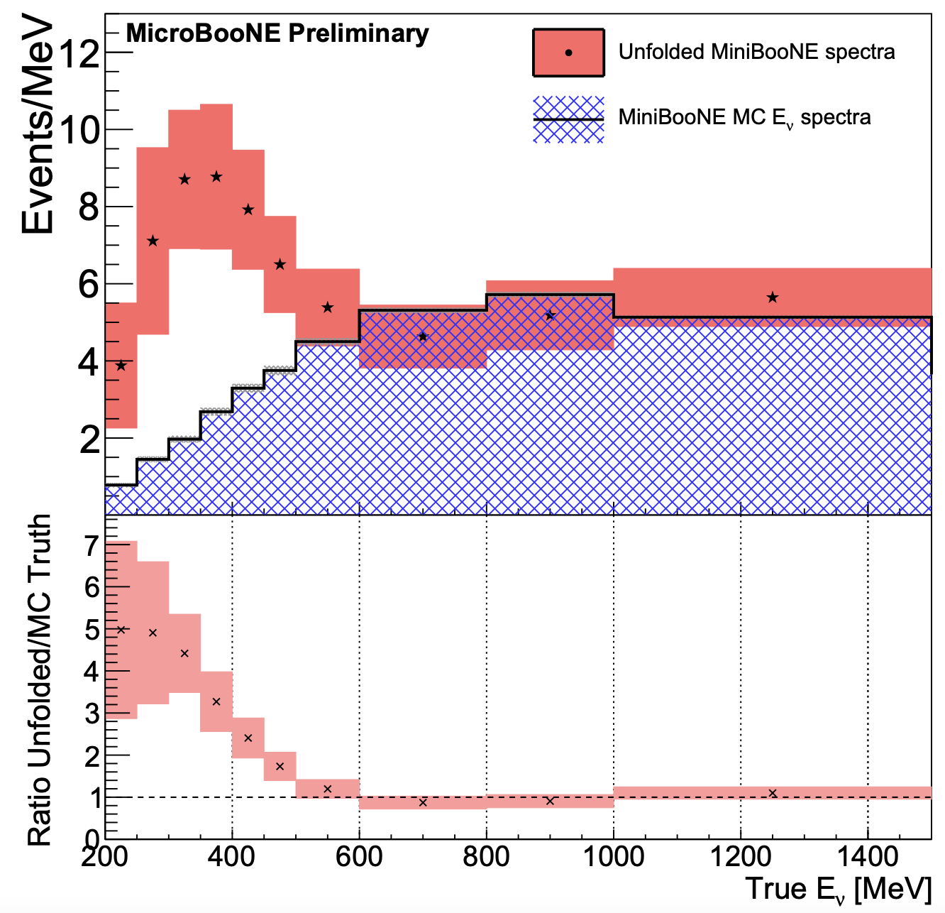
(a) From Ref. [20]

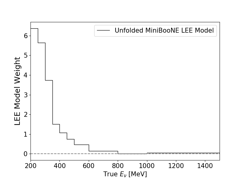
(b)

Figure 4.1: Figure 4.1(a) shows the unfolded $\nu_{e}$ prediction in MiniBooNE calculated using the first $6.46\times 10^{20}$ POT of neutrino mode data [20]. Figure 4.1(b) shows the unfolded eLEE model weights derived from the first $12.84\times 10^{20}$ POT of MiniBooNE neutrino mode data, which constitute the MicroBooNE eLEE model.

4.3 Philosophy Behind the Two-Body CCQE Analysis

The two-body CCQE analysis seeks to do what MiniBooNE could not–isolate a high-purity sample of $\nu_{e}$ interactions with a low SM photon background, especially at low energies. To do this, we have selected a very specific final state definition: $\nu_{e}$ CCQE interactions with reconstructed kinematic variables that are consistent with two-body scattering.

The $\nu_{\ell}$ CCQE interaction channel is a simple two-body scattering process,

$$\nu_{\ell}n\to\ell p.$$ (4.1)

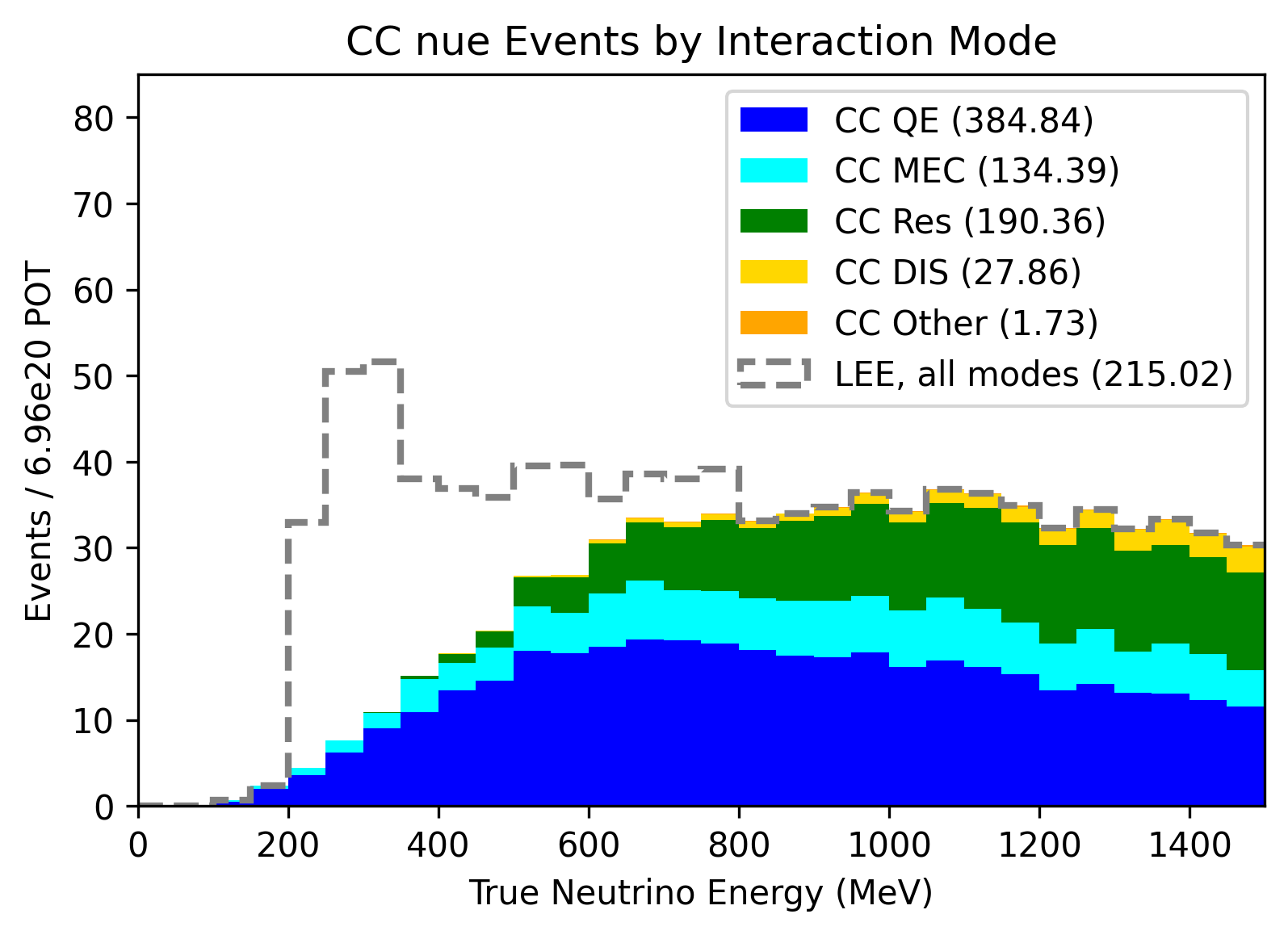
Figure 4.2: The expected distribution of $\nu_{e}$ interactions in MicroBooNE as a function of the true $\nu_{e}$ energy. The dotted line shows the expectation from the MicroBooNE eLEE model of the MiniBooNE excess discussed in section 4.2.

It was chosen because CCQE is the dominant neutrino interaction at lower neutrino energies, where the eLEE model weights in figure 4.1(b) are the highest. As shown in figure 4.2, CCQE interactions comprise 77% of the $\nu_{e}$ CC interactions in MicroBooNE below 500 MeV [148]. Other interaction channels, such as meson exchange current (MEC) and resonant (RES) scattering, become more significant at higher neutrino energies. These channels are much more complicated than CCQE and thus come with larger modeling uncertainties. MEC events involve pion exchange between two nucleons and are thus sometimes referred to as “two-particle-two-hole” interactions [189]. RES events involve the excitation of a nucleon to a $\Delta$ resonance which will subsequently decay, most often to a pion and nucleon. CCQE events are also easier to reconstruct; the original neutrino energy is simply the sum of the observed electron and proton kinetic energies, up to smearing from nuclear effects. In MEC and RES events, one must account for the kinetic energy of additional final state protons and pions, and the potential existence of invisible final state neutrons makes it more difficult to connect the total kinetic energy of the observed final state to the initial neutrino energy. Thus, the relative simplicity of CCQE interactions is another advantage of choosing such a signal definition.

The two-body CCQE analysis has developed a number of techniques to isolate $\nu_{e}$ CCQE events from other $\nu_{e}$ and $\nu_{\mu}$ interactions in MicroBooNE. The most basic of these involves leveraging the clean $1e1p$ final state topology of the signal events. The left panel of figure 4.3 shows an example candidate $1e1p$ event in MicroBooNE data. One can clearly see the proton track and electron EM shower emanating from the same vertex, presumably the location of the neutrino interaction in the LArTPC. Our reconstruction algorithm takes advantage of this distinct “vee” shape, imposing a strict requirement that exactly two “prongs” of charge (i.e., tracks or showers) come from the same 3D-consistent interaction vertex. This process is augmented by a powerful convolutional neural network to specifically find events with one track and one shower, indicative of a $1e1p$ final state. The reconstruction algorithm for this analysis will be discussed in more detail in the next section.

We also rely on two-body kinematics to select $\nu_{e}$ CCQE interactions. In theory, the observed $1e1p$ final state from a $\nu_{e}$ CCQE interaction should obey kinematic constraints imposed in a two-body scattering process. In a realistic MicroBooNE scenario, the struck neutron lives within the argon nuclear medium and has non-zero initial momentum. The final state proton must also travel through the argon nuclear medium, in which it can undergo final state interactions that alter its momentum and/or create additional hadronic particles. In order to optimize our reconstruction and minimize uncertainties, we are interested in events with minimal final state interactions. We also want to remove backgrounds that will be especially inconsistent with two-body kinematics, such as $\nu_{e}$ MEC events and $\nu_{\mu}$ events with a $\pi^{0}$ in the final state in which one of the photons is reconstructed alongside a proton track. This is achieved by introducing variables to the analysis that are especially sensitive to deviations from two-body kinematics. For example, the total transverse momentum of the neutrino interaction ($p_{T}$) will be further from zero for non-CCQE events. Additionally, as shown in figure 4.4, the proton in a two-body CCQE scattering interaction will always be forward-going. While nuclear effects can in principle break this requirement in MicroBooNE, it is much more likely for a non-CCQE background event to result in a backward-going proton than a true CCQE event. Therefore, we explicitly require forward-going protons in this analysis. We can also consider the Bjorken scaling variable

$$x_{Bj}=\frac{Q^{2}}{2p_{p}\cdot q},$$ (4.2)

where $q^{2}=-Q^{2}$ is the four-momentum transfer and $p_{p}$ is the final state proton four-momentum. In the case of quasi-elastic scattering, $x_{Bj}$ should be close to unity up to nuclear effects [190], while it can significantly differ from unity for non-CCQE backgrounds [148].

Finally, we can harness the full power of the LArTPC technology to reconstruct the $\nu_{e}$ energy in multiple ways. For $\nu_{e}$ traveling along the $z$ axis of the detector, the neutrino energy can be calculated from any of the following,

$$E_{\nu}^{\rm range} =\textnormal{K}_{p}+\textnormal{K}_{\ell}+M_{\ell}+M_{p}-(M_{n}-B),$$ (4.3)

$$E_{\nu}^{QE-p} =\left(\dfrac{1}{2}\right)\/\dfrac{2\cdot(M_{n}-B)\cdot E_{p}-((M_{n}-B)^{2}+M_{p}^{2}-M_{\ell}^{2})}{(M_{n}-B)-E_{p}+\sqrt{(E_{p}^{2}-M_{p}^{2})}\cdot\cos\theta_{p}},$$ (4.4)

$$E_{\nu}^{QE-\ell} =\left(\dfrac{1}{2}\right)\/\dfrac{2\cdot(M_{n}-B)\cdot E_{\ell}-((M_{n}-B)^{2}+M_{\ell}^{2}-M_{p}^{2})}{(M_{n}-B)-E_{\ell}+\sqrt{(E_{\ell}^{2}-M_{\ell}^{2})}\cdot\cos\theta_{\ell}},$$ (4.5)

where $K_{\ell/p}$ is the kinetic energy of the lepton or proton, $\theta_{\ell/p}$ is the angle of the shower or track with respect to the $z$ axis, $M_{\ell/p/n}$ is the particle mass, and $B$ is the average binding energy, which is around 40 MeV in argon [191]. For a true $\nu_{e}$ CCQE interaction, all three of these formulae should yield a similar reconstructed neutrino energy. To leverage this effect we define the “QE consistency” variable $\Delta^{QE}$ as

$$(\Delta^{QE})^{2}\equiv(E_{\nu}^{\rm range}-E_{\nu}^{QE-p})^{2}+(E_{\nu}^{\rm range}-E_{\nu}^{QE-\ell})^{2}+(E_{\nu}^{QE-\ell}-E_{\nu}^{QE-p})^{2},$$ (4.6)

which should be close to zero for CCQE events. To mitigate smearing from nuclear effects, $E_{\nu}^{QE-p}$ and $E_{\nu}^{QE-\ell}$ are calculated in the rest frame of the struck nucleon. We note here that equation 4.3 is the official reconstructed neutrino energy used for this analysis; $E_{\nu}$ and $E_{\nu}^{\rm range}$ are used interchangeably throughout this thesis.

Finally, it is worth mentioning that the two-body CCQE analysis also isolates a control sample of $\nu_{\mu}$ CCQE interactions with a $1\mu 1p$ final state. The $1\mu 1p$ sample is constructed analogously to the signal $1e1p$ sample, though with around two orders of magnitude more events (as $\nu_{\mu}$ comprise most of the BNB flux). This sample is used to constrain the intrinsic $\nu_{e}$ prediction and uncertainties in the $1e1p$ sample, as the $\nu_{e}$ and $\nu_{\mu}$ flux and cross section are highly correlated. We also make use of dedicated $\pi^{0}$ and Michel electron samples, as will be discussed in section 4.4.3.

In summary, the goal of the analysis presented here is the isolation of clean two-body $\nu_{e}$ CCQE interactions in MicroBooNE. The following sections explain how we leverage the topological and kinematic patterns described above to identify such events.

Figure 4.3: An example candidate $1e1p$ data event in MicroBooNE, including the raw LArTPC collection plane image (left) and the pixel labels assigned from SparseSSNet (right).

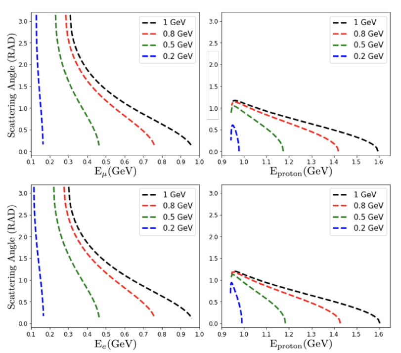
Figure 4.4: The relationship between the final state lepton (left) and proton (right) energy and scattering angle, for different neutrino energies, in $\nu_{\mu}$ (top) and $\nu_{e}$ (bottom) CCQE scattering.

4.4 Reconstruction

We begin with a broad overview of the reconstruction chain for the two-body CCQE analysis. An initial set of neutrino event candidates are identified by requiring sufficient light detection in time with the beam trigger, as discussed in section 3.1.3. These events are passed through the noise filter and deconvolution algorithm described in section 3.2 and shown in figure 3.7. Additionally, a “good runs cut” is employed to remove events during which the MicroBooNE detector response was especially noisy [148]. These steps are common to all MicroBooNE analyses. They result in one event display per wire plane for every event, similar to the rightmost panel of figure 3.7 and the left panel of figure 4.3. The color axis in the left panel of figure 4.3 is given in “pixel intensity units” (PIU), which are defined as the integrated charge in one wire over six 0.5 $\mu$s time ticks [148]. Given the electron drift speed of 0.11 cm/$\mu$s, this corresponds to a spatial extent of 0.33 cm along the drift direction. The wire spacing is such that each pixel in the left panel of figure 4.3 represents a $0.3$ cm $\times$ $0.33$ cm 2D square in the detector.

In the two-body CCQE analysis, these event displays are first passed through the sparse semantic segmentation network (SparseSSNet) [21]. SparseSSNet is a custom convolutional neural network (CNN) developed by the analysis team that labels the active pixels in each event according to five different charge deposition hypotheses: highly-ionizing particle (HIP), minimum-ionizing particle (MIP), EM activity, delta electron, or Michel electron. For the purposes of this analysis, we group HIP and MIP labels into the parent “track” label and EM activity, delta electrons, and Michel electrons into the parent “shower” label. An example SparseSSNet label is shown in the right panel of figure 4.3.

After going through SparseSSNet, the images are filtered for crossing cosmic interactions using the WireCell charge-to-light matching algorithm [192, 193]. This algorithm matches charge observed on the TPC to light observed by the PMTs to identify regions of charge which are not coincident in time with the beam spill, presumably coming from cosmic rays. We can then mask these pixels to remove the bulk of cosmic-related charge deposition. The cosmic-filtered SparseSSNet output is then used as input to a vertex and track identification algorithm, which looks for a shower-like and track-like prong of charge coming from a given 3D vertex [24]. Track-like prongs pass through a dedicated step of the algorithm that performs a step-by-step 3D reconstruction of the extent and direction of the track, which is then translated into a range-based energy and angle estimation. The events are then passed through a dedicated EM shower identification algorithm that identifies cones of shower-like pixels pointing back to the neutrino interaction vertex and estimates the total visible energy and angle of the shower. [172]. This algorithm has the capability of finding up to two showers separated from the vertex, which is necessary for identifying events with a $\pi^{0}\to\gamma\gamma$ decay.

After finding candidate neutrino vertices, we pass the event displays through the multiple particle identification (MPID) CNN [22]. This network assigns five scores to each image indicating the network’s confidence that the event contains a proton, electron, muon, photon, or charged pion. The MPID scores are not used until the final signal selection described in section 4.5.

At this point, the reconstruction chain has identified two-prong candidate events and reconstructed the relevant lowest-level kinematic variables of each final state particle, i.e. the energy and direction. These kinematic variables are then combined to calculate more complicated kinematic variables such as $Q^{2}$, $p_{T}$, $x_{Bj}$, and the reconstructed $\pi^{0}$ mass (in the case of two-shower events), as well as the most important variable in this analysis: the reconstructed neutrino energy $E_{\nu}^{\rm range}$, as defined in equation 4.3. The full suite of reconstructed kinematic variables used to define the $1e1p$ and $1\mu 1p$ samples is given in table 4.1. These variables are used as input to the signal selection described in section 4.5. The following subsections explain in more detail the most important steps of the reconstruction procedure.

Variable Name	Definition
Base Variables
$\textnormal{K}_{p}$	Kinetic energy of proton determined from range [24]
$\textnormal{K}_{\ell}$	Kinetic energy determined from range for muons [24] and from calorimetry for electrons  [172]
$M_{\ell}$, $M_{n}$, $M_{p}$	Masses of the lepton, neutron and proton
$\cos{\theta_{p}}$, $\cos{\theta_{\ell}}$	$p_{p}^{z}/p_{p}$, $p_{\ell}^{z}/p_{\ell}$
$\phi_{p}$, $\phi_{\ell}$	$atan2(p_{p}^{y},p_{p}^{x})$,  $atan2(p_{\ell}^{y},p_{\ell}^{x})$
$P_{p}=(E_{p},p_{p})$, $P_{\ell}=(E_{\ell},p_{\ell})$	Reconstructed 4-vector of the proton, lepton
$B$	Binding Energy for argon; the analysis assumes $B=40$ MeV
Definitions Related to Neutrino Energy
$E_{\nu}^{range}$ (Default value of $E_{\nu}$)	$\textnormal{K}_{p}+\textnormal{K}_{\ell}+M_{\ell}+M_{p}-(M_{n}-B)$
$E_{\nu}^{QE-p}$	$\big{(}\dfrac{1}{2}\big{)}\/\dfrac{2\cdot(M_{n}-B)\cdot E_{p}-((Mn-B)^{2}+M_{p}^{2}-M_{\ell}^{2})}{(M_{n}-B)-E_{p}+\sqrt{(E_{p}^{2}-M_{p}^{2})}\cdot\cos\theta_{p}}$
$E_{\nu}^{QE-\ell}$	$\big{(}\dfrac{1}{2}\big{)}\/\dfrac{2\cdot(M_{n}-B)\cdot E_{\ell}-((Mn-B)^{2}+M_{\ell}^{2}-M_{p}^{2})}{(M_{n}-B)-E_{\ell}+\sqrt{(E_{\ell}^{2}-M_{\ell}^{2})}\cdot\cos\theta_{\ell}}$
$\Delta^{QE}$ (2-Body Consistency)	$\sqrt{(E_{\nu}^{range}-E_{\nu}^{QE-p})^{2}+(E_{\nu}^{range}-E_{\nu}^{QE-\ell})^{2}+(E_{\nu}^{QE-\ell}-E_{\nu}^{QE-p})^{2}}$
Event Kinematics
$Q^{2}$	$2E_{\nu}^{range}(E_{\ell}-P_{\ell}^{z})-M_{\ell}^{2}$
Hadronic Energy (Ehad)	$E_{\nu}^{range}-E_{\ell}$
Björken’s Scaling x (xBj)	$Q^{2}/2M_{n}E_{had}$
Björken’s Scaling y (yBj)	$E_{had}/E_{\nu}^{range}$
Opening angle	$\cos^{-1}(\hat{p}_{\ell}\cdot\hat{p}_{p})$
$p_{T}$	$\sqrt{(p_{\ell}^{x}+p_{p}^{x})^{2}+(p_{\ell}^{y}+p_{p}^{y})^{2}}$
$p_{L}$	$p_{p}^{z}+p_{\ell}^{z}$
$\alpha_{T}$	$\cos^{-1}\left(-\dfrac{\vec{P}_{T}^{l}\cdot\vec{P}_{T}}{|\vec{P}_{T}^{l}||\vec{P}_{T}|}\right)$
$\phi_{T}$	$\cos^{-1}\left(-\dfrac{\vec{P}_{T}^{l}\cdot\vec{P}_{T}^{p}}{|\vec{P}_{T}^{l}||\vec{P}_{T}^{p}|}\right)$
Boosting Parameters
$p_{fermi}^{T}$	$p_{p}^{T}+p_{\ell}^{T}$
$p_{fermi}^{z}$	$p_{p}^{z}+p_{\ell}^{z}-E_{\nu}^{range}$

Table 4.1: The definition of kinematic variables used throughout the two-body CCQE analysis.

4.4.1 Convolutional Neural Networks in LArTPCs

As discussed above, The two-body CCQE analysis relies on two CNNs to assist in reconstructing the MicroBooNE LArTPC images: SparseSSNet and MPID.

SparseSSNet is described in detail in Ref. [21]. The network uses a combination of the U-Net [194] and ResNet [195] architectures. The U-Net uses an encoding step, in which the input image is downsampled to a smaller size, followed by a decoding step, in which the encoded image is upsampled to the same dimensionality and size as the original image. This second step is required to perform pixel-level labeling. The ResNet architecture employs residual connections that improve the training performance of deeper networks compared to regular CNNs [195]. SparseSSNet also makes use of sparse submanifold convolutions [196], which perform better on semantic segmentation tasks for sparse input data like LArTPC images (where very few pixels in a given image have nonzero charge). The training sample is generated using the simulation described in section 4.1; specifically, a random set of visible final state particles are generated at randomly distributed locations within the detector. The network performs considerably well on the nominal MicroBooNE BNB simulation sample, as well as the dedicated intrinsic $\nu_{e}$ simulation sample, neither of which appeared in the SparseSSNet training sample [21]. While SparseSSNet has not been statistically evaluated against MicroBooNE data, hand scans of the network output on data event displays do not reveal any bias in the network performance [21]. The performance of an earlier iteration of SparseSSNet was evaluated using two data samples: Michel electrons and $\nu_{\mu}$ CC $\pi^{0}$ events [197]. Good agreement was observed between pixel labels in data and simulation for both samples, and no significant differences were found between network-labeled images and physicist-labeled images. Figure 4.5 shows the SparseSSNet architecture as well as an example labeled image in the training dataset.

The MPID network is described in detail in Ref. [22]. It uses a standard CNN architecture which takes as input a 2D LArTPC image cropped around the neutrino interaction candidate vertex on a single wire plane and outputs five numbers representing different particle scores for protons, electrons, muons, photons, and charged pions. The score is meant to represent the likelihood that a given particle exists in the provided image. Two types of scores are generated: an “image” score, describing the probability that the particle exists anywhere in the image, and the “interaction” score, describing the probability that the particle is connected to the neutrino interaction vertex. The training sample is generated similarly to that of SparseSSNet; random sets of particles are generated throughout the detector volume with energies in a range relevant to MicroBooNE. The MPID score distributions exhibit excellent agreement between data and simulation in two different samples: $\nu_{\mu}$ CC $1\mu 1p$ events and $\nu_{\mu}$ CC $\pi^{0}$ events [22]. Figure 4.6 shows the MPID architecture as well as an example simulated image with MPID image scores.

It is also worth briefly mentioning energy reconstruction in LArTPCs using CNNs. My earliest work as a graduate student investigated the ability of the ResNet [195] and Inception network [198] CNN models to reconstruct EM shower energies in MicroBooNE. Compared to the standard clustering-based shower reconstruction algorithm described in section 4.4.3, the CNN method appeared to better handle EM showers that passed through unresponsive wires in the MicroBooNE detector. Despite the promise of the CNN method, it was not developed in time to be implemented in the two-body CCQE analysis. Nevertheless, the MicroBooNE-specific network was extended by an MIT undergraduate, Kiara Carloni, to enable a systematic study of CNN-based EM shower energy reconstruction in a general LArTPC [23]. The corresponding publication is included in Appendix A. Figure 4.7 shows the main takeaway of this work: a CNN-based reconstruction method is significantly more robust to unresponsive wires in the detector compared with a traditional EM shower reconstruction algorithm, which employs a linear calibration between the total shower charge and energy.

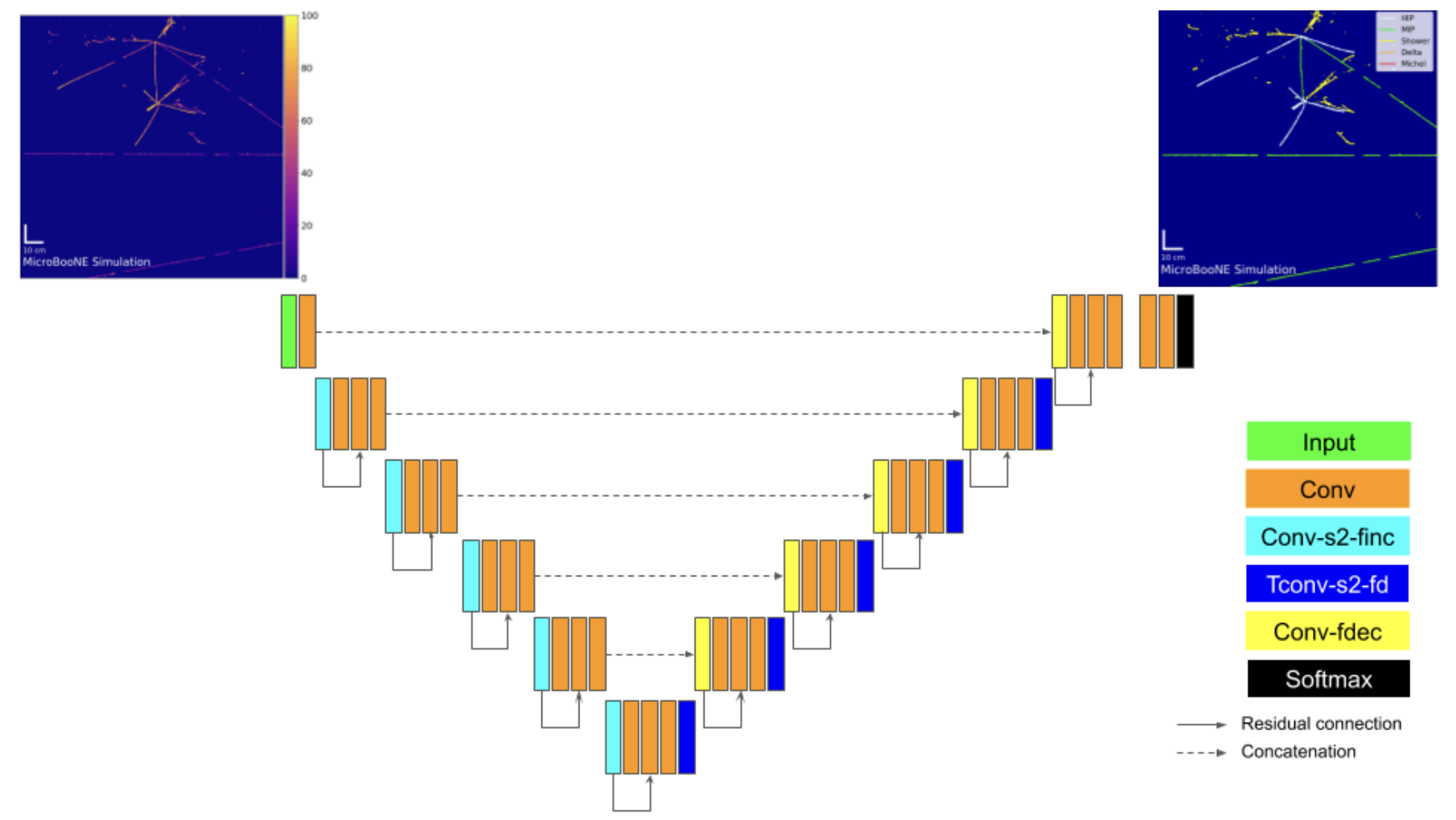
(a)

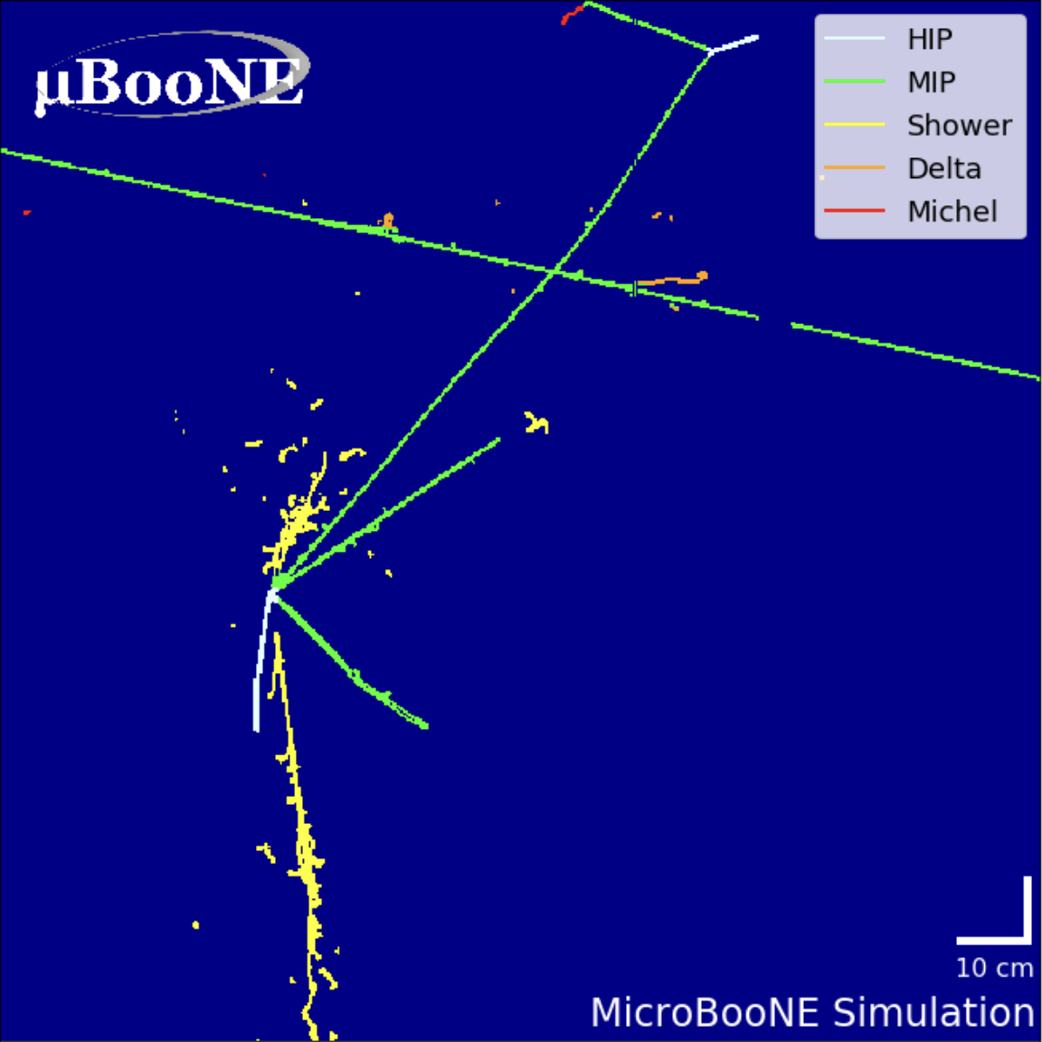
(b)

Figure 4.5: Figure 4.5(a) shows a diagram of the SparseSSNet U-ResNet architecture. Figure 4.5(b) shows the SparseSSNet pixel labels on a simulated image in the training dataset. Figures from Ref. [21].

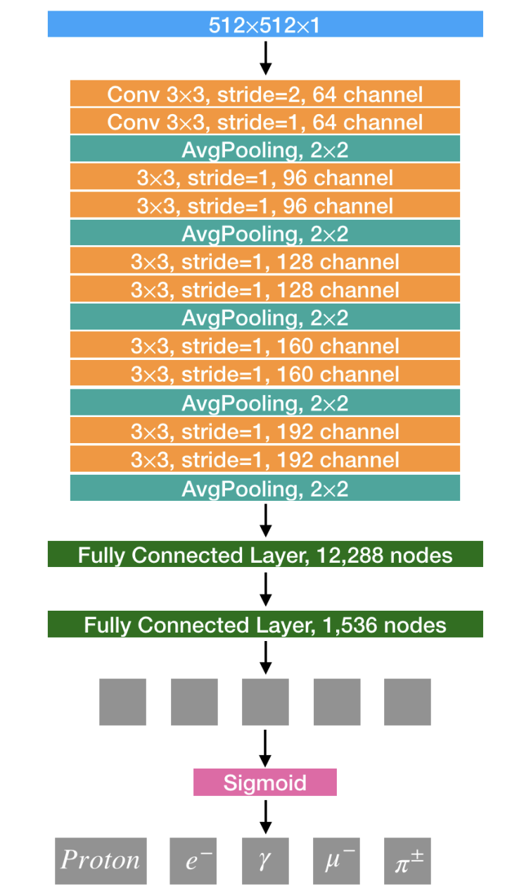
(a)

(b)

Figure 4.6: Figure 4.6(a) shows a diagram of the MPID architecture. Figure 4.6(b) shows the MPID image scores on an example simulated event. Figures from Ref. [22].

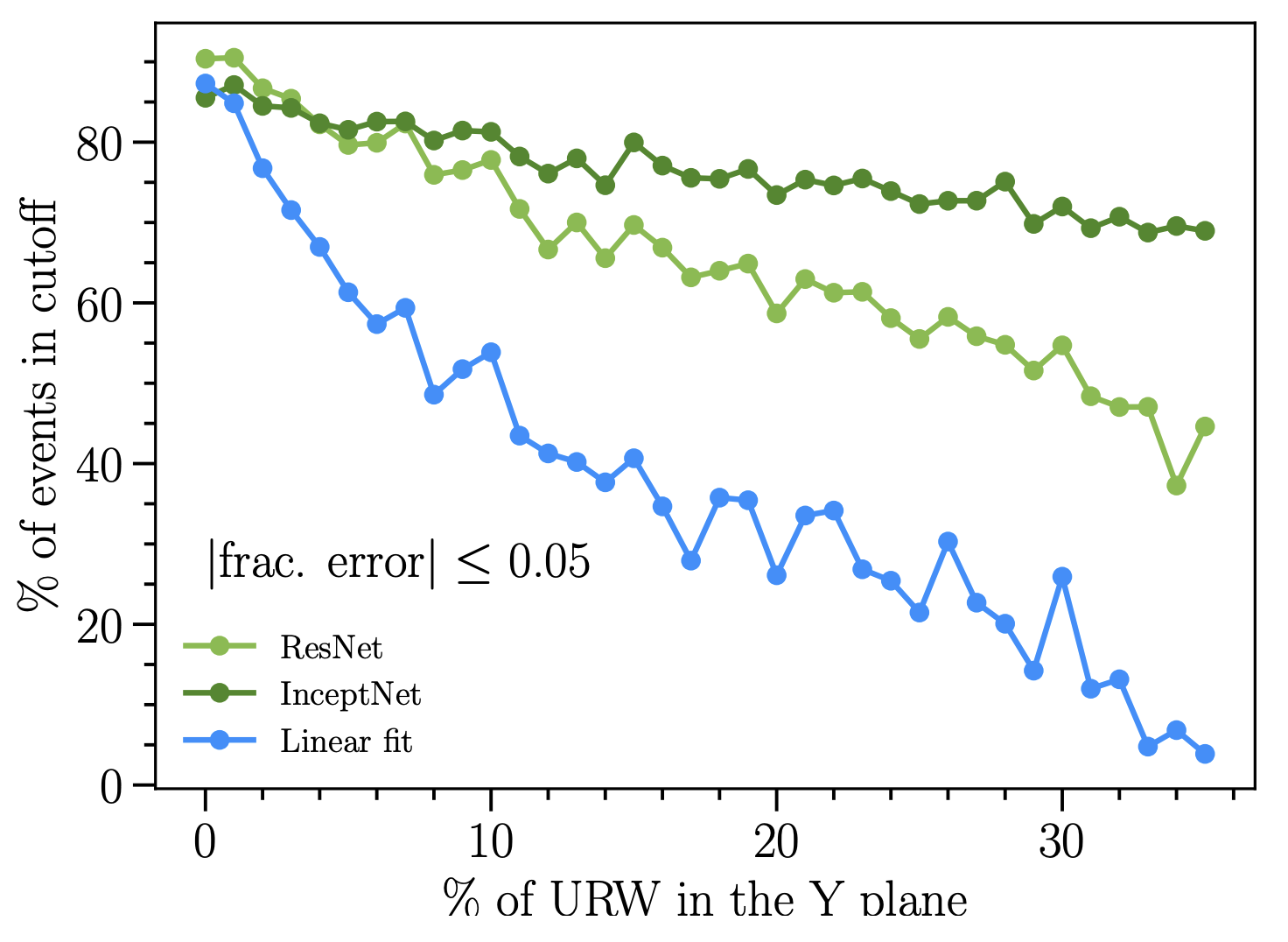
Figure 4.7: The fraction of EM showers reconstructed to within 5% of the true deposited energy as a function of the fraction of unresponsive wires in the LArTPC collection plane, considering three different methods. The ResNet and Inception network significantly outperform the traditional linear calibration between charge and energy. Figure from Ref. [23].

4.4.2 Vertex and Track Reconstruction

After running SparseSSNet and filtering cosmic-associated charge, the images are passed through the vertex reconstruction algorithm described in Ref. [24]. In brief, the algorithm looks for the characteristic “vee” shape of both $1e1p$ signal events, as shown in the left panel of figure 4.3, and $1\mu 1p$ control sample events. The algorithm begins by isolating a sample of 2D vertex seeds (i.e., candidate neutrino interaction locations) on each plane. This is done by clustering regions of charge and then applying two techniques–contour defect identification using a convex hull and intersection identification using principal component analysis. The set of vertex seeds is reduced to those that are consistent in the time dimension across all three planes. From each triplet of time-consistent vertex seeds on the three wire planes, a final 3D vertex is found by minimizing an angular metric that represents the likelihood that two clusters of charge emanate radially from that vertex location. Figure 4.8(a) shows an example minimization of this angular metric, which involves calculating two different estimates of the opening angle between the two prongs for a given vertex location. Simulation studies indicate that this algorithm is able to reconstruct neutrino interaction vertices to within less than 1 cm with an average efficiency of 56% [24].

After finding a neutrino vertex candidate, we perform a 3D reconstruction of the prongs of charge emitted from the vertex [24]. An iterative stochastic algorithm identifies a set of 3D spatial points associated with each prong by building upon previous points; these points comprise the track. This process is shown diagrammatically in figure 4.8(b). It is worth noting that the “tracks” at this stage can correspond to either true tracks (HIPs and MIPs) or EM showers.

The 3D track can be projected onto each 2D plane. At this point, the SparseSSNet labels on each plane are used to determine if the event is a “track-track” or “track-shower” event. The latter case happens when greater than 20% of the pixels in a given prong are labeled as shower pixels. In the “track-shower” case, the shower-like prong is considered to be the electron while the track-like prong is the proton. Thus, these are candidate $1e1p$ events. The “track-track” case corresponds to candidate $1\mu 1p$ event, where the shorter track is ascribed to the highly-ionizing proton. Electron EM showers are not sufficiently reconstructed in this step and are left for a dedicated shower reconstruction algorithm described in section 4.4.3. Muons and protons can, however, be reconstructed at this stage. The polar and azimuth angles of each particle can be determined from the direction of the associated track. The length of the tracks is used in conjunction with the known stopping power of each particle in liquid argon to determine the kinetic energy. Simulation studies of $1\mu 1p$ events suggest an angular resolution of a few degrees and a kinetic energy resolution of a few percent [24].

It is also worth mentioning that two-prong events with an opening angle of less than 10^∘ in any plane are rejected at this point. Thus, signal events in this analysis consisted of well-separated leptons and protons.

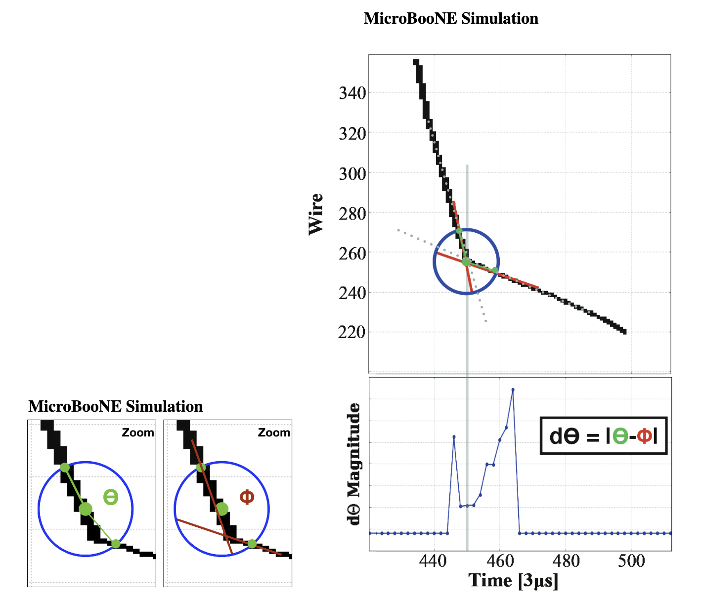
(a)

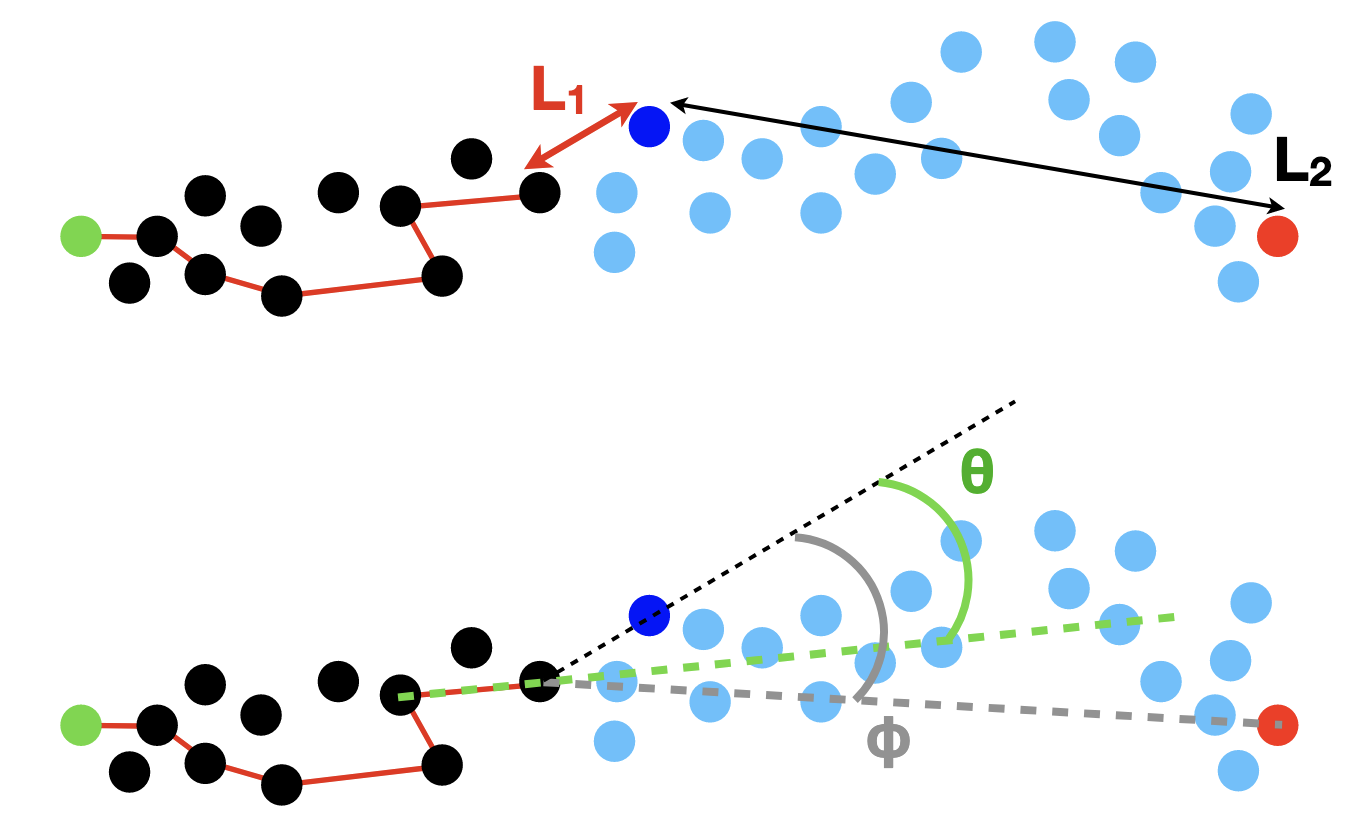
(b)

Figure 4.8: Figure 4.8(a) shows the angular metric that is minimized to find a 3D neutrino vertex candidate. Figure 4.8(b) shows the iterative track reconstruction algorithm, which relies on calculating distances (L₁ and L₂) and angles ($\theta$ and $\phi$) with respect to the previous point and the end of the track. Figures from Ref. [24].

4.4.3 Publication: Electromagnetic shower reconstruction and energy validation with Michel electrons and $\pi^{0}$ samples for the deep-learning-based analyses in MicroBooNE

As mentioned in the previous section, a dedicated algorithm is used to reconstruct the EM showers coming from the neutrino interaction vertex. The algorithm is described in detail in Ref. [172], which also covers a data-driven validation of the shower reconstruction using dedicated $\pi^{0}$ and Michel electron samples. A brief overview of the shower reconstruction is as follows. We first mask out pixels in each plane for which the SparseSSNet shower score is below a value of 0.5. Next, we attach a triangle to the interaction vertex in each plane and optimize the direction, gap from the vertex, opening angle, and length of the triangle to encapsulate as many shower pixels as possible without becoming too large. We calculate the energy of the shower by performing a linear calibration between the summed PIU in the collection plane shower triangle and the simulated electron/photon energy. The collection plane is used because it produces the most robust signals, as discussed in section 3.2. We reconstruct 3D showers by looking for overlap in the time dimension between the shower triangles on all three planes. This algorithm can be run a second time after masking out the optimized triangle from the first pass, which is essential for isolating a $\pi^{0}$ sample.

This MicroBooNE publication was led by myself and Katie Mason, a graduate student from Tufts University. Katie focused on the triangle-fitting procedure of the shower reconstruction and the $\pi^{0}$ mass peak fit, while I focused on the charge-to-energy scaling of the shower reconstruction and the Michel energy spectrum fit. The full JINST publication is included below. The most important result from this study is shown in Figure 16 of the paper, which demonstrates good agreement between the simulation-derived charge-to-energy scaling applied to EM showers in this analysis and two standard candles: the $\pi^{0}$ invariant mass peak and the cutoff of the Michel electron energy distribution.

See pages - of templates/Publications/Abratenko_2021_J._Inst._16_T12017.pdf

4.5 $1e1p$ Event Selection

The signal events for this analysis, $1e1p$ events consistent with two-body CCQE scattering, are isolated using a series of cuts on kinematic, topological, and MPID-based variables as well as an ensemble of boosted decision trees (BDTs). The $1e1p$ signal selection represents one of my main projects within the MicroBooNE experiment. This section covers in detail the requirements which define the $1e1p$ sample. The $1\mu 1p$ control sample is isolated analogously to the $1e1p$ sample and will not be covered in this thesis, though more information can be found in Ref. [148].

4.5.1 Basic Data Selection Criteria

We first apply a series of basic “precuts” meant to remove poorly reconstructed events and obvious backgrounds. We begin with the collection of “track-shower” vertices selected by the algorithm described in section 4.4.2, which represent candidate $1e1p$ events. We remove any vertices that are within 10 cm of the TPC edges or within a region of unresponsive wires between $700<z~{}[{\rm cm}]<740.$ This cut defines the fiducial volume. We also require that the minimal distance of either the track or the shower to the edge of the TPC is greater than 15 cm. In the case that both prongs are reconstructed close to an edge, we instead require that the distance of each is greater than 5 cm, which helps retain neutrino interactions that begin near the edge of the fiducial volume. Events in the $1e1p$ are further required to be outside of an inefficient region of the U-plane.

We also employ a cut requiring the reconstructed shower energy of the candidate electron to be consistent between the three planes. Even though we rely on the collection plane for the official shower energy estimation, this cut is helpful in removing events that would not lead to a consistent 3D picture of the shower. An example of such an event is shown in figure 4.9. The cut specifically employed in this analysis is

$$\frac{\sqrt{(E_{e}^{U}-E_{e}^{V})^{2}+(E_{e}^{U}-E_{e}^{Y})^{2}+(E_{e}^{V}-E_{e}^{Y})^{2}}}{E_{e}^{Y}}<2,$$ (4.7)

where $E_{e}^{[U,V,Y]}$ denote the reconstructed electron candidate energy on the $U$, $V$, and $Y$ plane, respectively. Figure 4.10(a) shows the distribution of the fractional consistency variable (left-hand side of equation 4.7) for events above and below a $1e1p$ BDT score cutoff of 0.7, where the BDT here is an older iteration of the final BDT ensemble used in this analysis. As can be seen, signal-like events (with a higher BDT score) tend to have lower fractional consistency values compared to background-like events (with a lower BDT score). The upper bound of 2 in equation 4.7 was chosen to retain $\sim 95\%$ of signal-like events while rejecting $\sim 20\%$ of background-like events, as shown in figure 4.10(b).

Next, we make cuts on the reconstructed neutrino energy ($200<E_{\nu}~{}[{\rm MeV}]<1200$), electron kinetic energy ($K_{e}>35~{}{\rm MeV}$), and proton kinetic energy ($K_{p}>50~{}{\rm MeV}$). We also require a forward-going proton and an opening angle between the electron and proton greater than 0.5 rad. Finally, we require that the event can be boosted to the rest frame of the nucleon using the $p_{fermi}^{T}$ and $p_{fermi}^{z}$ variables defined in table 4.1.

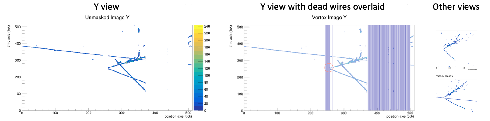
Figure 4.9: An example of an event that fails the shower energy consistency cut, because the EM shower passes through an unresponsive region of the collection plane.

(a)

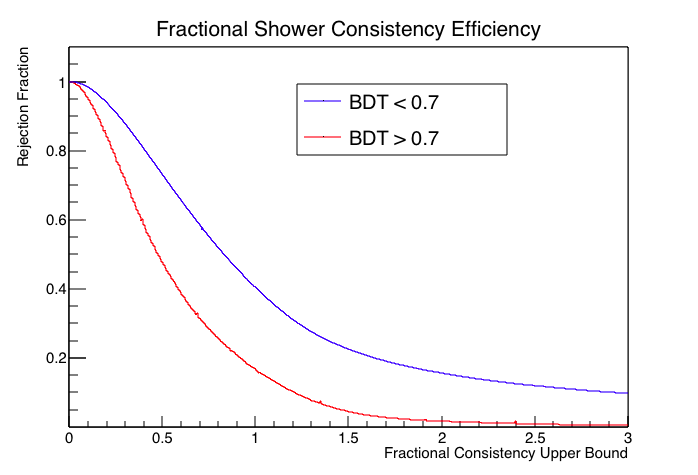
(b)

Figure 4.10: Figure 4.10(a) shows the distribution of the fractional shower energy consistency variable for events with an old $1e1p$ BDT score above/below 0.7. Figure 4.10(b) shows the efficiency with which events above/below the old $1e1p$ BDT cutoff pass the fractional consistency cut as a function of the chosen upper bound.

4.5.2 Boosted Decision Tree Ensemble

The next stage of the $1e1p$ selection uses an ensemble of BDTs to identify signal-like events in MicroBooNE. This is the most powerful cut used in the $1e1p$ analysis. The ensemble consists of 20 BDTs each trained using the XGBoost gradient-boosting algorithm [199]. Each BDT takes as input a set of 19 kinematic variables, such as the reconstructed energies and angles of the electron and proton, and 4 topological variables related to the observed charge, such as the fraction of SparseSSNet-labeled shower pixels in the event. The full suite of variables used to train the $1e1p$ and $1\mu 1p$ BDTs is shown in table 4.2. Each BDT itself consists of a collection of regression trees which each assign a continuous score to an event based on a set of decision rules developed using the input variables; the assigned BDT score of the event is given by the sum over the collection [199]. BDTs are trained via gradient-based optimization of an objective function that includes a regularization term to penalize overfitting.

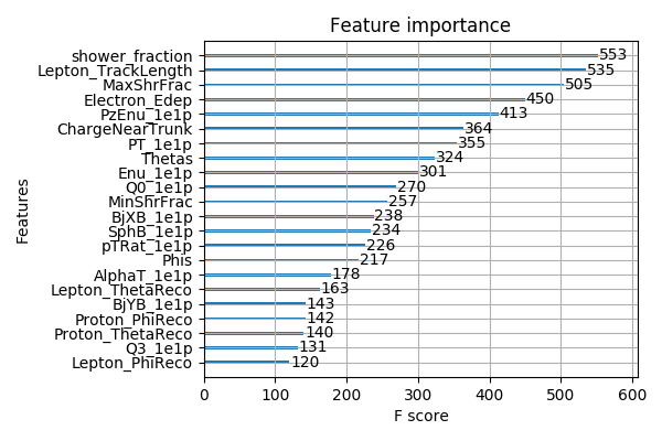
(a) Run 1

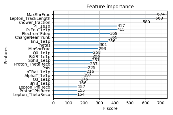
(b) Run 2

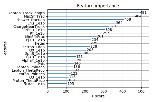
(c) Run 3

Figure 4.11: The F score of each variable for one of the $1e1p$ BDTs in the ensemble from run 1, run2, and run 3.

A different ensemble is generated for each of the three run periods, as the detector response changed slightly between them. Thus, there are 60 total BDTs trained for the $1e1p$ analysis. The BDTs are trained using the MicroBooNE MC samples, including the nominal ($\nu_{\mu}$-dominated) BNB sample as well as dedicated intrinsic $\nu_{e}$, $\pi^{0}$, and cosmic samples. The signal for the training sample is defined as true $\nu_{e}$ CCQE interactions with one electron and one proton in the final state. We further restrict to well-reconstructed events for which the vertex is reconstructed with 5 cm of the true vertex and the neutrino energy within 20% of the true value. Only non-$\nu_{e}$ CCQE $1e1p$ events are explicitly classified as background. Each BDT in an ensemble is trained using a randomly-selected half of the MC sample for the given run period. Figure 4.11 shows the F score distribution for each variable in one of the $1e1p$ BDTs from the ensemble for each run period. The F score represents the number of times each variable is used across all trees in the BDT; thus, it can be thought of as a measure of the importance of each variable.

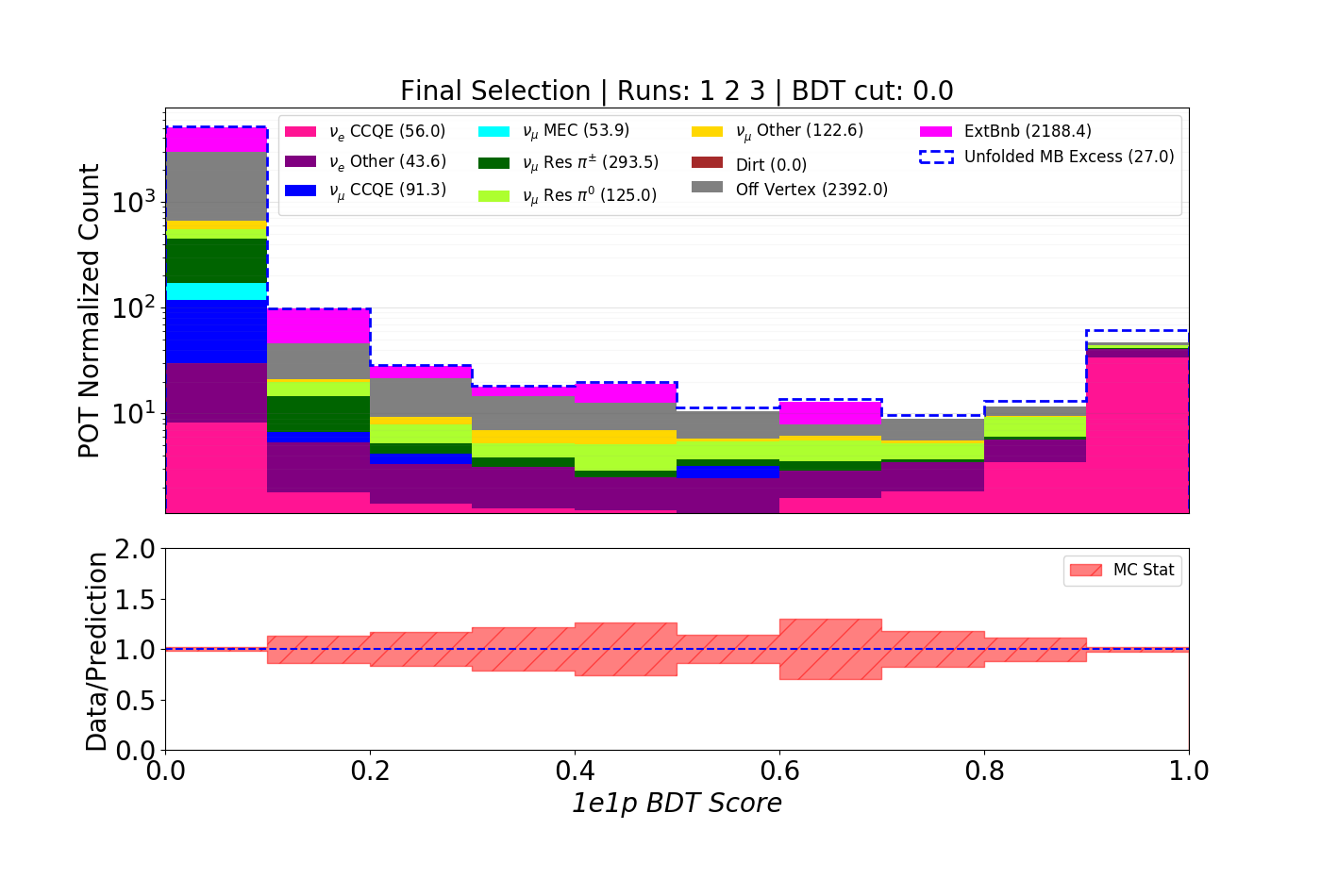
(a)

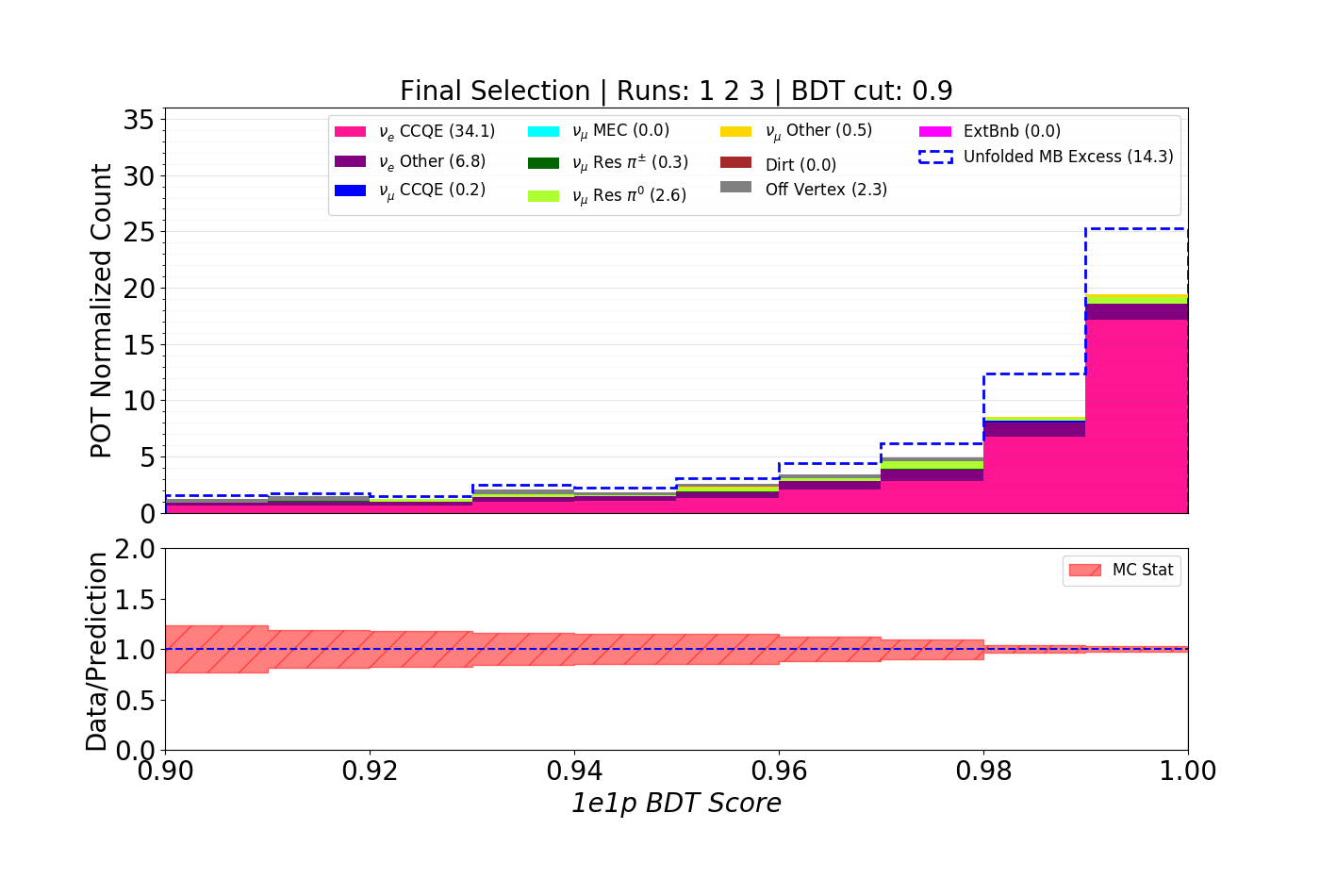
(b)

Figure 4.12: Figure 4.12(a) and figure 4.12(b) show the MC distribution of the $1e1p$ BDT ensemble average score over all three run periods for the full [0,1] range and zoomed in to the [0.95,1] range, respectively.

The $1e1p$ score for an event is evaluated by calculating the average BDT score across the ensemble. This reduces the dependence of the ensemble score on the specific training sample of any single BDT. Ensemble-based methods have been shown to reduce variance on the output likelihood variable compared to a single classifier [200]. When computing the average score for events in the MicroBooNE MC sample, we omit BDTs for which the event appeared in that BDT’s training sample. It is extremely unlikely ($p=2^{-20}$) for an event to appear in the training sample of all BDTs in an ensemble; thus, we can use the BDT ensemble to isolate a $1e1p$ signal sample prediction from the MicroBooNE MC without throwing away any events. The score is normalized to the range [0,1], where higher scores indicate a higher signal likelihood. We show the distribution of the ensemble-averaged $1e1p$ BDT score in figure 4.12, which shows that true $\nu_{e}$ CCQE events tend to peak toward 1 while all other events peak toward 0. Signal events are required to have an average score greater than 0.95, which was chosen to optimize sensitivity to the eLEE model described in section 4.2.

We have performed a series of tests of the robustness of the BDT ensemble method. We first examined the signal selection power of a BDT ensemble trained on simulated events from a given run period when used to infer the signal likelihood of simulated events from a different run period. This is useful for two reasons. For one, it provides a method for testing the ensemble on events that were in neither the training nor the validation sample of the constituent BDTs. Testing on a sample independent of the validation sample is important because the BDT training was halted when the classification error on the validation set didn’t improve after 50 training iterations. It also tests the impact of removing training events from the MC prediction. When using the BDT ensemble of a given run period to evaluate the signal likelihood of events from the same run period, one must remove events that appeared in the training sample of each constituent BDT. In this study we use the BDT ensemble trained on run period 2 to evaluate simulated $\nu_{e}$ events from run period 3 and vice versa, so one does not need to remove training events.

Figure 4.13 shows the results of this run period swap study. As one can see, the differences between the selection using the correct and incorrect run period ensemble are small. The correct run period performs slightly better, as expected due to small differences in the detector status specific to each run period. However, the relatively small change in $\nu_{e}$ selection efficiency suggests that the BDT ensemble is able to perform well on simulated events that do not appear in either the training or validation sample of constituent BDTs. One can interpret the loss in performance shown in figure 4.13 as a bound on the potential impact of applying the BDT ensemble to events that are not in the training or validation samples of the entire ensemble. The drop in performance is $<10\%$ over most of the energy range–an effect which is smaller than our systematic error before the $\nu_{\mu}$ constraint described in chapter 5 ($\sim 15\%$) and much smaller than the statistical error in each reconstructed neutrino energy bin after the final selection ($\sim$ 50%).

Next, we investigated the impact of using only a subset of the BDTs in the ensemble to calculate the average BDT score of an event. This is relevant because we omit BDTs that contained a given MC event in the training sample when calculating the average BDT score for that event. However, this analysis uses all 20 BDTs in the ensemble to calculate the average BDT score of events in the data. Therefore, to verify that comparisons between data and simulation are robust, one needs to ensure that removing BDTs from the ensemble does not significantly bias the average score calculation.

To this end, consider $S_{n}$ to be the $1e1p$ BDT ensemble average score after removing $n$ BDTs from the ensemble. For events in data, the BDT score is $S_{0}$ while for simulated events, the BDT score is $S_{n}$ for some $n\in\{1,...,20\}$. Figure 4.14 shows the fractional difference $(S_{n}-S_{0})/S_{0}$ as a function of the number of omitted BDTs $n$ over signal-like (BDT score $>$ 0.95) events in the simulation from run period 2 and run period 3, respectively. As in the previous study, in order to avoid bias from BDT training we use the BDT ensemble trained on run period 2 to evaluate the signal likelihood of simulation events from run period 3 and vice versa. The data points and error bars in figure 4.14 indicate the average and standard deviation of the fractional difference over the simulation sample, respectively. The red histograms show the actual distribution of omitted BDTs over the simulation from each run period. One can see that the average BDT score does not exhibit significant bias upon removing BDTs from the calculation. Also, the standard deviation of the fractional difference only becomes larger than $1$% when removing $\gtrsim 17$ BDTs from the calculation. This only happens for $<<1$% of simulated events, as expected.

Variable	Used in $1\mu 1p$ BDT	Used in $1e1p$ BDT
Variables Used in BDTs, Based on Ionization
Charge within 5 cm of vertex	Yes	Yes
Shower charge in event image /
shower charge clustered as electron	No	Yes
Proton shower fraction	No	Yes
Electron shower fraction	No	Yes
Variables Used in BDTs, Related to Energy Measurements
Neutrino Energy	Yes	Yes
Energy of electromagnetic shower	No	Yes
Lepton length	Yes	Yes
Proton length	No	Yes
$p_{z}-E_{\nu}$	No	Yes
Variables Used in BDTs, Related to 2-Body Scattering Consistency
Bjorken’s $x$	Yes *	Yes *
Bjorken’s $y$	Yes *	Yes *
QE Consistency	Yes *	Yes *
$Q_{0}$	Yes	Yes
$Q_{3}$	Yes	Yes
Variables Used in BDTs, Related to Transverse Momentum
$\alpha_{T}$	Yes	Yes
Event $p_{T}$	Yes	Yes
Event $p_{T}/p$ (“PTrat")	Yes	Yes
$\phi_{T}$	Yes	No
Variables Used in BDTs, Related to Angles
Proton $\phi$	Yes	Yes
Proton $\theta$	Yes	Yes
Lepton $\phi$	Yes	Yes
Lepton $\theta$	Yes	Yes
$\phi_{p}-\phi_{\ell}$	Yes	Yes
$\theta_{p}+\theta_{e}$	No	Yes
Variables Useful for Comparison, Not Used in Either BDT
$\eta$ (Normalized average ionization difference)	No	No
Opening Angle	No	No
$x$ Vertex	No	No
$y$ Vertex	No	No
$z$ Vertex	No	No

Table 4.2: The suite of variables used to isolate and analyze the $1e1p$ and $1\mu 1p$ samples. Variables used in the BDT ensemble for each sample are specified. The “$*$” character indicates that the variable is calculated in the rest frame of the struck nucleon. The mathematical definitions of many of these variables appear in Table 4.1.

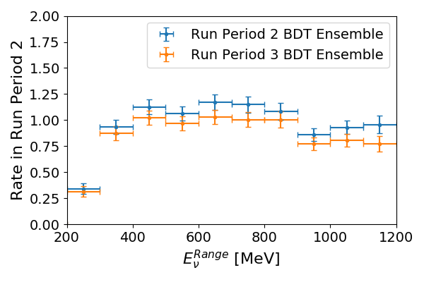
(a)

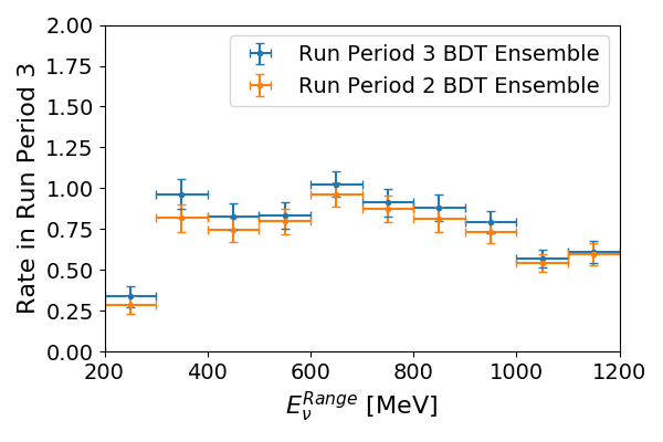
(b)

Figure 4.13: Figure 4.13(a) and figure 4.13(b) show the predicted $\nu_{e}$ event rate in run period 2 and run period 3, respectively, using both the run period 2 ensemble and the run period 3 ensemble.

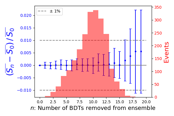
(a)

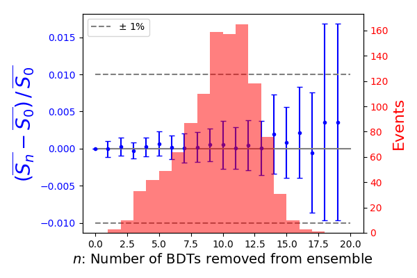
(b)

Figure 4.14: Figure 4.14(a) and figure 4.14(b) show the fractional difference in average BDT score $(S_{n}-S_{0})/S_{0}$ as a function of the number of omitted BDTs $n$ over the simulation from run period 2 and run period 3, respectively. The red histogram shows the actual distribution of the number of omitted BDTs over the run period 2 and run period 3 simulation samples, respectively. Scores are calculated using the run period 3 and run period 2 BDT ensemble, respectively.

4.5.3 Particle Identification Cuts

Finally, we employ a series of particle-identification requirements to clean up the remaining backgrounds that survive the $1e1p$ BDT ensemble cut. The first of these is a cut on the invariant $\pi^{0}$ mass. If the shower reconstruction algorithm described in section 4.4.3 is able to identify a second EM shower, the reconstructed $M_{\pi^{0}}$ must be less than 50 MeV. Another cut requires the ratio of the MPID $\gamma$ and $e^{-}$ image scores to be less than 2. This helps remove remaining $\pi^{0}$ events that survive the $M_{\pi^{0}}$ cut. We also require the MPID muon interaction score to be less than 0.2, which helps remove $\nu_{\mu}$ CC$\pi^{0}$ events where the muon gets mistaken for a proton. This last cut is only applied for events in which $E_{e^{-}}>100$ MeV, as MPID tends to assign low electron scores and high muon scores to true electrons below 100 MeV, as shown in figure 4.15. This is because electrons stop radiating below this energy, becoming more track-like and thus difficult to distinguish from muons. The specific values used for the cuts described here were chosen by optimizing the signal-to-background ratio in the $1e1p$ sample. Finally, if an event has more than one reconstructed neutrino vertex candidate passing all selection criteria, we keep only the vertex with the highest $1e1p$ ensemble BDT score.

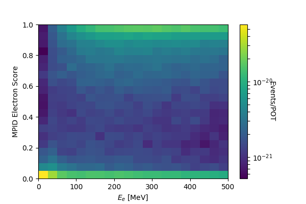
(a)

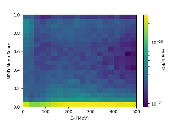
(b)

Figure 4.15: Figure 4.15(a) and figure 4.15(b) show the MPID electron and muon score, respectively, as a function of the reconstructed electron energy in intrinsic $\nu_{e}$ MC events.

4.5.4 The Final $1e1p$ Sample

The requirements described throughout this section define the $1e1p$ sample; they are summarized and compared with those in the $1\mu 1p$ sample in table 4.3. This results in a highly-pure $1e1p$ signal sample–75% of events are true $\nu_{e}$ CCQE interactions. Figure 4.16 shows the predicted $E_{\nu}^{\rm range}$ distribution for this sample, including the prediction from the eLEE model. This figure also shows the systematic uncertainty and non-$\nu_{e}$ background prediction, which will be discussed further in chapter 5. The neutrino energy distribution in figure 4.16 forms the basis of the statistical results discussed in chapter 5.

The neutrino energy resolution is 16.5% for selected $1e1p$ events, as shown in figure 4.17. This figure also indicates a slightly higher rate of events with under-predicted neutrino energy, owing mainly to showers and tracks that pass through unresponsive regions of the detector. Figure 4.18 reports the signal efficiency and total number of $\nu_{e}$ CCQE events in this sample after applying each of the three sets of cuts. The efficiency peaks at lower neutrino energies $\sim 300$ MeV, which is optimal for testing the eLEE model. Note that these efficiencies in figure 4.18(a) are reported with respect to all identified vertices. If we include the effect of the vertex algorithm, the average efficiency for retaining signal events in the $1e1p$ sample is 6.6% [148]. This is by design–in choosing a very exclusive signal definition, we optimize for a high-purity sample at the price of lower efficiency.

Name/Description of Code	Requirement for $1\mu 1p$	Requirement for $1e1p$
Cuts/Selections Applied in External Code
Common Optical Filter	$>20$ PMT hits w/i 6 ticks in beam window	Same
	& $\leq 20$ hits w/i 6 ticks in 2 $\mu s$ prior to spill
WC tagger	Mask cosmic-associated charge	Same
Preselection Cuts for Event Selection
Run Quality Requirements:
Good Run Flag	True	Same
Vertex Requirements:
$1\ell 1p$ consistent	Two prongs of at least 5cm length, no additional prongs	Same
Edge fiducial	$>10$ cm from active volume edge	Same
No dead region	outside $z=700$ to 740 cm	Same
Containment Requirements:
Edge containment	closest approach $>15$ cm from edge	Same
Efficient region	N/A	outside $y=(1/\sqrt{3})*z-117$
		to $y=1/\sqrt{3}*z-80$ cm.
Particle Energy Requirements:
Neutrino energy (range-based)	$E_{\nu}<1200$ MeV	Same
Lepton kinetic energy	$K_{\ell}>35$ MeV	Same
Proton kinetic energy	$K_{p}>50$ MeV	Same
Analysis Orthogonality Cut	Max Shower Frac $<0.2$	Max Shower Frac $>0.2$
Other Basic Quality Requirements:
Opening Angle	$>0.5$ radians	Same
Proton $\theta$	$\cos(\theta_{p})>0$	Same
Boostable	$\gamma>1$, $0<|\beta|<1$	Same
Shower 3-view energy consistency	N/A	Inconsistency $<$ 200%
Vertex with BDT score that is	lowest (i.e. best)	highest (i.e. best)
BDT Requirements for Event Selection
BDT requirement	$\nu_{\mu}$ BDT $<0.4$	$\nu_{e}$ BDT $>0.95$
PID Requirements for Event Selection
$\pi^{0}$ mass	N/A	$\pi^{0}$ mass $<50$ MeV
muon MPID interaction score	N/A	$<$ 0.2 if $E_{e}>100$ MeV
$\gamma/e$ image score ratio	N/A	$<2$
proton MPID interaction (max of 3 planes)	$>0.9$ if $E_{\nu}<400$ MeV	N/A

Table 4.3: The specific used to define the $1\mu 1p$ and $1e1p$ samples. For definitions of kinematic variables, see Table  4.1.

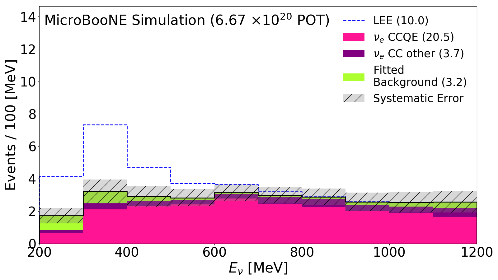
Figure 4.16: The $E_{\nu}^{\rm range}$ distribution for the $1e1p$ signal sample, showing only the predicted event rate from the MC. The prediction from the eLEE model is shown in the dashed blue line.

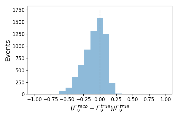
(a)

(b)

Figure 4.17: Figure 4.17(a) shows the distribution of the fractional error on the neutrino energy for MC events in the $1e1p$ signal sample, restricted to $200<E_{\nu}^{\rm Range}\;[{\rm MeV}]<1200$. Figure 4.17(b) shows the 2D distribution of fractional error as a function of the true neutrino energy.

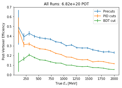
(a)

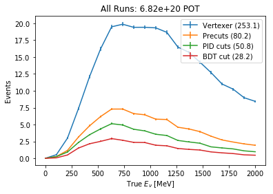
(b)

Figure 4.18: Figure 4.18(a) shows the post-vertex-identification efficiency of true $\nu_{e}$ CCQE selection for subsequent stages of the $1e1p$ cuts. Figure 4.18(b) shows the true $\nu_{e}$ CCQE event rates over the full run 1-3 dataset after subsequent stages of the $1e1p$ cuts.

Chapter 5 The MicroBooNE Electron Neutrino Analysis: Results and Discussion

This chapter presents the first results from the two-body CCQE analysis described in chapter 4. They come from data taken during the first three MicroBooNE run periods, corresponding to $6.67\times 10^{20}$ POT after data quality cuts. The signal data were examined for the first time in Summer 2021 and presented to the community in October 2021 [148]. The results from the two-body CCQE analysis were accompanied by results from the inclusive [170] and MiniBooNE-like [171] $\nu_{e}$ analyses. All three MicroBooNE $\nu_{e}$ analyses are summarized in Ref. [116].

This chapter focuses on the statistical results from the $\nu_{e}$ two-body CCQE analysis. We cover the background prediction, systematic error evaluation, $\nu_{\mu}$ $1\mu 1p$ constraint procedure, and blinded analysis approach in detail. We then discuss the series of statistical tests performed using our $1e1p$ signal sample. We close with a discussion of the MicroBooNE results, including a presentation of two non-MicroBooNE publications examining the implications of the MicroBooNE data under two different explanations of the MiniBooNE LEE: $3+1$ oscillations and excess $\overline{\nu}_{e}$ interactions.

Publications covered in this chapter for which I either held a leading role or made major contributions: [148, 116, 102, 201]

5.1 First Results from the Two-Body CCQE Analysis

The two-body CCQE analysis observed 25 events across data from the first three run periods. This is in good agreement with the total prediction in the $200-1200$ MeV range, which is $27.4\pm 3.8_{\rm sys}\pm 5.2_{\rm stat}$ before the $1\mu 1p$ constraint discussed in section 5.1.3 [148]. One of these events is shown in figure 5.1, including both pixel intensity images from the TPC readout and SparseSSNet pixel-labeled images on all three planes. Event displays for the remaining 24 selected events are included in Appendix B. The $E_{\nu}^{\rm range}$ distribution of these events is shown in figure 5.2, where the prediction is given both in terms of the underlying interaction type and the final state event topology. The $1e1p$ BDT ensemble average score distribution is shown in figure 5.3. Figure 5.4 shows the distributions of four more interesting variables: $E_{e}$, $E_{p}$, $\theta_{e}$, and $E_{\nu}^{QE-\ell}$. A full suite of data-prediction comparisons in 36 variables is provided in the Supplemental Material for Ref. [148], including those described in table 4.1 and those used to train the BDT ensembles.

One can see clearly in figure 5.2 that no excess of $\nu_{e}$ $1e1p$ candidate events is observed at low energy in the two-body CCQE analysis. Instead, we observe a slight deficit compared to even the nominal prediction at low energies, in conflict with the eLEE model represented by the blue dashed line. This is a trend that is observed across all three $\nu_{e}$ analyses in MicroBooNE [116]. The extent to which we agree or disagree with the eLEE model will be discussed further in section 5.2.

One might also notice an apparent excess of data events in the 800-900 MeV bin in figure 5.2. This appears to be a statistical fluctuation; other kinematic variables do not exhibit such an excess of events, including the closely related $E_{\nu}^{QE-\ell}$ distribution shown in figure 5.4(d). If this were a systematic effect rather than a fluctuation, one would expect similar behavior in the distributions of other variables. While these statements will be quantified further in section 5.2, it is useful to include such a qualitative discussion at this point.

The following subsections discuss the details behind our prediction in the $E_{\nu}$ distribution. It is important to note that while we have already shown the observed data in our signal channel, the procedures outlined in the following subsections were frozen before examining this dataset. Specifically, we followed the blinded analysis approach outlined in section 5.1.4 to avoid biasing our selection.

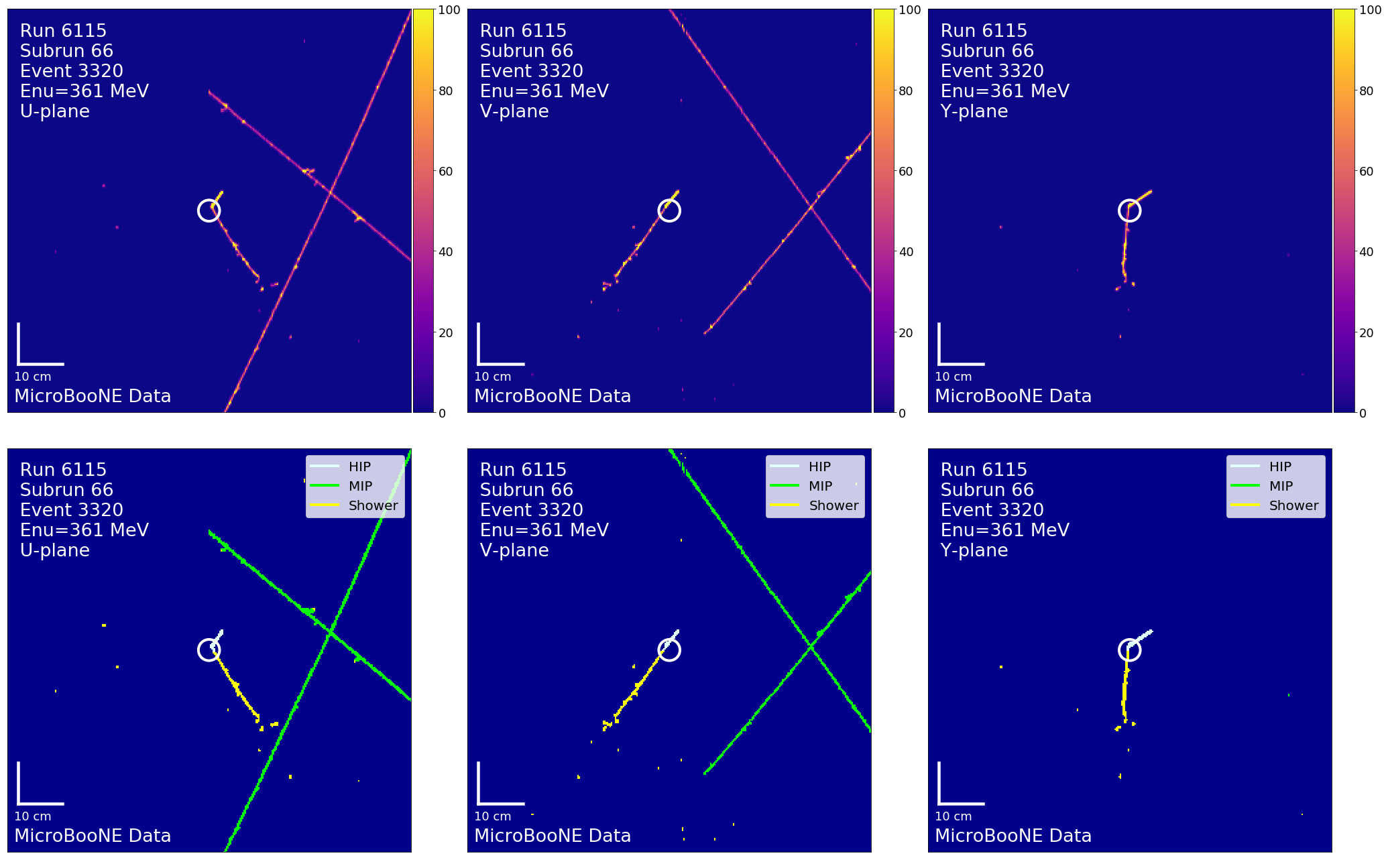
Figure 5.1: Top: pixel intensity (color scale is in PIU as defined in section 4.4); Bottom: SparseSSNet labels; Left to Right: U, V, Y, planes. The white circle indicates the reconstructed vertex. The horizontal axis corresponds to the wire plane direction and the vertical axis corresponds to the electron drift direction, which is measured using the arrival time of charge on the wires.

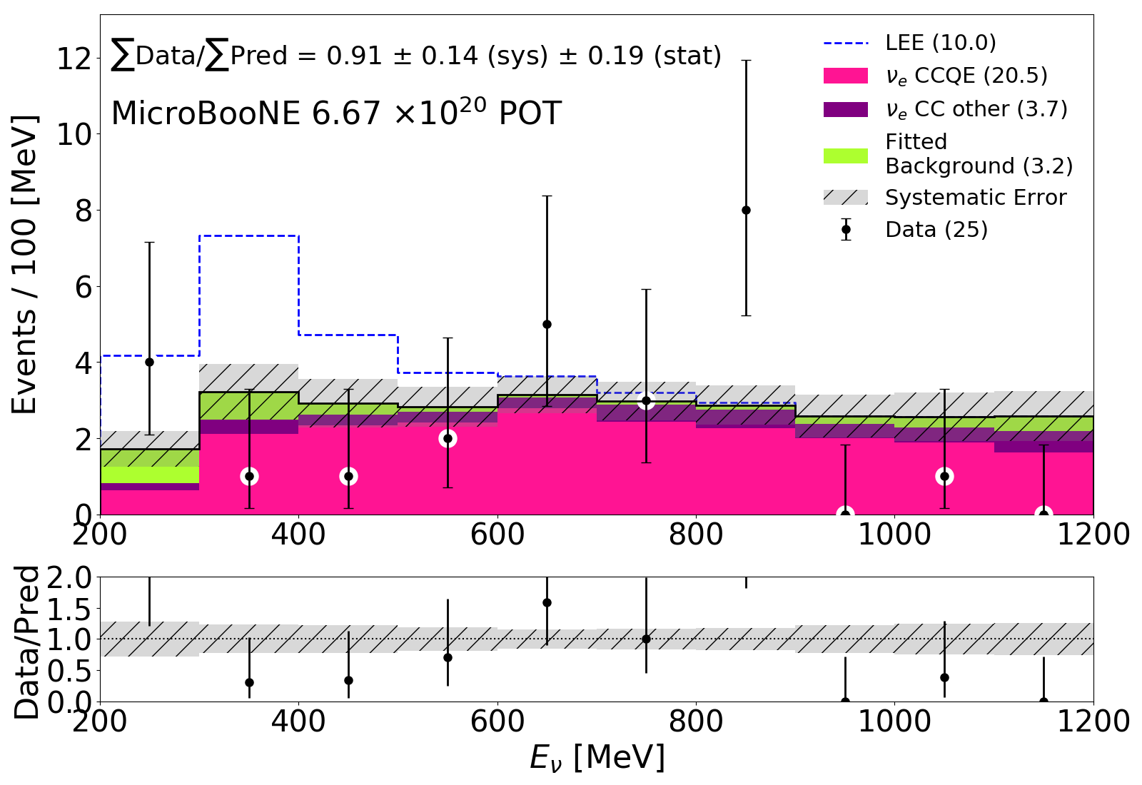
(a)

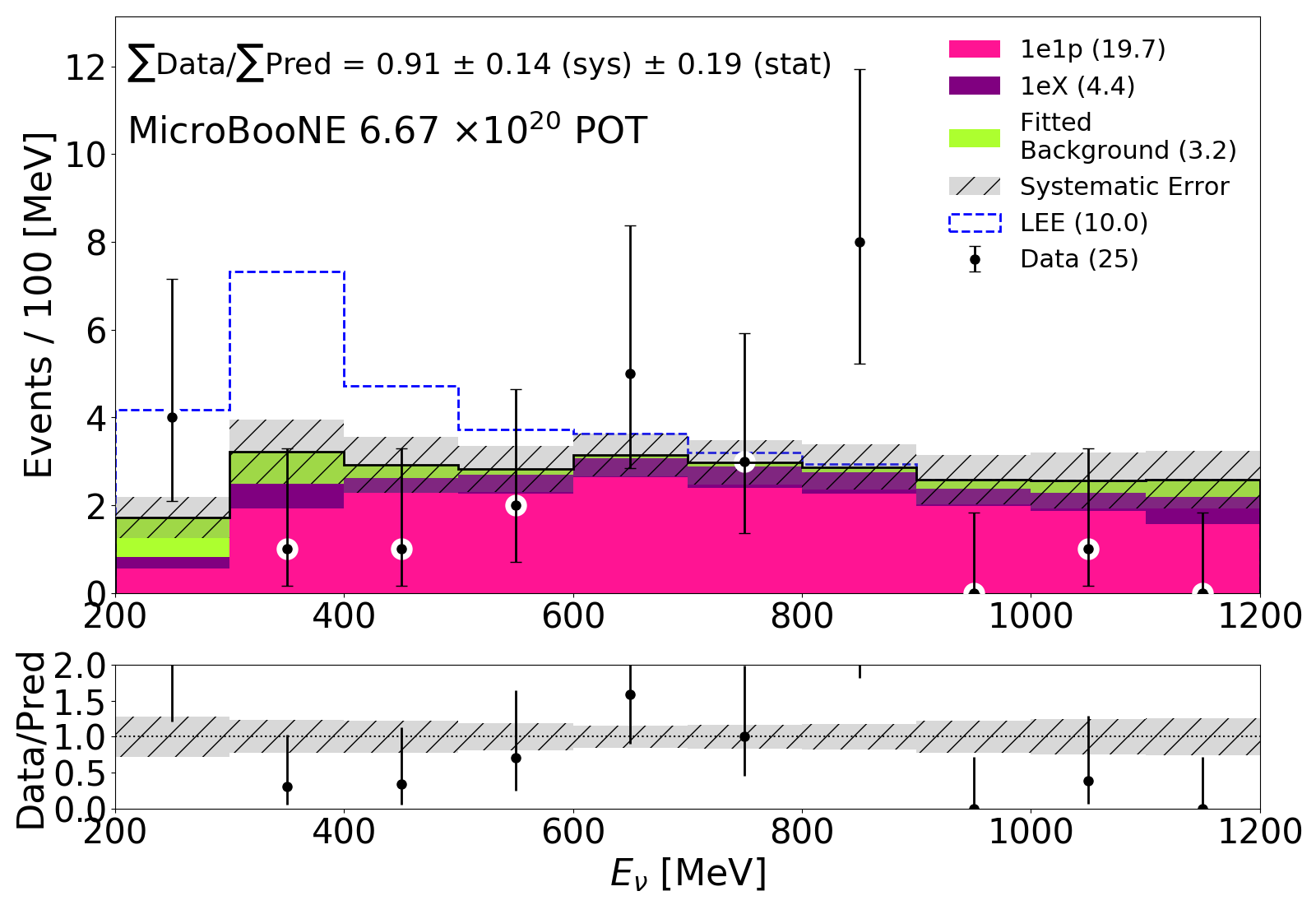
(b)

Figure 5.2: The $1e1p$ sample $E_{\nu}$ distribution, comparing data (black points) to the unconstrained prediction (stacked histogram) in the $200<E_{\nu}<1200$ MeV region. The eLEE model prediction is represented by the dashed blue line. The prediction is presented in terms of both interaction type (figure 5.2(a)) and final state topology (figure 5.2(b)).

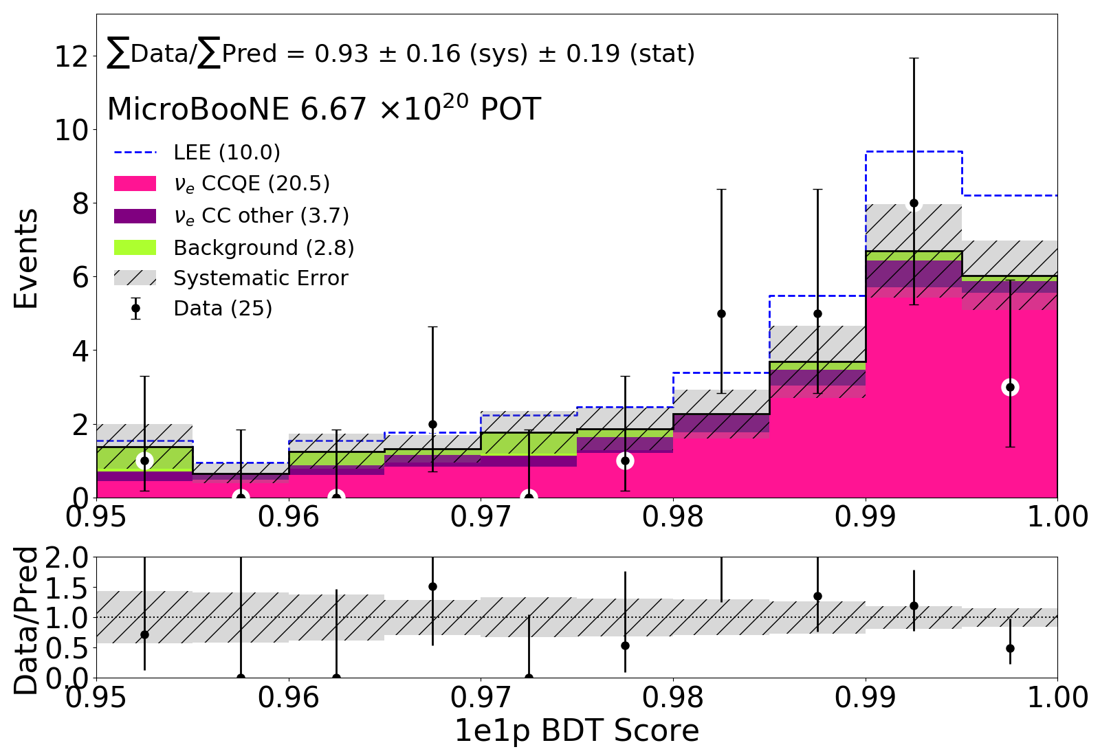
Figure 5.3: Average $1e1p$ BDT ensemble score distribution comparing data to the unconstrained prediction.

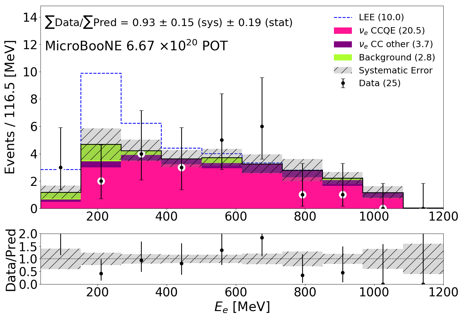
(a)

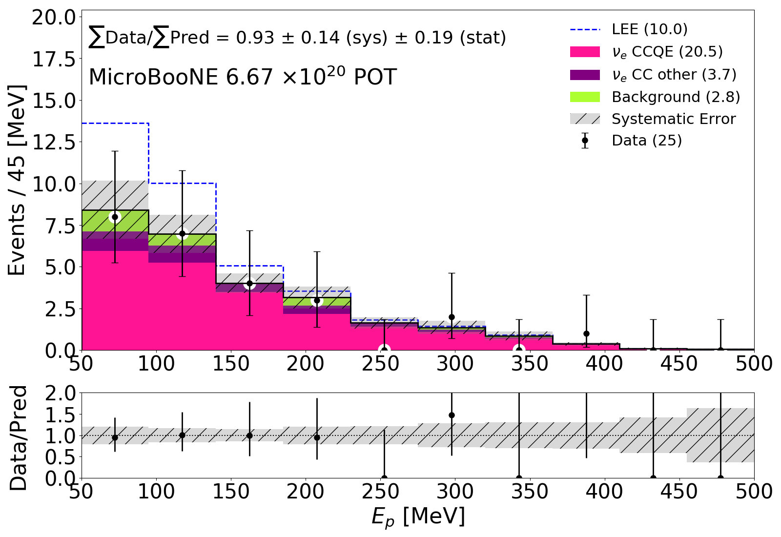
(b)

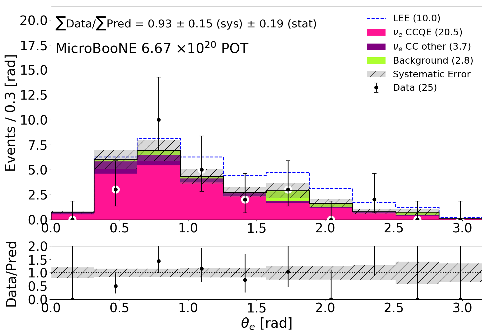
(c)

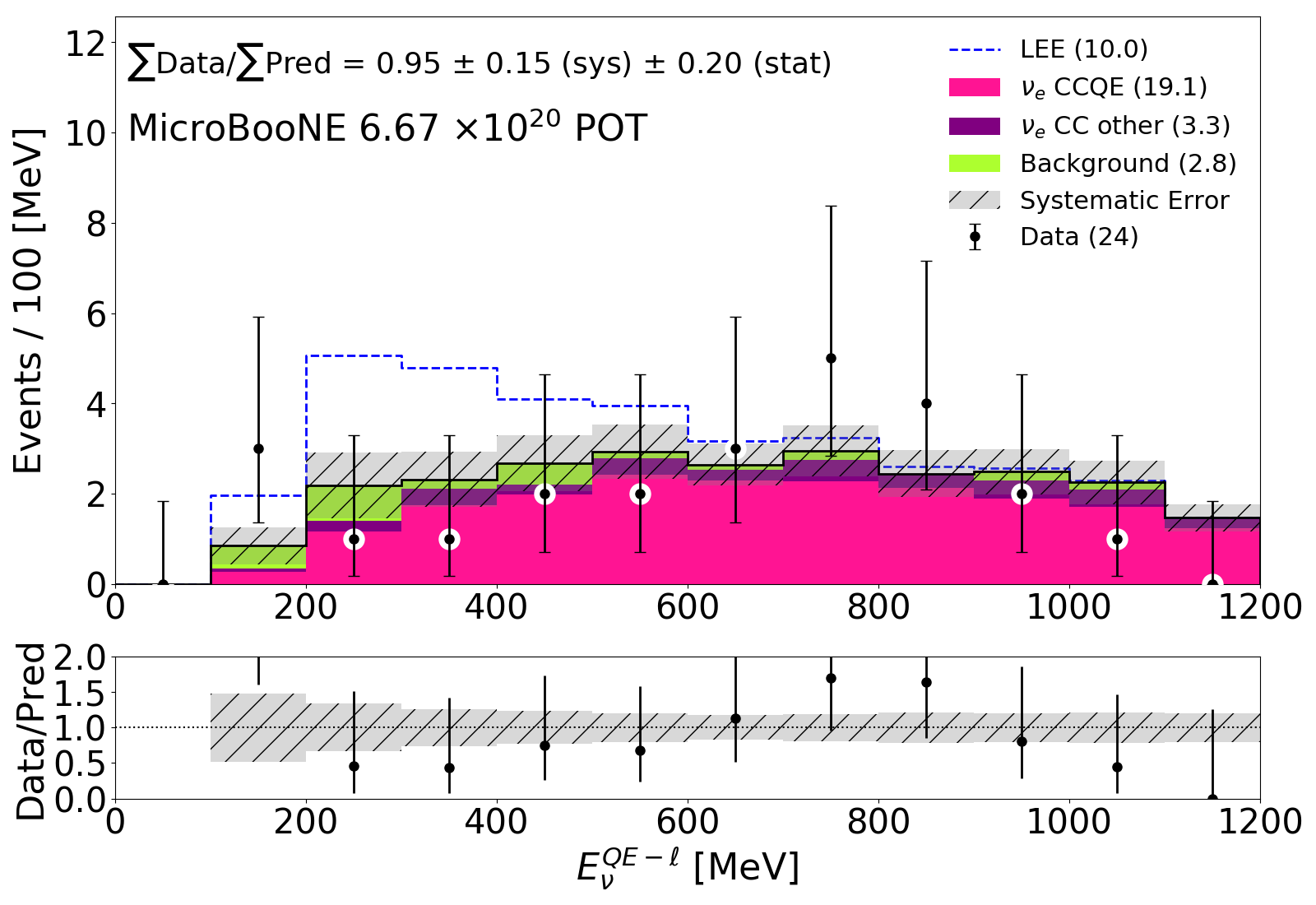
(d)

Figure 5.4: Comparison between data and unconstrained prediction in the $E_{e}$ (figure 5.4(a)), $E_{p}$ (figure 5.4(b)), $\theta_{e}$ (figure 5.4(c)), and $E_{\nu}^{QE-\ell}$ (figure 5.4(d)) distributions of the $1e1p$ sample.

5.1.1 Background Estimation

In table 5.1 we give a breakdown of the MC events in the “background” category of figures 5.3 and 5.4 by their interaction channel and event topology. The “off-vertex” label in this table refers to events for which the reconstructed neutrino vertex is further than 5 cm away from the true neutrino vertex. These events can happen when a cosmic muon track happens to cross a photon shower from a $\pi^{0}$ decay, or a muon decays to a Michel electron; in both cases, the muon is mistaken for a proton. Table 5.1 indicates that $\nu_{\mu}$ resonant $\pi^{0}$ events are the most common background interaction channel, followed by off-vertex events. One can also see that events with a $\pi^{0}$ in the final state are the dominant background topology.

There are not many MC events to inform the numbers reported in table 5.1. The tools developed for this analysis produce a highly pure $\nu_{e}$ CCQE sample, resulting in a low-statistics simulation sample for assessing the non-$\nu_{e}$ background to the $1e1p$ signal. This is apparent in the fluctuations of the background prediction in figures 5.3 and 5.4. In order to obtain a more robust prediction of this background, we have elected to leverage information on the energy distribution of non-$\nu_{e}$ background events at a loose BDT score cutoff of 0.7 and extrapolate this to our signal cutoff of 0.95. This is accomplished by fitting a parameterized Landau+linear probability density function (PDF) to the background energy distribution at the loose cutoff and scaling this prediction to the signal cutoff. As most of these backgrounds come from $\nu_{\mu}$ interactions, this is referred to as the $\nu_{\mu}$ background fit.

The Landau+linear shape is motivated empirically by the observation of a rise in the background rate toward the lowest energies ($\lesssim 500$ MeV) and a smaller rise toward the highest energies ($\gtrsim 800$ MeV), both for the loose BDT score cutoff and the signal cutoff, as shown by the blue points in figure 5.5. The Landau portion of the fit is additionally motivated by the observation that a majority of $\nu_{\mu}$ background events contain a $\pi^{0}$ in the final state, for which one of the decay photons is misinterpreted as an electron shower. The reconstructed neutrino energy of these events is governed predominately by the energy of this photon, which has a tail extending to higher energies caused by pions with high momentum in the lab frame. This tail is a characteristic feature of the Landau function. The output of the fit and resulting error are used in place of the raw prediction and statistical error for the $\nu_{\mu}$ backgrounds in this analysis. We note here that the simulated $\nu_{\mu}$ events with a $\pi^{0}$ in the final state are weighted according to the observation in our dedicated $\pi^{0}$ sample. The method for calculating these weights is described in Ref. [148].

The predicted background spectrum in each reconstructed neutrino energy bin $f(E_{i})$ is generated by integrating the Landau+linear PDF $p(E)$ within that bin. Specifically,

$$\begin{split}&p(E)=\exp\bigg{[}\frac{-(E^{\prime}+e^{-E^{\prime}})}{2}\bigg{]}+aE,\\ &E^{\prime}=(E-\mu)/\sigma,\\ &f(E_{i})=\int_{E_{i}-\delta E_{i}}^{E_{i}+\delta E_{i}}p(E)dE,\end{split}$$ (5.1)

where $\mu$ and $\sigma$ are the center and width of the Moyal approximation of the Landau function [202], $a$ is the linear slope parameter, $E_{i}$ is the center of the i’th energy bin, and $\delta E_{i}$ is half of the bin width. The Landau+linear fit is carried out using only shape information at a loose BDT score cutoff of 0.7. In order to get the overall normalization, we fit the BDT score distribution of the backgrounds to a linear PDF $\tilde{p}(x)$, which we can integrate to get the total expected number of background events $\tilde{f}(x)$ for a given BDT score cutoff $x$,

$$\tilde{p}(x)=mx+b~{}~{}~{}~{}\tilde{f}(x)=\int_{x}^{1}\tilde{p}(x)dx,$$ (5.2)

where $m$ and $b$ are the slope and bias parameters for the BDT score distribution, respectively. The resulting shape+normalization fit for the background distribution at the loose BDT cutoff of 0.7 and signal cutoff of 0.95 are shown in Fig. 5.5. One can see that the fit agrees with the raw MC prediction within statistical error in both cases and that the error on the fit is generally reduced compared to the simulation statistical error.

The errors on the fits in Fig. 5.5 are obtained by simulating pseudo-experiments according to the covariance matrix of the fit parameters. This is accomplished efficiently using Cholesky decomposition [203]. The overall normalization error on the background rate at a given BDT score cutoff is calculated using the error on the linear fit to the BDT score distribution of background events. For the Landau+linear fit, we generate a shape-only covariance matrix for the $\nu_{\mu}$ backgrounds in the nominal reconstructed neutrino energy bins. The overall normalization error has been added as a fully-correlated contribution to each bin of the shape-only $E_{\nu}$ covariance matrix. The uncorrelated uncertainty from the fit, given by the square root of the diagonal entries of the full (shape $\oplus$ normalization) covariance matrix, is indicated by the orange band in Fig. 5.5. This covariance matrix replaces the nominal statistical uncertainty on the simulated background, given by the quadrature sum of weights in each $E_{\nu}$ bin, which is indicated by the shaded blue band in Fig. 5.5.

The performance of the fit is evaluated on data by examining events slightly below the signal region, with a BDT score in the range $[0.7,0.95]$. These events are shown in Fig. 5.6. The raw MC prediction is given by the stacked histogram, while the prediction incorporating the $\nu_{\mu}$ background fit on top of the simulated $\nu_{e}$ prediction is given by the red line. The data agree well with both predictions, indicating the consistency of the fit method presented here with both the observed and MC-predicted background rate.

Interaction Channel	Predicted Rate
$\nu_{\mu}$ resonant $\pi^{0}$	1.26
$\nu_{\mu}$ resonant $\pi^{\pm}$	0.21
$\nu_{\mu}$ CCQE	0.14
$\nu_{\mu}$ other	0.19
Off-vertex	0.93
Event Topology	Predicted Rate
$1\mu N\pi^{0}$	0.57
$0\mu N\pi^{0}$	1.09
$1\mu 1p$	0.14
Off-vertex	0.93

Table 5.1: Breakdown of MC events in the “background” category of figures 5.3 and 5.4 over the range $200<E_{\nu}<1200$ MeV. The events are partitioned both by the interaction channel and the event topology.

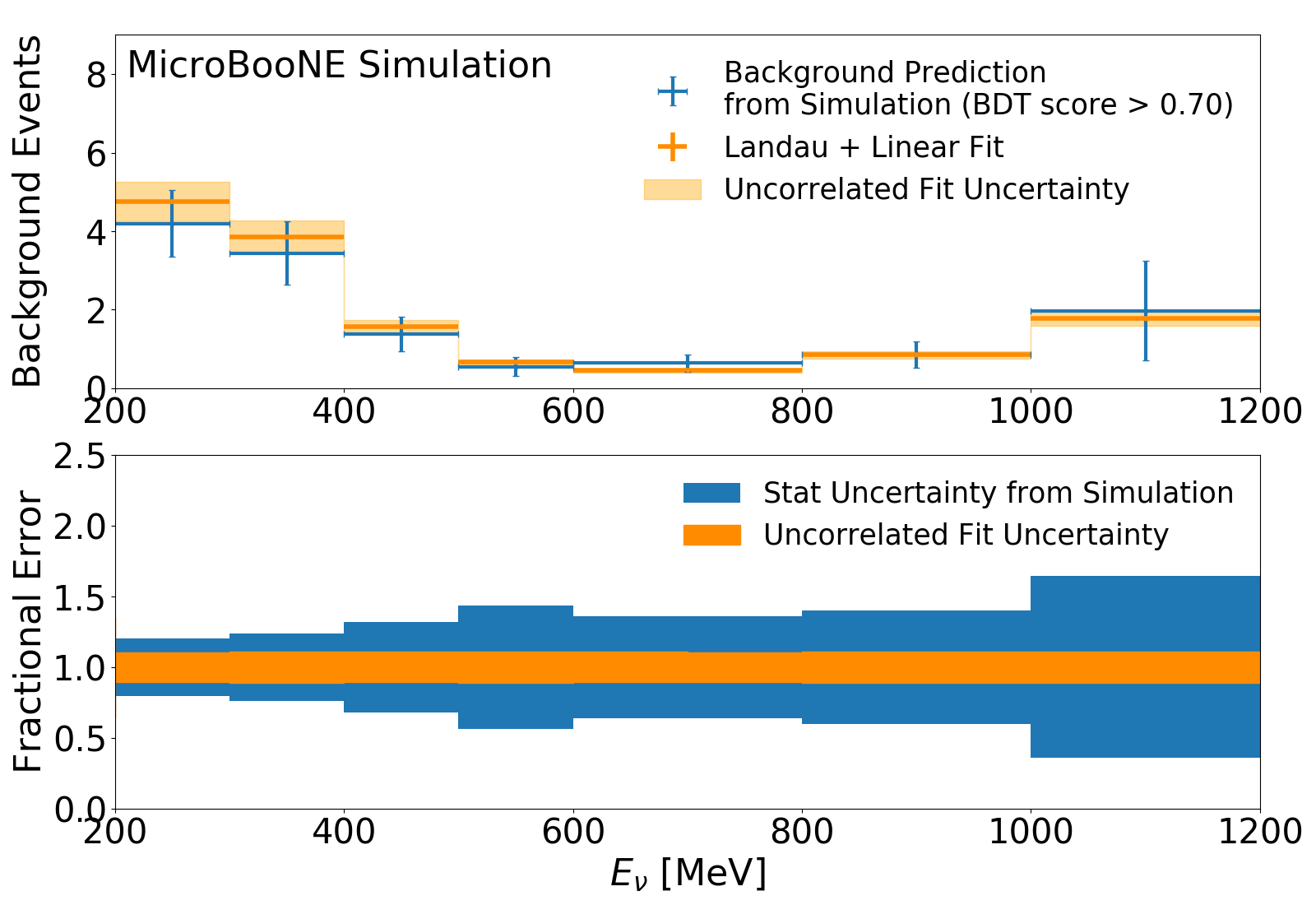
(a)

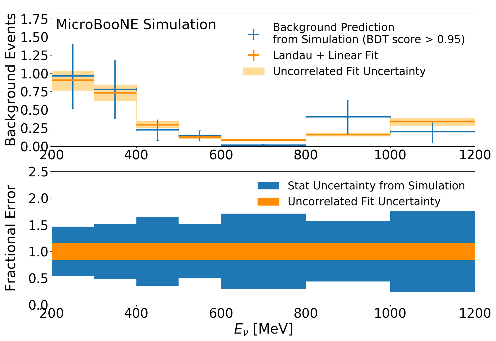
(b)

Figure 5.5: The fit to the $\nu_{\mu}$ background distribution to the $1e1p$ analysis. The shape fit is performed at a loose BDT score cutoff of 0.7 (figure 5.5(a)) and scaled to the signal cutoff of 0.95 (figure 5.5(b)). Blue points represent the prediction from the simulation, with error bars representing the Gaussian approximation of the statistical error (quadrature sum of event weights). The orange line and corresponding shaded region represent prediction and uncertainty, respectively, coming from the Landau+linear fit.

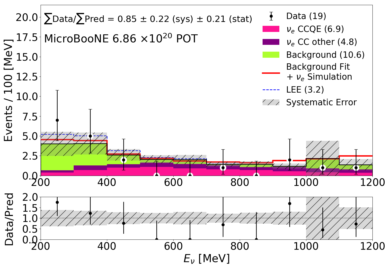
Figure 5.6: The data and MC prediction for events with a $1e1p$ BDT score inside $[0.7,0.95]$. Good agreement is observed between data and prediction. The prediction incorporating the Landau+linear background fit is shown by the red line.

5.1.2 Evaluation of Systematic Uncertainties

There are five main sources of systematic uncertainty in this analysis, related to the beam flux, neutrino-nucleus cross section modeling, hadron re-interaction modeling, detector simulation, and finite statistics in the MC-based prediction. These are handled within a covariance matrix formalism. For each binned distribution, the diagonal entries of the covariance matrix contain the variance in each bin, while the off-diagonal entries contain the covariance between different bins. Thus, the covariance matrix is also symmetric. The use of a covariance matrix is essential for encoding correlations between binned distributions of selected events in the $1e1p$ and $1\mu 1p$ samples, which is relevant for the constraint procedure described in section 5.1.3. The total covariance matrix for a given distribution is simply the element-wise sum of the covariance matrices for each source of systematic uncertainty. A few definitions will be helpful for our discussion here; given a covariance matrix $M_{ij}$ and binned prediction $N_{i}$, the fractional covariance matrix is given by $F_{ij}\equiv M_{ij}/(N_{i}N_{j})$ and the correlation matrix is given by $\rho_{ij}\equiv M_{ij}/\sqrt{M_{ii}M_{ij}}$. The correlation matrix is meant to capture the degree of correlation between two bins normalized within the range $[-1,1]$, where diagonal entries are 1 by construction.

The flux, cross section, and re-interaction uncertainties are evaluated using a reweighting method, in which event weights are modified according to tunable parameters. Variations in the distributions of reconstructed variables are used to determine the associated covariance matrix. The detector systematic covariance matrix is evaluated using a dedicated set of simulation samples that each alter the detector response in a different way. These alterations to the detector response are derived using cosmic muon data; the full procedure is described in detail in Ref. [204].

Flux uncertainties are related to hadron production in the target, secondary hadron interactions, and focusing efficiency of the BNB magnetic horn. Neutrino events are reweighted according to the species and momentum of the parent meson [14, 205]. The largest flux uncertainty comes from $\pi^{+}$ production in the target. The flux uncertainties are also highly correlated between the $1e1p$ and $1\mu 1p$ samples, as they both come predominately from the same meson decay chain, $\pi^{+}\to\nu_{\mu}(\mu^{+}\to e^{+}\nu_{e}\overline{\nu}_{\mu})$.

The cross section covariance matrix is calculated using both interaction-specific reweightable parameters and FSI-related reweightable parameters in GENIE v3.00.06. Thus, each MC event is reweighted according to its interaction channel and any final state particles which underwent FSI. The full suite of reweightable parameters is described in Ref. [180]. We also evaluate uncertainties related to the difference between the $\nu_{e}$ CCQE and $\nu_{\mu}$ CCQE cross sections [206]. The largest cross section uncertainties come from CCQE-related parameters, which is expected given our signal definition, and FSI-related parameters. FSI uncertainties are especially important in this analysis, as FSI can cause $\nu_{e}$ CCQE events to deviate from two-body scattering kinematics and also cause non-$\nu_{e}$ CCQE events to look more consistent with two-body scattering. Both CCQE-related and FSI-related effects impact the $1e1p$ and $1\mu 1p$ samples similarly and thus are at least partially addressed by the constraint procedure in section 5.1.3.

Hadron re-interaction uncertainties describe the scattering of final state protons and $\pi^{\pm}$ off of argon nuclei. The covariance matrix is calculated by reweighting events according to Geant4 truth-level information about the hadron trajectory [207]. These uncertainties are a small effect in this analysis.

The detector systematic covariance matrix is calculated using a set of dedicated simulation samples that vary certain aspects of the detector response. These include the amplitude and width of TPC signals as a function of the $x$ and $(y,z)$ positions as well the directions $\theta_{XZ}$ and $\theta_{YZ}$ of the charged particle; the electron-ion recombination rate; the electric field map in the TPC; and the light yield, attenuation, and Rayleigh scattering length. As these samples are computationally expensive to generate, we are not left with many MC events with which to construct a covariance matrix. Thus, we rely on kernel density estimation [208, 209] to smooth the predictions in each detector variation sample. This procedure does not work for the $\nu_{\mu}$ backgrounds to the $1e1p$ analysis since we are especially starved for MC statistics here, as discussed in section 5.1.1. We instead assign a conservative uncorrelated 20% fractional detector systematic uncertainty on these events, based on the extent of differences in the total rate of selected background events in the detector variation samples.

The variance due to finite MC statistics is simply given by the quadrature sum of event weights in each bin. These uncertainties are uncorrelated and give a diagonal covariance matrix. The exception is finite MC statistics uncertainties on the $\nu_{\mu}$ backgrounds in the $1e1p$ analysis, which are calculated using the procedure described in section 5.1.1.

Finally, we note that to evaluate the reweightable systematic uncertainties on the $\nu_{\mu}$ backgrounds to the $1e1p$ analysis, we use the selected MC events to calculate a fractional covariance matrix, which is then scaled by the parameterized background prediction derived in section 5.1.1. When performing the constraint in section 5.1.3, we do not consider off-diagonal systematic uncertainties between $\nu_{\mu}$ backgrounds in the $1e1p$ sample and bins in the $1\mu 1p$ sample, as it is not straightforward to compute this correlation.

The fractional uncertainty in each bin of the $E_{\nu}^{\rm range}$ distribution in the $1e1p$ and $1\mu 1p$ samples is shown in figure 5.7. These correspond to the square root of the diagonal entries of the total systematic covariance matrix calculated from all sources described above, divided by the predicted event rate in each bin. In the $1e1p$ sample, flux, cross section, and detector uncertainties dominate at low energies while detector uncertainties dominate at high energies. The joint $1e1p$ and $1\mu 1p$ covariance and correlation matrices are shown in figure 5.8. The large off-block-diagonal correlations between the $1e1p$ and $1\mu 1p$ samples will be exploited in section 5.1.3.

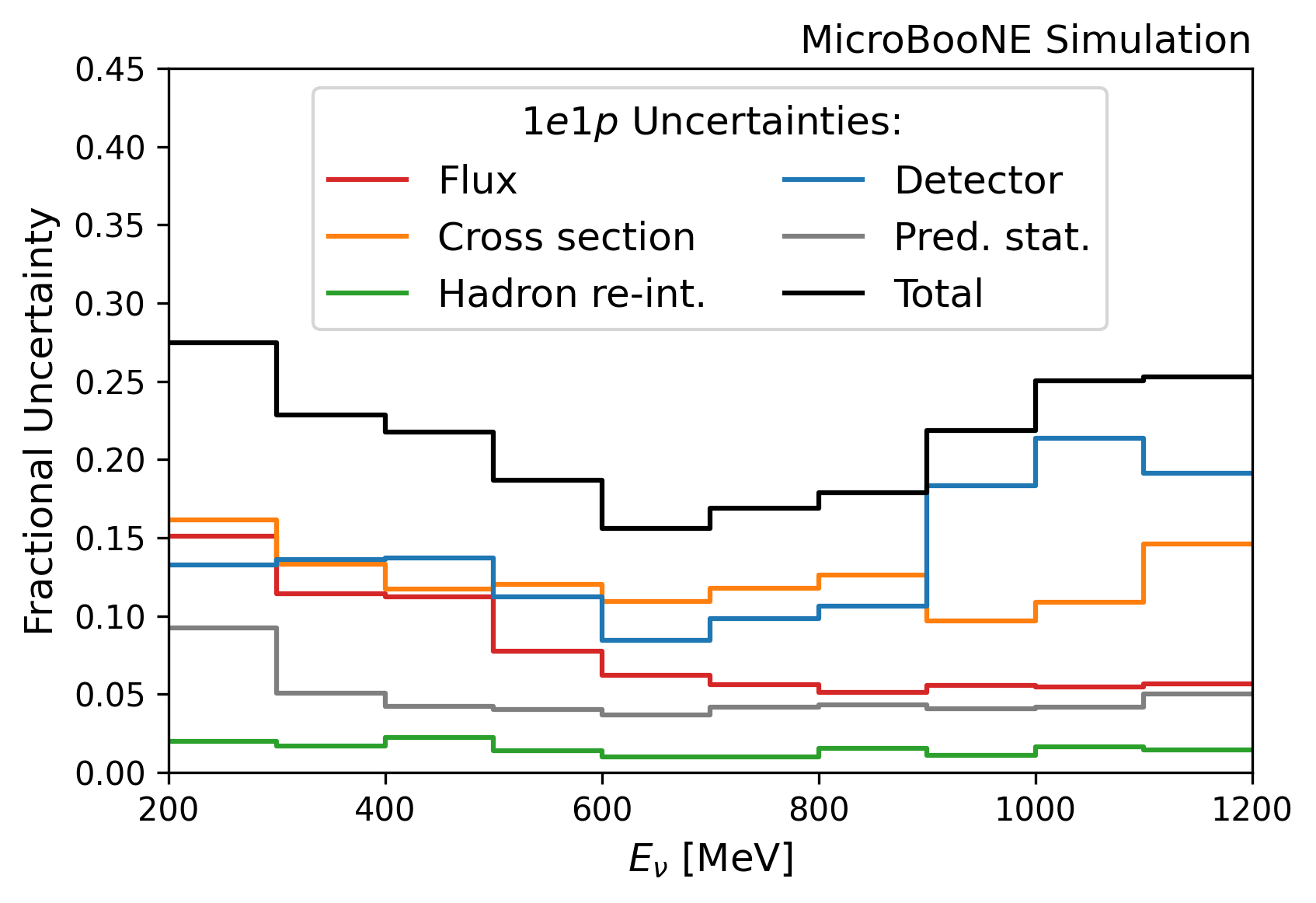
(a)

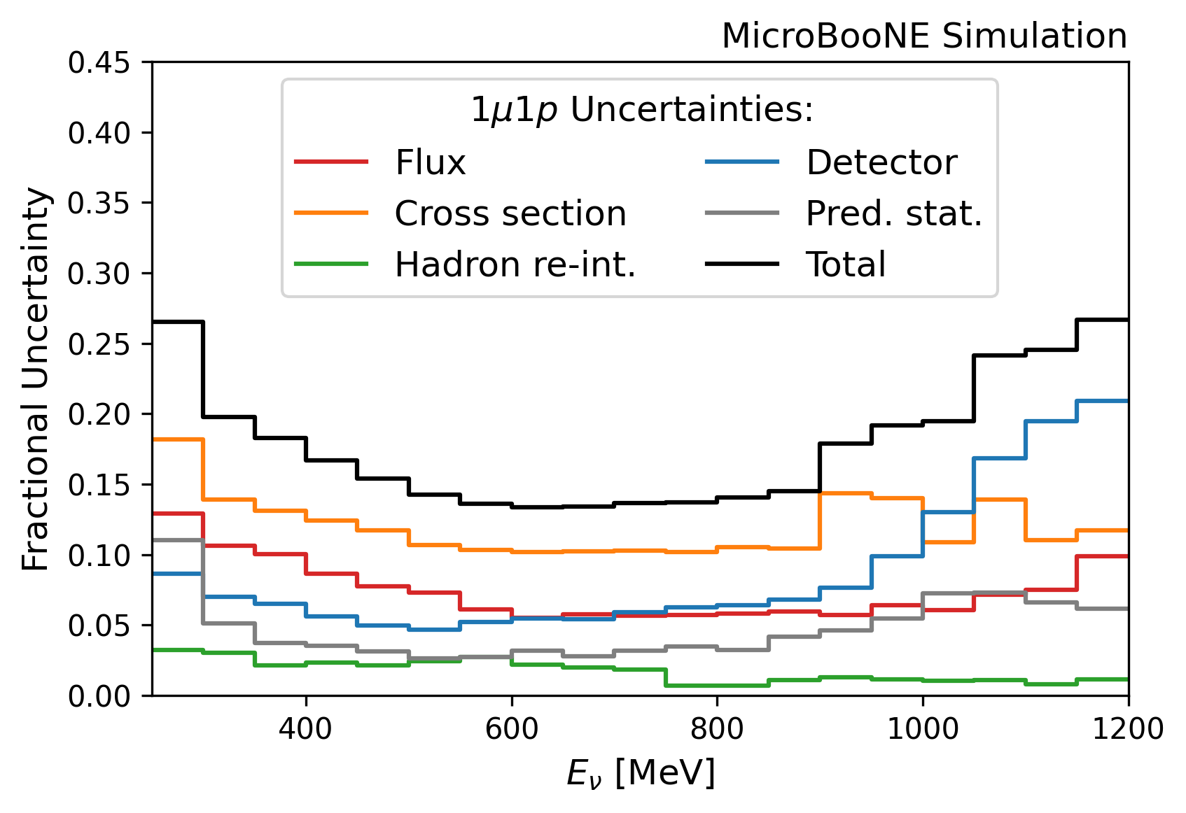
(b)

Figure 5.7: The uncertainty in each bin of the $E_{\nu}^{\rm range}$ distribution of the $1e1p$ (figure 5.7(a)) and $1\mu 1p$ (figure 5.7(b)) samples.

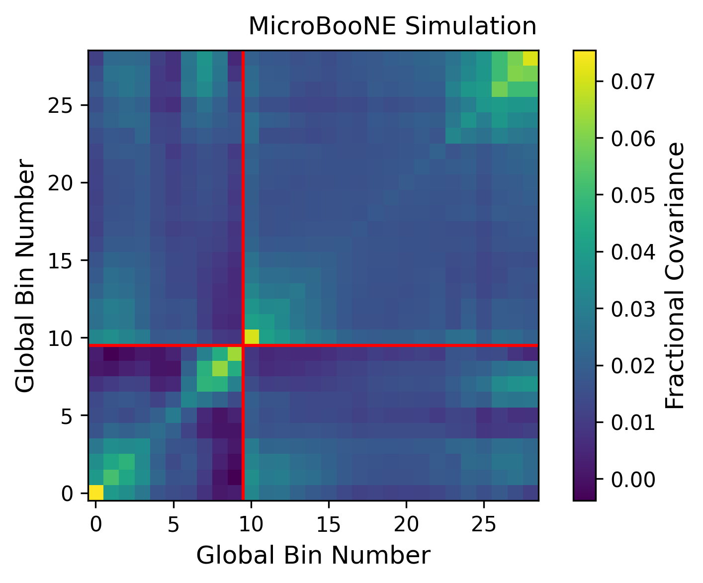
(a)

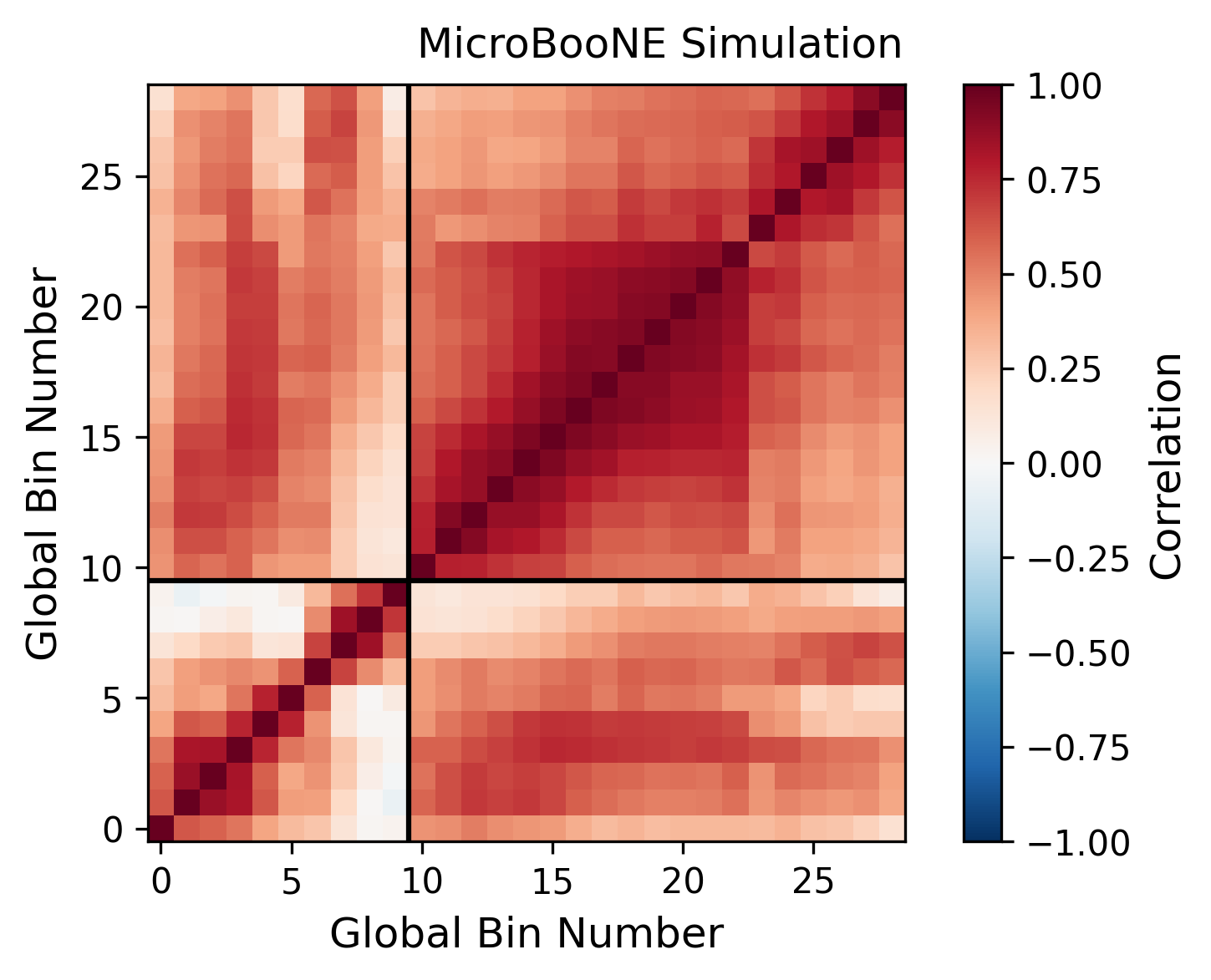
(b)

Figure 5.8: The joint covariance (figure 5.8(a)) and correlation (figure 5.8(b)) matrices for the $E_{\nu}^{\rm range}$ distribution of the $1e1p$ and $1\mu 1p$ samples.

5.1.3 Constraint from the $1\mu 1p$ Sample

As alluded to thus far, we use the observation in the $1\mu 1p$ control sample to constrain the prediction and uncertainties in the $1e1p$ signal sample. We rely on the conditional covariance method, which has also been used by the MiniBooNE collaboration [76]. We perform the constraint in the $E_{\nu}^{\rm range}$ distribution of each sample. Let us represent the joint covariance matrix between both samples shown in figure 5.8(a) as

$$M=\begin{pmatrix}M^{ee}&M^{e\mu}\\ M^{\mu e}&M^{\mu\mu}\\ \end{pmatrix}.$$ (5.3)

Given a measurement $d_{\mu}$ and prediction $\mu_{\mu}$ in the $1\mu 1p$ channel, the constrained prediction $\mu_{e,{\rm const}}$ and covariance matrix $M^{ee,{\rm const}}$ are given by [170]

$$\begin{split}&\mu_{e,{\rm const}}=\mu_{e}+M^{e\mu}\cdot(M^{\mu\mu})^{-1}\cdot(d_{\mu}-\mu_{\mu}),\\ &M^{ee,{\rm const}}=M^{ee}-M^{e\mu}\cdot(M^{\mu\mu})^{-1}\cdot M^{\mu e},\end{split}$$ (5.4)

where $\mu_{e}$ is the nominal prediction in the $1e1p$ channel before the constraint.

Figure 5.9 shows the comparison between data and prediction in the $1\mu 1p$ $E_{\nu}^{\rm range}$ distribution. This observation is used as input to the constraint procedure in equation 5.4. The diagonal uncertainties in the $1e1p$ $E_{\nu}^{\rm range}$ distribution are reduced by up to a factor of $\sim 2$ across most bins, as shown in figure 5.10. In figure 5.11 we compare observed data to the final constrained prediction and uncertainties in the $1e1p$ $E_{\nu}^{\rm range}$ distribution. As can be seen, the constraint procedure slightly increases the $1e1p$ prediction at lower $E_{\nu}^{\rm range}$ values, though this is not a large effect. The result shown in figure 5.11 forms the basis of the statistical tests discussed in section 5.2.

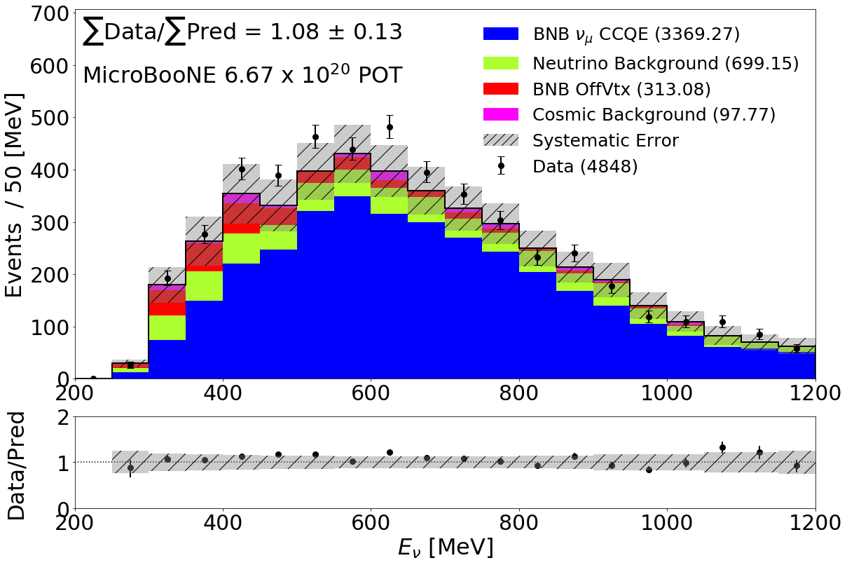
Figure 5.9: The $E_{\nu}^{\rm range}$ distribution in the $1\mu 1p$ channel, comparing data to the MC prediction.

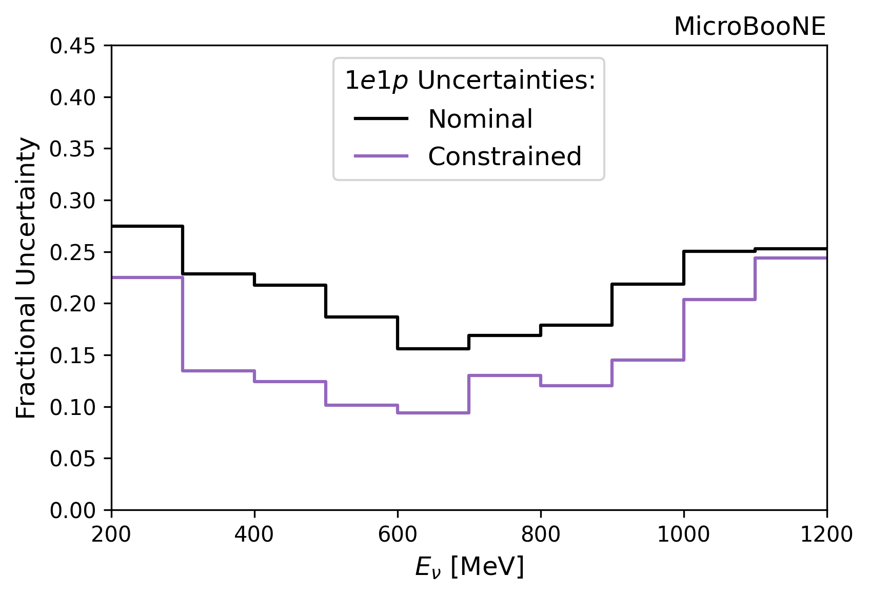
Figure 5.10: Fractional systematic uncertainty in the $1e1p$ $E_{\nu}^{\rm range}$ distribution before and after the $1\mu 1p$ constraint.

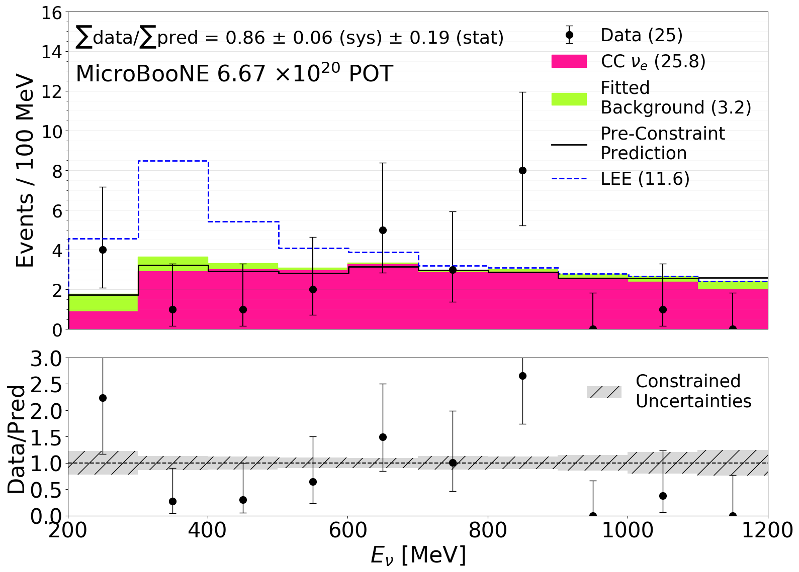
Figure 5.11: Comparison between data and prediction in the $1e1p$ $E_{\nu}^{\rm range}$ distribution after applying the $1\mu 1p$ constraint procedure.

5.1.4 Blinded Analysis Approach

Here we briefly cover the blind analysis procedure and related cross-checks performed before examining data in the $1e1p$ signal sample. The main strategy here was to use a sequential unblinding approach. Data were first examined for events with a low BDT score ($<0.7$) or a high reconstructed neutrino energy ($>700$ MeV). Next, we examined data with a medium BDT score (within $[0.7,0.95]$) or medium energy ($500-700$ MeV). Only after establishing good agreement between data and prediction in all of these samples were potential signal events first examined, where signal events are defined to have a $1e1p$ BDT score greater than 0.95 and reconstructed neutrino energy below 500 MeV. This sequence was chosen because sensitivity to the eLEE model is minimized at lower BDT scores and higher neutrino energies. Moving on to each subsequent stage required signoff from the entire MicroBooNE collaboration. Figure 5.12 shows the comparison between data and prediction in the $1e1p$ BDT ensemble average score distribution for this “medium BDT score” sample. Figure 5.6 is another example of one of the “medium BDT score” plots.

We also explored a sample that made a number of cuts on kinematic variables in order to mimic the $1e1p$ BDT ensemble cut. As humans are poorer optimizes than BDTs, this sample contained a much larger rate of $\nu_{\mu}$ background events compared to the official signal selection. Good agreement between data and prediction was observed across all variables explored within this sample, thus giving confidence in the MC description of backgrounds to the $1e1p$ signal sample.

Finally, before any $\nu_{e}$ analysis was able to look at data in their signal sample, we each had to pass a series of fake data tests. In these tests, five different data-like MC samples were generated with various unknown alterations to the nominal MC. These included, for example, the presence of a large $\nu_{e}$ eLEE signal and alterations to underlying cross section models. All three $\nu_{e}$ analyses ran through the statistical results presented in section 5.2 for each fake data sample. In all cases, the statistical conclusions determined from each fake dataset were consistent with the truth-level injected events. At this point, the $\nu_{e}$ analyses (including the two-body CCQE analysis) were ready to move on to the real signal dataset.

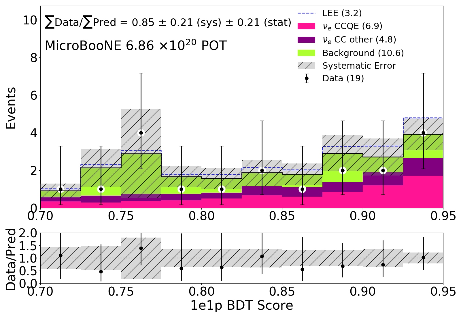
Figure 5.12: Comparison between data and prediction in the $1e1p$ BDT ensemble average score distribution within the range $[0.7,0.95]$.

5.2 Statistical Interpretation

We perform three different statistical tests of the eLEE model: a $\chi^{2}$ goodness-of-fit test, a $\Delta\chi^{2}$ two-hypothesis test, and a signal strength scaling test. We use the combined Neyman-Pearson (CNP) chi-square test statistic [210],

$$\chi^{2}_{\rm CNP}=(\vec{d}-\vec{\mu})^{T}(M^{\rm stat}_{\rm CNP}+M^{\rm sys})^{-1}(\vec{d}-\vec{\mu}),$$ (5.5)

where $\vec{d}$ and $\vec{\mu}$ are the observation and prediction for a particular distribution, $M^{\rm sys}$ is the systematic covariance matrix described in section 5.1.2, and

$$(M^{\rm stat}_{\rm CNP})_{ij}\equiv\frac{3\delta_{ij}}{\frac{1}{d_{i}}+\frac{2}{\mu_{i}}}.$$ (5.6)

This formulation of the statistical error is meant to more closely approximate the Poisson likelihood, which is important given the low-statistics nature of the $1e1p$ analysis. Unlike the Poisson likelihood, the CNP chi-square test statistic is compatible with the covariance matrix formalism developed for our systematic uncertainty treatment.

All statistical tests use the constrained $1e1p$ prediction and uncertainties shown in figure 5.11 when comparing to the 25 observed data events. We define two distinct hypotheses which we will refer to in the following discussion: $H_{0}$, the prediction without the eLEE model, considering only intrinsic $\nu_{e}$ events and non-$\nu_{e}$ backgrounds (i.e. the stacked histogram in figure 5.11); and $H_{1}$, the prediction including the eLEE model (i.e. the dashed blue line in figure 5.11). Throughout this section, we report probabilities, or $p$-values, calculated using the following frequentist method. To test the distribution of a specific variable under a given hypothesis, $10^{5}$ pseudo-experiments are generated by sampling the multivariate distribution defined by the prediction and covariance matrix of the hypothesis. This gives a predicted rate in each bin of the distribution; we use this to sample from a Poisson distribution to get an integer number of “observed” events in each bin. We calculate the desired test statistic for each pseudo-experiment to build up the probability distribution of that test statistic, which incorporates both systematic and statistical uncertainties. Then, we can compare the observed value of the test statistic in the real dataset to the calculated probability distribution to determine the probability of observing a more extreme value–this defines the $p$-value.

5.2.1 Goodness of Fit

For the first test, we evaluate the goodness of fit in the $1e1p$ sample for $H_{0}$ and $H_{1}$ using the $\chi^{2}_{\rm CNP}$ test statistic. This is done both before and after the $1\mu 1p$ constraint. We also consider the goodness-of-fit in both the full analysis range, $200<E_{\nu}^{\rm range}\;[{\rm MeV}]<1200$, and the low energy region $200<E_{\nu}^{\rm range}\;[{\rm MeV}]<500$, where the eLEE model prediction is highest. Table 5.2 shows the $\chi^{2}_{\rm CNP}$ per degree-of-freedom (DOF) for each of these scenarios, as well as the corresponding $p$-values calculated via the frequentist method described above.

The first thing to note there is significant tension with $H_{1}$, especially after the $1\mu 1p$ constraint, as indicated by the low $p$-values. This is true both over the full analysis energy range and in the low energy range. After the constraint, there is greater than $3\sigma$ tension between $H_{1}$ and the observed data across the full energy range.

There is also disagreement between $H_{0}$ and the observed data, though not to the same level as the $H_{1}$ case. Over the full analysis energy range, the $p$-values in table 5.2 indicate $2.1\sigma$ ($2.4\sigma$) tension between $H_{0}$ and the data before (after) the $1\mu 1p$ constraint. This seems to come from two sources: the deficit in data compared to prediction below $500$ MeV in figure 5.11, and the excess in the 800-900 MeV bin in figure 5.11. The first of these is possibly a real effect–similar low-energy deficits are observed by all three $\nu_{e}$ analyses [116]. It is also observed in the $E_{\nu}^{QE-\ell}$ distribution in figure 5.4(d) and is therefore not likely to be related to proton misreconstruction. Our Michel electron sample covered in section 4.4.3 indicates robust modeling of low-energy electron showers, so this is also unlikely to be the culprit. The excess in the 800-900 MeV bin, however, appears to be a statistical fluctuation. The other variables examined in this analysis all show good agreement between data and MC and do not have similar narrow excesses. For instance, the $E_{e}$, $E_{p}$, $\theta_{e}$, and $E_{\nu}^{QE-\ell}$ distributions in figure 5.4 have a $\chi^{2}_{\rm CNP}$/DOF ($p$-value) of 10.68/10 (0.42), 5.77/10 (0.80), 10.19/10 (0.48), and 11.46/10 (0.52), respectively. The $\chi^{2}_{\rm CNP}$/DOF and $p$-value of all 36 variables examined in this analysis are reported in the Supplemental Material of Ref. [148].

Nominal Predictions
Range	$H_{0}$		$H_{1}$
	$\chi^{2}_{\text{CNP}}/\text{DOF}$	$p$-value	$\chi^{2}_{\text{CNP}}/\text{DOF}$	$p$-value
200–500 MeV	6.06/3	0.138	8.30/3	0.053
200–1200 MeV	23.02/10	0.024	25.37/10	0.014
Constrained Predictions
Range	$H_{0}$		$H_{1}$
	$\chi^{2}_{\text{CNP}}/\text{DOF}$	$p$-value	$\chi^{2}_{\text{CNP}}/\text{DOF}$	$p$-value
200–500 MeV	7.91/3	0.075	17.3/3	0.002
200–1200 MeV	25.28/10	0.014	36.35/10	$5.0\times 10^{-4}$

Table 5.2: Results from goodness-of-fit tests comparing observed $1e1p$ data to the $H_{0}$ and $H_{1}$ predictions, reported via the $\chi^{2}_{\text{CNP}}$ test statistic and the frequentist $p$-value. The top half of the table considers the nominal prediction and uncertainties before the $1\mu 1p$ constraint described in section 5.1.3, while the bottom half considers the post-constraint prediction and uncertainties.

5.2.2 Two Hypothesis Test

The next test we perform is a two-hypothesis $\Delta\chi^{2}$ test between $H_{0}$ and $H_{1}$. Specifically, we use the test statistic

$$\Delta\chi^{2}=\chi^{2}_{{\rm CNP},H_{0}}-\chi^{2}_{{\rm CNP},H_{1}}.$$ (5.7)

Thus, a positive (negative) value indicates better agreement with $H_{1}$ ($H_{0}$). For this test, we consider the post-$1\mu 1p$-constraint prediction and errors for the $1e1p$ sample. Figure 5.13 shows the distribution of this test statistic under both hypotheses, generated using the frequentist method described above. As expected, the $H_{0}$ distribution peaks below zero while the $H_{1}$ distribution peaks above zero. These distributions can be used to determine the one-sided exclusion sensitivity of each hypothesis in the two-body CCQE analysis. If we denote the median $\Delta\chi^{2}$ value under $H_{1}$ as $(\Delta\chi^{2})_{H_{1}}^{\rm med}$, the probability of $H_{0}$ generating a larger $\Delta\chi^{2}$ than $(\Delta\chi^{2})_{H_{1}}^{\rm med}$ is 0.003. This corresponds to an $H_{0}$ exclusion sensitivity of $2.7\sigma$. Conversely, if we define $(\Delta\chi^{2})_{H_{0}}^{\rm med}$ in an analogous way, the probability of $H_{1}$ generating a smaller $\Delta\chi^{2}$ than $(\Delta\chi^{2})_{H_{0}}^{\rm med}$ is 0.017, corresponding to an $H_{1}$ exclusion sensitivity of $2.1\sigma$.

As shown in figure 5.13, the observed data result in a test statistic of $\Delta\chi^{2}=-11.08$. The probability of observing a smaller $\Delta\chi^{2}$ under $H_{0}$ and $H_{1}$ is 0.020 and $1.6\times 10^{-4}$, respectively, corresponding to a Gaussian significance of $2.1\sigma$ and $3.6\sigma$. Thus, the data exhibits mild tension with $H_{0}$ and significant tension with $H_{1}$. A similar conclusion was reached for the goodness-of-fit test; the tension with $H_{0}$ likely comes from the same sources discussed in section 5.2.1. Due to the fact that non-negligible tension is observed with respect to both hypotheses, we report our exclusion significance for $H_{1}$ using the CL_s method [211, 212]. The CL_s test statistic is defined as

$${\rm CL}_{s}=\frac{p_{H_{1}}}{p_{H_{0}}},$$ (5.8)

where ${\rm CL}_{s}=0.008$ for our observed data. Using this method, we reject $H_{1}$ in favor of $H_{0}$ with a Gaussian significance of $2.4\sigma$.

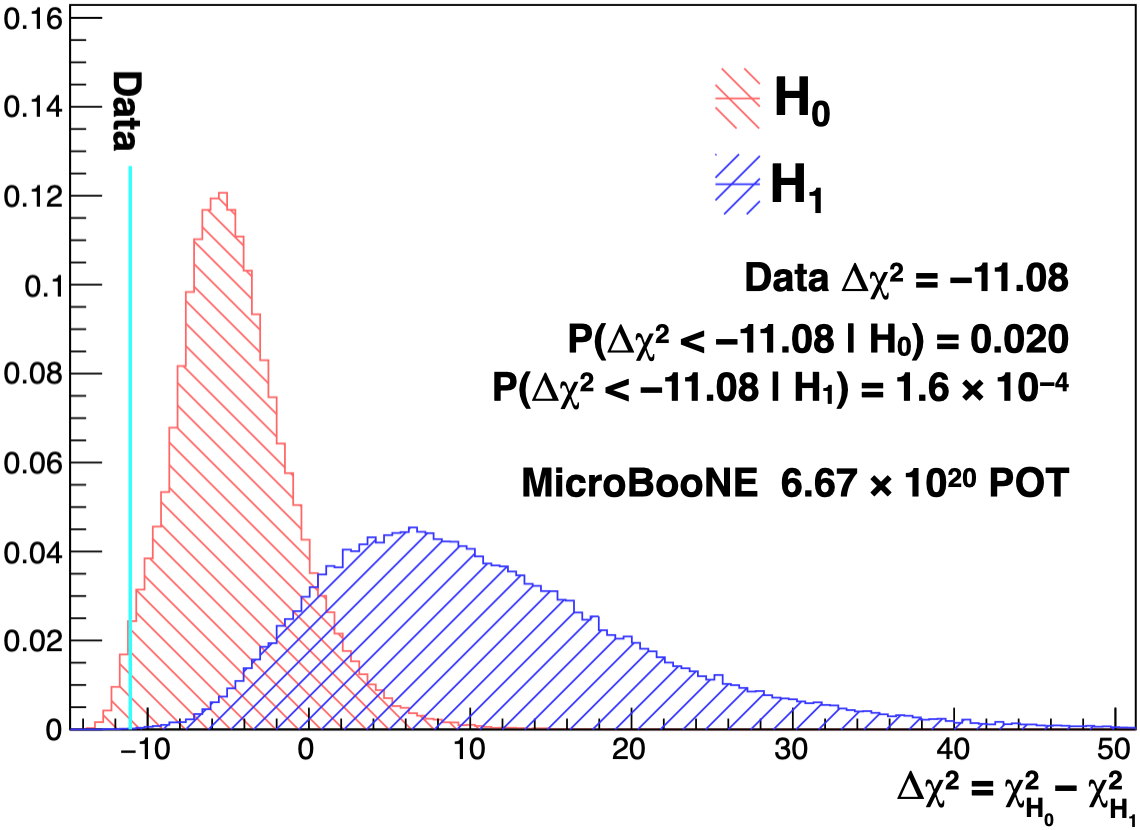
Figure 5.13: Distributions of the $\Delta\chi^{2}$ test statistic defined in equation 5.7 for $H_{0}$ (red) and $H_{1}$ (blue), calculated by generating $10^{5}$ pseudo-experiments under each hypothesis. The $\Delta\chi^{2}$ value of the data is also shown.

5.2.3 Signal Strength Scaling Test

The final statistical test we perform on our $1e1p$ dataset is a one-parameter signal strength scaling test. Specifically, we multiply by the eLEE weights in figure 4.1(b) by an overall normalization factor $x_{\rm LEE}$ which can vary within $[0,\infty]$. In this construction, $x_{\rm LEE}=0$ corresponds to $H_{0}$ and $x_{\rm LEE}=1$ corresponds to $H_{1}$. We can use the Feldman-Cousins procedure [25] along with the test statistic

$$\Delta\chi^{2}(x_{\rm LEE})=\chi^{2}_{\rm CNP}(x_{\rm LEE})-\min_{x_{\rm LEE}\in[0,\infty]}\{\chi^{2}_{\rm CNP}(x_{\rm LEE})\}$$ (5.9)

to determine confidence intervals on $x_{\rm LEE}$. We can use the Asimov dataset, in which the observation is exactly the predicted value in each bin, to determine the sensitivity to each hypothesis in this test. Under $H_{0}$, the expected upper bound on $x_{\rm LEE}$ at the 90% ($2\sigma$) confidence level is 0.75 (0.98). Under $H_{1}$, the expected confidence interval at the $1\sigma$ ($2\sigma$) confidence level is $[0.53,1.66]$ ($[0.28,2.67]$), and the expected sensitivity to rule out $x_{\rm LEE}=0$ is $2.8\sigma$.

Figure 5.14 shows the confidence intervals on $x_{\rm LEE}$ derived from the observed data. The best-fit value is $x_{\rm LEE}=0$, which is expected given the deficit in data at the lowest neutrino energies where the eLEE model weights are the largest. The 90% ($2\sigma$) upper bound on $x_{\rm LEE}$ is 0.25 (0.38). These upper bounds are stronger than the expected confidence intervals under $H_{0}$, which is mainly due to the aforementioned deficit at low neutrino energies.

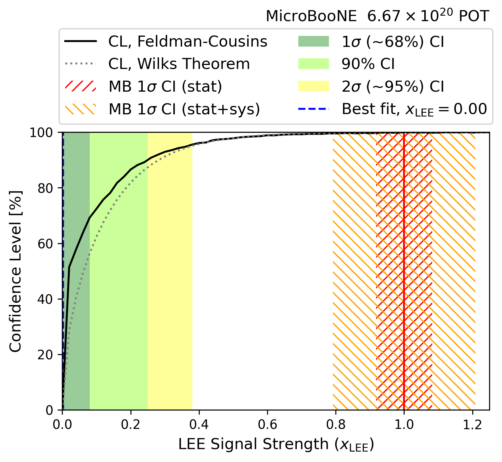
Figure 5.14: Confidence intervals on $x_{\rm LEE}$ calculating using the Feldman-Cousins procedure. The solid and dotted lines indicate the confidence level with which a given $x_{\rm LEE}$ is disfavored, calculated using the Feldman-Cousins method [25] and Wilks theorem [26], respectively. The MiniBooNE statistical and systematic errors are shown as a band around $x_{\rm LEE}=1$.

5.3 Discussion and Outlook

The observation in the $1e1p$ signal channel of the two-body CCQE analysis is inconsistent with a MiniBooNE-like excess of $\nu_{e}$ CCQE interactions. Under a two-hypothesis test, we rule out the nominal eLEE model ($H_{1}$) at the $2.4\sigma$ using the CL_s method. We can set an upper bound on the signal strength scaling parameter $x_{\rm LEE}$ of 0.38 at the $2\sigma$ level.

This is consistent with the results from all three MicroBooNE $\nu_{e}$ analyses [116]. As shown in figure 5.15(a), three of the four signal channels from the three $\nu_{e}$ analyses observe a deficit of selected events at the lowest neutrino energies, where the eLEE model is supposed to peak. The exception is the $1e0p0\pi$ channel from the MiniBooNE-like sample; however, this is the least sensitive of the four channels, as it is dominated by non-$\nu_{e}$ backgrounds. Figure 5.15(b) shows the results from the signal strength scaling test in all four channels. With the exception of the $1e0p0\pi$ channel, all analyses rule out $x_{\rm LEE}=1$ at greater than the $2\sigma$ confidence level. The most sensitive analyses observe an upper bound $x_{\rm LEE}\lesssim 0.5$ at the $2\sigma$ confidence level.

The first MicroBooNE results also included a search for $\Delta\to N\gamma$ decays as an explanation for the MiniBooNE excess. The analysis did not observe an excess of $\Delta\to N\gamma$ candidate events and ruled out the required enhancement to explain the MiniBooNE anomaly at the 95% confidence level. The full details of this analysis can be found in Ref. [80].

Thus, the MicroBooNE results disfavor both an enhancement of $\nu_{e}$ CC interactions and $\Delta\to N\gamma$ decays as the sole explanation of the MiniBooNE excess. Potential explanations of the MiniBooNE anomaly must now remain consistent with these MicroBooNE results. One promising avenue involves dark sector models which produce a photon or $e^{+}e^{-}$ pair in the MiniBooNE detector. Such event signatures have not yet been explored by MicroBooNE, though this work is in progress. Crefch:neutrissimos explores a photon-based explanation of MiniBooNE, involving the decay of a heavy neutral lepton to a single photon via a transition magnetic moment. The theoretical and experimental neutrino physics communities are actively working to develop innovative models to explain the MiniBooNE LEE and equally innovative measurements to test those models.

The following subsections close with two projects I co-led with various collaborators to follow up on the state of the MiniBooNE excess after the MicroBooNE results. The first examines the $3+1$ model simultaneously in MiniBooNE and MicroBooNE [102]. The second explores the implications of a $\overline{\nu}_{e}$-based MiniBooNE LEE for the MicroBooNE results [201].

(a)

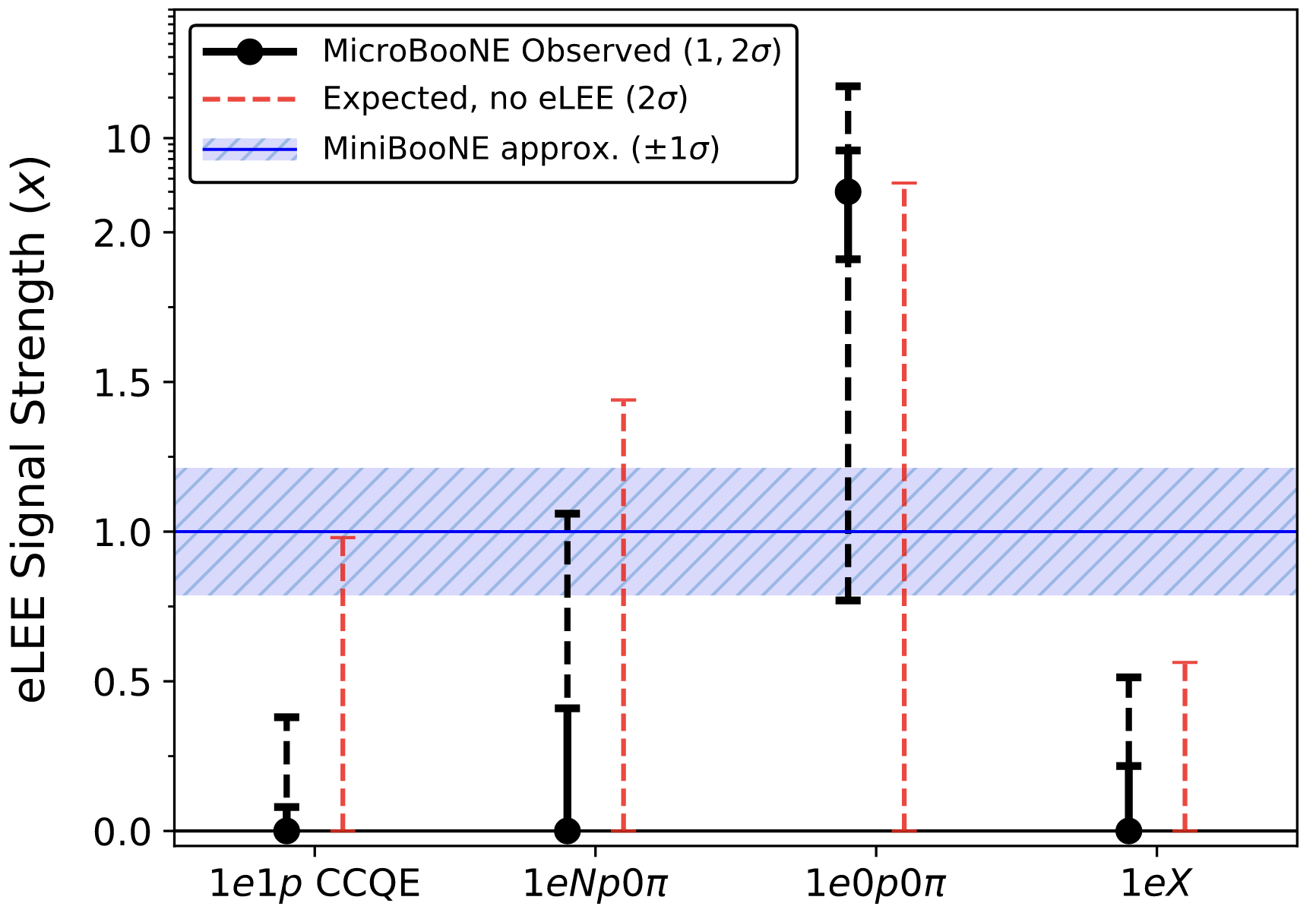
(b)

Figure 5.15: Figure 5.15(a) shows the observation compared to the nominal ($H_{0}$) prediction in all four signal channels from the three MicroBooNE $\nu_{e}$ analyses, including statistical errors on the data points and systematic errors on the prediction. The eLEE prediction ($H_{1}$) is also indicated by the red line. Figure 5.15(b) shows the observed $1\sigma$ and $2\sigma$ confidence intervals on $x_{\rm LEE}$ from all four signal channels. The $2\sigma$ expected sensitivity of each channel is shown in red.

5.3.1 Publication: MiniBooNE and MicroBooNE Combined Fit to a $3+1$ Sterile Neutrino Scenario

The initial results from the MicroBooNE $\nu_{e}$ analyses did not explicitly test short-baseline $\nu_{\mu}\to\nu_{e}$ oscillations from the $3+1$ model. Shortly after the MicroBooNE results came out, two studies appeared assessing the sensitivity of the MicroBooNE $\nu_{e}$ analyses to the $3+1$ model [188, 213]. Following up on this, the MiniBooNE collaboration released the first combined fit to a $3+1$ model using MicroBooNE and MiniBooNE data [102]. This study was led by myself and Austin Schneider. The full Physical Review Letters publication is included below. We considered the two-body CCQE and inclusive MicroBooNE $\nu_{e}$ analyses, as these placed the most stringent constraints on the eLEE model and provided data releases with the requisite detail to perform a $3+1$ fit [116]. The most important result from this study is Figure 2, which indicates that there are still allowed regions in $3+1$ parameter space at the $3\sigma$ confidence level in the MiniBooNE-MicroBooNE combined fit. This was also the first MiniBooNE analysis to account for all three oscillation probabilities in equation 1.36: $\nu_{e}$ appearance, $\nu_{\mu}$ disappearance, and $\nu_{e}$ disappearance. Previous $3+1$ fits to MiniBooNE data have only considered $\nu_{e}$ appearance, as this is the dominant effect in the electron-like channel. However, $\nu_{e}$ and $\nu_{\mu}$ disappearance can have a non-negligible impact on the intrinsic $\nu_{e}$ and misidentified $\nu_{\mu}$ background rate in the MiniBooNE electron-like prediction. The $\nu_{e}$ disappearance probability is also important when considering MicroBooNE data, as the prediction in each MicroBooNE $\nu_{e}$ analysis is dominated by intrinsic $\nu_{e}$ interactions [148, 170]. MicroBooNE has since released official constraints on the $3+1$ model using data from the inclusive $\nu_{e}$ analysis [214]–these constraints are consistent with our implementation.

See pages - of templates/Publications/PhysRevLett.129.201801.pdf See pages - of templates/Publications/MBuB_supplemental.pdf

5.3.2 Publication: Implications of MicroBooNE’s low sensitivity to electron antineutrino interactions in the search for the MiniBooNE excess

The first MicroBooNE results indeed set strong limits on $\nu_{e}$ CC interactions as an explanation for the entire MiniBooNE LEE. However, as pointed out in Ref. [201], this conclusion changes if the MiniBooNE LEE comes instead from $\overline{\nu}_{e}$ CC interactions. This is driven mainly by differences in the low-energy suppression of $\overline{\nu}_{e}$-nucleus and $\nu_{e}$-nucleus cross sections, coming from interference between the vector and axial form factors as well as nucleon binding energy effects. Binding energy effects are especially important in MicroBooNE–within a non-isoscalar nucleus like ⁴⁰Ar, it takes more energy for a $\overline{\nu}_{e}$ to turn a proton into a neutron than it does for a $\nu_{e}$ to turn a neutron into a proton. This is not necessarily the case in MiniBooNE, as ¹²C is an isoscalar nucleus. This study was led by myself and Matheus Hostert. The full Physical Review D publication can be found below. The most important results are shown in Figure 5 and Figure 6, which indicate that the MicroBooNE sensitivity to the MiniBooNE LEE decreases as more of the excess is attributed to $\overline{\nu}_{e}$ rather than $\nu_{e}$ CC interactions. Specifically, the MicroBooNE data are consistent at the $2\sigma$ confidence level with a scenario in which the entire MiniBooNE LEE comes from $\overline{\nu}_{e}$ interactions.

See pages - of templates/Publications/PhysRevD.107.092002.pdf

Chapter 6 Neutrissimos: Heavy Neutral Leptons with a Dipole Moment

In this chapter, we discuss a phenomenological explanation of the MiniBooNE excess involving both an eV-scale sterile neutrino and an MeV-scale heavy neutral lepton (HNL) with an effective transition magnetic moment coupling to active neutrinos. This “mixed model” was introduced in Ref. [27] and refined in Ref. [31]. The HNL in this model is hereafter referred to as a “neutrissimo” [31], a term which has previously been used to describe interacting HNLs in the literature [215, 216].

We begin with a brief overview of the theoretical framework behind neutrissimos. We then motivate the mixed model and discuss its implications for global neutrino experiments. A robust evaluation of the neutrissimo signal in MiniBooNE is performed. For a neutrissimo mass $m_{\mathcal{N}}\sim 500~{}{\rm MeV}$, single photons from visible neutrissimo decay are shown to provide a reasonable explanation of the energy and angular distributions of the MiniBooNE excess. World-leading constraints on neutrissimos are derived using elastic scattering data from the MINER$\nu$A experiment [217, 218, 219]. While the MINER$\nu$A data exclude a large region of parameter space for $m_{\mathcal{N}}=\mathcal{O}(100~{}{\rm MeV})$, they do not rule out the MiniBooNE solution at the 95% confidence level. The details behind this analysis are given in Ref. [31]; the full published manuscript is included in section 6.4.

Publications covered in this chapter for which I held a leading role: [27, 31]

6.1 Dipole-Portal Neutrissimos

The neutrissimo $\mathcal{N}$ is a right-handed neutrino that couples to the active neutrinos through a transition magnetic moment. This coupling is described by the dimension-five dipole operator

$$\mathcal{L}_{D}=d_{\alpha\mathcal{N}}\,\overline{\nu_{\alpha}}\sigma_{\mu\nu}F^{\mu\nu}\mathcal{N}_{R}+\text{ h.c.},$$ (6.1)

where $d_{\alpha\mathcal{N}}$ is the dipole coupling between the right-handed neutrissimo $\mathcal{N}_{R}$ and the left-handed weak flavor eigenstate $\nu_{\alpha}$, and $F^{\mu\nu}=\partial^{\mu}A^{\nu}-\partial^{\nu}A^{\mu}$ is the EM field strength tensor. The dipole coupling has units of inverse energy, as equation 6.1 is an effective operator. This means it is agnostic to the ultraviolet (UV) completion: the short-distance physics generating the dipole coupling at a higher energy scale. Possible UV completions for the dipole operator include (but are not limited to) $SU(2)_{L}\times SU(2)_{R}$ theories [220], leptoquark models [81], and models introducing additional Higgs multiplets or other charged scalars [221, 222, 223, 224]. We will treat neutrissimos within the effective field theory framework throughout this chapter. Figure 6.1 shows a Feynman diagram of the effective operator in equation 6.1. It facilitates a number of new interactions involving the neutrissimo, the most relevant of which are shown in figure 6.2.

Equation 6.1 is only valid below the electroweak scale, as it does not respect $SU(2)_{L}\times U(1)_{Y}$ gauge invariance. Before electroweak symmetry breaking (EWSB), the dipole coupling is described by the gauge invariant dimension six operator

$$\mathcal{L}\supset\frac{1}{\Lambda^{2}}\overline{L_{\alpha}}\widetilde{H}\sigma^{\mu\nu}\mathcal{N}_{R}\left(C_{B}^{\alpha}\,B_{\mu\nu}+C_{W}^{\alpha}\,W^{a}_{\mu\nu}\sigma_{a}\right)+\text{ h.c.},$$ (6.2)

where $\Lambda$ is the UV completion scale, $L_{\alpha}$ is the left-handed lepton $SU(2)_{L}$ doublet, $\widetilde{H}=i\sigma_{2}H^{*}$ is the conjugate Higgs field, and $C_{B}^{\alpha}$ and $C_{W}^{\alpha}$ are the Wilson coefficients for couplings to the $B_{\mu}$ and $W_{\mu}$ vector gauge bosons, respectively. The dipole coupling in equation 6.1 after EWSB is then given by

$$d_{\alpha\mathcal{N}}=\frac{v_{h}}{\sqrt{2}\Lambda^{2}}(C_{B}^{\alpha}\cos\theta_{W}+C_{W}^{\alpha}\sin\theta_{W}),$$ (6.3)

where $v_{h}$ is the Higgs vacuum expectation value and $\theta_{W}$ is the Weinberg angle. Note that couplings are also generated with the $W$ and $Z$ bosons after EWSB, but interactions involving these couplings are suppressed by $G_{F}$ and are thus not as important as the photon coupling.

Transition magnetic moments between different neutrino species have been discussed extensively in the literature [225, 226, 227, 228, 229, 81, 130, 223, 230]. The imprint of heavy neutral leptons with transition magnetic moments in experimental data has received particular attention [130, 81, 231, 123, 124, 126, 127, 232, 233, 234, 235, 236, 135, 237, 238, 239, 240]. One potential complication of this model is that large transition magnetic moments often lead to large Dirac masses $m_{\nu\mathcal{N}}$ for neutrinos [81, 130, 31]. This is because the photon line can typically be removed from figure 6.1, resulting in a contribution to the Dirac mass term $\mathcal{L}\supset m_{\nu\mathcal{N}}\overline{\nu}_{L}\mathcal{N}_{R}$. Dipole coupling strengths of interest to MiniBooNE ($d\sim 10^{-6}$ GeV) would generate Dirac mass contributions $m_{\nu\mathcal{N}}=\mathcal{O({\rm MeV}})$ [81]. Considering a neutrissimo mass $m_{\mathcal{N}}\sim 500$ MeV, the typical seesaw relation of equation 1.23 would predict active neutrino masses $m_{\nu}>>1~{}{\rm eV}$, in conflict with existing limits. This can be remedied by the inverse seesaw mechanism [241, 242], in which the smallness of active neutrino masses comes from approximate lepton number conservation without relying on large right-handed neutrino masses. [81, 31].

Another complication is the potential existence of mass mixing between the neutrissimo and the active neutrinos. This mixing is heuristically given by $U_{\alpha\mathcal{N}}\sim m_{\nu\mathcal{N}}/m_{\mathcal{N}}$ and is large even in the inverse seesaw mechanism [81]. If this operator is not suppressed, the interactions of the neutrissimo are dominated by those involving the $W$ and $Z$ bosons. Any potential mass mixing would be subject to constraints from accelerator neutrino experiments, which can be strong for $m_{\mathcal{N}}=\mathcal{O}(100~{}{\rm MeV})$ [243]. Specifically, searches for HNLs produced in kaon decay at T2K (using the ND280 near detector) [244], E949 [245], and PS191 [246] set upper bounds on the muon-flavor mixing of $|U_{\mu\mathcal{N}}|^{2}\leq 10^{-8}-10^{-9}$ up to the kaon mass threshold of $m_{\mathcal{N}}\sim 400~{}{\rm MeV}$. Within the range $400\leq m_{\mathcal{N}}~{}[{\rm MeV}]\leq 2000$, NuTeV is able to set upper bounds of $|U_{\mu\mathcal{N}}|^{2}\leq 10^{-6}-10^{-7}$ by searching for HNLs produced in $D$ meson decays.

In order to suppress mass mixing, the Dirac mass itself must be small compared to the neutrissimo mass. One possible method to accomplish this is the approximate horizontal $SU(2)_{H}$ symmetry proposed by Voloshin [247]. The idea of an approximate $SU(2)_{H}$ symmetry initially gained popularity as a means to enable the $\nu_{e}$ diagonal/transition magnetic moment solution to the solar neutrino problem [248, 249, 250]. For the heavy neutral lepton case, we consider a scenario in which $(\nu_{L}^{C},\mathcal{N}_{R})$ transforms as a doublet under $SU(2)_{H}$ [251, 81, 224]. The antisymmetric nature of the dipole operator $\overline{\nu}_{\alpha}\sigma_{\mu\nu}F^{\mu\nu}\mathcal{N}_{R}$ in flavor space means that it transforms like a singlet under $SU(2)_{H}$, while the symmetric nature of the Dirac mass term makes it a triplet under $SU(2)_{H}$. Thus, approximate $SU(2)_{H}$ conservation will suppress the Dirac mass contribution from the photon-less version of figure 6.1 while allowing for large contributions to the transition magnetic moment. Though it is not clear the level of fine-tuning required within this model to accommodate the MiniBooNE solution [224], we consider this sufficient motivation to consider a scenario in which the mass mixing operator of the heavy neutrino is negligible compared to the dipole operator. It is also worth pointing out the leptoquark UV completion of the dipole operator proposed in Ref. [81], which can naturally suppress the mass mixing of neutrissimos via an $SU(2)_{H}$ symmetry without the need for significant fine-tuning.

Figure 6.1: Feynman diagram depicting the effective dipole operator of equation 6.1.

(a)

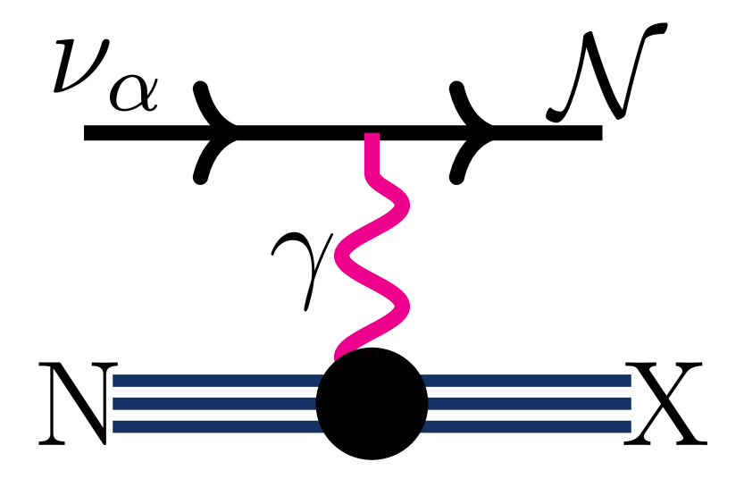
(b)

(c)

Figure 6.2: New interactions involving the neutrissimo that are enabled by the dipole operator in equation 6.1, including three-body $\pi^{0}$ decay (figure 6.2(a)), Primakoff-like upscattering (figure 6.2(b)), and neutrissimo decay (figure 6.2(c)).

6.2 Overview of the Mixed Model

The mixed model consists of the eV-scale sterile neutrino described in section 1.4 and the MeV-scale neutrissimo described above in section 6.1. This model is motivated by the significant tension observed between appearance and disappearance experiments in $3+1$ global fits [93, 12, 11, 252], which comes from strong signals indicating $\nu_{e}$ appearance and $\nu_{e}$ disappearance coupled with the lack of such a signal in the $\nu_{\mu}$ disappearance channel. This tension is measured using the parameter goodness-of-fit (PG) test [253], which uses the test statistic

$$\begin{split}&\chi^{2}_{PG}=\chi^{2}_{\rm global}-(\chi^{2}_{\rm app}+\chi^{2}_{\rm dis}),\\ &N_{PG}=(N_{\rm app}+N_{\rm dis})-N_{\rm global},\end{split}$$ (6.4)

where $\chi^{2}_{\rm global}$, $\chi^{2}_{\rm app}$, and $\chi^{2}_{\rm dis}$ are the total $\chi^{2}$ at the $3+1$ best-fit parameters for global, appearance-only, and disappearance-only experiments, respectively. The number of degrees-of-freedom $N$ is defined similarly. The probability that the appearance and disappearance experiments come from the same underlying $3+1$ model can be calculated using the $\chi^{2}_{PG}$ distribution for $N_{PG}$ degrees-of-freedom.

This tension appears to be driven significantly by MiniBooNE data [27, 12]. Within the Harvard-Columbia-MIT global fit that existed at the time of Ref. [27], the PG test tension decreased from $4.8\sigma$ to $2.5\sigma$ upon removing the MiniBooNE dataset. The allowed regions in $\Delta m_{41}^{2}$-$\sin^{2}2\theta_{\mu e}$ parameter space for the global, appearance-only, and disappearance-only experiments both before and after removing MiniBooNE are shown in figure 6.3 and figure 6.4, respectively. One can see visually that there is more overlap in the $\Delta m^{2}$ dimension between the three different allowed regions after removing MiniBooNE. This is likely because the MiniBooNE excess peaks strongly at low energies, an effect which is difficult to produce in the $3+1$ model, as discussed in section 2.2. The latest MiniBooNE $3+1$ fits discussed in section 5.3.1 specifically show that the oscillation hypothesis under-predicts the excess in the lowest bins of the MiniBooNE electron-like dataset. This behavior drives the global fit to the $\Delta m_{41}^{2}<1~{}{\rm eV}^{2}$ region, in contrast to the higher values ($\Delta m_{41}^{2}\gtrsim 1~{}{\rm eV}^{2}$) preferred by the reactor and gallium anomalies.

The global fit without MiniBooNE, shown in the leftmost panel of figure 6.4, strongly prefers a solution at $\Delta m_{41}^{2}\sim 1~{}{\rm eV}^{2}$ and $10^{-4}\lesssim\sin^{2}2\theta_{\mu e}\lesssim 10^{-3}$. The best fit point is specifically at $\Delta m_{41}^{2}=1.3~{}{\rm eV}^{2}$ and $\sin^{2}2\theta_{\mu e}=6.9\times 10^{-4}$. We take these as our benchmark $3+1$ parameters, which fix the $\nu_{\mu}\to\nu_{e}$ oscillation contribution to the MiniBooNE electron-like channel. The oscillation prediction alone is not sufficient to explain the MiniBooNE LEE; it can only accommodate $\sim 10\%$ of the total excess events and peaks at $E_{\nu}\sim 600~{}{\rm MeV}$, inconsistent with the low-energy nature of the MiniBooNE excess. However, the benefit of these specific oscillation parameters is that they can explain LSND, reactor, and gallium data while remaining consistent with null results from $\nu_{\mu}$ disappearance searches. The impact of different mixing angles within the allowed region of the global fit without MiniBooNE is discussed in Ref. [27], and the impact of the (larger) oscillation contribution predicted by the MiniBooNE-MicroBooNE combined best fit [102] is discussed in Ref. [31].

The remaining majority of the MiniBooNE excess must then come from another source. In the mixed model, we ascribe the bulk of the LEE to the visible decays of neutrissimos. This model works well for MiniBooNE, as neutrissimos can be produced abundantly in the BNB through the first two diagrams in figure 6.2: Primakoff upscattering $\nu A\to\mathcal{N}A$ and the three-body decay $\pi^{0}\to\gamma\nu\mathcal{N}$. The third diagram, neutrissimo decay $\mathcal{N}\to\nu\gamma$, could then provide a source of extra photons in MiniBooNE. As discussed in chapter 2, these photons would show up in the electron-like sample due to MiniBooNE’s reliance on Cherenkov rings for particle identification. Models of heavy neutrino decay to single photons have been previously considered as a solution to the MiniBooNE anomaly [123, 254, 124, 125, 126, 127, 128, 129, 130, 131, 132, 133, 134, 135]. We extend upon these studies by performing a robust analysis of the neutrissimo model in MiniBooNE within the context of the mixed model. This analysis is described in detail in the next section. It turns out that compared to the $3+1$ model, neutrissimo decays are more consistent with the energy and angular distributions of the MiniBooNE excess. Thus there are two distinct advantages of the mixed model: (1) it can provide an explanation for other anomalies in the neutrino sector while relieving tension in global $3+1$ fits, and (2) it can provide a better explanation of the MiniBooNE excess itself.

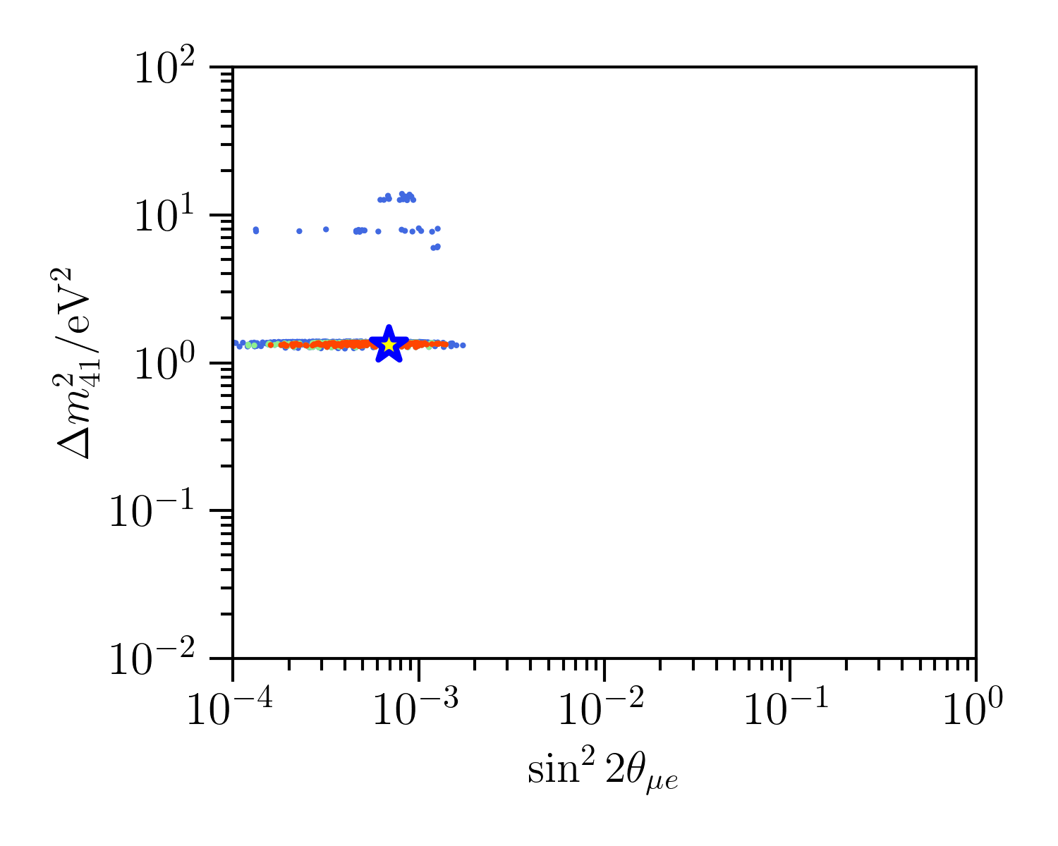
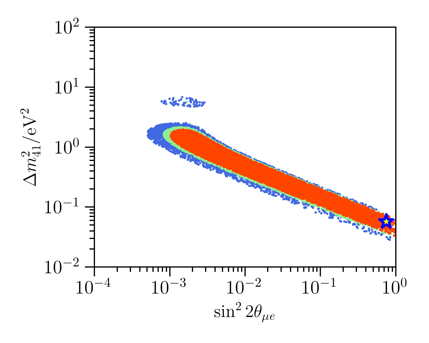
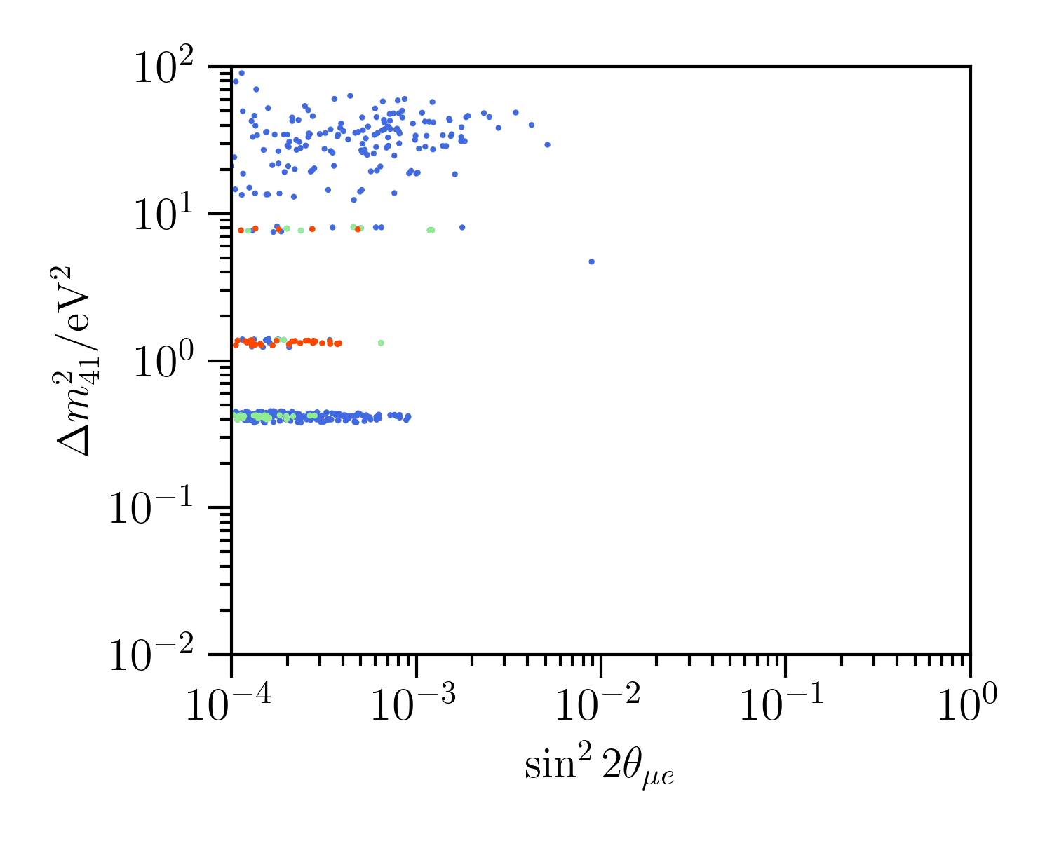
Figure 6.3: $3+1$ global fits including MiniBooNE, considering global (left), appearance-only (middle), and disappearance-only (right) experiments. The allowed regions in $3+1$ parameter space at the 90%, 95%, and 99% confidence levels are shown by the red, green, and blue points, respectively. The best-fit point is indicated by the star.

Figure 6.4: $3+1$ global fits without MiniBooNE, considering global (left), appearance-only (middle), and disappearance-only (right) experiments. The allowed regions in $3+1$ parameter space at the 90%, 95%, and 99% confidence levels are shown by the red, green, and blue points, respectively. The best-fit point is indicated by the star.

6.3 Neutrissimos in MiniBooNE

The analysis presented in Ref. [27] used a custom simulation to estimate the single photon event rate from neutrissimo decays in the MiniBooNE detector. The updated MiniBooNE analysis in Ref. [31] relied instead on the public LeptonInjector  software package, which will be described in more detail in section 6.3.1. In Ref. [27] we considered neutrissimo production via both $\pi^{0}\to\gamma\nu\mathcal{N}$ decays and $\nu A\to\mathcal{N}A$ Primakoff upscattering. The former process was estimated using the Sanford-Wang parameterization of the $\pi^{0}$ production rate at the BNB ] [110, 14] and was found to be negligible for the dipole parameters of interest to MiniBooNE. We therefore explicitly ignored this process, considering Primakoff upscattering as the sole neutrissimo production mechanism.

The $\nu_{\alpha}A\to\mathcal{N}A$ upscattering rate was calculated using the differential cross section with respect to the Mandelstam variable $t=Q^{2}=(p_{\mathcal{N}}-p_{\nu})^{2}$ [27, 130, 255, 232],

$$\begin{split}\frac{d\sigma_{\nu_{\alpha}A\to\mathcal{N}A}}{dt}=\frac{2\alpha d_{\alpha}^{2}}{M}\bigg{[}&F_{1}^{2}(t)\Big{(}\frac{1}{E_{r}}-\frac{1}{E_{\nu}}+m_{\mathcal{N}}^{2}\frac{E_{r}-2E_{\nu}-M}{4E_{\nu}^{2}E_{r}M}+m_{\mathcal{N}}^{4}\frac{E_{r}-M}{8E_{\nu}^{2}E_{r}^{2}M^{2}}\Big{)}\\ +&\frac{F_{2}^{2}(t)}{4M^{2}}\Big{(}\frac{2M}{E_{\nu}^{2}}((2E_{\nu}-E_{r})^{2}-2E_{r}M)+m_{\mathcal{N}}^{2}\frac{E_{r}-4E_{\nu}}{E_{\nu}^{2}}+\frac{m_{\mathcal{N}}^{4}}{E_{\nu}^{2}E_{r}}\Big{)}\bigg{]},\end{split}$$ (6.5)

where $\alpha$ is the fine structure constant, $d$ is the dipole coupling, $E_{\nu}$ is the SM neutrino energy, $m_{\mathcal{N}}$ is the mass of the heavy neutrino, $M$ is the target mass, $t=-(p_{\mathcal{N}}-p_{\nu})^{2}$ is the momentum transfer, $E_{r}=-t/2M$ is the target recoil energy, and $F_{1/2}(t)$ are the electric/magnetic target form factors, respectively. Note that the term proportional to $E_{r}m_{N}^{4}$ in the $F_{1}$ line only exists for spinless nuclei, and must be replaced for nonzero spin nuclei [127]. In the case of coherent scattering off of a nucleus, $F_{1}$ receives a $Z^{2}$ enhancement and is therefore dominant over $F_{2}$. Thus, we explicitly neglect the $F_{2}$ term for this analysis. In Ref. [27], $F_{1}$ was calculated using a dipole parameterization. However, since the dipole approximation tends to underestimate the cross section at high squared momentum transfer $Q^{2}$, Ref. [31] updated to the Fourier-Bessel parameterization,

$$F^{\rm FB}(Q)=Z^{2}N\frac{\sin(QR)}{QR}\sum_{n}\frac{(-1)^{n}a_{n}}{n^{2}\pi^{2}-Q^{2}},$$ (6.6)

where $Z$ is the proton number of the struck nucleus, $N$ is a normalization factor ensuring $F^{\rm FB}(0)=1$, and $a_{n}$ are coefficients obtained from nuclear scattering data [256, 257, 258, 259]. For the case of inelastic upscattering off of individual nuclei, we use the nucleon electric and magnetic form factors discussed in the appendix of Ref. [27]. Inelastic upscattering exhibits only a linear enhancement in the number of protons and neutrons, which suppresses its effect compared to the $Z^{2}$ enhancement of the coherent upscattering cross section. Ref. [31] also includes contributions from the sub-dominant helicity-conserving channel of both the elastic and inelastic upscattering cross sections.

The total upscattering cross section was obtained by integrating equation 6.5 over the physical momentum transfer range [130]. The overall neutrissimo production rate via upscattering in the BNB was then calculated using this cross section in combination with the density of each nuclear and nucleon target available along the BNB. These include nuclei in the bedrock and air between the BNB target and the detector, as well as carbon and hydrogen nuclei in the detector itself. The bedrock composition is defined in table 6.1 and is considered to have a density of 2.9 g/cm³. Upscattering in the bedrock (detector) is more important for long-lived (short-lived) neutrissimos. The kinematics of the outgoing neutrissimo were fixed by sampling a momentum transfer $t$ according to equation 6.5, which consequently determines the nuclear recoil energy $E_{r}=-t/2M$ as well as the neutrissimo energy and scattering angle [127],

$$\begin{split}&E_{\mathcal{N}}=E_{\nu}-E_{r},\\ &\cos(\theta)=\frac{E_{\nu}-E_{r}-ME_{r}/E_{\nu}-m_{\mathcal{N}}^{2}/2E_{\nu}}{\sqrt{E_{\nu}^{2}+E_{r}^{2}-2E_{\nu}E_{r}-m_{\mathcal{N}}^{2}}}.\end{split}$$ (6.7)

One can rewrite equation 6.5 to isolate an overall $1/t^{2}$ prefactor, indicating a preference for $t\approx 0$ and thus $\cos\theta\approx 1$ for this process.

After neutrissimos are produced, they will decay via the process $\mathcal{N}\to\nu\gamma$. The decay width $\Gamma$ and lab-frame decay length $L_{\rm decay}$ of this process are given by  [130, 27, 31]

$$\begin{split}&\Gamma=\frac{d^{2}m_{\mathcal{N}}^{3}}{4\pi},\\ &L_{\rm decay}=4\pi\frac{\beta E_{\mathcal{N}}}{d^{2}m_{\mathcal{N}}^{4}},\end{split}$$ (6.8)

where

$$d\equiv\Big{(}\sum_{\alpha}|d_{\alpha N}|^{2}\Big{)}.$$ (6.9)

Considering the dipole parameters preferred by the MiniBooNE excess, the typical neutrissimo decay length at BNB energies is $L\lesssim 1~{}{\rm m}$. The probability of decaying within the MiniBooNE detector is then

$$P_{\rm decay}=\exp\bigg{(}\frac{-L_{\rm enter}}{L_{\rm decay}}\bigg{)}-\exp\bigg{(}\frac{-L_{\rm exit}}{L_{\rm decay}}\bigg{)},$$ (6.10)

where $L_{\rm enter}$ and $L_{\rm exit}$ are the distance along the neutrissimo path from the upscattering location to the entrance and exit of the MiniBooNE detector, respectively. Assume the neutrissimos are Dirac particles, their differential decay which is given by [131, 135]

$$\frac{d\Gamma}{d\cos\theta}=\frac{1}{2}(1+\alpha\cos\theta),$$ (6.11)

where $\alpha=1$ ($\alpha$ = -1) for the decay of a right-handed (left-handed) heavy neutrino, and vice versa for the antineutrino case.

In Ref. [27] and Ref. [31], we used the combination of the production rate from equation 6.5 and the decay rate from equation 6.8 to compute the single photon rate from neutrissimo decay in MiniBooNE.

Nucleus	Z	A	Crust Mass Fraction	Crust Atomic Fraction	Nuclear Radius [MeV-1]
O	8	16	0.466	0.627	0.00218
Si	14	28	0.277	0.213	0.00252
Al	13	27	0.081	0.065	0.00247
Fe	26	56	0.05	0.019	0.00301
Ca	20	40	0.037	0.02	0.00281
K	19	39	0.027	0.015	0.00277
Na	11	23	0.026	0.024	0.00241
Mg	12	24	0.015	0.013	0.00247
Ti	22	48	0.004	0.002	0.0029
P	15	31	0.001	0.001	0.00257

Table 6.1: Relevant parameters of the ten most abundant nuclei in the Earth’s upper crust according to [32]

6.3.1 Simulation in LeptonInjector

As stated above, Ref. [27] built a custom simulation to assess the neutrissimo model in MiniBooNE. Ref. [31] instead performed the MiniBooNE simulation using the LeptonInjector software package. LeptonInjector was originally developed within the IceCube collaboration [260] to simulate the interactions of high-energy neutrinos within their detector; however, this version was not suitable to handle the neutrissimo model out-of-the-box. A series of updates were made to LeptonInjector, led by Austin Schneider and myself, in order to carry out the study described here. These include (but are not limited to):

• Support for the input of total and differential cross section tables.

• Support for a wide variety of detector subsystem geometries, including extruded polygons.

• Ability to simulate a tree of secondary interactions following the initial interaction.

• Ability to calculate event weights for general interaction trees.

• Support for a combination of cross sections and decays as possible interactions for a given particle.

• Support for a fiducialization requirement to improve the computational efficiency.

The current version of LeptonInjector is suitable for general purpose studies of particle interactions in a wide variety of detectors. It was presented at the March 2023 Coherent-CAPTAIN-Mills Workshop [261] and is publicly available on GitHub [262]. While LeptonInjector is written in C++, the classes and methods are importable as a library in Python [263].

We now briefly review the LeptonInjector-based MiniBooNE analysis presented in Ref. [31]. Neutrinos are first injected along the beam axis with energies sampled from the BNB flux [14]. The upscattering location is then sampled according to the material-dependent interaction length along the neutrino path. The interaction length in each material is calculated via upscattering cross section tables computed using DarkNews [264]. In order to optimize the efficiency of the simulation, neutrinos are required to undergo a Priamkoff upscattering interaction within three neutrissimo decay lengths of the MiniBooNE detector. The kinematics of the neutrissimo are fixed by sampling the differential cross section in equation 6.5, calculated in tabular format using DarkNews. The decay location of the neutrissimo is then sampled according to the lab frame decay length in equation 6.8. If the neutrissimo path crosses the detector volume, it is required to decay within or just before the detector, further optimizing the efficiency of the simulation. Once a photon is generated, we sample the pair-production location according to the radiation length of each traversed material, which we use to perform a robust fiducialization cut. The weight of each event is calculated by comparing the generation probability of each sampled quantity (e.g. the energy/direction of the initial neutrino, the kinematics of the produced neutrissimo/photon, and the upscattering/decay locations) to the specified physical probability distribution. The flux units provided in Ref. [14] allow us to compute event weights in units of POT^-1.

Figure 6.5 shows a schematic depiction of the LeptonInjector neutrissimo simulation in MiniBooNE, which incorporates 541 m of bedrock, a 9 m-radius spherical air-filled detector hall, and the 6.1 m-radius spherical mineral oil detector. The result of this procedure is a robust Monte Carlo sample of single photons in MiniBooNE from neutrissimo decay. The kinematic variables of each observable photon have been carefully computed, and the detailed treatment of the geometry of the MiniBooNE detector hall allows for a realistic estimation of the fiducialization requirement. While the latter point is not necessarily vital for the relatively simple MiniBooNE detector, it is much more important when considering the complex MINER$\nu$A detector for the analysis discussed in section 6.4. The careful treatment of new physics models enabled by LeptonInjector is essential for differentiating between the many proposed explanations of MiniBooNE, both when determining the preferred region in model parameter space from MiniBooNE data and when determining constraints from other experiments. This is one of the intended use cases motivating our recent public release of LeptonInjector [262].

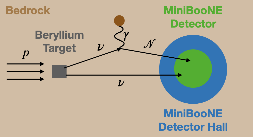
(a)

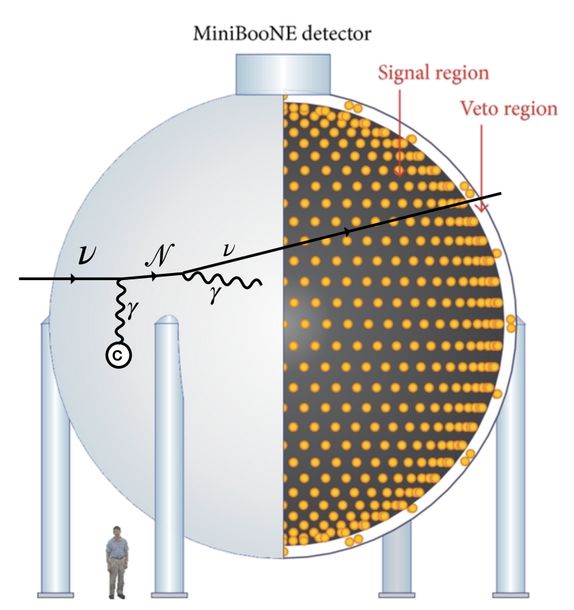
(b)

Figure 6.5: Schematic depiction of the neutrissimo model in MiniBooNE as simulated using LeptonInjector. Figure 6.5(a) shows the simulation of Primkaoff upscattering along the beamline, and figure 6.5(b) shows an example of upscattering, neutrissimo decay and pair-production within the MiniBooNE detector.

6.3.2 Fits to the MiniBooNE Excess

After performing the procedure outlined in section 6.3.1, we down-weighted each event according to a linear parameterization of the MiniBooNE photon detection efficiency [27, 265]. We also imposed a reconstruction threshold on the true photon kinetic energy requiring $E_{\gamma}>140~{}{\rm MeV}$. The energy (angle) of the photon was smeared according to a power-law (quadratic) fit to a MiniBooNE single electromagnetic shower simulation sample [266]. The typical resolution in the energy (angular) distribution was 10% ($3^{\circ}$) for the photons generated in this model, consistent with values reported by MiniBooNE [267].

After these steps, the simulated events could then be used to estimate the single photon rate from neutrissimo decays in the $E_{\nu}^{\rm QE}$ and $\cos\theta$ distributions of MiniBooNE’s electron-like sample. We performed a separate fit to the MiniBooNE excess in each distribution. After subtracting the SM prediction and the oscillation prediction from the global fit without MiniBooNE, we calculated a $\chi^{2}$ test statistic between the data and the neutrissimo prediction throughout a grid of points in $d_{\mu\mathcal{N}}$-$m_{\mathcal{N}}$ parameter space. For the $E_{\nu}^{\rm QE}$ distribution, we used the MiniBooNE electron-like covariance matrix provided in the data release [268] associated with Ref. [10]. The MiniBooNE collaboration has not released any information regarding systematic uncertainty in the $\cos\theta$ distribution; therefore, we assign an uncorrelated fractional systematic uncertainty of 13% in this distribution, consistent with the overall level in the $E_{\nu}^{\rm QE}$ distribution. We compute confidence regions in neutrissimo parameter space using the $\Delta\chi^{2}$ test statistic, assuming Wilks’ theorem [26] for two degrees of freedom.

Figure 6.6 shows the 95% and $3\sigma$ confidence level allowed regions in neutrissimo parameter space from the MiniBooNE $E_{\nu}^{\rm QE}$ and $\cos\theta$ distributions. These allowed regions come from Ref. [31], which is intended to supersede the results in Ref. [27]. This is because Ref. [31] makes a number of improvements upon the analysis in Ref. [27], including the use of a more robust nuclear electromagnetic form factor and a more detailed simulation within LeptonInjector. One can see from figure 6.6 that the energy and angular distributions of the MiniBooNE excess prefer different regions of parameter space. This is because the angular distribution has a not-insignificant component at large angles, $-1\leq\cos\theta\leq 0$, as shown in figure 2.6(b). Larger neutrissimo masses are required to explain this region, as such neutrissimos will have a lower Lorentz boost and thus result in a photon with broader lab-frame angles with respect to the beamline. This is in contrast with the energy distribution, which prefers lower neutrissimo masses such that the lower energy part of the BNB neutrino flux is not kinematically forbidding from upscattering into a neutrissimo. The difference between preferred regions of the energy and angular distributions in such visible heavy neutrino decay models has been discussed previously in the literature [135, 128]; however, our study is the first comprehensive analysis of the compatibility of both distributions. Our results in figure 6.6 indicate an overlap between the allowed regions of the $E_{\nu}^{\rm QE}$ and $\cos\theta$ allowed regions at the 95% C.L. Figure 6.7 shows comparisons between the MiniBooNE excess in each distribution and the mixed model prediction, considering the neutrissimo model indicated by the black star in figure 6.6, which is near this 95% C.L. overlap. One can see that the oscillation contribution to the MiniBooNE LEE in this model is indeed small compared with the neutrissimo contribution. A larger oscillation contribution might help explain the $-1\leq\cos\theta\leq 0$ region of the excess–this point is discussed further in section 6.4. That being said, the mixed model does a better job of predicting the excess in the lowest-energy region. This can be seen by comparing the compatibility between data and prediction in the first two bins of figure 6.7(a) to that in figure 2.5(a).

There are a number of existing constraints on the neutrissimo model in the $10\leq m_{\mathcal{N}}~{}[{\rm MeV}]\leq 1000$ regime, as indicated by the grey regions in figure 6.6. These include Super-Kamiokande [237, 233], Borexino [233], Supernova 1987A [130, 81], LSND [130], CHARM-II [232], and NOMAD [231]. See section 6.4 for a more detailed discussion on each constraint. We briefly note that the overlap in the 95% allowed regions in MiniBooNE falls close to the NOMAD constraint derived in Ref. [231], which may motivate a re-analysis of the NOMAD data.

Finally, we remind the reader that any explanation of MiniBooNE must be compatible not only with the energy and angular distributions of the excess but also with the timing distribution [10]. Specifically, the new physics events cannot experience time delays $\Delta t\gtrsim 10~{}{\rm ns}$. This was studied within the context of the neutrissimo model in Ref. [27]. As shown in figure 6.8, neutrissimos with $m_{\mathcal{N}}\sim 500~{}{\rm MeV}$ have time delays $\Delta t\sim 1~{}{\rm ns}$, certainly within the constraint imposed by the MiniBooNE timing distribution. This is because in the region of parameter space preferred by MiniBooNE, neutrissimos tend to be very short-lived and must therefore be produced via upscattering off of nuclei in the detector. As such, the total travel time is dominated by the original speed-of-light neutrino.

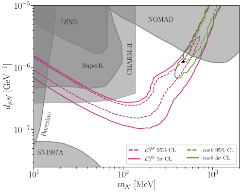
Figure 6.6: Allowed regions at the 95% and $3\sigma$ confidence level in $d_{\mu\mathcal{N}}$-$m_{\mathcal{N}}$ obtained through fits to the MiniBooNE excess in the $E_{\nu}^{\rm QE}$ and $\cos\theta$ distributions. Existing $2\sigma$ constraints on this model are indicated by the grey regions.

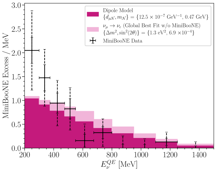
(a)

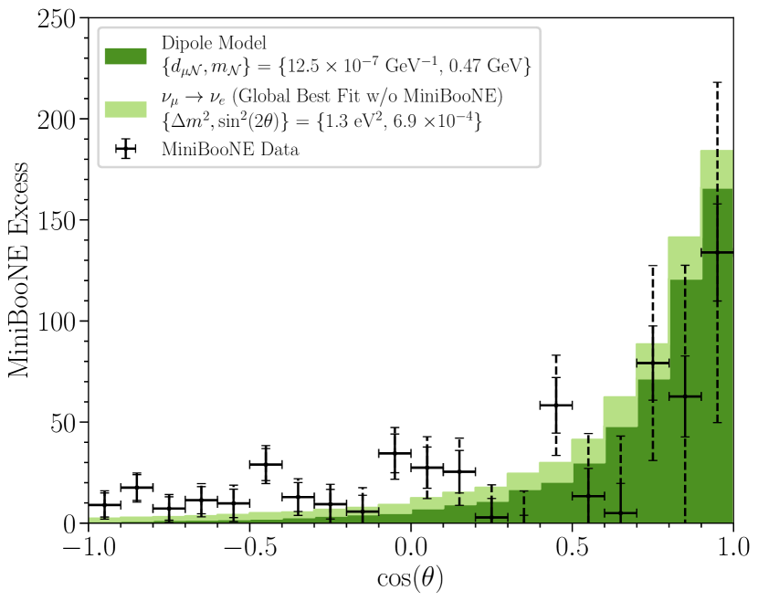
(b)

Figure 6.7: Figure 6.7(a) and figure 6.7(b) show the $E_{\nu}^{\rm QE}$ and $\cos\theta$ distributions of the MiniBooNE excess, respectively, compared with the prediction from the neutrissimo model indicated by the black star in figure 6.6. The oscillation contribution from the $3+1$ global fit without MiniBooNE is also shown.

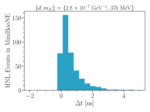
Figure 6.8: The added time delay in MiniBooNE for a neutrissimo with the indicated parameters, as calculated in Ref. [27].

6.4 Publication: Dipole-coupled neutrissimo explanations of the MiniBooNE excess including constraints from MINERvA data

We close this chapter with a presentation of Ref. [31]. The work was led by myself, Matheus Hostert, and Austin Schneider. The full Physical Review D publication is included below. As described in section 6.3, this study performed a more detailed analysis of the mixed model described in section 6.2 as a solution to the MiniBooNE excess. We also derived world-leading constraints on the neutrissimo model using neutrino electron elastic scattering data from the MINER$\nu$A experiment [217, 218, 219]. While these constraints are strong, they do not rule out the overlap in the 95% C.L. allowed regions from the MiniBooNE energy and angular distributions shown in figure 6.6. As shown in Figure 8 of the paper below, this is a result of the strict kinematic cuts employed in the MINER$\nu$A elastic scattering analysis. If these cuts are relaxed, MINER$\nu$A should be sensitive to the MiniBooNE neutrissimo solution in the mixed model. The most important result from this study is given in Figure 10, which shows the surviving parts of the MiniBooNE allowed regions in neutrissimo parameter space after the MINER$\nu$A constraints are incorporated. The dashed lines in the right panel indicate contours of constant number of neutrissimo decays in the MINER$\nu$A fiducial volume before any cuts are applied. One can see that MINER$\nu$A should have $10^{4}-10^{5}$ events before cuts within the MiniBooNE-preferred region of parameter space. We also test the implications of weak-flavor-conserving UV-completions of the dipole operator of equation 6.1, which predict $d_{\alpha\mathcal{N}}\propto m_{\ell_{\alpha}}$ and thus a large $d_{\tau}$. This scenario mostly alters the allowed regions and constraints in the lower mass region of parameter space without impacting the MiniBooNE solution.

Note: while the published version of this article uses the phrase “heavy-neutral-lepton” in the title, the authors prefer the arXiv title given above.

See pages - of templates/Publications/PhysRevD.107.055009.pdf

Chapter 7 The Coherent CAPTAIN-Mills Experiment

We now turn to the Coherent CAPTAIN-Mills (CCM) experiment at Los Alamos National Laboratory (LANL). CCM uses a 10-ton cylindrical liquid argon detector to observe the scintillation and Cherenkov light generated by the interactions of particles produced at the Lujan beam dump facility [30]. CCM was originally designed to detect $\nu_{\mu}$ produced by $\pi^{+}$ decay-at-rest via coherent elastic neutrino-nucleus scattering (CE$\nu$NS) [269]. Given the baseline and neutrino energy accessible to the CCM detector, any deficit in this rate would be smoking-gun evidence for $\nu_{\mu}$ disappearance via a sterile neutrino [30]. In order to realize this physics goal, CCM was built to maximize photon yield and thus minimize the detection energy threshold. This setup makes CCM an ideal detector to search for potential light dark matter (DM) particles produced in the Lujan beam dump, including $U(1)^{\prime}$ vector-portal DM [30], leptophobic vector-portal DM [270], and axion-like particles (ALPs) [271]. CCM120, a 120-PMT prototype detector, completed a six-week engineering run in Fall 2019, which was used to set constraints on these models. The full 200-PMT CCM200 detector is funded for a three-year physics run at the Lujan facility, which began in Summer 2022. Results from this dataset will set strong constraints on the DM models listed above as well as a variety of additional beyond-the-Standard-Model (BSM) scenarios.

In this chapter, we discuss the projects within CCM in which I was involved during my time as a graduate student. These include the fabrication of veto PMT assemblies for CCM200, the investigation of Cherenkov light detection as a powerful background rejection technique in CCM, and the evaluation of CCM’s sensitivity to the neutrissimo model from chapter 6.

7.1 The CCM Beamline and Detector

The CCM detector operates at the Lujan beam dump facility of the Los Alamos Neutron Science Center (LANSCE) [272, 273]. At LANSCE, protons are accelerated to 800 MeV in the proton storage ring and bunched before impinging vertically downward on the Lujan tungsten target at a rate of 20 Hz. The bunches contain $\sim 3.1\times 10^{13}$ protons each and are delivered in a $280~{}{\rm ns}$ triangular pulse. The beam spills occur at a rate of 20 Hz, corresponding to a duty factor of $\sim 5\times 10^{-6}$. This low duty factor is essential for isolating prompt signal events from background, setting the Lujan facility apart from similar beam dump sources. A cascade of particles is produced when protons hit the tungsten target. The target is housed within a cylindrical target-moderator-reflector-shield (TMRS) which provides immediate shielding around the tungsten disks as well as moderators to control neutron output [28], as shown in figure 7.1. The TMRS itself is surrounded by an additional 4 m of steel shielding. Though the primary objective of the Lujan beam dump is neutron production, proton collisions also create pions, electrons, photons, and potential DM particles. Neutrinos are created via the $\pi^{+}\to\nu_{\mu}(\mu^{+}\to\overline{\nu}_{\mu}\nu_{e}e^{+})$ decay chain, as $\pi^{-}$ dominantly capture on nuclei instead of decaying. The total neutrino flux produced by the Lujan source for each neutrino species in this decay chain is $4.74\times 10^{5}~{}\nu/{\rm cm}^{2}/s$ at the CCM120 location (20 m from the tungsten target). The $\pi^{+}$ come to rest in the target before decaying, leading to the neutrino energy distributions shown in figure 7.2(a). Figure 7.2(b) shows the timing profile of different particles produced in the beam dump at the CCM120 location. This timing distribution is essential for separating $\nu_{\mu}$ from $\pi^{+}$ decay-at-rest and speed-of-light DM particles in the prompt region from delayed non-relativistic neutron backgrounds. This is the main strategy behind the CCM physics analyses.

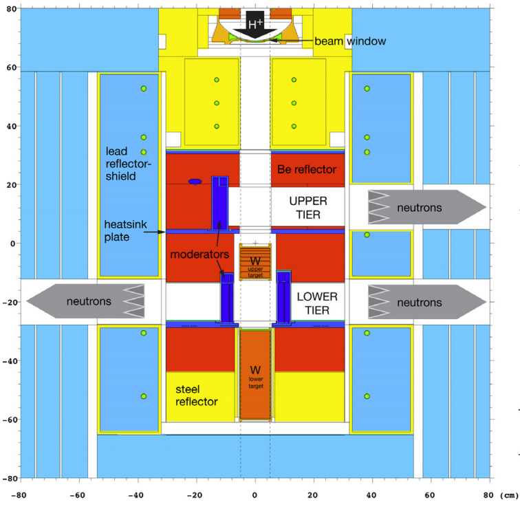
Figure 7.1: Schematic depiction of the Lujan TMRS Figure from Ref. [28].

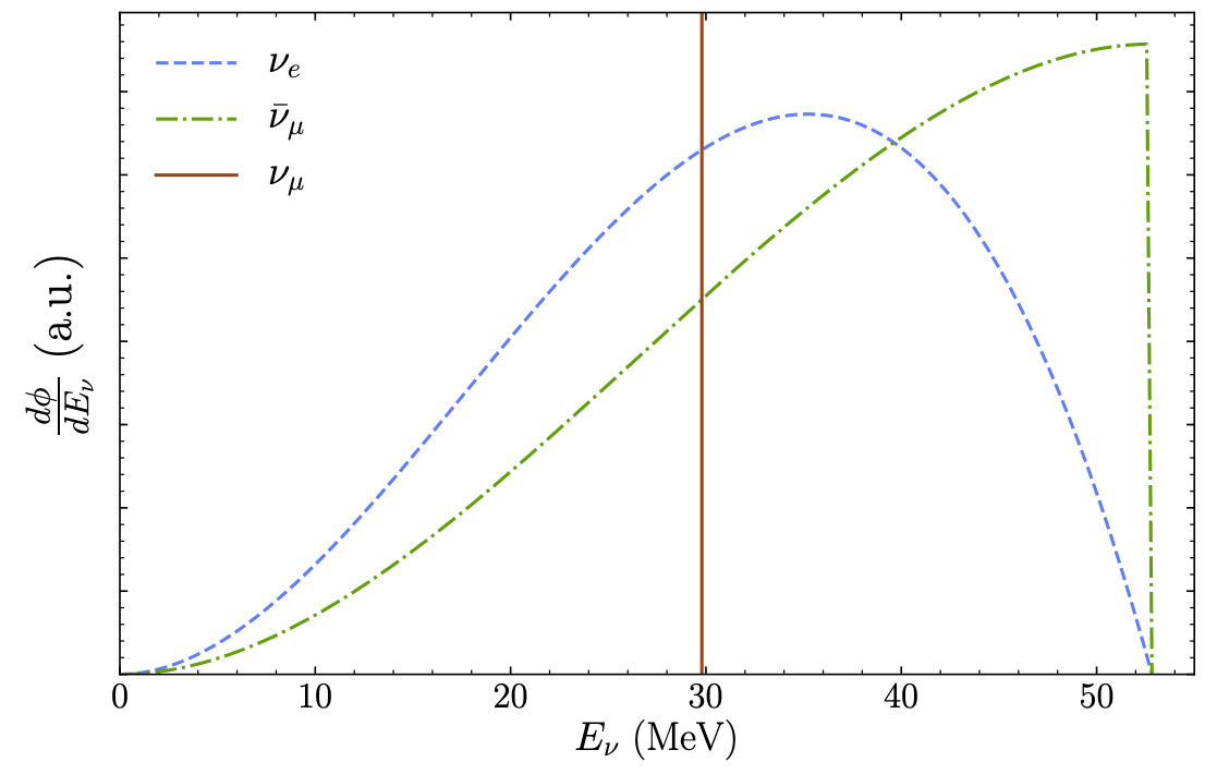
(a)

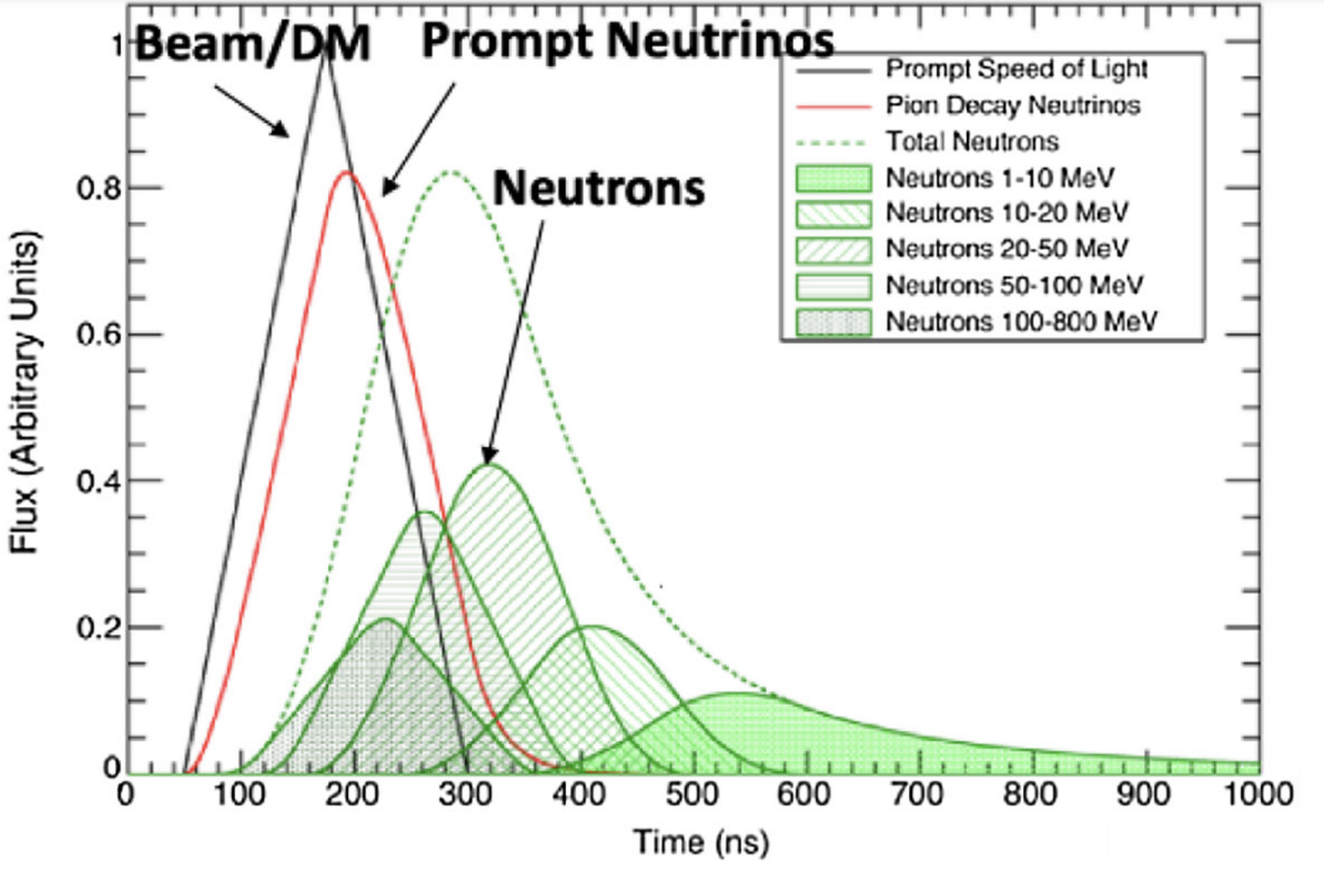
(b)

Figure 7.2: Figure 7.3(a), from Ref. [29], shows the energy distribution of $\pi^{+}$ decay-at-rest neutrinos from the Lujan beam dump source. Figure 7.2(b), from Ref. [30], shows the timing distribution of particles produced in the Lujan beam dump source after traveling through the TMRS.

The CCM detector is a 10-ton cylindrical volume of liquid argon 2.58 m diameter and 2.25 m in height. CCM repurposes the cryostat used by the Cryogenic Apparatus for Precision Tests of Argon Interactions with Neutrinos (CAPTAIN) experiment [274]. In order to take advantage of the timing information discussed above, CCM relies on the fast scintillation light produced when particles interact in the detector, which is emitted on a characteristic time scale of $\mathcal{O}(ns)$. Scintillation light in liquid argon was discussed in section 3.1.3 within the context of the MicroBooNE experiment. In order to collect this scintillation light, the CCM200 detector is instrumented with 200 8-inch Hamamatsu R5912-mod2 PMTs, the same used in the MicroBooNE light collection system described in section 3.1.3. A schematic drawing of this detector is shown in figure 7.3(a). 80 PMTs are arranged uniformly on the top and bottom of the detector, while 120 PMTs are arranged in five rows around the barrel. The CCM120 engineering run only included the PMTs around the barrel. 80% of the PMTs are coated with TPB, which shifts the 128 nm argon wavelength to the visible regime where it can be detected by the PMTs. Additionally, the walls of the detector are covered in reflective foils that are evaporatively coated with TPB. The remaining 20% of PMTs are not coated with TPB and are thus not sensitive to the direct scintillation light produced in the detector. They are only able to observe photons after they are re-emitted by a TPB-coated surface somewhere else in the detector, either on another PMT or on the reflective foils. The presence of uncoated PMTs breaks the degeneracy of the detector response to 128 nm light, helping determine the TPB properties during the calibration process. This point will be important later in section 7.2. Figure 7.3(b) shows an image of the interior PMTs of the CCM200 detector, in which the dull (reflective) hemispheres correspond to coated (uncoated) PMTs. The voltage output from each PMTs is carried through warm cables to a series of CAEN VX1730 boards, which digitize the PMT signals at a rate of 500 MHz. While the beam is running, the digitizers are triggered at a rate of 22.2 Hz, which includes the beam trigger (20 Hz), random strobe trigger (1.1 Hz), and light-emitting-diode (LED) trigger (1.1 Hz). For each trigger, 16 $\mu$s of waveform data on each PMT are saved.

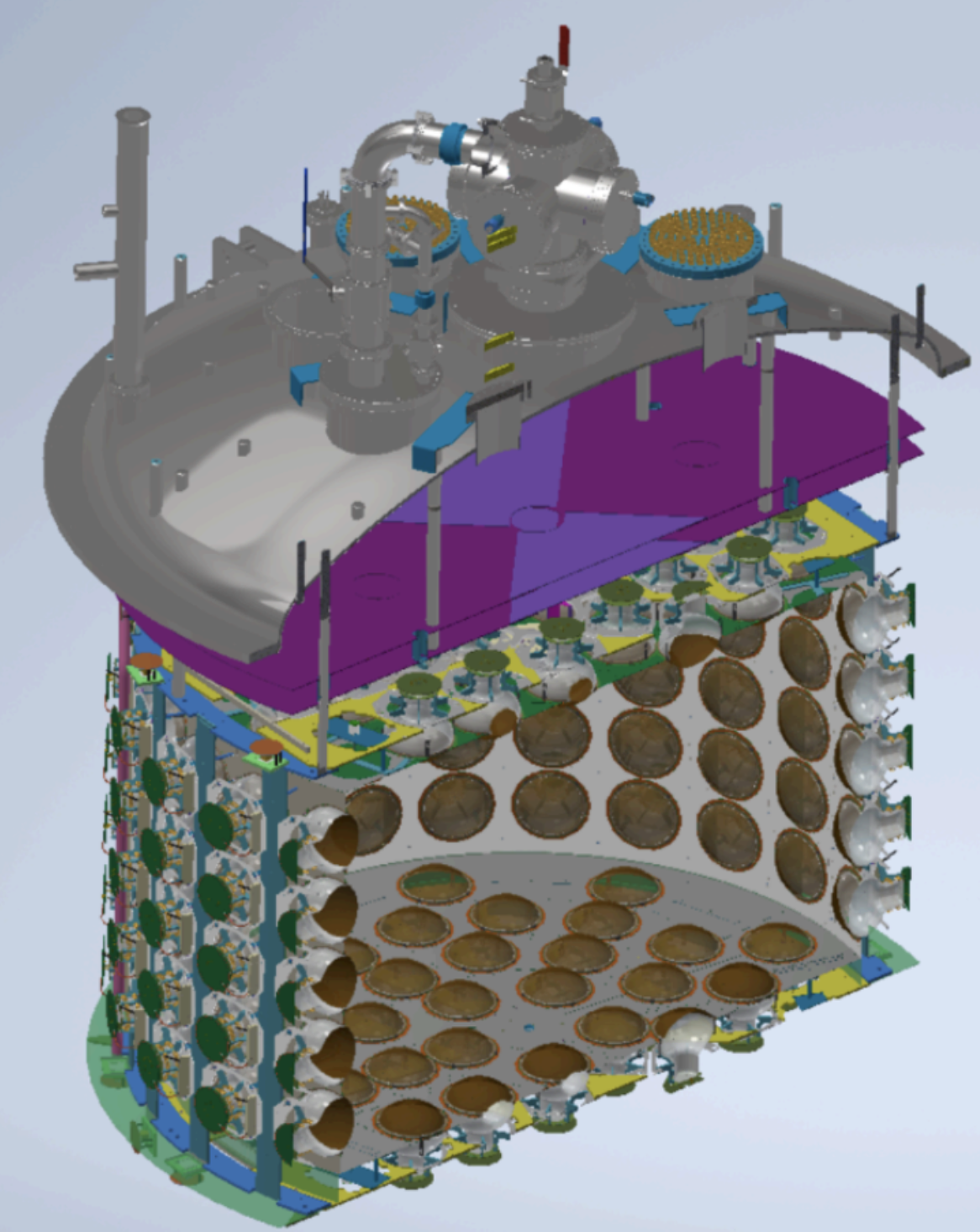
(a)

(b)

Figure 7.3: Figure 7.3(a) shows a schematic 3D rendering of the CCM200 detector. Figure 7.3(b) shows an image of the interior of the CCM200 detector.

CCM200 also houses an additional 40 veto PMTs outside of the fiducial volume to identify and reject events that originate outside of the fiducial volume. These veto PMTs observe light The CCM120 detector used only 28 veto PMTs, of which 5 were the same 8-inch Hamamatsu R5912-mod2 PMTs used in the inner volume and 23 were 1-inch Hamamatsu PMTs. An additional 20 1-inch veto PMTs were assembled and tested at MIT in Summer 2021. Each PMT was assembled into the mounts shown in figure 7.4, which included an acrylic window in front of the photocathode and a custom base circuit for reading out the PMT signal. The acrylic windows were coated with a mixture comprising 1 g of TPB, 1 g of polystyrene, and 50 mL of (very pungent) toluene. The PMTs were tested in a light-tight box with an LED, as shown in figure 7.5. The LED was pulsed via a function generator at 1 V and 2 V, leading to the average veto PMT response shown in figure 7.5. The overshoot observed in these waveforms came largely from the custom breadboard “splitter” circuit assembled for this study, which separated transient PMT signals from high voltage. As the official splitter circuit used by CCM is more robust to ringing, this response was deemed sufficient for CCM200, and the 1-inch veto PMTs were shipped back to LANL.

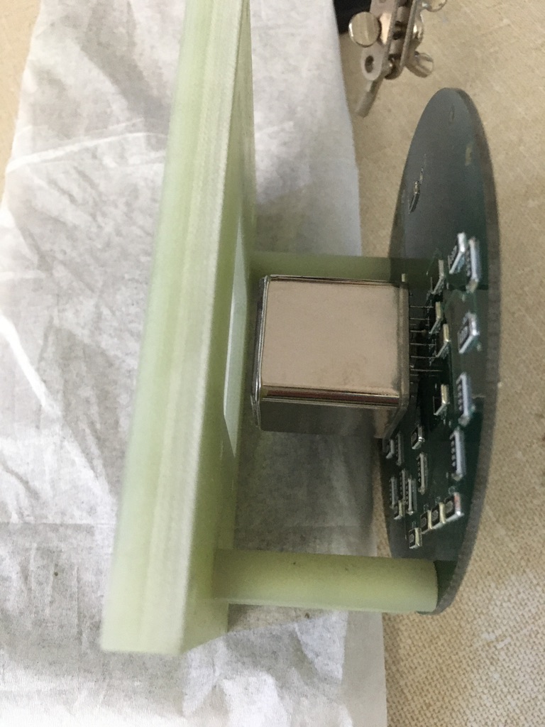
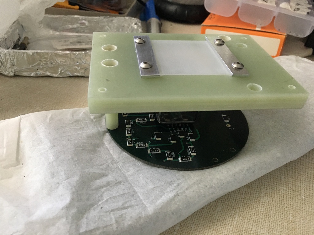
Figure 7.4: Two of the veto PMT assemblies constructed at MIT, including the 1-inch PMT, base circuit board, and TPB-coated acrylic window.

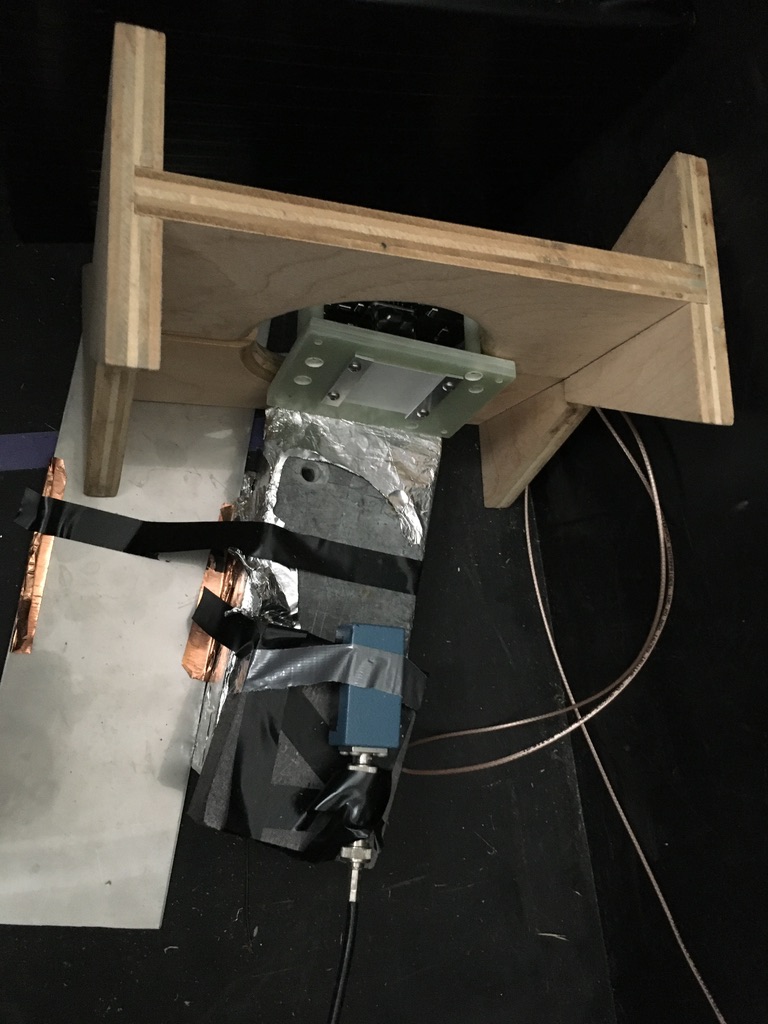
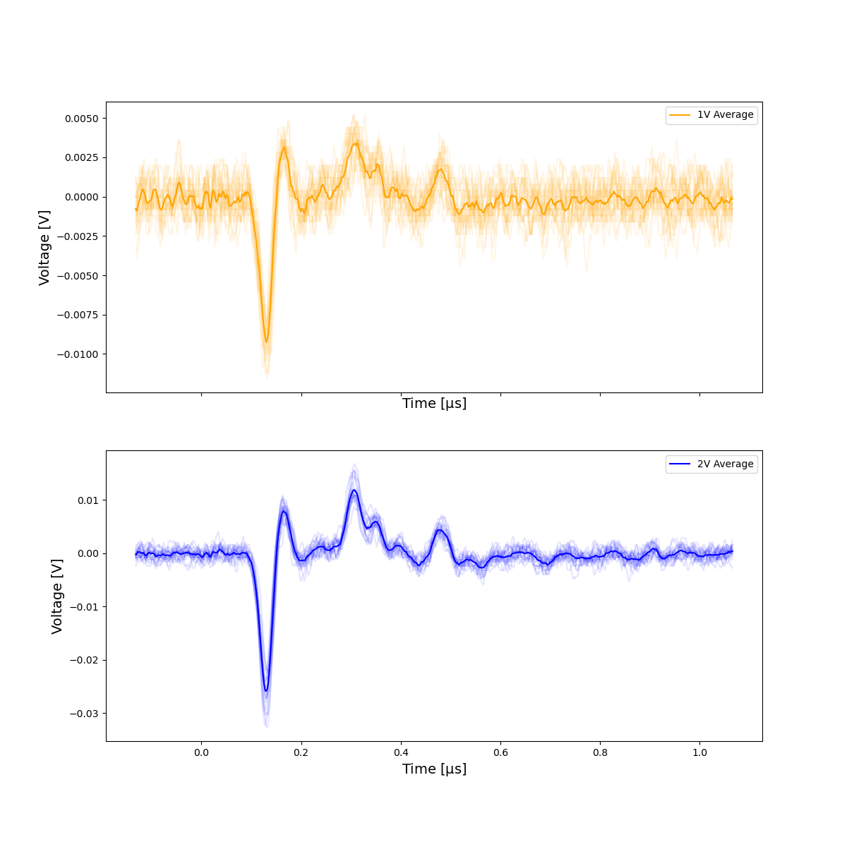
Figure 7.5: Figure 7.5 shows one of the veto PMTs across from the LED in the light-tight box. Figure 7.5 shows the average response of the 20 veto PMTs to 1 V (top) and 2 V (bottom) LED pulses.

CCM uses a variety of shielding between the target and detector to slow down and absorb beam-related neutrons, the most prominent beam-related background at the Lujan facility. This reduces the overall background rate and also separates beam-related neutrons in time from prompt BSM signals. Figure 7.2(b) shows the timing distributions of neutrons, $\pi^{+}$ decay-at-rest neutrinos, and prompt DM from the Lujan source after the 4 m of steel shielding surrounding the TMRS. The neutrons are pushed back further in time using additional shielding concrete, steel, and borated polyethylene shielding. For the CCM120 run, 6 ft of concrete and 16 in. of steel were placed immediately outside of the steel surrounding the TMRS. A 2 m-thick wall of steel was constructed in ER2, the room housing the CCM detector. Three additional walls of concrete bricks covered with borated polyethylene sheets were constructed around the front and sides of the CCM detector. The borated polyethylene sheets were included to absorb neutrons that had been sufficiently slowed down by the other shielding. An Eljen EJ-301 scintillation detector was deployed in a flight path neighboring CCM to observe the time of the prompt gamma flash from the Lujan source. Figure 7.6 shows the timing distribution of these photons compared to that of neutrons measured in the CCM120 detector. The discrepancy between these distributions was used to determine a 190 ns background-free region of interest (ROI) in which to look for prompt signals from neutrinos or BSM particles. The steady-state background expectation in the ROI is taken from a beam-out-of-time measurement before the ROI, which is about 22 times larger than the ROI itself [30].

A number of updates were made to the shielding for CCM200. A new larger wall of concrete, steel, and borated polyethylene was constructed in ER1, and more steel and concrete shielding was placed in ER2. Additionally, a steel and polyethylene roof was constructed over CCM to suppress backgrounds entering the detector from above. Preliminary estimates suggest the shielding upgrades have reduced backgrounds in CCM200 by a factor of 7 compared with CCM120 [275].

CCM uses three different methods to calibrate the detector. The first of these consists of two blue LEDs, which are used to determine the single photo-electron (p.e.) response of each PMT, as measured in units of analog-to-digital-conversion (ADC) counts. The PMTs are gain-matched in order to make the p.e.-to-ADC values as similar as possible between them. These LEDs are operated continuously while taking beam data in order to monitor changes in the single p.e. rate over time. CCM also uses ⁵⁷Co and ²²Na radioactive sources, which emit 126 keV and 2.2 MeV photons, respectively, to determine the energy scale of the detector. This is measured in units of p.e./MeVee (electromagnetic equivalent)–a quenching factor must be considered to determine the energy scale of the detector response to nuclear recoils [276, 277]. The sodium peak, which provided the more robust energy scale measurement, set the energy scale of CCM120 to $15.1\pm 4.0$ p.e./MeVee. Finally, a custom diode-pumped laser is used to determine the PMT response to 213 nm and 532 nm light. The ability to operate at two different wavelengths is important for disentangling the TPB response in CCM. Data from the radioactive sources and the laser were compared with output from a Geant4 simulation of CCM120 in order to tune the optical model of the detector, as described in Ref. [275].

During the operation of CCM120, the effective PMT quantum efficiency was about a factor of two lower than the expectation from Hamamatsu. This was likely related to the oxygen contamination, which was measured at the 2 ppm level in the CCM120 liquid argon. Such contamination can lead to a reduction of the scintillation light produced in liquid argon by about a factor of two [164], similar to the apparent reduction in quantum efficiency. In response to this, CCM200 will use a dedicated oxygen filtration system adapted from the Mini-CAPTAIN experiment [278] to keep the oxygen level below 100 ppb. Filtration is expected to increase the scintillation light output by a factor of around three [275].

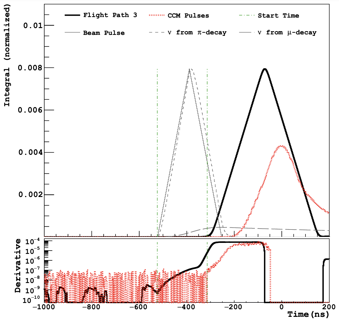
Figure 7.6: The timing distribution of photons from the Lujan source (solid black line) compared with that of neutrons measured in CCM120 (dashed red line). Figure from Ref. [30].

7.2 Cherenkov Light Reconstruction

CCM relies predominantly on scintillation light to reconstruct particle interactions in the detector. This is because liquid argon is a powerful scintillation medium, as described in section 3.1.3. That being said, the identification of Cherenkov radiation in CCM is a promising potential upgrade. Cherenkov radiation refers to the light emitted by a charged particle as it travels faster than the speed of light in a given medium [279]. The particle polarizes surrounding atoms as it moves through the material, creating a cloud of electric dipoles. If $\beta>c/n$ (where $n$ is the wavelength-dependent index of refraction), the dipoles are not arranged symmetrically around the particle, resulting in a non-vanishing overall dipole moment. The time variation of this dipole moment results in Cherenkov radiation. The light is emitted in a cone with an opening angle of $\cos\theta_{C}=1/n\beta$. The number of photons emitted per unit length is given by [279]

$$\frac{dN}{dx}=2\pi\alpha z^{2}\int_{\lambda_{1}}^{\lambda_{2}}\bigg{(}1-\frac{1}{(n(\lambda)\beta)^{2}}\bigg{)}\frac{d\lambda}{\lambda^{2}},$$ (7.1)

where $z$ is the electric charge of the particle in units of the electron charge $e$, and $\lambda_{1}$ and $\lambda_{2}$ represent the photon wavelength range under consideration. From equation 7.1, one can see that the intensity of Cherenkov radiation peaks at lower wavelengths.

For liquid argon, $n(\lambda=128~{}{\rm nm})\sim 1.5$ and decreases for larger wavelengths [167]. This means that only electrons satisfy the $\beta>c/n$ requirement at typical CCM energies of $\mathcal{O}(10~{}{\rm MeV})$. Though they are neutral, photons in this energy regime will produce Cherenkov light after undergoing pair production to an $e^{+}e^{-}$ final state. Crossing cosmic muons will also produce Cherenkov light, though such events are rare in the 1.6 $\mu$s beam window and can be tagged by the veto region. Importantly, the most prominent backgrounds in CCM–beam-related neutrons and low-energy photons from radioactive impurities–will not produce Cherenkov light. In contrast, signals from ALPs [271] and other BSM scenarios of interest to CCM [145] will produce Cherenkov light via higher-energy electrons and photons in the final state. Thus, Cherenkov light identification is a promising method for rejecting backgrounds in CCM and maximizing sensitivity to new physics. The directional nature of Cherenkov light will also be helpful in requiring particles to originate from the tungsten target, which is not possible using only isotropic scintillation light.

In order to determine the number of Cherenkov photons generated per unit length traveled by a charged particle, one must perform the integration equation 7.1. To do this, we use the parameterization of the liquid argon index of refraction given in Ref. [167]. We fix $\lambda_{2}=700~{}{\rm nm}$, as this is the upper bound on the detectable wavelength range of the CCM PMTs. Figure 7.7(a) shows a numerical integration of equation 7.1 for an electron ($z=1$) as a function of $\lambda_{1}$. One can see that sensitivity to lower wavelengths greatly increases the number of photons one can detect. This is possible in CCM thanks to the use of TPB, which can covert the UV Cherenkov light into the visible range, greatly increasing the number of Cherenkov photons detected by each PMT. The cone angle as a function of the electron kinetic energy and photon wavelength is shown in figure 7.7(b), which is $\cos\theta_{C}\approx 0.8$ over most of the parameter space. This figure also indicates the threshold for Cherenkov emission; over most photon wavelengths, Cherenkov light is produced for electron kinetic energies above $T_{e^{-}}\sim 0.4~{}{\rm MeV}$.

A number of specialized studies have been performed investigating the detection of Cherenkov light in scintillation detector mediums, including water-based liquid scintillator [280, 281], slow-fluor scintillator [282], and linear alkylbenzene [283]. Two full-scale experiments have been able to perform a statistical measurement of Cherenkov radiation in a scintillating medium: Borexino, observing elastic scattering of sub-MeV solar $\nu_{e}$ in a large liquid scintillator detector [284], and ICARUS, observing cosmic muons in a large liquid argon detector [285]. However, no large-scale scintillation experiment has been able to observe Cherenkov light on an event-by-event basis. This is because the Cherenkov light output is typically smaller than the scintillation light output by around two orders of magnitude, which can be understood by comparing the numbers in figure 7.7(a) to the $\mathcal{O}(10^{4})$ scintillation photons per MeV produced in liquid argon [158].

Event-by-event detection of Cherenkov light might be possible in CCM for a few reasons. First, liquid argon is transparent to UV light, which substantially increases the number of detectable Cherenkov photons as shown in figure 7.7(a). TPB-coated PMTs can detect these UV Cherenkov photons by shifting them into the visible range. The wavelength-shifting efficiency of TPB actually increases by a factor of around two for $\lambda\sim 200~{}{\rm nm}$ compared to 128 nm argon scintillation light [286], potentially boosting the response of CCM PMTs to Cherenkov light. Second, the singlet lifetime of argon excimers is approximately 8 ns [160], which is much slower than the Cherenkov light emission timescale ($<1~{}{\rm ns}$) [287]. The 2 ns sampling time of the CCM digitizers may allow for the separation in time of prompt Cherenkov photons from the first scintillation photons. Finally, 20% of the PMTs in CCM are not coated in TPB. This means they are only sensitive to scintillation photons after they have been emitted from TPB somewhere else in the detector, delaying their arrival time in these PMTs. In contrast, Cherenkov photons in the visible regime will indeed produce signals on the uncoated PMTs. Though the larger UV component of the Cherenkov spectrum will not be accessible, even just a few photoelectrons detected by uncoated PMTs in the prompt time region would be a strong indication of Cherenkov light.

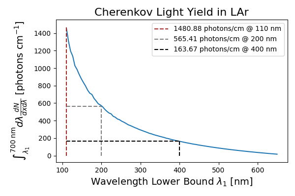
(a)

(b)

Figure 7.7: Figure 7.7(a) shows the integration in equation 7.1 as a function of $\lambda_{1}$ for $\lambda_{2}=700~{}{\rm nm}$ and $z=1$. Figure 7.7(b) shows the Cherenkov cone angle $\cos\theta_{C}$ for an electron as a function of the photon wavelength and the electron kinetic energy.

7.2.1 Simulation-Based Sensitivity Estimation

In order to assess the sensitivity of CCM to Cherenkov light, we use the Geant4 simulation of CCM200 described in Ref. [275]. We inject electrons at the center of the detector, traveling along the beam direction with kinetic energies of $\{1,2,3,4,5\}~{}{\rm MeV}$. In addition to the usual scintillation light, Cherenkov light is emitted along the electron path within the 100 nm to 700 nm wavelength range. Both scintillation and Cherenkov photons are subject to wavelength-dependent effects within the detector, including absorption by impurities [164, 165] and Rayleigh scattering [167]. The TPB response in the simulation has not been carefully evaluated in the $200\leq\lambda~{}[{\rm nm}]\leq 400$ regime, so we have turned the TPB off for the purposes of this study. Instead, we apply a time offset for coated PMTs reflecting the TPB emission, which is sampled from an exponential with a time constant of 1.7 ns [288]. For both coated and uncoated PMTs, we apply an additional time offset related to the rise time of the PMT $\tau_{\rm PMT}$, which is about 2.5 ns in CCM. This is sampled from a Gaussian with a mean and width of $\tau_{\rm PMT}/2$. For each photon that hits a PMT surface, we apply a weight reflecting the detection probability $P_{\rm det}$, which is calculated as

$$\begin{split}&P_{\rm det}^{\rm uncoated}=P_{\rm PMT}\\ &P_{\rm det}^{\rm coated}=P_{\rm PMT}P_{\rm TPB},\end{split}$$ (7.2)

where $P_{\rm PMT}$ reflects the PMT quantum efficiency and $P_{\rm TPB}$ reflects the impact of TPB absorption and re-emission on the detection probability. The former is given by $P_{\rm PMT}=0.15$ for coated PMTs and

$$P_{\rm PMT}=\begin{cases}0.15&300<\lambda~{}[{\rm nm}]<650\\ 0&{\rm otherwise}\end{cases}$$ (7.3)

for uncoated PMTs, where $0.15$ is the typical quantum efficiency of a cryogenic PMT [275, 289]. This reflects the approximation that TPB makes the coated PMTs sensitive to all photon wavelengths within 100 nm to 700 nm, while the uncoated PMTs are only sensitive to the visible range [289]. The TPB transmission probability is approximated by

$$\begin{split}&P_{\rm TPB}=P_{\rm abs}P_{\rm geo}P_{\rm vis},\\ &P_{\rm abs}=\begin{cases}0.4&\lambda<200~{}{\rm nm}\\ 0.66&\lambda>200~{}{\rm nm}\\ \end{cases},\\ &P_{\rm geo}=0.4,\\ &P_{\rm vis}=\begin{cases}1.0&\lambda<400~{}{\rm nm}\\ 0.8&\lambda>400~{}{\rm nm}\\ \end{cases},\\ \end{split}$$ (7.4)

where $P_{\rm abs}$ is a simple step function representation of the TPB absorption efficiency [286], $P_{\rm geo}$ is a geometric efficiency reflecting the fact that TPB emits photons isotropically off of the hemispherical PMT surface, and $P_{\rm vis}$ reflects the tendency of TPB to absorb visible light to some degree, as evidenced by its cloudy nature.

Using the setup described above, we simulate $10^{4}$ electrons for each of the five tested kinetic energies to generate average templates of the expected number of registered hits in each PMT. In figure 7.8 we show templates for electrons with kinetic energies of $T_{e^{-}}=1~{}{\rm MeV}$ and $T_{e^{-}}=5~{}{\rm MeV}$. Separate templates are shown including all photons and only scintillation photons (i.e., without Cherenkov light). The positions of each PMT here can be thought of as an unfolding of the cylindrical CCM detector, where the center of the image ($(x,y)=(0,0)$ in the middle panel) corresponds to the beam direction. Note that these templates only consider the first 8 ns after the electron starts traveling through the detector, as this is the region in which we expect Cherenkov light to stand out over scintillation light. This is indeed the case; the PMTs in figures 7.8(a) and 7.8(c) see much more light than those in figures 7.8(b) and 7.8(d). This is especially true of the uncoated PMTs (dashed circles), which do not suffer the TPB detection inefficiency captured by equation 7.4 nor the time delay from TPB re-emission. The separation between the templates with and without Chernekov light is more obvious for $T_{e^{-}}=5~{}{\rm MeV}$ than for $T_{e^{-}}=1~{}{\rm MeV}$, indicating that Chernekov light will be a stronger discriminator in the higher energy region. The directional nature of Cherenkov light is also clear here. While scintillation photons are more-or-less isotropic, the event displays with Cherenkov photons included clearly show detected p.e. clustered around the beam direction. Figure 7.9 shows example event displays of the number of p.e. detected in each CCM PMT in a single simulated electron event for both $T_{e^{-}}=1~{}{\rm MeV}$ and $T_{e^{-}}=5~{}{\rm MeV}$.

We use these simulations to build up a template-based Poisson likelihood reflecting the probability that a given event does or does not contain scintillation light. We evaluate a separate Poisson likelihood in each PMT across five time bins of 2 ns width each, which reflects the temporal sampling rate in CCM. The total likelihood is given by

$$\mathcal{L}_{\rm all/scint}=\prod_{\rm PMTs~{}i}\prod_{\rm time~{}bins~{}j}P_{\rm Poisson}(k_{ij}|\mu^{\rm all/scint}_{ij}),$$ (7.5)

where $P_{\rm Poisson}$ is the Poisson probability, $k_{ij}$ is the observed number of p.e. in PMT $i$ and time bin $j$, and $\mu^{\rm all}_{ij}$ ($\mu^{\rm scint}_{ij}$) is the prediction for the templates with (without) Cherenkov light, as shown in figure 7.8. In the case that no events are predicted in a given PMT $i$ and time bin $j$, we set $\mu_{ij}=10^{-4}$, reflecting an uncertainty of one event over the $10^{4}$ simulations. We can then use the detected p.e. in each simulation to build distributions of the log-likelihood-ratio test statistic

$$\Delta\log\mathcal{L}\equiv\log\mathcal{L}_{\rm all}-\log\mathcal{L}_{\rm scint}.$$ (7.6)

In figure 7.10 we show distributions of this test statistic for $T_{e^{-}}=1~{}{\rm MeV}$ and $T_{e^{-}}=5~{}{\rm MeV}$, both with and without Cherenkov light. Given the overall sign of equation 7.6, $\Delta\log\mathcal{L}$ is larger when Cherenkov photons are included. This can be seen in figure 7.10, as the distributions with Cherenkov photons included sit at higher values of $\Delta\log\mathcal{L}$ compared to those without Cherenkov photons. The vertical line in this plot indicates the lower bound on $\Delta\log\mathcal{L}$ that can reject 99% of scintillation-only backgrounds, which can be thought of as, for example, beam-related neutrons depositing as many scintillation photons as an electron with the specified kinetic energy. Figure 7.11 shows curves of the efficiency to retain events with Cherenkov rings v.s. the rejection factor for events without Cherenkov rings, which are obtained by considering successively larger lower bounds on $\Delta\log\mathcal{L}$. In the $T_{e^{-}}=5~{}{\rm MeV}$ case, one can achieve a background rejection of $0.99$ while retaining a signal efficiency of $0.99$–thus, a Cherenkov likelihood cut has the potential to reduce backgrounds by around two orders of magnitude for free.

Of course, a few caveats must be mentioned regarding this study. Most importantly, we have only constructed a likelihood for electrons of a few example kinetic energies originating at the center of the detector and traveling along the beam direction. A full Cherenkov likelihood will need to be a function of the particle vertex $(x,y,z)$ and direction $(\theta,\phi)$ in addition to the particle energy. In order to properly assess the background rejection power of a Cherenkov-based cut, one will need to simulate neutrons in CCM using a realistic flux from the Lujan target after moderation by the CCM shielding. Finally, a more realistic TPB model within Geant4 itself will allow for a more robust prediction of the difference in coated and uncoated PMT response to Chernekov light. That being said, the results from this simulation study indicate the power of a Cherenkov reconstruction algorithm in CCM and suggest that such a reconstruction is feasible for electrons with energies of a few MeV or greater. Angular cuts based on the reconstructed direction of the Cherenkov cone will help further reduce backgrounds by correlating events with the beam direction.

(a) With Cherenkov photons; $T_{e^{-}}=1~{}{\rm MeV}$

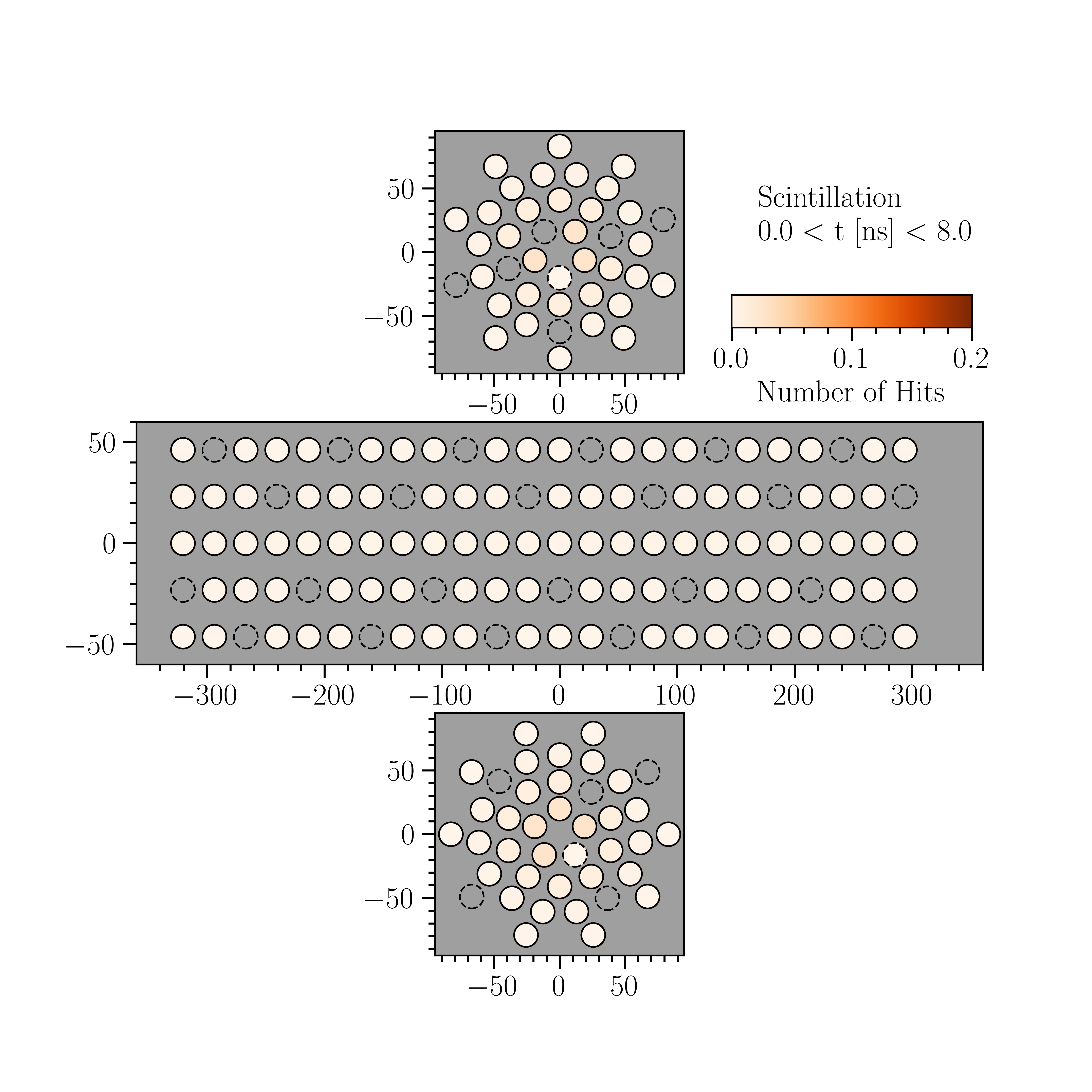
(b) Without Cherenkov photons; $T_{e^{-}}=1~{}{\rm MeV}$

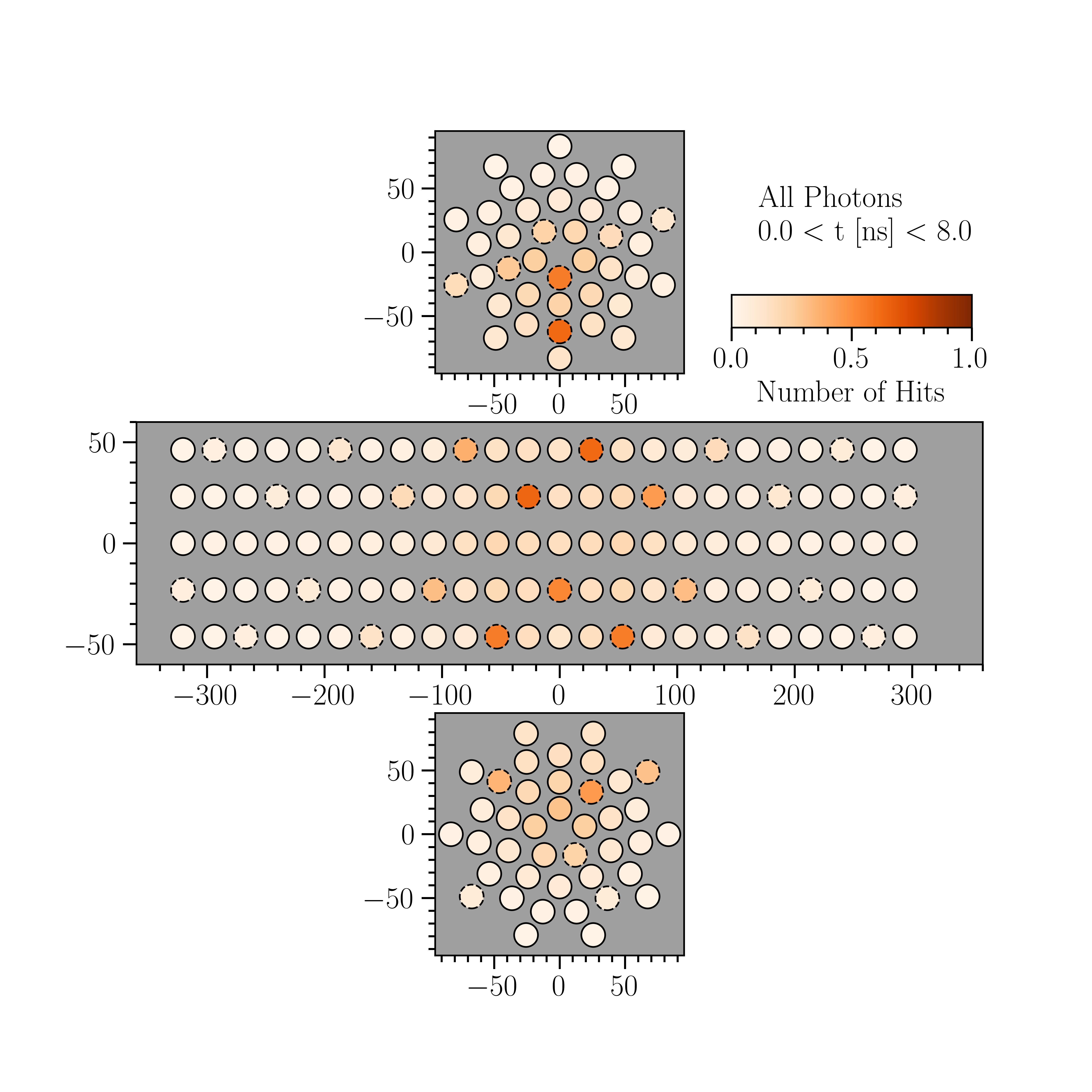
(c) With Cherenkov photons; $T_{e^{-}}=5~{}{\rm MeV}$

(d) Without Cherenkov photons; $T_{e^{-}}=5~{}{\rm MeV}$

Figure 7.8: Templates of the average number of p.e. detected in each CCM PMT within the first 8 ns of an electron event. Different templates are shown for electron kinetic energies of $T_{e^{-}}=1~{}{\rm MeV}$ and $T_{e^{-}}=5~{}{\rm MeV}$, both with and without Cherenkov photons. Coated (uncoated) PMTs are indicated by the solid (dashed) circles. Grey PMTs indicate those which registered no hits within the first 8 ns across all simulations. The dimensions on each axis are in units of cm.

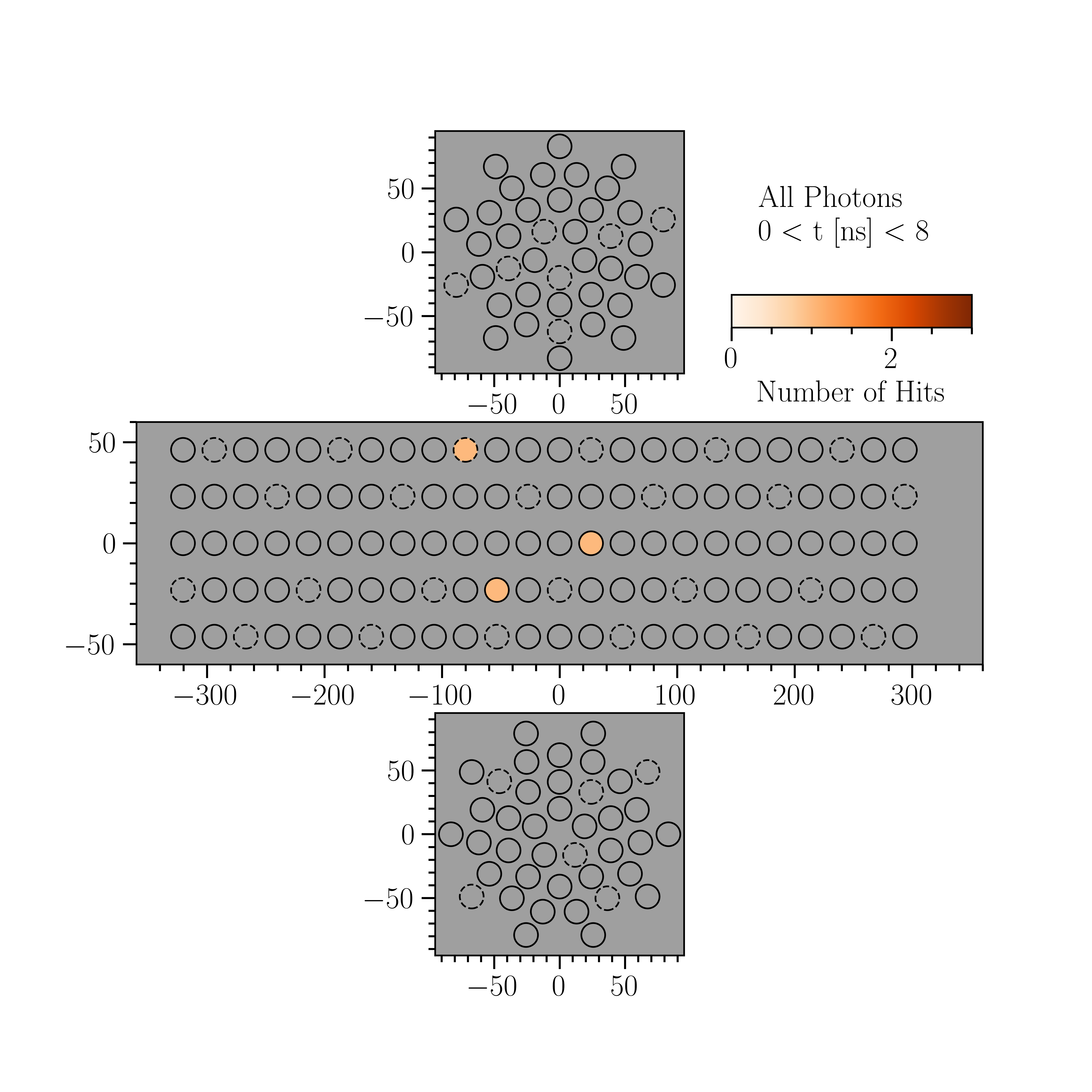
(a) $T_{e^{-}}=1~{}{\rm MeV}$

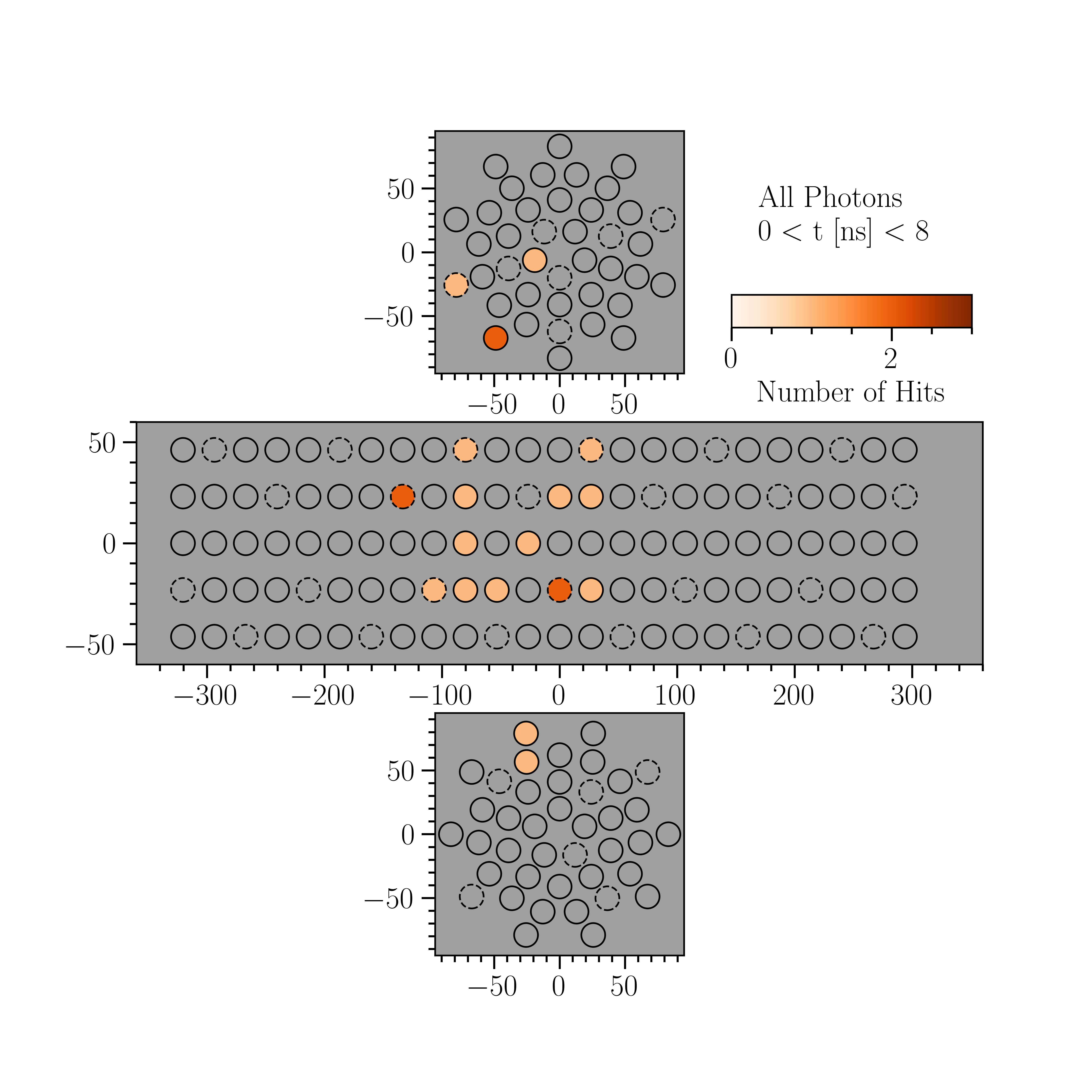
(b) $T_{e^{-}}=5~{}{\rm MeV}$

Figure 7.9: Example event displays showing the total number of p.e. detected in each CCM PMT within the first 8 ns of a single simulated electron event. Displays are shown for electron kinetic energies of $T_{e^{-}}=1~{}{\rm MeV}$ and $T_{e^{-}}=5~{}{\rm MeV}$. Coated (uncoated) PMTs are indicated by the solid (dashed) circles. Grey PMTs indicate those which registered no hits in the first 8 ns of this specific simulation.

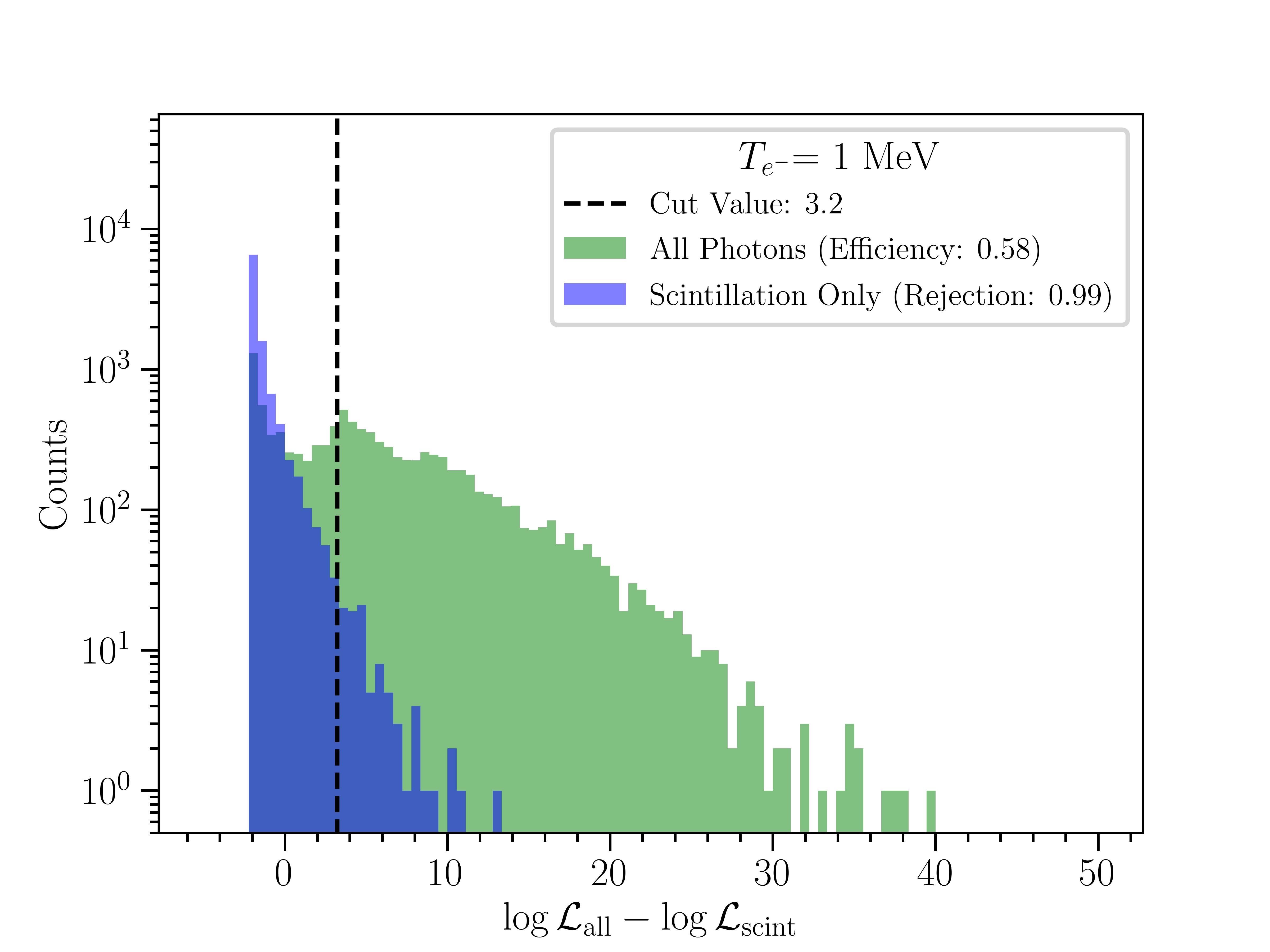
(a) $T_{e^{-}}=1~{}{\rm MeV}$

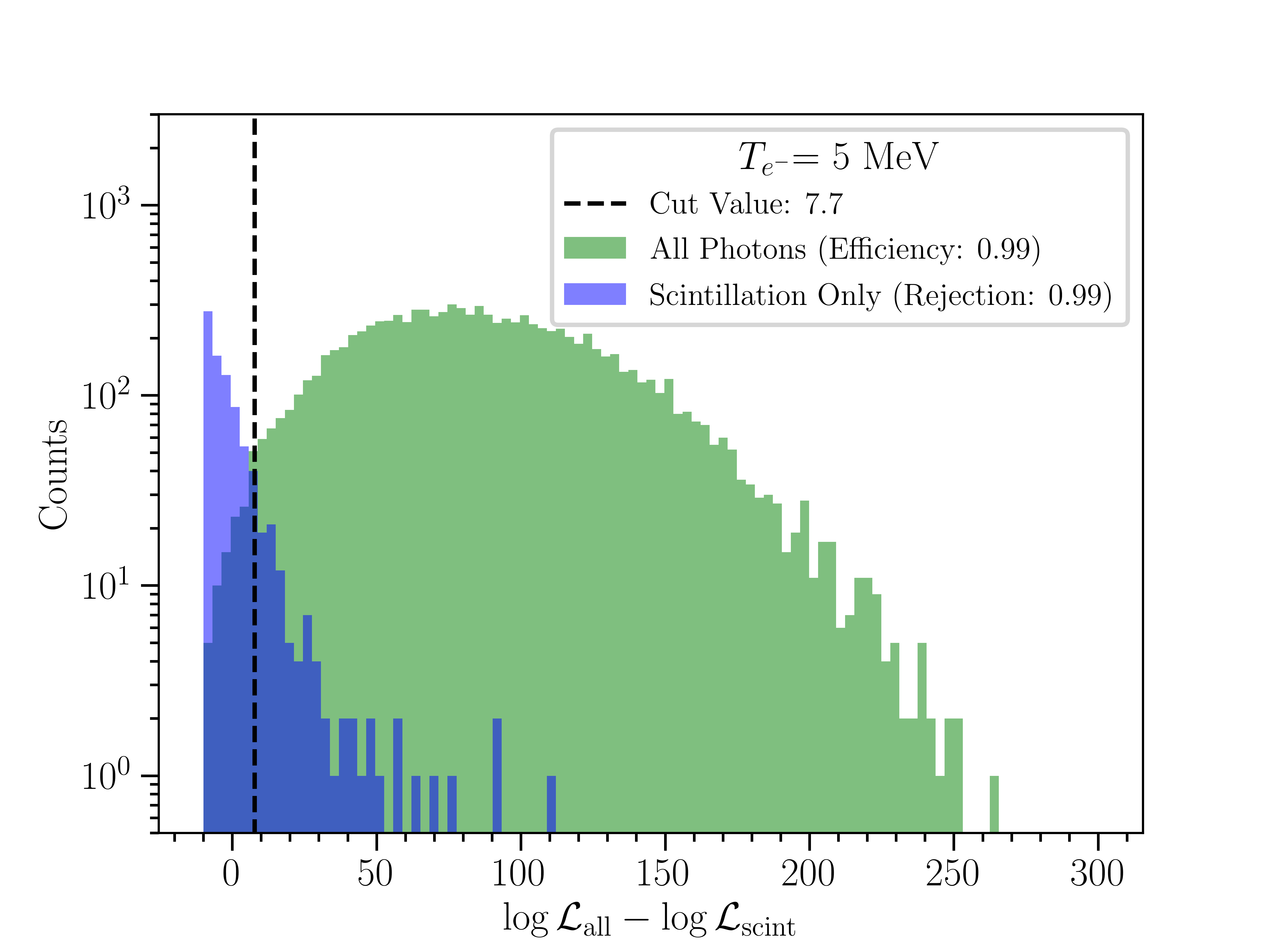
(b) $T_{e^{-}}=5~{}{\rm MeV}$

Figure 7.10: Distributions of the test statistic in equation 7.6 over all $10^{4}$ simulations, considering either all photons or scintillation photons only. Distributions are shown for $T_{e^{-}}=1~{}{\rm MeV}$ and $T_{e^{-}}=5~{}{\rm MeV}$. The vertical line indicates the lower bound requirement which can reject 99% of scintillation-only backgrounds.

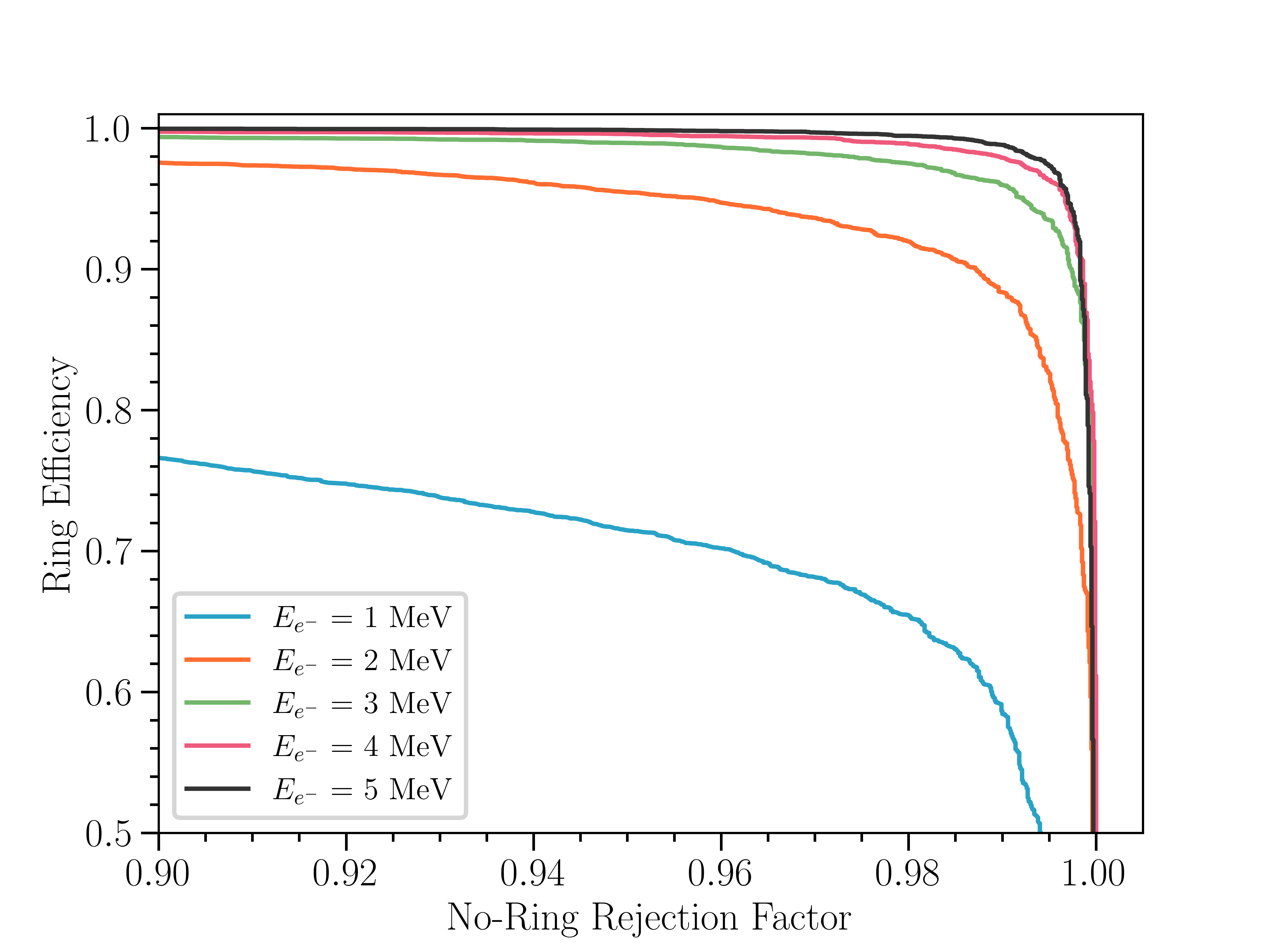
Figure 7.11: Curves of the efficiency to retain events with Cherenkov light (“Ring efficiency”) v.s. the fraction of events without Cherenkov light that can be rejected (“No-Ring Rejection Factor”), generated by considering successively larger lower bounds on $\Delta\log\mathcal{L}$. Different curves are shown for $T_{e^{-}}\in\{1,2,3,4,5\}~{}{\rm MeV}$.

7.2.2 Identifying Cherenkov Light in Data

Having established the feasibility of a dedicated Cherenkov light reconstruction, we now discuss the path toward realizing this in CCM data. Cherenkov reconstruction requires a more detailed treatment of the timing information contained in PMT signals. The existing CCM reconstruction uses exponential smoothing, averaging, and derivative filters to determine regions of each PMT waveform with potential activity. A pulse is defined as a region in which the derivative goes below a given negative threshold, then becomes positive, then relaxes below the positive threshold, as shown in figure 7.12(a). Figure 7.12(b) shows the identified pulses in an example CCM120 data event using this technique. Each pulse is then approximated by a triangle with a length and height given by the pulse length and absolute value of the integral of the waveform derivative over the pulse, respectively. Pulses were further required to be at least 20 ns in length to reduce the impact of noise. While this method was sufficient for the scintillation-based CCM120 analyses, which were mainly concerned with the many-p.e. scintillation pulse summed over all PMTs, identification of Cherenkov light will require a new pulse-finding algorithm that treats single p.e. pulses more carefully. It must also be able to retain pulses shorter than 20 ns to be sensitive to the Cherenkov-dominated early time window studied in section 7.2.1.

To address these issues, we have begun revamping the pulse-finding algorithm in preparation for CCM200. This includes the use of a more realistic single p.e. template to replace the triangle approximation. We use a parameterization of the single p.e. waveform based on that used by the IceCube collaboration [290],

$$w(t)=\frac{c}{[e^{-(t-t_{0})/b_{1}}+e^{(t-t_{0})/b_{2}}]^{8}},$$ (7.7)

where $c$, $t_{0}$, $b_{1}$ and $b_{2}$ are free parameters to be fit using data. To determine the best-fit single p.e. template for each PMT, we begin by isolating candidate pulses using the derivative filter in figure 7.12(a). We restrict to candidate pulses with an amplitude between 20 and 40 ADC counts, which corresponds roughly to the single p.e. amplitude range in CCM. We fix two of the template parameters using the observed peak amplitude $w_{\rm max}$ and peak time $t_{\rm max}$ for each candidate pulse,

$$\begin{split}&w_{\rm max}=\frac{c}{\Big{[}\Big{(}\frac{b_{1}}{b_{2}}\Big{)}^{\frac{b_{2}}{b_{1}+b_{2}}}+\Big{(}\frac{b_{2}}{b_{1}}\Big{)}^{\frac{b_{1}}{b_{1}+b_{2}}}\Big{]}^{8}},\\ &t_{\rm max}=t_{0}+\frac{b_{1}b_{2}}{b_{1}+b_{+}2}\ln(b_{2}/b_{1}).\\ \end{split}$$ (7.8)

Figure 7.13 shows the result of this template fit for candidate pulses on two different PMTs in CCM200 beam data. The next step is to determine a robust single p.e. template for each PMT in CCM200. These templates can then be used to unfold the observed waveform on every PMT for a given event into a series of single p.e. pulses at different times and with different amplitudes. Such a reconstruction will help pick out an excess of single p.e. pulses in the early time window, which would be an indication of Cherenkov light.

In order to inform the development of our Cherenkov reconstruction, we have isolated a new data sample in CCM200: cosmic muons. These are useful for two reasons: (1) downward-going cosmic muons will produce Cherenkov light along a known direction, and (2) isotropic emission of Michel electrons from muon decay-at-rest will help test the angular resolution of the Cherenkov reconstruction. Michel electrons can also serve as an important calibration point for the scintillation-based energy reconstruction, as they are emitted with a known energy distribution peaking at $m_{\mu}/2$ [172]. To tag cosmic muons, we have assembled six pairs of CosmicWatch detectors [291] on top of CCM. Each detector consists of a piece of plastic scintillator and a silicon photomultiplier, which detects photons produced in the scintillator. Two detectors can be stacked on top of one another and set to trigger on the coincident observation of light between the pair, indicative of a crossing cosmic muon. Figure 7.14(a) shows an image of the six CosmicWatch pairs on top of CCM. The detectors in each pair are separated by approximately 6 in. of foam to ensure that crossing cosmic muons are sufficiently downward-going to pass through the bottom of the detector. We have set up a dedicated cosmic muon trigger in CCM200 that saves an event whenever any of the six CosmicWatch pairs on top of CCM register a coincident signal. A diagram of this trigger is shown in figure 7.14.

The cosmic muon trigger became operational in Summer 2022 and can run concurrently with the beam, strobe, and LED triggers. The total trigger rate is a bit under 1 Hz, meaning that $\mathcal{O}(10^{6})$ cosmic muons have already been collected over the first few months of CCM200 data. Figure 7.15(a) shows the summed waveform across all PMTs in CCM200 for a single cosmic muon trigger. One can also see a delayed signal from what is likely a Michel electron. Though we are still in the preliminary phase of analyzing data from the cosmic muon trigger, we touch briefly on a promising initial study of this dataset. This analysis examines the summed waveform in coated and uncoated PMTs separately in the top half and bottom half of the barrel of the detector. We look specifically at the initial rise time $t_{0}$ of each summed waveform, defined as the time tick at which the waveform passes 0.5% of its maximum value. In the scintillation only case, the coated PMTs should see a signal earlier than the uncoated PMTs ($t_{0}^{\rm coated}<t_{0}^{\rm uncoated}$), as only photons reflected from elsewhere in the detector will register a p.e. on the uncoated PMTs. This difference should diminish when Cherenkov light is involved, as both coated and uncoated PMTs will observe Cherenkov light to some level. We set the threshold to 0.5% as this reflects roughly the total number of Cherenkov photons generated by a crossing cosmic muon compared to scintillation photons. Figure 7.15 shows the distribution of $t_{0}^{\rm coated}-t_{0}^{\rm uncoated}$ for PMTs in the top and bottom of the barrel over $\sim 75$ cosmic muon events. Given the angle of the Chernekov cone emitted by a cosmic muon traveling downward along the central axis of the detector, only PMTs in the bottom half of the barrel will observe Cherenkov light. This is consistent with the distributions in figure 7.15–the PMTs in the upper half of the barrel peak at $t_{0}^{\rm coated}-t_{0}^{\rm uncoated}\sim-5~{}{\rm ns}$, while PMTs in the lower half of the barrel peak around zero. Thus, the delay of the signal in uncoated PMTs appears to disappear for PMTs sensitive to Cherenkov light. This is far from a definitive detection of Cherenkov light in the CCM detector, as one would need to carefully consider geometric effects in the CCM detector to predict $t_{0}^{\rm coated}-t_{0}^{\rm uncoated}$ distributions with and without Cherenkov light. However, it is a promising initial indication that Cherenkov reconstruction might be possible in CCM by leveraging differences in the coated and uncoated PMT signals.

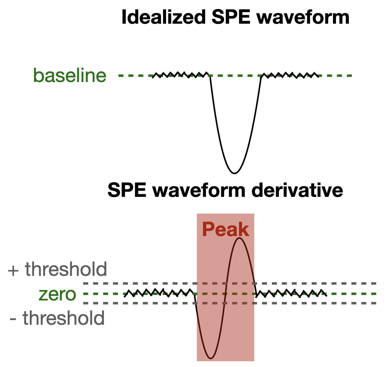
(a)

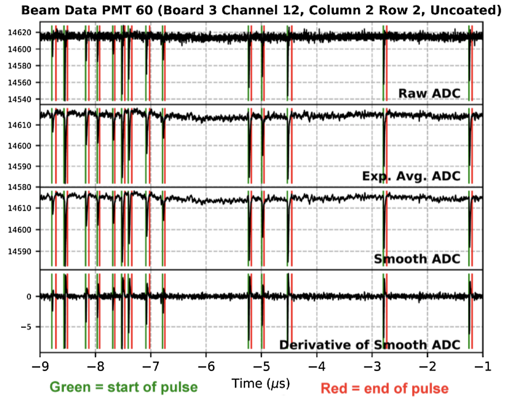
(b)

Figure 7.12: Figure 7.12(a) shows a schematic depiction of the derivative-based pulse definition in the current CCM reconstruction. Figure 7.12(b) shows an example of this pulse finder in a data event, from Ref. [30].

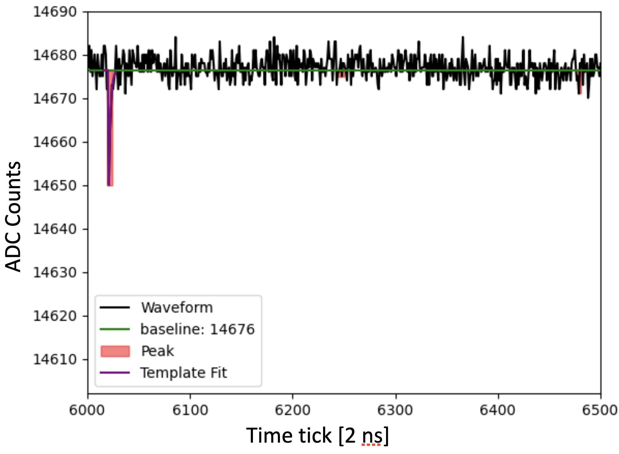
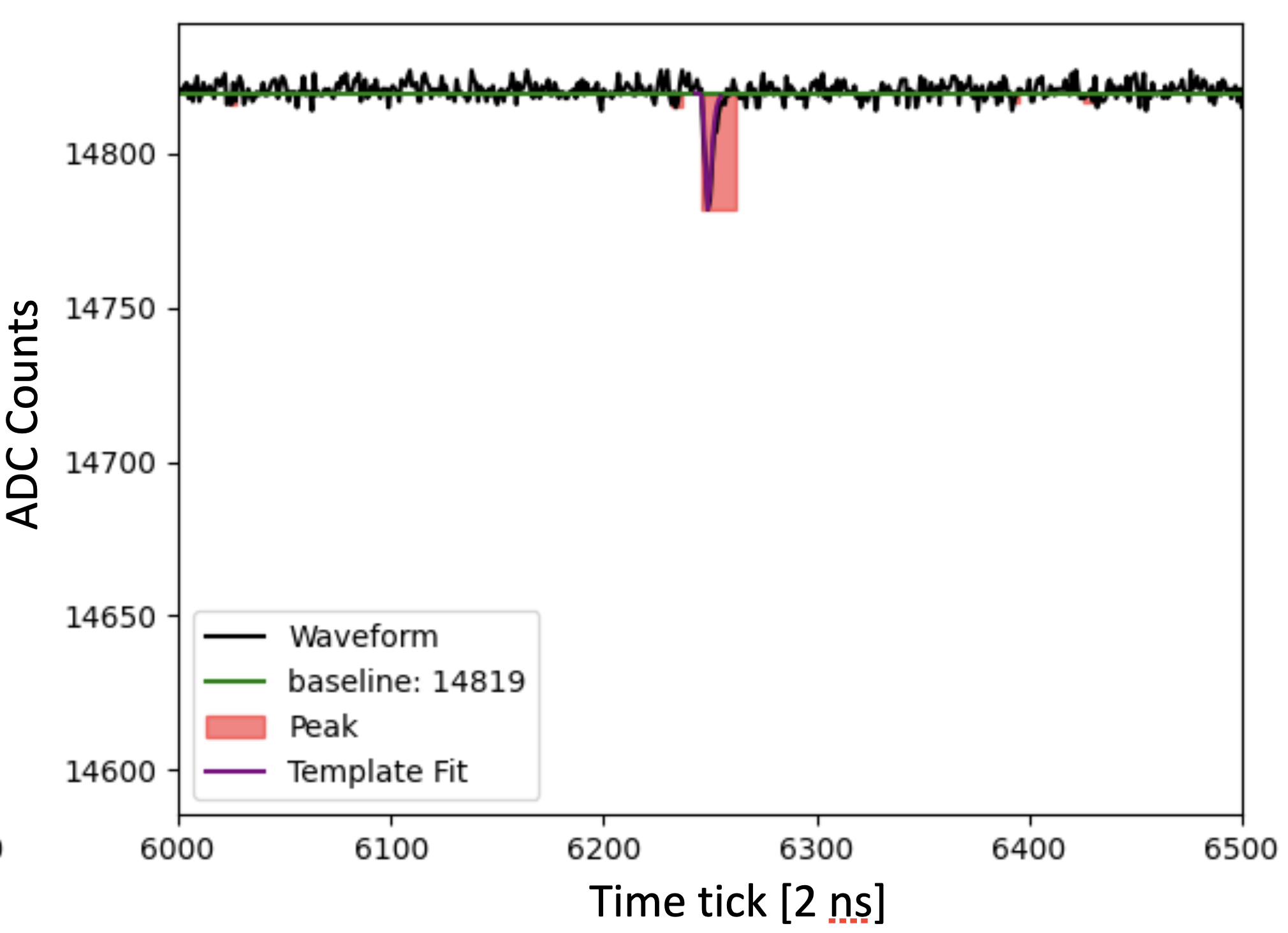
Figure 7.13: Two example waveforms from CCM200 beam data. The regions identified by the derivative filter are indicated in red and the result of the fit to equation 7.7 is indicated by the purple curves.

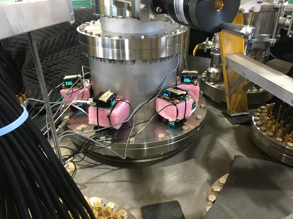
(a)

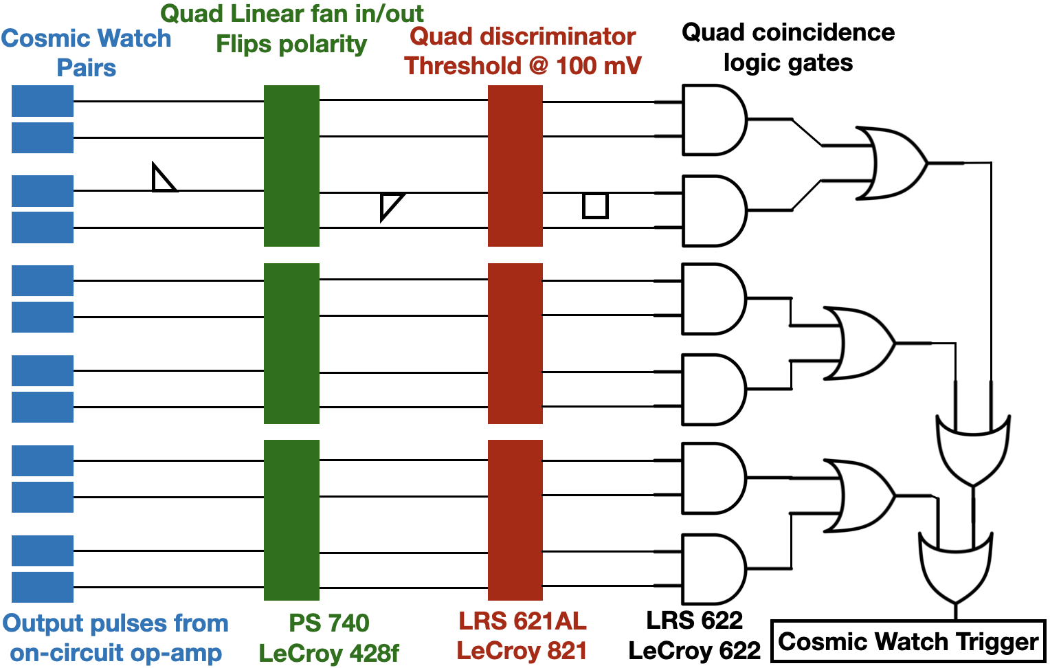
Figure 7.14: Figure 7.14(a) shows an image of the six CosmicWatch pairs on top of the CCM detector. Figure 7.14 shows a schematic diagram of the cosmic muon trigger in CCM200.

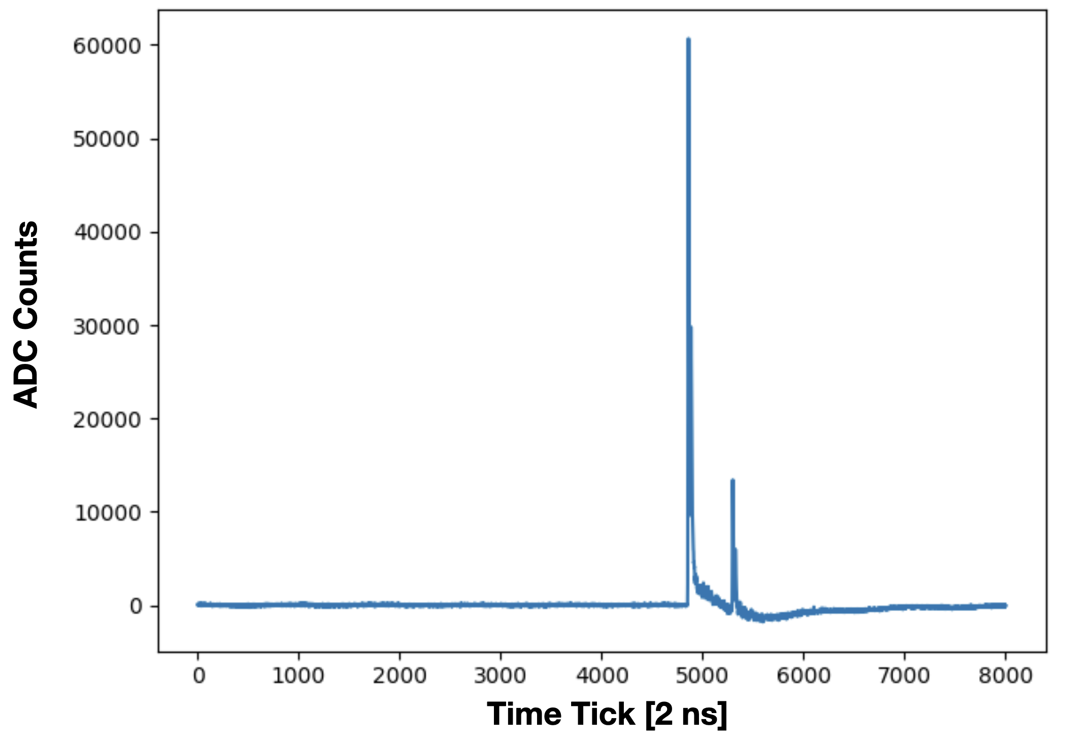
(a)

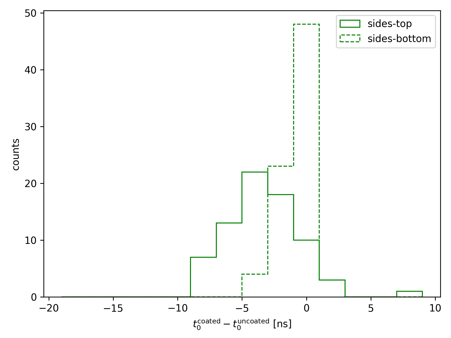
Figure 7.15: Figure 7.15(a) shows the summed waveform across all PMTs in CCM for a single example cosmic muon trigger. The delayed signal from a Michel electron can also be seen. Figure 7.15 shows the difference in rise times between coated and uncoated PMT signals in the top and bottom halves of the barrel of the detector (labeled “sides-top” and “sides-bottom”, respectively), as described in the text.

7.3 Neutrissimos in CCM

We close our CCM discussion with an investigation of the sensitivity of CCM200 to the neutrissimo model of chapter 6. The idea of looking for dipole-coupled HNLs at CE$\nu$NS experiments has already been proposed in the literature [236]. The low energy threshold of these experiments enables a powerful signal definition: the coincidence of a nuclear recoil from upscattering ($\nu A\to\mathcal{N}A$) followed by a higher energy photon from neutrissimo decay ($\mathcal{N}\to\nu\gamma$). In particular, the upcoming NUCLEUS experiment is projected to have strong sensitivity to $d_{e\mathcal{N}}$ for $m_{\mathcal{N}}\lesssim 10~{}{\rm MeV}$ [236]. In this section, we investigate whether CCM200 might also have sensitivity to neutrissimos in the $m_{\mathcal{N}}=\mathcal{O}(10~{}{\rm MeV})$ regime. The important advantage of CCM200 is that it is already running; projected sensitivities derived here will become limits within a few years.

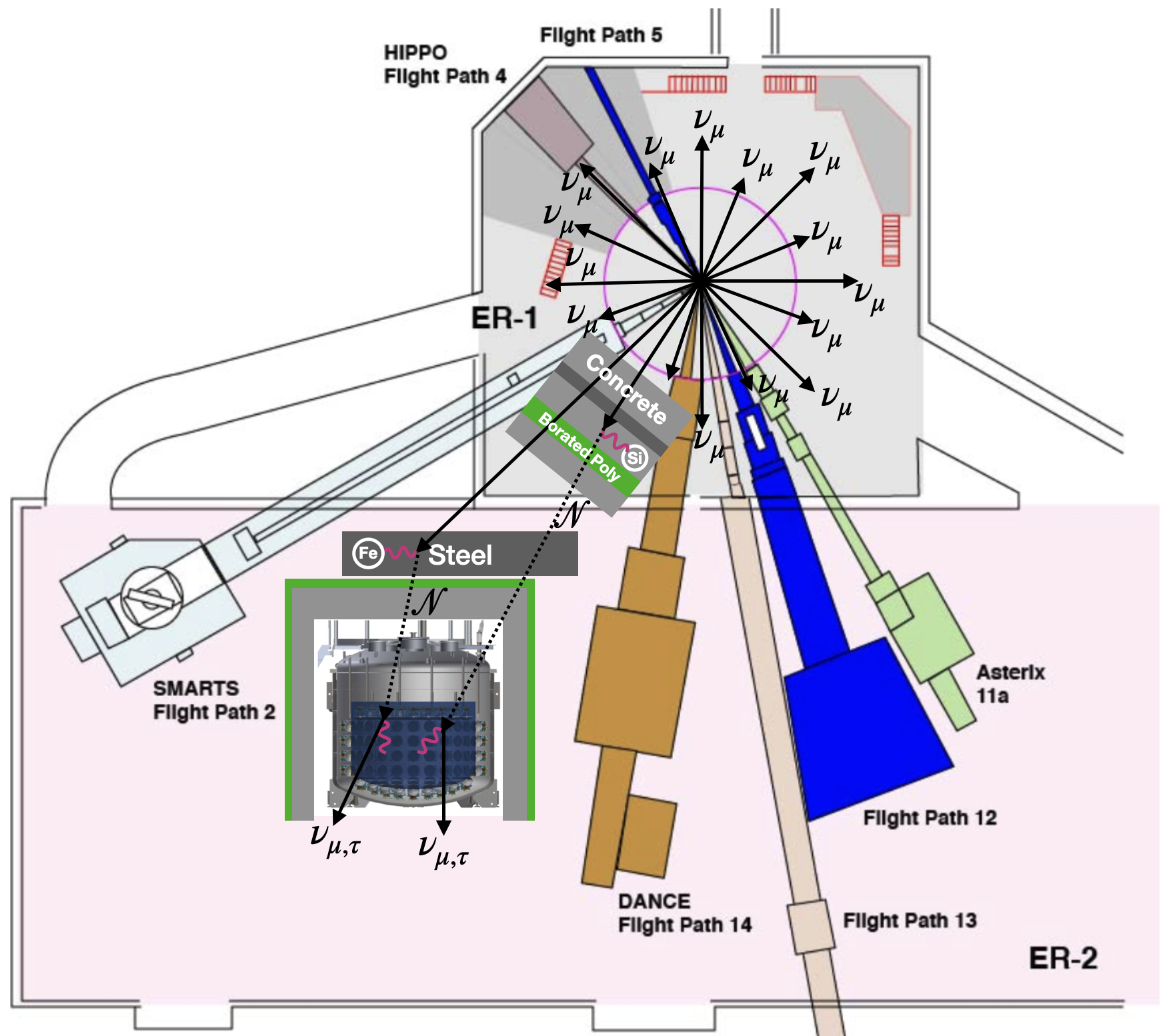
Figure 7.16: Schematic depiction of prompt $\nu_{\mu}$ from $\pi^{+}$ decay in the Lujan target upscattering to neutrissimos within shielding along the path to CCM200 and decaying to photons in the detector. The pink circle represents the TMRS shown in figure 7.1.

The beam-dump source at Lujan is an ideal location to look for neutrissimos. The prompt $\nu_{\mu}$ flux at CCM’s location is $4.74\times 10^{5}~{}\nu/{\rm cm}^{2}/s$ [30], corresponding to roughly $3.76\times 10^{-2}~{}\nu/{\rm POT}$. These neutrinos can undergo Primakoff upscattering in the shielding around the target and along the flight path to the detector, creating a flux of neutrissimos. These neutrissimos can decay within the CCM detector to photons with $E_{\gamma}\sim 15~{}{\rm MeV}$, which is relatively high energy compared to the background energy distribution [271]. A schematic depiction of this process is shown in figure 7.16. In this section, we define the neutrissimo signal as a single high energy photon in the detector. We do not evaluate our sensitivity to the coincidence channel discussed in Ref. [236], as the energy threshold of CCM does not yet enable CE$\nu$NS detection. Additionally, though we only consider neutrissimo production via Primakoff upscattering, neutrissimos can also be produced by the $\pi^{0}\to\gamma(\gamma^{*}\to\nu\mathcal{N})$ and $\gamma\nu\to\mathcal{N}$ channels within the target. Careful consideration of these additional detection and production channels may boost CCM’s sensitivity to neutrissimos, especially once the energy threshold is sufficiently lowered to enable a CE$\nu$NS search.

As we rely on monoenergetic $\nu_{\mu}$ with $E_{\nu}\sim 30~{}{\rm MeV}$ to undergo upscattering, we are sensitive to neutrissimos with $m_{\mathcal{N}}\lesssim 30~{}{\rm MeV}$. We simulate neutrissimo upscattering and decay using the updated LeptonInjector [262] simulation framework. The public version of LeptonInjector includes a geometry file with a realistic description of the CCM200 detector and the surrounding Lujan facility, including the shielding shown in figure 7.16 and the TMRS shown in figure 7.1 as well as the concrete floor. Monoenergetic muon neutrinos are injected as an isotropic point source originating from the center of the lower tungsten target. We sample an upscattering location along the flight path to CCM, considering only a cone surrounding the CCM detector to improve the simulation efficiency. We then sample a neutrissimo decay location. If the neutrissimo path crosses the CCM200 fiducial volume, its decay is required to occur within this volume to further improve the simulation efficiency. We save the four-momentum and physical event weight (in units of POT^-1) for the final state photon. By scaling to the expected CCM200 exposure of $2.25\times 10^{22}$ POT, we can estimate the single photon event rate from neutrissimo decay in the total three-year CCM200 dataset. This LeptonInjector-based CCM200 neutrissimo simulation was presented to the public during the 2023 CCM Workshop [261].

To assess sensitivity, we consider the background estimation from the ALP search [271], as this analysis used a similar electromagnetic final state signal definition. A sizable reduction in the background rate is expected for CCM200 compared to CCM120; the improved shielding already gives about an order-of-magnitude improvement [275], and the Cherenkov reconstruction simulation study described in section 7.2.1 suggests an additional two orders of magnitude in background reduction for a 5 MeV electron. In reporting results, we show a projected sensitivity range based on a background reduction within $[10^{-4},10^{-2}]$. The exact background reduction achieved by CCM200 will depend on the performance of the final Cherenkov reconstruction and argon filtration system as well as any improvements to the existing analysis cuts described in Ref. [271]. We assume a neutrissimo detection efficiency of 1.0, which is consistent with the expected ALP detection efficiency after CCM200 upgrades [275]. The photon energies are smeared according to an energy resolution of 15%, such that the prediction in each reconstructed energy bin $\mu_{i}$ is given by

$$\mu_{i}=\sum_{j=0}^{N_{\rm sim}}\int_{E_{i}^{\rm low}}^{E_{i}^{\rm high}}\frac{w_{j}}{\sqrt{2\pi(0.15E_{j})^{2}}}e^{\frac{-(E-E_{j})^{2}}{2(0.15E_{j})^{2}}}dE,$$ (7.9)

where $N_{\rm sim}$ is the number of simulated photons, $E_{i}^{\rm low}$ and $E_{i}^{\rm high}$ are the boundaries of reconstructed energy bin $i$, and $w_{j}$ and $E_{j}$ are the weight and energy of the $j^{\rm th}$ simulated photon from LeptonInjector. This energy resolution is relatively consistent with the CCM120 energy resolution at $E_{\gamma}\sim 20~{}{\rm MeV}$ [275] and a safe assumption once the updated Cherenkov reconstruction is in place.

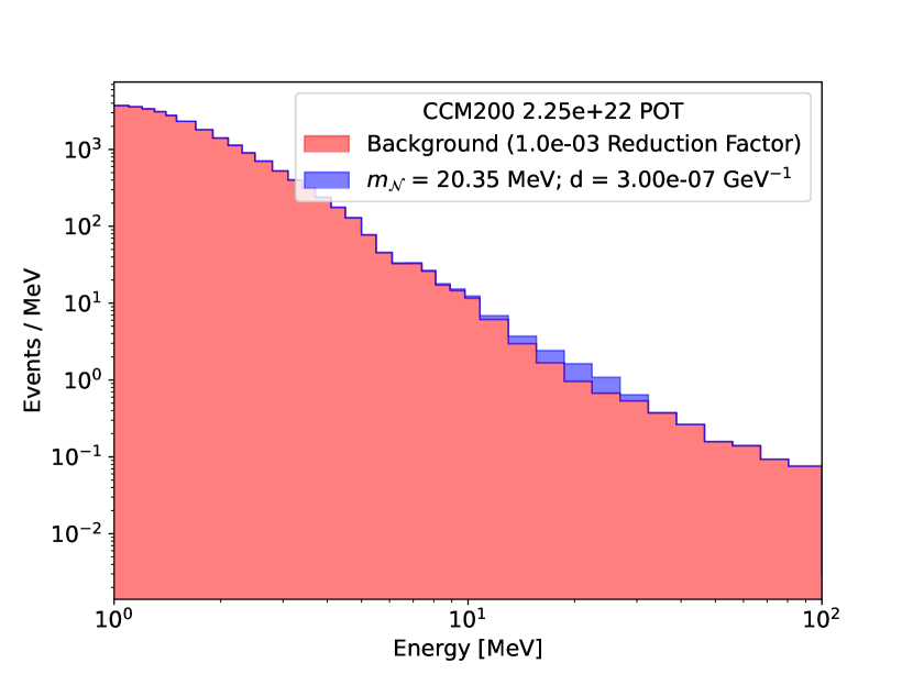
(a)

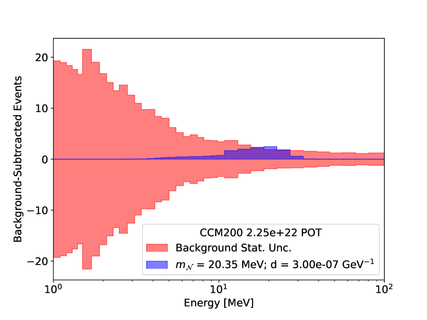
Figure 7.17: Figure 7.17(a) shows the distribution of background and signal prediction in CCM200 for $m_{\mathcal{N}}=20.35~{}{\rm MeV}$ and $d_{\mu{\mathcal{N}}}=3\times 10^{-7}~{}{\rm GeV}^{-1}$, considering a background reduction factor of $10^{-3}$ compared to CCM120. Figure 7.17 shows the background-subtracted plot, with a red band indicating the expected statistical uncertainty on the background.

We have run a series of simulations for neutrissimos with masses $m_{\mathcal{N}}[{\rm MeV}]\in[1,28]$ and dipole couplings $d_{\mu\mathcal{N}}[{\rm GeV}^{-1}]\in[10^{-7},10^{-5}]$. Figure 7.17 shows the expected energy distribution of neutrissimo decay signal events and background events in CCM200 for $m_{\mathcal{N}}=20.35~{}{\rm MeV}$ and $d_{\mu{\mathcal{N}}}=3\times 10^{-7}~{}{\rm GeV}^{-1}$, considering a background reduction factor of $10^{-3}$. The single photons from neutrissimo decay peak at $E_{\gamma}\sim 20~{}{\rm MeV}$, as expected. We calculate the CCM200 sensitivity across parameter space using the $\chi^{2}$ test statistic,

$$\chi^{2}(m_{\mathcal{N}},d_{\mu\mathcal{N}})=\sum_{i}\bigg{(}\frac{\mu_{i}(m_{\mathcal{N}},d_{\mu\mathcal{N}})}{\sigma_{i}}\bigg{)}^{2},$$ (7.10)

where $\mu_{i}(m_{\mathcal{N}},d_{\mu\mathcal{N}})$ is the neutrissimo prediction in the $i^{\rm th}$ reconstructed energy in and $\sigma_{i}$ is the statistical $\oplus$ systematic error on the background, appropriately scaled from Table 6.1 of Ref. [275]. We assume a $\chi^{2}$ distribution with two degrees of freedom to draw projected sensitivities at the 95% confidence level (corresponding to a critical value of $\chi^{2}=6.18$). Figure 7.18(a) shows the preliminary projected CCM200 sensitivity to neutrissimo parameter space over the full three-year run. If we achieve a background reduction factor closer to $10^{-4}$, CCM200 should be able to set world-leading constraints on the $d_{\mu\mathcal{N}}$ dipole coupling for $m_{\mathcal{N}}\sim 20~{}{\rm MeV}$. As discussed in section 6.4, flavor-conserving UV completions of the dipole operator predict larger branching ratios for the decay $\mathcal{N}\to\nu_{\tau}\gamma$. As the neutrissimo single photon rate in CCM200 is primarily limited by the neutrissimo decay probability within the detector, CCM200 will be more sensitive to a scenario with such flavor-dependent dipole couplings. In figure 7.18(b) we show a preliminary estimate of CCM200’s sensitivity to the $d_{\tau{\mathcal{N}}}=d_{\mu{\mathcal{N}}}m_{\tau}/m_{\mu}$ discussed in section 6.4. The full CCM200 dataset will exclude a large region of the available parameter space in this flavor-dependent dipole model.

A few points are worth noting regarding these preliminary sensitivities. First, while the LeptonInjector simulation of CCM200 provides a relatively precise initial estimate of the neutrissimo decay rate in the detector, the geometric description of the Lujan facility will need to be verified before these sensitivities are ready for publication. This is especially true considering the strong dependence of the neutrissimo event rate on the exact shielding configuration between the tungsten target and the detector. That being said, any updates to the LeptonInjector CCM200 geometry made during this verification process are likely to be small and thus will not drastically shift the sensitivities in figure 7.18. The sensitivity might also improve after considering the additional neutrissimo production and detection mechanisms discussed earlier: $\pi^{0}\to\gamma\nu\mathcal{N}$ and $\gamma\nu\to\mathcal{N}$ within the target, and nuclear recoil from Primakoff upscattering within the detector. These are all possible to simulate within LeptonInjector. The $\pi^{0}$ and $\gamma$ flux were calculated for the ALP analysis [271], and nuclear recoil kinematics are already simulated within LeptonInjector. These channels will be carefully evaluated as the CCM200 neutrissimo analysis is prepared for publication. Further improvements to CCM200’s sensitivity can be made for modified shielding configurations that introduce some amount of high-$Z$ material, such as lead ($Z=82$), in order to benefit from the $Z^{2}$ coherent enhancement of the Primakoff upscattering cross section [31]. Potential improved shielding configurations can and will be studied within LeptonInjector.

One must also consider the timing distribution of the photons from neutrissimo decay within the detector. CCM relies on strict timing cuts to remove neutron backgrounds; thus, it is important to ensure that the added travel time of non-relativistic neutrissimos does not push these photons outside of the CCM ROI. This is easily studied within LeptonInjector, as the entire path of the neutrino and neutrissimo is computed for each simulated event. Figure 7.19 shows the added time delay from the neutrissimo flight path for $m_{\mathcal{N}}=20.35~{}{\rm MeV}$ (note that the time delay does not depend on the dipole coupling to first order). This is the most important neutrissimo mass to check, as it corresponds to the strongest projected constraints in figure 7.18. Two distinct populations can be seen at 5 ns and 26 ns, corresponding to upscattering in the shielding surrounding CCM and the TMRS, respectively. This suggests characteristic time delays $\Delta t\lesssim 30~{}{\rm ns}$, which is comfortably within the 150 ns ROI of the ALP analysis [271]. Thus, the CCM timing cuts should not be an issue for the neutrissimo model.

The analysis presented here can in principle be used to set constraints using CCM120 data. However, the signal efficiency of neutrissimo events must be more carefully evaluated for this dataset. The CCM120 ALP analysis used a variety of cuts on the event length, reconstructed radius, and PMT charge uniformity to remove backgrounds. While the improvements made for CCM200 are likely to push the ALP (and thus neutrissimo) selection efficiency to greater than $0.95$, the CCM120 ALP selection efficiency fell roughly within $[0.2,0.4]$ depending on the ALP energy [271]. Further, the CCM120 analysis used only the first 38 ns of each event to calculate the reconstructed energy [271], which will have a nontrivial impact on the assumed 15% symmetric energy resolution. Finally, the shielding configuration was updated between CCM120 and CCM200, and the CCM120 version is not currently modeled in LeptonInjector. We will need to study the impact of all of these effects on single photon events before calculating CCM120 limits on the neutrissimo model.

The analysis presented in this section highlights the strong capability of CCM in constraining BSM physics. The high-intensity beam dump at the Lujan center can produce a significant number of potential BSM particles, while the extremely low duty factor helps isolate these particles from SM backgrounds. The large size, good energy resolution, and fast timing response of the CCM detector are well-suited for measuring any potential interactions of these BSM particles. The neutrissimo model discussed here is just one of many BSM scenarios on which CCM200 will place world-leading constraints [30, 271, 270, 145]. Additionally, the neutrissimo model specifically emphasizes the significant impact that Chernekov light reconstruction will have on CCM200 sensitivity to BSM interactions with electromagnetic final states (which also occur in the ALP model).

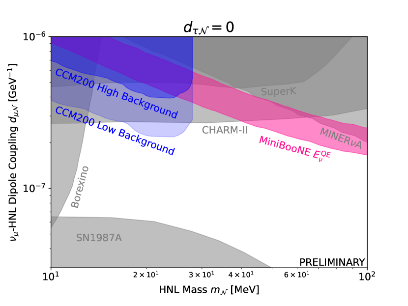
(a)

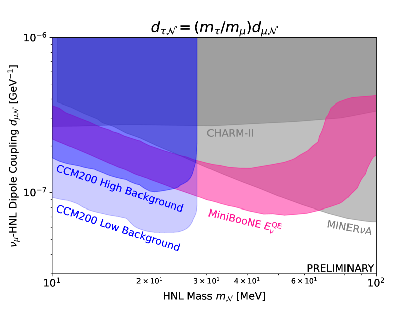
(b)

Figure 7.18: Figure 7.18(a) shows the expected sensitivity of CCM200 to the neutrissimo model, where the blue band corresponds to a background reduction factor between $10^{-4}$ (“CCM200 Low Background”) and $10^{-2}$ (“CCM200 High Background”). The MiniBooNE $E_{\nu}^{\rm QE}$ allowed region (pink) and existing constraints (grey) come from Ref [31]. Figure 7.18(b) shows the same plot, but considering $\mathcal{N}\to\nu_{\tau}\gamma$ decays with $d_{\tau{\mathcal{N}}}=d_{\mu{\mathcal{N}}}m_{\tau}/m_{\mu}$.

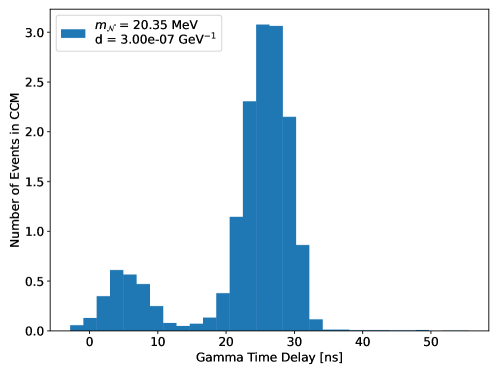
Figure 7.19: The time delay of neutrissimo single photon decays with the CCM detector for the indicated mass and coupling, as calculated using LeptonInjector.

Chapter 8 Conclusions and Future Prospects

This thesis presents an array of experimental and phenomenological investigations into the nature of the MiniBooNE low energy excess (LEE). The MiniBooNE LEE, described in detail in chapter 2, refers to the $4.8\sigma$ excess of electron-like neutrino interactions observed by the MiniBooNE detector along the Booster Neutrino Beamline (BNB) [10]. This is one of the most significant and longest-standing anomalies with respect to the Standard Model (SM) of particle physics. The excess has remained consistent over the full 17-year dataset, corresponding to $18.75\times 10^{20}$ ($11.27\times 10^{20}$) protons-on-target (POT) in neutrino (antineutrino) mode. Due to the nature of a Cherenkov detector, MiniBooNE could not distinguish between electrons, photons, or collimated $e^{+}e^{-}$ pairs–thus, any of these can contribute to the MiniBooNE LEE. Though SM explanations of the excess have been investigated thoroughly, both internally within MiniBooNE [10] and by the external community [81, 80], no promising SM candidates have emerged. Thus, the MiniBooNE LEE may be an indication of beyond-the-SM (BSM) physics. The most common BSM interpretation of the MiniBooNE anomaly is the $3+1$ model, which predicts $\nu_{\mu}\to\nu_{e}$ and $\overline{\nu}_{\mu}\to\overline{\nu}_{e}$ oscillations at short baseline through an eV-scale sterile neutrino. This is an attractive solution as it would also explain the anomalous excess of $\overline{\nu}_{e}$ interactions observed by the LSND experiment, which was the original physics motivation behind the MiniBooNE experiment.

The MicroBooNE experiment was conceived to follow up on the MiniBooNE LEE. MicroBooNE uses a liquid argon time projection chamber (LArTPC) detector [16], described in detail in chapter 3, to observe the interactions of neutrinos along the BNB. The detailed images of neutrino interactions produced by the LArTPC enable the separation of events with electrons and photons in the final state, allowing a suite of analyses looking for different explanations of the MiniBooNE excess. My research within MicroBooNE focused on the “two-body CCQE analysis”: a search for $\nu_{e}$ charged-current quasi-elastic (CCQE) interactions consistent with two-body scattering kinematics [148]. This analysis is described in detail in chapter 4. It uses a variety of techniques [24, 172], including several deep-learning-based methods [21, 22], to reconstruct and isolate signal events from backgrounds. The electromagnetic shower reconstruction, which drives the reconstruction of the original neutrino energy, is validated using two data-driven standard candles: the $\pi^{0}$ invariant mass peak and the Michel electron energy spectrum cutoff [172]. This study is presented in section 4.4.3. The most powerful technique used in the signal selection leverages an ensemble of boosted decision trees (BDTs) trained on a collection of variables describing the topology and kinematics of candidate $\nu_{e}$ CCQE interactions. This BDT ensemble is specifically tailored to select events consistent with a clean two-body interaction, which helps reduce the impact of complicated nuclear effects on our signal prediction.

The two-body CCQE analysis observed 25 events passing all signal selection requirements in the first $6.67\times 10^{20}$ POT of BNB data [148]. The statistical results from this dataset are presented in chapter 5. The two-body CCQE analysis does not observe significant excess of $\nu_{e}$ CCQE events at the lowest energies consistent with the MiniBooNE LEE. Using a two-hypothesis test and the CL_s test statistic, we are able to rule out the median expectation from the MiniBooNE excess at the $2.4\sigma$ confidence level. A signal strength scaling test performed using the Feldman-Cousins procedure sets an upper bound of $0.38$ on the $\nu_{e}$ fractional contribution to the MiniBooNE LEE at the $2\sigma$ confidence level. The results obtained by our analysis are consistent with the other two MicroBooNE $\nu_{e}$ analysis–no analysis observes a significant low-energy excess of charged-current $\nu_{e}$ interactions like that predicted by the MiniBooNE LEE [116].

Two external follow-studies regarding the MicroBooNE results are presented. The first of these is a combined fit of MicroBooNE and MiniBooNE data to the $3+1$ model [102], presented in section 5.3.1. This study shows that despite the strong constraints from MicroBooNE on $\nu_{e}$ interpretations of the MiniBooNE LEE, closed contours in $3+1$ parameter space still exist at the $3\sigma$ confidence level in the combined MiniBooNE-MicroBooNE fit. Thus, the MicroBooNE results do not definitively rule out the $3+1$ interpretation of the MiniBooNE excess. The second study, presented in section 5.3.2, looked into the implications of a $\overline{\nu}_{e}$ explanation of the MiniBooNE excess [201]. Due to the isoscalar and non-isoscalar nature of the carbon and argon nucleus, respectively, the $\overline{\nu}_{e}$ cross section tends to be much more suppressed at low energy in argon compared to carbon, while the same is not true for $\nu_{e}$ interactions. Thus, MicroBooNE will be less sensitive to the MiniBooNE LEE if it comes from $\overline{\nu}_{e}$ interactions. Ref. [201] shows that the MicroBooNE data are consistent at the $2\sigma$ confidence level with a scenario in which the MiniBooNE excess is comprised entirely of $\overline{\nu}_{e}$ events.

In chapter 6 we discuss a mixed model comprising an eV-scale sterile neutrino and an MeV-scale heavy neutral lepton with a dipole coupling to active neutrinos, referred to as a neutrissimo $\mathcal{N}$ [27, 31]. It is shown that this model can significantly relax the internal tension in global $3+1$ by explaining the bulk of the MiniBooNE excess through neutrissimo decays to single photons. As discussed in section 6.3, the neutrissimo with $m_{\mathcal{N}}\sim 500~{}{\rm MeV}$ can simultaneously provide a good explanation to the energy and angular distributions, which is not possible within the $3+1$ model alone. In Ref. [31], we have calculated world-leading constraints on the neutrissimo model using the high $dE/dX$ sideband of the MINER$\nu$A elastic scattering analyses. This study is presented in section 6.4. While the MINER$\nu$A constraints are indeed very strong in the $m_{\mathcal{N}}=\mathcal{O}(100~{}{\rm MeV})$ region, they do not rule out the MiniBooNE-preferred region in neutrissimo parameter space at the 95% confidence level. This is because the kinematic cuts in the MINER$\nu$A analysis remove a majority of neutrissimo events for $m_{\mathcal{N}}\sim 500~{}{\rm MeV}$. A dedicated MINER$\nu$A analysis would likely be able to make a definitive statement on the neutrissimo explanation of the MiniBooNE LEE.

Finally, we close with the Coherent CAPTAIN-Mills (CCM) experiment in chapter 7. CCM uses a liquid argon detector at the Lujan proton beam dump facility of the Los Alamos Neutron Science Center (LANSCE) to look for the interactions of potential beyond-the-Standard-Model (BSM) particles. The CCM detector uses an array of photo-multiplier tubes (PMTs) to observe the scintillation light produced in these interactions. CCM leverages the low duty factor of the Lujan beam dump to make strict timing cuts on signals coming from the beam, isolating prompt signal events corresponding to BSM particles from slower beam-related neutron backgrounds. This strategy has allowed CCM to place strong limits on a wide variety of BSM scenarios, including light vector-portal dark matter [30], leptophobic dark matter [270], and axion-like-particles [271], using only data from a six-week 120-PMT engineering run. The full 200-PMT detector, “CCM200”, started taking data in Summer 2022 for its nominal three-year run at the Lujan facility. CCM200 will make a number of improvements upon the 120-PMT engineering run, including upgraded shielding and the deployment of an argon filtration system, which will help set world-leading limits on these models.

One of the most promising improvements is the development of a Cherenkov light reconstruction algorithm, which can help separate BSM events with electromagnetic final states from SM backgrounds. Section 7.2.1 presents a simulation-based study that indicates the feasibility of Cherenkov reconstruction in CCM thanks to the combination of PMTs coated and uncoated with wavelength-shifting tetraphenyl butadiene. The study suggests that uncoated PMTs will be especially sensitive to Cherenkov light in the visible regime for the first $\sim 10~{}{\rm ns}$ of a given electromagnetic event. Section 7.2.2 discusses some of the initial steps toward developing the Cherenkov reconstruction in data, including the deployment of a dedicated cosmic muon trigger and improvements to the CCM pulse finding algorithm. We discuss a potential use-case for the Cherenkov reconstruction in section 7.3, which presents a calculation of CCM200’s sensitivity to the neutrissimo model discussed above. Preliminary estimates suggest that CCM200 will be sensitive to new regions of neutrissimo parameter space for $m_{\mathcal{N}}\sim 20~{}{\rm MeV}$ over its full three-year dataset.

Neutrinos have never failed to surprise us. Since the first detection of neutrinos in 1956, experimental anomalies like the solar neutrino problem and the atmospheric neutrino anomaly have provided a guiding light toward a more complete understanding of the “little neutral one”. The experimentally-established fact that neutrinos have nonzero mass is not predicted by the Standard Model, and the comparatively tiny neutrino mass with respect to other particles is a strong motivation for BSM physics. Anomalies in short baseline neutrino experiments could very well be hinting that the neutrino has secrets yet to reveal. This thesis takes a few concrete steps along the path lit by the MiniBooNE anomaly. Only time–and clever experimental analyses–will tell where this path leads.

Appendix A Publication: Convolutional neural networks for shower energy prediction in liquid argon time projection chambers

My first research project as a graduate student involved the development of a convolutional neural network for electromagnetic shower energy reconstruction in MicroBooNE. While the MicroBooNE network never saw the light of day, the network was adapted for use in general LArTPC experiments by an MIT undergraduate student, Kiara Carloni. Kiara led the study discussed in the JINST publication below [23]. I served mainly as a mentor for this project, as it was extended from my early MicroBooNE work.

See pages - of templates/Publications/Carloni_2022_J._Inst._17_P02022.pdf

Appendix B Signal Event Displays from the Two-Body CCQE Analysis

Figure 5.1 in chapter 5 shows the event display for one of the 25 $\nu_{e}$-candidate selected events in the $1e1p$ dataset. We provide the remaining 24 event displays in figure B.1 to figure B.24, in ascending order in energy. The top row of each display shows the pixel intensity image, while the bottom row shows the SparseSSNet pixel labels. From left to right, the columns correspond to the U,V, and Y plane images.

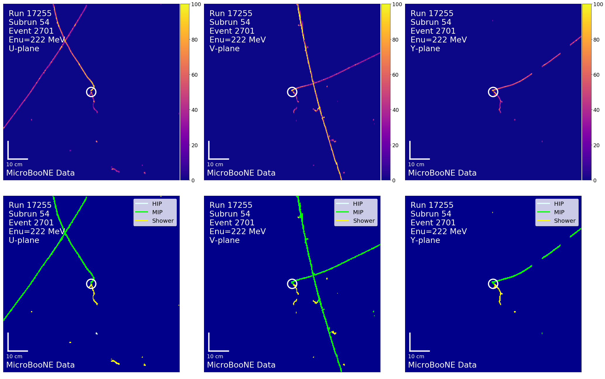
Figure B.1: Top: pixel intensity; Bottom: SparseSSNet labels; Left to right: U, V, Y, planes. The white circle indicates the reconstructed vertex.

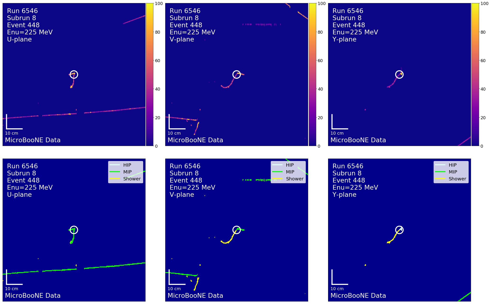
Figure B.2: Top: pixel intensity; Bottom: SparseSSNet labels; Left to right: U, V, Y, planes. The white circle indicates the reconstructed vertex.

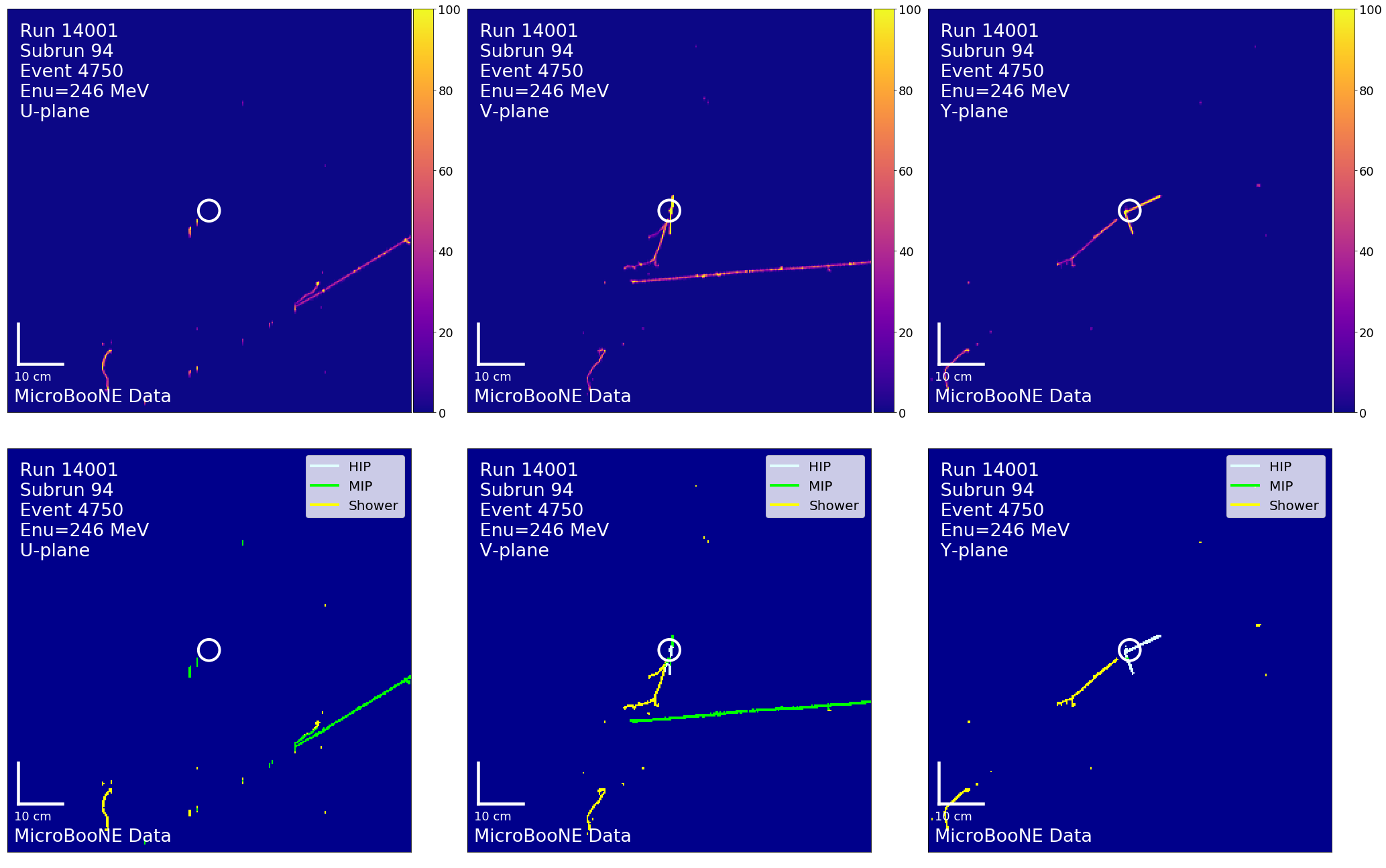
Figure B.3: Top: pixel intensity; Bottom: SparseSSNet labels; Left to right: U, V, Y, planes. The white circle indicates the reconstructed vertex.

Figure B.4: Top: pixel intensity; Bottom: SparseSSNet labels; Left to right: U, V, Y, planes. The white circle indicates the reconstructed vertex.

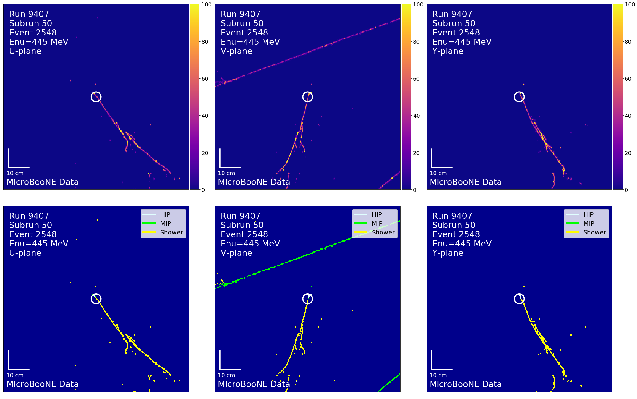
Figure B.5: Top: pixel intensity; Bottom: SparseSSNet labels; Left to right: U, V, Y, planes. The white circle indicates the reconstructed vertex.

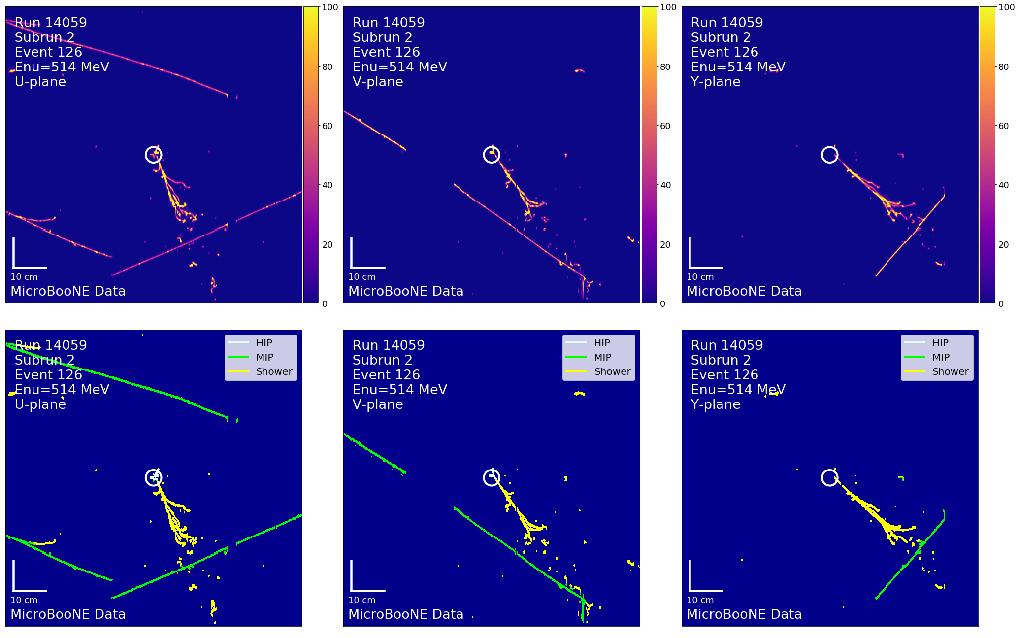
Figure B.6: Top: pixel intensity; Bottom: SparseSSNet labels; Left to right: U, V, Y, planes. The white circle indicates the reconstructed vertex.

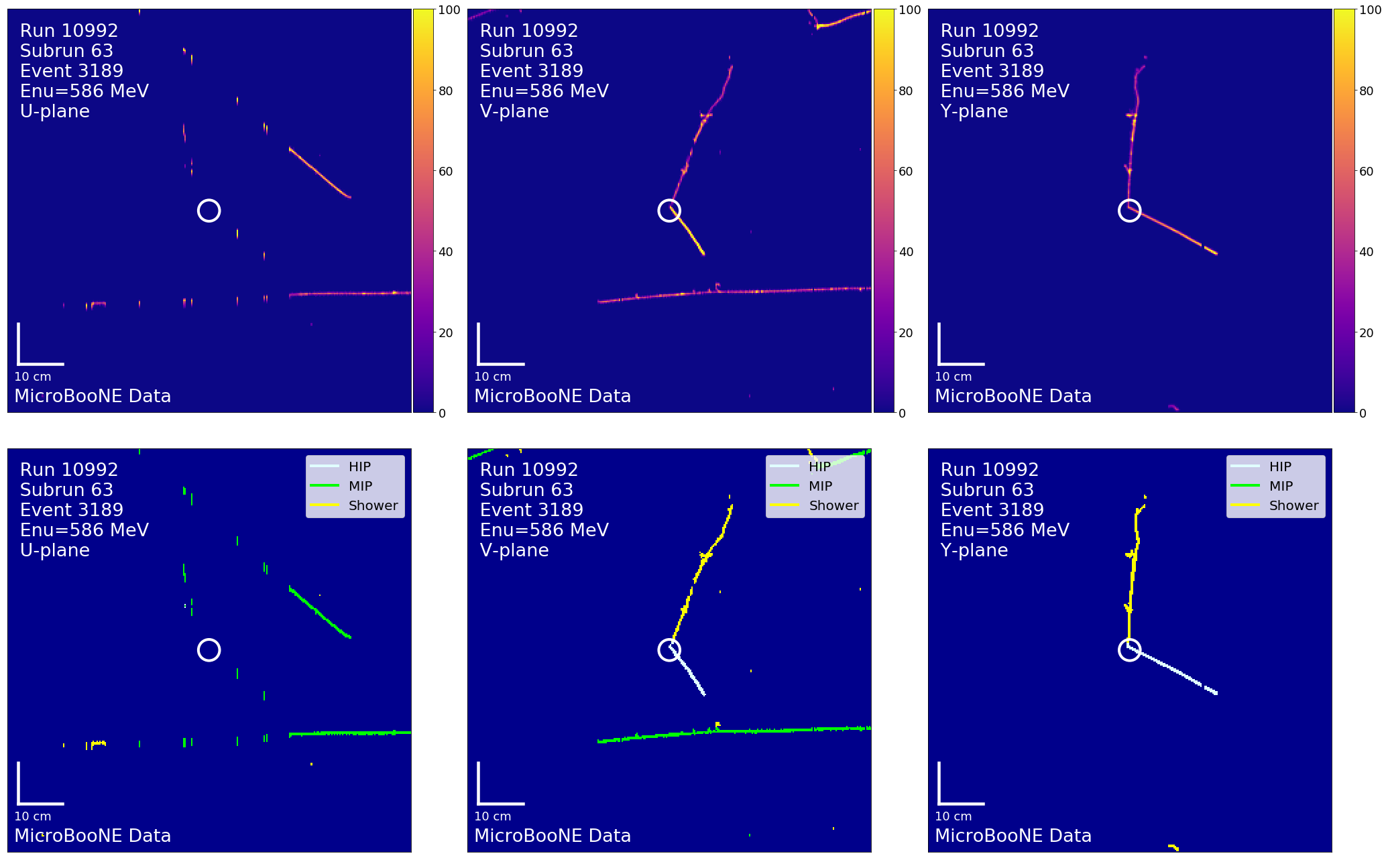
Figure B.7: Top: pixel intensity; Bottom: SparseSSNet labels; Left to right: U, V, Y, planes. The white circle indicates the reconstructed vertex.

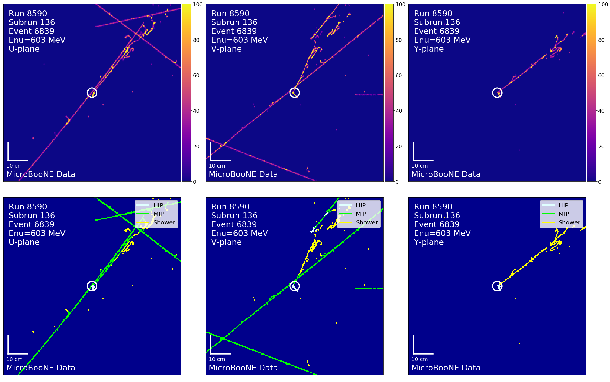
Figure B.8: Top: pixel intensity; Bottom: SparseSSNet labels; Left to right: U, V, Y, planes. The white circle indicates the reconstructed vertex.

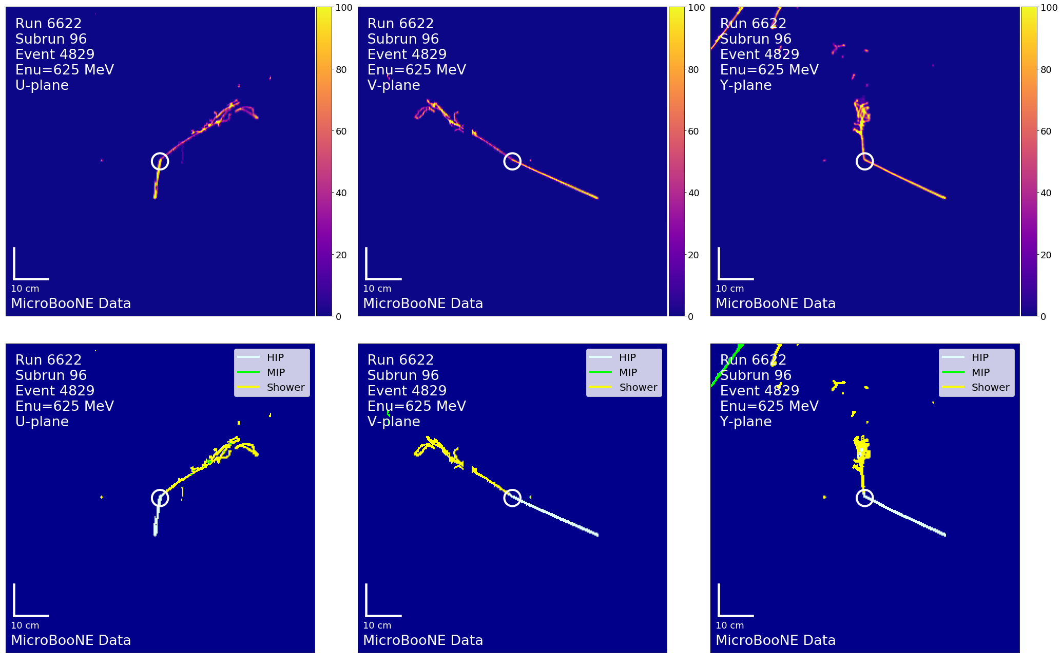
Figure B.9: Top: pixel intensity; Bottom: SparseSSNet labels; Left to right: U, V, Y, planes. The white circle indicates the reconstructed vertex.

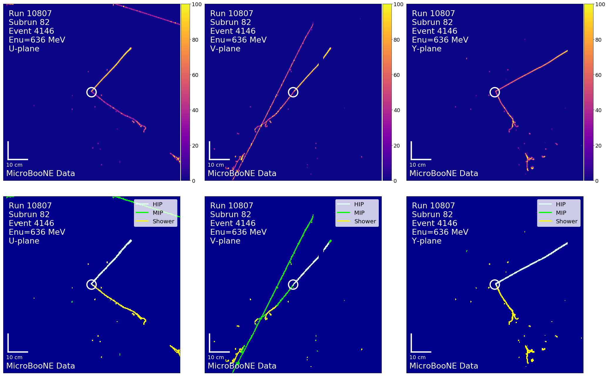
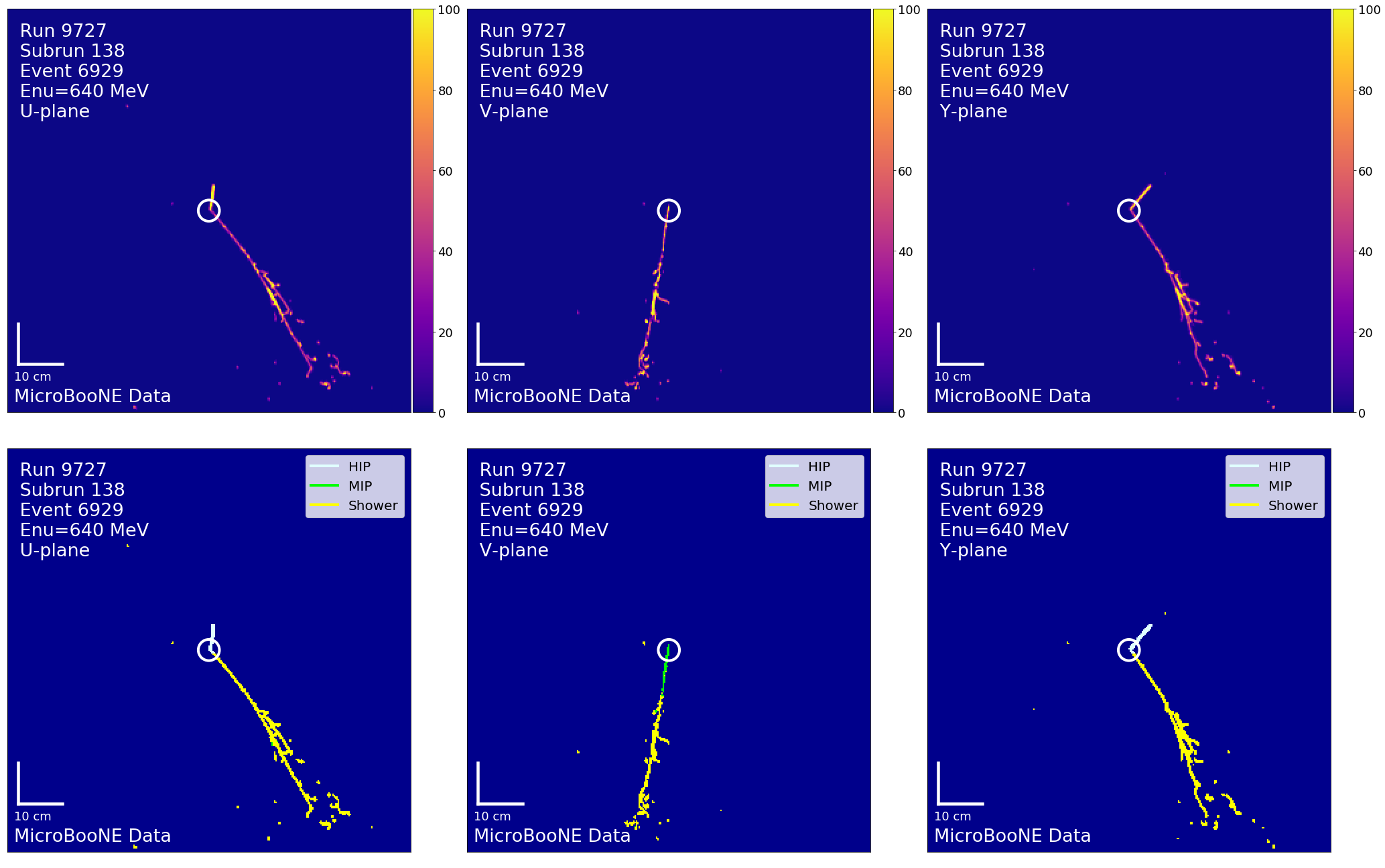
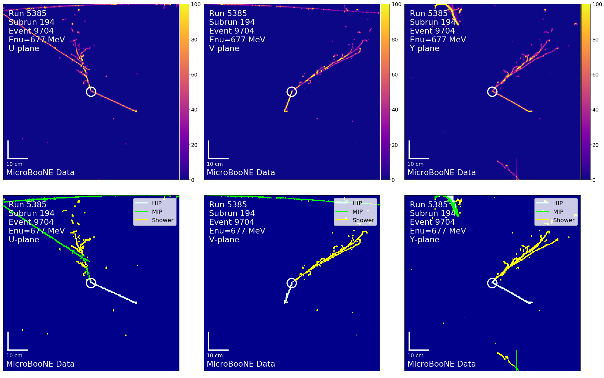
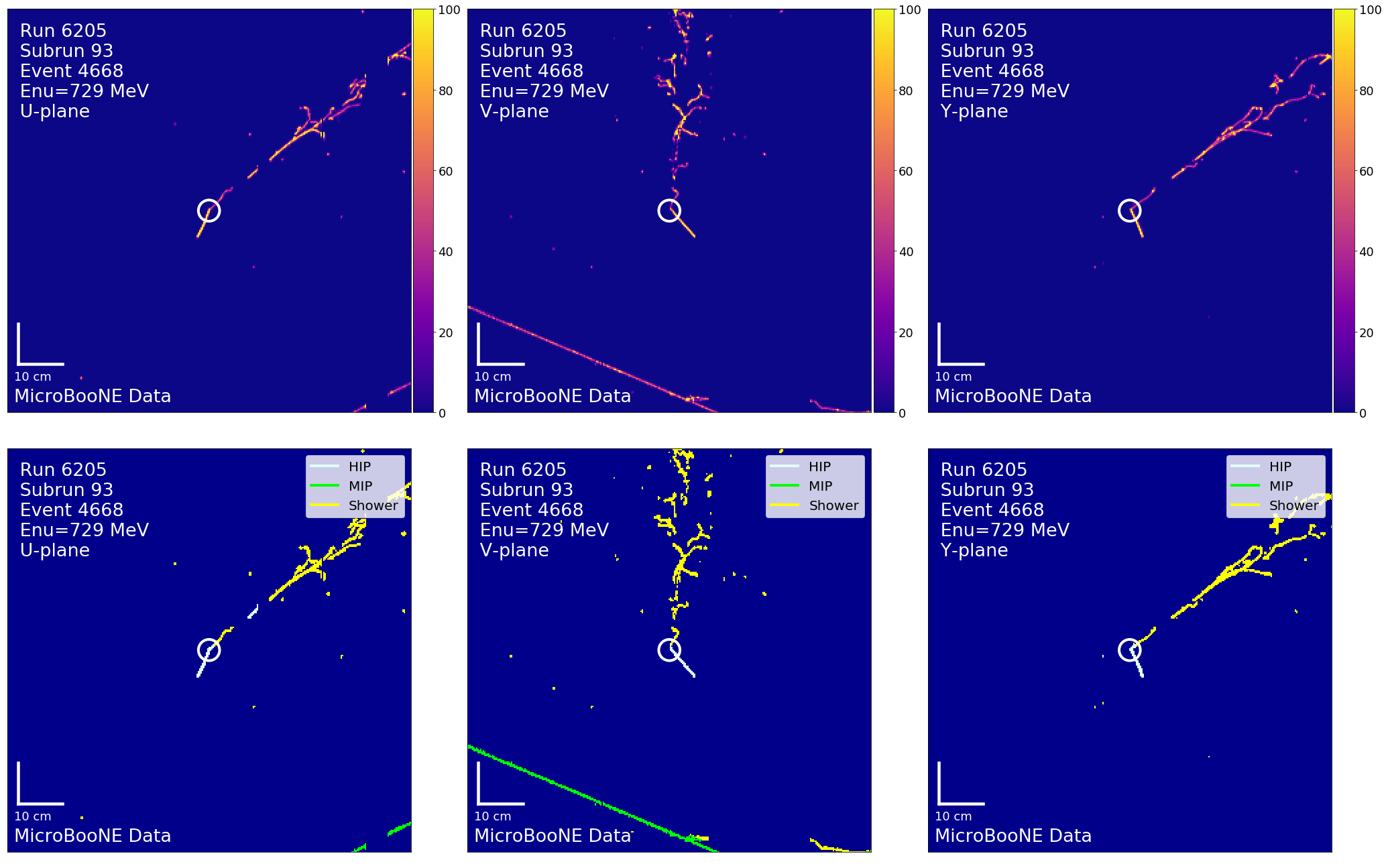
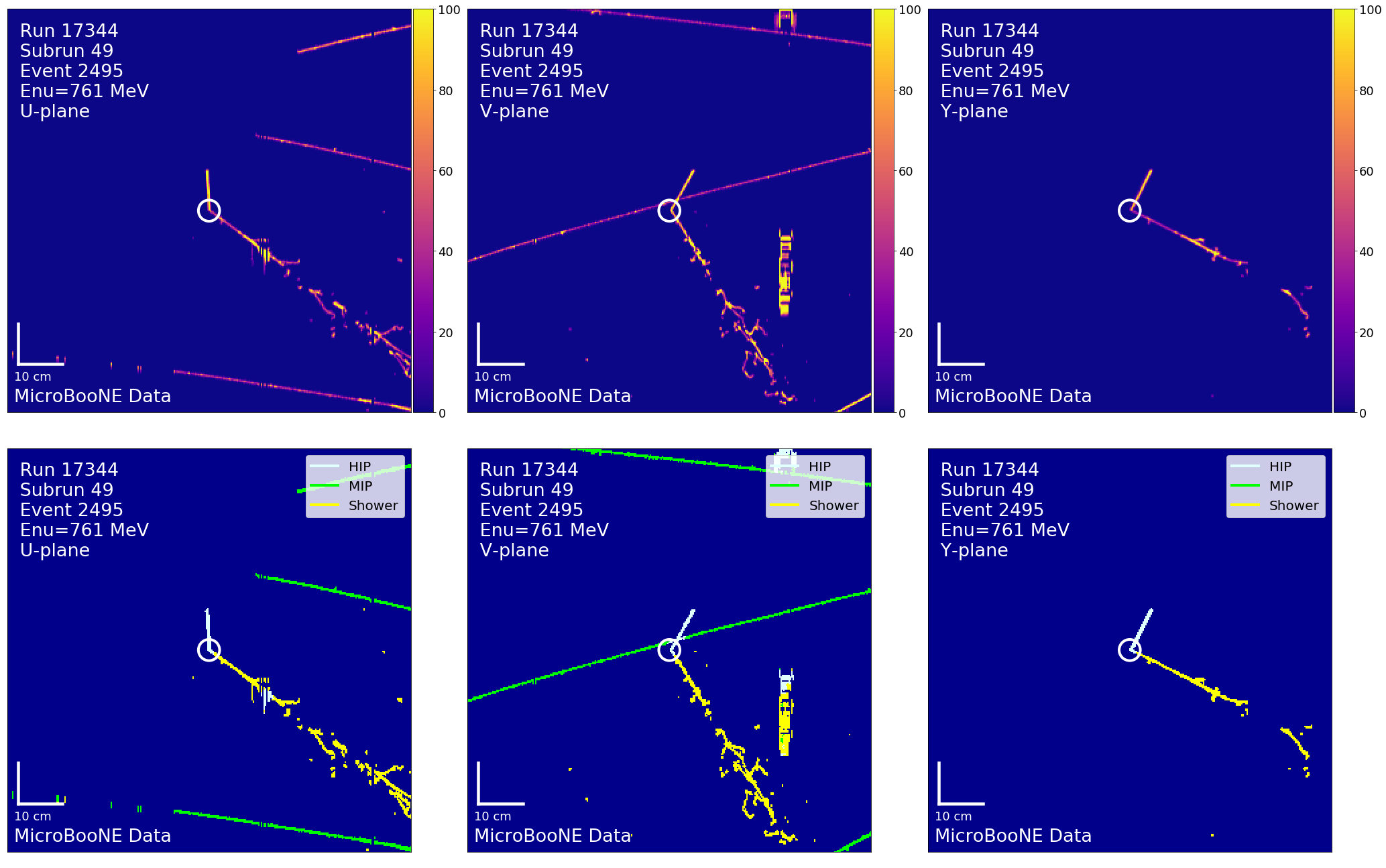
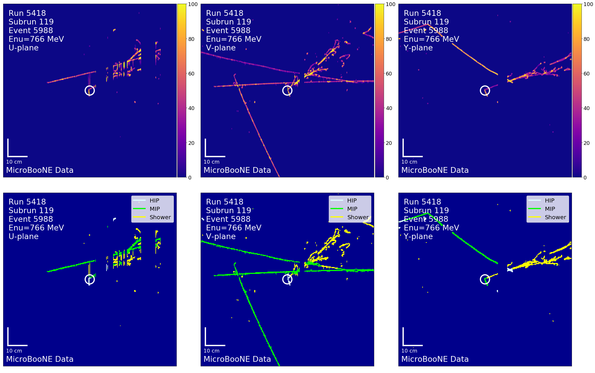
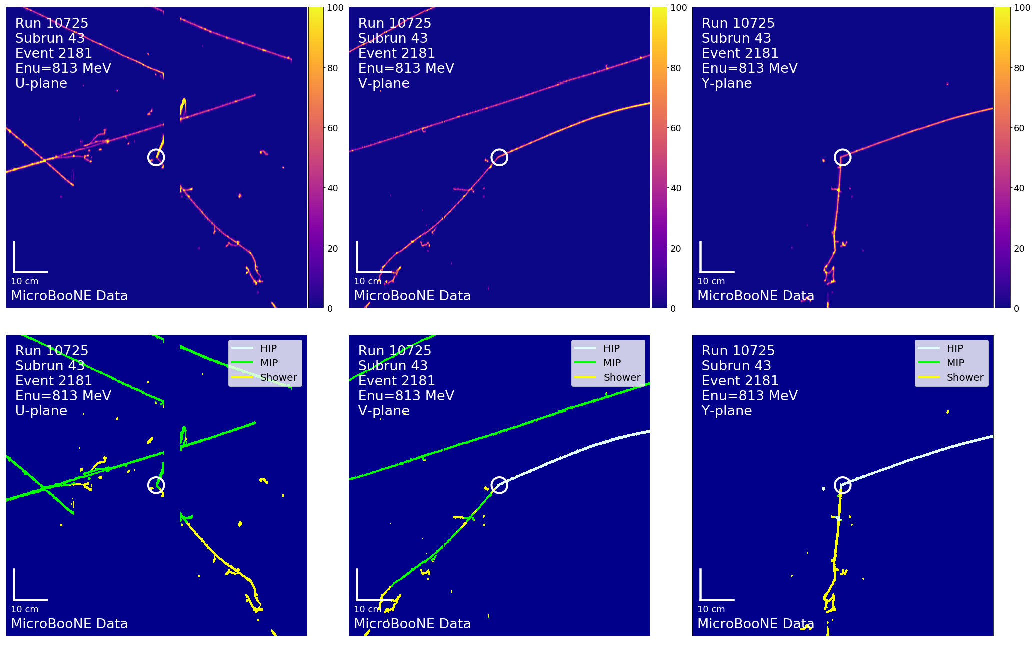
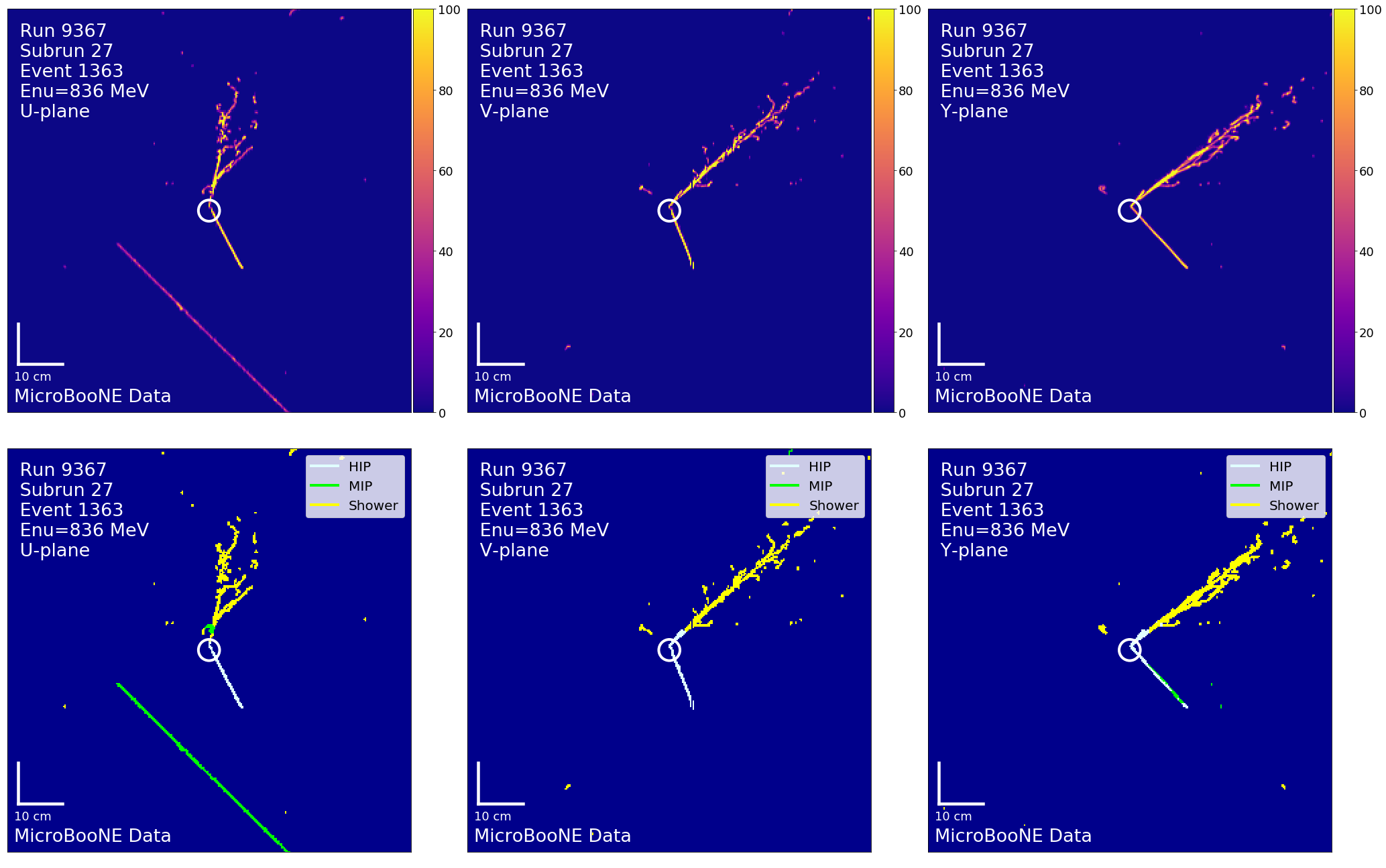
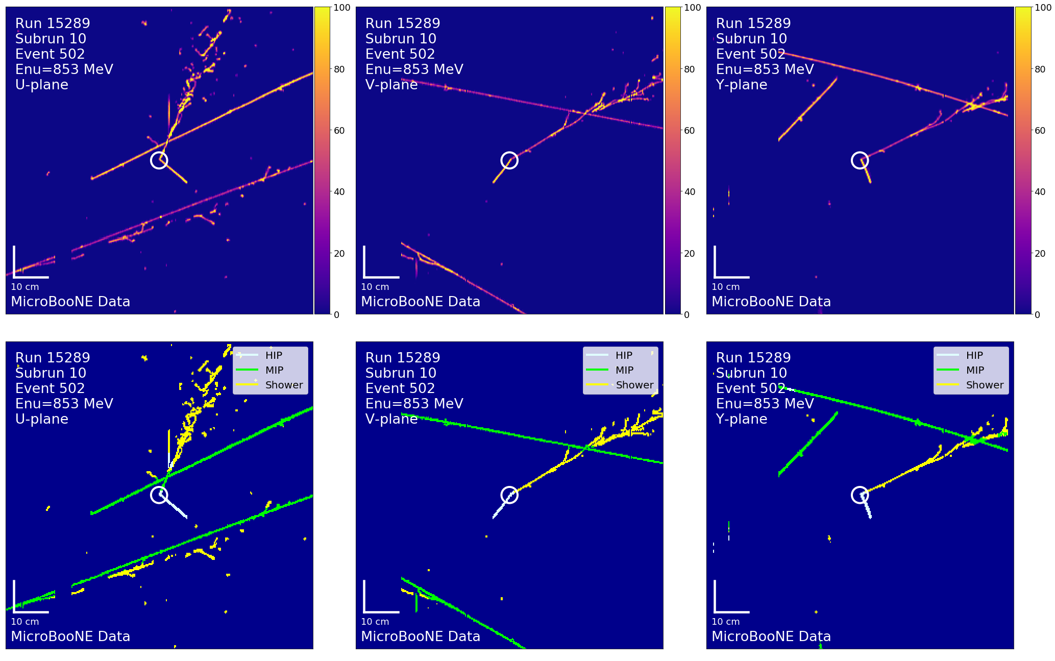
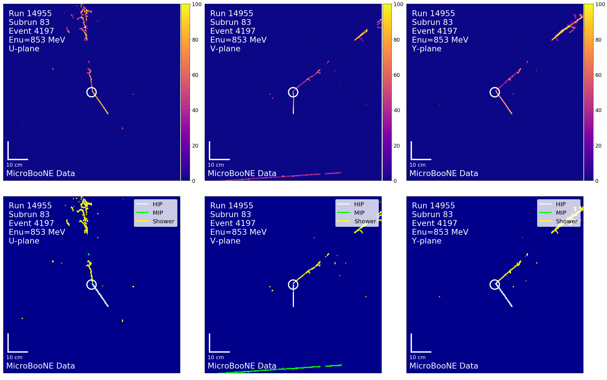
Figure B.10: Top: pixel intensity; Bottom: SparseSSNet labels; Left to right: U, V, Y, planes. The white circle indicates the reconstructed vertex.

Figure B.11: Top: pixel intensity; Bottom: SparseSSNet labels; Left to right: U, V, Y, planes. The white circle indicates the reconstructed vertex.

Figure B.12: Top: pixel intensity; Bottom: SparseSSNet labels; Left to right: U, V, Y, planes. The white circle indicates the reconstructed vertex.

Figure B.13: Top: pixel intensity; Bottom: SparseSSNet labels; Left to right: U, V, Y, planes. The white circle indicates the reconstructed vertex.

Figure B.14: Top: pixel intensity; Bottom: SparseSSNet labels; Left to right: U, V, Y, planes. The white circle indicates the reconstructed vertex.

Figure B.15: Top: pixel intensity; Bottom: SparseSSNet labels; Left to right: U, V, Y, planes. The white circle indicates the reconstructed vertex.

Figure B.16: Top: pixel intensity; Bottom: SparseSSNet labels; Left to right: U, V, Y, planes. The white circle indicates the reconstructed vertex.

Figure B.17: Top: pixel intensity; Bottom: SparseSSNet labels; Left to right: U, V, Y, planes. The white circle indicates the reconstructed vertex.

Figure B.18: Top: pixel intensity; Bottom: SparseSSNet labels; Left to right: U, V, Y, planes. The white circle indicates the reconstructed vertex.

Figure B.19: Top: pixel intensity; Bottom: SparseSSNet labels; Left to right: U, V, Y, planes. The white circle indicates the reconstructed vertex.

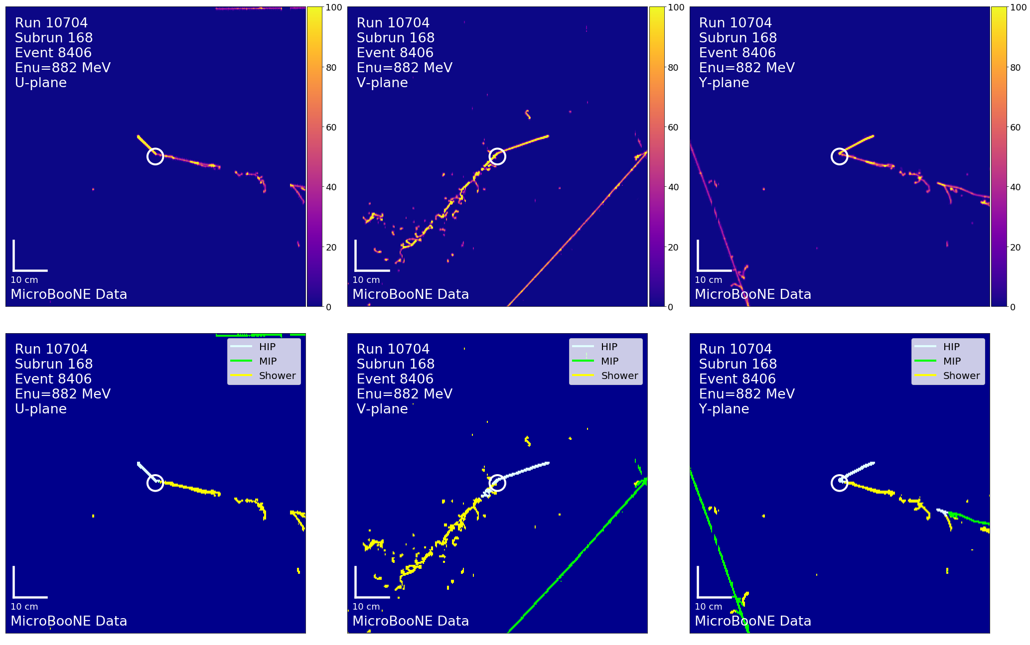
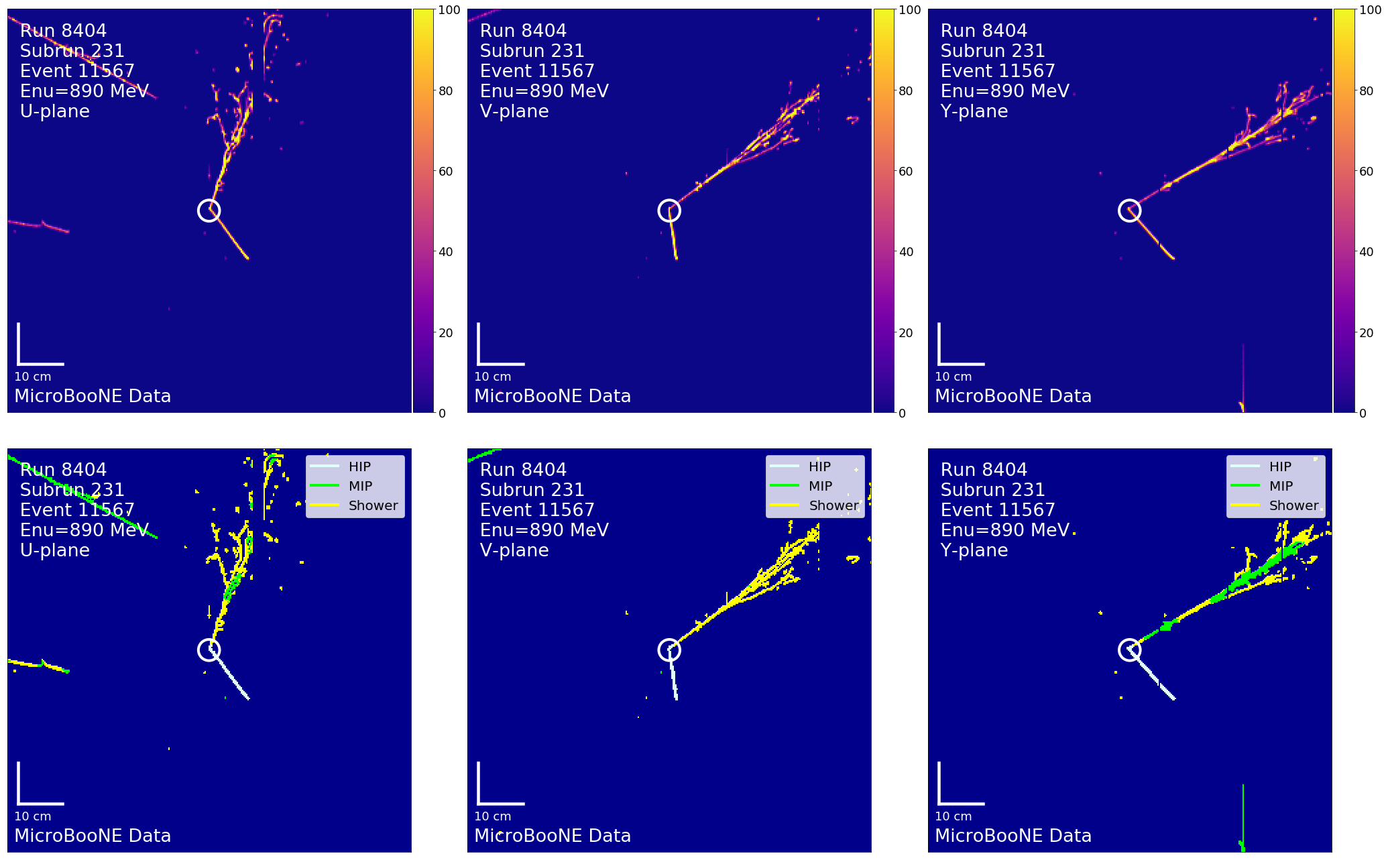
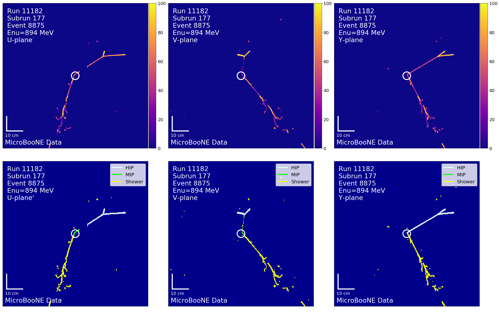
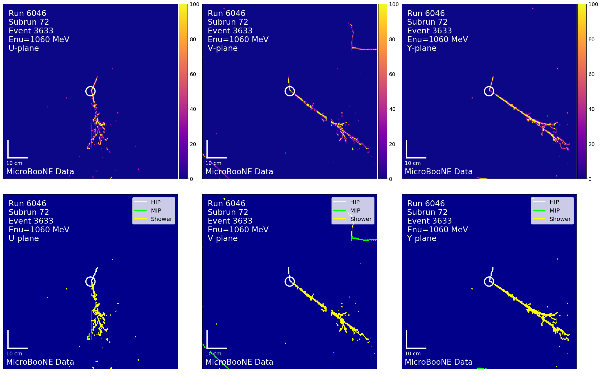
Figure B.20: Top: pixel intensity; Bottom: SparseSSNet labels; Left to right: U, V, Y, planes. The white circle indicates the reconstructed vertex.

Figure B.21: Top: pixel intensity; Bottom: SparseSSNet labels; Left to right: U, V, Y, planes. The white circle indicates the reconstructed vertex.

Figure B.22: Top: pixel intensity; Bottom: SparseSSNet labels; Left to right: U, V, Y, planes. The white circle indicates the reconstructed vertex.

Figure B.23: Top: pixel intensity; Bottom: SparseSSNet labels; Left to right: U, V, Y, planes. The white circle indicates the reconstructed vertex.

Figure B.24: Top: pixel intensity; Bottom: SparseSSNet labels; Left to right: U, V, Y, planes. The white circle indicates the reconstructed vertex.

References

- [1] John N. Bahcall. Solar models and solar neutrinos: Current status. Phys. Scripta T, 121:46–50, 2005.
- [2] Y. Fukuda et al. Evidence for oscillation of atmospheric neutrinos. Phys. Rev. Lett., 81:1562–1567, 1998.
- [3] Q. R. Ahmad et al. Direct evidence for neutrino flavor transformation from neutral current interactions in the Sudbury Neutrino Observatory. Phys. Rev. Lett., 89:011301, 2002.
- [4] J. A. Formaggio and G. P. Zeller. From eV to EeV: Neutrino Cross Sections Across Energy Scales. Rev. Mod. Phys., 84:1307–1341, 2012.
- [5] A. Aguilar-Arevalo et al. Evidence for neutrino oscillations from the observation of appearance in a beam. Phys. Rev. D, 64:112007, 2001.
- [6] K. N. Abazajian et al. Light Sterile Neutrinos: A White Paper. 4 2012.
- [7] C. Giunti, Y. F. Li, C. A. Ternes, O. Tyagi, and Z. Xin. Gallium Anomaly: critical view from the global picture of e and disappearance. JHEP, 10:164, 2022.
- [8] G. Mention, M. Fechner, Th. Lasserre, Th. A. Mueller, D. Lhuillier, M. Cribier, and A. Letourneau. The Reactor Antineutrino Anomaly. Phys. Rev. D, 83:073006, 2011.
- [9] V. V. Barinov et al. Results from the Baksan Experiment on Sterile Transitions (BEST). Phys. Rev. Lett., 128(23):232501, 2022.
- [10] A. A. Aguilar-Arevalo et al. Updated MiniBooNE neutrino oscillation results with increased data and new background studies. Phys. Rev. D, 103(5):052002, 2021.
- [11] Mona Dentler, Álvaro Hernández-Cabezudo, Joachim Kopp, Pedro A. N. Machado, Michele Maltoni, Ivan Martinez-Soler, and Thomas Schwetz. Updated Global Analysis of Neutrino Oscillations in the Presence of eV-Scale Sterile Neutrinos. JHEP, 08:010, 2018.
- [12] J. M. Hardin, I. Martinez-Soler, A. Diaz, M. Jin, N. W. Kamp, C. A. Argüelles, J. M. Conrad, and M. H. Shaevitz. New Clues About Light Sterile Neutrinos: Preference for Models with Damping Effects in Global Fits. 11 2022.
- [13] A. A. Aguilar-Arevalo et al. Dark Matter Search in Nucleon, Pion, and Electron Channels from a Proton Beam Dump with MiniBooNE. Phys. Rev. D, 98(11):112004, 2018.
- [14] A. A. Aguilar-Arevalo et al. The Neutrino Flux prediction at MiniBooNE. Phys. Rev. D, 79:072002, 2009.
- [15] A. A. Aguilar-Arevalo et al. The MiniBooNE Detector. Nucl. Instrum. Meth. A, 599:28–46, 2009.
- [16] R. Acciarri et al. Design and Construction of the MicroBooNE Detector. JINST, 12(02):P02017, 2017.
- [17] Benjamin J. P. Jones. Sterile Neutrinos in Cold Climates. PhD thesis, MIT, 2015.
- [18] R. Acciarri et al. Noise Characterization and Filtering in the MicroBooNE Liquid Argon TPC. JINST, 12(08):P08003, 2017.
- [19] C. Adams et al. Ionization electron signal processing in single phase LArTPCs. Part I. Algorithm Description and quantitative evaluation with MicroBooNE simulation. JINST, 13(07):P07006, 2018.
- [20] None None. Microboone low-energy excess signal prediction from unfolding miniboone monte-carlo and data. 7 2018.
- [21] P. Abratenko et al. Semantic segmentation with a sparse convolutional neural network for event reconstruction in MicroBooNE. Phys. Rev. D, 103(5):052012, 2021.
- [22] P. Abratenko et al. Convolutional neural network for multiple particle identification in the MicroBooNE liquid argon time projection chamber. Phys. Rev. D, 103(9):092003, 2021.
- [23] Kiara Carloni, Nicholas W. Kamp, Austin Schneider, and Janet M. Conrad. Convolutional neural networks for shower energy prediction in liquid argon time projection chambers. JINST, 17(02):P02022, 2022.
- [24] P. Abratenko et al. Vertex-finding and reconstruction of contained two-track neutrino events in the MicroBooNE detector. JINST, 16(02):P02017, 2021.
- [25] Gary J. Feldman and Robert D. Cousins. A Unified approach to the classical statistical analysis of small signals. Phys. Rev. D, 57:3873–3889, 1998.
- [26] S. S. Wilks. The Large-Sample Distribution of the Likelihood Ratio for Testing Composite Hypotheses. Annals Math. Statist., 9(1):60–62, 1938.
- [27] Stefano Vergani, Nicholas W. Kamp, Alejandro Diaz, Carlos A. Argüelles, Janet M. Conrad, Michael H. Shaevitz, and Melissa A. Uchida. Explaining the MiniBooNE excess through a mixed model of neutrino oscillation and decay. Phys. Rev. D, 104(9):095005, 2021.
- [28] Lukas Zavorka, Michael J. Mocko, and Paul E. Koehler. Physics design of the next-generation spallation neutron target-moderator-reflector-shield assembly at lansce. Nuclear Instruments and Methods in Physics Research Section A: Accelerators, Spectrometers, Detectors and Associated Equipment, 901:189–197, 2018.
- [29] D. Baxter et al. Coherent Elastic Neutrino-Nucleus Scattering at the European Spallation Source. JHEP, 02:123, 2020.
- [30] A. A. Aguilar-Arevalo et al. First dark matter search results from Coherent CAPTAIN-Mills. Phys. Rev. D, 106(1):012001, 2022.
- [31] Nicholas W. Kamp, Matheus Hostert, Austin Schneider, Stefano Vergani, Carlos A. Argüelles, Janet M. Conrad, Michael H. Shaevitz, and Melissa A. Uchida. Dipole-coupled heavy-neutral-lepton explanations of the MiniBooNE excess including constraints from MINERvA data. Phys. Rev. D, 107(5):055009, 2023.
- [32] F. W. Clarke and H. S. Washington. The composition of the earth’s crust. Technical report, 1924.
- [33] W. Pauli. Dear radioactive ladies and gentlemen. Phys. Today, 31N9:27, 1978.
- [34] E. Fermi. An attempt of a theory of beta radiation. 1. Z. Phys., 88:161–177, 1934.
- [35] F. Reines and C. L. Cowan. Detection of the free neutrino. Phys. Rev., 92:830–831, 1953.
- [36] C. L. Cowan, F. Reines, F. B. Harrison, H. W. Kruse, and A. D. McGuire. Detection of the free neutrino: A Confirmation. Science, 124:103–104, 1956.
- [37] B. Pontecorvo. Inverse beta processes and nonconservation of lepton charge. Zh. Eksp. Teor. Fiz., 34:247, 1957.
- [38] G. Danby, J. M. Gaillard, Konstantin A. Goulianos, L. M. Lederman, Nari B. Mistry, M. Schwartz, and J. Steinberger. Observation of High-Energy Neutrino Reactions and the Existence of Two Kinds of Neutrinos. Phys. Rev. Lett., 9:36–44, 1962.
- [39] Ziro Maki, Masami Nakagawa, and Shoichi Sakata. Remarks on the unified model of elementary particles. Prog. Theor. Phys., 28:870–880, 1962.
- [40] B. Pontecorvo. Neutrino Experiments and the Problem of Conservation of Leptonic Charge. Zh. Eksp. Teor. Fiz., 53:1717–1725, 1967.
- [41] S. Bilenky. Neutrino oscillations: From a historical perspective to the present status. Nucl. Phys. B, 908:2–13, 2016.
- [42] Raymond Davis, Jr., Don S. Harmer, and Kenneth C. Hoffman. Search for neutrinos from the sun. Phys. Rev. Lett., 20:1205–1209, 1968.
- [43] John N. Bahcall, Neta A. Bahcall, and G. Shaviv. Present status of the theoretical predictions for the Cl-36 solar neutrino experiment. Phys. Rev. Lett., 20:1209–1212, 1968.
- [44] D. Casper et al. Measurement of atmospheric neutrino composition with IMB-3. Phys. Rev. Lett., 66:2561–2564, 1991.
- [45] K. S. Hirata et al. Observation of a small atmospheric muon-neutrino / electron-neutrino ratio in Kamiokande. Phys. Lett. B, 280:146–152, 1992.
- [46] John G. Learned. The Atmospheric neutrino anomaly: Muon neutrino disappearance. pages 89–130, 7 2000.
- [47] Y. Fukuda et al. The Super-Kamiokande detector. Nucl. Instrum. Meth. A, 501:418–462, 2003.
- [48] J. Boger et al. The Sudbury neutrino observatory. Nucl. Instrum. Meth. A, 449:172–207, 2000.
- [49] S. P. Mikheyev and A. Yu. Smirnov. Resonance Amplification of Oscillations in Matter and Spectroscopy of Solar Neutrinos. Sov. J. Nucl. Phys., 42:913–917, 1985.
- [50] L. Wolfenstein. Neutrino Oscillations in Matter. Phys. Rev. D, 17:2369–2374, 1978.
- [51] T. Araki et al. Measurement of neutrino oscillation with KamLAND: Evidence of spectral distortion. Phys. Rev. Lett., 94:081801, 2005.
- [52] Arthur B. McDonald. Nobel Lecture: The Sudbury Neutrino Observatory: Observation of flavor change for solar neutrinos. Rev. Mod. Phys., 88(3):030502, 2016.
- [53] Takaaki Kajita. Nobel Lecture: Discovery of atmospheric neutrino oscillations. Rev. Mod. Phys., 88(3):030501, 2016.
- [54] P. F. de Salas, D. V. Forero, S. Gariazzo, P. Martínez-Miravé, O. Mena, C. A. Ternes, M. Tórtola, and J. W. F. Valle. 2020 global reassessment of the neutrino oscillation picture. JHEP, 02:071, 2021.
- [55] Ivan Esteban, M. C. Gonzalez-Garcia, Michele Maltoni, Thomas Schwetz, and Albert Zhou. The fate of hints: updated global analysis of three-flavor neutrino oscillations. JHEP, 09:178, 2020.
- [56] Francesco Capozzi, Eleonora Di Valentino, Eligio Lisi, Antonio Marrone, Alessandro Melchiorri, and Antonio Palazzo. Unfinished fabric of the three neutrino paradigm. Phys. Rev. D, 104(8):083031, 2021.
- [57] K. Abe et al. Constraint on the matter–antimatter symmetry-violating phase in neutrino oscillations. Nature, 580(7803):339–344, 2020. [Erratum: Nature 583, E16 (2020)].
- [58] M. A. Acero et al. First Measurement of Neutrino Oscillation Parameters using Neutrinos and Antineutrinos by NOvA. Phys. Rev. Lett., 123(15):151803, 2019.
- [59] K. Abe et al. Physics potentials with the second Hyper-Kamiokande detector in Korea. PTEP, 2018(6):063C01, 2018.
- [60] R. Acciarri et al. Long-Baseline Neutrino Facility (LBNF) and Deep Underground Neutrino Experiment (DUNE): Conceptual Design Report, Volume 2: The Physics Program for DUNE at LBNF. 12 2015.
- [61] Fengpeng An et al. Neutrino Physics with JUNO. J. Phys. G, 43(3):030401, 2016.
- [62] R. N. Mohapatra and P. B. Pal. Massive neutrinos in physics and astrophysics. Second edition, volume 60. 1998.
- [63] C. H. Llewellyn Smith. Neutrino Reactions at Accelerator Energies. Phys. Rept., 3:261–379, 1972.
- [64] Matthew D. Schwartz. Quantum Field Theory and the Standard Model. Cambridge University Press, 3 2014.
- [65] Tsutomu Yanagida. Horizontal gauge symmetry and masses of neutrinos. Conf. Proc. C, 7902131:95–99, 1979.
- [66] M. Aker et al. Direct neutrino-mass measurement with sub-electronvolt sensitivity. Nature Phys., 18(2):160–166, 2022.
- [67] S. Abe et al. Search for the Majorana Nature of Neutrinos in the Inverted Mass Ordering Region with KamLAND-Zen. Phys. Rev. Lett., 130(5):051801, 2023.
- [68] C. Alduino et al. First Results from CUORE: A Search for Lepton Number Violation via Decay of 130Te. Phys. Rev. Lett., 120(13):132501, 2018.
- [69] M. Agostini et al. Improved Limit on Neutrinoless Double- Decay of 76Ge from GERDA Phase II. Phys. Rev. Lett., 120(13):132503, 2018.
- [70] Boris Kayser. On the Quantum Mechanics of Neutrino Oscillation. Phys. Rev. D, 24:110, 1981.
- [71] P. A. Zyla et al. Review of Particle Physics. PTEP, 2020(8):083C01, 2020.
- [72] G. S. Abrams et al. Measurements of Boson Resonance Parameters in Annihilation. Phys. Rev. Lett., 63:2173, 1989.
- [73] M. Harada et al. Proposal: A Search for Sterile Neutrino at J-PARC Materials and Life Science Experimental Facility. 10 2013.
- [74] Takasumi Maruyama. The status of JSNS2 and JSNS2-II. PoS, NuFact2021:159, 2022.
- [75] S. Ajimura et al. The JSNS2 detector. Nucl. Instrum. Meth. A, 1014:165742, 2021.
- [76] A. A. Aguilar-Arevalo et al. A Search for Electron Neutrino Appearance at the Scale. Phys. Rev. Lett., 98:231801, 2007.
- [77] R. B. Patterson, E. M. Laird, Y. Liu, P. D. Meyers, I. Stancu, and H. A. Tanaka. The Extended-track reconstruction for MiniBooNE. Nucl. Instrum. Meth. A, 608:206–224, 2009.
- [78] A. A. Aguilar-Arevalo et al. Unexplained Excess of Electron-Like Events From a 1-GeV Neutrino Beam. Phys. Rev. Lett., 102:101802, 2009.
- [79] A. A. Aguilar-Arevalo et al. Significant Excess of ElectronLike Events in the MiniBooNE Short-Baseline Neutrino Experiment. Phys. Rev. Lett., 121(22):221801, 2018.
- [80] P. Abratenko et al. Search for Neutrino-Induced Neutral-Current Radiative Decay in MicroBooNE and a First Test of the MiniBooNE Low Energy Excess under a Single-Photon Hypothesis. Phys. Rev. Lett., 128:111801, 2022.
- [81] Vedran Brdar and Joachim Kopp. Can standard model and experimental uncertainties resolve the MiniBooNE anomaly? Phys. Rev. D, 105(11):115024, 2022.
- [82] Kevin J. Kelly and Joachim Kopp. More Ingredients for an Altarelli Cocktail at MiniBooNE. 10 2022.
- [83] G. Karagiorgi, B. R. Littlejohn, P. Machado, and Alexandre Sousa. Snowmass Neutrino Frontier: NF02 Topical Group Report on Understanding Experimental Neutrino Anomalies. In 2022 Snowmass Summer Study, 9 2022.
- [84] Patrick Huber. On the determination of anti-neutrino spectra from nuclear reactors. Phys. Rev. C, 84:024617, 2011. [Erratum: Phys.Rev.C 85, 029901 (2012)].
- [85] Th. A. Mueller et al. Improved Predictions of Reactor Antineutrino Spectra. Phys. Rev. C, 83:054615, 2011.
- [86] M. Estienne et al. Updated Summation Model: An Improved Agreement with the Daya Bay Antineutrino Fluxes. Phys. Rev. Lett., 123(2):022502, 2019.
- [87] L. Hayen, J. Kostensalo, N. Severijns, and J. Suhonen. First-forbidden transitions in the reactor anomaly. Phys. Rev. C, 100(5):054323, 2019.
- [88] V. Kopeikin, M. Skorokhvatov, and O. Titov. Reevaluating reactor antineutrino spectra with new measurements of the ratio between U235 and Pu239 spectra. Phys. Rev. D, 104(7):L071301, 2021.
- [89] C. Giunti, Y. F. Li, C. A. Ternes, and Z. Xin. Reactor antineutrino anomaly in light of recent flux model refinements. Phys. Lett. B, 829:137054, 2022.
- [90] J. N. Abdurashitov et al. Measurement of the solar neutrino capture rate with gallium metal. III: Results for the 2002–2007 data-taking period. Phys. Rev. C, 80:015807, 2009.
- [91] F. Kaether, W. Hampel, G. Heusser, J. Kiko, and T. Kirsten. Reanalysis of the GALLEX solar neutrino flux and source experiments. Phys. Lett. B, 685:47–54, 2010.
- [92] Carlo Giunti and Marco Laveder. Short-Baseline Active-Sterile Neutrino Oscillations? Mod. Phys. Lett. A, 22:2499–2509, 2007.
- [93] A. Diaz, C. A. Argüelles, G. H. Collin, J. M. Conrad, and M. H. Shaevitz. Where Are We With Light Sterile Neutrinos? Phys. Rept., 884:1–59, 2020.
- [94] Y. J. Ko et al. Sterile Neutrino Search at the NEOS Experiment. Phys. Rev. Lett., 118(12):121802, 2017.
- [95] J. H. Choi et al. Search for Sub-eV Sterile Neutrinos at RENO. Phys. Rev. Lett., 125(19):191801, 2020.
- [96] Feng Peng An et al. Improved Search for a Light Sterile Neutrino with the Full Configuration of the Daya Bay Experiment. Phys. Rev. Lett., 117(15):151802, 2016.
- [97] H. Almazán et al. STEREO neutrino spectrum of 235U fission rejects sterile neutrino hypothesis. Nature, 613(7943):257–261, 2023.
- [98] I. Alekseev et al. Optimized scintillation strip design for the DANSS upgrade. JINST, 17(04):P04009, 2022.
- [99] M. Andriamirado et al. Improved short-baseline neutrino oscillation search and energy spectrum measurement with the PROSPECT experiment at HFIR. Phys. Rev. D, 103(3):032001, 2021.
- [100] Z. Atif et al. Search for sterile neutrino oscillations using RENO and NEOS data. Phys. Rev. D, 105(11):L111101, 2022.
- [101] M. Aker et al. Improved eV-scale sterile-neutrino constraints from the second KATRIN measurement campaign. Phys. Rev. D, 105(7):072004, 2022.
- [102] A. A. Aguilar-Arevalo et al. MiniBooNE and MicroBooNE Combined Fit to a 3+1 Sterile Neutrino Scenario. Phys. Rev. Lett., 129(20):201801, 2022.
- [103] P. Adamson et al. Search for sterile neutrinos in MINOS and MINOS+ using a two-detector fit. Phys. Rev. Lett., 122(9):091803, 2019.
- [104] P. Adamson et al. Improved Constraints on Sterile Neutrino Mixing from Disappearance Searches in the MINOS, MINOS+, Daya Bay, and Bugey-3 Experiments. Phys. Rev. Lett., 125(7):071801, 2020.
- [105] I. E. Stockdale et al. Limits on Muon Neutrino Oscillations in the Mass Range 55-eV**2 Delta m**2 800-eV**2. Phys. Rev. Lett., 52:1384, 1984.
- [106] M. G. Aartsen et al. eV-Scale Sterile Neutrino Search Using Eight Years of Atmospheric Muon Neutrino Data from the IceCube Neutrino Observatory. Phys. Rev. Lett., 125(14):141801, 2020.
- [107] Janet M. Conrad, William C. Louis, and Michael H. Shaevitz. The LSND and MiniBooNE Oscillation Searches at High . Ann. Rev. Nucl. Part. Sci., 63:45–67, 2013.
- [108] M. G. Catanesi et al. Measurement of the production cross-section of positive pions in the collision of 8.9-GeV/c protons on beryllium. Eur. Phys. J. C, 52:29–53, 2007.
- [109] I. Chemakin et al. Pion production by protons on a thin beryllium target at 6.4-Ge, 12.3-GeV/c, and 17.5-GeV/c incident proton momenta. Phys. Rev. C, 77:015209, 2008. [Erratum: Phys.Rev.C 77, 049903 (2008)].
- [110] C. L. Wang. Pion, kaon, and anti-proton production between 10 and 70 bev. Phys. Rev. Lett., 25:1068–1072, 1970.
- [111] A. A. Aguilar-Arevalo et al. First Measurement of the Muon Neutrino Charged Current Quasielastic Double Differential Cross Section. Phys. Rev. D, 81:092005, 2010.
- [112] A. A. Aguilar-Arevalo et al. Measurement of muon neutrino quasi-elastic scattering on carbon. Phys. Rev. Lett., 100:032301, 2008.
- [113] Alexis A. Aguilar-Arevalo et al. Measurement of and induced neutral current single production cross sections on mineral oil at . Phys. Rev. D, 81:013005, 2010.
- [114] A. A. Aguilar-Arevalo et al. First Observation of Coherent Production in Neutrino Nucleus Interactions with 2 GeV. Phys. Lett. B, 664:41–46, 2008.
- [115] A. A. Aguilar-Arevalo et al. First measurement of the muon antineutrino double-differential charged-current quasielastic cross section. Phys. Rev. D, 88(3):032001, 2013.
- [116] P. Abratenko et al. Search for an Excess of Electron Neutrino Interactions in MicroBooNE Using Multiple Final-State Topologies. Phys. Rev. Lett., 128(24):241801, 2022.
- [117] Yang Bai, Ran Lu, Sida Lu, Jordi Salvado, and Ben A. Stefanek. Three Twin Neutrinos: Evidence from LSND and MiniBooNE. Phys. Rev. D, 93(7):073004, 2016.
- [118] André de Gouvêa, O. L. G. Peres, Suprabh Prakash, and G. V. Stenico. On The Decaying-Sterile Neutrino Solution to the Electron (Anti)Neutrino Appearance Anomalies. JHEP, 07:141, 2020.
- [119] Mona Dentler, Ivan Esteban, Joachim Kopp, and Pedro Machado. Decaying Sterile Neutrinos and the Short Baseline Oscillation Anomalies. Phys. Rev. D, 101(11):115013, 2020.
- [120] Heinrich Pas, Sandip Pakvasa, and Thomas J. Weiler. Sterile-active neutrino oscillations and shortcuts in the extra dimension. Phys. Rev. D, 72:095017, 2005.
- [121] Marcela Carena, Ying-Ying Li, Camila S. Machado, Pedro A. N. Machado, and Carlos E. M. Wagner. Neutrinos in Large Extra Dimensions and Short-Baseline Appearance. Phys. Rev. D, 96(9):095014, 2017.
- [122] Dominik Döring and Heinrich Päs. Sterile Neutrino Shortcuts in Asymmetrically Warped Extra Dimensions. Eur. Phys. J. C, 79(7):604, 2019.
- [123] S. N. Gninenko. The MiniBooNE anomaly and heavy neutrino decay. Phys. Rev. Lett., 103:241802, 2009.
- [124] Sergei N. Gninenko. A resolution of puzzles from the LSND, KARMEN, and MiniBooNE experiments. Phys. Rev. D, 83:015015, 2011.
- [125] Claudio Dib, Juan Carlos Helo, Sergey Kovalenko, and Ivan Schmidt. Sterile neutrino decay explanation of LSND and MiniBooNE anomalies. Phys. Rev. D, 84:071301, 2011.
- [126] S. N. Gninenko. New limits on radiative sterile neutrino decays from a search for single photons in neutrino interactions. Phys. Lett. B, 710:86–90, 2012.
- [127] Manuel Masip, Pere Masjuan, and Davide Meloni. Heavy neutrino decays at MiniBooNE. JHEP, 01:106, 2013.
- [128] Alexander Radionov. Constraints on electromagnetic properties of sterile neutrinos from MiniBooNE results. Phys. Rev. D, 88(1):015016, 2013.
- [129] Peter Ballett, Silvia Pascoli, and Mark Ross-Lonergan. MeV-scale sterile neutrino decays at the Fermilab Short-Baseline Neutrino program. JHEP, 04:102, 2017.
- [130] Gabriel Magill, Ryan Plestid, Maxim Pospelov, and Yu-Dai Tsai. Dipole Portal to Heavy Neutral Leptons. Phys. Rev. D, 98(11):115015, 2018.
- [131] A. Baha Balantekin, André de Gouvêa, and Boris Kayser. Addressing the Majorana vs. Dirac Question with Neutrino Decays. Phys. Lett. B, 789:488–495, 2019.
- [132] Shyam Balaji, Maura Ramirez-Quezada, and Ye-Ling Zhou. CP violation and circular polarisation in neutrino radiative decay. JHEP, 04:178, 2020.
- [133] Shyam Balaji, Maura Ramirez-Quezada, and Ye-Ling Zhou. CP violation in neutral lepton transition dipole moment. JHEP, 12:090, 2020.
- [134] Oliver Fischer, Álvaro Hernández-Cabezudo, and Thomas Schwetz. Explaining the MiniBooNE excess by a decaying sterile neutrino with mass in the 250 MeV range. Phys. Rev. D, 101(7):075045, 2020.
- [135] Luis Alvarez-Ruso and Eduardo Saul-Sala. Neutrino interactions with matter and the MiniBooNE anomaly. Eur. Phys. J. ST, 230(24):4373–4389, 2021.
- [136] Enrico Bertuzzo, Sudip Jana, Pedro A. N. Machado, and Renata Zukanovich Funchal. Neutrino Masses and Mixings Dynamically Generated by a Light Dark Sector. Phys. Lett. B, 791:210–214, 2019.
- [137] Peter Ballett, Silvia Pascoli, and Mark Ross-Lonergan. U(1)’ mediated decays of heavy sterile neutrinos in MiniBooNE. Phys. Rev. D, 99:071701, 2019.
- [138] Enrico Bertuzzo, Sudip Jana, Pedro A. N. Machado, and Renata Zukanovich Funchal. Dark Neutrino Portal to Explain MiniBooNE excess. Phys. Rev. Lett., 121(24):241801, 2018.
- [139] Peter Ballett, Matheus Hostert, and Silvia Pascoli. Dark Neutrinos and a Three Portal Connection to the Standard Model. Phys. Rev. D, 101(11):115025, 2020.
- [140] Asli Abdullahi, Matheus Hostert, and Silvia Pascoli. A dark seesaw solution to low energy anomalies: MiniBooNE, the muon (g - 2), and BaBar. Phys. Lett. B, 820:136531, 2021.
- [141] Alakabha Datta, Saeed Kamali, and Danny Marfatia. Dark sector origin of the KOTO and MiniBooNE anomalies. Phys. Lett. B, 807:135579, 2020.
- [142] Bhaskar Dutta, Sumit Ghosh, and Tianjun Li. Explaining , the KOTO anomaly and the MiniBooNE excess in an extended Higgs model with sterile neutrinos. Phys. Rev. D, 102(5):055017, 2020.
- [143] Waleed Abdallah, Raj Gandhi, and Samiran Roy. Understanding the MiniBooNE and the muon and electron anomalies with a light and a second Higgs doublet. JHEP, 12:188, 2020.
- [144] Waleed Abdallah, Raj Gandhi, and Samiran Roy. Two-Higgs doublet solution to the LSND, MiniBooNE and muon g-2 anomalies. Phys. Rev. D, 104(5):055028, 2021.
- [145] Bhaskar Dutta, Doojin Kim, Adrian Thompson, Remington T. Thornton, and Richard G. Van de Water. Solutions to the MiniBooNE Anomaly from New Physics in Charged Meson Decays. Phys. Rev. Lett., 129(11):111803, 2022.
- [146] Carlos A. Argüelles, Matheus Hostert, and Yu-Dai Tsai. Testing New Physics Explanations of the MiniBooNE Anomaly at Neutrino Scattering Experiments. Phys. Rev. Lett., 123(26):261801, 2019.
- [147] Johnathon R. Jordan, Yonatan Kahn, Gordan Krnjaic, Matthew Moschella, and Joshua Spitz. Severe Constraints on New Physics Explanations of the MiniBooNE Excess. Phys. Rev. Lett., 122(8):081801, 2019.
- [148] P. Abratenko et al. Search for an anomalous excess of charged-current quasielastic e interactions with the MicroBooNE experiment using Deep-Learning-based reconstruction. Phys. Rev. D, 105(11):112003, 2022.
- [149] W. J. Willis and V. Radeka. Liquid Argon Ionization Chambers as Total Absorption Detectors. Nucl. Instrum. Meth., 120:221–236, 1974.
- [150] C. Rubbia. The Liquid Argon Time Projection Chamber: A New Concept for Neutrino Detectors. 5 1977.
- [151] D. R. Nygren. The Time Projection Chamber: A New 4 pi Detector for Charged Particles. eConf, C740805:58, 1974.
- [152] G. Charpak, D. Rahm, and H. Steiner. Some developments in the operation of multiwire proportional chambers. Nucl. Instrum. Meth., 80:13–34, 1970.
- [153] S. Amerio et al. Design, construction and tests of the ICARUS T600 detector. Nucl. Instrum. Meth. A, 527:329–410, 2004.
- [154] C. Rubbia et al. Underground operation of the ICARUS T600 LAr-TPC: first results. JINST, 6:P07011, 2011.
- [155] M. Antonello et al. Search for anomalies in the appearance from a beam. Eur. Phys. J. C, 73:2599, 2013.
- [156] R. Acciarri et al. Measurements of Inclusive Muon Neutrino and Antineutrino Charged Current Differential Cross Sections on Argon in the NuMI Antineutrino Beam. Phys. Rev. D, 89(11):112003, 2014.
- [157] B. Baibussinov et al. Free electron lifetime achievements in Liquid Argon Imaging TPC. JINST, 5:P03005, 2010.
- [158] B. J. P. Jones, C. S. Chiu, J. M. Conrad, C. M. Ignarra, T. Katori, and M. Toups. A Measurement of the Absorption of Liquid Argon Scintillation Light by Dissolved Nitrogen at the Part-Per-Million Level. JINST, 8:P07011, 2013. [Erratum: JINST 8, E09001 (2013)].
- [159] M. Suzuki and S. Kubota. MECHANISM OF PROPORTIONAL SCINTILLATION IN ARGON, KRYPTON AND XENON. Nucl. Instrum. Meth., 164:197–199, 1979.
- [160] P. Adhikari et al. The liquid-argon scintillation pulseshape in DEAP-3600. Eur. Phys. J. C, 80(4):303, 2020.
- [161] S Kubota, M Hishida, and J Raun. Evidence for a triplet state of the self-trapped exciton states in liquid argon, krypton and xenon. Journal of Physics C: Solid State Physics, 11(12):2645, jun 1978.
- [162] Albert Einstein. Concerning an heuristic point of view toward the emission and transformation of light. Annalen Phys., 17:132–148, 1905.
- [163] T. Briese et al. Testing of Cryogenic Photomultiplier Tubes for the MicroBooNE Experiment. JINST, 8:T07005, 2013.
- [164] R. Acciarri et al. Oxygen contamination in liquid Argon: Combined effects on ionization electron charge and scintillation light. JINST, 5:P05003, 2010.
- [165] R. Acciarri et al. Effects of Nitrogen contamination in liquid Argon. JINST, 5:P06003, 2010.
- [166] J. Asaadi, B. J. P. Jones, A. Tripathi, I. Parmaksiz, H. Sullivan, and Z. G. R. Williams. Emanation and bulk fluorescence in liquid argon from tetraphenyl butadiene wavelength shifting coatings. JINST, 14(02):P02021, 2019.
- [167] Emily Grace and James A. Nikkel. Index of refraction, Rayleigh scattering length, and Sellmeier coefficients in solid and liquid argon and xenon. Nucl. Instrum. Meth. A, 867:204–208, 2017.
- [168] C. Adams et al. Ionization electron signal processing in single phase LArTPCs. Part II. Data/simulation comparison and performance in MicroBooNE. JINST, 13(07):P07007, 2018.
- [169] Norbert Wiener. Extrapolation, Interpolation, and Smoothing of Stationary Time Series: With Engineering Applications. The MIT Press, 08 1949.
- [170] P. Abratenko et al. Search for an anomalous excess of inclusive charged-current interactions in the MicroBooNE experiment using Wire-Cell reconstruction. Phys. Rev. D, 105(11):112005, 2022.
- [171] P. Abratenko et al. Search for an anomalous excess of charged-current e interactions without pions in the final state with the MicroBooNE experiment. Phys. Rev. D, 105(11):112004, 2022.
- [172] P. Abratenko et al. Electromagnetic shower reconstruction and energy validation with Michel electrons and 0 samples for the deep-learning-based analyses in MicroBooNE. JINST, 16(12):T12017, 2021.
- [173] C. Andreopoulos et al. The GENIE Neutrino Monte Carlo Generator. Nucl. Instrum. Meth. A, 614:87–104, 2010.
- [174] Costas Andreopoulos, Christopher Barry, Steve Dytman, Hugh Gallagher, Tomasz Golan, Robert Hatcher, Gabriel Perdue, and Julia Yarba. The GENIE Neutrino Monte Carlo Generator: Physics and User Manual. 10 2015.
- [175] Luis Alvarez-Ruso et al. Recent highlights from GENIE v3. Eur. Phys. J. ST, 230(24):4449–4467, 2021.
- [176] Júlia Tena-Vidal et al. Neutrino-nucleon cross-section model tuning in GENIE v3. Phys. Rev. D, 104(7):072009, 2021.
- [177] J. Nieves, I. Ruiz Simo, and M. J. Vicente Vacas. Inclusive Charged–Current Neutrino–Nucleus Reactions. Phys. Rev. C, 83:045501, 2011.
- [178] A. Bodek and J. L. Ritchie. Fermi Motion Effects in Deep Inelastic Lepton Scattering from Nuclear Targets. Phys. Rev. D, 23:1070, 1981.
- [179] V. R. Pandharipande and Steven C. Pieper. Nuclear transparency to intermediate-energy nucleons from (e, e’p) reactions. Phys. Rev. C, 45:791–798, 1992.
- [180] P. Abratenko et al. New GENIE model tune for MicroBooNE. Phys. Rev. D, 105(7):072001, 2022.
- [181] Ko Abe et al. Measurement of double-differential muon neutrino charged-current interactions on C8H8 without pions in the final state using the T2K off-axis beam. Phys. Rev. D, 93(11):112012, 2016.
- [182] Artur M. Ankowski and Alexander Friedland. Assessing the accuracy of the GENIE event generator with electron-scattering data. Phys. Rev. D, 102(5):053001, 2020.
- [183] A. Papadopoulou et al. Inclusive Electron Scattering And The GENIE Neutrino Event Generator. Phys. Rev. D, 103:113003, 2021.
- [184] M. Khachatryan et al. Electron-beam energy reconstruction for neutrino oscillation measurements. Nature, 599(7886):565–570, 2021.
- [185] S. Agostinelli et al. GEANT4–a simulation toolkit. Nucl. Instrum. Meth. A, 506:250–303, 2003.
- [186] E.L. Snider and G. Petrillo. Larsoft: toolkit for simulation, reconstruction and analysis of liquid argon tpc neutrino detectors. Journal of Physics: Conference Series, 898(4):042057, oct 2017.
- [187] G. D’Agostini. A Multidimensional unfolding method based on Bayes’ theorem. Nucl. Instrum. Meth. A, 362:487–498, 1995.
- [188] C. A. Argüelles, I. Esteban, M. Hostert, Kevin J. Kelly, J. Kopp, P. A. N. Machado, I. Martinez-Soler, and Y. F. Perez-Gonzalez. MicroBooNE and the e Interpretation of the MiniBooNE Low-Energy Excess. Phys. Rev. Lett., 128(24):241802, 2022.
- [189] Omar Benhar, Alessandro Lovato, and Noemi Rocco. Contribution of two-particle–two-hole final states to the nuclear response. Phys. Rev. C, 92(2):024602, 2015.
- [190] Mark Thomson. Modern particle physics. Cambridge University Press, New York, 2013.
- [191] Artur M. Ankowski and Jan T. Sobczyk. Argon spectral function and neutrino interactions. Phys. Rev. C, 74:054316, 2006.
- [192] P. Abratenko et al. Neutrino event selection in the MicroBooNE liquid argon time projection chamber using Wire-Cell 3D imaging, clustering, and charge-light matching. JINST, 16(06):P06043, 2021.
- [193] P. Abratenko et al. Cosmic Ray Background Rejection with Wire-Cell LArTPC Event Reconstruction in the MicroBooNE Detector. Phys. Rev. Applied, 15(6):064071, 2021.
- [194] Olaf Ronneberger, Philipp Fischer, and Thomas Brox. U-net: Convolutional networks for biomedical image segmentation. In Medical Image Computing and Computer-Assisted Intervention–MICCAI 2015: 18th International Conference, Munich, Germany, October 5-9, 2015, Proceedings, Part III 18, pages 234–241. Springer, 2015.
- [195] Kaiming He, Xiangyu Zhang, Shaoqing Ren, and Jian Sun. Deep residual learning for image recognition. In Proceedings of the IEEE conference on computer vision and pattern recognition, pages 770–778, 2016.
- [196] Benjamin Graham, Martin Engelcke, and Laurens Van Der Maaten. 3d semantic segmentation with submanifold sparse convolutional networks. In Proceedings of the IEEE conference on computer vision and pattern recognition, pages 9224–9232, 2018.
- [197] C. Adams et al. Deep neural network for pixel-level electromagnetic particle identification in the MicroBooNE liquid argon time projection chamber. Phys. Rev. D, 99(9):092001, 2019.
- [198] Christian Szegedy, Wei Liu, Yangqing Jia, Pierre Sermanet, Scott Reed, Dragomir Anguelov, Dumitru Erhan, Vincent Vanhoucke, and Andrew Rabinovich. Going deeper with convolutions. In Proceedings of the IEEE conference on computer vision and pattern recognition, pages 1–9, 2015.
- [199] Tianqi Chen and Carlos Guestrin. Xgboost: A scalable tree boosting system. In Proceedings of the 22nd acm sigkdd international conference on knowledge discovery and data mining, pages 785–794, 2016.
- [200] Yasser Ganjisaffar, Rich Caruana, and Cristina Videira Lopes. Bagging gradient-boosted trees for high precision, low variance ranking models. In Proceedings of the 34th International ACM SIGIR Conference on Research and Development in Information Retrieval, SIGIR ’11, page 85–94, New York, NY, USA, 2011. Association for Computing Machinery.
- [201] Nicholas W. Kamp, Matheus Hostert, Carlos A. Argüelles, Janet M. Conrad, and Michael H. Shaevitz. Implications of MicroBooNE’s low sensitivity to electron antineutrino interactions in the search for the MiniBooNE excess. Phys. Rev. D, 107(9):092002, 2023.
- [202] J. E. Moyal. Stochastic processes and statistical physics. Journal of the Royal Statistical Society: Series B (Methodological), 11(2):150–210, 1949.
- [203] Nicholas Higham. Cholesky factorization. Wiley Interdisciplinary Reviews: Computational Statistics, 1:251 – 254, 09 2009.
- [204] P. Abratenko et al. Novel approach for evaluating detector-related uncertainties in a LArTPC using MicroBooNE data. Eur. Phys. J. C, 82(5):454, 2022.
- [205] P. Abratenko et al. First Measurement of Inclusive Muon Neutrino Charged Current Differential Cross Sections on Argon at 0.8 GeV with the MicroBooNE Detector. Phys. Rev. Lett., 123(13):131801, 2019.
- [206] Melanie Day and Kevin S. McFarland. Differences in Quasi-Elastic Cross-Sections of Muon and Electron Neutrinos. Phys. Rev. D, 86:053003, 2012.
- [207] J. Calcutt, C. Thorpe, K. Mahn, and Laura Fields. Geant4Reweight: a framework for evaluating and propagating hadronic interaction uncertainties in Geant4. JINST, 16(08):P08042, 2021.
- [208] Emanuel Parzen. On Estimation of a Probability Density Function and Mode. The Annals of Mathematical Statistics, 33(3):1065 – 1076, 1962.
- [209] Murray Rosenblatt. Remarks on Some Nonparametric Estimates of a Density Function. The Annals of Mathematical Statistics, 27(3):832 – 837, 1956.
- [210] Xiangpan Ji, Wenqiang Gu, Xin Qian, Hanyu Wei, and Chao Zhang. Combined Neyman–Pearson chi-square: An improved approximation to the Poisson-likelihood chi-square. Nucl. Instrum. Meth. A, 961:163677, 2020.
- [211] Thomas Junk. Confidence level computation for combining searches with small statistics. Nucl. Instrum. Meth. A, 434:435–443, 1999.
- [212] A L Read. Modified frequentist analysis of search results (the method). 2000.
- [213] Peter B. Denton. Sterile Neutrino Search with MicroBooNE’s Electron Neutrino Disappearance Data. Phys. Rev. Lett., 129(6):061801, 2022.
- [214] P. Abratenko et al. First Constraints on Light Sterile Neutrino Oscillations from Combined Appearance and Disappearance Searches with the MicroBooNE Detector. Phys. Rev. Lett., 130(1):011801, 2023.
- [215] Will Loinaz, Naotoshi Okamura, Saifuddin Rayyan, Tatsu Takeuchi, and L. C. R. Wijewardhana. The NuTeV anomaly, lepton universality, and nonuniversal neutrino gauge couplings. Phys. Rev. D, 70:113004, 2004.
- [216] T. Adams et al. Terascale Physics Opportunities at a High Statistics, High Energy Neutrino Scattering Experiment: NuSOnG. Int. J. Mod. Phys. A, 24:671–717, 2009.
- [217] J. Park et al. Measurement of Neutrino Flux from Neutrino-Electron Elastic Scattering. Phys. Rev. D, 93(11):112007, 2016.
- [218] E. Valencia et al. Constraint of the MINERA medium energy neutrino flux using neutrino-electron elastic scattering. Phys. Rev. D, 100(9):092001, 2019.
- [219] L. Zazueta et al. Improved constraint on the MINERA medium energy neutrino flux using ¯e-→¯e- data. Phys. Rev. D, 107(1):012001, 2023.
- [220] Robert E. Shrock. Electromagnetic Properties and Decays of Dirac and Majorana Neutrinos in a General Class of Gauge Theories. Nucl. Phys. B, 206:359–379, 1982.
- [221] Palash B. Pal and Lincoln Wolfenstein. Radiative Decays of Massive Neutrinos. Phys. Rev. D, 25:766, 1982.
- [222] K. S. Babu, Sudip Jana, and Manfred Lindner. Large Neutrino Magnetic Moments in the Light of Recent Experiments. JHEP, 10:040, 2020.
- [223] Howard Georgi and Michael E. Luke. Neutrino Moments, Masses and Custodial SU(2) Symmetry. Nucl. Phys. B, 347:1–11, 1990.
- [224] Manfred Lindner, Branimir Radovčić, and Johannes Welter. Revisiting Large Neutrino Magnetic Moments. JHEP, 07:139, 2017.
- [225] Carlo Giunti and Alexander Studenikin. Neutrino electromagnetic properties. Phys. Atom. Nucl., 72:2089–2125, 2009.
- [226] Andre de Gouvea and James Jenkins. What can we learn from neutrino electron scattering? Phys. Rev. D, 74:033004, 2006.
- [227] A. B. Balantekin and N. Vassh. Magnetic moments of active and sterile neutrinos. Phys. Rev. D, 89(7):073013, 2014.
- [228] P. Vogel and J. Engel. Neutrino Electromagnetic Form-Factors. Phys. Rev. D, 39:3378, 1989.
- [229] Boris Kayser. Majorana Neutrinos and their Electromagnetic Properties. Phys. Rev. D, 26:1662, 1982.
- [230] K. S. Babu, Sudip Jana, Manfred Lindner, and Vishnu P. K. Muon g - 2 anomaly and neutrino magnetic moments. JHEP, 10:240, 2021.
- [231] S. N. Gninenko and N. V. Krasnikov. Limits on the magnetic moment of sterile neutrino and two photon neutrino decay. Phys. Lett. B, 450:165–172, 1999.
- [232] Pilar Coloma, Pedro A. N. Machado, Ivan Martinez-Soler, and Ian M. Shoemaker. Double-Cascade Events from New Physics in Icecube. Phys. Rev. Lett., 119(20):201804, 2017.
- [233] Ryan Plestid. Luminous solar neutrinos I: Dipole portals. Phys. Rev. D, 104:075027, 2021.
- [234] Thomas Schwetz, Albert Zhou, and Jing-Yu Zhu. Constraining active-sterile neutrino transition magnetic moments at DUNE near and far detectors. JHEP, 21:200, 2020.
- [235] Mack Atkinson, Pilar Coloma, Ivan Martinez-Soler, Noemi Rocco, and Ian M. Shoemaker. Heavy Neutrino Searches through Double-Bang Events at Super-Kamiokande, DUNE, and Hyper-Kamiokande. JHEP, 04:174, 2022.
- [236] Patrick D. Bolton, Frank F. Deppisch, Kåre Fridell, Julia Harz, Chandan Hati, and Suchita Kulkarni. Probing active-sterile neutrino transition magnetic moments with photon emission from CENS. Phys. Rev. D, 106(3):035036, 2022.
- [237] R. Andrew Gustafson, Ryan Plestid, and Ian M. Shoemaker. Neutrino Portals, Terrestrial Upscattering, and Atmospheric Neutrinos. 5 2022.
- [238] Maksym Ovchynnikov, Thomas Schwetz, and Jing-Yu Zhu. Dipole portal and neutrinophilic scalars at DUNE revisited: The importance of the high-energy neutrino tail. Phys. Rev. D, 107(5):055029, 2023.
- [239] Yu Zhang and Wei Liu. Probing active-sterile neutrino transition magnetic moments at LEP and CEPC. 1 2023.
- [240] Vedran Brdar, André de Gouvêa, Ying-Ying Li, and Pedro A. N. Machado. Neutrino magnetic moment portal and supernovae: New constraints and multimessenger opportunities. Phys. Rev. D, 107(7):073005, 2023.
- [241] R. N. Mohapatra. Mechanism for Understanding Small Neutrino Mass in Superstring Theories. Phys. Rev. Lett., 56:561–563, 1986.
- [242] R. N. Mohapatra and J. W. F. Valle. Neutrino Mass and Baryon Number Nonconservation in Superstring Models. Phys. Rev. D, 34:1642, 1986.
- [243] Carlos A. Argüelles, Nicolò Foppiani, and Matheus Hostert. Heavy neutral leptons below the kaon mass at hodoscopic neutrino detectors. Phys. Rev. D, 105(9):095006, 2022.
- [244] K. Abe et al. Search for heavy neutrinos with the T2K near detector ND280. Phys. Rev. D, 100(5):052006, 2019.
- [245] A. V. Artamonov et al. Search for heavy neutrinos in decays. Phys. Rev. D, 91(5):052001, 2015. [Erratum: Phys.Rev.D 91, 059903 (2015)].
- [246] G. Bernardi et al. FURTHER LIMITS ON HEAVY NEUTRINO COUPLINGS. Phys. Lett. B, 203:332–334, 1988.
- [247] M. B. Voloshin. On Compatibility of Small Mass with Large Magnetic Moment of Neutrino. Sov. J. Nucl. Phys., 48:512, 1988.
- [248] K. S. Babu and R. N. Mohapatra. Model for Large Transition Magnetic Moment of the . Phys. Rev. Lett., 63:228, 1989.
- [249] Miriam Leurer and Neil Marcus. A Model for a Large Neutrino Magnetic Transition Moment and Naturally Small Mass. Phys. Lett. B, 237:81–87, 1990.
- [250] K. S. Babu and R. N. Mohapatra. Supersymmetry and Large Transition Magnetic Moment of the Neutrino. Phys. Rev. Lett., 64:1705, 1990.
- [251] Riccardo Barbieri and Rabindra N. Mohapatra. A Neutrino With a Large Magnetic Moment and a Naturally Small Mass. Phys. Lett. B, 218:225–229, 1989.
- [252] S. Gariazzo, C. Giunti, M. Laveder, and Y. F. Li. Updated Global 3+1 Analysis of Short-BaseLine Neutrino Oscillations. JHEP, 06:135, 2017.
- [253] M. Maltoni and T. Schwetz. Testing the statistical compatibility of independent data sets. Phys. Rev. D, 68:033020, 2003.
- [254] David McKeen and Maxim Pospelov. Muon Capture Constraints on Sterile Neutrino Properties. Phys. Rev. D, 82:113018, 2010.
- [255] Ian M. Shoemaker and Jason Wyenberg. Direct Detection Experiments at the Neutrino Dipole Portal Frontier. Phys. Rev. D, 99(7):075010, 2019.
- [256] G. Fricke, C. Bernhardt, K. Heilig, L. A. Schaller, L. Schellenberg, E. B. Shera, and C. W. de Jager. Nuclear Ground State Charge Radii from Electromagnetic Interactions. Atom. Data Nucl. Data Tabl., 60:177–285, 1995.
- [257] H. De Vries, C. W. De Jager, and C. De Vries. Nuclear charge and magnetization density distribution parameters from elastic electron scattering. Atom. Data Nucl. Data Tabl., 36:495–536, 1987.
- [258] C. W. De Jager, H. De Vries, and C. De Vries. Nuclear charge and magnetization density distribution parameters from elastic electron scattering. Atom. Data Nucl. Data Tabl., 14:479–508, 1974. [Erratum: Atom.Data Nucl.Data Tabl. 16, 580–580 (1975)].
- [259] http://discovery.phys.virginia.edu/research/groups/ncd/index.html.
- [260] R. Abbasi et al. LeptonInjector and LeptonWeighter: A neutrino event generator and weighter for neutrino observatories. Comput. Phys. Commun., 266:108018, 2021.
- [261] CCM workshop 2023. https://ccm.mit.edu/ccm-workshop-2023.
- [262] LeptonInjector. https://github.com/Harvard-Neutrino/LeptonInjector.
- [263] Guido Van Rossum and Fred L. Drake. Python 3 Reference Manual. CreateSpace, Scotts Valley, CA, 2009.
- [264] Asli M. Abdullahi, Jaime Hoefken Zink, Matheus Hostert, Daniele Massaro, and Silvia Pascoli. DarkNews: a Python-based event generator for heavy neutral lepton production in neutrino-nucleus scattering. 7 2022.
- [265] Z. Pavlovic, R.G. Van de Water, and S. Zeller. Miniboone gamma-ray and electron efficiencies. Technical report, 2012.
- [266] Private communication with MiniBooNE Collaboration.
- [267] Michael H. Shaevitz. MiniBooNE oscillation results and implications. J. Phys. Conf. Ser., 120:052003, 2008.
- [268] MiniBooNE Collaboration. Updated MiniBooNE Neutrino Oscillation Results with Increased Data and New Background Studies. HEPData (collection), 2021. https://doi.org/10.17182/hepdata.114365.
- [269] D. Akimov et al. Observation of Coherent Elastic Neutrino-Nucleus Scattering. Science, 357(6356):1123–1126, 2017.
- [270] A. A. Aguilar-Arevalo et al. First Leptophobic Dark Matter Search from the Coherent–CAPTAIN-Mills Liquid Argon Detector. Phys. Rev. Lett., 129(2):021801, 2022.
- [271] A. A. Aguilar-Arevalo et al. Axion-Like Particles at Coherent CAPTAIN-Mills. 12 2021.
- [272] A.T. Nelson, J.A. O’Toole, R.A. Valicenti, and S.A. Maloy. Fabrication of a tantalum-clad tungsten target for lansce. Journal of Nuclear Materials, 431(1):172–184, 2012. Special Issue of the Tenth International Workshop on Spallation Materials Technology, (IWSMT-10).
- [273] Paul W. Lisowski and Kurt F. Schoenberg. The los alamos neutron science center. Nuclear Instruments and Methods in Physics Research Section A: Accelerators, Spectrometers, Detectors and Associated Equipment, 562(2):910–914, 2006. Proceedings of the 7th International Conference on Accelerator Applications.
- [274] H. Berns et al. The CAPTAIN Detector and Physics Program. In Snowmass 2013: Snowmass on the Mississippi, 9 2013.
- [275] Edward Dunton. A Search for Axion-like Particles at the Coherent CAPTAIN Mills Experiment. PhD thesis, Columbia University, 2022.
- [276] E. Simon et al. SICANE: A Detector array for the measurement of nuclear recoil quenching factors using a monoenergetic neutron beam. Nucl. Instrum. Meth. A, 507:643–656, 2003.
- [277] D. Akimov et al. First Measurement of Coherent Elastic Neutrino-Nucleus Scattering on Argon. Phys. Rev. Lett., 126(1):012002, 2021.
- [278] C. E. Taylor et al. The Mini-CAPTAIN liquid argon time projection chamber. Nucl. Instrum. Meth. A, 1001:165131, 2021.
- [279] Claus Grupen and Boris Schwartz. Particle detectors. Cambridge Univ. Pr., Cambridge, UK, 2008.
- [280] T. Kaptanoglu, E. J. Callaghan, M. Yeh, and G. D. Orebi Gann. Cherenkov and scintillation separation in water-based liquid scintillator using an LAPPDTM. Eur. Phys. J. C, 82(2):169, 2022.
- [281] J. Caravaca, B. J. Land, M. Yeh, and G. D. Orebi Gann. Characterization of water-based liquid scintillator for Cherenkov and scintillation separation. Eur. Phys. J. C, 80(9):867, 2020.
- [282] Jack Dunger, Edward J. Leming, and Steven D. Biller. Slow-fluor scintillator for low energy solar neutrinos and neutrinoless double beta decay. Phys. Rev. D, 105(9):092006, 2022.
- [283] Julieta Gruszko, Brian Naranjo, Byron Daniel, Andrey Elagin, Diana Gooding, Chris Grant, Jonathan Ouellet, and Lindley Winslow. Detecting Cherenkov light from 1–2 MeV electrons in linear alkylbenzene. JINST, 14(02):P02005, 2019.
- [284] M. Agostini et al. First Directional Measurement of Sub-MeV Solar Neutrinos with Borexino. Phys. Rev. Lett., 128(9):091803, 2022.
- [285] M. Antonello et al. Detection of Cherenkov light emission in liquid argon. Nucl. Instrum. Meth. A, 516:348–363, 2004.
- [286] Christopher Benson, Gabriel Orebi Gann, and Victor Gehman. Measurements of the intrinsic quantum efficiency and absorption length of tetraphenyl butadiene thin films in the vacuum ultraviolet regime. Eur. Phys. J. C, 78(4):329, 2018.
- [287] Junghyun Bae and Stylianos Chatzidakis. Fieldable muon spectrometer using multi-layer pressurized gas Cherenkov radiators and its applications. Sci. Rep., 12(1):2559, 2022.
- [288] J.M. Flournoy, I.B. Berlman, B. Rickborn, and R. Harrison. Substituted tetraphenylbutadienes as fast scintillator solutes. Nuclear Instruments and Methods in Physics Research Section A: Accelerators, Spectrometers, Detectors and Associated Equipment, 351(2):349–358, 1994.
- [289] Hamamatsu Photonics. Photomultiplier tubes. Hamamatsu, 2000.
- [290] M. G. Aartsen et al. In-situ calibration of the single-photoelectron charge response of the IceCube photomultiplier tubes. JINST, 15(06):P06032, 2020.
- [291] Cosmicwatch. http://www.cosmicwatch.lns.mit.edu/.