Quantum-Noise-driven Generative Diffusion Models

Abstract

Generative models realized with machine learning techniques are powerful tools to infer complex and unknown data distributions from a finite number of training samples in order to produce new synthetic data. Diffusion models are an emerging framework that have recently overcome the performance of the generative adversarial networks in creating synthetic text and high-quality images. Here, we propose and discuss the quantum generalization of diffusion models, i.e., three quantum-noise-driven generative diffusion models that could be experimentally tested on real quantum systems. The idea is to harness unique quantum features, in particular the non-trivial interplay among coherence, entanglement and noise that the currently available noisy quantum processors do unavoidably suffer from, in order to overcome the main computational burdens of classical diffusion models during inference. Hence, we suggest to exploit quantum noise not as an issue to be detected and solved but instead as a very remarkably beneficial key ingredient to generate much more complex probability distributions that would be difficult or even impossible to express classically, and from which a quantum processor might sample more efficiently than a classical one. An example of numerical simulations for an hybrid classical-quantum generative diffusion model is also included. Therefore, our results are expected to pave the way for new quantum-inspired or quantum-based generative diffusion algorithms addressing more powerfully classical tasks as data generation/prediction with widespread real-world applications ranging from climate forecasting to neuroscience, from traffic flow analysis to financial forecasting.

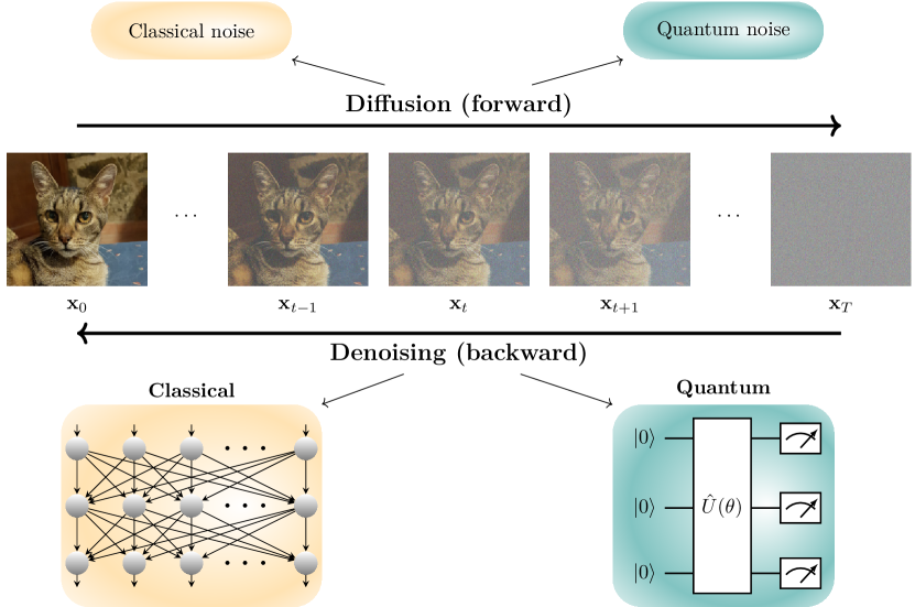
Figure 1: Depiction of the diffusion (from left to right) and denoising (from right to left) processes within a diffusion probabilistic model framework. The original image $\mathbf{x}_{0}$ sampled from the unknown data distribution $p(\mathbf{x}_{0})$ is progressively perturbed ($t\rightarrow t+1$) by adding noise to obtain a latent variable $\mathbf{x}_{T}$ from a known and tractable distribution where the information is completely destroyed. In our framework the diffusion process can be implemented with a classical or a quantum stochastic dynamics. The denoising process is trained to approximate the structure of the data distribution in order to generate new samples. The latter is implemented step by step, using a classical (on the left in blue) or quantum (on the right in orange) parameterized model $\hat{U}(\theta)$ in order to approximate the backward mapping. The standard diffusion models implement both the diffusion and the denoising processes in a classical framework. We propose three different new approaches for the other cases: i) classical diffusion and quantum denoising (CQGDM); ii) quantum diffusion and classical denoising (QCGDM); iii) quantum diffusion and quantum denoising (QQGDM). A similar picture can be applied to time series.

In Machine Learning (ML), diffusion probabilistic models, or briefly Diffusion Models, are an emerging class of generative models used to learn an unknown data distribution in order to produce new data samples. They has been proposed for the first time by Sohl-Dickstein et al. [1] and take inspiration from diffusion phenomena of non-equilibrium statistical physics. The underlying core idea of the DMs is to gradually and slowly destroy the information encoded into the data distribution until it became fully noisy, and then learn how to restore the corrupted information in order to generate new synthetic data. More precisely, the generic structure of diffusion models consists of two stages: (i) a diffusion (or forward) process and (ii) a denoising (or reverse) process. In the former phase, a training data is progressively perturbed by adding noise, typically Gaussian, until all data information is destroyed. The increasing perturbation of information due to the systematically and progressive injections of noise can be physically understood as if the noise propagated inside the data structure, as shown in Fig. 1 from left to right. Let us highlight the fact that in this first stage the training of any ML model is not required. In the second phase, the previous diffusive dynamics is slowly reversed in order to restore the initial data information. The goal of this phase is to learn how to remove noise correctly and produce new data starting from uninformative noise samples as in Fig. 1 from right to left. In contrast to the forward diffusion process, the noise extraction—and as a result the data information retrieval—is implemented training a ML model typically based on a so-called U-Net neural network (NN) architecture [2]. In detail, U-Net models are structured in a succession of convolutional layers followed by an equal number of deconvolutional layers where each deconvolution takes as input the output of the previous deconvolution and also the copy of the output of the corresponding convolutional layer in reverse order. The procedure described above allows DMs to succesfully address the main complication in the design of probabilistic models, i.e., being tractable and flexible at the same time [1, 3]. In fact, alternatively to DMs there are other generative probabilistic models, for instance, Autoregressive Models that are generally tractable but not flexible, or Variational Auto Encoders [4] and Generative Adversarial Networks [5] that are flexible but not tractable.

Diffusion models find use in computer vision for several image processing tasks [6], such as, inpainting [7], super-resolution [8], image-to-image translation [9], and image generation [10, 11, 12]. They are also successfully adopted in several applications, for instance: Stable diffusion [13] that is an open source model for high resolution image syntesis [10]; DALL-E 2 that is a platform implemented by OpenAI [14] to generate photorealistic images from text prompts [11]; Google Imagen [15] that combines transformer language models with diffusion models also in the context of text-to-image generation [12]. Moreover, it has recently been shown that diffusion models perform better than GANs on image synthesis [16].

Furthermore, diffusion models can also be applied to other contexts, for instance in text generation [17, 18] and time-series related tasks [19, 20, 21]. For instance, time series forecasting is the task of predicting future values from past history and diffusion models are employed to generate new samples from the forecasting distribution [22, 23]. Moreover, diffusion models can also be used in time series generation, which is a more complex task involving the complete generation of new time-series samples from a certain distribution [24, 25].

On the other side, very recently, we are witnessing an increasing interest in quantum technologies. Near-term quantum processors are called Noisy Intermediate-Scale Quantum (NISQ) devices [26] and they represent the-state-of-the-art in this context. NISQ computers are engineered with quantum physical systems using different strategies. For instance, a commonly used technology employs superconductive-circuits-based platforms [27, 28] realized with transmon qubits [29, 30]. This technology is exploited, for instance, by IBM [31], Rigetti Computing [32], Google [33]. Moreover D-Wave [34] exploits superconducting integrated circuits mainly as quantum annealers [35]. Xanadu [36] is instead a company employing photons as information units within the linear optical quantum computing paradigm [37] to realize their devices. Finally, the quantum computation can be realized directly manipulating the properties of single atoms. For instance, IonQ [38] realizes quantum devices with trapped ions [39, 40], while Pasqal [41] and QuEra [42] realize analog quantum computers with Rubidium Rydberg neutral atoms held in optical tweezers [43]. All the mentioned devices can be in principle integrated in computational pipelines that can involve also classical computation. In this context they can be referred with the term quantum processing unit (QPU) that can make some computational task much faster than its classical counterpart (CPU) harnessing the quantum properties of particles at the atomic scale. The main reason for building a quantum processor is the possibility of exploiting inherent and peculiar resources of quantum mechanical systems such as superposition and entanglement that, in some cases, allow to perform computational tasks that are impossible or much more difficult via a classic supercomputer [44, 45].

One of the most promising applications of NISQ devices is represented by Quantum Machine Learning (QML) that is a recent interdisciplinary field merging ML and quantum computing, i.e. data to be processed and/or learning algorithms are quantum [46, 47, 48, 44]. Indeed, it involves the integration of ML techniques and quantum computers in order to process and subsequently analyze/learn the underlying data structure. QML can involve the adoption of classical ML methods with quantum data or environments, for instance to analyze noise in quantum devices [49, 50, 51, 52] or to control quantum systems [53]. Alternatively, QML can consider the implementation of novel ML techniques using quantum devices, for instance to implement visual tasks [54] or generative models like Quantum Generative Adversarial Network (QGAN) [55, 56, 57, 58, 59] that are the quantum implementation of classical GAN or in Natural Language Processing (NLP) context to generate text [60]. In fact, quantum devices are capable of processing information in ways that are different from the classical computation. Thus, the implementation of QML models can offer an advantage over the corresponding classical ML models. The latter is expected to arise in the form of quantum speedup or a much smaller number of training parameters, by harness the peculiar properties of quantum systems, for instance, superposition, coherence and entaglement. However, NISQ devices are indeed still very noisy and thus they do not perform the ideal (pure) dynamics. Therefore, the system evolution is affected and driven by quantum noise due to the undesired interactions with external environment and has to be described by the more general open quantum system formalism [61].

In order to generalize DMs with quantum computing ideas, a crucial role is played by noise. In classical information theory, noise is usually modeled by the framework of probability theory, and in general via Markovian processes. Accordingly, the main features of classical noise are a linear relationship among successive steps of the dynamics whose evolution depends only on the current state. Formally, noise is represented by a transition matrix that has the properties of positivity (non-negative entries) and completeness (columns summing to one). In particular, Gaussian noise is a type of random noise that is very often added to the input data of a DM in order to help its learning to generate new data that is as similar as possible to the training data, also in the case when the input is not perfect.

In the quantum domain, noise can be generated also by quantum fluctuations that are typical of quantum systems, hence going much beyond the classical noise sources. Mathematically, quantum noise is described by the more general formalism of quantum operations or quantum maps [61], where, for instance, the decoherence is the typical noise affecting the phase coherence among the quantum states and, in fact, is the main enemy to fight with in order to build up more powerful quantum processors. But what about if such noise is not only detrimental for the quantum computation but it is instead actually very beneficial for some ML tasks as we have observed in the past in other different contexts [62, 63, 53]? Quantum noise might allow, for instance, to generate much more complex (due to the presence of entanglement) probability distributions that would be difficult (or even impossible) to express classically and from which one can sample more efficiently via a quantum processor than via a classical supercomputer.

In this article we therefore introduce and formalize the quantum versions of DMs, particularly based on Denoising Diffusion Probabilistic Models and Score Stochastic Differential Equations in the context of QML. More precisely, we propose three potential quantum-noise-driven generative diffusion models that can be both computationally simulated in the NISQ devices and implemented experimentally due to the naturally occurring noise effects in open quantum systems. The three algorithms are: i) Classical-Quantum Generative Diffusion Model (CQGDM) in which the forward diffusion process can be implemented in the classical way, while the backward denoising with a Quantum Neural Network (QNN) (that can be either a Parametrized Quantum Circuit (PQC) or an hybrid quantum-classical NN); (ii) Quantum-Classical Generative Diffusion Model (QCGDM) in which the noise diffusion process can be implemented in a quantum way, while in the denoising process classical NNs are used; (iii) Quantum-Quantum Generative Diffusion Model (QQGDM) where both the diffusion and the denoising dynamics can be implemented in a quantum domain.

1 Classical-Quantum Generative Diffusion Model (CQGDM)

In this section we propose a model where the diffusion process is classical while the denoising phase is implemented with a quantum dynamics. Moreover, as a result of this setting, the training dataset is necessarily classical, for instance, images, videos, time series, etc.

Formally, given an initial training data $\mathbf{x}_{0}$ sampled from a generic and unknown probability distribution $p(\mathbf{x}_{0})$, the procedure consists in a progressive destruction of the information encoded in the initial data via a diffusive stochastic process. At the end, the data is degraded to a fully noisy state $\mathbf{x}_{T}$ sampled from a classical closed form and tractable prior distribution $p(\mathbf{x}_{T})$ that represents the latent space of the model. Here, tractable stands for the fact that the distribution can be computationally calculated. The implementation of this process can be obtained with different ways. For instance, in DDPM the dynamics of forward diffusive process is implemented by classical Markov chain [1, 3], while in Score SDE the stochastic evolution is determined by a differential equation [64]. In detail, the former approach considers a discrete-time stochastic process whose evolution, at every step, depends only on the previous state and the transition relies on hand-designed kernels $p(\mathbf{x}_{t}|\mathbf{x}_{t-1})$, $t=1,2,\dots,T$ (see Methods for more details). Alternatively, in Score SDE the evolution is a continuous-time process within a close time interval $t\in[0,T]$ and determined by the stochastic differential equation: $\operatorname{\mathrm{d}}\mathbf{x}=\mathbf{f}(\mathbf{x},t)\operatorname{\mathrm{d}}t+g(t)\operatorname{\mathrm{d}}\mathbf{w}$, where $\mathbf{f}(\mathbf{x},t)$ is the drift coefficient, $g(t)$ is the diffusion term, and $\mathbf{w}$ is the Wiener process (also known as standard Brownian motion) that models the stochastic process [65]. The solutions of this equation lead to the tractable prior distribution $p(\mathbf{x}(T))$.

Afterwards, in order to generate new data samples, the objective is to learn how to reverse the diffusion process starting from the prior latent distribution. In case of DDPM, calculating $p(\mathbf{x}_{t-1}|\mathbf{x}_{t})$ is not computationally tractable and it is classically approximated by a model parameterized with $\theta$ (e.g., a NN): $p_{\theta}(\mathbf{x}_{t-1}|\mathbf{x}_{t})$ (see Methods). In the case of Score SDE models, the quantity to be estimated is $\nabla_{\mathbf{x}}\log p_{t}(\mathbf{x})$, where $p_{t}(\mathbf{x})$ is the density probability of $\mathbf{x}(t)$ [64]. Here, for either DDPM and Score SDE diffusion processes, we propose to implement the denoising process with a QNN that can be fully quantum via a PQC or even a classical-quantum hybrid NN model. The results of a simulation of this type of algorithm on a dataset composed of 2-dimensional points distributed along a line segment in the interval $[-1,1]$ is shown in Fig. 2. At the best of our knowledge, this is the first implementation of a hybrid classical-quantum diffusion model, and indeed represents a starting point for more in-depth future studies (for more details on the model and the implementation refer to Section 5.3).

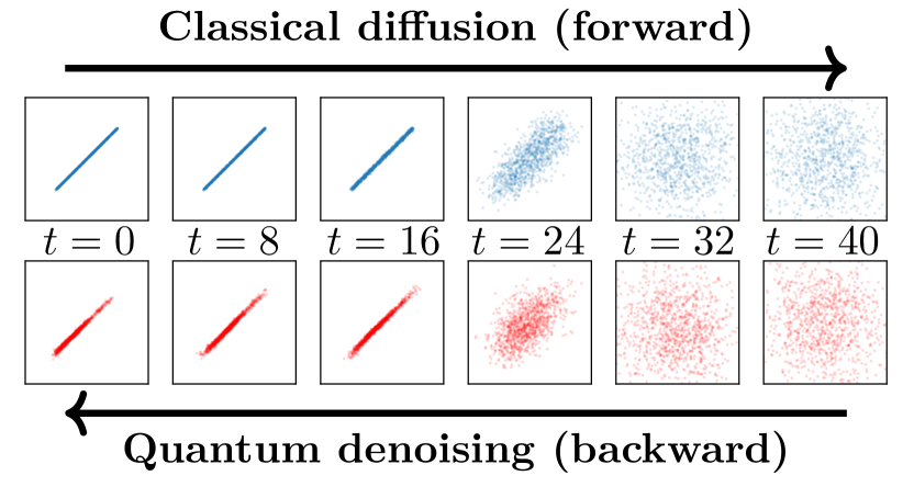
Figure 2: Evolution of the data distribution for a simulated CQGDM. The initial data distribution consists of two-dimensional points distributed in a line segment between $-1$ and $1$. The diffusion process is implemented via a classical DM that transforms the initial data distribution $p(\mathbf{x}_{0})$ at time $t=0$ to the prior $p(\mathbf{x}_{T})$ that is a normalized Gaussian distribution at the final time $t=40$. Meanwhile, the denoising is implemented via a (noiseless) simulated PQC to reconstruct the initial data distribution ($t=0$) from the Gaussian prior ($t=40$). In the top row, we show the forward process (from left to right) for a sample of $1\,000$ points at different discrete time steps $t=0,8,\dots,40$. In the bottom row, we display the denoising (from right to left) of a different sample of $1\,000$ points.

In this context, the main advantage of using the quantum denoising process instead of the classical one can be the possibility of using the trained quantum model to efficiently generate highly dimensional data (e.g., images) taking advantage of the peculiar quantum mechanical properties, such as quantum superposition and entanglement, to speed up data processing [66, 67, 68]. Indeed, QPU devices could be very effective to overcome the main computational burdens of classical diffusion model during this inference process. As shown in Fig. 3, the denoising process for CQGDM crosses the border between classical and quantum distribution spaces, this could take advantage of the quantum speedup in order to accelerate the training of the model.

2 Quantum-Classical Generative Diffusion Model (QCGDM)

In real experiments quantum systems are never perfectly isolated, but they are easily subjected to noise, e.g., interactions with the environment and imperfect implementations. Accordingly, we propose to physically implement the diffusion process via a noisy quantum dynamics exploiting such quantum noise as a positive boost.

In this setting a quantum dataset is considered, i.e., a collection of quantum data. Classical information can be embedded into the initial state of a quantum system, allowing to treat classical data as quantum [48, 69, 70]. Even better, we could avoid the encoding of the classical data if we consider quantum data as any result arising from a quantum experiment [71] or produced directly by a quantum sensing technology [72]. Formally, quantum data is identified with the density operator $\rho(t)$ living in $\mathfrak{S}(\mathcal{H})$ being the set of non-negative operators with unit trace acting on the elements of the Hilbert space $\mathcal{H}$ where the quantum states live.

We here propose two approaches to implement the diffusion process: (i) quantum Markov chains generalizing their classical counterparts [73], and (ii) Stochastic Schrödinger Equation (SSE) [74, 75, 76, 77] modelling the dynamics of an open quantum system subjected to an external noise source.

In the former approach (i), a quantum Markov chain can be described with a composition of transition operation matrices mapping a density operator $\rho$ to another density operator $\rho^{\prime}$. TOMs are matrices whose elements are completely positive maps and whose column sums form a quantum operation (for more details refer to Section 5). A special case of TOMs are the transition effect matrices whose columns are discrete positive operator valued measures. A quantum Markov chains can be, thereby, implemented by a sequence of quantum measurements [73].

The second approach (ii) employs SSEs to describe the physical quantum diffusion process. Given a system in the state $\rho(t)$, its stochastic evolution is determined by a SSE that takes the form $\dot{\rho}(t)=-i[H(t),\rho(t)],$ with $\hbar=1$, and where the Hamiltonian $H(t)=H_{s}(t)+H_{p}(t)$ consists of the sum of the Hamiltonian of the system $H_{s}(t)$ and the stochastic term $H_{p}(t)$ representing the stochastic dynamics to which the quantum system is subjected. Arbitrary sources of noise applied to optimally controlled quantum systems were very recently investigated with the SSEs formalism by our group [78].

The implementation of diffusion dynamics on quantum systems during the forward stage can allow the processing of the data information not only by classically simulated noise but also with quantum physical noise. Here, as previously mentioned, let us remind that quantum noise is more general with respect to its classical counterpart. In particular, the noise distributions used in QCGDMs can be expressed (and more naturally arise by quantum dynamics) in more general and powerful forms respect to the typical Gaussian distributions that are commonly employed in classical DMs. In this set up, at the end of the diffusion process, it is possible to obtain non-classical prior distributions related to entangled state that do not exist in the classical information scenario. In other terms there are probability density distributions that are purely quantum. This can be used to implement diffusion processes that are not possible to be implemented classically. At the end, during the denoising phase, classical NNs can be used in order to remove noise and thus finally generate new samples. Moreover, if the obtained prior distribution is not classical, it is possible to consider the adoption of the denoising NN as a discriminator to identify probability distributions that are purely quantum. This could also be framed in a security context. One can imagine a channel where the communication of data takes place with the application of a quantum diffusion process that maps to a purely quantum probability distribution. In that case, the receiver can restore and so obtain the initial information only with the training of a QNN and thus only with a quantum device. This might be also exploited for quantum attacks/defence in cyber-security applications.

3 Quantum-Quantum Generative Diffusion Model (QQGDM)

In this last section we describe diffusion models within a fully quantum physical framework. Precisely, the training data, the diffusion process and the denoising process have all a quantum mechanical nature. This scenario can be obtained by exploiting the quantum tools described above, namely, quantum Markov chain or SSE for the forward diffusion phase, and a PQC for the backward denoising phase.

Accordingly, all the advantages described in Sections 1 and 2 hold. The adoption of a fully quantum pipeline for both the diffusion and denoising phases would allow the possibility to obtain purely quantum prior distributions that can be processed during the denoising phase with PQCs obtaining a generation process that is not feasible classically. Moreover, this approach could lead to an exponential advantage in sample and time complexity as shown in [72, 79]. As shown in Fig. 3, the diffusion and denoising processes for QQGDM are entirely located in the space of quantum distributions. This might lead to the speedup already described previously for CQGDM and in addition to the possibility of exponentially reducing the computational resources for storing and processing of data information [68]. Finally, it is also possible to access to complex quantum probability distributions that are impossible or much more difficult to treat classically.

4 Discussion

The entanglement is a crucial quantum mechanical phenomenon occurring only in the quantum domain (not classical analogue) when two or more quantum systems interact. It is detected by measurement correlations between the quantum systems that cannot be described with classical physics. Accordingly, quantum systems are capable of representing distributions that are impossible to be produced efficiently with classical computers [80, 46]. For this reason, a quantum diffusion process is capable to explore probability density functions that are not classically tractable.

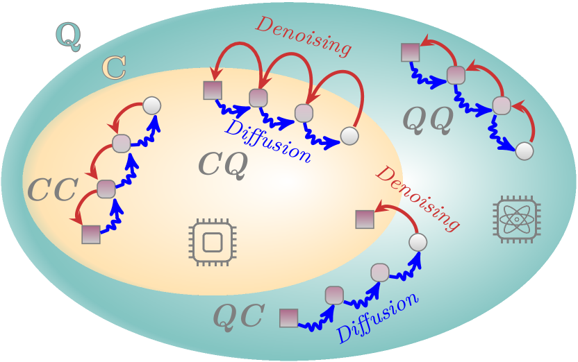
Figure 3: Relationship between the space of the probability distributions that are tractable with classical computation ($\mathbf{C}$) and instead only with quantum computation ($\mathbf{Q}$). We show the trajectories arising from the mappings between probability distributions (colored and white shapes) during the diffusion (blue wavy arrows) and denoising (red arrows) processes for the four different combination: $\mathbf{CC}$, $\mathbf{CQ}$, $\mathbf{QC}$ and $\mathbf{CC}$ indicating whether the diffusion (first letter) and the denoising (second letter) are classical or quantum. The initial data distribution (squares) is progressively transformed during diffusion (changing color and shape) to an uninformative distribution represented by the white circles, and vice versa during denoising. Completely classical models are limited to operate within the space of classically-tractable probability distributions, while completely quantum models can manipulate quantum-tractable probabilities. Models that have classical diffusion and quantum denoising are forced to work only with classical probabilities, but during the denoising phase they can exploit quantum properties within each step. Finally, models that have quantum diffusion and classical denoising can manipulate quantum probabilities during the forward, but in that case, it is not possible to train the classical backward to map those probability distributions.

In Fig. 3 we highlight the relationship between the space of the probability distributions that are tractable with classic computers, which we denote with classical distributions to be more concise, and the space of the probability distributions that are tractable with quantum devices, which we denote with quantum distributions hereinafter. Moreover, we can observe several possible trajectories that map probability distributions to other probability distributions during the diffusion and denoising of the classical DM and of the three proposed quantum approaches: CQGDM, QCGDM and QQGDM.

The classic DM realizes maps from classical distributions to other classical distributions and the NN that implements the denoising are trained to realize the inverse maps, i.e., to match the distributions crossed during the diffusion.

In the CQGDM approach, the diffusion process is implemented classically. Thus, all the probability distributions are necessarily classical. However, during the denoising process, the quantum dynamics is free to explore also the quantum probability space whithin each one of the steps hence exploiting potential (noise-assisted and/or quantum-enhanced) shortcuts. This may give huge advantage for the training of the denoising model. Let us stress that when we evolve quantum systems within a QPU it is possible to process and manipulate exponentially more information as compared to the classical case.

When we consider the fully quantum framework QQGDM we gain the advantage of exploring quantum distributions also during the diffusion phase. For this reason we could explore more complex noisy dynamics compared to the ones that can be simulated in classical computers. Moreover, the two processes can be experimentally implemented on real quantum processors. Furthermore, compared to the CQGDM approach, and provided that the initial distribution of the dataset is quantum, it is possible to design a QQGDM generative models that is capable of generating complex quantum data that are not analytically computable.

Besides, we would like point out that the QCGDM approach can be challenging to be implemented. In detail, if the diffusion process leads to an entagled quantum distribution it is impossible, for the previously mentioned reasons, to efficiently train a classical NN to perform the denoising. This context could be adopted as a proof of concept for the realization of a discriminator for the quantum distributions from the classical ones. In other words, if it is possible to train a model to perform the denoising, then the distribution is classical.

As a future outlook, we would like to realize the implementation of the quantum generative diffusion models either computationally via NISQ and/or physically by using quantum sensing technologies. In particular, regarding QCGDMs and QQGDMs, we propose to implement the diffusion process exploiting naturally noisy quantum dynamics in order to take advantage of the possible benefits of the quantum noise. Instead, regarding CQGDMs and QQGDMs, we propose to use quantum implemented QMLs models, for instance QNNs and PQCs, to learn the denoising process.

Finally, the design and realization of quantum generative diffusion models, with respect to classical DMs, could alleviate and reduce the computational resources (e.g. space of memory, time and energy) to successfully address ML applications such as generation of high-resolution images, the analysis and the prediction of rare events in time-series, and the learning of underlying patterns in experimental data coming also from very different fields as, among others, life and earth science, physics, quantum chemistry, medicine, material science, smart technology engineering, and finance.

5 Methods

In this section we include some mathematical details on the classical and quantum tools for the diffusion and denoising processed discussed in the main text.

5.1 Classical methods

Here we formalize the classical methods used in the standard generative diffusion models and used also for the relevant part of the proposed CQGDM and QCGDM. In particular, we consider classical Markov chains for a Gaussian pertubation and the NNs used for the classical denoising.

The classical diffusion process [1, 3] starts from an initial data sample $\mathbf{x}_{0}$ drawn from an unknown generic distribution $p(\mathbf{x}_{0})$. Gaussian noise is then iteratively injected for a number $T$ of time steps to degrade the data to $\mathbf{x}_{T}$ sampled from a prior Gaussian distribution $\mathcal{N}(0,\mathbf{I})$. In detail, the used Gaussian transition kernel is in the form:

$$p(\mathbf{x}_{t}|\mathbf{x}_{t-1})=\mathcal{N}(\mathbf{x}_{t};\sqrt{1-\beta_{t}}\mathbf{x}_{t-1},\beta_{t}\mathbf{I}),$$ (1)

where $\beta_{t}\in(0,1)$ is an hyperparameter (fixed or scheduled over the time) for the model at the time step $t$ that describes the level of the injected noise, $\beta_{t}\mathbf{I}$ is the identity matrix, and $\mathbf{x}_{t}$ and $\mathbf{x}_{t-1}$ are the random variables at the time steps $t$ and $t-1$, respectively. In this way it is possible to calculate a tractable closed form for the trajectory:

$$p(\mathbf{x}_{1:T}|\mathbf{x}_{0})=p(\mathbf{x}_{0})\prod_{t=1}^{T}p(\mathbf{x}_{t}|\mathbf{x}_{t-1}).$$ (2)

By obing so, for $T$ sufficiently high, $p(\mathbf{x}_{1:T}|\mathbf{x}_{0})$ converges to an isotropic Gaussian $p(\mathbf{x}_{T})=\mathcal{N}(0,\mathbf{I})$. Moreover, given an initial data $\mathbf{x}_{0}$ we can obtain a data sample $\mathbf{x}_{t}$ by sampling a Gaussian vector $\mathbf{\epsilon}\sim\mathcal{N}(0,\mathbf{I})$:

$$\mathbf{x}_{t}=\sqrt{\bar{\alpha}_{t}}\mathbf{x}_{0}+\sqrt{1-\bar{\alpha}_{t}}\mathbf{\epsilon},$$ (3)

where $\alpha_{t}:=1-\beta_{t}$ and $\bar{\alpha}_{t}:=\prod_{s=0}^{t}\alpha_{s}$.

The denoising phase starts from the Gaussian prior distribution and the transition kernel that is implemented is in the form:

$$p_{\theta}(\mathbf{x}_{t}|\mathbf{x}_{t-1})=\mathcal{N}(\mathbf{x}_{t-1};\mathbf{\mu}_{\theta}(\mathbf{x}_{t},t),\mathbf{\Sigma}_{\theta}(\mathbf{x}_{t},t)),$$ (4)

and the closed form for the trajectory is:

$$p_{\theta}(\mathbf{x}_{0:T}|\mathbf{x}_{T})=p(\mathbf{x}_{T})\prod_{t=1}^{T}p_{\theta}(\mathbf{x}_{t-1}|\mathbf{x}_{t}).$$ (5)

Usually, a NN, specifically a U-Net architecture [2], is used to estimate the mean $\mathbf{\mu}_{\theta}(\mathbf{x}_{t},t)$ and the covariance $\mathbf{\Sigma}_{\theta}(\mathbf{x}_{t},t)$ in Eq. 4. In principle, the approach to train the NN would be to find the parameters $\theta$ such that $p_{\theta}(\mathbf{x}_{0})$ would be maximized for each training sample $\mathbf{x}_{0}$. However $p_{\theta}(\mathbf{x}_{0})$ is intractable because it is impossible to marginalize over all the possible trajectories. For this reason, the common approach [3] is to fix the covariance and minimize the loss:

$$\mathcal{L}=\mathbb{E}_{t\sim[1,T]}\mathbb{E}_{\mathbf{x}_{0}\sim p(\mathbf{x}_{0})}\mathbb{E}_{\mathbf{z}_{t}\sim\mathcal{N}(0,\mathbf{I})}||\mathbf{z}_{t}-\mathbf{z}_{\theta}(\mathbf{x}_{t},t)||^{2},$$

where $\mathbf{z}_{t}$ is the real Gaussian noise, and $\mathbf{z}_{\theta}(\mathbf{x}_{t},t)$ is the noise estimation of the model at time $t$.

5.2 Quantum methods

Here we formalize the use of the quantum Markov chain introduced for the diffusion processes of QCGDM and QQGDM in Sections 2 and 3 and the QNNs used for the denoising of CQGDM and QQGDM in Sections 1 and 3.

Formally, a quantum Markov chain can described by two elements: i) a directed graph $G$ whose sites represent the possible state that the quantum system can occupy, ii) a TOM $\mathcal{E}=\mathcal{E}_{ij}$ whose elements are completely positive maps [81, 61] and whose column sums form a quantum operation [73, 44]. Formally, a positive a map is a linear transformation of one positive bounded operator into another. A completely positive map is a linear map $\phi:\mathcal{B(\mathcal{H})}\rightarrow\mathcal{B(\mathcal{H})}$, where $\mathcal{B(\mathcal{H})}$ is the set of bounded linear operators acting on the Hilbert space $\mathcal{H}$, such that the map $\phi\otimes I$ is positive on the space $\mathcal{B(\mathcal{H})}\otimes\mathcal{B(\mathcal{H^{\prime}})}$ for any Hilbert space $\mathcal{H^{\prime}}$. A quantum operation is a completely positive map $\phi$ preserving the trace, i.e., $\tr(\rho)=\tr(\phi(\rho))$, with $\rho\in\mathcal{B(\mathcal{H})}$. Physically, the elements $E_{ij}$ describe the passage operation of the quantum system from site $j$ to site $i$ in one time step. Given a density operator $\rho$, representing the state of system, the quantity $\mathcal{E}(\rho)$ is again a density operator. Moreover, if $\mathcal{E}$ and $\mathcal{F}$ are two TOMs with the same size and acting on the same Hilbert space, then the $\mathcal{EF}$ is again a TOM by matrix multiplication. Accordingly, the dynamics of the quantum system after a discrete number of time steps $n$ is described by the map $\mathcal{E}^{n}=\mathcal{E}\mathcal{E}^{n-1}$, with $n=2,3...$, and the initial state $\rho$ is transformed in the final state $\mathcal{E}^{n}(\rho)$.

Let us now introduce the concepts of QNN [48] in the QML framework and how they are trained. Formally, a QNN can be written as a product of layers of unitary operations:

$$\hat{U}(\mathbf{\theta})=\prod_{\ell=1}^{L}\hat{V}_{\ell}\hat{U}_{\ell}({\mathbf{\theta}_{\ell}}),$$ (6)

where $\hat{V}_{\ell}$ and $\hat{U}_{\ell}({\mathbf{\theta}_{\ell}})$ are fixed and parameterized unitary operations, respectively, for $\ell^{th}$ layer of QNN. The output of the QNN is:

$$f(\mathbf{\theta})=\tr(\mathcal{M}\rho_{\theta})$$ (7)

where $\mathcal{M}$ is an Hermitian operator representing the physical observable, $\rho_{\theta}=\hat{U}(\mathbf{\theta})^{\dagger}\rho_{0}\hat{U}(\mathbf{\theta})$ and $\rho_{0}$ is the initial state, which is the input of the QNN. The QNN is optimized minimizing the difference between its output and the desired value. Generally, the latter is performed with the gradient descent method with the adoption of the parameters shift rule [82].

5.3 Simulation

Here we describe in detail both the model and its implementation regarding the simulation of the CQGDM used to obtain the results of Fig. 2 in Section 1. For the simulation, we used a dataset composed of $1\,000$ points distributed along a line segment in the interval $[-1,1]$.

The diffusion process has been implemented via a classical Markov chain composed of a sequence of Gaussian transition kernels Eq. 1 in order to map the initial data distribution $p(\mathbf{x}_{0})$ to an isotropic Gaussian $p(\mathbf{x}_{T})$ with final time $T\equiv 40$. Furthermore, the data sampling at each time step $t$ is computed by using Eq. 3.

The denoising process has been implemented via a PQC and trained to estimate the mean $\mathbf{\mu}_{\theta}(\mathbf{x}_{t},t)$ and the covariance $\mathbf{\Sigma}_{\theta}(\mathbf{x}_{t},t)$ in Eq. 4. The model is built and simulated with the help of the Pennylane [83] and PyTorch [84] libraries. More precisely, the PQC consist of a four qubits circuit divided in two concatenated parts called head and tail. The parameters of the head are shared among all the values of $t$, while the parameters of the tail are specific for each value of $t=0,\dots,39$. In particular, the head takes as input the values of the coordinates of a single point and encode them in the state of the first two qubits with an angle embedding [48], while the other two qubits are initialized to $\ket{0}$. After the embedding, the circuit is composed of $256$ layers of parametric rotations on the three axes for all the four qubits alternated by layers of entangling controlled not gates [85]. At the end of circuit measurements are performed and the expectation values of the observable $\sigma_{z}$ on all four qubits is computed. The tail is similarly composed, except that the first operation is the angle embedding of the four expectation values previously obtained from the head. In order to simplify the model we assumed that the denoising process is uncorrelated among the features and therefore, the covariance matrix is diagonal and only two values for the variance are necessary. Finally, the four expectation values measured from the tail are used for the predictions of the mean (the first two values) and variance (the second two values). In detail, we multiply the expectation values used for the mean by a factor $3$ in order to enlarge the possible range and the values for the variance are increased by $1$ to force positivity. The model was trained for $40\,000$ epochs on random batches of $1\,000$ points to minimize the Kullback-Leibler divergence between the predicted and desired Gaussian distributions using Adam [86] with learning rate $10^{-4}$. The plots of Fig. 2 are obtained, after the training of the model, using two different random batches of $1\,000$ points, one for the forward and another one for the backward.

References

- \bibcommenthead
- Sohl-Dickstein et al. [2015] Sohl-Dickstein, J., Weiss, E., Maheswaranathan, N., Ganguli, S.: Deep unsupervised learning using nonequilibrium thermodynamics. In: Bach, F., Blei, D. (eds.) Proceedings of the 32nd International Conference on Machine Learning. Proceedings of Machine Learning Research, vol. 37, pp. 2256–2265. PMLR, Lille, France (2015)
- Ronneberger et al. [2015] Ronneberger, O., Fischer, P., Brox, T.: U-net: Convolutional networks for biomedical image segmentation. In: Navab, N., Hornegger, J., Wells, W.M., Frangi, A.F. (eds.) Medical Image Computing and Computer-Assisted Intervention – MICCAI 2015, pp. 234–241. Springer, Cham (2015)
- Ho et al. [2020] Ho, J., Jain, A., Abbeel, P.: Denoising diffusion probabilistic models. In: Larochelle, H., Ranzato, M., Hadsell, R., Balcan, M.F., Lin, H. (eds.) Advances in Neural Information Processing Systems, vol. 33, pp. 6840–6851 (2020)
- Kingma and Welling [2019] Kingma, D.P., Welling, M.: An introduction to variational autoencoders. Foundations and Trends® in Machine Learning 12(4), 307–392 (2019)
- Goodfellow et al. [2020] Goodfellow, I., Pouget-Abadie, J., Mirza, M., Xu, B., Warde-Farley, D., Ozair, S., Courville, A., Bengio, Y.: Generative adversarial networks. Communications of the ACM 63(11), 139–144 (2020)
- Croitoru et al. [2023] Croitoru, F.-A., Hondru, V., Ionescu, R.T., Shah, M.: Diffusion models in vision: A survey. IEEE Transactions on Pattern Analysis and Machine Intelligence, 1–20 (2023)
- Lugmayr et al. [2022] Lugmayr, A., Danelljan, M., Romero, A., Yu, F., Timofte, R., Van Gool, L.: Repaint: Inpainting using denoising diffusion probabilistic models. In: Proceedings of the IEEE/CVF Conference on Computer Vision and Pattern Recognition (CVPR), pp. 11461–11471 (2022)
- Saharia et al. [2023] Saharia, C., Ho, J., Chan, W., Salimans, T., Fleet, D.J., Norouzi, M.: Image super-resolution via iterative refinement. IEEE Transactions on Pattern Analysis and Machine Intelligence 45(4), 4713–4726 (2023)
- Saharia et al. [2022] Saharia, C., Chan, W., Chang, H., Lee, C., Ho, J., Salimans, T., Fleet, D., Norouzi, M.: Palette: Image-to-image diffusion models. In: ACM SIGGRAPH 2022 Conference Proceedings. SIGGRAPH ’22. Association for Computing Machinery, New York, NY, USA (2022)
- Rombach et al. [2022] Rombach, R., Blattmann, A., Lorenz, D., Esser, P., Ommer, B.: High-resolution image synthesis with latent diffusion models. In: Proceedings of the IEEE/CVF Conference on Computer Vision and Pattern Recognition (CVPR), pp. 10684–10695 (2022)
- Ramesh et al. [2022] Ramesh, A., Dhariwal, P., Nichol, A., Chu, C., Chen, M.: Hierarchical text-conditional image generation with clip latents. arXiv e-prints, 2204 (2022)
- Saharia et al. [2022] Saharia, C., Chan, W., Saxena, S., Li, L., Whang, J., Denton, E.L., Ghasemipour, K., Gontijo Lopes, R., Karagol Ayan, B., Salimans, T., et al.: Photorealistic text-to-image diffusion models with deep language understanding. Advances in Neural Information Processing Systems 35, 36479–36494 (2022)
- [13] Stable Diffusion. https://ommer-lab.com/research/latent-diffusion-models
- [14] DALL-E 2. https://openai.com/dall-e-2
- [15] Google Imagen. https://imagen.research.google
- Dhariwal and Nichol [2021] Dhariwal, P., Nichol, A.: Diffusion models beat gans on image synthesis. In: Ranzato, M., Beygelzimer, A., Dauphin, Y., Liang, P.S., Vaughan, J.W. (eds.) Advances in Neural Information Processing Systems, vol. 34, pp. 8780–8794 (2021)
- Savinov et al. [2021] Savinov, N., Chung, J., Binkowski, M., Elsen, E., Oord, A.: Step-unrolled denoising autoencoders for text generation. arXiv e-prints, 2112 (2021)
- Yu et al. [2022] Yu, P., Xie, S., Ma, X., Jia, B., Pang, B., Gao, R., Zhu, Y., Zhu, S.-C., Wu, Y.N.: Latent diffusion energy-based model for interpretable text modelling. In: International Conference on Machine Learning, pp. 25702–25720 (2022). PMLR
- Lin et al. [2023] Lin, L., Li, Z., Li, R., Li, X., Gao, J.: Diffusion models for time series applications: A survey. arXiv e-prints, 2305 (2023)
- Tashiro et al. [2021] Tashiro, Y., Song, J., Song, Y., Ermon, S.: Csdi: Conditional score-based diffusion models for probabilistic time series imputation. In: Ranzato, M., Beygelzimer, A., Dauphin, Y., Liang, P.S., Vaughan, J.W. (eds.) Advances in Neural Information Processing Systems, vol. 34, pp. 24804–24816 (2021)
- Lopez Alcaraz and Strodthoff [2023] Lopez Alcaraz, J.M., Strodthoff, N.: Diffusion-based time series imputation and forecasting with structured state space models. Transactions on machine learning research, 1–36 (2023)
- Rasul et al. [2021] Rasul, K., Seward, C., Schuster, I., Vollgraf, R.: Autoregressive denoising diffusion models for multivariate probabilistic time series forecasting. In: Meila, M., Zhang, T. (eds.) Proceedings of the 38th International Conference on Machine Learning. Proceedings of Machine Learning Research, vol. 139, pp. 8857–8868 (2021)
- Li et al. [2022] Li, Y., Lu, X., Wang, Y., Dou, D.: Generative time series forecasting with diffusion, denoise, and disentanglement. In: Koyejo, S., Mohamed, S., Agarwal, A., Belgrave, D., Cho, K., Oh, A. (eds.) Advances in Neural Information Processing Systems, vol. 35, pp. 23009–23022 (2022)
- Lim et al. [2023] Lim, H., Kim, M., Park, S., Park, N.: Regular time-series generation using sgm. arXiv e-prints, 2301 (2023)
- Adib et al. [2023] Adib, E., Fernandez, A.S., Afghah, F., Prevost, J.J.: Synthetic ecg signal generation using probabilistic diffusion models. IEEE Access (2023)
- Preskill [2018] Preskill, J.: Quantum Computing in the NISQ era and beyond. Quantum 2, 79 (2018)
- Devoret et al. [2004] Devoret, M.H., Wallraff, A., Martinis, J.M.: Superconducting qubits: A short review. arXiv e-prints cond-mat/0411174. (2004)
- Clarke and Wilhelm [2008] Clarke, J., Wilhelm, F.K.: Superconducting quantum bits. Nature 453(7198), 1031–1042 (2008)
- Koch et al. [2007] Koch, J., Yu, T.M., Gambetta, J., Houck, A.A., Schuster, D.I., Majer, J., Blais, A., Devoret, M.H., Girvin, S.M., Schoelkopf, R.J.: Charge-insensitive qubit design derived from the cooper pair box. Phys. Rev. A 76, 042319 (2007)
- Schreier et al. [2008] Schreier, J.A., Houck, A.A., Koch, J., Schuster, D.I., Johnson, B.R., Chow, J.M., Gambetta, J.M., Majer, J., Frunzio, L., Devoret, M.H., Girvin, S.M., Schoelkopf, R.J.: Suppressing charge noise decoherence in superconducting charge qubits. Phys. Rev. B 77, 180502 (2008)
- [31] IBM Quantum Experience. https://quantum-computing.ibm.com
- [32] Rigetti Computing. https://www.rigetti.com
- [33] Google Quantum AI. https://quantumai.google
- [34] D-Wave. https://www.dwavesys.com
- Johnson et al. [2011] Johnson, M.W., Amin, M.H., Gildert, S., Lanting, T., Hamze, F., Dickson, N., Harris, R., Berkley, A.J., Johansson, J., Bunyk, P., et al.: Quantum annealing with manufactured spins. Nature 473(7346), 194–198 (2011)
- [36] Xanadu Quantum Technologies. https://xanadu.ai
- Kok et al. [2007] Kok, P., Munro, W.J., Nemoto, K., Ralph, T.C., Dowling, J.P., Milburn, G.J.: Linear optical quantum computing with photonic qubits. Rev. Mod. Phys. 79, 135–174 (2007)
- [38] IonQ. https://ionq.com
- Allen et al. [2017] Allen, S., Kim, J., Moehring, D.L., Monroe, C.R.: Reconfigurable and programmable ion trap quantum computer. In: 2017 IEEE International Conference on Rebooting Computing (ICRC), pp. 1–3 (2017)
- Monroe and Kim [2013] Monroe, C., Kim, J.: Scaling the ion trap quantum processor. Science 339(6124), 1164–1169 (2013)
- [41] Pasqal. https://www.pasqal.com
- [42] QuEra. https://www.quera.com
- Henriet et al. [2020] Henriet, L., Beguin, L., Signoles, A., Lahaye, T., Browaeys, A., Reymond, G.-O., Jurczak, C.: Quantum computing with neutral atoms. Quantum 4, 327 (2020)
- [44] Nielsen, M.A., Chuang, I.L.: Quantum Computation and Quantum Information. Cambridge university press (2010)
- Feynman [1982] Feynman, R.P.: Simulating physics with computers. International Journal of Theoretical Physics 21 (1982)
- Biamonte et al. [2017] Biamonte, J., Wittek, P., Pancotti, N., Rebentrost, P., Wiebe, N., Lloyd, S.: Quantum machine learning. Nature 549(7671), 195–202 (2017)
- [47] Wittek, P.: Quantum Machine Learning: What Quantum Computing Means to Data Mining. Academic Press (2014)
- [48] Schuld, M., Petruccione, F.: Machine Learning with Quantum Computers. Springer
- Canonici et al. [2023] Canonici, E., Martina, S., Mengoni, R., Ottaviani, D., Caruso, F.: Machine-learning based noise characterization and correction on neutral atoms nisq devices. arXiv e-prints, 2306 (2023)
- Martina et al. [2023a] Martina, S., Hernández-Gómez, S., Gherardini, S., Caruso, F., Fabbri, N.: Deep learning enhanced noise spectroscopy of a spin qubit environment. Machine Learning: Science and Technology 4(2), 02–01 (2023)
- Martina et al. [2023b] Martina, S., Gherardini, S., Caruso, F.: Machine learning classification of non-markovian noise disturbing quantum dynamics. Physica Scripta 98(3), 035104 (2023)
- Martina et al. [2022] Martina, S., Buffoni, L., Gherardini, S., Caruso, F.: Learning the noise fingerprint of quantum devices. Quantum Machine Intelligence 4(1), 8 (2022)
- Dalla Pozza et al. [2022] Dalla Pozza, N., Buffoni, L., Martina, S., Caruso, F.: Quantum reinforcement learning: the maze problem. Quantum Machine Intelligence 4(1), 11 (2022)
- Das et al. [2023] Das, S., Zhang, J., Martina, S., Suter, D., Caruso, F.: Quantum pattern recognition on real quantum processing units. Quantum Machine Intelligence 5(1), 16 (2023)
- Lloyd and Weedbrook [2018] Lloyd, S., Weedbrook, C.: Quantum generative adversarial learning. Phys. Rev. Lett. 121, 040502 (2018)
- Dallaire-Demers and Killoran [2018] Dallaire-Demers, P.-L., Killoran, N.: Quantum generative adversarial networks. Phys. Rev. A 98, 012324 (2018)
- Zoufal et al. [2019] Zoufal, C., Lucchi, A., Woerner, S.: Quantum generative adversarial networks for learning and loading random distributions. npj Quantum Information 5(1), 103 (2019)
- Braccia et al. [2021] Braccia, P., Caruso, F., Banchi, L.: How to enhance quantum generative adversarial learning of noisy information. New Journal of Physics 23(5), 053024 (2021)
- Braccia et al. [2022] Braccia, P., Banchi, L., Caruso, F.: Quantum noise sensing by generating fake noise. Phys. Rev. Appl. 17, 024002 (2022)
- Karamlou et al. [2022] Karamlou, A., Wootton, J., Pfaffhauser, M.: Quantum natural language generation on near-term devices. In: Proceedings of the 15th International Conference on Natural Language Generation, pp. 267–277 (2022)
- Caruso et al. [2014] Caruso, F., Giovannetti, V., Lupo, C., Mancini, S.: Quantum channels and memory effects. Rev. Mod. Phys. 86, 1203–1259 (2014)
- Caruso et al. [2010] Caruso, F., Huelga, S.F., Plenio, M.B.: Noise-enhanced classical and quantum capacities in communication networks. Phys. Rev. Lett. 105, 190501 (2010)
- Caruso et al. [2016] Caruso, F., Crespi, A., Ciriolo, A.G., Sciarrino, F., Osellame, R.: Fast escape of a quantum walker from an integrated photonic maze. Nature communications 7(1), 11682 (2016)
- Song et al. [2021] Song, Y., Sohl-Dickstein, J., Kingma, D.P., Kumar, A., Ermon, S., Poole, B.: Score-based generative modeling through stochastic differential equations. In: International Conference on Learning Representations (2021)
- Yang et al. [2022] Yang, L., Zhang, Z., Hong, S., Zhang, W.: Diffusion models: A comprehensive survey of methods and applications. arXiv e-prints, 2209 (2022)
- Lloyd et al. [2014] Lloyd, S., Mohseni, M., Rebentrost, P.: Quantum principal component analysis. Nature Physics 10(9), 631–633 (2014)
- Wiebe et al. [2012] Wiebe, N., Braun, D., Lloyd, S.: Quantum algorithm for data fitting. Phys. Rev. Lett. 109, 050505 (2012)
- Yao et al. [2017] Yao, X.-W., Wang, H., Liao, Z., Chen, M.-C., Pan, J., Li, J., Zhang, K., Lin, X., Wang, Z., Luo, Z., Zheng, W., Li, J., Zhao, M., Peng, X., Suter, D.: Quantum image processing and its application to edge detection: Theory and experiment. Phys. Rev. X 7, 031041 (2017)
- Lloyd et al. [2020] Lloyd, S., Schuld, M., Ijaz, A., Izaac, J., Killoran, N.: Quantum embeddings for machine learning. arXiv e-prints, 2001 (2020)
- Gianani et al. [2022] Gianani, I., Mastroserio, I., Buffoni, L., Bruno, N., Donati, L., Cimini, V., Barbieri, M., Cataliotti, F.S., Caruso, F.: Experimental quantum embedding for machine learning. Advanced Quantum Technologies 5(8), 2100140 (2022)
- Huang et al. [2021a] Huang, H.-Y., Broughton, M., Mohseni, M., Babbush, R., Boixo, S., Neven, H., McClean, J.R.: Power of data in quantum machine learning. Nature communications 12(1), 2631 (2021)
- Huang et al. [2021b] Huang, H.-Y., Kueng, R., Preskill, J.: Information-theoretic bounds on quantum advantage in machine learning. Phys. Rev. Lett. 126, 190505 (2021)
- Gudder [2008] Gudder, S.: Quantum Markov chains. Journal of Mathematical Physics 49(7) (2008). 072105
- Davies and Lewis [1970] Davies, E.B., Lewis, J.T.: An operational approach to quantum probability. Communications in Mathematical Physics 17(3), 239–260 (1970)
- Wiseman [1996] Wiseman, H.M.: Quantum trajectories and quantum measurement theory. Quantum and Semiclassical Optics: Journal of the European Optical Society Part B 8(1), 205 (1996)
- [76] Breuer, H.-P., Petruccione, F.: The Theory of Open Quantum Systems. Oxford University Press (2002)
- Rivas and Huelga [Springer, 2012] Rivas, A., Huelga, S.F.: Open Quantum Systems vol. 10, (Springer, 2012)
- Müller et al. [2022] Müller, M.M., Gherardini, S., Calarco, T., Montangero, S., Caruso, F.: Information theoretical limits for quantum optimal control solutions: error scaling of noisy control channels. Scientific Reports 12(1), 21405 (2022)
- Aharonov et al. [2022] Aharonov, D., Cotler, J., Qi, X.-L.: Quantum algorithmic measurement. Nature communications 13(1), 887 (2022)
- Bouland et al. [2019] Bouland, A., Fefferman, B., Nirkhe, C., Vazirani, U.: On the complexity and verification of quantum random circuit sampling. Nature Physics 15(2), 159–163 (2019)
- Lindblad [1975] Lindblad, G.: Completely positive maps and entropy inequalities. Communications in Mathematical Physics 40, 147–151 (1975)
- Schuld et al. [2019] Schuld, M., Bergholm, V., Gogolin, C., Izaac, J., Killoran, N.: Evaluating analytic gradients on quantum hardware. Phys. Rev. A 99, 032331 (2019)
- Bergholm et al. [2022] Bergholm, V., Izaac, J., Schuld, M., Gogolin, C., Ahmed, S., Ajith, V., Alam, M.S., Alonso-Linaje, G., AkashNarayanan, B., Asadi, A., Arrazola, J.M., Azad, U., Banning, S., Blank, C., Bromley, T.R., Cordier, B.A., Ceroni, J., Delgado, A., Matteo, O.D., Dusko, A., Garg, T., Guala, D., Hayes, A., Hill, R., Ijaz, A., Isacsson, T., Ittah, D., Jahangiri, S., Jain, P., Jiang, E., Khandelwal, A., Kottmann, K., Lang, R.A., Lee, C., Loke, T., Lowe, A., McKiernan, K., Meyer, J.J., Montañez-Barrera, J.A., Moyard, R., Niu, Z., O’Riordan, L.J., Oud, S., Panigrahi, A., Park, C.-Y., Polatajko, D., Quesada, N., Roberts, C., Sá, N., Schoch, I., Shi, B., Shu, S., Sim, S., Singh, A., Strandberg, I., Soni, J., Száva, A., Thabet, S., Vargas-Hernández, R.A., Vincent, T., Vitucci, N., Weber, M., Wierichs, D., Wiersema, R., Willmann, M., Wong, V., Zhang, S., Killoran, N.: PennyLane: Automatic differentiation of hybrid quantum-classical computations (2022)
- Paszke et al. [2019] Paszke, A., Gross, S., Massa, F., Lerer, A., Bradbury, J., Chanan, G., Killeen, T., Lin, Z., Gimelshein, N., Antiga, L., et al.: Pytorch: An imperative style, high-performance deep learning library. Advances in neural information processing systems 32 (2019)
- Schuld et al. [2020] Schuld, M., Bocharov, A., Svore, K.M., Wiebe, N.: Circuit-centric quantum classifiers. Phys. Rev. A 101, 032308 (2020)
- Kingma and Ba [2017] Kingma, D.P., Ba, J.: Adam: A Method for Stochastic Optimization (2017)