Delay Update in Determinant Quantum Monte Carlo

Abstract

Determinant quantum Monte Carlo (DQMC) is a widely used unbiased numerical method for simulating strongly correlated electron systems. However, the update process in DQMC is often a bottleneck for its efficiency. To address this issue, we propose a generalized delay update scheme that can handle both onsite and extended interactions. Our delay update scheme can be implemented in both zero-temperature and finite-temperature versions of DQMC. We apply the delay update scheme to various strongly correlated electron models and evaluate its efficiency under different conditions. Our results demonstrate that the proposed delay update scheme significantly improves the efficiency of DQMC simulations, enable it to simulate larger system size.

I Introduction

Strongly correlated electron systems have garnered significant attention in past decades. These systems exhibit a rich variety of phases, such as high-temperature superconductivity [1, 2, 3, 4, 5], fractional quantum Hall [6, 7, 8, 9], quantum spin liquids [10, 11, 12, 13, 14, 15, 14] and so on. Their study has led to a deeper understanding of the underlying profound physics governing their behavior. Due to non-perturbative nature of strongly correlated electron systems, it requires the development of advanced, unbiased simulation methods to accurately study their properties.

Determinant Quantum Monte Carlo (DQMC) [16, 17, 18, 19, 20, 21, 22, 23, 24] has emerged as a powerful and widely-used technique for simulating strongly correlated electrons, providing crucial insights into the behavior of these systems. This method has been successfully applied to a variety of interesting models, enabling researchers to explore novel phases and phase transitions [25, 26, 27, 28, 29, 30, 31, 32, 33, 34, 35, 36, 37, 38, 39, 40, 41, 42, 43, 44, 45, 46, 47, 48, 49, 50, 51, 52]. However, despite its many successes, DQMC is not without its limitations, even if we only focus on sign-problem-free models. Due to the inherently high computational complexity associated with this approach, simulations are typically restricted to relatively small system sizes. This limitation restricts our ability to accurately extrapolate to the thermodynamic limit, which is necessary to determine the properties of phases and phase transitions with greater accuracy.

The computational complexity of DQMC primarily arises from the need to update and manipulate large Green’s function matrices during the simulation process. In DQMC, we use Trotter decomposition such that the inverse temperature $\beta$ is divided into many small slices (e.g. $\beta=L_{\tau}\Delta_{\tau}$, where $\Delta_{\tau}$ is a small imaginary time slice, $L_{\tau}$ is the total number of imaginary time slices), and Hubbard stratonovich (HS) transformation is used to decouple interaction term by introducing auxiliary fields. We usually need $\mathcal{O}(\beta N)$ number of auxiliary fields, where $N$ is the number of system size. The Boltzmann weight for each configuration involves a determinant of Green’s function matrix. Direct calculation of the determinant ratio and the updated Green’s function has the computational complexity of $\mathcal{O}(N^{3})$. In DQMC, we use local update, and for models with local interactions, the Green’s function before and after local update only differs by a low-rank update which can be performed by using the Sherman-Morrison formula and it reduces complexity of calculation determinant ratio to $\mathcal{O}(1)$ and reduce complexity of calculation of updated Green’s function to $\mathcal{O}(N^{2})$. This low-rank update is also called fast update. Therefore, for DQMC simulation of models with local interaction, one Monte Carlo step (which is defined as a whole sweep of all auxiliary fields, and we call a whole sweep of all auxiliary fields as a sweep in this work.) has the computational complexity of $\mathcal{O}(\beta N^{3})$, while for models with long range interactions [50, 51], this complexity is $\mathcal{O}(\beta N^{4})$. The latter situation is relatively rare and is not within the scope of our consideration in this article.

It was pointed out that successive low-rank update of whole Green’s function after each local update can be delayed as the determinant ratio calculation only requires diagonal part of the Green’s function [53, 54]. This is the so called delay update. In delay update, after each local update, one only keeps updating the diagonal part of the Green’s function and record some intermediate vectors which will be useful in the final update of the whole Green’s function. The delay update has been successfully implemented in Hirsch-Fye QMC [53, 54] and continuous-time QMC [55], and it can significantly reduce the prefactor of total computational complexity. However, those implementation only consider finite temperature and onsite interactions, how to generalize it to multi-site extended interactions and zero-temperature remains an incomplete task. In this work, we consider general cases where local update involve $k$-rank update, such that it can apply to general strongly correlated electron models with extended interactions. We implement the general delay update in the framework of DQMC both in the finite and zero-temperature versions. The general delay update can be generalized to Hirsch-Fye QMC and continuous-time QMC straightforwardly.

The remain part of the article is organized as follows. In Sec. II, we introduce the basic formalism of delay update. In Sec. III, we compare the efficiency of delay update with conventional fast update on both Hubbard model and spinless $t$-$V$ model on a two dimensional square lattice. At last we make a brief conclusion and discussion in Sec. IV.

II Method

Before introducing the basic formalism of generalized delay update, we review the fast update first [16, 17, 18, 19, 20, 21, 22, 23, 24]. Without loss of generality, we first consider finite temperature version of DQMC (DQMC-finite-T), and discuss zero-temperature case only when it is necessary. In DQMC, interacting fermion problem is mapped to a non-interacting fermion problem coupling to auxiliary fields (${\bm{s}}$), take the Hubbard model [56, 57, 58, 59] as an example, with Hamiltonian

$$H_{tU}=H_{0}+H_{U}$$ (1)

where $H_{0}=-t\sum_{\langle i,j\rangle,\alpha}(c_{i,\alpha}^{\dagger}c_{j,\alpha}+\text{H.c.})$ and $H_{U}=\frac{U}{2}\sum_{i}(n_{i}-1)^{2}$. In the Hamiltonian, $c_{i,\alpha}^{\dagger}$ creates an electron on site $i$ with spin polarization $\alpha=\uparrow/\downarrow$, $n_{i}=\sum_{\alpha}c_{i\alpha}^{\dagger}c_{i\alpha}$ is the fermion number density operator, $t$ is the nearest-neighbour (NN) hopping term, and $U$ is the amplitude of onsite Hubbard repulsive interaction. In this work, we use following HS transformation

$$e^{-\Delta_{\tau}\frac{U}{2}\sum_{i}(n_{i}-1)^{2}}$$ (2)

$$= \frac{1}{4}\sum_{\bm{s}_{i,l}=\pm 1,\pm 2}\gamma(\bm{s}_{i,l})e^{-i\alpha_{U}\sum_{i}\eta(\bm{s}_{i,l})(n_{i}-1)}+O(\Delta_{\tau}^{4})$$

where $\bm{s}_{i,l}$ is auxiliary field, $\alpha_{U}=\sqrt{\Delta_{\tau}U}$, $\gamma(\pm 1)=1+\frac{\sqrt{6}}{3}$, $\gamma(\pm 2)=1-\frac{\sqrt{6}}{3}$, $\eta(\pm 1)=\pm\sqrt{2(3-\sqrt{6})}$, $\eta(\pm 2)=\pm\sqrt{2(3+\sqrt{6})}$. After Trotter decomposition and HS transformation, and fermion degrees of freedom can be easily traced out, so the partition function becomes

$$Z=\sum_{\bm{s}}w_{b}[\bm{s}]w_{f}[\bm{s}]$$ (3)

where we denote all auxiliary fields $\{\bm{s}_{i,l}\}$ as $\bm{s}$, and defined the scalar weight

$$w_{b}\left[\bm{s}\right]\equiv\prod_{i,l}(\gamma(\bm{s}_{i,l})e^{-i\alpha_{U}\eta(\bm{s}_{i,l})})$$ (4)

and the determinant weight

$$w_{f}\left[\bm{s}\right]=\det\left[I+B_{\bm{s}}(\beta,0)\right].$$ (5)

$B_{\bm{s}}(\beta,0)$ is called the time evolution matrix, and the general time evolution matrix $B(\tau_{2},\tau_{1})$ ($\tau_{2}\geq\tau_{1}$) is defined as

$$B_{\bm{s}}(\tau_{2},\tau_{1})=B_{\bm{s}}^{l_{2}}B_{\bm{s}}^{l_{2}-1}\cdots B_{\bm{s}}^{l_{1}+1}$$ (6)

where $\tau_{2}=l_{2}\Delta_{\tau}$, $\tau_{1}=l_{1}\Delta_{\tau}$, and $B^{l}_{\bm{s}}=e^{V({\bm{s}})}e^{-\Delta_{\tau}K}$, where $K$ is the coefficient matrix for non-interacting part of the Hamiltonian $H_{0}=\sum_{j,k}c_{j}^{\dagger}K_{j,k}c_{k}=\bm{c}^{\dagger}K\bm{c}$, and $V({\bm{s}})$ is the coefficient matrix for interacting part after HS transformation, $i\alpha_{U}\sum_{i}\eta(\bm{s})n_{i}=\sum_{j,k}c_{j}^{\dagger}V(\bm{s})_{j,k}c_{k}=\bm{c}^{\dagger}V(\bm{s})\bm{c}$. Note that we have absorbed the spin index into site index for convenient. Above formalism directly applies to general interacting models, so in the following, we will not limited to Hubbard model, but consider general interactions which may have extended interactions.

Consider a local update of $\bm{s}$, which only changes certain component $\bm{s}_{i,l}$ and we denote its effect on the change of $e^{V({\bm{s}}_{i,l})}$ as $\Delta=e^{V({\bm{s^{\prime}}})}e^{-V({\bm{s}})}-I$, then the determinant ratio can be calculated as

$$\frac{w_{f}[\bm{s}^{\prime}]}{w_{f}[\bm{s}]}=\det\left[I+\Delta(I-G(\tau,\tau))\right]$$ (7)

where the equal-time Green’s function is a matrix with the elements $G_{ij}(\tau,\tau)\equiv\langle c_{i}(\tau)c_{j}^{\dagger}(\tau)\rangle$, and $G(\tau,\tau)$ can be calculated as [16, 17, 18, 19, 20, 21, 22, 23, 24]

$$G(\tau,\tau)=\left(I+B(\tau,0)B(\beta,\tau)\right)^{-1}$$ (8)

To keep the notation succinct, we will omit the subscript ${\bm{s}}$ for both $G$ and $B$ matrices when necessary. We assume $\Delta$ is a sparse matrix with only $k$ non-zero elements and they are all in the diagonal. We can obtain this form usually for local interactions. We denote the position of $k$ non-zero elements as $x_{1}$, $x_{2}$ $\cdots$ $x_{k}$. Due to the sparse nature of $\Delta$, the determinant ratio can be simplified to

$$\frac{w_{f}[\bm{s}^{\prime}]}{w_{f}[\bm{s}]}=\det\left[S\right]$$ (9)

with $S$ only a $k$-dimension matrix

$$S=I_{k\times k}+\mathcal{V}D.$$ (10)

where $I_{k\times k}$ is the $k$-dimension identity matrix, $\mathcal{V}$ and $D$ are $k$-dimension matrices written as

$$\mathcal{V}=\left[\begin{array}[]{ccc}-(G_{x_{1}x_{1}}-1)&-G_{x_{1}x_{2}}&\cdots\\ -G_{x_{2}x_{1}}&-(G_{x_{2}x_{2}}-1)&\cdots\\ \vdots&\vdots&\ddots\end{array}\right]_{k\times k}$$ (11)

$$D=\left[\begin{array}[]{ccc}\Delta_{x_{1}x_{1}}\\ &\Delta_{x_{2}x_{2}}\\ &&\ddots\end{array}\right]_{k\times k}$$ (12)

If the update is accepted, in the fast update scheme, the Green’s function will be updated

$$G^{\prime}=G+\mathbb{U}\mathbb{S}\mathbb{V}$$ (13)

with

$$\mathbb{U} =[G_{:,x_{1}}|G_{:,x_{2}}|\cdots]_{N\times k}$$ (14)

$$\mathbb{S}=DS^{-1}$$ (15)

$$\mathbb{V}=\left(\left[G_{x_{1},:}-e_{x_{1}}|G_{x_{2},:}-e_{x_{2}}|\cdots\right]^{T}\right)_{k\times N}$$ (16)

where $e_{x_{j}}$ denotes a row vector with only one non-zero element at position $x_{j}$, $G_{:,x_{j}}$ denotes column $x_{j}$ of $G$, and $G_{x_{j},:}$ denotes row $x_{j}$ of $G$.

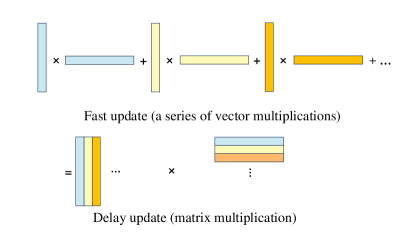
Figure 1: The schematic diagram of delay update. Compared to fast update, delay update transforms a series of vector multiplications into matrix multiplications.

As we can see in Eqs. (9-12), the determinant ratio only involves very small part of Green’s function, the delay update scheme applies. In delay update, we only update the whole Green’s function occasionally. After each local update, we will collect $\mathbb{U}$, $\mathbb{S}$ and $\mathbb{V}$ matrices, and use them to update the whole Green’s function after certain number of $\mathbb{U}$, $\mathbb{S}$ and $\mathbb{V}$ matrices are collected. We denote this number as $n_{d}$.

Let us consider the delay update step by step. At the beginning, we have the initial $G^{(0)}$ and use it to calculate $S^{(1)}$, then the determinant ratio is $\det(S^{(1)})$. If the update is accepted, calculate $D^{(1)}$, $\mathbb{U}^{(1)}$, $\mathbb{S}^{(1)}$ and $\mathbb{V}^{(1)}$. Assume we already accepted $i-1<n_{d}$ times, namely, we have stored $\{\mathbb{U}^{(1)},\cdots,\mathbb{U}^{(i-1)}\}$, $\{\mathbb{S}^{(1)},\cdots,\mathbb{S}^{(i-1)}\}$ and $\{\mathbb{V}^{(1)},\cdots,\mathbb{V}^{(i-1)}\}$, now we consider $i$-th step, and give following recurrence relations. At $i$-th step, we calculate

$$S^{(i)}=I_{k\times k}+\mathcal{V}^{(i)}D^{(i)}$$ (17)

with

$$\mathcal{V}^{(i)}=\left[\begin{array}[]{ccc}-(G_{x_{1}^{(i)}x_{1}^{(i)}}^{(i-1)}-1)&-G_{x_{1}^{(i)}x_{2}^{(i)}}^{(i-1)}&\cdots\\ -G_{x_{2}^{(i)}x_{1}^{(i)}}^{(i-1)}&-(G_{x_{2}^{(i)}x_{2}^{(i)}}^{(i-1)}-1)&\cdots\\ \vdots&\vdots&\ddots\end{array}\right]_{k\times k}$$ (18)

$$D^{(i)}=\left[\begin{array}[]{ccc}\Delta_{x_{1}^{(i)}x_{1}^{(i)}}&0&\cdots\\ 0&\Delta_{x_{2}^{(i)}x_{2}^{(i)}}&\cdots\\ \vdots&\vdots&\ddots\end{array}\right]_{k\times k}$$ (19)

The determinant ratio is $\det\left[S^{(i)}\right]$. If the update is accepted, we calculate

$$\mathbb{U}^{(i)} =[G_{:,x_{1}^{(i)}}^{(i-1)}|G_{:,x_{2}^{(i)}}^{(i-1)}|\cdots]_{N\times k}$$ (20)

$$\mathbb{S}^{(i)}=D^{(i)}\left(S^{(i)}\right)^{-1}$$ (21)

$$\mathbb{V}^{(i)}=\left(\left[G_{x_{1}^{(i)},:}^{(i-1)}-e_{x_{1}^{(i)}}|G_{x_{2}^{(i)},:}^{(i-1)}-e_{x_{2}^{(i)}}|\cdots\right]^{T}\right)_{k\times N}$$ (22)

where $e_{x_{j}^{(i)}}$ denotes a row vector with only one non-zero element at position $x_{j}^{(i)}$, $G_{:,x_{j}^{(i)}}^{(i-1)}$ denotes column $x_{j}^{(i)}$ of $G^{(i-1)}$, and $G_{x_{j}^{(i)},:}^{(i-1)}$ denotes row $x_{j}^{(i)}$ of $G^{(i-1)}$. In above, we will calculate part of the Green’s function before the $i$-th step update with following formulas,

$$G_{:,x_{j}^{(i)}}^{(i-1)}=G_{:,x_{j}^{(i)}}^{(0)}+\sum_{m=1}^{i-1}\mathbb{U}_{:,\mu}^{(m)}\mathbb{S}_{\mu\nu}^{(m)}\mathbb{V}_{\nu x_{j}^{(i)}}^{(m)}$$ (23)

$$G_{x_{j}^{(i)},:}^{(i-1)}=G_{x_{j}^{(i)},:}^{(0)}+\sum_{m=1}^{i-1}\mathbb{U}_{x_{j}^{(i)}\mu}^{(m)}\mathbb{S}_{\mu\nu}^{(m)}\mathbb{V}_{\nu,:}^{(m)}$$ (24)

where $j=1,2,\cdots,k$.

After $n_{d}$-steps,we update the whole Green’s function

$$G^{(n_{d})}=G^{(0)}+\sum_{m=1}^{n_{d}}\mathbb{U}^{(m)}\mathbb{S}^{(m)}\mathbb{V}^{(m)}$$ (25)

This can be done by matrix product. Here we make a brief discussion about the computational complexity for delay update. The total overhead for preparing the intermediate matrices mainly comes from calculating part of the Green’s function, which has the computational complexity $\mathcal{O}(n_{d}^{2}N)$, and after $n_{d}$ steps, the calculation of the whole Green’s function cost $\mathcal{O}(n_{d}N^{2})$. By going through all auxiliary fields, we need multiply above complexity by a factor $\mathcal{O}(\beta N/n_{d})$, so that we have $\mathcal{O}(\beta n_{d}N^{2})$ for overhead, and $\mathcal{O}(\beta N^{3})$ for Green’s function updates. It is obvious that delay update and fast update share the same computational complexity. However, in delay update a series of vector outer-products are transformed into matrix products as shown in Fig. 1. The whole Green’s function is updated occasionally, which makes a much better use of cache. The chosen of parameter $n_{d}$ can be based on some test, and we find by setting $n_{d}$ to $2^{\lambda}$ with $\lambda=\min[6,[\log_{2}\frac{N}{20}]]$ is a good choice, e.g., for $N=42^{2}$, $n_{d}$ can be set to 64.

The above delay update scheme can also be applied to zero-temperature version of DQMC. For zero-temperature version of DQMC (DQMC-zero-T), the normalization factor of ground state wavefunction $|\Psi_{0}\rangle$ plays the similar role of partition function for finite-temperature case.

$$\langle\Psi_{0}|\Psi_{0}\rangle=\sum_{\bm{s}}\det\left[P^{\dagger}B_{\bm{s}}(2\Theta,0)P\right]$$ (26)

where $|\Psi_{0}\rangle=e^{-\Theta H}|\Psi_{T}\rangle$ is obtained by projection on a trial wavefunction $|\Psi_{T}\rangle=\prod_{i=1}^{N_{\text{p}}}({\bm{c}}^{\dagger}P)_{i}|0\rangle$, $\Theta$ is the projection time, $N_{\text{p}}$ is the number of particles, and $P$ is a matrix with a dimension of $N\times N_{\text{p}}$. Usually, we choose the trial wavefunction as the ground state of non-interacting part $H_{0}=\bm{c}^{\dagger}K\bm{c}$, and then $P$ is composed of $N_{\text{p}}$ lowest eigenvectors of $K$. To keep a consistent notation with finite temperature case, we will use $2\Theta$ and $\beta$ interchangeably when necessary. In zero-temperature case, we usually define $B^{\rangle}(\tau)=B(\tau,0)P$ and $B^{\langle}(\tau)=P^{\dagger}B(2\Theta,\tau)$. In fast update of zero-temperature DQMC, we keep track of $B^{\langle}(\tau)$, $B^{\rangle}(\tau)$ and $\left(B^{\langle}(\tau)B^{\rangle}(\tau)\right)^{-1}$ instead of Green’s function. After each local update, $B^{\rangle}(\tau)$ is changed to $(I+\Delta)B^{\rangle}(\tau)$, and the formula to calculate the determinant ratio is similar to the finite temperature case. If the update is accepted, we update $B^{\rangle}(\tau)$ and $\left(B^{\langle}(\tau)B^{\rangle}(\tau)\right)^{-1}$. The computation complexity is $\mathcal{O}(\beta NN_{\text{p}}^{2})$. To apply delay update to zero-temperature case, it will be more convenient to work with Green’s function instead of $B^{\langle}(\tau)$, $B^{\rangle}(\tau)$ and $\left(B^{\langle}(\tau)B^{\rangle}(\tau)\right)^{-1}$. In zero-temperature DQMC, we calculate Green’s function with

$$G(\tau,\tau)=I-B^{\rangle}(\tau)\left(B^{\langle}(\tau)B^{\rangle}(\tau)\right)^{-1}B^{\langle}(\tau).$$ (27)

Based on Green’s function, the delay update formula for zero-temperature case is quite similar to finite-temperature case, but also has a little difference. At the beginning of local update in each time slices, we have to calculate the Green’s function using Eq. (27). Note that computational complexity of delay update based on Green’s function is $\mathcal{O}(\beta N^{3})$, which is greater than $\mathcal{O}(\beta NN_{\text{p}}^{2})$. To possibly gain better performance than fast update for zero-temperature case, we require $N_{\text{p}}$ to be comparable to $N$, which is usually the case we considered in strongly correlated electron lattice models.

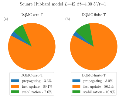
Figure 2: The proportion of total computation time occupied by each process in a DQMC calculation of Hubbard model on a square lattice. The figure shows computation time of system size $42\times 42$ with model parameters $\beta t=4$ and $U/t=1$ .(a) The proportion of each process in DQMC-zero-T. (b) The proportion of each process in DQMC-finite-T. The blue zone is propagation of the Green’s function, the orange zone is fast updates and the green zone is numerical stabilization

III Model and result

To show the speedup of delay update over fast update in DQMC, let us first consider there is only one non-zero diagonal element in $\Delta$ ($k=1$), we first apply delay update to the Hubbard model [56, 57, 58, 59] on square lattice,

$$H_{tU}=-t\sum_{\langle i,j\rangle,\alpha}(c_{i,\alpha}^{\dagger}c_{j,\alpha}+\text{H.c.})+\frac{U}{2}\sum_{i}(n_{i}-1)^{2}$$ (28)

where $c_{i,\alpha}^{\dagger}$ creates an electron on site $i$ with spin polarization $\alpha=\uparrow/\downarrow$, $n_{i}=\sum_{\alpha}c_{i\alpha}^{\dagger}c_{i\alpha}$ is the fermion number density operator, $t$ is the nearest-neighbour (NN) hopping term, and $U$ is the amplitude of onsite Hubbard repulsive interaction. We set $t=1$ as unit of energy and focus on half-filling case, for it doesn’t have sign problem when appropriate HS transformation is used [18]. Also note that after HS transformation, spin up and down are block diagonalized, such that spin up and down Green’s function can be calculated separately. That is why the Hubbard model is an example of the $k=1$ case in terms of local update. When $U/t=0$, the model at half-filling has a diamond shape of Fermi surface. Turning on $U/t$ will trigger out a metal-insulator transition to a antiferromagnetic insulator phase.

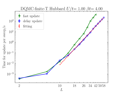
Figure 3: Comparison of the average time for update per sweep by local updates in DQMC-finite-T of the Hubbard model between fast update and delay update. Green line shows the cost of time with fast update. Blue line shows the cost of time with delay update. As the system size increases, the acceleration ratio of delay update relative to fast update becomes larger. The red dashed line denotes a rough fitting of the computation complexity of delay-update, it is around 6 as expected. If we perform simulate fitting for the blue line, the slope is a bit larger, but still around 6. We think the little deviation from 6 is finite size effect. This is also observed in Figs. 4, 6 and 7.

Before testing delay update, we first show why to optimize fast update part is important. We estimate the computation time proportions of various processes in a complete DQMC calculation. To control variables, we set Hubbard repulsive interaction $U/t=1$, the inverse temperature $\beta t=4$, and the time slice for Trotter decomposition $\Delta_{\tau}t=0.1$ uniformly.

For DQMC simulation, it mainly contains four parts, propagating, update, stabilization and measurement. The details of those parts can be found in Appendix A. Among them, update and stabilization have the complexity $\mathcal{O}(\beta N^{3})$ for DQMC-finite-T and $\mathcal{O}(\beta NN_{\text{p}}^{2})$ for DQMC-zero-T. The complexity of propagating part depends on the specific scheme used. For DQMC-finite-T, it has the complexity of $\mathcal{O}(\beta N^{3})$ if matrix product is used; $\mathcal{O}(\beta N^{2})$ if trotter decomposition is used for hopping part; $\mathcal{O}(\beta N^{2}\ln N)$ if FFT can be used for the hopping part. For DQMC-zero-T, the complexity for above three propagating schemes is $\mathcal{O}(\beta N^{2}N_{\text{p}})$, $\mathcal{O}(\beta NN_{\text{p}})$ and $\mathcal{O}(\beta NN_{\text{p}}\ln N)$, respectively. In our test, we use the second propagating scheme. The complexity of measurement part depends on the physical quantities people want to calculate. If we only consider equal-time measurement, this part typically has a smaller complexity, so we omit this part in our analysis. We also want to add a note that the unequal-time correlations can be got by propagating of equal-time correlations. Based on our test, propagating is not a bottleneck as long as we use the second or third propagating scheme which has a smaller complexity than update and stabilization.

For each simulation, we run 16 Markov chains, while each Markov chain contains 100 sweeps (divided into 5 bins). To further improve the estimation of computation time, we repeat the simulation for 5 times and calculate the average time. This setup applies to all the following estimations of computation time. When the system has a size of $42\times 42$, as shown in Fig. 2, whether it is DQMC-finite-T or DQMC-zero-T, the proportion of time taken by fast update to the total computation time exceeds 85$\%$. This indicates that optimizing local updates is highly essential for accelerating the DQMC.

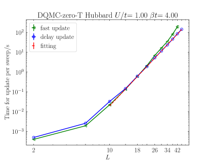
Figure 4: Comparison of the average time for update per sweep by local updates in DQMC-zero-T of the Hubbard model between fast update and delay update. Green line shows the cost of time with fast update. Blue line shows the cost of time with delay update. As the system size increases, the computation time of delay update becomes less than that of fast update.

Upon realizing this, we now compare the efficiency of fast update and delay update. We first consider finite-T calculation. We perform DQMC calculations on the Hubbard model with completely identical parameters on systems of different sizes, and we record the average computation time for update per sweep for each system size with different local update algorithm to make a comparison. The huge improvement is shown in Fig. 3. For the same system size, the computation time of delay update is less than that of fast update. Moreover, with an increase in system size, the acceleration factor of delay update continues to grow. When the system size reaches $42\times 42$, an acceleration of over tenfold has been achieved. Considering that the proportion of time taken by fast update to the total computation time has exceeded $85\%$, the overall speedup is about sevenfold. This allows us to elevate the computable system size from $42\times 42$ to $58\times 58$ while keeping the time cost nearly the same.

After that, we use the same conditions as above to compare delay update with fast update in DQMC-zero-T. Just as we discussed earlier, the computation complexity of fast update in DQMC-zero-T is lower $(\mathcal{O}(\beta NN_{p}^{2})<\mathcal{O}(\beta N^{3}))$, while delay update in DQMC-zero-T requires to calculate Green’s functions before and after each update. This makes the computation time of delay update in DQMC-zero-T longer compared to that in DQMC-finite-T. Consequently, for small system sizes, the computation time of delay update in DQMC-zero-T is longer than that of fast update. However, as the system size gradually increases, the demand for cache access also grows. In this scenario, delay update optimized for cache access show acceleration, and as the computational size expands, the acceleration factor also increases. With nearly the same time, delay updates can perform simulation on a system size of $46\times 46$, whereas fast updates can only handle a system size of $42\times 42$, as shown in Fig. 4.

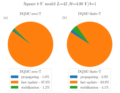
Figure 5: The proportion of total computation time cost by each process in a DQMC calculation of the spinless $t$-$V$ model on square lattice has a system size of $42\times 42$, with $\beta t=4$ and $V/t=1$ . (a) The proportion of each process in DQMC-zero-T. (b) The proportion of each process in DQMC-finite-T. The blue zone is propagation of the Green’s function, the orange zone is local updates and the green zone is numerical stabilization.

We have shown the superiors of delay update for onsite interaction. Now we show the speedup for extended interaction. We consider a case when $\Delta$ contains only two non-zero diagonal elements $(k=2)$. Let us consider $t$-$V$ model, which is a spinless fermion model with nearest-neighbor (NN) interaction. We consider it on a square lattice and the Hamiltonian is

$$H_{tV}=-t\sum_{\langle i,j\rangle}(c_{i}^{\dagger}c_{j}+\text{H.c.})+{V}\sum_{\langle i,j\rangle}(n_{i}-\frac{1}{2})(n_{j}-\frac{1}{2})$$ (29)

where $c_{i}^{\dagger}$ creates a fermion on site $i$, $t$ is the nearest-neighbour (NN) hopping term, and $V>0$ is the density repulsive interaction between NN sites. We also set $t=1$ as unit of energy and focus on half-filling case, and we also can use a suitable HS transformation to avoid sign problem[35, 36]. However, this transformation leads to two non-zero off-diagonal elements in $\Delta$ during updates. In order to employ delay updates, we require $\Delta$ to have only non-zero diagonal elements. To achieve this, we diagonalize $e^{V(\bm{s}_{i,l})}$, and propagating Green’s function to the representation where $\Delta$ is diagonal and has only two non-zero diagonal elements. In the spinless $t$-$V$ model, we set $V/t=1$, and all other conditions remain the same as the Hubbard model above. Due to the presence of two non-zero diagonal elements $(k=2)$, the computation time for local updates using fast updates is nearly four times longer than the Hubbard model. As a result, the vast majority of computation time is spent on local updates, as shown in Fig. 5.

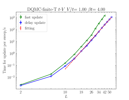
Figure 6: Comparison of the average time for update per sweep by local updates in DQMC-finite-T of the spinless t-V model between fast update and delay update. Green line shows the cost of time with fast update. Blue line shows the cost of time with delay update. The time curve exhibits behavior similar to that of the Hubbard model.

We also employed fast update and delay update separately to perform DQMC-finite-T calculations on the spinless $t$-$V$ model. After that we did the same comparison. With an increase in system size, the acceleration factor of delay update continues to grow. When the system size reaches $42\times 42$, an acceleration of over seven times in update part has been achieved. This allows us to elevate the computable system size from $42\times 42$ to $54\times 54$ while keeping the total time cost nearly the same.

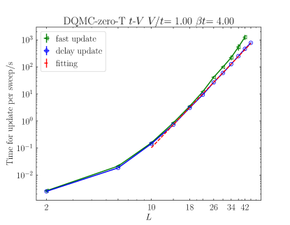
Figure 7: Comparison of the average time for update per sweep by local updates in DQMC-zero-T of the spinless t-V model between fast update and delay update. Green line shows the cost of time with fast update. Blue line shows the cost of time with delay update. Again, delay update shows superior performance than fast update for larger system size.

We also tested the acceleration of local updates in DQMC-zero-T using delay update in the same manner. It also demonstrates behavior similar to that of the DQMC-zero-T for the Hubbard model. Delay update still exhibits superior performance to fast update, when increasing the system size, the acceleration factor of delay update continues to grow. Furthermore, within nearly the same time frame, the system size for local updates can be increased from $42\times 42$ (fast update) to $46\times 46$ (delay update), as shown in Fig. 7.

IV Conclusion and discussion

In this work, we develop a generalized delay update scheme to accelerate DQMC simulation. It shows significant speedup for update both for onsite interaction and extended interaction. Based on our test, delay update can significantly enhance the efficiency of local updates. Moreover, as the system size increases, the computation acceleration factor of delay update continues to grow. By conducting tests on both DQMC-finite-T and DQMC-zero-T, we have found that delay update is particularly well-suited for DQMC-finite-T calculations. Moving forward, our future work involves further optimizing delay update especially for DQMC-zero-T. We aim to harness the algorithm’s potential within the DQMC-zero-T framework to achieve even better performance. An instructive way is to consider sub-matrix algorithm [54] to reduce the overhead of delay update [60]. We believe that the use of delay update can enable DQMC to simulate larger system sizes, thus allows for improved extrapolation of computational results to the thermodynamic limit, leading to more accurate phase diagrams and phase transitions.

Appendix A Outline of DQMC

A typical DQMC calculation is mainly composed of four parts, propagating, update, stabilization and measurement. In the following, we give some basic introduction. More details can be found in Refs. [16, 17, 18, 19, 20, 21, 22, 23, 24].

A.1 Propagating

When we have done all the sampling of auxiliary fields at a certain time $\tau_{1}$, we need to transform the equal-time Green’s function to the next time $\tau_{2}$, where $|\tau_{2}-\tau_{1}|=\Delta_{\tau}$. According to the definition of the equal-time Green’s function and the time evolution matrix $B$, we can easily get

$$G(\tau_{2},\tau_{2}) =B_{\bm{s}}(\tau_{2},\tau_{1})G(\tau_{1},\tau_{1})B_{\bm{s}}^{-1}(\tau_{2},\tau_{1})\ \ \text{for}\ \tau_{2}>\tau_{1}$$ (30)

$$G(\tau_{2},\tau_{2}) =B_{\bm{s}}(\tau_{1},\tau_{2})^{-1}G(\tau_{1},\tau_{1})B_{\bm{s}}(\tau_{1,}\tau_{2})\ \ \text{for}\ \tau_{2}<\tau_{1}$$ (31)

The process of calculating the equal-time Green’s function at different time with the time evolution matrix is called propagating. As mentioned in the main text, there are three methods to do propagating: matrix product, FFT and trotter decomposition. In the first way, we need to do the matrix product between time evolution $B$ matrices and $G(\tau_{1},\tau_{1})$, both of them are matrices of $N\times N$, so we need the computational complexity of $\mathcal{O}(N^{3})$ when do propagating across one time slice. A whole sweep requires going through $\mathcal{O}(\beta)$ numbers of time slices, therefore, the computational complexity is $\mathcal{O}(\beta N^{3})$. If the system has lattice translation symmetry, we can use FFT to reduce the computational complexity. For example, to calculate $e^{-\Delta_{\tau}K}G(\tau_{1},\tau_{1})$, we can perform FFT on the row index of $G(\tau_{1},\tau_{1})$, reducing the computational complexity from $\mathcal{O}(N^{2})$ to $\mathcal{O}(N\ln N)$ for getting each column of the resulting matrix. We need to perform $N$ times of FFT to get all columns of the resulting matrix, so that using FFT to do the propagating for $\mathcal{O}(\beta)$ numbers of time slices reduces the complexity to $\mathcal{O}(\beta N^{2}\ln N)$. In the end, we consider the propagating using the trotter decomposition. For example, $B_{\bm{s}}(\tau_{2},\tau_{1})G(\tau_{1},\tau_{1})=e^{V(\bm{s})}e^{-\Delta_{\tau}K}G(\tau_{1},\tau_{1})$, where $e^{-\Delta_{\tau}K}G(\tau_{1},\tau_{1})$ can be trotter decomposed into $e^{-\Delta_{\tau}K}\approx\prod_{b}e^{-\Delta_{\tau}K_{b}}$, where each $e^{-\Delta_{\tau}K_{b}}$ is a sparse matrix with the non-zero elements $(e^{-\Delta_{\tau}K_{b}})_{ij}$ ($i$ and $j$ belongs to the two sites of the hopping bond $b$). The computational complexity of the calculation of a certain bond of $e^{-\Delta_{\tau}K_{b}}G(\tau_{1},\tau_{1})$ is $\mathcal{O}(N)$, so the computational complexity of propagating using trotter decomposition involves $\mathcal{O}(\beta N)$ numbers of bonds, leading to the computation complexity of $\mathcal{O}(\beta N^{2})$. Similarly, multiply $e^{V(\bm{s})}$ to the left side of $e^{-\Delta_{\tau}K_{b}}G(\tau_{1},\tau_{1})$ can also be done using trotter decomposition, and it also has the same computational complexity $\mathcal{O}(\beta N^{2})$ for a whole sweep.

Having discussed the propagating in the DQMC-finite-T, now we turn to the DQMC-zero-T. The propagating in the DQMC-zero-T is similar as which in the DQMC-finite-T. The only difference between them is the time evolution matrix $B$ applies on $B_{\bm{s}}^{\rangle}(\tau_{1})$ or $B_{\bm{s}}^{\langle}(\tau_{1})$, which is a matrix of $N\times N_{p}$ or $N_{p}\times N$. Take $B_{\bm{s}}(\tau_{2},\tau_{1})B^{\rangle}_{\bm{s}}(\tau_{1})$ as an example, the computational complexity of a certain column is the same, however, there is only $N_{p}$ columns, so the computational complexity of the propagating with matrix product, FFT and trotter decomposition is $O(\beta N^{2}N_{p})$, $O(\beta N_{p}N\ln N)$ and $O(\beta N_{p}N)$ respectively.

A.2 Update

In the QMC simulation, we need to loop over all the configurations and meet the demand of the detailed balance condition when accepting them, which is called update. In the DQMC, we convert the electron interaction term into the coupling term between the auxiliary field and the fermions, therefore, the sampling process of DQMC can be converted into the following steps: select a fermion lattice point and flip the auxiliary field on the lattice point one by one, then we need to determine whether to accept this auxiliary field configuration through calculating the weight and the equal-time Green’s function. If the proposed flip of the auxiliary field is accepted, we need to update the equal-time Green’s function. Usually, we use the fast update scheme. In this article, we proposed a general delay update scheme, which can greatly improve the efficiency of update compared to fast update. The details of fast update and delay update are discussed in Sec. II.

A.3 Stabilization

In the process of the update, the equal-time Green’s function plays a central role. Since each update of the Green’s function is a cumulative update based on the original Green’s function and needs to be propagated for many times, the accumulation of numerical errors will become larger and larger. In order to reduce numerical errors, we need to recalculate the equal-time Green’s function with the time evolution matrix $B$ at the set intervals. Therefore, the key part is how to obtain the $B$ matrix through stable matrix multiplication. $B$ is a series of matrix multiplications and people usually use the SVD or QR decomposition to stabilize the numerical value of $B$ in the multiplication process [61, 24], which is called stabilization. For example, we have

$$B_{\mathbf{s}}(n\tau_{s},0)=\mathbf{U}_{n}\underbrace{\left[\begin{array}[]{cccc}\text{\Large X}&&&\\ &\text{\large X}&&\\ &&\text{\small X}&\\ &&&\text{\tiny X}\\ \end{array}\right]}_{{\mathbf{D}_{n}}}\mathbf{V}_{n}$$ (32)

and we can perform singular value decomposition every $\tau_{s}$ step

$$B_{\bm{s}}((n+1)\tau_{s},0) =B_{\bm{s}}((n+1)\tau_{s},n\tau_{s})\mathbf{U}_{n}\underbrace{\left[\begin{array}[]{cccc}\text{\Large X}&&&\\ &\text{\large X}&&\\ &&\text{\small X}&\\ &&&\text{\tiny X}\\ \end{array}\right]}_{{\mathbf{D}_{n}}}\mathbf{V}_{n}$$ (33)

$$=\underbrace{\left[\begin{array}[]{cccc}\text{\Large X}&\text{\large X}&\text{\small X}&\text{\tiny X}\\ \text{\Large X}&\text{\large X}&\text{\small X}&\text{\tiny X}\\ \text{\Large X}&\text{\large X}&\text{\small X}&\text{\tiny X}\\ \text{\Large X}&\text{\large X}&\text{\small X}&\text{\tiny X}\\ \end{array}\right]}_{{B_{\bm{s}}((n+1)\tau_{s},n\tau_{s})\mathbf{U}_{n}\mathbf{D}_{n}}}\mathbf{V}_{n}$$

$$=\mathbf{U}_{n+1}\underbrace{\left[\begin{array}[]{cccc}\text{\Large X}&&&\\ &\text{\large X}&&\\ &&\text{\small X}&\\ &&&\text{\tiny X}\\ \end{array}\right]}_{{\mathbf{D}_{n+1}}}\underbrace{\mathbf{V}^{\prime}\mathbf{V}_{n}}_{{\mathbf{V}_{n+1}}}$$

$$=\mathbf{U}_{n+1}\mathbf{D}_{n+1}\mathbf{V}_{n+1}$$

Correspondingly, for $B_{\bm{s}}(\beta,n\tau_{s})$, We also make a similar decomposition, The above $\mathbf{U}_{n}$, $\mathbf{D}_{n}$, and $\mathbf{V}_{n}$ matrices all need to be stored. At imaginary time $\tau=n\tau_{s}$, we recalculate the equal-time Green’s function. From the above decomposition, we have $B_{\bm{s}}(\tau,0)=\mathbf{U}_{R}\mathbf{D}_{R}\mathbf{V}_{R}$ and $B_{\bm{s}}(\beta,\tau)=\mathbf{V}_{L}\mathbf{D}_{L}\mathbf{U}_{L}$, the equal-time Green’s function is

$$G\left(n\tau_{s},n\tau_{s}\right)= {[\mathbf{1}+B_{\bm{s}}(\tau,0)B_{\bm{s}}(\beta,\tau)]^{-1}}$$ (34)

$$= {\left[\mathbf{1}+\mathbf{U}_{R}\mathbf{D}_{R}\mathbf{V}_{R}\mathbf{V}_{L}\mathbf{D}_{L}\mathbf{U}_{L}\right]^{-1}}$$

$$= \mathbf{U}_{L}^{-1}\left[\left(\mathbf{U}_{L}\mathbf{U}_{R}\right)^{-1}+\mathbf{D}_{R}\left(\mathbf{V}_{R}\mathbf{V}_{L}\right)\mathbf{D}_{L}\right]^{-1}\mathbf{U}_{R}^{-1}$$

$$= \mathbf{U}_{L}^{-1}\left[\left(\mathbf{U}_{L}\mathbf{U}_{R}\right)^{-1}+\mathbf{D}_{R}^{\max}\mathbf{D}_{R}^{\min}\left(\mathbf{V}_{R}\mathbf{V}_{L}\right)\mathbf{D}_{L}^{\min}\mathbf{D}_{L}^{\max}\right]^{-1}\mathbf{U}_{R}^{-1}$$

$$= \mathbf{U}_{L}^{-1}\left(\mathbf{D}_{L}^{\max}\right)^{-1}\left[\left(\mathbf{D}_{R}^{\max}\right)^{-1}\left(\mathbf{U}_{L}\mathbf{U}_{R}\right)^{-1}\left(\mathbf{D}_{L}^{\max}\right)^{-1}\right.$$

$$\left.+\mathbf{D}_{R}^{\min}\mathbf{V}_{R}\mathbf{V}_{L}\mathbf{D}_{L}^{\min}\right]^{-1}\left(\mathbf{D}_{R}^{\max}\right)^{-1}\mathbf{U}_{R}^{-1}$$

where $\mathbf{D}_{R}^{\min}(i,i)=\min\{\mathbf{D}_{R}(i,i),1\}$ and $\mathbf{D}_{R}^{\max}(i,i)=\max\{\mathbf{D}_{R}(i,i),1\}$. Generally speaking, the selection of the interval for numerical stability $\tau_{s}$ is related to the severity of numerical instability. It is generally required that the selection of $\tau_{s}$ should make the numerical error of the equal-time Green’s function below $10^{-6}$.

In the end, we discuss the computational complexity of stabilization briefly. At each time when we do the stabilization we need to calculate the equal-time Green’s function with $\mathbf{U}_{R}$, $\mathbf{D}_{R}$, $\mathbf{V}_{R}$, $\mathbf{V}_{L}$, $\mathbf{D}_{L}$ and $\mathbf{U}_{L}$, the computational complexity of each stabilization is $\mathcal{O}(N^{3})$ and we do the stabilization with an interval of $\tau_{s}$ time slices, therefore we need do the stabilization $\mathcal{O}(\frac{\beta}{\tau_{s}})$ times during a sweep. As usually $\tau_{s}$ is a fixed value, the total computational complexity for stabilization is $\mathcal{O}(\beta N^{3})$

A.4 Measurement

In the end, We use Wick’s theorem and the Green’s function to perform the measurement. The equal-time Green’s function can be used to calculate the energy, order parameters and various equal-time correlation functions of the system. The unequal-time Green’s functions can be used to calculate dynamic properties of the system. The unequal-time Green’s functions are defined as

$$G_{ij}(\tau_{2},\tau_{1})\equiv\langle c_{i}(\tau_{2})c_{j}^{\dagger}(\tau_{1})\rangle$$ (35)

$$G_{ij}(\tau_{1},\tau_{2})\equiv-\langle c_{j}^{\dagger}(\tau_{2})c_{i}(\tau_{1})\rangle$$ (36)

where $\tau_{2}\geq\tau_{1}$. We can get the unequal-time Green’s function in the presentation of the time evolution matrix and the equal-time Green’s function as below

$$G(\tau_{2},\tau_{1}) =B_{\bm{s}}(\tau_{2},\tau_{1})G(\tau_{1},\tau_{1})$$ (37)

$$G(\tau_{1},\tau_{2}) =-B^{-1}_{\bm{s}}(\tau_{2},\tau_{1})\left[I-G(\tau_{2},\tau_{2})\right]$$ (38)

then we can use the Wick’s theorem to get dynamic correlations of the system. We take the spin correlation as an example. For convenience, we define a hermitian conjugation of the equal-time Green’s function

$$G^{c}_{ij}(\tau,\tau)\equiv\langle c_{i}^{\dagger}(\tau)c_{j}(\tau)\rangle$$ (39)

With the help of spin $SU(2)$ symmetry, the spin correlation function can be written as

$$\langle\mathbf{S}_{i}\cdot\mathbf{S}_{j}\rangle =\frac{3}{2}\langle S^{+}_{i}S^{-}_{j}\rangle$$ (40)

$$=\frac{3}{2}\langle c^{\dagger}_{i\uparrow}c_{i\downarrow}c^{\dagger}_{j\downarrow}c_{j\uparrow}\rangle$$

$$=\frac{3}{2}\langle c^{\dagger}_{i\uparrow}c_{j\uparrow}\rangle\langle c_{i\downarrow}c^{\dagger}_{j\downarrow}\rangle$$

$$=\frac{3}{2}G^{c}_{ij}G_{ij}$$

In the same way, we can get the dynamical spin correlation function as $\langle S^{+}_{i}(\tau)S^{-}_{j}(0)\rangle=-G_{ji}(0,\tau)G_{ij}(\tau,0)$.

We use trotter decomposition to calculate the unequal-time Green’s function (Eq.(37,38)), similar to the case of using trotter decomposition in the propagating part, the computational complexity is $O(\beta N^{2})$ for the DQMC-finite-T and $O(\beta N_{p}N)$ for the DQMC-zero-T.

References

- Bednorz and Müller [1986] J. G. Bednorz and K. A. Müller, Zeitschrift für Physik B Condensed Matter 64, 189 (1986).
- Bednorz and Müller [1988] J. G. Bednorz and K. A. Müller, Rev. Mod. Phys. 60, 585 (1988).
- Johnston [2010] D. C. Johnston, Advances in Physics 59, 803 (2010).
- Lee et al. [2006] P. A. Lee, N. Nagaosa, and X.-G. Wen, Rev. Mod. Phys. 78, 17 (2006).
- Sun et al. [2023] H. Sun, M. Huo, X. Hu, J. Li, Z. Liu, Y. Han, L. Tang, Z. Mao, P. Yang, B. Wang, et al., Nature , 1 (2023).
- Tsui et al. [1982] D. C. Tsui, H. L. Stormer, and A. C. Gossard, Phys. Rev. Lett. 48, 1559 (1982).
- Moore and Read [1991] G. Moore and N. Read, Nuclear Physics B 360, 362 (1991).
- Stormer et al. [1999] H. L. Stormer, D. C. Tsui, and A. C. Gossard, Rev. Mod. Phys. 71, S298 (1999).
- Hansson et al. [2017] T. H. Hansson, M. Hermanns, S. H. Simon, and S. F. Viefers, Rev. Mod. Phys. 89, 025005 (2017).
- Anderson [1973] P. Anderson, Materials Research Bulletin 8, 153 (1973).
- Kitaev [2006] A. Kitaev, Annals of Physics 321, 2 (2006).
- Balents [2010] L. Balents, Nature 464, 199 (2010).
- Zhou et al. [2017] Y. Zhou, K. Kanoda, and T.-K. Ng, Reviews of Modern Physics 89, 025003 (2017).
- Broholm et al. [2020] C. Broholm, R. Cava, S. Kivelson, D. Nocera, M. Norman, and T. Senthil, Science 367, eaay0668 (2020).
- Savary and Balents [2017] L. Savary and L. Balents, Reports on Progress in Physics 80, 016502 (2017).
- Blankenbecler et al. [1981] R. Blankenbecler, D. J. Scalapino, and R. L. Sugar, Phys. Rev. D 24, 2278 (1981).
- Scalapino and Sugar [1981] D. J. Scalapino and R. L. Sugar, Phys. Rev. B 24, 4295 (1981).
- Hirsch [1983] J. E. Hirsch, Phys. Rev. B 28, 4059 (1983).
- Sugiyama and Koonin [1986] G. Sugiyama and S. Koonin, Annals of Physics 168, 1 (1986).
- Sorella et al. [1988] S. Sorella, E. Tosatti, S. Baroni, R. Car, and M. Parrinello, International Journal of Modern Physics B 02, 993 (1988).
- Sorella et al. [1989] S. Sorella, S. Baroni, R. Car, and M. Parrinello, Europhysics Letters (EPL) 8, 663 (1989).
- Loh Jr and Gubernatis [1992] E. Loh Jr and J. Gubernatis, Electronic Phase Transitions 32, 177 (1992).
- Koonin et al. [1997] S. E. Koonin, D. J. Dean, and K. Langanke, Physics reports 278, 1 (1997).
- Assaad and Evertz [2008] F. Assaad and H. Evertz, World-line and determinantal quantum monte carlo methods for spins, phonons and electrons, in Computational Many-Particle Physics, edited by H. Fehske, R. Schneider, and A. Weiße (Springer Berlin Heidelberg, Berlin, Heidelberg, 2008) pp. 277–356.
- Hirsch [1985] J. E. Hirsch, Phys. Rev. B 31, 4403 (1985).
- White et al. [1989] S. R. White, D. J. Scalapino, R. L. Sugar, E. Y. Loh, J. E. Gubernatis, and R. T. Scalettar, Phys. Rev. B 40, 506 (1989).
- Assaad [1999] F. F. Assaad, Phys. Rev. Lett. 83, 796 (1999).
- Scalapino [2007] D. Scalapino, Numerical studies of the 2d hubbard model, in Handbook of High-Temperature Superconductivity (Springer, 2007) pp. 495–526.
- Zheng et al. [2011] D. Zheng, G.-M. Zhang, and C. Wu, Phys. Rev. B 84, 205121 (2011).
- Hohenadler et al. [2011] M. Hohenadler, T. C. Lang, and F. F. Assaad, Phys. Rev. Lett. 106, 100403 (2011).
- Berg et al. [2012] E. Berg, M. A. Metlitski, and S. Sachdev, Science 338, 1606 (2012).
- Hohenadler and Assaad [2013] M. Hohenadler and F. F. Assaad, Journal of Physics: Condensed Matter 25, 143201 (2013).
- Assaad and Herbut [2013] F. F. Assaad and I. F. Herbut, Phys. Rev. X 3, 031010 (2013).
- LeBlanc et al. [2015] J. P. F. LeBlanc, A. E. Antipov, F. Becca, I. W. Bulik, G. K.-L. Chan, C.-M. Chung, Y. Deng, M. Ferrero, T. M. Henderson, C. A. Jiménez-Hoyos, E. Kozik, X.-W. Liu, A. J. Millis, N. V. Prokof’ev, M. Qin, G. E. Scuseria, H. Shi, B. V. Svistunov, L. F. Tocchio, I. S. Tupitsyn, S. R. White, S. Zhang, B.-X. Zheng, Z. Zhu, and E. Gull (Simons Collaboration on the Many-Electron Problem), Phys. Rev. X 5, 041041 (2015).
- Li et al. [2015] Z.-X. Li, Y.-F. Jiang, and H. Yao, Phys. Rev. B 91, 241117 (2015).
- Wang et al. [2015] L. Wang, Y.-H. Liu, M. Iazzi, M. Troyer, and G. Harcos, Phys. Rev. Lett. 115, 250601 (2015).
- He et al. [2016] Y.-Y. He, H.-Q. Wu, Y.-Z. You, C. Xu, Z. Y. Meng, and Z.-Y. Lu, Phys. Rev. B 93, 115150 (2016).
- Otsuka et al. [2016] Y. Otsuka, S. Yunoki, and S. Sorella, Phys. Rev. X 6, 011029 (2016).
- Assaad and Grover [2016] F. Assaad and T. Grover, Physical Review X 6, 041049 (2016).
- Zhou et al. [2016] Z. Zhou, D. Wang, Z. Y. Meng, Y. Wang, and C. Wu, Phys. Rev. B 93, 245157 (2016).
- Gazit et al. [2017] S. Gazit, M. Randeria, and A. Vishwanath, Nature Physics 13, 484 (2017).
- Berg et al. [2019] E. Berg, S. Lederer, Y. Schattner, and S. Trebst, Annual Review of Condensed Matter Physics 10, 63 (2019).
- Li and Yao [2019] Z.-X. Li and H. Yao, Annual Review of Condensed Matter Physics 10, 337 (2019).
- Xu et al. [2019a] X. Y. Xu, Z. H. Liu, G. Pan, Y. Qi, K. Sun, and Z. Y. Meng, Journal of Physics: Condensed Matter 31, 463001 (2019a).
- Liu et al. [2019] Y. Liu, Z. Wang, T. Sato, M. Hohenadler, C. Wang, W. Guo, and F. F. Assaad, Nature Communications 10, 2658 (2019).
- Xu et al. [2019b] X. Y. Xu, Y. Qi, L. Zhang, F. F. Assaad, C. Xu, and Z. Y. Meng, Physical Review X 9, 021022 (2019b).
- Chen et al. [2019] C. Chen, X. Y. Xu, Z. Y. Meng, and M. Hohenadler, Phys. Rev. Lett. 122, 077601 (2019).
- Zhang et al. [2019] Y.-X. Zhang, W.-T. Chiu, N. C. Costa, G. G. Batrouni, and R. T. Scalettar, Phys. Rev. Lett. 122, 077602 (2019).
- Xu and Grover [2021] X. Y. Xu and T. Grover, Phys. Rev. Lett. 126, 217002 (2021).
- Zhang et al. [2021] X. Zhang, G. Pan, Y. Zhang, J. Kang, and Z. Y. Meng, Chinese Physics Letters 38, 077305 (2021).
- Hofmann et al. [2022] J. S. Hofmann, E. Khalaf, A. Vishwanath, E. Berg, and J. Y. Lee, Physical Review X 12, 011061 (2022).
- Mondaini et al. [2022] R. Mondaini, S. Tarat, and R. T. Scalettar, Science 375, 418 (2022).
- Alvarez et al. [2008] G. Alvarez, M. S. Summers, D. E. Maxwell, M. Eisenbach, J. S. Meredith, J. M. Larkin, J. Levesque, T. A. Maier, P. R. Kent, E. F. D’Azevedo, et al., in SC’08: Proceedings of the 2008 ACM/IEEE Conference on Supercomputing (IEEE, 2008) pp. 1–10.
- Nukala et al. [2009] P. K. V. V. Nukala, T. A. Maier, M. S. Summers, G. Alvarez, and T. C. Schulthess, Phys. Rev. B 80, 195111 (2009).
- Gull et al. [2011] E. Gull, P. Staar, S. Fuchs, P. Nukala, M. S. Summers, T. Pruschke, T. C. Schulthess, and T. Maier, Phys. Rev. B 83, 075122 (2011).
- Gutzwiller [1963] M. C. Gutzwiller, Phys. Rev. Lett. 10, 159 (1963).
- Hubbard [1963] J. Hubbard, Proceedings of the Royal Society of London. Series A. Mathematical and Physical Sciences 276, 238 (1963).
- Arovas et al. [2022] D. P. Arovas, E. Berg, S. A. Kivelson, and S. Raghu, Annual review of condensed matter physics 13, 239 (2022).
- Qin et al. [2022] M. Qin, T. Schäfer, S. Andergassen, P. Corboz, and E. Gull, Annual Review of Condensed Matter Physics 13, 275 (2022).
- [60] F. Sun and X. Y. Xu, in prepareration. .
- Loh et al. [2005] E. Loh, J. Gubernatis, R. Scalettar, S. White, D. Scalapino, and R. Sugar, International Journal of Modern Physics C 16, 1319 (2005).