Relational Concept Based Models

Relational Concept Based Models

Abstract

The design of interpretable deep learning models working in relational domains poses an open challenge: interpretable deep learning methods, such as Concept-Based Models (CBMs), are not designed to solve relational problems, while relational models are not as interpretable as CBMs. To address this problem, we propose Relational Concept-Based Models, a family of relational deep learning methods providing interpretable task predictions. Our experiments, ranging from image classification to link prediction in knowledge graphs, show that relational CBMs (i) match generalization performance of existing relational black-boxes (as opposed to non-relational CBMs), (ii) support the generation of quantified concept-based explanations, (iii) effectively respond to test-time interventions, and (iv) withstand demanding settings including out-of-distribution scenarios, limited training data regimes, and scarce concept supervisions.

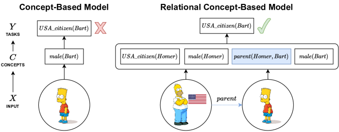
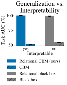
Figure 1: (left) Standard CBMs fail to predict Bart’s citizenship. (center) Relational CBMs can correctly predict and explain Bart’s citizenship by considering Homer’s citizenship and his status as Bart’s father (binary concept) [pics from https://www.pngall.com/the-simpsons-png/]. (right) Relational CBMs match the task generalization performance of equivalent relational black-boxes in the Tower of Hanoi dataset, as opposed to non-relational CBMs.

1 Introduction

Chemistry, politics, economics, traffic jams: we constantly rely on relations to describe, explain, and solve real-world problems. For instance, we can easily deduce Bart’s citizenship if we consider Homer’s citizenship and his status as Bart’s father (Fig. 1, center). While relational deep learning models (Scarselli et al. 2008; Micheli 2009; Wang et al. 2017; Manhaeve et al. 2018) can solve such problems effectively, the design of interpretable neural models capable of relational reasoning is still an open challenge.

Among deep learning methods, Concept-Based Models (CBMs, Fig. 1, left) (Koh et al. 2020) emerged as interpretable methods explaining their predictions by first mapping input features to a set of human-understandable concepts (e.g., “red”,“round”) and then using such concepts to solve given tasks (e.g., “apple”). However, existing CBMs are not well-suited for addressing relational problems as they can process only one input entity at a time by construction (Fig. 1, left; Sec. 3 for technical details). To solve relational problems, CBMs would need to handle concepts/tasks involving multiple entities (e.g., the concept “parent” which depends on both the entity “Homer” and “Bart”), thus forcing CBMs to process more entities at a time. While existing relational deep learning methods may solve such problems effectively (e.g., correctly predicting Bart’s citizenship), they are still unable to explain their predictions, as CBMs could do (e.g., Bart is a USA citizen because Homer is a USA citizen and Homer is the father of Bart). As a result, a knowledge gap persists in the existing literature: a deep learning model capable of relational reasoning (akin to a Graph Neural Network (Scarselli et al. 2008; Micheli 2009)), while also being interpretable (akin to a CBM).

To address this gap, we propose Relational Concept-Based Models (Relational CBMs, Sec. 4), a family of concept-based models where both concepts and tasks may depend on multiple entities. The results of our experiments (Sec. 5, 6) show that relational CBMs: (i) match the generalization performance of existing relational black-boxes (as opposed to standard CBMs, Fig. 1, right), (ii) support the generation of quantified concept-based explanations, (iii) effectively respond to test-time concept and rule interventions improving their task performance, (iv) withstand demanding test scenarios including out-of-distribution settings, limited training data regimes, and scarce concept supervisions.

2 Background

Concept-based models.

A concept-based model is a function composing: (i) a concept encoder $g:X\to C$ mapping each entity $e$ with feature representation $x_{e}\in X\subseteq\mathbb{R}^{d}$ (e.g., an image) to a set of $k$ concepts $c\in C\subseteq[0,1]^{k}$ (e.g., “red”,“round”), and (ii) a task predictor $f:C\to Y$ mapping concepts to a set of $m$ tasks $y\in Y\subseteq[0,1]^{m}$ (e.g., “apple”,“tomato”). Each component $g_{i}$ and $f_{j}$ denotes the truth-degree of the $i$-th concept and $j$-th task, respectively.

Relational languages.

A relational setting can be outlined using a function-free first-order logic language $\mathcal{L}=(\mathcal{X},\mathcal{V},\mathcal{P})$, where $\mathcal{X}$ is a finite set of constants for specific domain entities, $\mathcal{V}$ is a set of variables for anonymous entities, and $\mathcal{P}$ is a set of $n$-ary predicates for relations among entities. The central objects of a relational language are atoms, i.e. expressions $P(t_{1},\ldots,t_{n})$, where $P$ is an $n$-ary predicate and $t_{1},\ldots,t_{n}$ are constants or variables. In case $t_{1},\ldots,t_{n}$ are all constants, $P(t_{1},\ldots,t_{n})$ is called a ground atom. Examples of atoms can be $\textit{male}(\textit{Bart})$ and $\textit{larger}(u,v)$, with $Bart\in\mathcal{X}$ and $u,v\in\mathcal{V}$. Given a set of atoms $\Gamma$ defined on a joint set of variables $V=\{v_{1},\ldots,v_{n}\}$, grounding is the process of applying a substitution $\theta_{V}=\{v_{1}/x_{1},...,v_{n}/x_{n}\}$ to $\Gamma$, i.e. substituting all the variables $v_{i}$ with some constants $x_{i}$, according to $\theta_{V}$. For example, given $\Gamma=[\textit{parent}(v_{1},v_{2}),\textit{parent}(v_{2},v_{3})]$ and the substitution $\theta=\{v_{1}/\textit{Abe},v_{2}/\textit{Homer},v_{3}/\textit{Bart}\}$, we can obtain the ground list ${\theta}\Gamma=[\textit{parent}(\textit{Abe},\textit{Homer}),\textit{parent}(\textit{Homer},\textit{Bart})]$. Logic rules are defined as usual by using logic connectives $\{\neg,\wedge,\vee,\rightarrow\}$ and quantifiers $\{\forall,\exists\}$.

Figure 2: In Relational CBMs (i) the concept encoder $g$ maps input entities to a set of intermediate concepts (red/green indicate the ground atom label false/true), (ii) the relational template guides the selection of concept atoms by considering all the possible variable substitutions in $\Theta$, (iii) the task predictor $f$ maps the selected concept atoms into a task prediction, and (iv) the aggregator $\oplus$ combines all evidence into a final task prediction.

3 Concept-Based Model Templates

This work addresses two main research questions: can we define CBMs in relational settings?, and how do we instantiate relational CBMs? To start answering the first question, we can define (non-relational) CBMs in a relational language by (i) associating a constant in $\mathcal{X}$ for each element in $X$, (ii) using unary predicates in $\mathcal{P}=\{c_{1},\ldots,c_{k},y_{1},\ldots,y_{m}\}$ to represent concepts and tasks, and (iii) inferring the truth-degrees of ground atoms $c_{i}(x)$ and $y_{j}(x)$ using $g_{i}(x)$ and $f_{j}(g(x))$, for $x\in X$ and $i=1,\ldots,k$, $j=1,\ldots,m$, respectively. In a relational language, we can formalize that CBMs infer tasks as a function of concepts by introducing the notion of a CBM template.

Definition 3.1.

Given a task $y$ and the concepts $c_{1},\ldots,c_{k}$, we call a CBM template for $y$, the expression:

$$y(v)\mathop{:\!\!-}c_{1}(v),\ldots,c_{k}(v)\ .$$ (1)

Definition 3.1 specifies the input-output interface of a CBM. The variable $v$ is implicitly universally quantified, meaning that the template can be read as “for each substitution $x_{e}$ for $v$, the task $y$ on $x_{e}$ is a mapping of the concepts on $x_{e}$”. For example, given the unary predicates $\mathcal{P}=\{c_{\textit{red}},c_{\textit{round}},y_{\textit{tomato}}\}$, a possible CBM template is $y_{\textit{tomato}}(v)\mathop{:\!\!-}c_{\textit{red}}(v),c_{\textit{round}}(v)$.

In relational domains we need to generalize Eq. 1 as both tasks and concepts may refer to n-ary entity tuples $(x_{1},\ldots,x_{n})\in X^{n}$ e.g., $father(Homer,Bart)$. This raises the question: given a task atom, which concept atoms should go in a relational CBM template? The next paragraph discusses such question. Readers only interested in the proposed solution can skip to Sec. 4.

Naive relational CBM templates.

We discuss the design of relational CBM templates on a simplified, yet general, setting (the same argument holds when considering predicates of higher arity and multiple tasks). Consider a binary task $y$ and a list of concepts split into two disjoint lists of predicates, i.e. unary $c^{\prime}(v)=[c^{\prime}_{1}(v),\ldots,c^{\prime}_{k_{1}}(v)]$ and binary $c^{\prime\prime}(v_{1},v_{2})=[c^{\prime\prime}_{1}(v_{1},v_{2}),\ldots,c^{\prime\prime}_{k_{2}}(v_{1},v_{2})]$, respectively. In this setting, a naive CBM template may specify the task $y(v_{1},v_{2})$ using all the unary concepts on $v_{1}$ and $v_{2}$, and all the binary concepts on the pair $(v_{1},v_{2})$, i.e. $y(v_{1},v_{2})\mathop{:\!\!-}c^{\prime}(v_{1}),c^{\prime}(v_{2}),c^{\prime\prime}(v_{1},v_{2})$. However, this template only considers the ordered tuple $(v_{1},v_{2})$, thus preventing to model tasks which depend on permutations or repetitions of $v_{1},v_{2}$, e.g. $\textit{father}(\textit{Homer},\textit{Bart})$ can be inferred from $\textit{son}(\textit{Bart},\textit{Homer})$, but cannot be inferred from $\textit{son}(\textit{Homer},\textit{Bart})$. Hence, we may consider all the binary concepts defined on all the ordered tuples on $\{v_{1},v_{2}\}$ i.e.,

$$y(v_{1},v_{2})\mathop{:\!\!-}c^{\prime}(v_{1}),c^{\prime}(v_{2}),c^{\prime\prime}(v_{1},v_{1}),c^{\prime\prime}(v_{2},v_{2}),$$

$$c^{\prime\prime}(v_{1},v_{2}),c^{\prime\prime}(v_{2},v_{1})\ .$$ (2)

While this template handles multiple entities, it still overlooks relational dependencies among entities in different tuples. For instance, this template prevents to infer the task $\textit{grandparent}(\textit{Abe},\textit{Bart})$ using the concepts $\textit{parent}(\textit{Abe},\textit{Homer})$ and $\textit{parent}(\textit{Homer},\textit{Bart})$, as the task atom does not directly depend on the entity Homer. To handle connections through entities which do not explicitly appear in task atoms, we can add to the previous task template all the concepts grounded on all known entities:

$$y(v_{1},v_{2})\mathop{:\!\!-}c^{\prime}(v_{1}),c^{\prime}(v_{2}),c^{\prime}(x_{1}),c^{\prime}(x_{2}),c^{\prime}(x_{3}),\ldots,$$

$$c^{\prime\prime}(v_{1},v_{1}),c^{\prime\prime}(v_{1},v_{2}),c^{\prime\prime}(v_{1},x_{1}),c^{\prime\prime}(v_{1},x_{2}),\ldots,$$

$$c^{\prime\prime}(v_{2},v_{1}),c^{\prime\prime}(v_{2},v_{2}),c^{\prime\prime}(v_{2},x_{1}),c^{\prime\prime}(v_{2},x_{2}),\ldots,$$

$$c^{\prime\prime}(x_{1},v_{1}),c^{\prime\prime}(x_{1},v_{2}),c^{\prime\prime}(x_{1},x_{1}),c^{\prime\prime}(x_{1},x_{2}),\ldots$$ (3)

However, the scalability of this choice would be restricted to tasks involving a handful of entities, as a CBM would need to consider everything we could possibly know about the entire world. As a result, each sample would contain an entire “flat” world, without being able to exploit any underlying relational substructure. Even worse, this hinders the generalization capabilities of the model: even a small modification to the world like, the introduction of just one new entity, would require either to define and train a new model from scratch, or to ignore the new entity altogether. For instance, once a new entity Lisa is introduced (literally Lisa comes to the world), $\textit{hasUniqueSon}(\textit{Homer},\textit{Bart})$ would become false knowing e.g., that $\textit{parent}(\textit{Homer},\textit{Lisa})$ is true, but the template in Eq. 3 would not allow to consider Lisa at all.

4 Relational Concept-Based Models

A Relational Concept-based Model is a function combining a concept encoder $g$ and a task predictor $f$, where both concepts and tasks may depend on multiple entities. To describe relational CBMs, we illustrate their architectures (Sec. 4.1), the learning problem they can solve (Sec. 4.2) and a set of concrete relational CBMs (Sec. 4.3).

4.1 Relational Concept-Based Architectures

The three key differences turning CBMs into relational CBMs are: (i) the concept encoder $g$ maps tuples of entities into concept scores, (ii) the input-output interface of the task predictor $f$ depends on the structure of a relational template (see Eq. 4, generalizing Eq. 1), and (iii) the final task predictions are obtained by aggregating the predictions of $f$ over all groundings of the template (Eq. 5).

Relational concept encoder.

In relational CBMs, each concept may depend on multiple entities $\bar{x}=(x_{1},\ldots,x_{n})$. This prompts the concept encoder to process input features from entities $\bar{x}$ and generate the corresponding concept activation. Formally, for each $n$-ary concept, the relational concept encoder $g_{i}(\bar{x})$ (where $g_{i}:X^{n}\to[0,1]$, for $i=1,\ldots,k$) predicts concept predicates $c_{i}(\bar{x})$.

Relational CBM template.

In relational CBMs, the input configuration of the task predictor $f$ depends on a relational CBM template. This relational template generalizes the one in Eq. (1), as it includes in concept atoms a fixed number of extra variables representing entities which do not explicitly appear in task atoms. More specifically, we define the template of a relational CBM as a width-customizable mapping whose expressivity may span from Eq. (2) to Eq. (3).

Definition 4.1.

Given an $n$-ary task $y$, the concepts $c_{1},\ldots,c_{k}$, and an integer $w\geq 0$, we define a relational CBM template of width $w$ as the expression:

$$y(\bar{v})\mathop{:\!\!-}b(\bar{v},\bar{u})$$ (4)

where $\bar{v}=(v_{1},\ldots,v_{n})$ are the $n$ variables involved in the task predicate $y$, $\bar{u}=(u_{1},\ldots,u_{w})$ are extra variables and $b(\bar{v},\bar{u})$ is a list of atoms with predicates in $\{c_{1},\ldots,c_{k}\}$ and tuples of variables taken from $\{v_{1},\ldots,v_{n},u_{1},\ldots,u_{w}\}$.

Example 4.2.

Given the binary predicates grandparent (task) and parent (concept), by taking $w=1$ and $b(v_{1},v_{2},u)=[\textit{parent}(v_{1},u),\textit{parent}(u,v_{2})]$ we get the following generalized CBM template:

$$\textit{grandparent}(v_{1},v_{2})\mathop{:\!\!-}\textit{parent}(v_{1},u),\textit{parent}(u,v_{2})$$

Definition 4.1 allows the use of the extra variables $\bar{u}$ in concept predicates and subsumes Definition 3.1 for $n=1$ and $w=0$. As in CBM templates, we may replace the variables $\bar{v}$ with an entity tuple $\bar{x}=(x_{1},\ldots,x_{n})$ to instantiate a concrete relational template. However, in this case, the variables $\bar{u}$ are not bound to any entity tuple (yet). Hence, we get a different prediction for the same ground task atom for every substitution $\theta$ of the variables $\bar{u}$. For instance, if $X=\{\textit{Abe},\textit{Homer},\textit{Bart}\}$, we have:

$$\begin{array}[]{l}\textit{grpa}(A,B)\mathop{:\!\!-}\textit{pa}(A,A),\textit{pa}(A,B)\quad(\theta_{u}=\{u/A\})\\ \textit{grpa}(A,B)\mathop{:\!\!-}\textit{pa}(A,H),\textit{pa}(H,B)\quad(\theta_{u}=\{u/H\})\\ \textit{grpa}(A,B)\mathop{:\!\!-}\textit{pa}(A,B),\textit{pa}(B,B)\quad(\theta_{u}=\{u/B\})\end{array}\ ,$$

where we use the initials to refer to the entities and the shortcuts grpa and pa for grandparent and parent, respectively.

Relational task predictions.

Predictions of relational CBMs are obtained in two steps: they first generate a task prediction for each possible grounding (as just mentioned), then they aggregate all the predictions for the same ground task atom. Formally, given a task template and the ground task atom $y_{j}(\bar{x})$, the model $f_{j}:[0,1]^{p}\mapsto[0,1]$ with input size $p=|b(\bar{x},\bar{u})|$ generates a prediction $f_{j}(\theta_{\bar{u}}b(\bar{x},\bar{u}))$ for each possible grounding $\theta_{\bar{u}}$ of the extra variables $\bar{u}$. The CBM then generates the final task prediction for the ground atom $y_{j}(\bar{x})$ by aggregating the task predictions obtained by all the groundings of the variables $\bar{u}$ in concept atoms:

$$y_{j}(\bar{x})=\bigoplus_{\theta_{\bar{u}}\in\Theta}f_{j}(\theta_{\bar{u}}b(\bar{x},\bar{u}))=\hat{f}_{j}(\bar{x})$$ (5)

where $\Theta$ denotes the set of all the possible substitutions for the variables $\bar{u}$ using the entities in $X$, $\bigoplus$ is a non-parametric permutation-invariant aggregation function that is interpretable according to Rudin (2019), and $\hat{f}_{j}$ denotes the overall task prediction function.

Example 4.3.

Following Ex. 4.2, and as shown in Fig. 2, to predict $\textit{grandparent}(\textit{Abe},\textit{Bart})$ we calculate

$$\bigoplus_{\theta_{u}\in\Theta}f(\theta_{u}[\textit{parent}(Abe,u),\textit{parent}(u,Bart)])$$

with $\Theta=\{\{u/Abe\},\{u/Homer\},\{u/Bart\}\}$.

Notice how, assuming a template with at least $w\geq 1$, the aggregation $\oplus$ makes each relational task a function of all the entities in $X$, thus overcoming the limitations of the template in Eq. 2. Our solution also overcomes the main issue of the template in Eq. 3, since the aggregation function is independent on which specific entities are in $X$.

Aggregation semantics.

In standard CBMs both the task predictions and the semantics of the explanations solely depends on the task predictor $f$. However, in relational CBMs both task predictions and explanations depend on the choice of the aggregation function $\bigoplus$. In this paper, we select the semantics of the aggregation as $\bigoplus=\max$, as it guarantees a sound interpretation of relational CBM predictions. The $\max$ aggregation is the semantics of an existential quantification on the variables $\bar{u}$. Indeed, the final task prediction is true if the task predictor $f$ fires for at least one grounding of the variables.

Example 4.4.

Following Ex. 4.3, we consider a task predictor $f$ as a logic conjunction ($\wedge$) between concept atoms. If we use $\bigoplus=\max$, then the final task prediction is true, if at least one substitution for $u$ is true, i.e. if there is an entity that is parent of Bart and such that Abe is her/his parent. Hence, the explanation of the final task prediction is:

$$\begin{array}[]{r}\exists u:\ \textit{grpa}(\textit{Abe},\textit{Bart})\leftarrow\ \textit{pa}(Abe,u)\land\textit{pa}(u,Bart)\end{array}$$

Assuming $\bigoplus=\max$ and $f$ is realized as a logic rule $\varphi$ (as done by R-DCR, cf. Sec. 4.3), a relational CBM template $y(\bar{v})\mathop{:\!\!-}b(\bar{v},\bar{u})$, can be associated with the explanation :

$$\forall\bar{v},\exists\bar{u}:\ y(\bar{v})\leftarrow\varphi(b(\bar{v},\bar{u}))$$ (6)

where $\forall\bar{v}$ stays for $\forall v_{1},\ldots,\forall v_{n}$, and the same for $\exists\bar{u}$, following a semantics reminding logic programs (Lloyd 2012).

4.2 Learning

We can now state the general learning problem of Relational Concept-based Models.

Definition 4.5 (Learning Problem).

Given:

• a set of entities represented by their corresponding feature vectors in $X$ (i.e. the input);

• for each concept $c_{i}$, a concept dataset $D_{c_{i}}=\{(\bar{x},l_{c_{i}}):\ \bar{x}\in X^{n}\}$, where $c_{i}(\bar{x})$ is a concept query and $l_{c_{i}}$, its corresponding truth value, a concept label

• for each task $y_{j}$, a task dataset $D_{y_{j}}=\{(\bar{x},l_{y_{j}}):\ \bar{x}\in X^{n}\}$, where $y_{j}(\bar{x})$ is a task query and $l_{y_{j}}$, its corresponding truth value, a task label

• a task template $y(\bar{v})\mathop{:\!\!-}b(\bar{v},\bar{u})$, possibly different for each task predicate

• two loss functions for concepts, $L_{c}$, and tasks, $L_{y}$

Find:

$$\min_{g,f}\sum_{i,(\bar{x},l_{c_{i}})\in D_{c_{i}}}L_{c}(g_{i}(\bar{x}),l_{c_{i}})+\lambda\sum_{j,(\bar{x},l_{y_{j}})\in D_{y_{j}}}L_{y}(\hat{f}_{j}(\bar{x}),l_{y_{j}})$$

where $\lambda$ is an hyperparameter balancing the concept and the task optimization objectives.

Table 1: Models’ performance on task generalization. Relational CBMs generalize well in relational tasks. $\bigtriangleup$ indicates methods not suited for the specified dataset (either due to limited scalability to large domains or due to the dataset structure).

MODEL		FEATURES				DATASETS
Class	Name	Rel.	Interpr.	Rules		RPS	Hanoi	Cora	Citeseer	PubMed	Countries S1	Countries S2
						(ROC-AUC $\uparrow$)	(ROC-AUC $\uparrow$)	(Accuracy $\uparrow$)	(Accuracy $\uparrow$)	(Accuracy $\uparrow$)	(MRR $\uparrow$)	(MRR $\uparrow$)
Black Box	Feedforward	No	No	No		$64.46\pm 0.63$	$54.36\pm 0.25$	$46.86\pm 2.94$	$45.15\pm 3.79$	$68.83\pm 0.85$	$\bigtriangleup$	$\bigtriangleup$
	Relational	Yes	No	No		$\mathbf{100.00\pm 0.00}$	$98.77\pm 0.60$	$76.66\pm 1.34$	$\mathbf{68.32\pm 0.71}$	$74.93\pm 0.30$	$91.56\pm 1.02$	$87.87\pm 0.64$
NeSy	DeepStochLog	Yes	Yes	Known		$\mathbf{100.00\pm 0.00}$	$\mathbf{100.00\pm 0.00}$	$77.52\pm 0.58$	$67.03\pm 0.97$	$74.88\pm 1.24$	$\bigtriangleup$	$\bigtriangleup$
CBM	CBM Linear	No	Yes	No		$54.74\pm 2.50$	$51.02\pm 0.14$	$\bigtriangleup$	$\bigtriangleup$	$\bigtriangleup$	$\bigtriangleup$	$\bigtriangleup$
	CBM Deep	No	Partial	No		$53.01\pm 1.59$	$54.94\pm 0.28$	$\bigtriangleup$	$\bigtriangleup$	$\bigtriangleup$	$\bigtriangleup$	$\bigtriangleup$
	DCR	No	Yes	Learnt		$64.48\pm 0.64$	$54.58\pm 0.25$	$\bigtriangleup$	$\bigtriangleup$	$\bigtriangleup$	$\bigtriangleup$	$\bigtriangleup$
	R-CBM Linear	Yes	Yes	No		$51.04\pm 1.99$	$\mathbf{100.00\pm 0.00}$	$76.37\pm 1.80$	$67.16\pm 2.05$	$64.46\pm 9.53$	$93.81\pm 2.42$	$\mathbf{92.27\pm 2.84}$
R-CBM	R-CBM Deep	Yes	Partial	No		$\mathbf{100.00\pm 0.00}$	$\mathbf{100.00\pm 0.00}$	$\mathbf{78.42\pm 1.48}$	$66.92\pm 0.75$	$75.36\pm 1.36$	$92.75\pm 2.12$	$91.81\pm 2.01$
	Flat-CBM	Yes	Yes	No		$50.74\pm 0.54$	$82.91\pm 5.82$	$\bigtriangleup$	$\bigtriangleup$	$\bigtriangleup$	$\bigtriangleup$	$\bigtriangleup$
(Ours)	R-DCR	Yes	Yes	Learnt		$98.77\pm 0.31$	$99.99\pm 0.01$	$78.30\pm 2.10$	$66.84\pm 1.52$	$\mathbf{75.86\pm 1.74}$	$\mathbf{98.33\pm 2.05}$	$92.19\pm 1.52$
	R-DCR-Low	Yes	Yes	Learnt		$98.11\pm 1.09$	$90.62\pm 2.97$	$\bigtriangleup$	$\bigtriangleup$	$\bigtriangleup$	$\bigtriangleup$	$\bigtriangleup$

4.3 Relational Task Predictors

Relational CBMs allow the use of task predictors currently adopted in existing CBMs. As in non-relational CBMs, the selection of the task predictor $f$ significantly influences the trade-off between generalization and interpretability. However, relational CBMs support a more expressive explanations, whose semantics depends on the task aggregator (see Ex. 4.4). In the following, we report possible alternatives to implement relational CBMs which we consider in our experiments.

R-CBM Linear assumes each task predictor to be a linear function, i.e. $f(\theta_{\bar{u}}b(\bar{x},\bar{u}))=W\theta_{\bar{u}}b(\bar{x},\bar{u})+w_{0}$. Compared to standard CBMs (Koh et al. 2020)), the use of a non-linear aggregation function in Eq. 5 (e..g, $\max/\min$) would increase the model expressiveness allowing R-CBM Linear to represent piece-wise linear functions. Using $\max$ aggregation, the explanations highlight the most relevant concepts with the greatest weights of the linear pieces.

R-CBM Deep realizes each task predictor as a multi-layer perceptron, i.e. $f(\theta_{\bar{u}}b(\bar{x},\bar{u}))=MLP(\theta_{\bar{u}}b(\bar{x},\bar{u}))$, hence reducing interpretability while increasing the model expressive capacity. This resembles a global pooling on the task predictions applied on each grounding, similarly to what happens in graph neural networks (GNN).

R-DCR makes predictions using logic rules $\varphi$ generated for each ground task atom, i.e. $f(\theta_{\bar{u}}b(\bar{x},\bar{u}))=\varphi(\theta_{\bar{u}}b(\bar{x},\bar{u}))$. For further details on how a Deep Concept Reasoner (DCR) generates different $\varphi$ for different samples, please refer to (Barbiero et al. 2023). While in non-relational settings DCR is limited to task explanations corresponding to propositional logic rules, R-DCR significantly increases the expressiveness of the generated rules allowing the use of logical quantifiers, depending on the semantics of the aggregator function (Raedt et al. 2016).

Flat CBM assumes each task to be computed as a function of the full set of ground concept atoms, as described in the template in Eq. 3. We only introduce this model for comparison reasons in the experimental section.

5 Experiments

In this section we analyze the following research questions:

• Generalization—Can standard/relational CBMs generalize well in relational tasks? Can standard/relational CBMs generalize in out-of-distribution settings where the number of entities changes at test time?

• Interpretability—Can relational CBMs provide meaningful explanations for their predictions? Are concept/rule interventions effective in relational CBMs?

• Efficiency—Can relational CBMs generalize in low-data regimes? Can relational CBMs correctly predict concept/task labels with scarce concept train labels?

Data & task setup

We investigate our research questions using 7 relational datasets on image classification, link prediction, and node classification. We introduce two simple but not trivial relational benchmarks, namely the Tower of Hanoi and Rock-Paper-Scissors (RPS), to demonstrate that standard CBMs cannot even solve very simple relational problems. The Tower of Hanoi is composed of 1000 images of disks positioned at different heights of a tower. Concepts include whether disk $i$ is larger than $j$ (or vice versa) and whether disk $i$ is directly on top of disk $j$ (or vice versa). The task is to predict for each disk whether it is well-positioned or not. The RPS dataset is composed of 200 images showing the characteristic hand-signs. Concepts indicate the object played by each player and the task is to predict whether a player wins, loses, or draws. We also evaluate our methods on real-world benchmark datasets specifically designed for relational learning: Cora, Citeseer, (Sen et al. 2008), PubMed (Namata et al. 2012) and Countries on two increasingly difficult splits (Rocktäschel and Riedel 2017). Additional details can be found in App. A.

Baselines

We compare relational CBMs against state-of-the-art concept-based architectures, including CBMs with linear and non-linear task predictors (CBM Linear and CBM Deep), Deep Concept Reasoners (DCR), as well as Feedforward and Relational black-box architectures. Our relational models include also a variant of relational DCR, where we use only 5 supervised examples per concept (R-DCR-Low). Further details are in App. B.

Evaluation

We measure task generalization using standard metrics, i.e., Area Under the ROC curve (Hand and Till 2001) for multi-class classification, accuracy for binary classification, and Mean Reciprocal Rank for link prediction. We use these metrics to measure task generalization across all experiments, including out-of-distribution scenarios, low-data regimes, and interventions. We report their mean and $95\%$ confidence intervals on test sets using 5 different initialization seeds. We report additional experiments and further details in App. C.

6 Key Findings

6.1 Generalization

Standard CBMs do not generalize in relational tasks (Tab. 1)

Standard CBMs fail to (fit and) generalize in relational tasks: their best task performance $\sim 55\%$ ROC-AUC is just above a random baseline. This result directly stems from the architecture of existing CBMs which can process only one input entity at a time. As demonstrated by our experiments, this design fails on relational tasks that inherently involve multiple entities. Even naive attempts to address the relational setting, like Flat-CBMs, lead to a significant drop in task generalization performance ($-17\%$ in Hanoi), and quickly become intractable when applied on larger datasets (e.g., Cora, Citeseer, PubMed, or Countries). In RPS, instead, Flat-CBMs performance is close to random as this model employs a linear task predictor, but the task depends on a non-linear combination of concepts. These findings clearly expose the limitations of existing CBMs when applied on relational tasks. These limitations justify the need for relational CBMs that can dynamically model concepts/tasks relying on multiple entities.

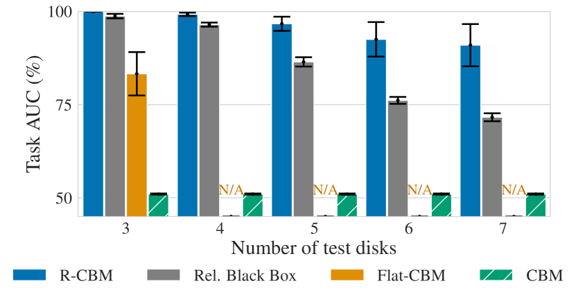
Figure 3: Model generalization on Hanoi OOD on the number of disks. Only R-CBMs are able to generalize effectively to settings larger than the ones they are trained on.

Relational CBMs generalize in relational tasks (Tab. 1)

Relational concept-based models (R-CBMs) match the generalization performance of relational black-box models (e.g., GNNs and KGEs) in relational tasks. In direct comparison, relational CBMs exhibit gains of up to $7\%$ MRR (Countries S1), and at most a $1\%$ loss in accuracy (Citeseer) w.r.t. relational black-boxes. This result directly emerges from R-CBMs’ dynamic architecture allowing them to effectively model concepts and tasks relying on multiple entities. However, simple relational CBMs employing a simple linear layer as task predictor (R-CBM Linear) may still underfit tasks depending on non-linear combinations of concepts (e.g., RPS). In such scenarios, using a deeper task predictor (e.g., R-CBMs Deep) trivially solves the issue, but it also hampers interpretability. Relational DCRs address this limit providing accurate predictions while generating high-quality rule-based explanations (Tab. 3). It also matches generalization performance of the state-of-the-art neural symbolic system DeepStochLog (Winters et al. 2022)), which is provided with ground truth rules.

Table 2: CBMs response to interventions. Relational CBMs effectively respond to human interventions.

	RPS		Hanoi
	Before Interv.	After Interv.	Before Interv.	After Interv.
R-CBM Linear	$49.46\pm 1.11$	$47.83\pm 2.19$	$49.26\pm 1.01$	$\mathbf{100.00\pm 0.00}$
R-CBM Deep	$51.35\pm 2.00$	$82.02\pm 6.34$	$50.07\pm 0.74$	$\mathbf{100.00\pm 0.00}$
R-DCR	$\mathbf{54.47\pm 1.64}$	$\mathbf{100.00\pm 0.00}$	$49.48\pm 0.35$	$\mathbf{100.00\pm 0.00}$
CBM Linear	$49.41\pm 0.89$	$47.75\pm 1.81$	$50.01\pm 0.16$	$55.03\pm 0.53$
CBM Deep	$50.83\pm 0.93$	$47.78\pm 1.94$	$\mathbf{50.44\pm 0.46}$	$60.14\pm 0.46$
DCR	$51.22\pm 1.26$	$49.07\pm 1.60$	$50.00\pm 0.00$	$50.00\pm 0.00$

Relational CBMs generalize in out-of-distribution settings where the number of entities changes at test time (Fig. 3)

Relational CBMs show robust generalization performances even in out-of-distribution conditions where the number of entities varies between training and testing. To assess generalization in these extreme conditions, we use the Tower of Hanoi dataset, where test sets of increasing complexity are generated by augmenting the number of disks in a tower. We observe that a naive approach, such as Flat-CBMs, immediately breaks as soon as we introduce a new disk in a tower, as its architecture is designed for a fixed number of input entities. In contrast, relational CBMs are far more resilient, as we observe a smooth performance decline from $\sim 100\%$ ROC-AUC (with 3 disks in both training and test sets) to around $\sim 85\%$ in the most challenging conditions (with 3 disks in the training set and 7 in the test set).

6.2 Interpretability

Table 3: Rules extracted by relational DCRs. In Hanoi, we remove negative atoms for brevity.

Dataset	Examples of learnt rules
RPS	$\forall v,\exists u.\ wins(v)\leftarrow\neg rock(v)\land paper(v)\land\neg scissors(v)\land rock(u)\land\neg paper(u)\land\neg scissors(u)$
	$\forall v,\exists u.\ loses(v)\leftarrow\neg rock(v)\land\neg paper(v)\land scissors(v)\land rock(u)\land\neg paper(u)\land\neg scissors(u)$
	$\forall v,\exists u.\ ties(v)\leftarrow rock(v)\land\neg paper(v)\land\neg scissors(v)\land rock(u)\land\neg paper(u)\land\neg scissors(u)$
Hanoi	$\forall v,\exists u_{1},u_{2}.\ correct(v)\leftarrow top(u_{1},v)\land top(v,u_{2})\land larger(v,u_{1})\land larger(u_{2},v)\land larger(u_{2},u_{1})$
	$\forall v,\exists u_{1},u_{2}.\ correct(v)\leftarrow top(v,u_{2})\land top(u_{1},u_{2})\land top(u_{2},u_{1})\land larger(v,u_{2})\land larger(u_{2},v)$
Cora	$\forall v,\exists u.\ nn(v)\leftarrow nn(u)\land\neg rl(u)\land\neg rule(u)\land\neg probModels(u)\land\neg theoru(u)\land\neg gene(u)\quad[cite(v,u)]$
PubMed	$\forall v,\exists u.\ type1(v)\leftarrow type1(u)\land\neg type2(u)\land\neg experimental(u)\quad[cite(v,u)]$
Countries	$\forall v_{1},v_{2},\exists u.\ locatedIn(v_{1},v_{2})\leftarrow locatedIn(v_{1},u)\land locatedIn(u,v_{2})$

Table 4: Data efficiency (Citeseer dataset). Relational CBMs are more robust than an equivalent relational black-box when reducing the amount of supervised training nodes.

% Supervision	100%	75%	50%	25%
Rel. Black-Box	$\mathbf{68.32\pm 0.71}$	$66.02\pm 0.67$	$46.46\pm 2.01$	$7.70\pm 0.0$
R-CBM Linear	$67.16\pm 2.05$	$65.96\pm 0.87$	$\mathbf{57.07\pm 3.74}$	$\mathbf{16.92\pm 4.83}$
R-CBM Deep	$66.92\pm 0.75$	$64.08\pm 1.99$	$56.59\pm 1.05$	$12.25\pm 3.53$
R-DCR	$66.89\pm 1.52$	$\mathbf{66.42\pm 1.66}$	$52.30\pm 3.15$	$16.52\pm 1.29$

Relational CBMs support effective interventions (Tab. 2)

A key property of CBM architectures is that allows human interaction with the learnt concepts. This interaction typically involves human experts intervening on mispredicted concepts during testing to improve the final predictions. In our experiments we assess CBMs’ response to interventions on RPS and Hanoi datasets. We set up the evaluation by generating a batch of adversarial test samples that prompt concept encoders to mispredict $\sim 50\%$ of concept labels by introducing a strong random noise in the input features drawn from the uniform distribution $\mathcal{U}(0,20)$. This sets the stage for a comparison between task performances before and after applying interventions. In our findings, we note that relational CBMs positively respond to test-time concept interventions by increasing their task performance. This contrasts with standard CBMs, where even perfect concept predictions are not enough to solve the relational task. Notably, the RPS dataset poses a significant challenge for relational CBMs equipped with linear task predictors, as the task depends on a non-linear combination of concepts. Expanding our investigation to DCRs, we expose another dimension of human-model interaction: rule interventions. Applying both concept and rule interventions, we observe that relational DCRs perfectly predict all adversarial test samples.

Relational Concept Reasoners discover semantically meaningful logic rules (Tab. 3)

Among CBMs, the key advantage of DCRs lies in the dual role of generating rules which serve for both generating and explaining task predictions. We present instances of relational DCR explanations in Tab. 3. Our results demonstrate that relational DCRs discover rules aligned with known ground truths across diverse datasets (e.g., $wins(X)\leftarrow\neg rock(X)\land paper(X)\land\neg scissors(X)\land rock(Y)\land\neg paper(Y)\land\neg scissors(Y)$ in RPS). Notably, relational DCRs discover meaningful rules even when exact ground truth rules are unknown, such as in Cora, Citeseer and PubMed. Finally, relational DCRs are capable to unveil meaningful rules even under minimal concept supervisions (R-DCR Low).

6.3 Low data regimes

Relational CBMs generalize better than relational black-boxes in low-data regimes (Tab. 4)

Relational CBMs surpass relational black box models when dealing with limited data. Specifically, we evaluated the ability of relational CBMs and relational black box models to generalize on the Citeseer dataset as the number of labeled nodes decreased to 75%, 50%, and 25%. While no significant difference was observed with ample training data, a growing disparity emerged between relational CBMs and relational black box models in scenarios of scarce data. The intermediate predictions related to concepts likely have a crucial regularization effect, particularly in scenarios with limited data.

Relational DCRs accurately make interpretable task predictions with very few concept supervisions (Tab. 1)

When forced to make very crisp decisions on concepts, i.e. $g_{i}(\bar{x})$ (see Appendix B), R-DCR Low is able to learn an interpretable relational task predictor by accessing only to 5 labelled examples at the concept level. While these labeled examples are not essential for achieving strong generalization, supervision becomes crucial to establish an alignment between human and model on the semantics of the concepts and of the associated logical explanations. The alignment can be perfectly achieved in RPS, where concepts possess a mutually exclusive structure. On the Hanoi dataset, learning the relational binary concepts $larger$ and $top$ from 5 examples only proves more challenging, leading to slightly decreased overall performance.

7 Discussion

Relations with CBMs.

Concept-based models (Koh et al. 2020) quickly inspired several works aimed at improving their generalization (Mahinpei et al. 2021; Espinosa Zarlenga et al. 2022; Vielhaben, Bluecher, and Strodthoff 2023), explanations (Ciravegna et al. 2023; Barbiero et al. 2023), and robustness (Marconato, Passerini, and Teso 2022; Havasi, Parbhoo, and Doshi-Velez 2022; Zarlenga et al. 2023; Kim et al. 2023). Despite these efforts, the application of CBMs to relational domains currently remained unexplored. Filling this gap, our framework allows relational CBMs to (i) effectively solve relational tasks, and (ii) elevate the explanatory expressiveness of these models from propositional to relational explanations.

Relations with GNNs.

Relational CBMs and relational black-boxes (such as GNNs) share similarities in considering the relationships between multiple entities when solving a given task. More specifically, in relational CBMs the task aggregation resembles existing relational paradigms such as message-passing in graph neural networks (Gilmer et al. 2017), which is used to aggregate messages from entities’ neighborhoods. However, the key difference is that relational CBMs apply this aggregation on a semantically meaningful set of concepts (instead of embeddings), allowing the extraction of concept-based explanations (as opposed to graph neural networks).

Limitations

The main limitation of relational CBMs consists in their limited scalability to very large domains, akin to all existing relational systems (even outside deep learning and AI). Extensions of relational CBMs may include automating the generation of relational templates $b$, the calibration of template widths $w$, and the construction of reduced set of variables’ substitutions $\Theta$.

Conclusions

This work presents relational CBMs, a family of concept-based models specifically designed for relational tasks while providing simple explanations for task predictions. The results of our experiments show that relational CBMs: (i) match the generalization performance of existing relational black-boxes (as opposed to non-relational CBMs), (ii) support the generation of quantified concept-based explanations, (iii) effectively respond to test-time interventions, and (iv) withstand demanding settings including out-of-distribution scenarios, limited training data regimes, and scarce concept supervisions. While relational CBMs already represent a significant extension of standard CBMs, they also pave the way to further investigate the extension of CBMs as a way to improve interpretability in GNNs and to explain KGE predictions.

Appendix A Datasets

A.1 Rock-Paper-Scissors

We build the Rock-Paper-Scissors (RPS) dataset by downloading images from Kaggle: https://www.kaggle.com/datasets/drgfreeman/rockpaperscissors?resource=download. The dataset contains images representing the characteristic hand-signs annotated with the usual labels ”rock”, ”paper”, and ”scissors”. To build a relational dataset we randomly select $200$ pairs of images and defined the labels wins/ties/loses according to the standard game-play. To train the models we select an embedding size of $10$.

A.2 Tower of Hanoi

We build the Tower of Hanoi (Hanoi) dataset by generating disk images with matplotlib. We randomly generate $1000$ images representing disks of different sizes in $[1,10]$ and at different heights of the tower in $[1,10]$. We annotate the concepts $top(u,v),larger(u,v)$ using pairs of disks according to the usual definitions. We define the task label of each disk according to whether the disk is well positioned following the usual definition that a disk is well positioned if the disk below (if any) is larger, and the disk above (if any) is smaller. To train the models we select an embedding size of $50$.

A.3 Cora, Citeseer, PubMed, Countries

For the experiments in Tab 1, we exploit the standard splits of the Planetoid Cora, Citeseer and PubMed citation networks, as defined in Pytorch Geometric https://pytorch-geometric.readthedocs.io/en/latest/modules/datasets.html. The classes of documents are used both for tasks and concepts

The Countries dataset (ODbL licence) defines a set of countries, regions and sub-regions as basic entities. We used splits and setup from Rocktaschel et al. (Rocktäschel and Riedel 2017), which reports the basic statistics of the dataset and also defines the tasks S1, S2 used in this paper.

Appendix B Baselines

B.1 Exploiting prior knowledge

Additionally, we can use prior knowledge to optimize the template and the aggregation by excluding concept atoms in $b(\bar{v},\bar{u})$ and groundings in $\Theta$ that are not relevant to predict the task. This last simplification is crucial anytime we want to impose a locality bias, and it is also at the base of the heuristics that are commonly used in extension of knoweldge graph embeddings with additional knowledge (Qu et al. 2020; Zhang et al. 2020; Diligenti et al. 2023).

B.2 Cora, Citeseer, PubMed

Slash notation $a/b/c$ indicates parameters for $cora/citeseer/pubmed$ when different.

R-CBMs exploit the same concept encoder $g_{i}$, which corresponds to an MLP with 2 hidden layers of size $32/16/16$ followed by an output layer of size $6/7/3$ classes. Activation functions are LeakyReLu. The blackbox feedforward network is equivalent to the one of the CBM models. The blackbox relational model is a GCN with 2 layers of size 16. Node features for R-CBM models are initialized with the last embeddings of the GCN. R-CMB Deep task predictor exploits a 2 layer MLP with 1 hidden layers of size $32/16/16$ followed by an output layer of size $1$. Activation functions are LeakyReLu. R-DCR exploits, as $filter$ and $sign$ functions a linear layer of size $32/16/16$. DeepStochLog exploits the same concept encoder as neural predicate. It exploits also the pretraining using a GCN. As task predictor, it exploits a SDCG grammar implementing the rule $cite(v_{1},v_{2})\rightarrow class_{i}(v_{1})\iff class_{i}(v_{2})$.

B.3 Countries

The DistMult Knowledge Graph Embeddings (KGE) (Yang et al. 2014) was used as BlackBox relational baseline for the Countries S1 and S2 datasets. We varied the embedding sizes in the set $\{10,20,50,100,200,300\}$ and selected the best results on the validation set. The DistMult KGE was used as a basic concept encoder for CMBs. The R-CBM linear computes the concepts via linear layer followed by the KGE output layer. The R-CBM Deep computes the concepts via an MLP with 2 hidden layers followed by a KGE output layer. Activation functions are ReLu.

Appendix C Experimental Details and Additional experiments

C.1 Training Hyperparameters

In all synthetic tasks, we generate datasets with 3,000 samples and use a traditional 70%-10%-20% random split for training, validation, and testing datasets, respectively. During training, we then set the weight of the concept loss to $\lambda=0.1$ across all models. We then train all models for $3000$ epochs using full batching and a default Adam (Kingma and Ba 2014) optimizer with learning rate $10^{-4}$.

C.2 Data Efficiency

As explained in Section B.2, the relational CBMs exploits the features obtained by pretraining on a GNN on the same data split. Such pretraining is beneficial only in high-data settings (i.e. 100%, 75% and 50%). On low data regime (i.e. 25%), pretrained features are worse than original features. In these cases, we train the different baselines from scratch by using directly the low level features of the documents.

C.3 Countries

The task consists of predicting the unknown locations of a country, given the evidence in form of country neighbourhoods and some known country/region locations. The entities are divided into the $C,R,W$ domains referring to the countries, regions and continents, respectively. The predicate $locIn(v_{1},v_{2})$ determines the location of a country in a region or continent, with the variables $(v_{1},v_{2})\in C\times R\cup W$ or $(v_{1},v_{2})\in R\times W$. The country neighbourhoods are determined by the predicate $neighOf(v_{1},v_{3})$ with the variables $v_{1},v_{3}\in C$.

The entities in the dataset are a set of countries, regions and continents represented by their corresponding feature vectors as computed by a DistMult KGE (see baselines). The concept datasets are respectively the set $D_{c_{locIn}}=(C\times R)\cup(R\times W)$ and $D_{c_{neighOf}}=C\times C$. The task dataset $D_{y_{locIn}}=C\times W$ is formed by queries about the location of some countries within a continent. The task template is defined as:

$$\begin{array}[]{l}locIn(v_{1},v_{2})\mathop{:\!\!-}locIn(v_{1},u_{1}),locIn(u_{1},v_{2}),\\ neighOf(v_{1},u_{2}),locIn(u_{2},v_{2}),\ \forall u_{1}\in R,u_{2}\in C\ .\end{array}$$

Finally, the cross entropy loss was used both for functions for concepts.

Appendix D Relational Task Predictors

In standard CBMs, a wide variety of task predictors $f$ have been proposed on top of the concept encoder $g$, defining different trade-offs between model accuracy and interpretability. In the following, we resume how we adapted a selection of representative models for $f$ to be applicable in a relational setting (fixing for simplicity $o=0$). These are the models that we will compare in the experiments (Sections 5 and 6).

Relational Concept-based Model Linear (R-CBM Linear)

The most basic task predictor employed in standard CBMs is represented by a single linear layer (Koh et al. 2020). This choice guarantees a high-degree of interpretability, but may lack expressive power and may significantly underperform whenever the task depends on a non-linear combination of concepts. In the relational context, we define it as following:

$$f(\theta_{\bar{u}}b(\bar{x},\bar{u}))=W\theta_{\bar{u}}b(\bar{x},\bar{u})+w_{0}$$ (7)

Deep Relational Concept-based Model (Deep R-CBM)

To solve the linearity issue of R-CBM, one can increase the number of layers employed by the task predictor (as also proposed in Koh et al. (2020)). In the relational context we can define a Deep R-CBM as following:

$$\text{Deep R-CBM:}\quad f(\theta_{\bar{u}}b(\bar{x},\bar{u}))=\varphi(\theta_{\bar{u}}b(\bar{x},\bar{u})),$$ (8)

where we indicate with $MLP$ a multi-layer perceptron. However, the interpretability between concept and task predictions is lost, since MLPs are not transparent. Further, the ability of a Deep R-CBM to make accurate predictions is totally depending on the existence of concepts that univocally represent the tasks, hence being possibly very inefficacy.

Relational Deep Concept Reasoning (R-DCR)

Espinosa Zarlenga et al. (2022) proposed to encode concepts by employing concept embeddings (instead of just concept scores), improving CBMs generalization capabilities, but affecting their interpretability. Then Barbiero et al. (2023) proposed to use these concept embeddings to generate a symbolic rule which is then executed on the concept scores, providing a completely interpretable prediction. We adapt this model in the relational setting:

$$\text{R-DCR:}\quad f(\theta_{\bar{u}}b(\bar{x},\bar{u}))=\varphi(\theta_{\bar{u}}b(\bar{x},\bar{u})),$$ (9)

where $\varphi$ indicates the rule generated by a neural module working on the concept embeddings. For further details on how $\varphi$ is learned, please refer to (Barbiero et al. 2023). Since the logical operations in R-DCR are governed by a semantics specified by a t-norm fuzzy logic (Hájek 2013), whenever we use this model we require the aggregation operation $\oplus$ used in /Eq. 5 to correspond to a fuzzy OR. The $\max$ operator corresponds to the OR within the Gödel fuzzy logic.

R-DCR Low

R-DCR Low is a version of R-DCR that is trained by providing the concept supervision of only 5 supervised examples. Its architecture and learning is entirely identical to DCR except for two variants:

• Since DCR strongly depends on crisp concepts prediction for learning good and interpretable rule, in absence of sufficient supervision, we need a different way to obtain crisp predictions. To this end we substitute the standard sigmoid and softmax activation functions for concept predictors $g_{i}$ with discrete differentiable sample from a bernoulli or categorial distributions. The differentiability is obtained by using the Straight Through estimators provided by PyTorch.

• Since the backward signal from DCR can be very noisy at the beginning of the learning, we add a parallel task predictor (and a corresponding loss term), completely identical to the one of a R-CBM Deep model. Such predictor only guides the learning of the concepts during training by a cleaner backward signal but is discarded during test, leaving a standard DCR architecture.

Flat Concept-based Model (Flat CBM) assumes each task to be computed as a function of the full set of ground concept atoms, as described in the template in Eq. 3. We only introduce this model for comparison reasons in the experimental section.

Appendix E Code, Licences, Resources

Libraries

For our experiments, we implemented all baselines and methods in Python 3.7 and relied upon open-source libraries such as PyTorch 1.11 (Paszke et al. 2019) (BSD license) and Scikit-learn (Pedregosa et al. 2011) (BSD license). To produce the plots seen in this paper, we made use of Matplotlib 3.5 (BSD license). We will release all of the code required to recreate our experiments in an MIT-licensed public repository.

Resources

All of our experiments were run on a private machine with 8 Intel(R) Xeon(R) Gold 5218 CPUs (2.30GHz), 64GB of RAM, and 2 Quadro RTX 8000 Nvidia GPUs. We estimate that approximately 50-GPU hours were required to complete all of our experiments.

References

- Barbiero et al. (2023) Barbiero, P.; Ciravegna, G.; Giannini, F.; Zarlenga, M. E.; Magister, L. C.; Tonda, A.; Lio, P.; Precioso, F.; Jamnik, M.; and Marra, G. 2023. Interpretable Neural-Symbolic Concept Reasoning. arXiv preprint arXiv:2304.14068.
- Ciravegna et al. (2023) Ciravegna, G.; Barbiero, P.; Giannini, F.; Gori, M.; Lió, P.; Maggini, M.; and Melacci, S. 2023. Logic explained networks. Artificial Intelligence, 314: 103822.
- Diligenti et al. (2023) Diligenti, M.; Giannini, F.; Fioravanti, S.; Graziani, C.; Falaschi, M.; and Marra, G. 2023. Enhancing Embedding Representations of Biomedical Data using Logic Knowledge. arXiv preprint arXiv:2303.13566.