Non-ergodic linear convergence property of the delayed gradient descent under the strongly convexity and the Polyak-Łojasiewicz condition

Abstract.

In this work, we establish the linear convergence estimate for the gradient descent involving the delay $\tau\in\mathbb{N}$ when the cost function is $\mu$-strongly convex and $L$-smooth. This result improves upon the well-known estimates in Arjevani et al. [2] and Stich-Karmireddy [11] in the sense that it is non-ergodic and is still established in spite of weaker constraint of cost function. Also, the range of learning rate $\eta$ can be extended from $\eta\leq 1/(10L\tau)$ to $\eta\leq 1/(4L\tau)$ for $\tau=1$ and $\eta\leq 3/(10L\tau)$ for $\tau\geq 2$, where $L>0$ is the Lipschitz continuity constant of the gradient of cost function. In a further research, we show the linear convergence of cost function under the Polyak-Łojasiewicz (PL) condition, for which the available choice of learning rate is further improved as $\eta\leq 9/(10L\tau)$ for the large delay $\tau$. Finally, some numerical experiments are provided in order to confirm the reliability of the analyzed results.

1. Introduction

In this paper, we consider the gradient descent with a fixed delay $\tau\in\mathbb{N}$ in the optimization problem:

$$x_{t+1}=\left\{\begin{aligned} &x_{t}-\eta\nabla f(x_{t-\tau})&&\textrm{~{}for~{}}~{}t\geq\tau,\\ &x_{0}&&\textrm{~{}for~{}}~{}0\leq t<\tau,\end{aligned}\right.$$ (1.1)

where the given cost $f:\mathbb{R}^{d}\rightarrow\mathbb{R}$ is a differentiable convex function and the initial point $x_{0}\in\mathbb{R}^{d}$ is given. Throughout this paper, denote by $x_{*}\in\mathbb{R}^{d}$ a unique minimizer of the cost function $f$.

The gradient descent scheme (1.1) has gained a lot of interest from many researchers since it has a simple form among the gradient descent algorithms involving the delay which naturally appear in various learning problems such as the asynchronous gradient descent and the multi-agent optimization. So far, numerous related studies have been investigated. The delay effect in the stochastic gradient descent was studied in several literatures [2, 6, 8, 11, 12, 17], and moreover, some studies of the delay effect of communication in the decentralized optimization could be found in the references [1, 14, 15]. Also, the online problem involving the feedback delay was studied in [4, 5, 7, 9, 13, 15, 16]. Understanding the convergence analysis of (1.1) will be fundamentally important, as it serves as the foundation for numerous other related algorithms employed in the aforementioned applications.

This paper concerns the linear convergence property of (1.1). We first recall two previous basic results of [2] and [11] in this line of research. Arjevani et al. [2] provided the following linear convergence result when the cost is given by a strongly convex quadratic function.

Theorem 1.1 ([2]).

Assume that $f:\mathbb{R}^{d}\rightarrow\mathbb{R}$ is $\mu$-strongly convex and $L$-smooth, and suppose that $f$ is given as $f(x)=2^{-1}\,x^{T}Ax+b^{T}x+c$ for some $A\in\mathbb{R}^{d\times d}$, $b\in\mathbb{R}^{d}$ and $c\in\mathbb{R}$. Then, for a positive stepsize $\eta\leq\frac{1}{20L(\tau+1)}$ it holds that

$$f(x_{t})-f(x_{*})\leq 5L(1-\mu\eta)^{2t}\|x_{0}-x_{*}\|^{2}\qquad\forall\,t\geq 0.$$

As for the general strongly convex and smooth cost functions, Stich and Karimireddy [11] showed the following ergodic type result:

Theorem 1.2 ([11]).

Assume that $f:\mathbb{R}^{d}\rightarrow\mathbb{R}$ is $\mu$-strongly convex and $L$-smooth. There exists a positive stepsize $\eta\leq\frac{1}{10L\tau}$ such that

$${\mathbb{E}\Big{(}f(x^{out})-f(x_{*})\Big{)}}=O\Big{(}L\tau\|x_{0}-x_{*}\|^{2}\exp\Big{[}-\frac{\mu T}{10L\tau}\Big{]}\Big{)}\qquad\forall\,T\geq 1,$$

where the expectation is given for the variable $x^{out}\in\{x_{t}\}_{t=0}^{T-1}$ which is chosen to be $x_{t}$ with probability proportional to $(1-\mu\eta/2)^{-t}$.

The aim of this paper is to improve the aforementioned results in following senses: First, we obtain a non-ergodic linear convergence property of (1.1) when $f$ is $\mu$-strongly convex and $L$-smooth. Second, our linear convergence result permits a larger range of the stepsize $\eta>0$ than the results of [2, 11].

We first state the brief version of our main result with the linear convergence.

Theorem 1.3.

Assume that $f:\mathbb{R}^{d}\rightarrow\mathbb{R}$ is $\mu$-strongly convex and $L$-smooth. Then, for any choice of stepsize $\eta$ satisfying

$$0<\eta\leq\frac{C_{\tau}}{L\tau},$$ (1.2)

the sequence $\{x_{t}\}_{t\geq 0}$ of (1.1) satisfies the following estimate:

$$\|x_{t}-x_{*}\|\leq\frac{1}{1-J_{\tau/2}L\tau\eta}\Big{(}1-\frac{\eta\alpha}{2}\Big{)}^{t/2}\|x_{0}-x_{*}\|\qquad\forall\,t\geq 0,$$ (1.3)

where $C_{\tau}:=\frac{\tau}{\sqrt{6J_{\tau}\tau^{2}+1}+1}$ and $\alpha:=\frac{2\mu L}{\mu+L}$ with a constant $J_{n}$ for $n\in\{k/2\mid k\in\mathbb{N}\}$ given by

$$J_{n}=\left\{\begin{array}[]{ll}1.455&\quad\textrm{for }~{}n=1/2,\\ 1.25&\quad\textrm{for }~{}n=1,\\ 1.2&\quad\textrm{for }~{}n\geq 3/2.\end{array}\right.$$ (1.4)

Remark 1.4.

We briefly describe their numeric values and boundness of some constants used in Theorem 1.3.

1. The value of $C_{\tau}$ increases in $\tau$ and $\lim_{\tau\rightarrow\infty}C_{\tau}=1/\sqrt{7.2}\simeq 0.3727$. In Table 1, we provide more numeric values of $C_{\tau}$ up to $\tau=8$ for the sake of convenience.

   $\tau$	1	2	3	4	5	6	7	8
   $C_{\tau}$	0.2553	0.3096	0.3292	0.3396	0.3459	0.3502	0.3534	0.3557

   Table 1. Numeric values of $C_{\tau}$ up to $\tau=8$

2. We note that the coefficient $\frac{1}{1-J_{\tau/2}L\tau\eta}$ in (1.3) approaches to $1$ as $\tau\rightarrow 0$. Furthermore, since $J_{\tau/2}L\tau\eta\leq J_{\tau/2}C_{\tau}<1/2$ for all $\tau\geq 1$, one sees that

   $$0<\frac{1}{1-J_{\tau/2}L\tau\eta}<2\qquad\mbox{ for }~{}\eta\leq\frac{C_{\tau}}{L\tau}.$$

Next, we give the generalized result of Theorem 1.3.

Theorem 1.5.

Assume that $f:\mathbb{R}^{d}\rightarrow\mathbb{R}$ is $\mu$-strongly convex and $L$-smooth. If we choose the stepsize $\eta>0$ satisfying

$$\eta\leq\min\Bigg{\{}\frac{L(1+q)}{5\alpha},~{}\frac{\tau}{\sqrt{2J_{\tau}\tau^{2}(2+1/q)+1}+1}\Bigg{\}}\frac{1}{\tau L},$$ (1.5)

then the sequence $\{x_{t}\}_{t\geq 0}$ of (1.1) satisfies

$$\|x_{t}-x_{*}\|\leq\frac{1}{1-J_{\tau/2}L\tau\eta}\left(1-\frac{\eta\alpha}{1+q}\right)^{t/2}\|x_{0}-x_{*}\|\qquad\forall\,t\geq 0,$$ (1.6)

where $q>0$ is a chosen constant and $\alpha:=\frac{2\mu L}{\mu+L}$. In particular, since $\frac{L}{\alpha}\geq 1$ due to $L\geq\mu$, Theorem 1.3 is also satisfied with $q=1$.

In fact, the number $q>0$ in Theorem 1.5 appears in the progress of applying Young’s inequality in the proof of Proposition 2.1. Actually, we observe that if one choose a large $q>0$, then the range of $\eta$ in (1.5) becomes larger with an upper bound while the diminishing factor in the decay estimate (1.6) becomes close to one. Contrary, if we choose a small $q>0$, then the diminishing factor in (1.6) becomes small but the range of $\eta$ in (1.5) is more restricted.

For the proof of Theorem 1.5, we will consider an auxiliary sequence $\{\tilde{x}_{t}\}$, which was also utilized in the previous work [11]. Using the smoothness and the strongly convexity of the function $f$, we will obtain a sequential inequality of the error $\|\tilde{x}_{t}-x_{*}\|$. We will then analyze the sequential inequality carefully to obtain a linear convergence estimate of the error $\|\tilde{x}_{t}-x_{*}\|$. So, it will be done by using Lemma 2.2 which is one of the main technical contributions of this paper. Afterwards, using the derived estimate of $\|\tilde{x}_{t}-x_{*}\|$ and measuring the difference between $x_{t}$ and $\tilde{x}_{t}$, we will finally show a linear convergence result of the error $\|x_{t}-x_{*}\|$.

On the other hand, we next derive a linear convergence result when the cost function satisfies the following Polyak-Łojasiewicz (PL) condition: There exists a number $\zeta>0$ such that

$$\frac{1}{2}\|\nabla f(x)\|^{2}\geq\zeta\Big{(}f(x)-f_{*}\Big{)},$$ (1.7)

where $f_{*}$ is the minimal value of $f$, i.e., $f_{*}=f(x_{*})$.

Theorem 1.6.

Suppose that $f:\mathbb{R}^{d}\rightarrow\mathbb{R}$ is $L$-smooth and it satisfies the PL condition (1.7). If we assume that the stepsize $\eta>0$ and the delay $\tau>0$ satisfy the following inequality:

$$\eta\leq\min\Big{\{}\frac{L}{5\zeta},~{}\frac{2\tau}{\sqrt{1+4J_{\tau}\tau^{2}}+1}\Big{\}}\frac{1}{L\tau},$$ (1.8)

then for any $t\geq\tau$ we have

$$f(x_{t})-f_{*}\leq\left(1-{\eta\zeta}\right)^{t-\tau}\Big{(}f(x_{\tau})-f_{*}\Big{)}.$$ (1.9)

In order to prove Theorem 1.6, we will meet a sequence inequality in terms of the sequence $\{f(x_{t})-f_{*}\}_{t\geq\tau}$ similar to the one appeared in the proof of Theorem 1.5. We will then use the result of Lemma 2.3 to analyze the concerned sequence. Interestingly, its proof does not use the auxiliary sequence $\{\tilde{x}_{t}\}$ anymore, and so it is simpler than the proof of Theorem 1.5.

The rest of this paper is organized as follows. In Section 2, we define an auxiliary sequence and show the linear convergence property of its error. With the help of this result, we derive the linearly convergent error estimate of the sequence $\{x_{t}\}_{t\geq 0}$ in Section 3. Also, the linear convergence result under the PL condition is proved in Section 4. Finally, we provide some numerical examples in Section 5 for supporting our analyzed results.

2. Preliminary convergence result

In this section, we discuss a convergence result of an auxiliary sequence $\{\tilde{x}_{t}\}$ satisfying

$$\tilde{x}_{0}=x_{0},\qquad\tilde{x}_{t+1}=\tilde{x}_{t}-\eta\nabla f(x_{t})\qquad\forall\,t\geq 0,$$ (2.1)

where $\{x_{t}\}$ is defined by (1.1). It will play an essential role to obtain the linear convergence estimate (1.6) (cf. [11]). Throughout Section 2-3, it is assumed that the cost function $f$ satisfies the following two assumptions:

Assumption 1.

The function $f$ is $L$-smooth, defined as follows: There is a number $L>0$ such that

$$\|\nabla f(y)-\nabla f(x)\|\leq L\|y-x\|\qquad\forall\,x,\,y\in\mathbb{R}^{d}.$$ (2.2)

Assumption 2.

The function $f$ is $\mu$-strongly convex, defined as follows: There is a number $\mu>0$ such that

$$f(y)\geq f(x)+(y-x)^{T}\cdot\nabla f(x)+\frac{\mu}{2}\|y-x\|^{2}\qquad\forall\,x,\,y\in\mathbb{R}^{d}.$$ (2.3)

We state an intermediate inequality regarding the quantity $\|\tilde{x}_{t}-x_{*}\|$.

Proposition 2.1.

Let $\tilde{x}_{t}$ be an auxiliary sequence defined by (2.1). For the minimizer $x_{*}\in\mathbb{R}$ of the given cost function $f$, we obtain

$$\begin{split}&\|\tilde{x}_{t+1}-x_{*}\|^{2}\\ &\leq\Big{(}1-\frac{\alpha\eta}{1+q}\Big{)}\|\tilde{x}_{t}-x_{*}\|^{2}-\Big{(}\frac{\eta}{2L}-\eta^{2}\Big{)}\|\nabla f(x_{t})\|^{2}+\eta^{2}\tau\Big{(}\frac{\alpha\eta}{q}+2L\eta\Big{)}\mathcal{R}(t),\end{split}$$ (2.4)

where $\alpha:=\frac{2\mu L}{\mu+L}$, $q>0$ is a constant and

$$\mathcal{R}(t):=\left\{\begin{array}[]{ll}0&\textrm{ if }~{}t=0,\\ \sum_{j=0}^{t-1}\|\nabla f(x_{j})\|^{2}&\textrm{ if }~{}1\leq t\leq\tau,\\ \sum_{j=t-\tau}^{t-1}\|\nabla f(x_{j})\|^{2}&\textrm{ if }~{}t\geq\tau+1.\end{array}\right.$$ (2.5)

Proof.

The definition of $\tilde{x}_{t}$ in (2.1) implies

$$\begin{split}&\|\tilde{x}_{t+1}-x_{*}\|^{2}\\ &=\|\tilde{x}_{t}-x_{*}-\eta\nabla f(x_{t})\|^{2}\\ &=\|\tilde{x}_{t}-x_{*}\|^{2}-2\eta\langle\tilde{x}_{t}-x_{*},\nabla f(x_{t})\rangle+\eta^{2}\|\nabla f(x_{t})\|^{2}\\ &=\|\tilde{x}_{t}-x_{*}\|^{2}-2\eta\langle{x}_{t}-x_{*},\nabla f(x_{t})\rangle+\eta^{2}\|\nabla f(x_{t})\|^{2}+2\eta\langle x_{t}-\tilde{x}_{t},~{}\nabla f(x_{t})\rangle.\end{split}$$ (2.6)

By the strongly convexity and the $L$-smoothness property, we have

$$\langle x_{t}-x_{*},\nabla f(x_{t})\rangle\geq\frac{\mu L}{\mu+L}\|x_{t}-x_{*}\|^{2}+\frac{1}{\mu+L}\|\nabla f(x_{t})\|^{2}.$$ (2.7)

Applying (2.7) to (2.6), one yields

$$\begin{split}&\|\tilde{x}_{t+1}-x_{*}\|^{2}\\ &\leq\|\tilde{x}_{t}-x_{*}\|^{2}-{\alpha\eta}\|x_{t}-x_{*}\|^{2}-\Big{(}\frac{2\eta}{\mu+L}-\eta^{2}\Big{)}\|\nabla f(x_{t})\|^{2}+2\eta\langle x_{t}-\tilde{x}_{t},~{}\nabla f(x_{t})\rangle.\end{split}$$ (2.8)

By Young’s inequality, we easily note that

$$2\eta\langle x_{t}-\tilde{x}_{t},~{}\nabla f(x_{t})\rangle\leq\frac{\eta}{2L}\|\nabla f(x_{t})\|^{2}+2L\eta\|x_{t}-\tilde{x}_{t}\|^{2},$$

and again, applying this result to (2.8), we have

$$\begin{split}&\|\tilde{x}_{t+1}-x_{*}\|^{2}\\ &\leq\|\tilde{x}_{t}-x_{*}\|^{2}-{\alpha\eta}\|x_{t}-x_{*}\|^{2}-\Big{(}\frac{2\eta}{\mu+L}-\eta^{2}-\frac{\eta}{2L}\Big{)}\|\nabla f(x_{t})\|^{2}+2L\eta\|x_{t}-\tilde{x}_{t}\|^{2}\\ &\leq\|\tilde{x}_{t}-x_{*}\|^{2}-{\alpha\eta}\|x_{t}-x_{*}\|^{2}-\Big{(}\frac{\eta}{2L}-\eta^{2}\Big{)}\|\nabla f(x_{t})\|^{2}+2L\eta\|x_{t}-\tilde{x}_{t}\|^{2},\end{split}$$ (2.9)

where the last inequality is obtained by using $\frac{2\eta}{\mu+L}\geq\frac{\eta}{L}$ due to $\mu\leq L$. Since

$$(1+q)\|x_{t}-x_{*}\|^{2}+\Big{(}1+\frac{1}{q}\Big{)}\|\tilde{x}_{t}-x_{t}\|^{2}\geq\|\tilde{x}_{t}-x_{*}\|^{2}\qquad\mbox{ for }~{}q>0,$$

the inequality (2.9) becomes

$$\begin{split}&\|\tilde{x}_{t+1}-x_{*}\|^{2}\\ &\leq\Big{(}1-\frac{\alpha\eta}{1+q}\Big{)}\|\tilde{x}_{t}-x_{*}\|^{2}-\Big{(}\frac{\eta}{2L}-\eta^{2}\Big{)}\|\nabla f(x_{t})\|^{2}+\Big{(}\frac{\alpha\eta}{q}+2L\eta\Big{)}\|x_{t}-\tilde{x}_{t}\|^{2}.\end{split}$$ (2.10)

On the other hand, subtracting (2.1) from (1.1), one gets

$$x_{t+1}-\tilde{x}_{t+1}=x_{t}-\tilde{x}_{t}-\eta\left(\nabla f(x_{t-\tau})-\nabla f(x_{t})\right),$$

and then, this implies

$$x_{t}-\tilde{x}_{t}=\left\{\begin{array}[]{ll}0&\textrm{if }~{}t=0,\\ \eta\sum_{j=0}^{t-1}\nabla f(x_{j})&\textrm{if }~{}0\leq t\leq\tau,\\ \eta\sum_{j=t-\tau}^{t-1}\nabla f(x_{j})&\textrm{if }~{}t\geq\tau+1.\end{array}\right.$$

By Cauchy-Schwartz inequality, we have

$$\|x_{t}-\tilde{x}_{t}\|^{2}\leq\eta^{2}\tau\mathcal{R}(t),$$ (2.11)

where $\mathcal{R}(t)$ is given by (2.5). Applying (2.11) to (2.10), the desired inequality (2.4) is shown. ∎

For simplicity, we let

$$a_{t}=\|\tilde{x}_{t}-x_{*}\|^{2},\qquad b_{t}=\|\nabla f(x_{t})\|^{2}.$$

Then the result (2.4) in Proposition 2.1 is rewritten as

$$a_{t+1}\leq\Big{(}1-\frac{\alpha\eta}{1+q}\Big{)}a_{t}-\Big{(}\frac{\eta}{2L}-\eta^{2}\Big{)}b_{t}+\eta^{2}\tau\Big{(}\frac{\alpha\eta}{q}+2L\eta\Big{)}\mathcal{R}(t).$$ (2.12)

Since $\alpha\leq L$, the inequality (2.12) becomes

$$\begin{split}a_{t+1}\leq&~{}\Big{(}1-\frac{\alpha\eta}{1+q}\Big{)}a_{t}-\Big{(}\frac{\eta}{2L}-\eta^{2}\Big{)}b_{t}\\ &\qquad~{}+\left\{\begin{array}[]{ll}0&\textrm{for }~{}t=0,\\ \delta(b_{t-1}+\cdots+b_{0})&\textrm{for }~{}1\leq t\leq\tau,\\ \delta(b_{t-1}+\cdots+b_{t-\tau})&\textrm{for }~{}t\geq\tau+1,\end{array}\right.\end{split}$$ (2.13)

where $\delta:=\left(2+\frac{1}{q}\right)\eta^{3}\tau L$.

From (2.13), we next establish the estimate of $a_{t}$ in the following lemma.

Lemma 2.2.

Suppose that two positive sequences $\{a_{t}\}_{t\geq 0}$ and $\{b_{t}\}_{t\geq 0}$ satisfy

$$a_{t+1}\leq\left\{\begin{array}[]{ll}ca_{0}-Qb_{0}&\quad\textrm{for }~{}t=0,\\ ca_{t}+\delta(b_{t-1}+\cdots+b_{0})-Qb_{t}&\quad\textrm{for }~{}1\leq t\leq\tau,\\ ca_{t}+\delta(b_{t-1}+\cdots+b_{t-\tau})-Qb_{t},&\quad\textrm{for }~{}t\geq\tau+1,\end{array}\right.$$ (2.14)

where $c$, $\delta$ and $Q$ are some positive constants. If we assume that for any $1\leq j\leq\tau$,

$$\sum_{k=0}^{j-1}c^{k}\delta\leq c^{j}Q,$$ (2.15)

then we have

$$a_{t+1}\leq c^{t+1}a_{0}\qquad\forall\,t\geq 0.$$ (2.16)

Proof.

In this proof, we will show the desired result (2.16) separately considering three cases: $t=0$, $1\leq t\leq\tau$ and $t\geq\tau+1$.

Case 1.  When $t=0$, the inequality (2.14) implies

$$a_{1}\leq ca_{0}-Qb_{0}\leq ca_{0},$$

which directly gives the desired one (2.16) for $t=0$.

Case 2.  We next show (2.16) for $1\leq t\leq\tau$. By (2.14) for $t=0$ and $1$, one has

$$\begin{split}a_{2}&\leq ca_{1}+\delta b_{0}-Qb_{1}\\ &\leq c(ca_{0}-Qb_{0})+\delta b_{0}-Qb_{1}\\ &=c^{2}a_{0}+(\delta-cQ)b_{0}-Qb_{1}.\end{split}$$

Generally, using (2.14) for $0\leq t\leq\tau$ sequentially, we can obtain that for $1\leq t\leq\tau$,

$$a_{t+1} \leq\,c^{t+1}a_{0}+\sum_{j=0}^{t-1}\Big{[}\delta+c\delta+\cdots+c^{t-1-j}\delta-c^{t-j}Q\Big{]}b_{j}-Qb_{t}$$ (2.17)

$$=\,c^{t+1}a_{0}+\sum_{j=0}^{t-1}\left(\sum_{k=0}^{t-1-j}c^{k}\delta-c^{t-j}Q\right)b_{j}-Qb_{t}.$$

This inequality with the condition (2.15) implies that $a_{t+1}\leq c^{t+1}a_{0}$ for $1\leq t\leq\tau$.

Case 3.  For $t\geq\tau+1$, we first claim that

$$\begin{split}a_{t+1}&\leq\,c^{t+1}a_{0}+\sum_{j=t-\tau}^{t-1}\Big{[}\delta+c\delta+\cdots+c^{t-1-j}\delta-c^{t-j}Q\Big{]}b_{j}\\ &\qquad+\sum_{j=0}^{t-1-\tau}c^{t-\tau-j}\Big{[}\delta+c\delta+\cdots+c^{\tau-1}\delta-c^{\tau}Q\Big{]}b_{j}-Qb_{t}.\end{split}$$ (2.18)

To show (2.18), we try to use the mathematical induction.
Base case.  By (2.14) with $t=\tau+1$ and (2.17) with $t=\tau$, one has

$$\begin{split}a_{\tau+2}&\leq\,ca_{\tau+1}+\delta(b_{\tau}+b_{\tau-1}+\cdots+b_{1})-Qb_{\tau+1}\\ &\leq\,c\Big{(}c^{\tau+1}a_{0}+\sum_{j=0}^{\tau-1}\Big{[}\delta+c\delta+\cdots+c^{\tau-1-j}\delta-c^{\tau-j}Q\Big{]}b_{j}-Qb_{\tau}\Big{)}\\ &\qquad+\delta(b_{\tau}+b_{\tau-1}+\cdots+b_{1})-Qb_{\tau+1}.\end{split}$$ (2.19)

Rearranging the right hand side in (2.19), we get

$$\begin{split}a_{\tau+2}&\leq\,c^{\tau+2}a_{0}+\sum_{j=1}^{\tau-1}\Big{[}\delta+c\delta+\cdots+c^{\tau-1-j}\delta-c^{\tau-j}Q\Big{]}b_{j}+(\delta-cQ)b_{\tau}-Qb_{\tau+1}\\ &\qquad+c\Big{[}\delta+c\delta+\cdots+c^{\tau-1}\delta-c^{\tau}Q\Big{]}b_{0}\\ &=\,c^{\tau+2}a_{0}+\sum_{j=1}^{\tau}\Big{[}\delta+c\delta+\cdots+c^{\tau-1-j}\delta-c^{\tau-j}Q\Big{]}b_{j}\\ &\qquad+c\Big{[}\delta+c\delta+\cdots+c^{\tau-1}\delta-c^{\tau}Q\Big{]}b_{0}-Qb_{\tau+1}\end{split}$$

which corresponds to the inequality (2.18) for $t=\tau+1$.

Induction step.  Assume that (2.18) holds for $t=k$ with $k\geq\tau+1$. By applying (2.14) with $t=k+1$ and (2.18) with $t=k$ in order, we have

$$\begin{split}a_{k+2}&\leq\,ca_{k+1}+\delta(b_{k}+\cdots+b_{k+1-\tau})-Qb_{k+1}\\ &\leq\,c^{k+2}a_{0}+\sum_{j=k-\tau}^{k-1}\Big{[}c\delta+c^{2}\delta+\cdots+c^{k-j}\delta-c^{k+1-j}Q\Big{]}b_{j}\\ &\qquad+\sum_{j=0}^{k-1-\tau}c^{k+1-\tau-j}\Big{[}\delta+c\delta+\cdots+c^{\tau-1}\delta-c^{\tau}Q\Big{]}b_{j}\\ &\qquad+\delta(b_{k}+\cdots+b_{k+1-\tau})-Qb_{k+1}.\end{split}$$ (2.20)

Rearraning the right hand side in (2.20), we obtain

$$\begin{split}a_{k+2}&\leq\,c^{k+2}a_{0}+\sum_{j=k+1-\tau}^{k-1}\Big{[}\delta+c\delta+\cdots+c^{k-j}\delta-c^{k+1-j}Q\Big{]}b_{j}\\ &\qquad+(\delta b_{k}-cQb_{k})-Qb_{k+1}\\ &\qquad+\sum_{j=0}^{k-\tau}c^{k+1-\tau-j}\Big{[}\delta+c\delta+\cdots+c^{\tau-1}\delta-c^{\tau}Q\Big{]}b_{j}\\ &=\,c^{k+2}a_{0}+\sum_{j=k+1-\tau}^{k}\Big{[}\delta+c\delta+\cdots+c^{k-j}\delta-c^{k+1-j}Q\Big{]}b_{j}\\ &\qquad+\sum_{j=0}^{k-\tau}c^{k+1-\tau-j}\Big{[}\delta+c\delta+\cdots+c^{\tau-1}\delta-c^{\tau}Q\Big{]}b_{j}-Qb_{k+1},\end{split}$$

which is the desired inequality (2.18) for $t=k+1$.

By the mathematical induction, we therefore obtain that (2.18) holds for any $t\geq\tau+1$. Given the estimate (2.18), it follows directly from (2.15) that $a_{t+1}\leq c^{t+1}a_{0}$ for any $t\geq\tau+1$. ∎

Hopefully, we will use Lemma 2.2 for the sequences $\{a_{t}\}$ and $\{b_{t}\}$ satisfying (2.13). So, the following lemma will be required in order to check (2.15) with

$$c=1-\frac{\alpha\eta}{1+q}>0,\qquad Q=\frac{\eta}{2L}-\eta^{2}>0,\qquad\delta=\left(2+\frac{1}{q}\right)\eta^{3}\tau L>0.$$ (2.21)

Lemma 2.3.

For $x\in(0,1/5]$, we have

$$\frac{1}{\left(1-\frac{x}{n}\right)^{n}}\leq 1+J_{n}x\qquad\forall\,n\in\{k/2\mid k\in\mathbb{N}\},$$ (2.22)

where $J_{n}$ is defined by (1.4).

Proof.

Let $x\in(0,1/5]$ be given. Since $x>0$, we observe that

$$\lim_{n\rightarrow\infty}\frac{1}{\left(1-\frac{x}{n}\right)^{n}}=e^{x}\leq 1+x+\frac{1}{2}x^{2}e^{x},$$ (2.23)

and furthermore, since $x\leq 1/5$, we have

$$\begin{split}1+x+\frac{1}{2}x^{2}e^{x}&\leq 1+x\left(1+\frac{1}{10}e^{1/5}\right)\\ &<1+1.2x.\end{split}$$ (2.24)

From (2.23) and (2.24), we see that the inequality (2.22) holds true for a sufficiently large $n$. When $n\leq\beta$ for some large $\beta<\infty$, it remains to consider an equivalent form of (2.22):

$$\frac{1}{x}\left(\frac{1}{\left(1-\frac{x}{n}\right)^{n}}-1\right)\leq J_{n}\qquad\textrm{for }~{}x\in(0,1/5].$$ (2.25)

By Taylor expansion, it easily follows that the left hand side in (2.25) is uniformly bounded for $x\in(0,1/5]$. Knowing this fact, we may check that the inequality (2.25) is true by numerically computing the left hand side in (2.25) for dense values in $(0,1/5]$. ∎

Now, we show that the error sequence $\|\tilde{x}_{t}-x_{*}\|$ decays exponentially fast as $t$ goes to infinity in the following theorem.

Theorem 2.4.

Let $\tilde{x}_{t}$ be an auxiliary sequence defined by (2.1) and $x_{*}\in\mathbb{R}$ be the minimizer of the given cost function $f$. For a given $q>0$, if we choose $\eta>0$ satisfying

$$\eta\leq\min\Bigg{\{}{\frac{L(1+q)}{5\alpha}},~{}{\frac{\tau}{\sqrt{2J_{\tau}\tau^{2}(2+1/q)+1}+1}}\Bigg{\}}\frac{1}{\tau L},$$ (2.26)

then we have

$$\|\tilde{x}_{t}-x_{*}\|^{2}\leq\left(1-\frac{\alpha\eta}{1+q}\right)^{t}\|x_{0}-x_{*}\|^{2}.$$

Proof.

To prove the exponential decaying property of $a_{t}=\|\tilde{x}_{t}-x_{*}\|^{2}$ satisfying the sequential inequality (2.13), we will use Lemma 2.2. So, it is suffices to show that (2.15) in Lemma 2.2 holds for $c$, $Q$ and $\delta$ given in (2.21). The condition (2.15) of Lemma 2.2 is equivalent to

$$\delta\left(\frac{1-c^{j}}{1-c}\right)\leq Qc^{j}\qquad\forall\,j=1,2,\cdots,\tau,$$

which is rearranged to

$$\frac{c_{q}\eta^{2}\tau L}{\alpha}\leq\left(Q+\frac{c_{q}\eta^{2}\tau L}{\alpha}\right)c^{j}\qquad\forall\,j=1,2,\cdots,\tau,$$ (2.27)

where $c_{q}:=(1+q)\left(2+\frac{1}{q}\right)$. Since the right hand side of (2.27) decreases in $j$ due to $c<1$, it is sufficient to show (2.27) for only $j=\tau$, which is the same with

$$c^{-\tau}\leq 1+\frac{Q\alpha}{c_{q}\eta^{2}\tau L}.$$ (2.28)

Since $\alpha\leq L$ and by (2.26), we note that

$$\frac{\alpha\eta\tau}{1+q}\leq\frac{1}{5},$$

and then Lemma 2.3 for $x=\frac{\alpha\eta\tau}{1+q}$ and $n=\tau$ gives

$$c^{-\tau}=\frac{1}{\left(1-\frac{\alpha\eta}{1+q}\right)^{\tau}}\leq 1+J_{\tau}\left(\frac{\alpha\eta\tau}{1+q}\right).$$

Thus, to show (2.28), it remains to check

$$1+J_{\tau}\left(\frac{\alpha\eta\tau}{1+q}\right)\leq 1+\frac{Q\alpha}{c_{q}\eta^{2}\tau L}=1+\frac{\alpha}{c_{q}{\eta}\tau L}\left(\frac{1}{2L}-\eta\right),$$

which is reduced to

$$\frac{\tau}{1+q}\leq\frac{1}{J_{\tau}c_{q}\eta^{2}\tau L}\left(\frac{1}{2L}-\eta\right).$$ (2.29)

Actually, the inequality (2.29) is equivalent to

$$\eta^{2}+\eta\left(\frac{1+q}{J_{\tau}c_{q}\tau^{2}L}\right)\leq\frac{1+q}{2J_{\tau}L^{2}\tau^{2}c_{q}},$$ (2.30)

which holds true for $\eta>0$ satisfying

$$\begin{split}\eta\,&\leq\,\sqrt{\frac{1+q}{2J_{\tau}L^{2}\tau^{2}c_{q}}+\frac{(1+q)^{2}}{4J_{\tau}^{2}c_{q}^{2}\tau^{4}L^{2}}}-\frac{1+q}{2J_{\tau}c_{q}\tau^{2}L}\\ &=\,\frac{1}{\left(\sqrt{2J_{\tau}\tau^{2}(2+1/q)+1}+1\right)L}.\end{split}$$

Under the assumption (2.26), the desired inequality (2.28) is shown, and then the proof is concluded. ∎

3. Proof of Theorem 1.5

In this section, we derive a decay estimate of the gradient descent with a fixed delay $\tau\in\mathbb{N}$. This main result of this paper will be essentially obtained by the use of decaying property of the auxiliary sequence $\{\tilde{x}_{k}\}$ proved in Theorem 2.4.

Proof of Theorem 1.5.

This proof will be shown by using the inductive argument.
Base case.  By Lemma 2.3 with $x=\frac{\eta\alpha(\tau/2)}{1+q}\leq\frac{\tau\eta L}{2(1+q)}\leq\frac{1}{10}$ and $n=\tau/2$, and since $\alpha\leq L$, one yields

$$\begin{split}\frac{1}{\left(1-\frac{\eta\alpha}{1+q}\right)^{\tau/2}}&\leq 1+J_{\tau/2}\left(\frac{\eta\alpha(\tau/2)}{1+q}\right)\\ &<1+J_{\tau/2}{L\tau\eta}\\ &\leq\frac{1}{1-J_{\tau/2}L\tau\eta},\end{split}$$ (3.1)

which is equivalent to

$$B:=\frac{1}{1-J_{\tau/2}L\tau\eta}\left(1-\frac{\eta\alpha}{1+q}\right)^{\tau/2}\geq 1.$$ (3.2)

Since $x_{t}=x_{0}$ for $0\leq t\leq\tau$ and by (3.2), one sees that (1.6) obviously holds for $0\leq t\leq\tau$.

Induction step.  Let $k\geq\tau+1$. Suppose that (1.6) holds for $0\leq t\leq k-1$, i.e.,

$$\|x_{t}-x_{*}\|\leq B\left(1-\frac{\eta\alpha}{1+q}\right)^{(t-\tau)/2}\qquad\mbox{ for }\,0\leq t\leq k-1.$$ (3.3)

Based on (3.3), we will show that (1.6) holds true for $t=k$. Since

$$x_{k}=\tilde{x}_{k}-\eta\sum_{j=1}^{\tau}\left(\nabla f(x_{k-j})-\nabla f(x_{*})\right)$$

and by the triangle inequality and the $L$-smooth property, we have

$$\begin{split}\|x_{k}-x_{*}\|&=\Big{\|}\tilde{x}_{k}-x_{*}-\eta\sum_{j=1}^{\tau}\left(\nabla f(x_{k-j})-\nabla f(x_{*})\right)\Big{\|}\\ &\leq\|\tilde{x}_{k}-x_{*}\|+\eta\sum_{j=1}^{\tau}\|\nabla f(x_{k-j})-\nabla f(x_{*})\|\\ &\leq\|\tilde{x}_{k}-x_{*}\|+\eta L\sum_{j=1}^{\tau}\|x_{k-j}-x_{*}\|.\end{split}$$ (3.4)

Applying Theorem 2.4 and (3.3) to (3.4), one gets

$$\|x_{k}-x_{*}\|\leq R^{k}\|x_{0}-x_{*}\|+\eta LB\sum_{j=1}^{\tau}R^{(k-\tau-j)},$$ (3.5)

where $R:=\Big{(}1-\frac{\eta\alpha}{1+q}\Big{)}^{1/2}$. Here, we note that

$$\begin{split}\sum_{j=1}^{\tau}R^{(k-\tau-j)}&=R^{k-\tau-1}\sum_{j=1}^{\tau}R^{-j+1}\\ &=R^{k-\tau-1}\left(\frac{R^{-\tau}-1}{R^{-1}-1}\right)\\ &=R^{k-\tau}\left(\frac{R^{-\tau}-1}{1-R}\right).\end{split}$$ (3.6)

By (3.6), the inequality (3.5) becomes

$$\|x_{k}-x_{*}\|\leq R^{k-\tau}\left[R^{\tau}\|x_{0}-x_{*}\|+\eta LB\left(\frac{R^{-\tau}-1}{1-R}\right)\right].$$ (3.7)

Actually, the previous result (3.1) is rewritten as

$$R^{-\tau}-1\leq J_{\tau/2}\left(\frac{\tau\eta\alpha}{2(1+q)}\right),$$

which gives

$$\begin{split}\eta LB\left(\frac{R^{-\tau}-1}{1-R}\right)&=\eta LB\left(\frac{(R^{-\tau}-1)(1+R)}{1-R^{2}}\right)\\ &\leq\eta LB\left(\frac{1+q}{\eta\alpha}\right)\cdot J_{\tau/2}\left(\frac{\tau\eta\alpha}{2(1+q)}\right)\cdot(1+R)\\ &\leq\tau\eta LB{J_{\tau/2}}.\end{split}$$ (3.8)

Applying (3.8) to (3.7), we have

$$\|x_{k}-x_{*}\|\leq R^{k-\tau}\left(R^{\tau}\|x_{0}-x_{*}\|+BJ_{\tau/2}(L\tau\eta)\right).$$ (3.9)

From the definition (3.2) of $B$, one sees the following identity:

$$R^{\tau}\|x_{0}-x_{*}\|+B{J_{\tau/2}(L\tau\eta)}=B.$$ (3.10)

Combining (3.9) with (3.10), we obtain

$$\|x_{k}-x_{*}\|\leq B\left(1-\frac{\eta\alpha}{1+q}\right)^{(k-\tau)/2},$$

which is the same with (1.6) for $t=k$, and so the inductive arugment is complete. ∎

4. Convergence analysis under the PL condition

In this section, we show the linear convergence result under the PL condition.

Proof of Theorem 1.6.

Using the $L$-smoothness of $f$, we obtain that for each $t\geq\tau$,

$$f(x_{t+1})-f(x_{t})\leq-\eta\langle\nabla f(x_{t}),\nabla f(x_{t-\tau})\rangle+\frac{L\eta^{2}}{2}\|\nabla f(x_{t-\tau})\|^{2}.$$ (4.1)

One part of (4.1) can be rewritten as

$$\langle\nabla f(x_{t}),\nabla f(x_{t-\tau})\rangle=\frac{1}{2}\|\nabla f(x_{t})\|^{2}+\frac{1}{2}\|\nabla f(x_{t-\tau})\|^{2}-\frac{1}{2}\|\nabla f(x_{t})-\nabla f(x_{t-\tau})\|^{2},$$

and then the inequality (4.1) becomes

$$f(x_{t+1})-f(x_{t})\leq-\frac{\eta}{2}\|\nabla f(x_{t})\|^{2}-\frac{1}{2}(\eta-L\eta^{2})\|\nabla f(x_{t-\tau})\|^{2}+\frac{\eta}{2}\|\nabla f(x_{t})-\nabla f(x_{t-\tau})\|^{2}.$$ (4.2)

Here, in order to estimate the last term in (4.2), we observe that if $\tau+1\leq t\leq 2\tau$, then we have $x_{t-\tau}=x_{\tau}$ and

$$x_{t}=x_{\tau}-\eta\sum_{j=0}^{t-\tau-1}\nabla f(x_{j}).$$

Also, if $t\geq 2\tau+1$, then

$$x_{t}=x_{\tau}-\eta\sum_{j=0}^{t-\tau-1}\nabla f(x_{j})\quad\textrm{and}\quad x_{t-\tau}=x_{\tau}-\eta\sum_{j=0}^{t-2\tau-1}\nabla f(x_{j}),$$

so we have

$$x_{t}-x_{t-\tau}=-\eta\sum_{j=t-2\tau}^{t-\tau-1}\nabla f(x_{j}).$$

By the $L$-smoothness (2.2) and combining the above results, one gets

$$\begin{split}\|\nabla f(x_{t})-\nabla f(x_{t-\tau})\|&\leq L\|x_{t}-x_{t-\tau}\|\\ &=\left\{\begin{array}[]{ll}L\eta\|\sum_{j=t-\tau}^{t-1}\nabla f(x_{j-\tau})\|&\quad\textrm{ if }\,t\geq 2\tau+1,\\ L\eta\|\sum_{j=\tau}^{t-1}\nabla f(x_{j-\tau})\|&\quad\textrm{ if }\,\tau+1\leq t\leq 2\tau,\\ 0&\quad\textrm{ if }\,t=\tau.\end{array}\right.\end{split}$$

Using the Cauchy-Schwartz inequality, we have

$$\|\nabla f(x_{t})-\nabla f(x_{t-\tau})\|^{2}\leq\eta^{2}L^{2}\tau\mathcal{R}_{1}(t),$$ (4.3)

where

$$\mathcal{R}_{1}(t):=\left\{\begin{array}[]{ll}\sum_{j=t-\tau}^{t-1}\|\nabla f(x_{j-\tau})\|^{2}&\quad\textrm{ if }\,t\geq 2\tau+1,\\ \sum_{j=\tau}^{t-1}\|\nabla f(x_{j-\tau})\|^{2}&\quad\textrm{ if }\,\tau+1\leq t\leq 2\tau,\\ 0&\quad\textrm{ if }\,t=\tau.\end{array}\right.$$

By (4.3), the inequality (4.2) becomes

$$\begin{split}&f(x_{t+1})-f(x_{t})\\ &\leq-\frac{\eta}{2}\|\nabla f(x_{t})\|^{2}-\frac{1}{2}(\eta-L\eta^{2})\|\nabla f(x_{t-\tau})\|^{2}+\frac{1}{2}\eta^{3}L^{2}\tau\mathcal{R}_{1}(t)\\ &\leq-{\eta\mu}\Big{(}f(x_{t})-f_{*}\Big{)}-\frac{1}{2}(\eta-L\eta^{2})\|\nabla f(x_{t-\tau})\|^{2}+\frac{1}{2}\eta^{3}L^{2}\tau\mathcal{R}_{1}(t).\end{split}$$ (4.4)

Rearranging (4.4), we have the following estimate: for $t\geq\tau$,

$$\begin{split}f(x_{t+1})-f_{*}&\leq\left(1-{\eta\zeta}\right)\Big{(}f(x_{t})-f_{*}\Big{)}-\frac{1}{2}(\eta-L\eta^{2})\|\nabla f(x_{t-\tau})\|^{2}+\frac{1}{2}\eta^{3}L^{2}\tau\mathcal{R}_{1}(t).\end{split}$$ (4.5)

For simplicity, we set

$$a_{t}:=f(x_{t+\tau})-f_{*},\qquad b_{t}:=\|\nabla f(x_{t})\|^{2}.$$

The sequential inequality (4.5) can be rewritten as follows: For $t\geq 0$,

$$a_{t+1}\leq\left\{\begin{array}[]{ll}c_{1}a_{0}-Q_{1}b_{0}&\quad\textrm{for }~{}t=0,\\ c_{1}a_{t}+\delta_{1}(b_{t-1}+\cdots+b_{0})-Q_{1}b_{t}&\quad\textrm{for }~{}1\leq t\leq\tau,\\ c_{1}a_{t}+\delta_{1}(b_{t-1}+\cdots+b_{t-\tau})-Q_{1}b_{t},&\quad\textrm{for }~{}t\geq\tau+1,\end{array}\right.$$ (4.6)

where

$$c_{1}:=1-{\eta\zeta},\qquad\delta_{1}:=\frac{\eta^{3}L^{2}\tau}{2},\qquad Q_{1}:=\frac{1}{2}(\eta-L\eta^{2}).$$

To apply Lemma 2.2 to (4.6), we need to proceed to check the following condition:

$$\delta_{1}\left(\frac{1-c_{1}^{j}}{1-c_{1}}\right)\leq c_{1}^{j}Q_{1},$$

which is reduced to

$$\frac{\eta^{3}L^{2}\tau}{2}\cdot\frac{1-c_{1}^{j}}{\eta\zeta}\leq c_{1}^{j}Q_{1}.$$ (4.7)

If the above inequality holds, then we can apply Lemma 2.2 to (4.5), which is yielding the following estimate:

$$f(x_{t+\tau})-f_{*}\leq(1-\eta\zeta)^{t}\Big{(}f(x_{\tau})-f_{*}\Big{)}.$$

Actually, this is the desired inequality, so we only need to check the condition (4.7) for completing the proof.

Now, we show (4.7) which is equivalent to

$$\frac{\eta^{2}L^{2}\tau}{2\zeta}\leq\left(Q_{1}+\frac{\eta^{2}L^{2}\tau}{2\zeta}\right)c_{1}^{j}.$$ (4.8)

Since the right hand side of (4.8) decreases in $j$ due to $c_{1}<1$, it is sufficient to show (4.8) for only $j=\tau$. From Lemma 2.3, we recall that

$$c_{1}^{-\tau}=\frac{1}{(1-\eta\zeta)^{\tau}}\leq 1+J_{\tau}{\eta\zeta\tau},$$ (4.9)

provided that $\eta\zeta\tau\leq 1/5$. If we choose $\eta>0$ satisfying

$$\eta\leq\frac{2}{\left(\sqrt{1+4J_{\tau}\tau^{2}}+1\right)L},$$

then we have

$$\eta^{2}+\frac{\eta}{J_{\tau}L\tau^{2}}\leq\frac{1}{J_{\tau}L^{2}\tau^{2}},$$

which is equivalent to

$$J_{\tau}{\eta\zeta\tau}\leq\frac{\zeta(1-L\eta)}{\eta L^{2}\tau}.$$ (4.10)

By (4.10), the inequality (4.9) becomes

$$c_{1}^{-\tau}\leq 1+\frac{\zeta(1-L\eta)}{\eta L^{2}\tau}.$$ (4.11)

Rearranging (4.11), we obtain (4.8) for $j=\tau$. Hence, the required condition (4.7) holds for $\eta>0$ satisfying (1.8), and then the proof is done. ∎

5. Numerical experiments

In this section, we firstly try to confirm the analyzed result in Theorem 1.5 regarding the gradient descent with delay in two settings: least-squares regression and logistic classification (cf. [10]). Moreover, we show some numerical examples satisfying the PL inequality in order to confirm Theorem 1.6.

5.1. Least-squares Regression

Consider the regularized least-squares regression problem satisfying the optimization problem: $\min_{x\in\mathbb{R}^{d}}f(x)$, where

$$f(x):=\frac{1}{m}\sum_{i=1}^{m}\left(y_{i}-A_{i}\cdot x\right)^{2}+\frac{\mu}{2}\|x\|^{2},$$ (5.1)

where $A_{i}\in\mathbb{R}^{d}$ is a vector containing the $i$-th data point, and $y_{i}\in\mathbb{R}$ is the $i$-th associated value. In this experiment, we choose $m=1,000$ data points with Gaussian random variables $A_{i}\sim\mathcal{N}({\bf 0},{\bf 1})$ of mean ${\bf 0}$ and variance ${\bf 1}$ in the fixed setting $d=10$. Also, we set $y_{i}=A_{i}\cdot{\bf 1}+\cos\left(A_{i}\cdot{\bf 1}\right)+\xi_{i}$, where $\xi_{i}\sim\mathcal{N}(0,1/4)$ is an i.i.d. Gaussian noise of variance $1/4$.

When the cost function $f(x)$ is given by (5.1) with $\mu=0.1$, we simulate the concerned gradient descent scheme (1.1) with the delay $\tau=5$, $10$, $20$, $100$, and then we try to confirm the behavior of the error $\|x_{t}-x_{*}\|$ in Theorem 1.5. Actually, it is difficult to find the minimizer $x_{*}\in\mathbb{R}^{d}$ of the given $f(x)$. To measure the convergence of error, we set the initial point $x_{0}=0$ and the minimizer $x_{*}\in\mathbb{R}^{d}$ is approximately found by (1.1) within the tolerance ${\rm TOL}=10^{-10}$. For each iteration $t\geq\tau$, we define the log-scaled error $\mathcal{E}_{t}$ as

$$\mathcal{E}_{t}:=\ln\left(\frac{\|x_{t}-x_{*}\|}{\|x_{0}-x_{*}\|}\right).$$ (5.2)

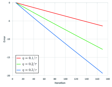
(a) $\tau=5$

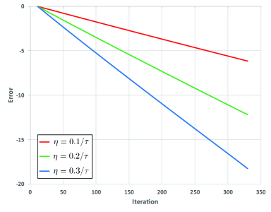
(b) $\tau=10$

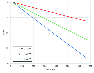
(c) $\tau=20$

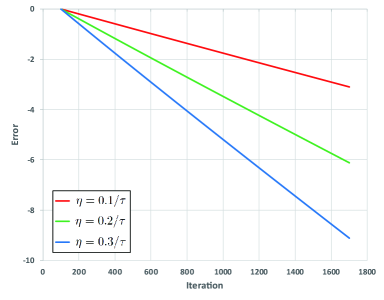
(d) $\tau=100$

Figure 1. Graphs of the log-scaled error $\mathcal{E}_{t}$ computed by the gradient descent with various delay $\tau=5$, $10$, $20$, $100$, regarding the least-squares regression problem.

On Figure 1, we depict some errors $\mathcal{E}_{t}$ variously simulated by setting $\eta=0.1/\tau$, $0.2/\tau$, $0.3/\tau$ for each delay $\tau$. In fact, the analyzed result (1.6) in Theorem 1.5 is rewritten as

$$\mathcal{E}_{t}=O(t).$$ (5.3)

Seeing all graphs in Figure 1, we observe that the numerical values of $\mathcal{E}_{t}$ have the linear property with respect to $t$ for any delay $\tau$. Compared with the number of iterations for each delay $\tau$, one additionally sees that the convergence of $\|x_{t}-x_{*}\|$ is faster as $\tau\rightarrow 0$. So, the reliability of (5.3) is obviously confirmed.

5.2. Logistic Classification

Consider the logistic classification problem: $\min_{x\in\mathbb{R}^{d}}f(x)$, where

$$f(x):=\frac{1}{m}\sum_{i=1}^{m}\ln\left(1+e^{-y_{i}A_{i}\cdot x}\right)+\frac{\mu}{2}\|x\|^{2},$$ (5.4)

where $A_{i}\in\mathbb{R}^{d}$ is a vector containing the $i$-th data point, and $y_{i}\in\{-1,1\}$ is the $i$-th associated class assignment. In this experiment, we try to choose $m=1,000$ data points: $500$ data points for the first class and $500$ data points for the second class. Each data point $A_{i}\sim\mathcal{N}(y_{i}{\bf 1},{\bf 1})$ is the Gaussian random variable of mean $y_{i}{\bf 1}$ and variance ${\bf 1}$, where

$$y_{i}=\left\{\begin{aligned} &1&&~{}~{}\mbox{ if }~{}1\leq i\leq 500,\\ &-1&&~{}~{}\mbox{ otherwise}.\end{aligned}\right.$$

Using the cost function $f(x)$ of (5.4) with $\mu=0.1$, we try to show the behavior of the error $\|x_{t}-x_{*}\|$ by simulating the concerned gradient descent scheme (1.1) with the delay $\tau=5$, $10$, $20$, $100$. As seen in the previous subsection, we set the initial point $x_{0}=0$ and the minimizer $x_{*}\in\mathbb{R}^{d}$ is approximately found by (1.1) within the tolerance ${\rm TOL}=10^{-10}$.

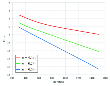
(a) $\tau=5$

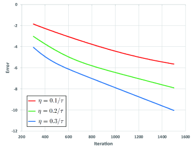
(b) $\tau=10$

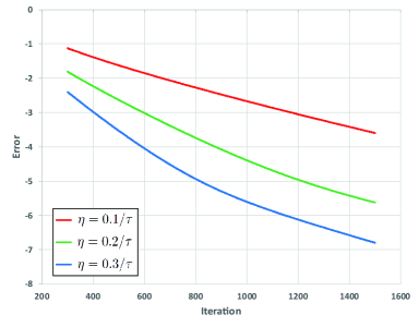
(c) $\tau=20$

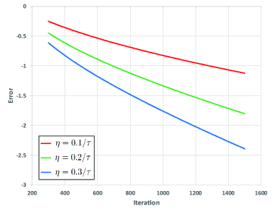
(d) $\tau=100$

Figure 2. Graphs of the log-scaled error $\mathcal{E}_{t}$ computed by the gradient descent with various delay $\tau=5$, $10$, $20$, $100$, regarding the logistic classification problem.

On Figure 2, we show the graphs of $\mathcal{E}_{t}$ obtained by the gradient descent scheme for each delay $\tau=5$, $10$, $20$, $100$ with various learning rate $\eta=0.1/\tau$, $0.2/\tau$, $0.3/\tau$. Seeing all graphs in Figure 2, the linear property of numerical values of $\mathcal{E}_{t}$ is still observed when the iteration $t$ is sufficiently large. This behavior also gives the reliability of the analyzed result (5.3).

5.3. Numerical example satisfying PL condition

In this subsection, we show the reliability of the analyzed result in Theorem 1.6. Consider the following cost function:

$$f(x)=\frac{1}{2}\|Ax-b\|^{2},$$ (5.5)

where $A\in\mathbb{R}^{m\times d}$ and $b\in\mathbb{R}^{m}$. If $d>m$, the cost $f(x)$ of (5.5) is not strongly convex, but it satisfies PL inequality provided that $AA^{T}\in\mathbb{R}^{m\times m}$ is a positive matrix. To construct the numerical example satisfying PL condition, we set $d=15$ and $m=6$, and moreover, all elements of $A$ and $b$ are independently generated by the Gaussian random variable of mean $0$ and variance $1$.

With the cost $f(x)$ given by (5.5), we try to simulate the gradient descent (1.1) with the delay $\tau=25$, based on the initial point $x_{0}=0$. We note that

$$\|\nabla f(y)-\nabla f(x)\|=\|A^{T}A(y-x)\|\leq L\|y-x\|,$$

where $L:=\|A^{T}A\|=\max\{\lambda>0:\lambda\mbox{ is an eigenvalue of }A^{T}A\}$. Choosing a sufficiently small number $\mu>0$ used in (1.7), the range of learning rate $\eta>0$ assumed in Theorem 1.6 becomes

$$\eta\leq\frac{D_{\tau}}{L\tau}\quad\textrm{with}\quad D_{\tau}:=\frac{2\tau}{\sqrt{1+4J_{\tau}\tau^{2}}+1}\simeq 0.8964.$$ (5.6)

For each iteration $t\geq\tau$, we define the log-scaled cost function error $e_{t}$ as

$$e_{t}:=\ln\left(\frac{f(x_{t})-f_{*}}{f(x_{\tau})-f_{*}}\right),$$

where $f_{*}$ denotes the minimal value of the given cost $f$, i.e., $f_{*}=f(x_{*})$. Actually, the minimizer $x_{*}\in\mathbb{R}^{d}$ can be obtained by $x_{*}=A^{+}b$, where $A^{+}$ is the pseudo-inverse of $A$.

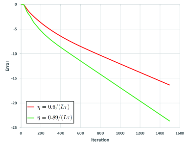
(a) $\eta=0.6/(L\tau)$, $0.89/(L\tau)$

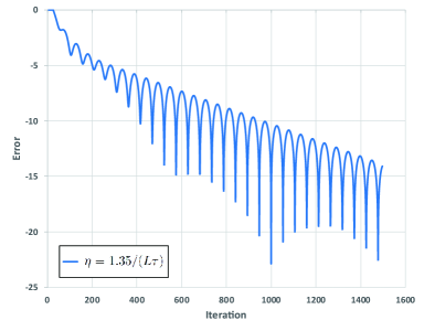
(b) $\eta=1.35/(L\tau)$

Figure 3. Graphs of the log-scaled cost error $e_{t}$ for the cost function $f(x)=2^{-1}\|Ax-b\|^{2}$, computed by the gradient descent with the delay $\tau=25$.

On Figure 3, we present the graphs of $e_{t}$ with respect to the iteration $t$ for some learning rates such as $\eta=0.6/(L\tau)$, $0.89/(L\tau)$, $1.35/(L\tau)$. We remark that the assumption (5.6) is satisfied in two cases: $\eta=0.6/(L\tau)$ and $\eta=0.89/(L\tau)$ but it is not satisfied in other case: $\eta=1.35/(L\tau)$. Seeing the graphs of Figure 3(a), it is observed that each error $e_{t}$ for $\eta=0.6/(L\tau)$ and $0.89/(L\tau)$ monotonically decays with linear rate, which is equivalent to the analyzed result (1.9) in Theorem 1.6. On the other hand, the oscillation of $e_{t}$ in the case of $\eta=1.3/(L\tau)$ can be found on Figure 3(b), that is, the error $e_{t}$ is not monotonically decreasing. So, this implies that the range of $\eta$ in the assuption of Theorem 1.6 may not be extended.

Conclusion

This paper establishes the linear convergence estimate for the gradient descent involving the delay, when the given cost function has the strongly convexity and $L$-smoothness. In addition, we give the analysis of linear convergence for the cost function error under the Polyak-Łojasiewicz condition and confirm its analyzed result by numerical experiment. In future works, we will thus extend our results to the related problems such as the online gradient descent with delay and the asynchronous stochastic gradient descent, and furthermore we will show that the analysis framework of this paper can be applicable in several ways.

References

- [1] A. Agarwal and J. C. Duchi, Distributed delayed stochastic optimization, Advances in Neural Information Processing Systems 24, 873-881, 2011.
- [2] Y. Arjevani, O. Shamir and N. Srebro, A tight convergence analysis for stochastic gradient descent with delayed updates, Proceedings of Machine Learning Research 117, 111-132, 2020.
- [3] S. Bubeck, Convex optimization: Algorithms and complexity, Foundations and Trends in Machine Learning 8, 231-357, 2015.
- [4] X. Cao and T. Başar, Decentralized online convex optimization with feedback delays, IEEE Transactions on Automatic Control 67(6), 2889-2904, 2022.
- [5] P. Joulani, A. Gyorgy and C. Szepesvári, Online learning under delayed feedback, Proceedings of Machine Learning Research 28(3), 1453-1461, 2013.
- [6] A. Koloskova, S. U. Stich and M. Jaggi, Sharper convergence guarantees for asynchronous SGD for distributed and federated learning, Advances in Neural Information Processing Systems 35, 17202-17215, 2022.
- [7] J. Langford, A. J. Smola and M. Zinkevich, Slow learners are fast, Advances in Neural Information Processing Systems 22, 2331-2339, 2009.
- [8] P. Liu, K. Lu, F. Xiao, B. Wei and Y. Zheng, Online distributed learning for aggregative games with feedback delays, IEEE Transactions on Automatic Control, 1-8, 2023.
- [9] K. Quanrud and D. Khashabi, Online learning with adversarial delays, Advances in Neural Information Processing Systems 28, 1270-1278, 2015.
- [10] K. Scaman, F. Bach, S. Bubeck, Y. T. Lee and L. Massoulié, Optimal algorithms for smooth and strongly convex distributed optimization in networks, Proceedings of Machine Learning Research 70, 3027-3036, 2017.
- [11] S. U. Stich and S. P. Karimireddy, The error-feedback framework: better rates for SGD with delayed gradients and compressed updates, The Journal of Machine Learning Research 21(1), 9613-9648, 2020.
- [12] S. Sra, A. W. Yu, M. Li and A. J. Smola, AdaDelay: Delay adaptive distributed stochastic convex optimization, Proceedings of Machine Learning Research 51, 957-965, 2016.
- [13] O. Shamir and L. Szlak, Online learning with local permutations and delayed feedback, Proceedings of Machine Learning Research 70, 3086-3094, 2017.
- [14] B. Sirb and X. Ye, Decentralized consensus algorithm with delayed and stochastic gradients, SIAM Journal on Optimization 28(2), 1232-1254, 2018.
- [15] C. Wang and S. Xu, Distributed online constrained optimization with feedback delays, IEEE Transactions on Neural Networks and Learning Systems, 1-13, 2022.
- [16] Y. Wan, W.-W. Tu and L. Zhang, Online strongly convex optimization with unknown delays, Machine Learning 111, 871-893, 2022.
- [17] M. Xiong, B. Zhang, D. Yuan, Y. Zhang and J. Chen, Event-triggered distributed online convex optimization with delayed bandit feedback, Applied Mathematics and Computation 445, 127865, 2023.