Effects of Quasiparticle-Vibration Coupling on Gamow-Teller Strength and $\beta$ Decay with the Skyrme Proton-Neutron Finite-Amplitude Method

Abstract

We adapt the proton-neutron finite-amplitude method, which in its original form is an efficient implementation of the Skyrme quasiparticle random phase approximation, to include the coupling of quasiparticles to like-particle phonons. The approach allows us to add beyond-QRPA correlations to computations of Gamow-Teller strength and $\beta$-decay rates in deformed nuclei for the first time. We test the approach in several deformed isotopes for which measured strength distributions are available. The additional correlations dramatically improve agreement with the data, and will lead to improved global $\beta$-decay rates.

I Introduction

The r process, which is responsible for synthesizing many of the heavy elements, is not fully understood Kajino et al. (2019). It is thought at present to occur primarily in neutron-star mergers, but may also take place in supernovae. To pin down the conditions under which rapid neutron capture and $\beta$ decay can lead to observed isotopic abundances, we need to understand the properties of nuclei that are too neutron-rich to be made in laboratories. Among the most important properties are $\beta$-decay rates.

Computing these rates in all neutron-rich isotopes is a difficult undertaking. Though ab initio methods for solving the nuclear many-body problem have made great strides Hergert (2020); Hagen et al. (2014); Navrátil et al. (2016); Lynn et al. (2019), they have not yet been extended to heavy nuclei far from closed shells. The best approach for now is energy-density-functional theory, in particular its version of linear response, which relates density oscillations to transition rates. References Mustonen and Engel (2016); Shafer et al. (2016); Ney et al. (2020); Marketin et al. (2016) have applied the charge-changing version of the Skyrme or relativistic quasiparticle random-phase approximation (QRPA) to produce tables of $\beta$-decay rates in thousands of isotopes. The method can be used either to compute transition rates directly through the diagonalization of a QRPA Hamiltonian matrix, or to extract the rates from response functions. The Hamiltonian matrix is so time-consuming to build, however, that the matrix approach in Ref. Marketin et al. (2016) required the assumption of spherical symmetry to obtain the thousands of rates needed for simulating nucleosynthesis.

With the advent of the finite amplitude method (FAM) Nakatsukasa et al. (2007); Avogadro and Nakatsukasa (2011) for computing QRPA linear response, calculations of strength distributions in deformed isotopes Stoitsov et al. (2011); Kortelainen et al. (2015); Hinohara et al. (2013) became straightforward. The global tables in Refs. Mustonen and Engel (2016); Ney et al. (2020) were obtained with the charge-changing version of this approach, called the proton-neutron FAM (pnFAM) Mustonen et al. (2014), and the assumption only of axial symmetry. The QRPA within density-functional theory has limitations, however, no matter how it is formulated. A linear response produced by oscillations of a mean-field is at best an adiabatic approximation, correct only at an oscillation frequency of zero, even if the time-independent functional on which the response is based is exact (which it never is). One can obtain a more realistic frequency-dependent response by coupling the quantized oscillations — phonons — to the quasiparticles that compose the phonons, or to other phonons. The first option, when developed systematically, leads in lowest order to the time-blocking approximation Kamerdzhiev et al. (1997); Litvinova et al. (2007, 2009); Tselyaev et al. (2016), which is equivalent to an density-functional version of what is called the “quasiparticle-vibration-coupling” model Colò et al. (1994); Li et al. (2022). Within Skyrme density-functional theory, this approximation has been used in a limited number of spherical nuclei to compute Gamow-Teller strength distributions Niu et al. (2016) and $\beta$-decay rates Niu et al. (2018). The phonons are like-particle excitations that are emitted and reabsorbed by the proton and neutron quasiparticles that underlie the excitations of the charge-changing QRPA. To make the picture produce the correct zero-frequency response, which is determined completely by the static Skyrme functional, one can employ the subtraction procedure first proposed in Ref. Tselyaev (2013).

The coupling of quasiparticles to phonons significantly improves agreement with data in spherical nuclei. One would like to use the method in global calculations of $\beta$-decay rates but faces the same problem encountered by the QRPA itself a few years ago: the usual implementation is through a Hamiltonian matrix, which is too time-consuming to construct when spherical symmetry cannot be exploited. Because the vast majority of nuclei are deformed, we thus need a different formalism. An extension of the pnFAM is the obvious choice. A formalism for the extension of the like-particle FAM with relativistic density functionals was developed, though not applied, in Refs. Zhang et al. (2022); Litvinova and Zhang (2022). Here we both show how to extend the pnFAM to include the coupling of quasiparticles to like-particle phonons and use the extension to compute Gamow-Teller distributions in several deformed isotopes, finding the agreement with experiment to be dramatically better than in the original pnFAM.

Treating $\beta$-decay in our new approach is a separate task because its rates are sensitive to small amounts of low-lying Gamow-Teller strength, which the Skyrme functionals that we have used in the past were adjusted to reproduce within the ordinary pnFAM. The parameters of the functionals must thus be refit before an improved table of rates can be created. We can, of course, demonstrate the effects of coupling quasiparticles to phonons on a few representative $\beta$-decay rates without refitting, and we do that here. The global application of the approach faces an additional obstacle, however: to obtain the interaction between quasiparticles and phonons, we apply the like-particle FAM in a way that will be hard to automate for use in the thousands of isotopes for which we need $\beta$-decay rates. Towards the end of this paper, we discuss relatively straightforward steps that will remedy the problem, deferring their implementation and the Skyrme-parameter refitting to the future.

The rest of the paper is structured as follows: Section II presents our method for adding the coupling of quasiparticles and phonons to the pnFAM and discusses subtleties that arise in deformed nuclei. Section III presents Gamow-Teller distributions in ⁷⁶Ge, ⁸²Se, and ¹⁵⁰Nd, and compares them with experimental data from charge-exchange reactions. Section IV presents $\beta$-decay rates in 12 deformed isotopes, showing that the new physics usually increases those rates. Section V contains a roadmap of sorts for the computation of $\beta$-decay rates in all unstable nuclei, a discussion of the explicit treatment of correlations within a density-functional framework, and a conclusion.

II Formalism

Our goal is to compute the strength distribution produced by a charge-changing operator $F$:

$$F=\sum_{pn}f_{pn}a^{\dagger}_{p}a_{n}\,,$$ (1)

where the coefficients $f_{pn}$ are arbitrary. The strength distribution can be written in the form

$$\frac{dB(F,\omega)}{d\omega}=-\frac{1}{\pi}\operatorname{Im}S_{F}(\omega)\,,$$ (2)

where $\omega$ is the frequency with which $F$ perturbs the nucleus (or equivalently, the amount of energy it supplies) and the “response function” $S_{F}(\omega)$ is

$$S_{F}(\omega)=-\sum_{M}\left(\frac{|\langle M|F|0\rangle|^{2}}{\Omega_{M}-\omega}-\frac{|\langle M|F^{{\dagger}}|0\rangle|^{2}}{\Omega_{M}+\omega}\right)\,.$$ (3)

Here $\ket{0}$ is the ground state of the initial nucleus and the $\ket{M}$’s are states in the final nuclei populated by single-charge-exchange processes with energies $\Omega_{M}$ above the energy of $\ket{0}$. The perturbing frequency/energy $\omega$ is a complex number a distance $\Delta$ above the real axis. Though $\Delta$ is supposed to be taken to zero at the end of any calculation, non-zero values supply widths to peaks that mock up effects of the continuum (which our calculations neglect).

After an HFB transformation, without proton-neutron mixing, the operator $F$ can be written as

$$F=\sum_{\pi\nu}\left(F^{20}_{\pi\nu}\alpha^{\dagger}_{\pi}\alpha^{\dagger}_{\nu}+F^{02}_{\pi\nu}\alpha_{\nu}\alpha_{\pi}+F^{11}_{\pi\nu}\alpha^{\dagger}_{\pi}\alpha_{\nu}+F^{11}_{\nu\pi}\alpha^{\dagger}_{\nu}\alpha_{\pi}\right)\,,$$ (4)

where the Greek letters $\pi$ and $\nu$ label proton and neutron quasiparticle orbitals, and $\alpha^{\dagger}$ and $\alpha$ represent operators that create and annihilate quasiparticles. The $F^{ij}_{\pi\nu}$ in Eq. (4) depend on the $f$’s in Eq. (1) and the HFB matrices $U$ and $V$ Ring and Schuck (2004) that specify the transformation from particles to quasiparticles. In the pnFAM, the response function can be written in the form

$$S_{F}(\omega) =\sum_{\pi\nu}\left[F_{\pi\nu}^{20*}X_{\pi\nu}(\omega)+F_{\pi\nu}^{02*}Y_{\pi\nu}(\omega)\right]\,,$$ (5)

where the $X$’s and $Y$’s are the fluctuation amplitudes in density-matrix elements induced by the action of $F$, applied at frequency $\omega$. The pnFAM equations for these amplitudes are Mustonen et al. (2014)

$$X_{\pi\nu}(\omega) =-\frac{\delta H_{\pi\nu}^{20}(\omega)+F_{\pi\nu}^{20}(\omega)}{\varepsilon_{\pi}+\varepsilon_{v}-\omega}$$ (6)

$$Y_{\pi\nu}(\omega) =-\frac{\delta H_{\pi\nu}^{02}(\omega)+F_{\pi\nu}^{02}(\omega)}{\varepsilon_{\pi}+\varepsilon_{v}+\omega}\,.$$

Here the $\varepsilon$’s are quasiparticle energies and $\delta H_{\pi\nu}^{20}$ and $\delta H_{\pi\nu}^{02}$ are the pieces of the fluctuating generalized HFB mean-field Hamiltonian that multiply pairs of quasiparticle creation and annihilation operators in the same way as do $F^{20}_{\pi\nu}$ and $F^{02}_{\pi\nu}$ in Eq. (4). Because $\delta H^{20}$ and $\delta H^{02}$ depend on the $X$’s and $Y$’s, Eqs. (6) are most easily solved through iteration.

In the QRPA, the states $\ket{M}$ are simple two-quasiparticle and two-quasihole excitations of the ground state $\ket{0}$. We want to make these simple states more realistic by allowing them to mix with states that include coherent like-particle excitations. The most straightforward way of doing that is to allow the emission and re-absorption of like-particle QRPA phonons by one of the quasiparticles in the two-quasiparticle excitation of $\ket{0}$, or the exchange of such a phonon between the two. When only one phonon is allowed to exist at a time within a time-ordered picture for the two-quasiparticle propagator, we end up with the quasiparticle-vibration coupling model Niu et al. (2016) or, equivalently, the time-blocking approximation Litvinova et al. (2007); Tselyaev et al. (2016).

The modifications to the FAM equations induced by the quasiparticle-phonon coupling can be derived in a number of ways. One can, for example, follow the equations of motion method for charge-changing excitations, for example, using the ansatz

$$\ket{M}=Q_{M}^{\dagger}\ket{0}\,,$$ (7)

with

$$Q^{\dagger}_{M} =\sum_{\pi\nu}\big{(}X^{M}_{\pi\nu}\alpha^{\dagger}_{\pi}\alpha^{\dagger}_{\nu}-Y^{M}_{\pi\nu}\alpha_{\nu}\alpha_{\pi}$$ (8)

$$\qquad+\sum_{N}\tilde{X}^{M}_{\pi\nu N}\alpha^{\dagger}_{\pi}\alpha^{\dagger}_{\nu}\mathcal{Q}^{\dagger}_{N}-\tilde{Y}^{M}_{\pi\nu N}\mathcal{Q}_{N}\alpha_{\nu}\alpha_{\pi}\big{)}\,.$$

Here $\mathcal{Q}^{\dagger}_{N}$ creates the $N^{\text{th}}$ like-particle phonon (with non-negative energy) in the usual like-particle QRPA, the $X$’s and $Y$’s are now charge-changing QRPA-level amplitudes, and the $\tilde{X}$’s and $\tilde{Y}$’s are beyond-QRPA amplitudes that specify the ways in which quasiparticles couple to phonons. One might also include terms in which pairs of like quasiparticles couple to charge-changing phonons, but those are less important Robin and Litvinova (2018) and we neglect them here.

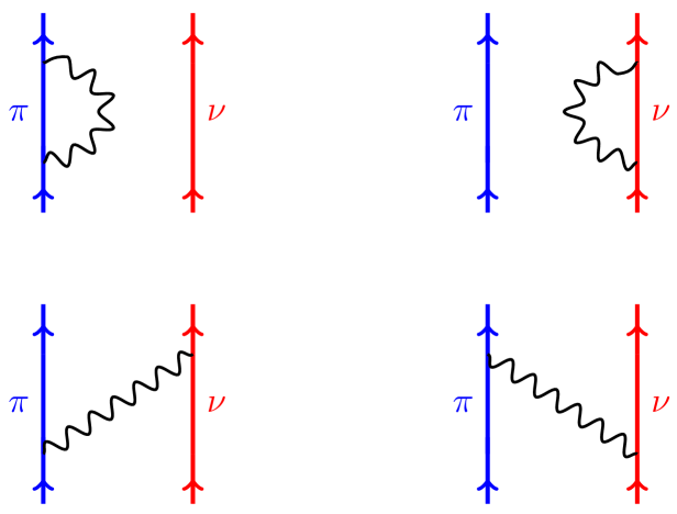
Figure 1: Diagrams illustrating the four contributions to the “spreading matrix” $W$ in Eq. (12). Blue lines represent protons and red lines neutrons. Black squiggly lines represent phonons, either emitted and re-absorbed by a single nucleon or exchanged between nucleons.

When the complicated amplitudes $\tilde{X}$ and $\tilde{Y}$ are eliminated in the usual way in favor of a propagator in the space of complicated excitations, one finds, instead of Eq. (6), relations that we refer to as the pnFAM* equations:

$$X_{\pi\nu}(\omega) =-\frac{\delta H_{\pi\nu}^{20}+\left[\tilde{W}(\omega)X(\omega)\right]_{\pi\nu}+F_{\pi\nu}^{20}}{\varepsilon_{\pi}+\varepsilon_{\nu}-\omega}$$ (9)

$$Y_{\pi\nu}(\omega) =-\frac{\delta H_{\pi\nu}^{02}+\left[\tilde{W}^{*}(-\omega)Y(\omega)\right]_{\pi\nu}+F_{\pi\nu}^{02}}{\varepsilon_{\pi}+\varepsilon_{\nu}+\omega}\,,$$

where

$$\tilde{W}(\omega)=W(\omega)-W(0)\,,$$ (10)

and

$$\left[\tilde{W}(\omega)X(\omega)\right]_{\pi\nu} =\sum_{\pi^{\prime}\nu^{\prime}}\tilde{W}_{\pi\nu,\pi^{\prime}\nu^{\prime}}(\omega)X_{\pi^{\prime}\nu^{\prime}}(\omega)$$ (11)

$$\left[\tilde{W}^{*}(-\omega)Y(\omega)\right]_{\pi\nu} =\sum_{\pi^{\prime}\nu^{\prime}}\tilde{W}_{\pi\nu,\pi^{\prime}\nu^{\prime}}^{*}(-\omega)Y_{\pi^{\prime}\nu^{\prime}}(\omega)\,,$$

The matrix $W$, which includes a phonon-loop correction to single-quasiparticle energies and a phonon-exchange interaction (see Fig. 1) is given by

$$W {}_{\pi\nu,\pi^{\prime}\nu^{\prime}}(\omega)=\sum_{N}\Bigg{\{}\sum_{\pi_{1}}\left\langle\pi|H|\pi_{1},N\right\rangle\frac{1}{\omega-\left[\omega_{N}+\left(\varepsilon_{\pi_{1}}+\varepsilon_{\nu}\right)\right]}\left\langle\pi^{\prime}|H|\pi_{1},N\right\rangle^{*}\delta_{\nu^{\prime}\nu}$$ (12)

$$\qquad\qquad\qquad\qquad\qquad+\sum_{\nu_{1}}\left\langle\nu|H|\nu_{1},N\right\rangle\frac{1}{\omega-\left[\omega_{N}+\left(\varepsilon_{\pi}+\varepsilon_{\nu_{1}}\right)\right]}\left\langle\nu^{\prime}|H|\nu_{1},N\right\rangle^{*}\delta_{\pi^{\prime}\pi}$$

$$\qquad\qquad+\left\langle\pi|H|\pi^{\prime},N\right\rangle\frac{1}{\omega-\left[\omega_{N}+\left(\varepsilon_{\pi^{\prime}}+\varepsilon_{\nu}\right)\right]}\left\langle\nu^{\prime}|H|\nu,N\right\rangle^{*}+\left\langle\nu|H|\nu^{\prime},N\right\rangle\frac{1}{\omega-\left[\omega_{N}+\left(\varepsilon_{\pi}+\varepsilon_{\nu^{\prime}}\right)\right]}\left\langle\pi^{\prime}|H|\pi,N\right\rangle^{*}\Bigg{\}}\,.$$

Here $\omega_{N}$ is the energy of the $N^{\text{th}}$ like particle phonon. Each of the four terms in Eq. (12) corresponds to one of the diagrams in Fig. 1. Using $\tilde{W}(\omega)$ instead of $W(\omega)$ in Eq. (9) implements the subtraction procedure Tselyaev (2013) that guarantees that the static response is the same as in the unmodified pnFAM Gambacurta et al. (2015).

Within the expression in Eq. (12) for $W$, which is sometimes called the “spreading matrix,” are quasiparticle-phonon vertices, matrix elements of the Hamiltonian with a single quasiparticle on one side and another quasiparticle of the same type plus a phonon on the other. The phonons can be excited by a like-particle one-body operator $G$:

$$G=\sum_{pp^{\prime}}G_{pp^{\prime}}a^{\dagger}_{p}a_{p^{\prime}}+\sum_{nn^{\prime}}G_{nn^{\prime}}a^{\dagger}_{n}a_{n^{\prime}}\,,$$ (13)

where $p,p^{\prime}$ label proton orbitals and $n,n^{\prime}$ label neutron orbitals. In like-particle linear-response theory, $G$ generates fluctuations $\delta H$ in the like-particle HFB Hamiltonian. The quasiparticle-phonon vertices can be related to $\delta H^{11}$, the coefficients of operators of the form $\alpha^{\dagger}_{\nu}\alpha_{\nu^{\prime}}$ and $\alpha^{\dagger}_{\pi}\alpha_{\pi^{\prime}}$ in the fluctuating like-particle HFB Hamiltonian, through a contour integral Hinohara et al. (2013) or, as Ref. Zhang et al. (2022) shows, through the relation

$$\braket{\beta}{H}{\beta_{1},N}=i\lim_{\Delta\to 0}\frac{\Delta}{\braket{N}{G}{0}}\delta H^{11}_{\beta\beta_{1}}(\Omega_{N}+i\Delta)\,.$$ (14)

Here $\beta$ and $\beta_{1}$ can represent either proton or neutron quasiparticle orbitals as long as they are of the same type, and $\braket{N}{G}{0}$ is the matrix element connecting the ground state with the $N^{\text{th}}$ phonon. In the like-particle FAM, this last quantity can be extracted up to an arbitrary and irrelevant phase from the like-particle response function $S_{G}$,

$$S_{G}(\omega)=-\sum_{N}\left(\frac{|\langle N|G|0\rangle|^{2}}{\omega_{N}-\omega}-\frac{|\langle N|G^{\dagger}|0\rangle|^{2}}{\omega_{N}+\omega}\right)\,,$$ (15)

as

$$\braket{N}{G}{0}=\lim_{\Delta\to 0}\sqrt{i\Delta S_{G}(\omega_{N}+i\Delta)}\,.$$ (16)

In this paper, in place of the generic charge-changing operator $F$ we will usually use the components of the Gamow-Teller operator,

$$F_{K}=\sum_{i}\sigma_{K}(i)\tau_{-}(i)\,,$$ (17)

where the sum is over nucleons, $K$ labels the projection of the angular momentum along the $z$ axis, and $\tau_{-}\equiv\frac{1}{2}(\tau_{x}-i\tau_{y})$ — note the non-standard normalization — turns neutron states into proton states while annihilating the latter. In place of $G$ we will use the multipole operators

$$G^{T=0}_{LK} =\sum_{i}r_{i}^{L}Y_{LK}(\theta_{i},\varphi_{i})$$ (18)

$$G^{T=1}_{LK} =\sum_{i}r_{i}^{L}Y_{LK}(\theta_{i},\varphi_{i})\tau_{z}(i)\,,$$

where $\tau_{z}$ is 1 for neutrons and $-1$ for protons. Here $L$ is any integer, $r$ is the radial coordinate, and $Y_{LK}$ is the spherical harmonic with angular momentum $L$ and $z$-projection $K$. For a given charge-changing projection $K$, like-particle phonons created by operators $G^{T}_{L,K^{\prime}}$ with any value of $K^{\prime}$ can play a role. To eliminate the spurious states corresponding to translation and rotation, we simply discard phonons with an energy less than 0.5 MeV.

III Gamow-Teller Strength Functions

The computation of strength functions proceeds as follows: First, we use the code HFBTHO Stoitsov et al. (2005, 2013) to solve the HFB equations for arbitrary Skyrme functionals. In the work here, we use a single-particle space consisting of 16 shells. With quasiparticle energies and wave functions in hand, we then run the like-particle FAM enough times to generate all states excited by the natural-parity operators in Eq. (18) with $L\leq 6$. (our code is not yet set up for the less-important unnatural-parity excitations). To isolate those states, in each multipole (specified by $L$ and $K$ in spherical nuclei, and parity and $K$ in deformed nuclei) we solve the FAM equations for 40 values of the excitation frequency $\omega$ between 0 and 20 MeV, with an imaginary component of 0.5 MeV, to identify the peaks in the strength function. For each such peak we run the FAM several times again, with the real part of $\omega$ at the energy of the peak and the imaginary part decreasing towards zero, and use Eq. (14) to compute the quasiparticle-phonon vertices.

The final step is to use Eq. (12) to construct the spreading matrix $W$ and solve the pnFAM* equations in Eq. (9). Rather than store the four-index matrix $W$, we store the simpler quasiparticle-phonon vertices and construct $W$ on the fly as needed. After obtaining $X_{\pi\nu}(\omega)$ and $Y_{\pi\nu}(\omega)$ for many values of $\omega$ near the real axis, we use Eqs. (2) and (5) to construct first the response and then the Gamow-Teller strength distribution.

In what follows, we display results for the strength distribution obtained with the Skyrme functional SGII Van Giai and Sagawa (1981a, b), which was designed for spin-isospin excitations, with the same effective interaction in the time-even and time-odd channels. The pairing is mixed surface-volume, with strengths of $-265.25$ MeV ​fm³ for neutrons and $-340.0625$ MeV ​fm³ for protons, and a pairing window cut off at 60 MeV. Distributions have been measured in several nuclei that can undergo $\beta\beta$ decay (to provide information that bears on the matrix elements that govern the two-neutrino and neutrinoless versions of that process), and we begin with the ⁸²Se. Our HFBTHO calculations predict the nucleus to have mild axially-symmetric deformation, with the quadrupole-deformation parameter,

$$\beta=\sqrt{\frac{\pi}{5}}\frac{Q_{2}}{R^{2}}\,,$$ (19)

given by $\beta=0.13$. Here $Q_{2}$ is the usual quadrupole moment and $R^{2}$ the mean-square nuclear radius.

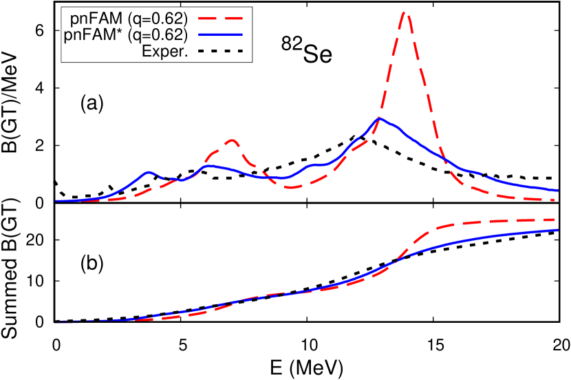
Figure 2: (a) Gamow-Teller strength distributions for the nucleus ⁸²Se. The red dashed and solid blue curves, representing results calculated with the pnFAM and pnFAM* (see text), have been scaled by 0.62. The black curve, from Ref. Madey et al. (1989) is experimental data. In obtaining each curve, we chose the imaginary part $\Delta$ of the perturbing frequency to be 0.5 MeV. (b) Integrated Gamow-Teller strength.

Figure 2 shows the distributions both of the strength itself and the summed strength, with each scaled by a factor of 0.62 that would correspond to an effective value for the axial-vector coupling constant $g_{A}$ of $1.0$ in $\beta$ decay calculations. The figure also displays the measured strength Madey et al. (1989), the overall normalization of which is highly uncertain. The most salient feature of the pnFAM* strength is that it is spread, and thus agrees much better with the experimental distribution. It is not very quenched, however, which is why we scale it; evidently the absence of multi-phonon emission and reabsorption in $W$ is responsible for the small quenching. (As in most extended QRPAs, the Ikeda sum rule is preserved, so that any quenching of low-energy strength implies a long tail at high energies, as in Ref. Gambacurta et al. (2020).) Both the spreading and lack of significant quenching with the coupling of quasiparticles to vibrations are consistent with results in spherical nuclei Niu et al. (2016); Gambacurta et al. (2020). But, in a promising sign for the ability of these calculations to improve on pnFAM calculations of $\beta$-decay rates, the figure shows the pnFAM* low-lying strength, by far the most important for $\beta$ decay, to be much closer to that of experiment.

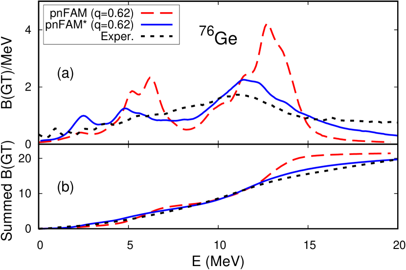
Figure 3: Same as in Fig. 2 but for ⁷⁶Ge.

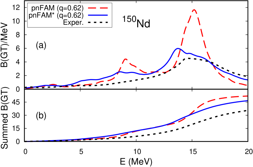
Figure 4: Same as in Fig. 2 but for ¹⁵⁰Nd, with the experimental data from Ref. Guess et al. (2011).

Figure 3 shows the same curves as Fig. 2 but for the nucleus ⁷⁶Ge. Recent work, both experimental Toh et al. (2013); Ayangeakaa et al. (2019) and theoretical Rodríguez (2017), suggests that this nucleus is triaxial, but we (are forced to) treat it as axially symmetric, with a deformation parameter from HFBTHO of $\beta=0.12$. The same features are apparent here as in Fig. 2.

Figure 4 shows the curves for the significantly heavier and more deformed nucleus ¹⁵⁰Nd, which in our calculations has $\beta=0.21$. Again, the pnFAM* improves agreement with experiment overall, but an even stronger quenching than the 0.62 we apply is called for.

The addition of the spreading matrix $W$ to the pnFAM slows the computation, both because of the time required to evaluate $W$ and because the values for $X_{\pi\nu}(\omega)$ and $Y_{\pi\nu}(\omega)$ in the iterative solution of Eqs. (9) converge more slowly than do those in Eqs. (6). To speed the computation, we would like to include as few like-particle phonons as possible in the spreading matrix in Eq. (12). But how do we decide which are the most important and how many do we include? These questions were addressed in spherical nuclei in Ref. Tselyaev et al. (2017). The authors showed that to evaluate the importance of the $N^{\text{th}}$ phonon one can reliably use the ratio of the expectation value $\braket{V}_{N}$ of the interaction in the phonon state to the phonon energy $\omega_{N}$:

$$v_{N}\equiv\frac{\braket{V}_{N}}{\omega_{N}}\,,$$ (20)

This measure, justified carefully in Ref. Tselyaev et al. (2017), reflects the perturbative phonon exchange, which accentuates the importance of low-energy phonons, and the relation between $\braket{V_{N}}$ and the quasiparticle-phonon vertices in Eq. (14). After some manipulation, $v_{N}$ can be written in the form

$$v_{N}=1-\frac{1}{\omega_{N}}\sum_{\alpha\beta}\left(\varepsilon_{\alpha}+\varepsilon_{\beta}\right)\left(\left|\mathcal{X}^{N}_{\alpha\beta}\right|^{2}+\left|\mathcal{Y}^{N}_{\alpha\beta}\right|^{2}\right)\,.$$ (21)

Here the $\mathcal{X}$’s and $\mathcal{Y}$’s are the like-particle QRPA analogs of pnQRPA $X$’s and $Y$’s in Eq. (8), and the indices $\alpha$ and $\beta$ run over all pairs in which both label protons or both label neutrons. Equations (24) in Ref. Hinohara et al. (2013) implies that we can extract the $\mathcal{X}$’s and $\mathcal{Y}$’s as the limits,

$$\mathcal{X}^{N}_{\alpha\beta} =-i\lim_{\Delta\to 0}\frac{\Delta}{\braket{N}{G}{0}}\mathcal{X}_{\alpha\beta}(\omega_{N}+i\Delta)$$ (22)

$$\mathcal{Y}^{N}_{\alpha\beta} =-i\lim_{\Delta\to 0}\frac{\Delta}{\braket{N}{G}{0}}\mathcal{Y}_{\alpha\beta}(\omega_{N}+i\Delta)\,.$$

Here $G$ is one of the multipole operators in Eq. (18) and the $\mathcal{X}_{\alpha\beta}(\omega)$ and $\mathcal{Y}_{\alpha\beta}(\omega)$ are the like-particle FAM amplitudes, i.e. the analogs of the pnFAM $X$’s and $Y$’s in Eq. (6).

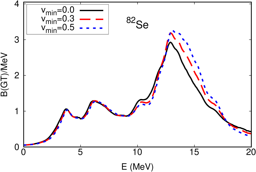
Figure 5: Gamow-Teller strength distribution in ⁸²Se obtained in the pnFAM*, with several values for the cutoff parameter $v_{\text{min}}$. The lower that quantity, the more phonons the calculation includes. As before, we include all natural-parity multipoles with $L\leq 6$.

Figure 5 shows the results in ⁸²Se of requiring that $|v_{N}|$ be larger than a critical value $v_{\text{min}}$ as that quantity decreases. At the smallest value, $v_{\text{min}}=0$, there is no truncation and the calculation includes all the 150 phonons corresponding to distinct maxima in the like-particle strength functions, when plotted with $\Delta=0.5$ MeV. At the values $v_{\text{min}}=0.3$, and $0.5$, the calculation includes 62 and 35 phonons, respectively. Although truncation has a noticeable effect in the giant Gamow-Teller resonance, even the most dramatic one does very little at low energies. That means that when calculating $\beta$ decay rates, we can expect to get away with relatively few phonons. The effects of truncation in ⁷⁶Ge and ¹⁵⁰Nd are similar.

To conclude this section, we look at the effects of limiting ourselves to like-particle excitation operators with $L\leq 6$ in Eq. (18). Figure 6 shows strength distributions in ⁸²Se for different values $L_{\text{max}}$ of the maximum angular momentum in the excitation operators. One can see that by $L_{\text{max}}=5$ the distribution has converged. The pattern is almost exactly the same in other two isotopes we examined earlier.

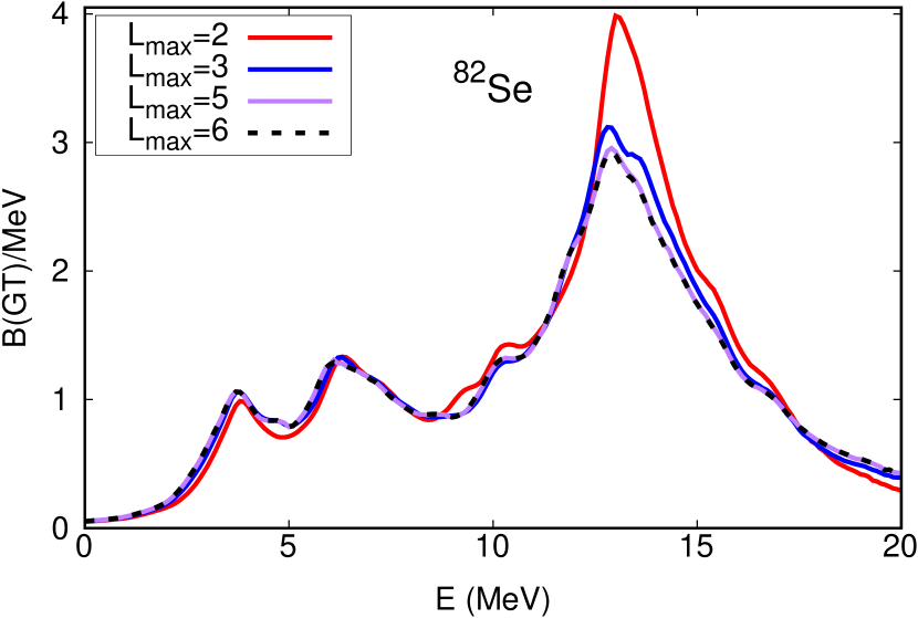
Figure 6: Gamow-Teller strength distribution in ⁸²Se obtained in the pnFAM*, with several values for the maximum angular momentum $L_{\text{max}}$ in states excited by the like-particle operators in Eq. (18). No other cutoffs are imposed, i.e. $v_{\text{min}}=0$.

IV $\beta$-decay rates

As we’ve noted, $\beta$-decay rates depend sensitively on details of the low-lying parts of strength distributions. Unlike gross features such as giant resonances, low-lying strength is strongly affected by the isoscalar pairing interaction, the coefficient of which was fit in global Skyrme-QRPA calculations of $\beta$ decay Mustonen and Engel (2016); Ney et al. (2020). As we have seen, allowing quasiparticles to couple to phonons also alters low-lying strength. So that we do not confuse the effects, we continue to work with SGII, without isoscalar pairing.

Table 1: Deformation parameter, experimental half-life in seconds, pnFAM half-life with the Skyrme functional SGII, pnFAM* half-life with the same functional, and pnFAM* half-life when phonons with $v_{N}<0.3$ are excluded, for 11 deformed isotopes.

Isotope	$\beta$	$t_{1/2}^{\text{Exp.}}$(s)	$t_{1/2}^{\text{pnFAM}}$(s)	$t_{1/2}^{\text{pnFAM*}}$(s)	$t_{1/2}^{\prime\text{\ pnFAM*}}$(s)
78Zn	0.12	1.47	408	3.77	4.80
168Gd	0.31	3.03	381	37.1	39.7
152Ce	0.29	1.40	93.1	19.0	20.3
156Nd	0.32	5.49	470	53.5	59.2
164Sm	0.33	1.42	142	17.2	18.5
154Ce	0.30	0.30	19.2	7.26	7.89
112Mo	$-0.18$	0.15	1.92	2.47	2.31
94Kr	$-0.22$	0.21	1.48	3.23	3.01
112Ru	$-0.21$	1.75	93	27.0	31.0
106Mo	$-0.20$	8.73	62.8	38.0	49.6
96Sr	$-0.21$	1.07	23.8	20.0	25.9

Table 1 shows the effects of the quasiparticle-phonon coupling on decay rates in 11 representative heavy nuclei. Six of the 11 are prolate and five are oblate (though data in ¹⁰⁶Mo, which we find to be oblate, may be more consistent with prolate deformation Ha et al. (2020)). In all the isotopes, the pnFAM without any modification over-predicts the lifetimes by placing too little strength at low energies. In the prolate cases, the quasiparticle-phonon coupling always reduces the lifetime, often dramatically, and always improves the agreement with experiment. Though the effect is smaller, the agreement is usually better in the oblate isotopes as well. In two of them, however, the coupling actually increases the lifetime slightly, making the agreement with experiment a little worse. Because most of the allowed rates increase in the pnFAM*, the forbidden contributions to the decay, which increase less, are a smaller percentage of the total rate than in the pnFAM itself.

In prior global QRPA calculations, isoscalar pairing was used to increase the strength below the $\beta$-decay $Q$ value, decreasing predicted lifetimes so that on average they were correct. Many were significantly too small, however, and many others significantly too large, in spite of the isoscalar pairing. With the coupling of quasiparticles to phonons also increasing lifetimes (usually), in a way that is more natural, isoscalar pairing can be weakened. Though we don’t know for sure that the fluctuations in computed rates will be smaller than before, work in spherical nuclei Niu et al. (2018) suggests that they will.

V Discussion

Our method for including the coupling of quasiparticles to phonons is much more efficient than the extension of the matrix QRPA. It is not yet efficient enough, however, to allow us to apply it to all of the approximately 4000 neutron-rich isotopes. At present, we extract the quasiparticle-phonon coupling by first computing like-particle strength functions at many values of $\omega$ and in many channels, identifying peaks, and employing Eqs. (14) and (16) for each one. How might we get the same information more efficiently?

One advantage of the traditional matrix QRPA is that it directly produces the transition amplitudes $\mathcal{X}^{N}_{\alpha\beta}$ and $\mathcal{Y}^{N}_{\alpha\beta}$ [see Eq. (22)], which in turn determine $\braket{\beta}{H}{\beta_{1},N}$ and therefore $W_{\pi\nu,\pi^{\prime}\nu^{\prime}}(\omega)$ in a straightforward algebraic way. The chief disadvantage is the long time it takes to construct the many elements of the QRPA Hamiltonian matrix. The FAM can actually be used to construct the matrix much faster Avogadro and Nakatsukasa (2013), and a starting point for future work is to build and diagonalize the matrix, use the results and Eq. (21) to select the most important phonons, and then construct $W$. And we can do even better by employing a Lanczos-like approach to produce only the most important parts of the matrix. Ref. Toivanen et al. (2010) applies the Arnoldi algorithm in concert with a FAM-like procedure to obtain matrices with dimensions of order $100\times 100$ that, when diagonalized, reproduce strength distributions accurately. Another promising option is to use expand the QRPA $\mathcal{X}$’s and $\mathcal{Y}$’s in terms of FAM amplitudes at values of $\omega$ far from the real axis. This approach, which we will present in a separate paper Hinohara et al. , is analogous to the eigenvalue continuation introduced in Ref. Frame et al. (2018).

Once we have a faster procedure, we will be able use the pnFAM* to refit the parameters of the time-odd part of any Skyrme functional to a set of selected $\beta$-decay rates, charge-changing resonance energies, etc., as was done with the pnFAM itself in Ref. Mustonen and Engel (2016). We can also include in the fit the parameters multiplying chiral two-body weak-current operators, the infrastructure for which was presented in Ref. Ney et al. (2022). The result should be much better predictions for $r$-process simulations.

This plan raises the question of what it means to extend density-functional theory beyond the QRPA, i.e. beyond a time-dependent mean-field ansatz. Does it make sense to use a density-dependent “Hamiltonian” in conjunction with beyond-mean-field correlations? Aren’t the correlations already implicit in the functional itself? We need not answer these questions carefully to be confident that including more correlations is worthwhile. Doing so pushes our method in the direction of an ab initio solution of the Schrödinger equation. Double counting of correlations can be removed through parameter refitting. The more correct physics we include by extending our many-body methods, the less we burden the functional with mocking that physics up. An exact many-body method would be appropriate in conjunction with a functional that corresponds simply to the mean-field expectation value of an ab initio Hamiltonian. Our long term goal is to push nuclear density-functional theory as close to that point as possible. The improved description of charge-changing processes presented here is a good start.

References

- Kajino et al. (2019) T. Kajino, W. Aoki, A. Balantekin, R. Diehl, M. Famiano, and G. Mathews, Progress in Particle and Nuclear Physics 107, 109 (2019).
- Hergert (2020) H. Hergert, Frontiers in Physics 8, article 379 (2020).
- Hagen et al. (2014) G. Hagen, T. Papenbrock, M. Hjorth-Jensen, and D. J. Dean, Reports on Progress in Physics 77, 096302 (2014).
- Navrátil et al. (2016) P. Navrátil, S. Quaglioni, G. Hupin, C. Romero-Redondo, and A. Calci, Physica Scripta 91, 053002 (2016).
- Lynn et al. (2019) J. Lynn, I. Tews, S. Gandolfi, and A. Lovato, Annual Review of Nuclear and Particle Science 69, 279 (2019), https://doi.org/10.1146/annurev-nucl-101918-023600 .
- Mustonen and Engel (2016) M. T. Mustonen and J. Engel, Phys. Rev. C 93, 014304 (2016).
- Shafer et al. (2016) T. Shafer, J. Engel, C. Fröhlich, G. C. McLaughlin, M. Mumpower, and R. Surman, Phys. Rev. C94, 055802 (2016).
- Ney et al. (2020) E. M. Ney, J. Engel, T. Li, and N. Schunck, Phys. Rev. C 102, 034326 (2020).
- Marketin et al. (2016) T. Marketin, L. Huther, and G. Martinez-Pinedo, Phys. Rev. C93, 025805 (2016).
- Nakatsukasa et al. (2007) T. Nakatsukasa, T. Inakura, and K. Yabana, Phys. Rev. C 76, 024318 (2007).
- Avogadro and Nakatsukasa (2011) P. Avogadro and T. Nakatsukasa, Phys. Rev. C 84, 014314 (2011).
- Stoitsov et al. (2011) M. Stoitsov, M. Kortelainen, T. Nakatsukasa, C. Losa, and W. Nazarewicz, Phys. Rev. C 84, 041305(R) (2011).
- Kortelainen et al. (2015) M. Kortelainen, N. Hinohara, and W. Nazarewicz, Phys. Rev. C 92, 051302(R) (2015).
- Hinohara et al. (2013) N. Hinohara, M. Kortelainen, and W. Nazarewicz, Phys. Rev. C 87, 064309 (2013).
- Mustonen et al. (2014) M. T. Mustonen, T. Shafer, Z. Zenginerler, and J. Engel, Phys. Rev. C 90, 024308 (2014).
- Kamerdzhiev et al. (1997) S. P. Kamerdzhiev, G. Y. Tertychnyi, and V. I. Tselyaev, Physics of Particles and Nuclei 28, 134 (1997).
- Litvinova et al. (2007) E. Litvinova, P. Ring, and V. Tselyaev, Phys. Rev. C 75, 064308 (2007).
- Litvinova et al. (2009) E. Litvinova, P. Ring, V. Tselyaev, and K. Langanke, Phys. Rev. C 79, 054312 (2009).
- Tselyaev et al. (2016) V. Tselyaev, N. Lyutorovich, J. Speth, S. Krewald, and P.-G. Reinhard, Phys. Rev. C 94, 034306 (2016).
- Colò et al. (1994) G. Colò, N. Van Giai, P. F. Bortignon, and R. A. Broglia, Phys. Rev. C 50, 1496 (1994).
- Li et al. (2022) Z. Z. Li, Y. F. Niu, and G. Colò, (2022), 10.48550/ARXIV.2211.01264.
- Niu et al. (2016) Y. F. Niu, G. Colò, E. Vigezzi, C. L. Bai, and H. Sagawa, Phys. Rev. C 94, 064328 (2016).
- Niu et al. (2018) Y. F. Niu, Z. M. Niu, G. Colò, and E. Vigezzi, Physics Letters, Section B: Nuclear, Elementary Particle and High-Energy Physics 780, 325 (2018).
- Tselyaev (2013) V. I. Tselyaev, Phys. Rev. C 88, 054301 (2013).
- Zhang et al. (2022) Y. Zhang, A. Bjelčić, T. Nikšić, E. Litvinova, P. Ring, and P. Schuck, Phys. Rev. C 105, 044326 (2022).
- Litvinova and Zhang (2022) E. Litvinova and Y. Zhang, Phys. Rev. C 106, 064316 (2022).
- Ring and Schuck (2004) P. Ring and P. Schuck, The Nuclear Many-Body Problem, Texts and Monographs in Physics (Springer, 2004).
- Robin and Litvinova (2018) C. Robin and E. Litvinova, Phys. Rev. C 98, 051301(R) (2018).
- Gambacurta et al. (2015) D. Gambacurta, M. Grasso, and J. Engel, Phys. Rev. C 92, 034303 (2015).
- Stoitsov et al. (2005) M. Stoitsov, J. Dobaczewski, W. Nazarewicz, and P. Ring, Computer Physics Communications 167, 43 (2005).
- Stoitsov et al. (2013) M. Stoitsov, N. Schunck, M. Kortelainen, N. Michel, H. Nam, E. Olsen, J. Sarich, and S. Wild, Comput. Phys. Commun. 184, 1592 (2013).
- Van Giai and Sagawa (1981a) N. Van Giai and H. Sagawa, Physics Letters B 106, 379 (1981a).
- Van Giai and Sagawa (1981b) N. Van Giai and H. Sagawa, Nuclear Physics A 371, 1 (1981b).
- Madey et al. (1989) R. Madey, B. S. Flanders, B. D. Anderson, A. R. Baldwin, J. W. Watson, S. M. Austin, C. C. Foster, H. V. Klapdor, and K. Grotz, Phys. Rev. C 40, 540 (1989).
- Gambacurta et al. (2020) D. Gambacurta, M. Grasso, and J. Engel, Phys. Rev. Lett. 125, 212501 (2020).
- Guess et al. (2011) C. J. Guess, T. Adachi, H. Akimune, A. Algora, S. M. Austin, D. Bazin, B. A. Brown, C. Caesar, J. M. Deaven, H. Ejiri, E. Estevez, D. Fang, A. Faessler, D. Frekers, H. Fujita, Y. Fujita, M. Fujiwara, G. F. Grinyer, M. N. Harakeh, K. Hatanaka, C. Herlitzius, K. Hirota, G. W. Hitt, D. Ishikawa, H. Matsubara, R. Meharchand, F. Molina, H. Okamura, H. J. Ong, G. Perdikakis, V. Rodin, B. Rubio, Y. Shimbara, G. Süsoy, T. Suzuki, A. Tamii, J. H. Thies, C. Tur, N. Verhanovitz, M. Yosoi, J. Yurkon, R. G. T. Zegers, and J. Zenihiro, Phys. Rev. C 83, 064318 (2011).
- Toh et al. (2013) Y. Toh, C. J. Chiara, E. A. McCutchan, W. B. Walters, R. V. F. Janssens, M. P. Carpenter, S. Zhu, R. Broda, B. Fornal, B. P. Kay, F. G. Kondev, W. Królas, T. Lauritsen, C. J. Lister, T. Pawłat, D. Seweryniak, I. Stefanescu, N. J. Stone, J. Wrzesiński, K. Higashiyama, and N. Yoshinaga, Phys. Rev. C 87, 041304(R) (2013).
- Ayangeakaa et al. (2019) A. D. Ayangeakaa, R. V. F. Janssens, S. Zhu, D. Little, J. Henderson, C. Y. Wu, D. J. Hartley, M. Albers, K. Auranen, B. Bucher, M. P. Carpenter, P. Chowdhury, D. Cline, H. L. Crawford, P. Fallon, A. M. Forney, A. Gade, A. B. Hayes, F. G. Kondev, Krishichayan, T. Lauritsen, J. Li, A. O. Macchiavelli, D. Rhodes, D. Seweryniak, S. M. Stolze, W. B. Walters, and J. Wu, Phys. Rev. Lett. 123, 102501 (2019).
- Rodríguez (2017) T. R. Rodríguez, Journal of Physics G: Nuclear and Particle Physics 44, 034002 (2017).
- Tselyaev et al. (2017) V. Tselyaev, N. Lyutorovich, J. Speth, and P.-G. Reinhard, Phys. Rev. C 96, 024312 (2017).
- Ha et al. (2020) J. Ha, T. Sumikama, F. Browne, N. Hinohara, A. M. Bruce, S. Choi, I. Nishizuka, S. Nishimura, P. Doornenbal, G. Lorusso, P.-A. Söderström, H. Watanabe, R. Daido, Z. Patel, S. Rice, L. Sinclair, J. Wu, Z. Y. Xu, A. Yagi, H. Baba, N. Chiga, R. Carroll, F. Didierjean, Y. Fang, N. Fukuda, G. Gey, E. Ideguchi, N. Inabe, T. Isobe, D. Kameda, I. Kojouharov, N. Kurz, T. Kubo, S. Lalkovski, Z. Li, R. Lozeva, H. Nishibata, A. Odahara, Z. Podolyák, P. H. Regan, O. J. Roberts, H. Sakurai, H. Schaffner, G. S. Simpson, H. Suzuki, H. Takeda, M. Tanaka, J. Taprogge, V. Werner, and O. Wieland, Phys. Rev. C 101, 044311 (2020).
- Avogadro and Nakatsukasa (2013) P. Avogadro and T. Nakatsukasa, Phys. Rev. C 87, 014331 (2013).
- Toivanen et al. (2010) J. Toivanen, B. G. Carlsson, J. Dobaczewski, K. Mizuyama, R. R. Rodríguez-Guzmán, P. Toivanen, and P. Veselý, Phys. Rev. C 81, 034312 (2010).
- (44) N. Hinohara, X. Zhang, and J. Engel, in preparation.
- Frame et al. (2018) D. Frame, R. He, I. Ipsen, D. Lee, D. Lee, and E. Rrapaj, Phys. Rev. Lett. 121, 032501 (2018).
- Ney et al. (2022) E. M. Ney, J. Engel, and N. Schunck, Phys. Rev. C 105, 034349 (2022).