Inflation and cosmological evolution with F(R,G) gravity theory.

Abstract

In the last decade Planck PR4 data together with ground-based experimental data such as, BK18, BAO and CMB lensing, tightened constraint of the tensor to scalar ratio, starting form $r<0.14$ to $r<.032$, while the spectral index lies within the range $0.9631\leq n_{s}\leq 0.9705$. Viability of modified gravity theories, proposed as alternatives to the dark-energy issue, should therefore be tested in the light of such new result. Here, we explore F(R, G) gravity theory in regard of the early universe and have shown that, it is not compatible with newly released constraints on $r$ and $n_{s}$ simultaneously. Further, it also fails to produce a feasible radiation dominated era. It therefore questions the justification of using the model for resolving the cosmic puzzle.

^1,3 Dept. of Physics, Jangipur College, Murshidabad, West Bengal, India - 742213,
^1,2 Dept. of Physics, University of Kalyani, Nadia, West Bengal, India - 741235.

Keywords: Modified theory of gravity, canonical quantization, inflation. (MSC: 83D05, 81S08, 83F05.)

1 Introduction:-

The challenge to explain the issue of dark energy is now almost three decades old. In the first decade, cosmologists tinkered with different exotic dark energy models. However despite tremendous effort, no trace of phi (the non-interacting scalar field) has yet been found in the sky. Cosmologists now started believing that the puzzle may be resolved by modifying the left hand side of the Einstein’s equation, namely the geometric part of the theory. The problem is, as for different dark energy models, almost all the modified theories of gravity can associate acceleration at the late-stage of cosmic evolution. It is therefore required to test such models from different astrophysical observations. In recent years, we have taken up the task to justify validity of these modified gravity theories, by studying these, in different cosmological regimes.

Out of a large number of different modified theories of gravity that have been put forward over decades to replace dark energy issue, $F(R,\mathcal{G})$ model [2, 3, 4, 5, 6, 7, 8, 9, 10, 11] is predominant and also prevalent, where, $\mathcal{G}=R^{2}-4R_{\alpha\beta}R^{\alpha\beta}+R_{\alpha\beta\gamma\delta}R^{\alpha\beta\gamma\delta}$, being the Gauss-Bonnet term. The primary importance of such a model is that it does not require a scalar field to explain cosmic puzzle at the late stage of its evolution, provided non-linear term involving $\mathcal{G}$ is taken into account. The model has been scrutinized over years from different perspectives and supposed to have passed constraints, both in the ultraviolet and the infrared regimes, successfully [6, 12, 13, 14, 15, 16, 17, 18, 19, 20, 21, 22]. The feasibility of $F(R,\mathcal{G})$ gravity theory has also been demonstrated in a large number of articles [2, 3, 4, 5, 6, 7, 8, 9, 10, 11, 12, 13, 14, 15, 16, 23, 24, 25] Further, stability criteria is derived in view of the one-loop effective action of $F(\mathcal{G})$ gravity in de Sitter background [26]. Since the theory does not manifest any correction to Newton’s law in flat space on one hand, and also exhibits stability on the other, choosing $F(\mathcal{G})$ arbitrarily, so it is absolutely acquiescent with the solar-system constraints. Also, it was demonstrated that the choice $F(\mathcal{G})=a_{0}\mathcal{G}^{n_{1}}+b_{0}\mathcal{G}^{n_{2}}$ can unify inflation (if $n_{1}>1$) with the late-time accelerated expansion, (if $n_{2}<{1\over 2}$) [27]. Considering all these investigations, it appears that $F(R,\mathcal{G})$ gravity may be a satisfactory alternative to the dark energy. Our aim is this manuscript is to study cosmic evolution with a generalized $F(R,\mathcal{G})$ theory of gravity. As the following action

$$A_{1}=\int\left[\alpha R+\gamma\mathcal{G}^{2}\right]\sqrt{-g}d^{4}x,$$ (1)

was examined in the context of the evolution of early universe, a plethora of pathologies appear. Some of those were manoeuvered including of a bare cosmological constant term [28]. Further, from the point of view of quantum cosmology, it has recently been noticed that one can not accommodate in the Einstein-Hilbert action, (or in any linear minimally or non-minimally coupled action) higher order terms of different orders [29]. For example, in the following action with field dependent coupling parameters $\alpha(\phi)$, $\beta(\phi)$ and $\gamma(\phi)$, and a cosmological constant $\Lambda$,

$$A_{2}=\int\left[\alpha(\phi)(R-2\Lambda)+\beta(\phi)R^{2}+\gamma(\phi)\mathcal{G}^{2}-{1\over 2}\phi_{,\mu}\phi^{,\mu}-V(\phi)\right]\sqrt{-g}~{}d^{4}x,$$ (2)

the Gauss-Bonnet squared term $\mathcal{G}^{2}$ is essentially of the order of $R^{4}$, while there is also a $R^{2}$ term associated with the general scalar-tensor action. This is essentially a generalized version of $F(R,\mathcal{G})$ gravity theory. The functional forms of the coupling parameters are considered for generalization, since in the early universe a scalar field might exist either in the form of a dilaton or Higgs field. Such an action is dealt with recently [29], to study the evolution of the very early universe in the background of isotropic and homogeneous Robertson-Walker (RW) metric,

$$ds^{2}=-N(t)^{2}dt^{2}+a(t)^{2}\left[{dr^{2}\over 1-kr^{2}}+r^{2}d\theta^{2}+r^{2}\sin^{2}{\theta}d\phi^{2}\right],$$ (3)

where, $N(t)$ is the lapse function. The phase-space portrait of the Hamiltonian is then found applying Dirac’s constraint analysis. Standard canonically quantization of such higher-order theories suffers from the ambiguities of operator ordering, which is cured to some extent following some ordering prescriptions, such as Weyl ordering [30]. This was done introducing an arbitrary operator ordering parameter $n$. Noticeably, the hermiticity of the effective Hamiltonian demands that $n$ has to be simultaneously equal to $-1$, and $-5$, revealing inconsistency. If one sacrifices Gauss-Bonnet squared term which as mentioned, is essentially of the order of $R^{4}$, then the Hamiltonian is hermitian for $n=-1$. On the contrary, if one sacrifices $R^{2}$ term then hermiticity fixes the operator ordering parameter to $n=-5$. Clearly, from physical perspective that a Hamiltonian has to be hermitian, one has to sacrifice either $R^{2}$ order term or the $R^{4}$ order Gauss-Bonnet squared term. Since action with $R^{2}$ term has been extensively studied in the literature, therefore it is worthwhile to study early universe taking into account the latter, sacrificing scalar curvature squared term. However, Gauss-Bonnet term being coupled with a dilatonic field emerges quite naturally as the prime order of the $\alpha^{\prime}$ expansion of heterotic superstring theory, where, $\alpha^{\prime}$ is the inverse string tension [31, 32, 33, 34]. Additionally, the low energy limit of the string theory also induce dilatonic scalar field which couples with different curvature invariant terms [35, 36]. Therefore the leading quadratic correction produces Gauss-Bonnet term with a dilatonic coupling [37]. We therefore consider a scalar coupled Gauss-Bonnet term in addition, and the generalized action in the following form,

$$A=\int\left[\alpha(\phi)(R-2\Lambda)+\beta(\phi)\mathcal{G}+\gamma(\phi)\mathcal{G}^{2}-{1\over 2}\phi_{,\mu}\phi^{,\mu}-V(\phi)\right]\sqrt{-g}~{}d^{4}x,$$ (4)

is the subject of our present study in connection with the cosmological consequences at the very early as well as the late stages of cosmic evolution. In the context of the early universe, inflation in particular, such study was carried out earlier with a different action, which does not contain Gauss-Bonnet squared term [66]. In this sense, the present action (4) is more general. Further, we shall investigate both inflation and cosmic evolution in the radiation-dominated era, in view of the present action, for the first time. It is worth mentioning that although a wonderful feature of gauss-Bonnet-dilatonic coupled term is that, it provides second order field equations and nothing beyond. Therefore it is free from Ostrogradsky’s instability; nonetheless, it suffers from the unresolved disease of Branched Hamiltonian [38, 39, 40, 41, 42, 43, 44, 45]. Attempts to alleviate the pathology following different routes [41, 42], led to different canonically inequivalent Hamiltonians [43]. Thus, canonical formulation of Gauss-Bonnet action remains obscure. Subsequently it was noticed that the pathology due to higher degree terms may be controlled by supplementing the action with higher order ones [43, 44, 45]. In the above action (4), the higher order curvature invariant term appears in the form Gauss-Bonnet squared term, and hence the pathology associated with branched Hamiltonian does not appear, as we shall explore in the present literature. It is noteworthy that, the higher order term (Gauss-Bonnet-squared) invites Ostrogradsky’s instability. However, with additional degree of freedom required for canonical formulation, second order field equations appear and as a result the theory becomes free from such instability. We have not considered a term in the form $\mathcal{G}^{n_{2}},~{}n_{2}<{1\over 2}$, to avoid unnecessary complication, since it only becomes dominant at the very late-stage of cosmological evolution.

In the above action (4), we have intentionally coupled a functional parameter $\gamma(\phi)$ with Gauss-Bonnet squared term for generality. It is further important to mention that, as inflation ends, if the scalar field somehow ceases to evolve at the advent of matter dominated era, then the topologically invariant linear Gauss-Bonnet term will not contribute at the late stage of the evolution of the universe, and would end up with an effective cosmological constant instead of the scalar field, while Gauss-Bonnet squared term might play the role of alternative to the dark energy, as claimed.

Usually, an action is studied in the context of the early universe or the late (pressure-less dust era), and sometimes both, to claim unification with early inflation and acceleration at late-stage of cosmic evolution. Here, on the contrary, we shall construct the quantum cosmological equation in the background of RW metric (3), and study its behaviour under an appropriate semiclassical approximation. The reason being, inflation in a quantum theory of perturbation. So only if a theory exhibits a viable semiclassical wave function, then most of the important physics, such as inflationary dynamics, may be extracted from the classical action. Hence, we study inflation and try to match the inflationary-parameters with latest released results. Finally, we shall examine if the model admits a viable matter dominated (radiation as well as pressure-less dust) era.

In section 2, we write down the field equations in the background of homogeneous and isotropic Robertson-Walker space-time (3), and explore de-Sitter solutions. Thereafter in section 3, we prepare the action suitable for canonical formulation, which has finally been formulated applying Dirac’s algorithm in Appendix A (canonical quantization, probabilistic interpretation and semiclassical approximations are also performed in Appendix A). The semiclassical approximations exhibits the fact that the semiclassical wave function displays oscillatory behaviour being peaked around the classical de-Sitter solution. This guarantees that the quantum counterpart of the theory under investigation produces a viable classical universe we live in, which allows to study inflation in view of classical field equations. In Appendix B we have computed modified Horowitz’ formulation (MHF) to manifest identical canonical structure. We also prove that the effective Hamiltonian is hermitian in Appendix C, and have made some comments regarding the unitarity, which one expects for a physically meaningful theory. Given the complexity of the initial model this is no mean feat. In section 4 we study inflation. Since use of additional hierarchy of the Hubble parameter and the coupling flow parameter (which is a standard procedure to handle additional degrees of freedom) does not work to produce a viable inflation, we have thereafter adopted a technique to reduce extremely complicated field equations to Friedmann-like equations under the choice of three different effective potentials. It is shown that the inflationary parameters are not affected much under such different choices. Finally, we have computed inflationary parameters in Einstein’s frame too, which proves consistency of choosing different effective potentials. Section 5 is devoted to study the cosmic evolution in the matter-dominated eras. Concluding remarks appear in section 6.

2 Field equations and classical de Sitter solutions:

In the homogeneous and isotropic Robertson-Walker metric (3), the Ricci scalar $R$ and the Gauss-Bonnet term $\mathcal{G}$ are expressed as

$$\begin{split}&R=\frac{6}{N^{2}}\left(\frac{\ddot{a}}{a}+\frac{\dot{a}^{2}}{a^{2}}+N^{2}\frac{k}{a^{2}}-\frac{\dot{N}\dot{a}}{Na}\right)={6\over N^{2}}\left[{\ddot{z}\over 2z}+N^{2}{k\over z}-{1\over 2}{\dot{N}\dot{z}\over Nz}\right]\\ &\mathcal{G}={24\over N^{3}a^{3}}(N\ddot{a}-\dot{N}\dot{a})\Big{(}{\dot{a}^{2}\over N^{2}}+k\Big{)}={12\over N^{2}}\left({\ddot{z}\over z}-{\dot{z}^{2}\over 2z^{2}}-{\dot{N}\dot{z}\over Nz}\right)\left({\dot{z}^{2}\over 4N^{2}z^{2}}+{k\over z}\right),\end{split}$$ (5)

respectively, where we have translated both, in terms of the induced three metric, $h_{ij}=a^{2}\delta_{ij}=z\delta_{ij}$, since, as we have noticed earlier [46, 47, 48, 49], a viable canonical action along with a well-behaved quantum theory may be formulated in terms of the basic variables $\{h_{ij},~{}K_{ij}\}$, where $K_{ij}$ is the extrinsic curvature tensor. The field equations in connection with the action (4) are formulated as ($k=0$),,

$$\begin{split}\\ &2\alpha\left({\ddot{z}\over z}-{\dot{z}^{2}\over 4z^{2}}-\Lambda\right)+2\alpha^{\prime}\left({\ddot{\phi}}+{\dot{\phi}}{\dot{z}\over z}\right)+2\alpha^{\prime\prime}{\dot{\phi}^{2}}+2\left[\frac{\beta^{\prime\prime}{\dot{\phi}^{2}}\dot{z}^{2}}{z^{2}}+\frac{2\beta^{\prime}{\dot{\phi}}\dot{z}\ddot{z}}{z^{2}}+\frac{\beta^{\prime}{\ddot{\phi}}\dot{z}^{2}}{z^{2}}-\frac{\beta^{\prime}{\dot{\phi}}\dot{z}^{3}}{z^{3}}\right]\\ &\hskip 70.10197pt+12\gamma\left[{\dot{z}^{4}{\ddddot{z}}\over z^{5}}+{8\dot{z}^{3}{\ddot{z}}{\dddot{z}}\over z^{5}}-{9\dot{z}^{5}{\dddot{z}}\over z^{6}}+{6\dot{z}^{2}\ddot{z}^{3}\over z^{5}}-{135\dot{z}^{4}\ddot{z}^{2}\over 4z^{6}}+{159\dot{z}^{6}\ddot{z}\over 4z^{7}}-{195\dot{z}^{8}\over 16z^{8}}\right]\\ &\hskip 3.61371pt+{12\gamma^{\prime}{\dot{\phi}}}\left({6\dot{z}^{3}\ddot{z}^{2}\over z^{5}}+{2\dot{z}^{4}\dddot{z}\over z^{5}}-12{\dot{z}^{5}\ddot{z}\over z^{6}}+{9\dot{z}^{7}\over 2z^{7}}\right)+{6\gamma^{\prime\prime}\dot{\phi}^{2}}\left({2\dot{z}^{4}\ddot{z}\over z^{5}}-{\dot{z}^{6}\over z^{6}}\right)+{6\gamma^{\prime}\ddot{\phi}}\left({2\dot{z}^{4}\ddot{z}\over z^{5}}-{\dot{z}^{6}\over z^{6}}\right)\\ &\hskip 72.26999pt=-p-\Big{[}{1\over 2}\dot{\phi}^{2}-V(\phi)\Big{]}.\end{split}$$ (6)

$$\begin{split}\\ &2\alpha\left({3\dot{z}^{2}\over 4z^{2}}-\Lambda\right)+{3\alpha^{\prime}\dot{\phi}\dot{z}\over z}+{3\beta^{\prime}\dot{\phi}\dot{z}^{3}\over z^{3}}+18\gamma\left[{\dot{z}^{5}\dddot{z}\over z^{6}}+{3\dot{z}^{4}\ddot{z}^{2}\over 2z^{6}}-{9\dot{z}^{6}\ddot{z}\over 2z^{7}}+{15\dot{z}^{8}\over 8z^{8}}\right]\\ &\hskip 79.49744pt+{18\gamma^{\prime}\dot{\phi}\dot{z}^{5}\ddot{z}\over z^{6}}-{9\gamma^{\prime}\dot{\phi}\dot{z}^{7}\over z^{7}}+\frac{81\beta^{\prime}\gamma^{\prime}\dot{z}^{10}}{7z^{10}}=\rho+{1\over 2}\dot{\phi}^{2}+V(\phi).\end{split}$$ (7)

$$\begin{split}\\ &\ddot{\phi}+{3\over 2}{\dot{z}\over z}\dot{\phi}+V^{\prime}-{3\alpha^{\prime}\ddot{z}\over z}+2\Lambda\alpha^{\prime}-{3\beta^{\prime}\dot{z}^{2}\ddot{z}\over z^{3}}+{{3\beta^{\prime}\dot{z}^{4}}\over 2z^{4}}-{9\gamma^{\prime}\dot{z}^{4}\ddot{z}^{2}\over z^{6}}-{9\gamma^{\prime}\dot{z}^{8}\over 4z^{8}}+{9\gamma^{\prime}\dot{z}^{6}\ddot{z}\over z^{7}}=0.\end{split}$$ (8)

In the above, prime denotes derivative with respect to the scalar field $\phi$. The very early universe is vacuum dominated in the absence of perfect or viscous imperfect fluids. In this era ($t\sim 10^{-36}-10^{-32}$ s.), following some mechanism, as gravity (geometry) enters into the classical domain from the quantum regime via a suitable semiclassical era, the universe is supposed to have entered into an inflationary epoch. Thus, we look for inflationary solution of the above classical field equations setting $\rho=p=0$, in the following standard de-Sitter form,

$$a=a_{0}e^{\lambda t}.$$ (9)

As a result, the above field equations (7) and (8) read as,

$$6\alpha\lambda^{2}+6\alpha^{\prime}\dot{\phi}\lambda+24\beta^{\prime}\dot{\phi}\lambda^{3}-576\gamma\lambda^{8}+1152\gamma^{\prime}\dot{\phi}\lambda^{7}+\frac{82944\beta^{\prime}\gamma^{\prime}\lambda^{10}}{7}-2\alpha\Lambda-V-{{\dot{\phi}^{2}}\over{2}}=0,$$ (10)

$$\ddot{\phi}+3\lambda\dot{\phi}-12\alpha^{\prime}\lambda^{2}+2\alpha^{\prime}\Lambda-24\beta^{\prime}\lambda^{4}-576\gamma^{\prime}\lambda^{8}+V^{\prime}=0.$$ (11)

The above pair of field equations (10) and (11) satisfy the de-Sitter solution (9) provided, the evolution of the scalar field, and the forms of the coupling parameters $\alpha(\phi)$, $\beta(\phi)$, $\gamma(\phi)$, together with the potential $V(\phi)$ are restricted to the following forms:

$$\begin{split}&\phi=\phi_{0}e^{-\lambda t};\hskip 14.45377pt\alpha(\phi)={\alpha_{0}\over\phi};\hskip 14.45377pt\beta(\phi)=-{\phi^{2}\over 48\lambda^{2}}-{\alpha_{0}\over\phi}\left({1\over 2\lambda^{2}}-{\Lambda\over 12\lambda^{4}}\right)=-{{\alpha_{0}\beta_{0}}\over\phi}-{\beta_{1}\phi^{2}};\\ &V(\phi)=\frac{1}{2}\lambda^{2}\phi^{2}-576\gamma\lambda^{8};\hskip 14.45377pt\beta_{0}=\left({1\over 2\lambda^{2}}-{\Lambda\over 12\lambda^{4}}\right);\hskip 14.45377pt\beta_{1}={1\over 48\lambda^{2}};\hskip 14.45377pt\gamma=\gamma_{0},\end{split}$$ (12)

where, $a_{0}$, $\alpha_{0}$, $\gamma_{0}$, $\phi_{0}$, and $\lambda$ are arbitrary constants, while $\beta_{0}$, $\beta_{1}$ are not. It is important to mention that, although scalar coupled Gauss-Bonnet models is accountable for late-time cosmic acceleration [50, 51], nonetheless, there is absolutely no evidence for the existence of a scalar field in the present universe. Hence, late universe has been probed purely with geometric terms, called the modified theory of gravity. As mentioned, $F(R,\mathcal{G})$ theory, which may contain higher degree Gauss-Bonnet terms, is prevalent amongst all. We deliberately associated a functional form of $\gamma(\phi)$ with $\mathcal{G}^{2}$ term, and find that de-Sitter solution, which is the foremost requirement for a viable gravity theory, restricts $\gamma=\gamma_{0}$ - a constant. This is definitely compelling.

3 Canonical formulation:

Canonical quantization requires the phase-space structure of the Hamiltonian. We therefore proceed to construct the Hamiltonian corresponding to the action (4), in the isotropic and homogeneous minisuperspace (3). It is interesting to note that the classical de-Sitter solution fixed the parameter $\gamma$ to be a constant, which is truly captivating, since higher power of Gauss-Bonnet term was introduced to explain late-time cosmic evolution (acceleration), without seeking help of a scalar field, since no trace of its existence is observed in the present universe. Still, we shall work with $\gamma=\gamma(\phi)$ for generality, and will set it to a constant right in time. The action (4) in view of the expressions of the scalar curvature and the Gauss-Bonnet term (5) may now be expressed as,

$$\begin{split}A&=\int\Bigg{[}{6\alpha(\phi)\over N^{2}}\Big{(}{\ddot{z}\over 2z}+N^{2}{k\over z}-{1\over 2}{\dot{N}\dot{z}\over Nz}\Big{)}+\frac{3\beta(\phi)}{N^{2}z^{2}}\bigg{(}\frac{{\ddot{z}}{\dot{z}^{2}}}{N^{2}z}-\frac{\dot{z}^{4}}{2N^{2}z^{2}}+\frac{\dot{z}^{3}\dot{N}}{zN^{3}}+{4k\ddot{z}}-\frac{2k\dot{z}^{2}}{z}-\frac{4k{\dot{z}}\dot{N}}{N}\bigg{)}\\ &\hskip 28.90755pt+{144\gamma(\phi)\over N^{4}}\Big{(}{\ddot{z}\over z}-{\dot{z}^{2}\over 2z^{2}}-{\dot{N}\dot{z}\over Nz}\Big{)}^{2}\Big{(}{\dot{z}^{2}\over 4N^{2}z^{2}}+{k\over z}\Big{)}^{2}+{1\over 2N^{2}}\dot{\phi}^{2}-V(\phi)-2\Lambda\alpha(\phi)\Bigg{]}Nz^{3\over 2}dt\int d^{3}x,\end{split}$$ (13)

and more explicitly to identify the divergent terms as:

$$\begin{split}A=&\int\Bigg{[}{3\alpha(\phi)\sqrt{z}\ddot{z}\over N}+{6\alpha(\phi)\over N}\Big{(}kN^{2}\sqrt{z}-{\dot{N}\sqrt{z}\dot{z}\over 2N}\Big{)}-2\alpha(\phi)\Lambda Nz^{3\over 2}+Nz^{3\over 2}\Big{(}{1\over 2N^{2}}\dot{\phi}^{2}-V(\phi)\Big{)}\\ &+\frac{3\beta(\phi)}{N\sqrt{z}}\bigg{(}\frac{{\ddot{z}}{\dot{z}^{2}}}{N^{2}z}-\frac{\dot{z}^{4}}{2N^{2}z^{2}}+\frac{\dot{z}^{3}\dot{N}}{zN^{3}}+{4k\ddot{z}}-\frac{2k\dot{z}^{2}}{z}-\frac{4k{\dot{z}}\dot{N}}{N}\bigg{)}\\ &+144\gamma(\phi)\Bigg{\{}{\ddot{z}^{2}\over 16N^{3}z^{9\over 2}}\Big{(}{\dot{z}^{2}\over N^{2}}+4kz\Big{)}^{2}-\ddot{z}\Big{(}{\dot{z}^{6}\over 16N^{7}z^{11\over 2}}+{\dot{N}\dot{z}^{5}\over 8N^{8}z^{9\over 2}}+{k\dot{z}^{4}\over 2N^{5}z^{9\over 2}}+{k\dot{N}\dot{z}^{3}\over N^{6}z^{7\over 2}}+{k^{2}\dot{z}^{2}\over N^{3}z^{7\over 2}}+{2k^{2}\dot{N}\dot{z}\over N^{4}z^{5\over 2}}\Big{)}\\ &+{\dot{z}^{8}\over 64N^{7}z^{13\over 2}}+{\dot{N}\dot{z}^{7}\over 16N^{8}z^{11\over 2}}+{\dot{N}^{2}\dot{z}^{6}\over 16N^{9}z^{9\over 2}}+{k\dot{z}^{6}\over 8N^{5}z^{11\over 2}}+{k\dot{N}\dot{z}^{5}\over 2N^{6}z^{9\over 2}}+{k\dot{N}^{2}\dot{z}^{4}\over 2N^{7}z^{7\over 2}}+{k^{2}\dot{z}^{4}\over 4N^{3}z^{9\over 2}}+{k^{2}\dot{N}\dot{z}^{3}\over N^{4}z^{7\over 2}}+{k^{2}\dot{N}^{2}\dot{z}^{2}\over N^{5}z^{5\over 2}}\Bigg{\}}\Bigg{]}dt.\end{split}$$ (14)

Now under integration by parts divergent terms are removed and the above action is expressed as,

$$\begin{split}&A=\int\Bigg{[}{6\alpha(\phi)N}\Big{(}-{\dot{z}^{2}\over 4N^{2}\sqrt{z}}+k\sqrt{z}-{\Lambda\over 3}z^{3\over 2}\Big{)}-\frac{3\alpha^{\prime}(\phi)\dot{\phi}\dot{z}\sqrt{z}}{N}-\frac{\beta^{\prime}\dot{z}\dot{\phi}}{N\sqrt{z}}\bigg{(}\frac{\dot{z}^{2}}{N^{2}z}+12k\bigg{)}\\ &+Nz^{3\over 2}\Big{(}{1\over 2N^{2}}\dot{\phi}^{2}-V(\phi)\Big{)}+144\gamma(\phi)\Bigg{\{}{\ddot{z}^{2}\over 16N^{3}z^{9\over 2}}\Big{(}{\dot{z}^{2}\over N^{2}}+4kz\Big{)}^{2}-{15\dot{z}^{8}\over 448N^{7}z^{13\over 2}}+{\dot{N}^{2}\dot{z}^{6}\over 16N^{9}z^{9\over 2}}-{13k\dot{z}^{6}\over 40N^{5}z^{11\over 2}}+{k\dot{N}^{2}\dot{z}^{4}\over 2N^{7}z^{7\over 2}}\\ &-{11k^{2}\dot{z}^{4}\over 12N^{3}z^{9\over 2}}+{k^{2}\dot{N}^{2}\dot{z}^{2}\over N^{5}z^{5\over 2}}-\ddot{z}\Big{(}{\dot{N}\dot{z}^{5}\over 8N^{8}z^{9\over 2}}+{k\dot{N}\dot{z}^{3}\over N^{6}z^{7\over 2}}+{2k^{2}\dot{N}\dot{z}\over N^{4}z^{5\over 2}}\Big{)}+{\gamma^{\prime}\dot{\phi}\over\gamma}\Big{(}{\dot{z}^{7}\over 112N^{7}z^{11\over 2}}+{k\dot{z}^{5}\over 10N^{5}z^{9\over 2}}+{k^{2}\dot{z}^{3}\over 3N^{3}z^{7\over 2}}\Big{)}\Bigg{\}}\Bigg{]}dt.\end{split}$$ (15)

It is important to mention that the lapse function $N(t)$, being responsible for diffeomorphic invariance, is supposed to be devoid of dynamics, and should act as a Lagrange multiplier. However, unlike ‘general theory of relativity’, it’s very presence in the above action (2) with time derivative ($\dot{N}^{2}$) might mislead to treat it as a true dynamical variable. Nonetheless, under a change of variable

$$\dot{z}=Nx,$$ (16)

a pair of basic variables are addressed in the form, $h_{ij}=z^{2}\delta_{ij},~{}\mathrm{and}~{}K_{ij}=-{\dot{h_{ij}}\over 2N}=-{a\dot{a}\over N}\delta_{ij}=-{\dot{z}\over 2N}\delta_{ij}$, where, $K_{ij}$ is the extrinsic curvature tensor, as mentioned. The action may now be expressed as,

$$\begin{split}&A=\int\Bigg{[}-{6\alpha(\phi)N}\Big{(}{x^{2}\over 4\sqrt{z}}-k\sqrt{z}+{\Lambda\over 3}z^{3\over 2}\Big{)}-{3\alpha^{\prime}(\phi)\dot{\phi}x\sqrt{z}}-\frac{\beta^{\prime}x\dot{\phi}}{\sqrt{z}}\bigg{(}\frac{x^{2}}{z}+12k\bigg{)}+Nz^{3\over 2}\Big{(}{1\over 2N^{2}}\dot{\phi}^{2}-V(\phi)\Big{)}\\ &+144\gamma(\phi)\Bigg{\{}{(x^{2}+4kz)^{2}\dot{x}^{2}\over 16Nz^{9\over 2}}+{\gamma^{\prime}(\phi)\dot{\phi}\over\gamma(\phi)}\Big{(}{x^{7}\over 112z^{11\over 2}}+{kx^{5}\over 10z^{9\over 2}}+{k^{2}x^{3}\over 3z^{7\over 2}}\Big{)}-N\Big{(}{15x^{8}\over 448z^{13\over 2}}+{13kx^{6}\over 40z^{11\over 2}}+{11k^{2}x^{4}\over 12z^{9\over 2}}\Big{)}\Bigg{\}}\Bigg{]}dt.\end{split}$$ (17)

Note that, as a result of introduction of the basic variables ($h_{ij},~{}K_{ij}$), $\dot{N}$ term disappears from the action, and as such $N$ may be treated just as a Lagrange multiplier. The great triumph of Ostrogradisky’s technique [52, 53] is that, although developed for mechanical problems, it is found to be well-suited to handle higher-order theories of gravity. Now in the above action, both $\dot{z}$ nor $\dot{N}$ are absent. Hence, the associated momenta are constrained to vanish, and as a result the Hessian determinant also vanishes. As the resulting point Lagrangian becomes singular, so instead of Ostrogradisky’s formalism one should apply Dirac’s constrained analysis [54, 55] (see Appendix A). We also canonically quantized the theory, explored probabilistic interpretation and expatiate a viable semiclassical approximation, to exhibit that the semiclassical wavefunction is oscillatory about the classical de-Sitter solution in Appendix A. This validates the study of slow roll inflation in view of the classical field equations, which we take up in the following section. We have also applied modified Horowitz’ formalism (MHF) for the same purpose to demonstrate the fact that identical phase-space structure is manifest (see Appendix B). In Appendix C, we have explored hermiticity of the effective Hamiltonian operator and shed some light on the issue of unitarity.

4 Slow roll Inflation:

The recently released data sets [56, 57] imposed tighter constraint on $n_{s}$ ($0.9631\leq n_{s}\leq 0.9705$), as well as on the scalar to tensor ratio ($r<0.055$). More recently, combination of Planck PR4 data with ground-based experiments such as, BICEP/Keck 2018 (BK18), BAO and CMB lensing data, tightens the scalar to tensor ratio even further to $r<0.032$ [58]. It is noticeable that in last ten years $r$ has been constrained staring from $r<0.14$ to the above mentioned value, and therefore we presume that $r$ might be restricted to even less value in future experiments, such as polarized CMB space missions (including LiteBIRD) [59]. Although, all the analysis in regard of such constraints are based on 6-parameter $\Lambda\mathrm{CDM}$ model, nonetheless, it is expected that much more complicated models such as the present one, would only be validated, provided the value of the inflationary parameters do not differ by a large margin. We have exhibited (see Appendix) that following an appropriate semiclassical approximation the quantum universe ($l_{P}<10^{-35}$m) transits to the post Planckian era ($l_{P}>10^{-35}$m). This is the arena of quantum field theory in curved space-time, where gravity may be treated as classical, while all other fields remain quantized. Therefore inflation, which occurred sometimes between $10^{-42}$s and $10^{-32\pm 6}s$, is essentially a quantum mechanical phenomena, specifically, it is a quantum theory of perturbation. However, since the present quantum theory admits a feasible semiclassical approximation, most of the important physics may be extracted from the classical field equations. Let us therefore study inflationary dynamics, find the parameters to compare with currently released data sets [56, 57, 58]. Therefore, let us rearrange Einstein’s (${}^{0}_{0}$) and the $\phi$ variation equations viz. equations (7) and LABEL:(phivariation) respectively, for ($\gamma=\gamma_{0}$ a constant) as,

$$\begin{split}&\alpha\mathrm{H}^{2}-\frac{\alpha\Lambda}{3}+\alpha^{\prime}{\dot{\phi}}\mathrm{H}+4\beta^{\prime}{\dot{\phi}}\mathrm{H}^{3}+96\gamma_{0}\mathrm{H}^{8}\Bigg{[}2\bigg{\{}1+{1\over{\mathrm{H}^{2}}}\bigg{(}\frac{\ddot{\mathrm{H}}}{\mathrm{H}}-2\frac{{\dot{\mathrm{H}}}^{2}}{\mathrm{H}^{2}}\bigg{)}\bigg{\}}+7\bigg{(}1+\frac{\dot{\mathrm{H}}}{\mathrm{H}^{2}}\bigg{)}^{2}\\ &\hskip 216.81pt-8\bigg{(}1+\frac{\dot{\mathrm{H}}}{\mathrm{H}^{2}}\bigg{)}-2\bigg{]}-\frac{\dot{\phi}^{2}}{12}-\frac{V}{6}=0;\end{split}$$ (18)

$$\begin{split}\ddot{\phi}+3\mathrm{H}\dot{\phi}=-V^{\prime}-2\alpha^{\prime}\Lambda+&6\alpha^{\prime}\mathrm{H}^{2}\bigg{[}\bigg{(}1+\frac{\dot{\mathrm{H}}}{\mathrm{H}^{2}}\bigg{)}+1\bigg{]}+24\beta^{\prime}\mathrm{H}^{4}\bigg{[}\bigg{(}1+\frac{\dot{\mathrm{H}}}{\mathrm{H}^{2}}\bigg{)}+1\bigg{]}-24\beta^{\prime}\mathrm{H}^{4},\end{split}$$ (19)

where, $\mathrm{H}={\dot{a}\over a}$ denotes the slowly varying expansion rate. Note that, inflationary solutions (12) of the classical field equations (7) and (8) in standard de-Sitter form, has already been presented . Now, instead of standard slow roll parameters, we introduce a combined hierarchy of the Hubble parameter and the coupling flow parameter, since it is much elegant and convenient [60, 61, 62, 63, 64, 65, 66, 67, 68]. In fact, if the background evolution is described by a set of horizon flow functions, it exhibits the nature of Hubble distance during inflation. So we start from,

$$\epsilon_{0}=\frac{d_{\mathrm{H}}}{d_{\mathrm{H}_{i}}},$$ (20)

where $d_{\mathrm{H}}=\mathrm{H}^{-1}$ is the Hubble distance (the horizon) in our chosen units, and the suffix $i$ is used to denote the era at which inflation begins, the hierarchy of functions is defined systematically as:

$$\epsilon_{l+1}=\frac{d\ln|\epsilon_{l}|}{d\mathrm{N}},~{}~{}l\geq 0,$$ (21)

where, $\mathrm{N}=\ln{\big{(}\frac{a}{a_{i}}\big{)}}$ is the e-fold expansion, and hence $\dot{\mathrm{N}}=\mathrm{H}$. It is now possible to compute the logarithmic change of Hubble distance per e-fold expansion, i.e. $\epsilon_{1}=\frac{d\ln{d_{\mathrm{H}}}}{d\mathrm{N}}=\dot{d_{\mathrm{H}}}=-\frac{\dot{\mathrm{H}}}{\mathrm{H}^{2}}$, which is the first slow-roll parameter. This reveals that the Hubble parameter almost remains constant during inflation. From the above hierarchy one can also compute $\epsilon_{2}=\frac{d\ln{\epsilon_{1}}}{d\mathrm{N}}=\frac{1}{\mathrm{H}}\big{(}\frac{\dot{\epsilon}_{1}}{\epsilon_{1}}\big{)}$, and hence $\epsilon_{1}\epsilon_{2}=d_{\mathrm{H}}\ddot{d_{\mathrm{H}}}=-\frac{1}{\mathrm{H}^{2}}\left(\frac{\ddot{\mathrm{H}}}{\mathrm{H}}-2\frac{\dot{\mathrm{H}}^{2}}{\mathrm{H}^{2}}\right)$. Higher slow-roll parameters may similarly be computed. Equation (21) described by the equation of motion,

$$\epsilon_{0}\dot{\epsilon}_{l}-\frac{1}{d_{\mathrm{H}_{i}}}\epsilon_{l}\epsilon_{l+1}=0,~{}~{}~{}~{}l\geq 0,$$ (22)

essentially defines a flow in space, where cosmic time acts as the evolution parameter. Using the definition (20), it is also possible to check that equation (22) gives all the results obtained from the hierarchy defined in (21). Now, in view of the slow-roll parameters the above equations (18) and (19) may be expressed as,

$$\begin{split}&\alpha\mathrm{H}^{2}-\frac{\alpha\Lambda}{3}+\alpha^{\prime}\dot{\phi}\mathrm{H}+4\beta^{\prime}\dot{\phi}\mathrm{H}^{3}+96\gamma_{0}\mathrm{H}^{8}\bigg{[}2\big{(}1-\epsilon_{1}\epsilon_{2}\big{)}+7\big{(}1-\epsilon_{1}\big{)}^{2}-8\big{(}1-\epsilon_{1}\big{)}-2\bigg{]}-\left(\frac{\dot{\phi}^{2}}{12}+{V\over 6}\right)=0\end{split}$$ (23)

and

$$\begin{split}&\ddot{\phi}+3\mathrm{H}\dot{\phi}=-V^{\prime}-2\alpha^{\prime}\Lambda+6\alpha^{\prime}\mathrm{H}^{2}\bigg{[}3-\big{(}1+\epsilon_{1}\big{)}\bigg{]}+24\beta^{\prime}\mathrm{H}^{4}\bigg{[}3-\big{(}1+\epsilon_{1}\big{)}\bigg{]}-24\beta^{\prime}\mathrm{H}^{4}\end{split},$$ (24)

respectively. The equations (23) and (24) may therefore be approximated under slow-roll conditions to,

$$6\alpha\mathrm{H}^{2}=576\gamma_{0}{\mathrm{H}^{8}}-6\alpha^{\prime}\dot{\phi}\mathrm{H}-24\beta^{\prime}\dot{\phi}\mathrm{H}^{3}+\bigg{(}{V}+2\Lambda\alpha\bigg{)}+{{\dot{\phi}}^{2}\over 2},$$ (25)

and

$$\ddot{\phi}+3\mathrm{H}\dot{\phi}=-V^{\prime}-2\alpha^{\prime}\Lambda+12\alpha^{\prime}\mathrm{H}^{2}+24\beta^{\prime}{\mathrm{H}^{4}}.$$ (26)

These above set of equations are still formidably complicated to handle, and further simplifications are required. One way is to use additional hierarchy of flow parameters [44, 64, 65] in connection with additional degrees of freedom $\alpha(\phi)$ and $\beta(\phi)$, associated with the present model. Let us therefore introduce following hierarchy of flow parameters viz.,

$$\delta_{1}=4\dot{\alpha}\mathrm{H}\ll 1,~{}~{}~{}~{}~{}\delta_{i+1}=\frac{d\ln|\delta_{i}|}{d\ln a},~{}~{}~{}~{}\text{with,}~{}~{}~{}~{}i\geq 1,$$ (27)

$$\eta_{1}=4\dot{\beta}\mathrm{H}\ll 1,~{}~{}~{}~{}~{}\eta_{i+1}=\frac{d\ln|\eta_{i}|}{d\ln a},~{}~{}~{}~{}\text{with,}~{}~{}~{}~{}i\geq 1.$$ (28)

Clearly, for $i=1,\delta_{2}=\frac{d\ln|\delta_{1}|}{dN}=\frac{1}{\delta_{1}}\frac{\dot{\delta}_{1}}{\dot{N}},$ and $\delta_{1}\delta_{2}=\frac{4}{\mathrm{H}}\left(\ddot{\alpha}\mathrm{H}+\dot{\alpha}\dot{\mathrm{H}}\right),$ and so on. The slow-roll conditions therefore read as, $|\delta_{i}|\ll 1$ and $|\eta_{i}|\ll 1$, which are analogous to the standard slow-roll approximation. In view of the slow-roll parameters, the above equation (25) may therefore be expressed as,

$$6\alpha\mathrm{H}^{2}=576\gamma_{0}{\mathrm{H}^{8}}-{3\over 2}(1+\delta_{1})+{3\over 2}-6\mathrm{H}^{2}(1+\eta_{1})+6\mathrm{H}^{2}+\bigg{(}{V}+2\Lambda\alpha\bigg{)}+{{\dot{\phi}}^{2}\over 2}.$$ (29)

Further, using the forms of coupling parameters and $V(\phi)$ (12), the equations (29) and (26) reduce to,

$$6\alpha\mathrm{H}^{2}={1\over 2}\lambda^{2}\phi^{2}+2\alpha\Lambda+{{\dot{\phi}}^{2}\over 2},~{}~{}\text{and}~{}~{}~{}~{}\ddot{\phi}+3\mathrm{H}\dot{\phi}=-2\lambda^{2}\phi.$$ (30)

Finally, using the standard slow-roll conditions $\dot{\phi}^{2}\ll U$ and $|\ddot{\phi}|\ll 3\mathrm{H}|\dot{\phi}|$, one obtains,

$$6\alpha\mathrm{H}^{2}={1\over 2}\lambda^{2}\phi^{2}+2\alpha\Lambda,~{}~{}\text{and}~{}~{}~{}~{}3\mathrm{H}\dot{\phi}=-2\lambda^{2}\phi.$$ (31)

Now, using (31) one can express the slow-roll parameters as,

$$\begin{split}&\epsilon={\dot{\mathrm{H}}\over\mathrm{H}^{2}}=\frac{\phi_{i}^{3}}{12\alpha_{0}},~{}~{}~{}~{}\eta=2\alpha\left({V^{\prime\prime}\over V}\right)=\frac{2\alpha_{0}\lambda^{2}}{\phi_{i}\left({1\over 2}\lambda^{2}\phi^{2}-576\lambda^{8}\right)},\\ &\mathrm{N}=\int_{\phi_{i}}^{\phi_{f}}{\mathrm{H}\over\dot{\phi}}d\phi=\int_{\phi_{f}}^{\phi_{i}}\left({\phi^{2}\over 8\alpha_{0}}+{\Lambda\over 2\lambda^{2}\phi}\right)d\phi={1\over 24\alpha_{0}}\left(\phi_{i}^{3}-\phi_{f}^{3}\right)+{\Lambda\over 2\lambda^{2}}\ln\left({\phi_{i}\over\phi_{f}}\right).\end{split}$$ (32)

Unfortunately, these parameters do not render any reasonably good result. The reason is that at the end of inflation $\epsilon_{f}=1$, the scalar field takes the value $\phi_{f}^{3}={12\alpha_{0}}$. Hence, $(\frac{\phi_{i}}{\phi_{f}})^{3}=\epsilon_{i}={r\over 16}$, which is supposed to be very small, resulting in $\phi_{i}\ll\phi_{f}$. In some model of-course scalar field increases during inflation, but the present model depicts an exponential decay of the scalar field for de-Sitter solution (9), hence during slow-roll it can in no way increase. Apart from such inconsistency, note that additional hierarchy oversimplified inflationary parameters (32) in such a way, that they do not reflect the contribution either from the Gauss-Bonnet square or from Gauss-Bonnet-dilatonic couple terms.

Earlier, we followed a completely different technique [66, 67]. There, we redefined an appropriate potential function, which reduced highly complicated field equations to Friedmann-like equations with a non-minimal coupling, keeping traces of all the additional terms in the redefined potential function. Since, the technique of using additional heirarchy fails, therefore in the underlying three subsections we follow the same route as before [66, 67] and explore four different cases, under three different choices of the redefined potentials $U(\phi)$. The last case in fact is studied in Einstein’s frame to prove consistency of earlier case results.

4.1 Case-1:

Prior to applying the usual slow-roll conditions, $|\ddot{\phi}|\ll 3\mathrm{H}|\dot{\phi}|$ and $\dot{\phi}^{2}\ll V(\phi)$, let us first make attempt to formulate equations (25) and (26) in an unadorned form. Treating $\mathrm{H}$ and $\phi$ as independent variables, we redefine the potential as,

$$U=V+2\alpha\Lambda-12\mathrm{H}^{2}(\alpha+2\mathrm{H}^{2}\beta)+576\gamma_{0}\mathrm{H}^{8}.$$ (33)

Under such choice, equation (26) takes the standard form of Klein-Gordon Equation,

$$\begin{split}\ddot{\phi}+3\mathrm{H}\dot{\phi}+U^{\prime}=0.\end{split}$$ (34)

Equation (34) implies that like single field equation, the evolution of the scalar field is driven by the so-called re-defined potential gradient $U^{\prime}={dU\over d\phi}$, subject to the damping by the Hubble expansion term $3\mathrm{H}\dot{\phi}$. The potential $U(\phi)$ carries all the information regarding the coupling parameters of generalised higher order action under current consideration. Further, assuming

$$U=V+2\alpha\Lambda+576\gamma_{0}\mathrm{H}^{8}-6\mathrm{H}\dot{\phi}\left(\alpha^{\prime}+4\mathrm{H}^{2}\beta^{\prime}\right),$$ (35)

equation (25) may also be reduced to the following simplified form, viz,

$$6\alpha\mathrm{H}^{2}=\frac{\dot{\phi}^{2}}{2}+U(\phi).$$ (36)

Importantly, the two choices on the redefined potential $U(\phi)$ made in (33) and (35), are at par, since equating the two one obtains,

$$\dot{\phi}(t)={2\mathrm{H}\alpha+4\mathrm{H}^{3}\beta\over\alpha^{\prime}+4\mathrm{H}^{2}\beta^{\prime}},$$ (37)

which on substitution of the forms of coupling parameters and the potential; $\alpha(\phi)$, $\beta(\phi)$, $V(\phi)$ (12) along with their derivatives, takes the following form,

$$\dot{\phi}={\mathrm{H}\phi\big{[}4\Lambda\alpha_{0}-\mathrm{H}^{2}\phi^{3}\big{]}\over 4\alpha_{0}\big{(}3\mathrm{H}^{2}-\Lambda\big{)}-2\mathrm{H}^{2}\phi^{3}}.$$ (38)

Since the Hubble parameter $\mathrm{H}$ almost remain constant during inflation and is sufficiently small $\mathrm{H}^{2}\approx\lambda^{2}\approx 10^{-8}M_{P}^{2}$, while numerical values that we shall consider to study parameters are $\alpha_{0}=0.170M^{3}_{P},~{}\Lambda=1M_{P}^{2}$, (see Table 1) one can simply approximate the above equation and express it as,

$$\dot{\phi}=-{{\lambda\phi(4\alpha_{0}\Lambda)}\over{4\alpha_{0}\Lambda}}=-{\lambda\phi}.$$ (39)

Hence $\phi$ decays exponentially with time. The fact that the behaviour of $\phi$ remains unaltered from the de-Sitter solution presented in (9), is highly appealing, since it validates the choice of the redefined potential. Since consistency of our assumptions is proved, we now apply the standard slow-roll conditions $\dot{\phi}^{2}\ll U$ and $|\ddot{\phi}|\ll 3\mathrm{H}|\dot{\phi}|$, on equations (36) and (34), which now take the following forms,

$${6\alpha}\mathrm{H}^{2}\simeq U,$$ (40)

and

$$3\mathrm{H}\dot{\phi}\simeq-U^{\prime},$$ (41)

respectively. Let us mention that, although under slow- roll approximation, the highly complicated field equations have been reduced to the Friedmann equations, the difference lies in the expression for the redefined potential $U(\phi)$, which contains all the details of higher order terms. Note that the combination of equations (40) and (41), exhibits that the potential slow roll parameter $\epsilon$ equals the Hubble slow roll parameter ($\epsilon_{1}$) under the condition,

$$\begin{split}\epsilon\equiv-{\dot{\mathrm{H}}\over\mathrm{H}^{2}}=\alpha\left({U^{\prime}\over U}\right)^{2}-\alpha^{\prime}\left({U^{\prime}\over U}\right);\hskip 21.68121pt\eta=2\alpha\left({U^{\prime\prime}\over U}\right);\end{split}$$ (42)

while $\eta$ remains unaltered. Additionally, since $\frac{\mathrm{H}}{\dot{\phi}}=-{U\over 2\alpha U^{\prime}}$, therefore, the number of e-folds at which the present Hubble scale equals the Hubble scale during inflation, can be determined as usual, from the following relation:

$$\mathrm{N}(\phi)\simeq\int_{t_{i}}^{t_{f}}\mathrm{H}dt=\int_{\phi_{i}}^{\phi_{f}}\frac{\mathrm{H}}{\dot{\phi}}d\phi\simeq\int_{\phi_{f}}^{\phi_{i}}\Big{(}\frac{U}{2\alpha U^{\prime}}\Big{)}d\phi,$$ (43)

where, $\phi_{i}$ and $\phi_{f}$ denote the scalar fields at the onset $(t_{i})$ and at the end $(t_{f})$ of inflation. Thus, slow-roll parameters exhibit all the interactions, as in earlier situations [69, 70, 71], but here only through the redefined potential $U(\phi)$.

Let us now take up the scalar field potential in the form $V(\phi)={1\over 2}\lambda^{2}\phi^{2}-576\gamma_{0}\lambda^{8}$ along with the forms of the coupling parameters $\alpha(\phi)$, $\beta(\phi)$ given in (12), which satisfy classical de-Sitter solutions, to compute inflationary parameters numerically. So we need to find the functional form of the re-defined potential $U=U(\phi)$. As mentioned, the Hubble parameter remains almost constant during inflation, and therefore while computing $U(\phi)$, one can replace it by the constant $\lambda$, without much loss of generality. Thus,

$$12\mathrm{H}^{2}\left(\alpha+2\mathrm{H}^{2}\beta\right)\approx 2\Lambda\alpha-{{\lambda^{2}\phi^{2}}\over 2},~{}~{}\mathrm{such~{}that},~{}~{}U=V+2\alpha\Lambda+576\gamma_{0}\lambda^{8}-2\Lambda\alpha+{{\lambda^{2}\phi^{2}}\over 2}={\lambda^{2}\phi^{2}}\approx m^{2}\phi^{2},$$ (44)

where $m$ is the mass of the scalar field. Using the above quadratic form of the re-defined potential (44), the expressions for the slow-roll parameters ($\epsilon,~{}\eta$) (42) and the number of e-folds $\mathrm{N}$ (43) read as,

$$\epsilon_{i}=\frac{6\alpha_{0}}{\phi_{i}^{3}},\hskip 14.22636pt\eta_{i}=\frac{4\alpha_{0}}{\phi_{i}^{3}},\hskip 14.22636pt\mathrm{N}={1\over 4\alpha_{0}}\int_{\phi_{f}}^{\phi_{i}}\phi^{2}d\phi={1\over 12\alpha_{0}}(\phi_{i}^{3}-\phi_{f}^{3}),$$ (45)

and one can see that mass ($m$) does not appear. As a result, the utterly complicated theory has been reduced to a two-parameter ($\alpha_{0},~{}\phi_{i}$) single field theory. Further, comparing expression for the primordial curvature perturbation on super-Hubble scales produced by single-field inflation ($P_{\zeta}(k)$) with the primordial gravitational wave power spectrum ($P_{t}(k)$), the tensor-to-scalar ratio for single-field slow-roll inflation is found as $r={P_{t}(k)\over P_{\zeta}(k)}=16\epsilon$, while, the scalar tilt, conventionally defined as $n_{s}-1$ is expressed as $n_{s}=1-6\epsilon_{i}+2\eta_{i}$. Using all these expressions we now compute the inflationary parameters, which are presented in Table 1, under variation of the parameter $\alpha_{0}$.

$\alpha_{0}$ in $M_{P}^{3}$	$\phi_{f}$ in $M_{P}$	$n_{s}$	$r$	$\mathrm{N}$
0.173	1.01251	0.9709	0.09982	80
0.172	1.01055	0.9711	0.09924	80
0.171	1.00859	0.9712	0.09867	81
0.170	1.00662	0.9714	0.09809	81
0.169	1.00465	0.9716	0.09751	81
0.168	1.00266	0.9717	0.09694	82
0.167	1.00067	0.9719	0.09636	82
0.166	0.99867	0.9721	0.09578	83

Table 1: Data set for the inflationary parameters with $\phi_{i}=5.5M_{P}$, under the variation of $\alpha_{0}$.

Table 1 illustrates that varying $\alpha_{0}$ within the range $0.173M_{P}^{3}\geq\alpha_{0}\geq 0.166M_{P}^{3}$, the spectral index of scalar perturbation and the scalar to tensor ratio remain within the range $0.9709\leq n_{s}\leq 0.9721$ and $0.0998\geq r\geq 0.0957$ respectively while the number of e-folds is found to vary within the range $80<\mathrm{N}<83$. Note that, in the present analysis $n_{s}$ has already crossed its maximum experimental limit, while the number of e-foldings $\mathrm{N}$ is quite large. Thus, any attempt to lower $r$ value, shifts $n_{s}$ further beyond the experimental limit, while $\mathrm{N}$ increases even more making the universe supercool at the end of inflation. This will require some additional, currently unknown mechanism to bring the universe back to the hot big bang stage, which is obligatory for the formation of structures and generation of CMB.

It can be shown that the so-obtained data sets are independent of the choices of the parameters viz. $\phi_{i}$ and $\alpha_{0}$, in the following manner. Let us consider equation (45), and express $\mathrm{N}$ as,

$$\mathrm{N}={1\over 12\alpha_{0}}(\phi_{i}^{3}-\phi_{f}^{3})=\frac{1}{2\epsilon_{i}}-{1\over 2},$$ (46)

using the fact that$\phi_{f}$ is the the value of the scalar field for $\epsilon=1$, i.e. as inflation ends. Now, setting $r=0.05$, one finds, $\epsilon_{i}={0.05\over 16}=.003125$, and, $\eta_{i}={2\epsilon_{i}\over 3}=.002083$, in view of (45) again. This leads to $(n_{s}=0.985)$ and a very large value of $\mathrm{N}\approx 160$, which is independent of $\phi_{i}$ and $\alpha_{0}$. On the contrary, if we keep $n_{s}=0.97$ at its limiting value, then $\epsilon=0.00643$, $r=0.103$ and $N=77$. Thus, even the requirement that $r<0.1$ is not fulfilled, keeping other parameters within observational limit. In the following subsection, we therefore redefine the potential in a slightly different manner.

4.2 Case-2:

Since the previous choice of the potential (33) is incompatible with observation, in this case, we therefore redefine the potential as,

$$U=V+2\alpha\Lambda-12\mathrm{H}^{2}(\alpha+2\mathrm{H}^{2}\beta),$$ (47)

excluding the term $576\gamma_{0}\mathrm{H}^{8}$ from (33). The above consideration again modifies equation (26) to the standard form of Klein-Gordon equation as before,

$$\ddot{\phi}+3\mathrm{H}\dot{\phi}+U^{\prime}=0.$$ (48)

Further, assuming

$$U=V+2\alpha\Lambda+576\gamma_{0}\mathrm{H}^{8}-6\mathrm{H}\dot{\phi}\left(\alpha^{\prime}+4\mathrm{H}^{2}\beta^{\prime}\right),$$ (49)

which has the same form as (35), equation (25) reduces to the following Friedmann-like equation as before, viz.

$$6\alpha\mathrm{H}^{2}=\frac{\dot{\phi}^{2}}{2}+U(\phi).$$ (50)

Here again note that, the two choices of the redefined potential $U(\phi)$ made in (47) and (49), do not contradict each other, since equating, one obtains the following first-order differential equation on $\phi$,

$$\dot{\phi}(t)={2\mathrm{H}\alpha+4\mathrm{H}^{3}\beta+96\gamma_{0}\mathrm{H}^{7}\over\alpha^{\prime}+4\mathrm{H}^{2}\beta^{\prime}}={\lambda\phi\big{[}2C_{0}\phi+4\Lambda\alpha_{0}-\lambda^{2}\phi^{3}\big{]}\over 4\alpha_{0}\big{(}3\lambda^{2}-\Lambda\big{)}-2\lambda^{2}\phi^{3}}.$$ (51)

where, we have taken into account the forms of the coupling parameters presented in (12), and treated the Hubble parameter to be nearly constant during inflation $\mathrm{H}\approx\lambda$. Now, using the fact that to find the inflationary parameters, the parameters of the theory $C_{0}$ and $\lambda^{2}$ have to be $10^{-10}$ order of magnitudes in respective units (see below), which are much smaller than rest of the parameters, the above equation can be suitably approximated to,

$${\dot{\phi}(t)}=-{{\lambda\phi(4\alpha_{0}\Lambda)}\over{4\alpha_{0}\Lambda}},\hskip 28.45274pt\Longrightarrow\hskip 28.45274pt\phi(t)=\phi_{c}e^{-\lambda t},$$ (52)

where $\phi_{c}$ is the constant of integration. The solution for the scalar field displays that even after appreciable (of course admissible) approximations of the field equations to exhibit slow-roll behavior, $\phi$ almost decays exponentially with time, as presented in the de-Sitter solution (9). As the viability of the chosen pair of effective potentials is proved, we now apply the standard slow-roll conditions $\dot{\phi}^{2}\ll U$ and $|\ddot{\phi}|\ll 3\mathrm{H}|\dot{\phi}|$, on equations (50) and (48), to obtain,

$${6\alpha}\mathrm{H}^{2}\simeq U,$$ (53)

and

$$3\mathrm{H}\dot{\phi}\simeq-U^{\prime},$$ (54)

respectively. We repeat, as in the previous case, that although under slow roll approximation, the highly complicated field equations have been reduced to the Friedmann equations, the difference lies in the expression for the redefined potential $U(\phi)$, which contains all the information of higher order terms. Let us now compute the functional form of $U=U(\phi)$, as before. For this purpose, let us consider the quadratic form of the potential $V(\phi)={1\over 2}\lambda^{2}\phi^{2}-576\gamma_{0}\lambda^{8}$, as in the previous case, along with given forms of $\alpha(\phi)$, $\beta(\phi)$ in (12), which satisfy classical de-Sitter solutions. As already mentioned, Hubble parameter remains almost constant during inflation, and hence while computing $U(\phi)$, one can replace it by the constant $\mathrm{H}\approx\lambda$, without losing generality. Thus from (47) one obtains,

$$U={\lambda^{2}\phi^{2}}-576\gamma_{0}\lambda^{8}={m^{2}\phi^{2}}-C_{0},$$ (55)

where $m$ may be treated as the mass of the scalar field and $C_{0}=576\gamma_{0}\lambda^{8}$. Note that, the only change in the form of $U(\phi)$ from (44) appears in the form of an additional constant $C_{0}$. Now, for the above form of $U(\phi)$ (55), the inflationary parameters read as,

$$\begin{split}&\epsilon_{i}=\frac{4\alpha_{0}\phi_{i}}{(\phi_{i}^{2}-{C_{0}\over m^{2}})^{2}}+\frac{2\alpha_{0}}{(\phi_{i}^{3}-\phi_{i}{C_{0}\over m^{2}})},\hskip 14.22636pt\eta_{i}=\frac{4\alpha_{0}}{\phi_{i}^{3}-\phi_{i}{C_{0}\over m^{2}}},\\ &\mathrm{N}={1\over 4\alpha_{0}}\int_{\phi_{f}}^{\phi_{i}}{(\phi^{2}-{C_{0}\over m^{2}})}d\phi={1\over 12\alpha_{0}}(\phi_{i}^{3}-\phi_{f}^{3})-{C_{0}\over 4m^{2}\alpha_{0}}(\phi_{i}-\phi_{f}).\end{split}$$ (56)

It appears that we have only been able to reduce the original theory to a four-parameter ($\alpha_{0},~{}m,~{}C_{0},~{}\phi_{i}$) one, which is not the characteristics of a good theory. However, we will find that the ratio of $m$ and $C_{0}$ may be used instead of individuals, thus reducing it to a three-parameter theory. Clearly, the inflationary parameters $\epsilon,~{}\eta$ and the number of e-folds $\mathrm{N}$ are now modified through the additional parameter $C_{0}$, which appeared as a constant in the re-defined potential function $U(\phi)$. We now present a pair of data tables varying $\alpha_{0}$ within the range $0.124M_{P}^{3}\leq\alpha_{0}\leq 0.130M_{P}^{3}$ in Table 2, and varying ${C_{0}\over m^{2}}$ within the range $21.4M_{P}^{2}\leq{C_{0}\over m^{2}}\leq 21.9M_{P}^{2}$ in Table 3, keeping $n_{s}$ within the observational limit, in both. The number of e-folds now varies within the range $58\leq\mathrm{N}\leq 61$, in both the tables, which are sufficient to solve the horizon and flatness problems. However, as before, $r>0.093$ and cannot be reduced any further. In fact, any attempt to keep $r$ within the experimental limit, not only increases $n_{s}$ beyond observational limit, but also exhibits a spike on the value of number of e-folding. For example, considering the same value of $\phi_{i}=7.0M_{P}$ and choosing $\alpha_{0}=0.072M_{P}^{3},~{}{C_{0}\over m^{2}}=21.5M_{P}^{2}$, inflation ends for $\phi_{f}=4.763M_{P}$. In this case, $r=0.0546$, while $n_{s}\approx 0.983$, and $\mathrm{N}=105$. Such a huge value of $\mathrm{N}$ does not allow the universe to enter the hot big-bang phase. Further, choosing negative value of $C_{0}$, which implies the negative coupling of $\mathcal{G}^{2}$ term, reduces $r$ considerably, but in the process, $N$ increases again.

$\alpha_{0}$ in $M^{3}_{P}$	$\phi_{f}$ in $M_{P}$	$n_{s}$	$r$	$\mathrm{N}$
0.124	4.80307	0.96988	0.09407	61
0.125	4.80375	0.96963	0.09483	60
0.126	4.80443	0.96939	0.09559	60
0.127	4.80510	0.96915	0.09635	59
0.128	4.80578	0.96891	0.09710	59
0.129	4.80644	0.96866	0.09786	58
0.130	4.80711	0.96842	0.09862	58

Table 2: Data set for the inflationary parameters taking $\phi_{i}=7.0M_{P}$;  ${C_{0}\over m^{2}}=21.5{M^{2}_{P}}$ and   varying $\alpha_{0}$, and keeping $n_{s}$ within Planck constraint limit.

${C_{0}\over m^{2}}$ in $M^{2}_{P}$	$\phi_{f}$ in $M_{P}$	$n_{s}$	$r$	$\mathrm{N}$
21.4	4.79248	0.9701	0.09346	61
21.5	4.80307	0.9699	0.09407	61
21.6	4.81364	0.9697	0.09468	60
21.7	4.82419	0.9695	0.09530	60
21.8	4.83471	0.9692	0.09593	59
21.9	4.84521	0.9690	0.09656	59

Table 3: Data set for the inflationary parameters taking $\phi_{i}=7.0M_{P}$;  $\alpha_{0}=0.124{M^{3}_{P}}$ and   varying ${C_{0}\over m^{2}}$, and keeping $n_{s}$ within Planck constraint limit.

It is not possible to explicitly exhibit the fact that the values of inflationary parameters are independent of the choice of the parameters of the theory, as before. However, we take a different route to explore the fact that there is no way to get any better result. From (56) one can write,

$$\epsilon_{i}=\frac{\eta_{i}^{2}\phi_{i}^{3}}{4\alpha_{0}}+\frac{\eta_{i}}{2},~{}~{}r=\frac{4\eta_{i}^{2}\phi_{i}^{3}}{\alpha_{0}}+{8\eta_{i}},~{}~{}\eta_{i}={1\over 2}\left(n_{s}+{3r\over 8}-1\right).$$ (57)

As a result, $\mathrm{N}$ can be expressed as,

$$\mathrm{N}=\frac{4\eta_{i}-{r\over 8}}{3\eta_{i}^{2}}+\frac{2-4\eta_{f}}{3\eta_{f}^{2}}=\frac{2(n_{s}+{3r\over 8}-1)-{r\over 8}}{{3\over 4}(n_{s}+{3r\over 8}-1)^{2}}+\frac{2-4\eta_{f}}{3\eta_{f}^{2}}.$$ (58)

So, from (58), the desired set of values of $r,~{}n_{s}$ and $\mathrm{N}$, is supposed to give a range of $\eta_{f}$. Again expressing $\alpha_{0}$ and $C_{0}\over m^{2}$, in terms of $\eta_{f}$, one can obtain,

$$\alpha_{0}=\frac{{\eta_{f}}^{2}{\phi_{f}}^{3}}{4-2{\eta_{f}}},~{}~{}{C_{0}\over m^{2}}=\delta=\frac{(3{\eta_{f}}-2){\phi_{f}}^{2}}{{\eta_{f}}-2}.$$ (59)

Finally one can also cast $r$ and $n_{s}$ in terms of $\eta_{f}$ and $\kappa$, as follows,

$$\begin{split}&r=\frac{16{\eta_{f}}^{2}\kappa^{3}\left[3{\eta_{f}}\left(\kappa^{2}-1\right)-2\kappa^{2}+6\right]}{\left[{\eta_{f}}\left(3\kappa^{2}-1\right)-2\kappa^{2}+2\right]^{2}},\\ &n_{s}=\frac{{\eta_{f}}^{3}\left(14\kappa^{3}-6\kappa^{5}\right)+{\eta_{f}}^{2}\left(4\kappa^{5}+9\kappa^{4}-28\kappa^{3}-6\kappa^{2}+1\right)-4{\eta_{f}}\left(3\kappa^{4}-4\kappa^{2}+1\right)+4\left(\kappa^{2}-1\right)^{2}}{\left[{\eta_{f}}\left(3\kappa^{2}-1\right)-2\kappa^{2}+2\right]^{2}},\end{split}$$ (60)

where $\kappa={\phi_{f}\over\phi_{i}}$. Thus in view of (58) and (60) we observe that, to set $r,~{}n_{s},~{}\mathrm{N}$ within experimental limit, one has to fix up a range of $\eta_{f}$ and $\kappa$. The range is graphically demonstrated in Fig-1, where $\kappa$ has been plotted along abscissa, and $\eta_{f}$ along the ordinate. In Figure-1, the blue, the red and the green dots correspond to the ranges of $r$ between $0.05<r<0.08$, $n_{s}$ between $0.960<n_{s}<0.975$ and $\mathrm{N}$ within $50<\mathrm{N}<72$, respectively. Thus the overlapping region of blue, green and red which is depicted by the region AB corresponds to the values of the inflationary parameters $r,~{}n_{s}$ and $\mathrm{N}$, simultaneously. We peak a few data points $n_{f}$ and $\kappa$ from the overlapping region AB, and compute the inflationary parameters, which are exhibited in Table-4. Clearly, attempt to reduce $r$ tells upon $n_{s}$ and $\mathrm{N}$, and in no way we can set the inflationary parameters within the observational limit.

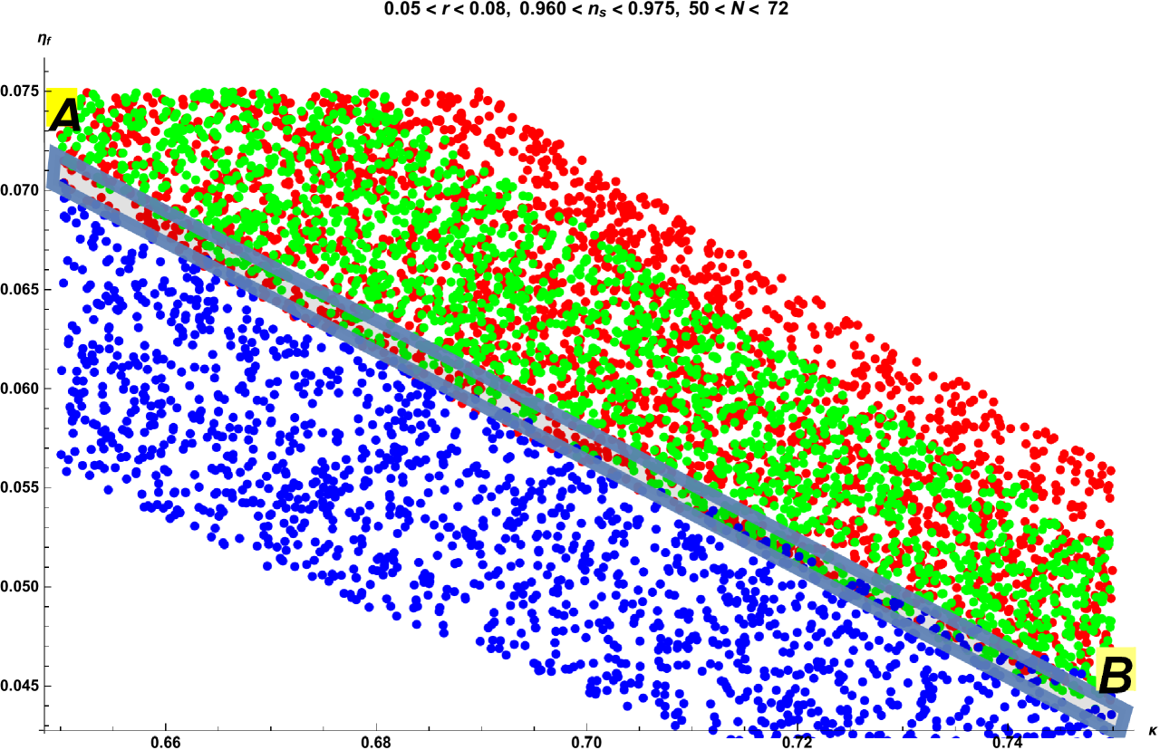
Figure 1: This plot depicts ranges of $\kappa$ and $\eta_{f}$ .

$\eta_{f}$	$\kappa$	$n_{s}$	$r$	$\mathrm{N}$
0.04611	0.7401	0.9750	0.07652	71
0.04743	0.7358	0.9746	0.07761	70
0.04848	0.7320	0.9745	0.07815	70
0.04892	0.7296	0.9747	0.07778	70
0.05007	0.7257	0.9745	0.07850	70
0.05103	0.7220	0.9744	0.07875	70
0.05174	0.7194	0.9744	0.07900	70
0.05290	0.7149	0.9744	0.07920	70
0.05385	0.7116	0.9743	0.07961	70
0.05710	0.6996	0.9742	0.08026	70

Table 4: Data set for the inflationary parameters extracting $\eta_{f}$ and $\kappa$ from the common region as depicted in Fig-1.

Nonetheless, the present model behaves appreciably otherwise, as it exhibits post-Planckian energy scale of inflation, and also admits graceful exit. For example, taking into account $U(\phi)$ (55), we find the following expression from equation (50),

$$6{\alpha_{0}\over\phi}\mathrm{H}^{2}=m^{2}(\phi^{2}-{C_{0}\over m^{2}}).$$ (61)

Now, if we choose a mid range value of ${C_{0}\over m^{2}}=21.5M^{2}_{P}$, together with a mid range value of $\alpha_{0}=0.127M^{3}_{P}$, with,  $\phi_{i}=7.0M_{P}$, as depicted in the table 2 and table 3, we simply find,

$$\mathrm{H}^{2}=\frac{m^{2}(\phi^{3}-{C_{0}\phi\over m^{2}})}{6\alpha_{0}},\hskip 21.68121pt\mathrm{and~{}hence},\hskip 21.68121pt\mathrm{H}^{2}\approx 253m^{2},$$ (62)

showing consistency with our data set displayed in Table 2 and Table 3. So, the energy scale of inflation$(\mathrm{H_{*}}\approx 15.9m)$ is sub-Planckian, since as mentioned earlier,$m\approx 10^{-5}M_{P}$. Further, since $r\approx 0.09$ for the above choice of $\alpha_{0}$, so we can easily calculate the energy scale of inflation $\mathrm{H_{*}}$ using the formula for single scalar field model as [72],

$$\mathrm{H_{*}}=8\times 10^{13}{\sqrt{r\over 0.2}}GeV=5.36\times 10^{13}GeV\approx 2.2\times 10^{-5}M_{P}.$$ (63)

$\mathrm{H}_{*}$ in the present case is just one order of magnitude higher than the single field inflation, which is the outcome of the redefined potential containing all the information regarding higher order terms and interactions.

As mentioned the model gracefully exits from inflation as well, since as $\phi\ll 1M_{P}$, it executes oscillatory behaviour, as shown below. Let us now express equation (50) as,

$$3\mathrm{H}^{2}={1\over 2\alpha}\left({1\over 2}\dot{\phi}^{2}+m^{2}\phi^{2}-C_{0}\right),$$ (64)

taking, $U(\phi)=m^{2}\phi^{2}-C_{0}$. In view of the expression of $\alpha(\phi)={\alpha_{0}\over\phi}$, the above equation reads as,

$${3\mathrm{H}^{2}\over m^{2}}={\phi\over 2\alpha_{0}}\left({\dot{\phi}^{2}\over 2m^{2}}+\phi^{2}-{C_{0}\over m^{2}}\right).$$ (65)

Note that, for GTR associated with non-minimally coupled single scalar field model, the above equation simplifies to: $3\mathrm{H}^{2}={1\over 2M_{p}^{2}}(\dot{\phi}^{2}+2m^{2}\phi^{2}-2C_{0})$. Since as inflation ends, ${\phi\over 2\alpha_{0}}\sim{28M_{p}^{-2}}$ according to the present data set, so as the Hubble rate ($\mathrm{H}$) falls below $m$, this equation (65) can be approximated to,

$$\dot{\phi}^{2}\approx-2(m^{2}\phi^{2}-C_{0}),$$ (66)

which may be integrated to yield,

$$\phi(t)=\pm\frac{\sqrt{C_{0}}\tan\left[m(\sqrt{2}t-t_{0})\right]}{m\sqrt{\tan^{2}\left[m(\sqrt{2}t-t_{0})\right]+1}},$$ (67)

and may further be simplified to obtain

$$\phi(t)=\pm\frac{\sqrt{C_{0}}}{m}\sin\left[m(\sqrt{2}t-t_{0})\right].$$ (68)

Where $t_{0}$ is the constant of integration. Thus the scalar field starts oscillating many times over a Hubble time, driving a matter-dominated era when inflation terminates.

4.3 Case-3:

Since, other than the value of $r$, the model behaves appreciably, it needs further study. In this subsection, we consider the last and the most legitimate (the reason will be clear shortly) choice of the effective potential as,

$$U=V+2\alpha\Lambda+6\alpha{\dot{\mathrm{H}}}-24\beta\mathrm{H}^{4}.$$ (69)

A comparison with (47) reveals that, the present potential (69) is cast excluding the term $-12\alpha\mathrm{H}^{2}$ and including $6\alpha\dot{\mathrm{H}}$,instead. This choice (69) again leads to klein-Gordon equation (26). Further, if we choose

$$U=V+2\alpha\Lambda-24\beta^{\prime}{\dot{\phi}}\mathrm{H}^{3}+576\gamma_{0}\mathrm{H}^{8},$$ (70)

excluding$-6\alpha^{\prime}{\dot{\phi}}\mathrm{H}$ term from (49), Friedman equation (25) may also be retrieved. Now, from (69), one can express $U=U(\phi)$ as,

$$U=\lambda^{2}\phi^{2}-576\gamma_{0}{\lambda}^{8}+\frac{12\alpha_{0}{\lambda}^{2}}{\phi}=m^{2}\phi^{2}+\frac{12\alpha_{0}m^{2}}{\phi}-C_{0},$$ (71)

where the solutions of $V,~{}\beta$ are substituted from equation (12), with the choice ${\lambda}^{2}=m^{2},~{}576\gamma_{0}{\lambda}^{8}=C_{0}$ and neglecting the term $6\alpha{\dot{\mathrm{H}}}$, since ${\dot{\mathrm{H}}}$ is nearly constant during inflation. The reason for considering the effective potentials in the above forms (69), and (70), is unveiled from the following scalar-tensor theoretic action of gravity,

$$A=\int\left[\alpha(\phi)R-{1\over 2}\phi_{,\mu}\phi^{,\mu}-U(\phi)\right]\sqrt{-g}~{}d^{4}x.$$ (72)

The above action (72) leads to the following field equations in the R-W space-time (3) under present consideration,

$$6\alpha{\dot{a}^{2}\over a^{2}}=-6\alpha^{\prime}{\dot{a}\over a}\dot{\phi}+U+{1\over 2}{\dot{\phi}}^{2};\hskip 28.45274pt{\ddot{\phi}}+3{\dot{a}\over a}\dot{\phi}=-U^{\prime}+6\alpha^{\prime}{\left({\ddot{a}\over a}-{\dot{a}^{2}\over a^{2}}\right)}+12\alpha^{\prime}{\dot{a}^{2}\over a^{2}}.$$ (73)

The field equations (25) and (26) are retrieved from the above pair under substitution of the expression of $U$ chosen in (70) and (69) respectively. The theory has thus been reduced to a scalar-tensor theory of gravity. Now, there are two independent ways to study inflation. The first is to proceed as before in the Jordan frame, and the second is to translate the action in Einstein frame and proceed. We study these two cases in the following two subsections.

4.3.1 Inflation in Jordan frame:

In view of the expression for $U(\phi)$ (71) the following inflationary parameters are found:

$$\begin{split}\epsilon&={\alpha_{0}\over\phi}\left(\frac{2\phi-{12\alpha_{0}\over\phi^{2}}}{\phi^{2}+{12\alpha_{0}\over\phi}-{C_{0}\over m^{2}}}\right)^{2}+{\alpha_{0}\over\phi^{2}}\left(\frac{2\phi-{12\alpha_{0}\over\phi^{2}}}{\phi^{2}+{12\alpha_{0}\over\phi}-{C_{0}\over m^{2}}}\right);\\ &\eta={2\alpha_{0}\over\phi}\left(\frac{2+{24\alpha_{0}\over\phi^{3}}}{\phi^{2}+{12\alpha_{0}\over\phi}-{C_{0}\over m^{2}}}\right);\hskip 56.9055pt\mathrm{N}={1\over 2\alpha_{0}}\int_{\phi_{f}}^{\phi_{i}}{\phi(\phi^{2}+{12\alpha_{0}\over\phi}-{C_{0}\over m^{2}})\over{(2\phi-{12\alpha_{0}\over\phi^{2}})}}d\phi.\end{split}$$ (74)

${C_{0}\over m^{2}}$ in $M^{2}_{P}$	$\phi_{f}$ in $M_{P}$	$n_{s}$	$r$	$\mathrm{N}$
144.18	0.84318	0.96502	0.01995	47
144.20	0.84314	0.96504	0.01991	51
144.22	0.84310	0.96506	0.01988	54
144.24	0.84306	0.96508	0.01985	57
144.26	0.84302	0.96510	0.01981	59
144.28	0.84298	0.96511	0.01978	62

Table 5: Data set for the inflationary parameters taking $\phi_{i}=7.26M_{P}$; $\alpha_{0}=2.0{M^{3}_{P}}$

$\alpha_{0}$ in $M^{3}_{P}$	$\phi_{f}$ in $M_{P}$	$n_{s}$	$r$	$\mathrm{N}$
0.0074	6.96004	0.9707	0.08113	53
0.0075	6.96025	0.9703	0.08222	53
0.0076	6.96045	0.9699	0.08331	52
0.0077	6.96066	0.9696	0.08440	51
0.0078	6.96086	0.9691	0.08550	51
0.0079	6.96107	0.9688	0.08659	50
0.0080	6.96127	0.9684	0.08768	49

Table 6: Data set for the inflationary parameters taking $\phi_{i}=7.40M_{P}$; ${C_{0}\over m^{2}}=48{M^{2}_{P}}$

A pair of data sets are exhibited in Table-5 and Table-6. Table-5, in which ${C_{0}\over m^{2}}$ is varied in the range $144.18M_{P}^{2}<{C_{0}\over m^{2}}<144.28M_{P}^{2}$, keeping $\phi_{i}=7.26M_{P}$ and $\alpha_{0}=2.0M_{P}^{3}$, shows tremendous fit with observation. On the contrary, Table-6, in which ${\alpha_{0}}$ is varied in the range $.0074M_{P}^{3}<{\alpha_{0}}<.0080M_{P}^{3}$, keeping $\phi_{i}=7.40M_{P}$, and ${C_{0}\over m^{2}}=48M_{P}^{2}$, shows nothing better than previous results obtained in earlier cases (Table-1 to Table-4). Note that in Table-6, $n_{s}$ is kept within the observational limit.

Since in earlier cases we have shown that the results are independent of the choice of the parameters of the theory the excellent fit in Table-5 therefore develops curiosity, and requires further study. Let us therefore proceed to find the energy scale of inflation. Using the above form of $U(\phi)$ (71), we procure the following expression from equation (50),

$$6{\alpha_{0}\over\phi}\mathrm{H}^{2}=m^{2}\phi^{2}+{12\alpha_{0}m^{2}\over\phi}-C_{0},~{}~{}\mathrm{or,}~{}~{}\mathrm{H}^{2}=\frac{6\alpha_{0}}{m^{2}}\left(\phi^{3}+12\alpha_{0}-{C_{0}\phi\over m^{2}}\right).$$ (75)

Taking $\phi_{i}=7.26M_{P},~{}{C_{0}\over m^{2}}=144.22M_{P}^{2},~{}\alpha_{0}=2M_{P}^{3},$ from table-5 we find,

$$\mathrm{H}^{2}=-53.37m^{2}M_{P}^{2},$$ (76)

Unfortunately, the wonderful fit of the present theory with observational data appears at a high price, viz. imaginary value of the energy scale, and therefore the data of Table-5 should be disregarded. On the contrary, the data presented in Table-6, viz. $\phi_{i}=7.40M_{P},~{}{C_{0}\over m^{2}}=48M_{P}^{2},~{}\alpha_{0}=.008M_{P}^{3}$ yields $\mathrm{H}^{2}=522m^{2}M_{P}^{2}$, and so the energy scale of inflation is $\mathrm{H_{*}}=2.3\times 10^{-4}M_{P}$, taking $m^{2}\approx 10^{-10}M_{P}^{2}$, which is again sub-Planckian.

4.3.2 Inflation in Einstein frame:

So far our study in all the above cases reveals that in no way, the tensor to scalar ratio may be reduced and matched with recent observation, keeping the scalar tilt within the observational limit ($0.9631\leq n_{s}\leq 0.9705$), and the number of e-folds within reasonable range $45<\mathrm{N}<70$. Finally, in the current subsection we study inflation in Einstein’s frame to explore better result in any. The Jordan frame action (LABEL:A3) can be translated to the Einstein-frame under the conformal transformation, $g_{E\mu\nu}=f(\phi)g_{\mu\nu}$ [73],[74] as,

$$A_{E}=\int\left[R_{E}-{1\over 2}\sigma_{E,\mu}\sigma^{E,\mu}-U_{E}(\sigma)\right]\sqrt{-g_{E}}~{}d^{4}x,$$ (77)

where, the subscript $`E$’ denotes Einstein’s frame. The above action (LABEL:A3) leads to the following field equations,

$$3\mathrm{H}^{2}=U_{E}+{1\over 2}{\dot{\sigma}}^{2};\hskip 28.45274pt\mathrm{and}\hskip 28.45274pt{\ddot{\sigma}}+3\mathrm{H}{\dot{\sigma}}=-U^{\prime}_{E},$$ (78)

where $U_{E}={U(\phi)\over{\alpha(\phi)}^{2}}$ and $(\sigma^{\prime})^{2}=\left(\frac{d\sigma}{d\phi}\right)^{2}=\frac{1}{\alpha(\phi)}+3\frac{\alpha^{\prime}(\phi)^{2}}{\alpha(\phi)^{2}}$. In the present case $\alpha(\phi)={\alpha_{0}\over\phi}$ and $(\sigma^{\prime})^{2}=\frac{\phi}{\alpha_{0}}+\frac{3}{\phi^{2}}$, and $U(\phi)=m^{2}\phi^{2}+\frac{12m^{2}\alpha_{0}}{\phi}-C_{0}$. The slow roll parameters can be written as shown in [74], in the following forms,

$$\epsilon=\left(\frac{U^{\prime}_{E}}{U_{E}}\right)^{2}\left(\frac{d\sigma}{d\phi}\right)^{-2}=\left[\frac{4\phi^{3}+12\alpha_{0}-2{C_{0}\phi\over m^{2}}}{\phi^{4}+12\alpha_{0}\phi-{C_{0}\phi^{2}\over m^{2}}}\right]^{2}{1\over({\phi\over\alpha_{0}}+{3\over\phi^{2}})},$$ (79)

$$\begin{split}\eta&=2\left[{\frac{U^{\prime\prime}_{E}}{U_{E}}}\left(\frac{d\sigma}{d\phi}\right)^{-2}-{\frac{U^{\prime}_{E}}{U_{E}}}\left(\frac{d\sigma}{d\phi}\right)^{-3}\frac{d^{2}\sigma}{d\phi^{2}}\right]\\ &=2\left[\frac{12\phi^{2}-2{C_{0}\over m^{2}}}{\left(\phi^{2}+\frac{12\alpha_{0}}{\phi}-{C_{0}\over m^{2}}\right)({\phi^{3}\over\alpha_{0}}+3)}-\frac{\left(4\phi^{3}+12\alpha_{0}-2{C_{0}\over m^{2}}\phi\right)\left({1\over\alpha_{0}}-{6\over\phi^{3}}\right)}{2\phi^{2}\left(\phi^{2}+\frac{12\alpha_{0}}{\phi}-{C_{0}\over m^{2}}\right)({\phi\over\alpha_{0}}+{3\over\phi^{2}})^{2}}\right].\end{split}$$ (80)

$$\mathrm{N}={1\over 2}\int{d\phi\over\epsilon(\phi)}{d\sigma\over d\phi}={1\over 2}\int\left({\phi\over\alpha_{0}}+{3\over\phi^{2}}\right)\left(\frac{\phi^{4}+12\alpha_{0}\phi-{C_{0}\phi^{2}\over m^{2}}}{4\phi^{3}+12\alpha_{0}-2{C_{0}\phi\over m^{2}}}\right){d\phi}.$$ (81)

${\alpha_{0}}$ in $M^{2}_{P}$	$\phi_{f}$ in $M_{P}$	$n_{s}$	$r$	$\mathrm{N}$
0.0061	7.0999	0.9701	0.09226	51
0.0062	7.1002	0.9697	0.09377	50
0.0063	7.1004	0.9692	0.09528	49
0.0064	7.1006	0.9687	0.09678	48
0.0065	7.1009	0.9682	0.09829	47
0.0066	7.1011	0.9676	0.09980	46

Table 7: Data set for the inflationary parameters taking $\phi_{i}=7.5M_{P}$; ${C_{0}\over m^{2}}=50{M^{2}_{P}}$

${C_{0}\over m^{2}}$ in $M^{2}_{P}$	$\phi_{f}$ in $M_{P}$	$n_{s}$	$r$	$\mathrm{N}$
140	0.92287	0.96114	0.02563	65
142	0.92213	0.96145	0.02698	64
144	0.92141	0.96173	0.02825	64
146	0.92071	0.96199	0.02952	63
148	0.92003	0.96224	0.03077	62
150	0.91937	0.96246	0.03199	62

Table 8: Data set for the inflationary parameters taking $\phi_{i}=7.0M_{P}$; $\alpha_{0}=0.65{M^{3}_{P}}$

Here we present two tables, viz. Table-7 and Table-8. It appears that Table-8 fits observational data with extreme precession. Let us, therefore explore the energy scale of inflation for both the cases. Considering the above form of $U_{E}(\phi)$ (69), we obtain the following expression from equation (50),

$$3\mathrm{H}^{2}=(m^{2}\phi^{2}+\frac{12m^{2}\alpha_{0}}{\phi}-C_{0})=m^{2}(\phi^{2}+\frac{12\alpha_{0}}{\phi}-{C_{0}\over m^{2}}).$$ (82)

Now, taking $\phi_{i}=7.5M_{P},~{}{C_{0}\over m^{2}}=50M_{P}^{2},~{}\alpha_{0}=0.0064M_{P}^{3},$ from Table-7 one can get,

$$3\mathrm{H}^{2}={(56.25+0.01024-50)m^{2}},~{}~{}~{}or,~{}~{}\mathrm{H}^{2}=2.08\times 10^{-10}M_{P}^{2},$$ (83)

with $m^{2}\approx 10^{-10}M_{P}^{2}$. So, the energy scale of inflation is $(\mathrm{H_{*}}\approx 1.44\times 10^{-5}M_{P})$ is sub-Planckian and fits with single field energy scale perfectly. On the contrary, taking $\phi_{i}=7.0M_{p},~{}{C_{0}\over m^{2}}=146M_{P}^{2},~{}\alpha_{0}=0.65M_{P}^{3},$ from Table-8 one obtains,

$$\mathrm{H}^{2}=\frac{(49+1.11-146)m^{2}}{3},~{}~{}~{}\mathrm{H_{*}}^{2}=-32\times 10^{-10}M^{2}_{P},$$ (84)

with $m^{2}\approx 10^{-10}M_{P}^{2}$. So, the energy scale of inflation is negative, and hence data in Table-8 are faulty. In a nut-shell, present analysis exhibits that the inflationary parameters remain unaffected under different choices of the redefined potentials, together with the one in Einstein’s frame. It has also been shown that the inflationary parameters are independent of the choice of the parameters of the theory.

5 Cosmic evolution in the matter dominated era:

At this end we observe that, the gravitational action for non-minimally coupled scalar-tensor theory, being supplemented by a Gauss-Bonnet term with scalar coupling and a Gauss-Bonnet squared term, leads to a well-behaved quantum picture (The effective Hamiltonian is hermitian, standard quantum mechanical probabilistic interpretation holds, and transition over to the classical universe under a viable semi-classical approximation is admissible). However, the action is not quite consistent with recent observational constraints on inflationary parameters. It’s true that the action is well suited to act as an alternative to dark energy at the very late stage of cosmic evolution. It is therefore necessary to study cosmic evolution in the middle - the radiation dominated era which initiated soon after graceful exit from inflation, and the early pressure-less dust era. The oscillation of the scalar field produces particles which heats up the universe whence it enters the so called ‘hot big bang’ era, which is the onset of radiation dominated era. All the essential features at this era (structure formation and the formation of CMBR right in time) are perfectly described by the Friedmann-solution ($a=a_{0}\sqrt{t}$). With the evolution, the universe reaches a stage called ‘matter-radiation equality’ at a redshift around $z\sim 3200$. Thereafter matter takes over radiation and the universe enters a pressureless dust era. This era again is best described by Friedmann solution ($a\propto t^{2\over 3}$) until recently ($z\sim 1$), whence the universe evolves with accelerated expansion. Note that, the de-Sitter solution has already fixed the forms of the coupling parameters $\alpha(\phi)={\alpha_{0}\over\phi},~{}\beta(\phi)=-{\alpha_{0}\beta_{0}\over\phi}-\beta_{1}\phi^{2}$, and $\gamma(\phi)=\gamma_{0}$ = constant, along with the potential $V(\phi)=m^{2}\phi^{2}-V_{0}$ (12), and in no way one can consider else.

To study the evolutions in the matter-dominated (radiation and early pressureless dust) eras, we therefore write the field equations (6), (7) and (8) in flat space $k=0$, including a barotropic fluid, and substituting the forms of $\alpha(\phi),~{}\beta(\phi),~{}\gamma(\phi)=\gamma_{0}$ etc., along with potential $V(\phi)$ obtained for de-Sitter solution in (12) as,

$$\begin{split}&2{\alpha_{0}\over\phi}\left({\ddot{z}\over z}-{\dot{z}^{2}\over 4z^{2}}-\Lambda\right)-2{\alpha_{0}\over\phi^{2}}\left({\ddot{\phi}}+{\dot{\phi}}{\dot{z}\over z}\right)+4{\alpha_{0}\over\phi^{3}}{\dot{\phi}^{2}}-\frac{{\dot{\phi}^{2}}\dot{z}^{2}}{z^{2}}\left[{1\over 12\lambda^{2}}+{2\alpha_{0}\over\phi^{3}}\left(\frac{1}{\lambda^{2}}-\frac{\Lambda}{6\lambda^{4}}\right)\right]\\ &\hskip 21.68121pt+\left\{\frac{2{\dot{\phi}}\dot{z}\ddot{z}}{z^{2}}\left[-{\phi\over 12\lambda^{2}}+{\alpha_{0}\over\phi^{2}}\left(\frac{1}{\lambda^{2}}-\frac{\Lambda}{6\lambda^{4}}\right)\right]+\frac{{\ddot{\phi}}\dot{z}^{2}}{z^{2}}\left[-{\phi\over 12\lambda^{2}}+{\alpha_{0}\over\phi^{2}}\left(\frac{1}{\lambda^{2}}-\frac{\Lambda}{6\lambda^{4}}\right)\right]\right\}\\ &\hskip 21.68121pt+12\gamma_{0}\left[{\dot{z}^{4}{\ddddot{z}}\over z^{5}}+{8\dot{z}^{3}\ddot{z}\dddot{z}\over z^{5}}-{9\dot{z}^{5}\dddot{z}\over z^{6}}+{6\dot{z}^{2}\ddot{z}^{3}\over z^{5}}-{135\dot{z}^{4}\ddot{z}^{2}\over 4z^{6}}+{159\dot{z}^{6}\ddot{z}\over 4z^{7}}-{195\dot{z}^{8}\over 16z^{8}}\right]\\ &\hskip 21.68121pt-\frac{{\dot{\phi}}\dot{z}^{3}}{z^{3}}\left[-{\phi\over 12\lambda^{2}}+{\alpha_{0}\over\phi^{2}}\left(\frac{1}{\lambda^{2}}-\frac{\Lambda}{6\lambda^{4}}\right)\right]=-\omega{\rho_{0}}{a^{-3(1+\omega)}}-\Big{[}{1\over 2}\dot{\phi}^{2}-\left({\lambda^{2}\phi^{2}\over 2}-C_{0}\right)\Big{]};\\ &2{\alpha_{0}\over\phi}\left({3\dot{z}^{2}\over 4z^{2}}-\Lambda\right)-{3\alpha_{0}\dot{\phi}\dot{z}\over\phi z}+{3\dot{\phi}\dot{z}^{3}\over z^{3}}\left[-{\phi\over 24\lambda^{2}}+{\alpha_{0}\over\phi^{2}}\left(\frac{1}{2\lambda^{2}}-\frac{\Lambda}{12\lambda^{4}}\right)\right]\\ &\hskip 21.68121pt+18\gamma_{0}\left[{\dot{z}^{5}\dddot{z}\over z^{6}}+{3\dot{z}^{4}\ddot{z}^{2}\over 2z^{6}}-{9\dot{z}^{6}\ddot{z}\over 2z^{7}}+{15\dot{z}^{8}\over 8z^{8}}\right]={\rho_{0}}{a^{-3(1+\omega)}}+{1\over 2}\dot{\phi}^{2}+{\lambda^{2}\phi^{2}\over 2}-C_{0};\\ &\ddot{\phi}+{3\over 2}{\dot{z}\over z}\dot{\phi}+{3\alpha_{0}\ddot{z}\over z\phi^{2}}-2\Lambda{\alpha_{0}\over\phi^{2}}-{3\dot{z}^{2}\ddot{z}\over z^{3}}\left[-{\phi\over 24\lambda^{2}}+{\alpha_{0}\over\phi^{2}}\left(\frac{1}{2\lambda^{2}}-\frac{\Lambda}{12\lambda^{4}}\right)\right]\\ &\hskip 21.68121pt+{{3\dot{z}^{4}}\over 2z^{4}}\left[-{\phi\over 24\lambda^{2}}+{\alpha_{0}\over\phi^{2}}\left(\frac{1}{2\lambda^{2}}-\frac{\Lambda}{12\lambda^{4}}\right)\right]+\lambda^{2}\phi=0.\end{split}$$ (85)

Let us now seek a power law solution $a\propto t^{n}$ i.e. $z=a^{2}=c^{2}(t)^{2n}$ (say) and $\phi=\phi_{0}t^{-m}$(say), using the barotropic equation of state, $p={\omega\rho}$, where, $\omega={1\over 3}$ for radiation dominated era and $\omega=0$ for pressureless dust era. The Bianchi identity $\dot{\rho}+3{\dot{a}\over a}(\rho+\omega\rho)=0$ therefore results in,

$$\rho=\rho_{0}a^{-3(1+\omega)},$$ (86)

where, $\rho_{0}$ represents the value of the density (radiation or matter) available in the present universe. The above set of field equations (LABEL:fe1) are therefore expressed as:

$$\begin{split}&{2\alpha_{0}\over\phi_{0}t^{-m}}\left({2n(2n-1)\over t^{2}}-{n^{2}\over t^{2}}-\Lambda\right)-{2\alpha_{0}\over\phi_{0}^{2}t^{-2m}}\left({\phi_{0}m(m+1)\over t^{(}m+2)}-{2nm\phi_{0}\over t^{m+2}}\right)\\ &\hskip 21.68121pt+\frac{4\alpha_{0}m^{2}}{\phi_{0}t^{-m+2}}-\frac{4n^{2}m^{2}\phi_{0}^{2}}{t^{2(m+2)}}\left[{1\over 12\lambda^{2}}+{2\alpha_{0}\over\phi_{0}^{3}t^{-3m}}\left(\frac{1}{\lambda^{2}}-\frac{\Lambda}{6\lambda^{4}}\right)\right]\\ &\hskip 21.68121pt+\frac{4n^{2}m(m+3-2n)\phi_{0}}{t^{(m+4)}}\left[-{\phi_{0}t^{-m}\over 12\lambda^{2}}+{\alpha_{0}\over\phi_{0}^{2}t^{-2m}}\left(\frac{1}{\lambda^{2}}-\frac{\Lambda}{6\lambda^{4}}\right)\right]\\ &\hskip 21.68121pt+12\gamma_{0}\left[\frac{32n^{5}(2n-1)(2n-2)(2n-3)}{t^{8}}+\frac{256n^{5}(2n-1)^{2}(2n-2)}{t^{8}}-\frac{576n^{6}(2n-1)(2n-2)}{t^{8}}\right]\\ &\hskip 21.68121pt+12\gamma_{0}\left[\frac{192n^{5}(2n-1)^{3}}{t^{8}}-\frac{2160n^{6}(2n-1)^{2}}{t^{8}}+\frac{5088n^{7}(2n-1)}{t^{8}}-\frac{3120n^{8}}{t^{8}}\right]\\ &\hskip 21.68121pt=-{\omega\rho_{0}\over c^{3(1+\omega)}t^{3n(1+\omega)}}-{m^{2}\phi_{0}^{2}\over 2t^{2(m+1)}}+{{\lambda^{2}\phi_{0}^{2}t^{-2m}}\over 2}-C_{0}.\end{split}$$ (87)

$$\begin{split}&{2\alpha_{0}\over\phi_{0}t^{-m}}\left({3n^{2}\over t^{2}}-\Lambda\right)+\frac{6\alpha_{0}nm}{t^{2}}-\frac{24m\mathrm{}n^{3}\phi_{0}}{t^{m+4}}\left[-{\phi_{0}t^{-m}\over 24\lambda^{2}}+{\alpha_{0}\over\phi_{0}^{2}t^{-2m}}\left(\frac{1}{2\lambda^{2}}-\frac{\Lambda}{12\lambda^{4}}\right)\right]\\ &\hskip 21.68121pt+18\gamma_{0}\left[\frac{64n^{6}(2n-1)(2n-2)}{t^{8}}+\frac{96n^{6}(2n-1)^{2}}{t^{8}}-\frac{576n^{7}(2n-1)}{t^{8}}+\frac{480n^{8}}{t^{8}}\right]\\ &\hskip 21.68121pt={\rho_{0}\over c^{3(1+\omega)}t^{3n(1+\omega)}}+{m^{2}\phi_{0}^{2}\over 2t^{2(m+1)}}+{{\lambda^{2}\phi_{0}^{2}t^{-2m}}\over 2}-C_{0}.\end{split}$$ (88)

$$\begin{split}&{m(m+1)\phi_{0}\over t^{m+2}}-{3nm\phi_{0}\over t^{m+2}}+\frac{6\alpha_{0}n(2n-1)}{\phi_{0}^{2}t^{2-2m}}-{{2\alpha_{0}\Lambda}\over\phi_{0}^{2}t^{-2m}}-\frac{24n^{3}(2n-1)}{t^{4}}\left[-{\phi_{0}t^{-m}\over 24\lambda^{2}}+{\alpha_{0}\over\phi_{0}^{2}t^{-2m}}\left(\frac{1}{2\lambda^{2}}-\frac{\Lambda}{12\lambda^{4}}\right)\right]\\ &\hskip 21.68121pt+\frac{24n^{4}}{t^{4}}\left[-{\phi_{0}t^{-m}\over 24\lambda^{2}}+{\alpha_{0}\over\phi_{0}^{2}t^{-2m}}\left(\frac{1}{2\lambda^{2}}-\frac{\Lambda}{12\lambda^{4}}\right)\right]+\lambda^{2}\phi_{0}t^{-m}=0.\end{split}$$ (89)

Now, equation (89) may only be satisfied for $n={1\over 2}$, provided $m=0$, $\alpha_{0}={\phi_{0}^{3}\over 6}$ and $\Lambda=3\lambda^{2}$. Note that, $m=0$ simply implies $\phi=\phi_{0}~{}\text{(constant)}$. This means a viable matter dominates era may be realized if the scalar field seizes to evolve any further. This as such does not create any problem, since it has been revealed that a possible transition from decelerated to accelerated pressureless dust dominated epoch, admitting phantom phases, naturally appear in the framework of $F(R,\mathcal{G})$, without opting for a scalar field [26, 27].

5.1 Radiation dominated era:

In the radiation dominated era, $\omega={1\over 3}$, and hence $\rho={\rho_{r0}\over a^{4}}$, in view of equation (86), where, $\rho_{r0}$ is the amount of radiation density available in the present universe. As mentioned, equation (89) is satisfied only for $n={1\over 2}$ and $m=0$, in which case, the first two equations (87) and(88) reduce to,

$$\begin{split}&{\alpha_{0}\over 2\phi_{0}t^{2}}+{2\alpha_{0}\Lambda\over\phi_{0}}+{585\gamma_{0}\over 4t^{8}}={\rho_{r0}\over 3c^{2}t^{2}}-{\lambda^{2}\phi_{0}^{2}\over 2}+C_{0},\end{split}$$ (90)

and

$$\begin{split}&{3\alpha_{0}\over 2\phi_{0}t^{2}}-{2\alpha_{0}\Lambda\over\phi_{0}}+{135\gamma_{0}\over 4t^{8}}={\rho_{r0}\over c^{2}t^{2}}+{\lambda^{2}\phi_{0}^{2}\over 2}-C_{0}.\end{split}$$ (91)

The above two equations are satisfied once we can neglect $t^{-8}$ term associated with $(\mathcal{G})^{2}$. However, since the universe enters hot big bang era at around ($t\sim 10^{-18\pm 6}$s), so in the early radiation era $t^{-8}$ term gives dominant contribution. Hence, the cosmic evolution of early radiation era will typically be different from the standard model, which might tell upon structure formation. Nonetheless, at the late stage, this term may be safely neglected. In that case, we are simply left with Friedmann equation along with an effective cosmological constant, and the above pair of equations are satisfied for $C_{0}={\lambda^{2}\phi_{0}^{2}\over 2}+{2\alpha_{0}\Lambda\over\phi_{0}}={3\lambda^{2}\phi_{0}^{2}\over 2}$, and $\rho_{r0}=\frac{3\alpha_{0}c^{2}}{2\phi_{0}}={\phi_{0}^{2}c^{2}\over 4}$. Note that, one can add a term $b_{0}\mathcal{G}^{n_{2}}$ at this stage with $n_{2}<{1\over 2}$. Unfortunately, the field equations in no way are satisfied, unless $b_{0}=0$. We remind, it was demonstrated that the form $F(\mathcal{G})=a_{0}\mathcal{G}^{n_{1}}+b_{0}\mathcal{G}^{n_{2}}$ can unify early inflationary era (if $n_{1}>1$) with late-time accelerated expansion, (if $n_{2}<{1\over 2}$) [27]. Since a viable radiation era does not admit $n_{2}<{1\over 2}$, late-time acceleration in the pressureless dust era with powers of Gauss-Bonnet term is questionable. Further, since we have already shown that no other than $a\propto\sqrt{t}$ satisfies the field equations, a viable ($a\propto t^{2\over 3}$, as in the standard model of cosmology) early pressureless dust era also remains obscure.

6 Concluding remarks:

It was argued that $F(\mathcal{G})=a_{0}\mathcal{G}^{n_{1}}+b_{0}\mathcal{G}^{n_{2}}$ can unify early inflationary phase (if $n_{1}>1$) and late-time accelerating phase, (if $n_{2}<{1\over 2}$). However, in no way one can disregard a dilatonic coupled Gauss-Bonnet term in the very early epoch, since it is an artefact of different string inspired theories. Taking into account a scalar-tensor theory of gravity, associated with dilatonic coupled Gauss-Bonnet term and a Gauss-Bonnet squared term, we study inflation. Inflation was triggered at a very early epoch, when all the fields but gravity are quantized. Therefore, prior to study inflationary dynamics from classical field equation, it is suggestive to construct the quantum counterpart of the theory and to see if a legitimate semiclassical wave function emerges. This we have performed and studied inflation thereafter.

For a theory having additional degrees of freedom in the form of coupling parameters, classical field equations are usually reduced to Friedmann-like equations under the choice of additional hierarchy of flow parameters. Earlier, for a single additional degree of freedom, the technique worked nicely. However, in the present situation we had a couple of independent coupling parameters requiring two additional choices. This reduced the field equations substantially, without reflecting the contribution from Gauss-Bonnet-dilatonic term and the Gauss-Bonnet squared term. We have therefore followed a different method to reduce the extremely complicated set of field equations considerably, by choosing effective potentials. We have studied three independent cases for three different choices of the redefined potentials, and find that the inflationary parameters remain almost unaltered. The last case have been studied both in Jordan as well as Einstein’s frames and no remarkable change in the inflationary parameters has been noticed. It has been shown that it is impossible to meet the present observational constraint on tensor to scalar ratio ($r<.032$), which might even be reduced in future experiments. It is noteworthy that our results are independent of the choice of the parameters of the theory.

Further, it is found that a viable radiation era is possible only at the late stage, prior to the pressureless dust era, provided the scalar field ceases to evolve and Gauss-Bonnet squared term is neglected. This might tell upon structure formation and also on the formation of CMBR at right epoch. The matter dominated era also evolves as $a\propto\sqrt{t}$, instead of $a\propto t^{2\over 3}$. Further, since a viable radiation era does not admit term like $\mathcal{G}^{n_{2}}$ for $n_{2}<{1\over 2}$, hence late stage accelerated expansion remains obscure. In a nut shell, present study reveals that the theory does not quite justify cosmological evolution in different regimes.

Data Availability Statement: The authors declare that all data supporting the findings of this study are available within the article.

CRediT authorship contribution statement: Dalia Saha: Computation, Cross-checking, Writing - review and editing. Jyoti Prasad Saha: Computation, Cross-checking, Writing - review and editing. Abhik Kumar Sanyal: Cross-checking, Supervision, Writing - original draft, Writing - review and editing.

Declaration of competing interest The authors declare that they have no known competing financial interests or personal relationships that could have appeared to influence the work reported in this paper.

Funding: We also declare that no funding is available for the present research from any organization.

Appendix A Appendix A: Phase space structure, Dirac’s algorithm:

In fact there are two known formalisms which can handle such singular action being associated with higher order terms, towards expressing it in canonical form. The first is the well known Dirac formalism. It works to produce a viable quantum theory, if applied after removing the total derivative terms present in the action, as we already have done, and expressed it in equation (2) and then finally in (LABEL:A3), under a change of variable. The other technique, known as ‘modified Horowitz’ formalism’ (MHF), bypasses Dirac’s constraint analysis, and works as well to produce identical phase-space structure. There is yet another formalism presented by Buchbinder and his collaborators, which we have recently explored (D.Saha and A.K. sanyal, Perusing Buchbinder-Lyakhovich Canonical Formalism for the Higher-Order Theory of Gravity, Universe, 9, 48, (2023)), and found viable to produce identical phase-space structure too. However, we are not considering it here. It is duly required to mention that all other techniques which do not take care of the divergent terms (inclusive of Dirac’s formalism), also produce phase-space structure of the Hamiltonian, which although different, are canonically equivalent. However, such equivalence remains obscure in the quantum domain, due to non-linearity, and the associated quantum counterparts run into problem [75]. Here, as mentioned we shall follow Dirac’s constraint analysis starting from the action (LABEL:A3), and in the Appendix B explore MHF, to prove equivalence between the two. The point Lagrangian in connection with the action (LABEL:A3) takes the following form,

$$\begin{split}L&=-{6\alpha(\phi)N}\Big{(}{x^{2}\over 4\sqrt{z}}-k\sqrt{z}+{\Lambda\over 3}z^{3\over 2}\Big{)}-{3\alpha^{\prime}(\phi)\dot{\phi}x\sqrt{z}}-\frac{\beta^{\prime}x\dot{\phi}}{\sqrt{z}}\bigg{(}\frac{x^{2}}{z}+12k\bigg{)}+Nz^{3\over 2}\Big{(}{1\over 2N^{2}}\dot{\phi}^{2}-V(\phi)\Big{)}\\ &+144\gamma(\phi)\Bigg{\{}{(x^{2}+4kz)^{2}\dot{x}^{2}\over 16Nz^{9\over 2}}+{\gamma^{\prime}(\phi)\dot{\phi}\over\gamma(\phi)}\Big{(}{x^{7}\over 112z^{11\over 2}}+{kx^{5}\over 10z^{9\over 2}}+{k^{2}x^{3}\over 3z^{7\over 2}}\Big{)}-N\Big{(}{15x^{8}\over 448z^{13\over 2}}+{13kx^{6}\over 40z^{11\over 2}}+{11k^{2}x^{4}\over 12z^{9\over 2}}\Big{)}\Bigg{\}}\\ &\hskip 28.90755pt+u\left({\dot{z}\over N}-x\right).\end{split}$$ (A.1)

Note that, as a result of the change of variable (16), expression $\big{(}{\dot{z}\over N}-x=0\big{)}$ turns out to be a constraint, which has been introduced in the above point Lagrangian through the Lagrange multiplier $u$. The canonical momenta therefore are,

$$\begin{split}&p_{\phi}=-{3\alpha^{\prime}x\sqrt{z}}+{z^{3\over 2}\dot{\phi}\over N}+144\gamma^{\prime}(\phi)\left({x^{7}\over 112z^{11\over 2}}+{kx^{5}\over 10z^{9\over 2}}+{k^{2}x^{3}\over 3z^{7\over 2}}\right)-\frac{\beta^{\prime}x}{\sqrt{z}}\bigg{(}\frac{x^{2}}{z}+12k\bigg{)},\\ &p_{x}=\left[{288\gamma\over N}\left({x^{4}\over 16z^{9\over 2}}+{kx^{2}\over 2z^{7\over 2}}+{k^{2}\over z^{5\over 2}}\right)\right]\dot{x},\hskip 28.90755ptp_{z}={u\over N},\hskip 28.90755ptp_{N}=0=p_{u},\end{split}$$ (A.2)

and the resulting constrained Hamiltonian reads as,

$$\begin{split}H_{c}=&{Np_{x}^{2}\over{576\gamma\left({x^{4}\over 16z^{9\over 2}}+{kx^{2}\over 2z^{7\over 2}}+{k^{2}\over z^{5\over 2}}\right)}}+\dot{z}{u\over N}+{Np_{\phi}^{2}\over 2z^{3\over 2}}\\ &+\left[{3N\alpha^{\prime}\over z}-{144N\gamma^{\prime}\over z^{3\over 2}}\left({x^{7}\over 112z^{11\over 2}}+{kx^{5}\over 10z^{9\over 2}}+{k^{2}x^{3}\over 3z^{7\over 2}}\right)\right]p_{\phi}+\bigg{(}\frac{x^{2}}{z}+12k\bigg{)}\left[\frac{N\beta^{\prime}xp_{\phi}}{z^{2}}+\frac{3N\alpha^{\prime}\beta^{\prime}x^{2}}{z^{3\over 2}}\right]\\ &-\left({x^{7}\over 112z^{11\over 2}}+{kx^{5}\over 10z^{9\over 2}}+{k^{2}x^{3}\over 3z^{7\over 2}}\right)\left[{432\alpha^{\prime}\gamma^{\prime}xN\over z}+{288N\beta^{\prime}\gamma^{\prime}x\over z}\bigg{(}\frac{x^{2}}{z}+12k\bigg{)}\right]\\ &+{9\alpha^{\prime 2}x^{2}N\over 2\sqrt{z}}+\frac{N\beta^{\prime 2}x^{2}}{2z^{5\over 2}}\bigg{(}\frac{x^{2}}{z}+12k\bigg{)}^{2}+{10368N\gamma^{\prime 2}\over z^{3\over 2}}\left({x^{7}\over 112z^{11\over 2}}+{kx^{5}\over 10z^{9\over 2}}+{k^{2}x^{3}\over 3z^{7\over 2}}\right)^{2}\\ &+{6\alpha N}\left({x^{2}\over 4\sqrt{z}}-k\sqrt{z}+{\Lambda\over 3}z^{3\over 2}\right)+36\gamma Nx^{4}\left({15x^{4}\over 112z^{13\over 2}}+{13kx^{2}\over 10z^{11\over 2}}+{11k^{2}\over 3z^{9\over 2}}\right)+NVz^{3\over 2}-\dot{z}{u\over N}+ux.\end{split}$$ (A.3)

The definitions of momenta (A.2) reveal that there exists following pair of primary constraints viz,

$$\phi_{1}=Np_{z}-u\approx 0,~{}\phi_{2}=p_{u}\approx 0,$$ (A.4)

which involve Lagrange multipliers or their conjugates. Note that the constraint $\phi_{3}=p_{N}$ associated with lapse function $N$ is non-dynamical, and so vanishes strongly. Thus it has been disregarded. The above two primary constraints (A.4) are second class, since their Poisson bracket with other constraints do not vanish. In two possible manner these second-class constraints may be tackled. Firstly, using arbitrary Lagrange multipliers, the constraints are inserted into the Hamiltonian, which may be determined explicitly. This helps to solve consistency equations, since $det|{\phi_{i},\phi_{j}}|\neq 0$. Second, introducing Dirac bracket, in which case the constraints are disregarded. Note that the correct commutation relations required to build the quantum theory follow from Dirac brackets, therefore let us compute Dirac brackets first, thereafter follow the first method, which is straight forward. In phase-space, the Dirac bracket of two functions $f_{1}$ and $f_{2}$ is defined as (we use $DB$, and $PB$ in the suffix to denote Dirac and Poisson brackets respectively).

$$\big{\{}f_{1},f_{2}\big{\}}_{DB}=\big{\{}f_{1},f_{2}\big{\}}_{PB}-\sum_{ij}\big{\{}f_{1},\phi_{i}\big{\}}_{PB}M^{-1}_{ij}\big{\{}\phi_{j},f_{2}\big{\}}_{PB},$$ (A.5)

where $M^{-1}_{ij}$ denotes the inverse of the matrix $M_{ij}=\big{\{}\phi_{i},\phi_{j}\big{\}}_{PB}$. In the present situation, the matrix and its inverse are simply

$$M_{ij}=\left(\begin{array}[]{cc}0&-1\\ 1&0\\ \end{array}\right)~{}~{}\mathrm{and}~{}~{}M^{-1}_{ij}=\left(\begin{array}[]{cc}0&1\\ -1&0\\ \end{array}\right)$$ (A.6)

and hence the Dirac bracket takes the following form:

$$\big{\{}f_{1},f_{2}\big{\}}_{DB}=\big{\{}f_{1},f_{2}\big{\}}_{PB}+\sum_{ij}\epsilon_{ij}\big{\{}f_{1},\phi_{i}\big{\}}_{PB}\big{\{}\phi_{j},f_{2}\big{\}}_{PB},$$ (A.7)

where $\epsilon_{ij}$ is the Levi-Civita symbol. One can now compute Dirac bracket in a straightforward manner to find,

$$\begin{split}\{z,p_{z}\}_{DB}&=\{z,p_{z}\}_{PB}+\epsilon_{11}\{z,\phi_{1}\}_{PB}\{\phi_{1},p_{z}\}_{PB}+\epsilon_{12}\{z,\phi_{1}\}_{PB}\{\phi_{2},p_{z}\}_{PB}\\ &\hskip 56.9055pt+\epsilon_{21}\{z,\phi_{2}\}_{PB}\{\phi_{1},p_{z}\}_{PB}+\epsilon_{22}\{z,\phi_{2}\}_{PB}\{\phi_{2},p_{z}\}_{PB}\\ &=\{z,p_{z}\}_{PB}=1,\end{split}$$ (A.8)

since, $\{\phi_{i},p_{z}\}_{PB}=0$. In the same way it is possible to show that: $\{x,p_{x}\}_{DB}=\{x,p_{x}\}_{PB}=1$, $\{z,p_{x}\}_{DB}=\{z,p_{x}\}_{PB}=0$,$\{p_{z},p_{x}\}_{DB}=\{p_{z},p_{x}\}_{PB}=0$. As a result, the standard commutation relations viz. $[\hat{z},\hat{p}_{z}]=i\hbar$, $[\hat{z},\hat{p}_{x}]=0$, hold for canonical quantization. The equality holds because $\phi_{2}$ vanishes strongly. So, in this prescription, it may be disregarded, as mentioned. However, this is not possible while following the first prescription, because in that case the Lagrange multipliers would remain undetermined. We now switch over to the standard procedure as already mentioned. So we substitute the two constraints, and as a result the modified primary Hamiltonian reads as,

$$H_{p1}=H_{c}+u_{1}(Np_{z}-u)+u_{2}p_{u}$$ (A.9)

In the above, we introduced the Lagrange multipliers $u_{1}$, $u_{2}$, and find that the Poisson brackets $\{x,p_{x}\}=\{z,p_{z}\}=\{u,p_{u}\}=\{\phi,p_{\phi}\}=1$, hold. The primary Hamiltonian therefore takes the following form,

$$\begin{split}H_{p1}=&N\Bigg{[}{p_{x}^{2}\over{576\gamma\left({x^{4}\over 16z^{9\over 2}}+{kx^{2}\over 2z^{7\over 2}}+{k^{2}\over z^{5\over 2}}\right)}}+{p_{\phi}^{2}\over 2z^{3\over 2}}+\left[{3\alpha^{\prime}x\over z}-{144\gamma^{\prime}\over z^{3\over 2}}\left({x^{7}\over 112z^{11\over 2}}+{kx^{5}\over 10z^{9\over 2}}+{k^{2}x^{3}\over 3z^{7\over 2}}\right)\right]p_{\phi}\\ &+\bigg{(}\frac{x^{2}}{z}+12k\bigg{)}\left[\frac{\beta^{\prime}xp_{\phi}}{z^{2}}+\frac{3\alpha^{\prime}\beta^{\prime}x^{2}}{z^{3\over 2}}\right]-\Big{(}{x^{7}\over 112z^{11\over 2}}+{kx^{5}\over 10z^{9\over 2}}+{k^{2}x^{3}\over 3z^{7\over 2}}\Big{)}\left[{432\alpha^{\prime}\gamma^{\prime}x\over z}+{288\beta^{\prime}\gamma^{\prime}x\over z}\bigg{(}\frac{x^{2}}{z}+12k\bigg{)}\right]\\ &+{9\alpha^{\prime 2}x^{2}N\over 2\sqrt{z}}+\frac{\beta^{\prime 2}x^{2}}{2z^{5\over 2}}\bigg{(}\frac{x^{2}}{z}+12k\bigg{)}^{2}+{10368\gamma^{\prime 2}\over z^{3\over 2}}\left({x^{7}\over 112z^{11\over 2}}+{kx^{5}\over 10z^{9\over 2}}+{k^{2}x^{3}\over 3z^{7\over 2}}\right)^{2}\\ &+{6\alpha}\left({x^{2}\over 4\sqrt{z}}-k\sqrt{z}+{\Lambda\over 3}z^{3\over 2}\right)+36\gamma x^{4}\left({15x^{4}\over 112z^{13\over 2}}+{13kx^{2}\over 10z^{11\over 2}}+{11k^{2}\over 3z^{9\over 2}}\right)+Vz^{3\over 2}\Bigg{]}\\ &+u_{1}\big{(}Np_{z}-u\big{)}+u_{2}p_{u}+ux.\end{split}$$ (A.10)

Now since constraint should not change with time, in the sense of Dirac, therefore,

$$\begin{split}&\dot{\phi}_{1}=\{\phi_{1},H_{p1}\}=-u_{2}-N{\partial H_{p1}\over\partial z}\approx 0\Rightarrow u_{2}=-N{\partial H_{p1}\over\partial z};\\ &\dot{\phi}_{2}=\{\phi_{2},H_{p1}\}=-x+u_{1}\approx 0\Rightarrow u_{1}=x.\end{split}$$ (A.11)

Thus, both $u_{1}$ and $u_{2}$ are determined, and that too in such a manner, that the last term ($ux$) appearing in (A.10) gets cancelled. The primary Hamiltonian therefore becomes:

$$\begin{split}H_{p2}=&N\Bigg{[}xp_{z}+{p_{x}^{2}\over{576\gamma\left({x^{4}\over 16z^{9\over 2}}+{kx^{2}\over 2z^{7\over 2}}+{k^{2}\over z^{5\over 2}}\right)}}+{p_{\phi}^{2}\over 2z^{3\over 2}}+\left[{3\alpha^{\prime}x\over z}-{144\gamma^{\prime}\over z^{3\over 2}}\left({x^{7}\over 112z^{11\over 2}}+{kx^{5}\over 10z^{9\over 2}}+{k^{2}x^{3}\over 3z^{7\over 2}}\right)\right]p_{\phi}\\ &+\bigg{(}\frac{x^{2}}{z}+12k\bigg{)}\left[\frac{\beta^{\prime}xp_{\phi}}{z^{2}}+\frac{3\alpha^{\prime}\beta^{\prime}x^{2}}{z^{3\over 2}}\right]-\Big{(}{x^{7}\over 112z^{11\over 2}}+{kx^{5}\over 10z^{9\over 2}}+{k^{2}x^{3}\over 3z^{7\over 2}}\Big{)}\left[{432\alpha^{\prime}\gamma^{\prime}x\over z}+{288\beta^{\prime}\gamma^{\prime}x\over z}\bigg{(}\frac{x^{2}}{z}+12k\bigg{)}\right]\\ &+{9\alpha^{\prime 2}x^{2}\over 2\sqrt{z}}+\frac{\beta^{\prime 2}x^{2}}{2z^{5\over 2}}\bigg{(}\frac{x^{2}}{z}+12k\bigg{)}^{2}+{10368\gamma^{\prime 2}\over z^{3\over 2}}\left({x^{7}\over 112z^{11\over 2}}+{kx^{5}\over 10z^{9\over 2}}+{k^{2}x^{3}\over 3z^{7\over 2}}\right)^{2}\\ &+{6\alpha}\left({x^{2}\over 4\sqrt{z}}-k\sqrt{z}+{\Lambda\over 3}z^{3\over 2}\right)+36\gamma x^{4}\left({15x^{4}\over 112z^{13\over 2}}+{13kx^{2}\over 10z^{11\over 2}}+{11k^{2}\over 3z^{9\over 2}}\right)+Vz^{3\over 2}\Bigg{]}-Np_{u}{\partial H_{p1}\over\partial z}.\end{split}$$ (A.12)

Again following the prescription that the constraint should not change with time in the sense of Dirac, we find

$$\dot{\phi}_{2}=\{\phi_{2},H_{p2}\}=N{\partial H_{p1}\over\partial z}-N\bigg{[}{\partial H_{p1}\over\partial z}-Np_{u}{\partial^{2}H_{p1}\over\partial z^{2}}\bigg{]}\approx 0\Rightarrow p_{u}=0.$$ (A.13)

The system is now closed, the Hamiltonian no longer involve constraints, and finally reads as,

$$\begin{split}&H=N\Bigg{[}xp_{z}+{p_{x}^{2}\over{576\gamma\left({x^{4}\over 16z^{9\over 2}}+{kx^{2}\over 2z^{7\over 2}}+{k^{2}\over z^{5\over 2}}\right)}}+{p_{\phi}^{2}\over 2z^{3\over 2}}+\left[{3\alpha^{\prime}x\over z}-{144\gamma^{\prime}\over z^{3\over 2}}\left({x^{7}\over 112z^{11\over 2}}+{kx^{5}\over 10z^{9\over 2}}+{k^{2}x^{3}\over 3z^{7\over 2}}\right)\right]p_{\phi}\\ &+\bigg{(}\frac{x^{2}}{z}+12k\bigg{)}\left[\frac{\beta^{\prime}xp_{\phi}}{z^{2}}+\frac{3\alpha^{\prime}\beta^{\prime}x^{2}}{z^{3\over 2}}\right]-\left({x^{7}\over 112z^{11\over 2}}+{kx^{5}\over 10z^{9\over 2}}+{k^{2}x^{3}\over 3z^{7\over 2}}\right)\left[{432\alpha^{\prime}\gamma^{\prime}x\over z}+{288\beta^{\prime}\gamma^{\prime}x\over z}\bigg{(}\frac{x^{2}}{z}+12k\bigg{)}\right]\\ &+{9\alpha^{\prime 2}x^{2}\over 2\sqrt{z}}+\frac{\beta^{\prime 2}x^{2}}{2z^{5\over 2}}\bigg{(}\frac{x^{2}}{z}+12k\bigg{)}^{2}+{10368\gamma^{\prime 2}\over z^{3\over 2}}\left({x^{7}\over 112z^{11\over 2}}+{kx^{5}\over 10z^{9\over 2}}+{k^{2}x^{3}\over 3z^{7\over 2}}\right)^{2}\\ &+{6\alpha}\left({x^{2}\over 4\sqrt{z}}-k\sqrt{z}+{\Lambda\over 3}z^{3\over 2}\right)+36\gamma x^{4}\left({15x^{4}\over 112z^{13\over 2}}+{13kx^{2}\over 10z^{11\over 2}}+{11k^{2}\over 3z^{9\over 2}}\right)+Vz^{3\over 2}\Bigg{]}=N\mathcal{H}.\end{split}$$ (A.14)

It is important to note that the diffeomorphic invariance $H=N\mathcal{H}$ is also established in the process. The action (LABEL:A3) may now be expressed in canonical ADM form ($k=0$) as,

$$A=\int\bigg{(}\dot{z}p_{z}+\dot{x}p_{x}+\dot{\phi}p_{\phi}-N\mathcal{H}\bigg{)}dtd^{3}x=\int\bigg{(}\dot{h_{ij}}\pi^{ij}+\dot{K_{ij}}{\Pi}^{ij}+\dot{\phi}p_{\phi}-N\mathcal{H}\bigg{)}dtd^{3}x,$$ (A.15)

where momenta $\pi^{ij}$ and $\Pi^{ij}$ are canonically conjugate to $h_{ij}$ and $K_{ij}$ respectively. Before we close this subsection, let us proceed to find explicit expression of the momentum $p_{z}$, which was originally appeared in the action (A.3) as a constraint, from the Hamilton’s equation. It will be required for later consideration. To avoid complications, let us express the Hamiltonian (A.14) for $k=0$ as,

$$\begin{split}\mathcal{H}=&\Bigg{[}xp_{z}+{p_{x}^{2}\over{36\Big{(}{\gamma x^{4}\over z^{9\over 2}}\Big{)}}}+{p_{\phi}^{2}\over 2z^{3\over 2}}+{3\alpha^{\prime}xp_{\phi}\over z}+{\beta^{\prime}x^{3}p_{\phi}\over z^{3}}-{144\gamma^{\prime}x^{7}p_{\phi}\over 112z^{7}}+{3\alpha^{\prime}\beta^{\prime}x^{4}\over z^{5\over 2}}-{432\alpha^{\prime}\gamma^{\prime}x^{8}\over 112z^{13\over 2}}-{288\beta^{\prime}\gamma^{\prime}x^{10}\over 112z^{15\over 2}}\\ &+{9\alpha^{\prime 2}x^{2}\over 2\sqrt{z}}+\frac{\beta^{\prime 2}x^{6}}{2z^{9\over 2}}+{10368\gamma^{\prime 2}\over z^{3\over 2}}\Big{(}{x^{7}\over 112z^{11\over 2}}\Big{)}^{2}+{6\alpha}\left({x^{2}\over 4\sqrt{z}}+{\Lambda\over 3}z^{3\over 2}\right)+36\gamma x^{4}\left({15x^{4}\over 112z^{13\over 2}}\right)+Vz^{3\over 2}\Bigg{]}.\end{split}$$ (A.16)

Now Hamilton’s equations are

$$\begin{split}&\dot{x}=\frac{p_{x}}{18\Big{(}{\gamma x^{4}\over{z}^{9\over 2}}\Big{)}},~{}~{}~{}~{}\dot{z}=x,~{}~{}~{}~{}\dot{\phi}=\frac{p_{\phi}}{z^{3\over 2}}+\frac{3\alpha^{\prime}x}{z}+\frac{\beta^{\prime}x^{3}}{z^{3}}-144\frac{\gamma^{\prime}x^{7}}{112z^{7}},\hskip 50.58878pt\dot{p}_{\phi}=0,\\ &\dot{p}_{x}=\bigg{(}-p_{z}+\frac{p_{x}^{2}{z}^{9\over 2}}{9\gamma x^{5}}-\frac{3\alpha^{\prime}p_{\phi}}{z}-\frac{3\beta^{\prime}x^{2}p_{\phi}}{z^{3}}+\frac{9\gamma^{\prime}x^{6}p_{\phi}}{z^{7}}-{12\alpha^{\prime}\beta^{\prime}x^{3}\over z^{5\over 2}}+\frac{216\alpha^{\prime}\gamma^{\prime}x^{7}}{7z^{13\over 2}}+{2880\beta^{\prime}\gamma^{\prime}x^{9}\over 112z^{15\over 2}}\\ &\hskip 79.49744pt-\frac{9\alpha^{\prime 2}x}{\sqrt{z}}-\frac{3\beta^{\prime 2}x^{5}}{z^{9\over 2}}-\frac{81{\gamma^{\prime 2}}x^{13}}{7z^{25\over 2}}-\frac{3\alpha x}{\sqrt{z}}-\frac{270\gamma x^{7}}{7z^{13\over 2}}\bigg{)},\\ &\dot{p}_{z}=\Bigg{(}-\frac{9p_{x}^{2}{z^{{7\over 2}}}}{72{\gamma x^{4}}}+\frac{3p_{\phi}^{2}}{4z^{5\over 2}}+\frac{3p_{\phi}\alpha^{\prime}x}{z^{2}}+\frac{3p_{\phi}\beta^{\prime}x^{3}}{z^{4}}-\frac{9p_{\phi}\gamma^{\prime}x^{7}}{z^{8}}+\frac{15\alpha^{\prime}\beta^{\prime}x^{4}}{2z^{7\over 2}}-\frac{135\beta^{\prime}\gamma^{\prime}x^{10}}{7z^{17\over 2}}-\frac{351\alpha^{\prime}\gamma^{\prime}x^{8}}{28z^{15\over 2}}\\ &\hskip 36.135pt+\frac{9\alpha^{\prime 2}x^{2}}{4z^{3\over 2}}+\frac{9\beta^{\prime 2}x^{6}}{4z^{11\over 2}}+\frac{2025\gamma^{\prime 2}x^{14}}{196z^{27\over 2}}+\frac{3\alpha x^{2}}{4z^{3\over 2}}-3\alpha\Lambda z^{1\over 2}+\frac{1755\gamma x^{8}}{56z^{15\over 2}}-\frac{3Vz^{1\over 2}}{2}\Bigg{)}.\end{split}$$ (A.17)

From the first expression of the above set of equations, we find,

$$p_{x}=18\left(\frac{\gamma\dot{z}^{4}\ddot{z}}{z^{9\over 2}}\right);~{}~{}\mathrm{and~{}hence}~{}~{}\dot{p}_{x}=\frac{18\gamma^{\prime}\dot{\phi}\dot{z}^{4}\ddot{z}}{z^{9\over 2}}+\frac{18\gamma\dot{z}^{4}\dddot{z}}{z^{9\over 2}}+\frac{72\gamma\dot{z}^{3}\ddot{z}^{2}}{z^{9\over 2}}-\frac{81\gamma\dot{z}^{5}\ddot{z}}{z^{11\over 2}}.$$ (A.18)

Equating $\dot{p}_{x}$ obtained in equations (A.17) and (A.18), we can express $p_{z}$ as,

$$\begin{split}&p_{z}=-18\gamma\bigg{(}\frac{2\dot{z}^{3}\ddot{z}^{2}}{z^{9\over 2}}+\frac{15\dot{z}^{7}}{7z^{13\over 2}}+\frac{\dot{z}^{4}\dddot{z}^{2}}{z^{9\over 2}}-\frac{9\dot{z}^{5}\ddot{z}}{2z^{11\over 2}}\bigg{)}+18\gamma^{\prime}\dot{\phi}\bigg{(}\frac{\dot{z}^{6}}{2z^{11\over 2}}-\frac{\ddot{z}\dot{z}^{4}}{z^{9\over 2}}\bigg{)}-3\alpha^{\prime}\dot{\phi}\sqrt{z}-\frac{3\alpha\dot{z}}{\sqrt{z}}\\ &\hskip 79.49744pt-\frac{3\beta^{\prime}\dot{\phi}\dot{z}^{2}}{z^{3\over 2}}-\frac{90\beta^{\prime}\gamma^{\prime}\dot{z}^{9}}{7z^{17\over 2}}+\frac{180\beta^{\prime}\gamma^{\prime}\dot{z}^{9}}{7z^{15\over 2}}.\end{split}$$ (A.19)

Thus, (A.2) and (A.19) constitute the expressions for the whole set of momenta ($p_{x}$, $p_{z},$ and $p_{\phi}$).

A.1 Canonical quantization:

Since the Hamiltonian (A.14) has been constructed, canonical quantization is possible in a straight forward manner,

$$\begin{split}{i\hbar z^{-{9\over 2}}}\frac{\partial\Psi}{\partial z}=&-\frac{\hbar^{2}}{36x[\gamma{(}x^{2}+4kz{)}^{2}]}\bigg{(}\frac{\partial^{2}}{\partial x^{2}}+\frac{n}{x}\frac{\partial}{\partial x}\bigg{)}\Psi-\frac{\hbar^{2}}{2xz^{6}}\frac{\partial^{2}\Psi}{\partial\phi^{2}}+{3\widehat{\alpha^{\prime}p_{\phi}}\over z^{11\over 2}}\Psi+\frac{1}{z^{13\over 2}}\bigg{(}\frac{x^{2}}{z}+12k\bigg{)}\widehat{\beta^{\prime}p_{\phi}}\psi\\ &-{144}\left({x^{6}\over 112z^{23\over 2}}+{kx^{4}\over 10z^{21\over 2}}+{k^{2}x^{2}\over 3z^{19\over 2}}\right)\widehat{\gamma^{\prime}p_{\phi}}\Psi+\Bigg{[}\frac{3x\alpha^{\prime}\beta^{\prime}}{z^{6}}\Big{(}{x^{2}\over z}+12k\Big{)}\\ &-\left({x^{7}\over 112z^{11}}+{kx^{5}\over 10z^{10}}+{k^{2}x^{3}\over 3z^{9}}\right)\left\{{432\alpha^{\prime}\gamma^{\prime}}+{288\beta^{\prime}\gamma^{\prime}}\Big{(}{x^{2}\over z}+12k\Big{)}\right\}+{9\alpha^{\prime 2}x\over 2z^{5}}\\ &+{\beta^{\prime 2}x\over 2z^{7}}\left({x^{2}\over z}+12k\right)^{2}+{10368\gamma^{\prime 2}\over xz^{6}}\left({x^{7}\over 112z^{11\over 2}}+{kx^{5}\over 10z^{9\over 2}}+{k^{2}x^{3}\over 3z^{7\over 2}}\right)^{2}+6\alpha\left({x\over{4z^{5}}}-{k\over{xz^{4}}}+{\Lambda\over 3xz^{3}}\right)\\ &+36\gamma x^{3}\left({15x^{4}\over 112z^{11}}+{13kx^{2}\over 10z^{10}}+{11k^{2}\over 3z^{9}}\right)+{V\over xz^{3}}\Bigg{]}\Psi,\end{split}$$ (A.20)

where, in order to resolves some operator ordering ambiguities, the operator ordering index $n$ is introduced. The above quantum expression is still devoid of some additional operator ordering ambiguities, particularly between ($\alpha^{\prime}$ and $p_{\phi}$), ($\beta^{\prime}$ and $p_{\phi}$) as well as between ($\gamma^{\prime}$ and $p_{\phi}$). These ambiguities may be resolved only after specifying the forms of $\alpha(\phi),~{}\beta(\phi)$ and $\gamma(\phi)$. The specific forms or relations amongst the coupling parameters $\alpha(\phi)$, $\beta(\phi)$, $\gamma(\phi)$ and $V(\phi)$ may be obtained once slow-roll inflation is invoked, so that on large scale, successful generation of almost scale-invariant perturbation from quantum fluctuations of $\phi$ is achieved. However, the classical de-Sitter solutions (9) already determined the forms of these coupling parameters, which we use to remove rest of the operator ordering ambiguities, and furnish the quantum counterpart of the present theory as,

$$\begin{split}{i\hbar z^{-{9\over 2}}}\frac{\partial\Psi}{\partial z}=&-\frac{\hbar^{2}}{36\gamma x^{5}}\bigg{(}\frac{\partial^{2}}{\partial x^{2}}+\frac{n}{x}\frac{\partial}{\partial x}\bigg{)}\Psi-\frac{\hbar^{2}}{2xz^{6}}\frac{\partial^{2}\Psi}{\partial\phi^{2}}+\frac{3i\hbar\alpha_{0}}{z^{\frac{11}{2}}}\bigg{(}\frac{1}{\phi^{2}}\frac{\partial\Psi}{\partial\phi}-\frac{\Psi}{\phi^{3}}\bigg{)}-\frac{i\hbar x^{2}\alpha_{0}\beta_{0}}{z^{\frac{15}{2}}}\bigg{(}\frac{1}{\phi^{2}}\frac{\partial\Psi}{\partial\phi}-\frac{\Psi}{\phi^{3}}\bigg{)}\\ &+\frac{i\hbar x^{2}\beta_{1}}{z^{\frac{15}{2}}}\bigg{(}2\phi\frac{\partial\Psi}{\partial\phi}+{\Psi}\bigg{)}+\frac{9x}{2z^{5}}\bigg{(}\frac{\alpha_{0}^{2}}{\phi^{4}}\bigg{)}\Psi+\frac{x^{5}}{2z^{9}}\left({\alpha_{0}\beta_{0}\over\phi^{2}}-2\beta_{1}\phi\right)^{2}\Psi-\frac{3x^{3}\alpha_{0}}{z^{7}\phi^{2}}\left({\alpha_{0}\beta_{0}\over\phi^{2}}-2\beta_{1}\phi\right)\Psi\\ &+\bigg{[}\frac{3x\alpha_{0}}{2z^{5}\phi}+\frac{135\gamma_{0}x^{7}}{28z^{11}}+\frac{2\Lambda\alpha_{0}}{xz^{3}\phi}+\frac{1}{xz^{3}}\Big{(}{1\over 2}\lambda^{2}\phi^{2}-576\gamma_{0}\lambda^{8}\Big{)}\bigg{]}\Psi.\end{split}$$ (A.21)

In the above, we have carefully performed Weyl symmetric ordering between $\{\alpha^{\prime}$, $p_{\phi}\}$  and $\{\beta^{\prime}$, $p_{\phi}\}$, and since $\gamma(\phi)=\gamma_{0}$ is a constant, $\gamma^{\prime}$ vanishes. Now, changing the variable ($z=\sigma^{2\over 11}$), the above modified Wheeler-de-Witt equation, looks like Schrödinger equation, viz.,

$$\begin{split}{i\hbar}\frac{\partial\Psi}{\partial\sigma}&=-\frac{\hbar^{2}}{198\gamma x^{5}}\bigg{(}\frac{\partial^{2}}{\partial x^{2}}+\frac{n}{x}\frac{\partial}{\partial x}\bigg{)}\Psi-\frac{\hbar^{2}}{11x\sigma^{\frac{12}{11}}}\frac{\partial^{2}\Psi}{\partial\phi^{2}}+\frac{6i\hbar\alpha_{0}}{11\sigma}\bigg{(}\frac{1}{\phi^{2}}\frac{\partial\Psi}{\partial\phi}-\frac{\Psi}{\phi^{3}}\bigg{)}\\ &\hskip 36.135pt-\frac{2i\hbar x^{2}\alpha_{0}\beta_{0}}{11\sigma^{15\over 11}}\bigg{(}\frac{1}{\phi^{2}}\frac{\partial\Psi}{\partial\phi}-\frac{\Psi}{\phi^{3}}\bigg{)}+\frac{2i\hbar x^{2}\beta_{1}}{11\sigma^{15\over 11}}\bigg{(}2\phi\frac{\partial\Psi}{\partial\phi}+\Psi\bigg{)}+V_{e}\Psi=\widehat{H}_{e}\Psi,\end{split}$$ (A.22)

where, $\sigma=z^{\frac{11}{2}}=a^{11}$ acts as ‘internal time parameter’, and $\widehat{H}_{e}$ stands for the effective Hamiltonian operator. Clearly the very important role of the linear term in momentum ($xp_{z}$) that appeared in the Hamiltonian (A.14) has been exhibited. The effective potential $V_{e}$ in the above equation, is given by,

$$\begin{split}V_{e}=&\frac{9x}{11\sigma^{\frac{10}{11}}}\bigg{(}\frac{\alpha_{0}^{2}}{\phi^{4}}\bigg{)}+\frac{x^{5}}{11\sigma^{\frac{18}{11}}}\left({\alpha_{0}\beta_{0}\over\phi^{2}}-2\beta_{1}\phi\right)^{2}-\frac{6x^{3}\alpha_{0}}{11\phi^{2}\sigma^{14\over 11}}\left({\alpha_{0}\beta_{0}\over\phi^{2}}-2\beta_{1}\phi\right)\\ &\hskip 57.81621pt+\bigg{[}\frac{3\alpha_{0}x}{11\phi\sigma^{\frac{10}{11}}}+\frac{135\gamma_{0}x^{7}}{154\sigma^{2}}+\frac{4\alpha_{0}\Lambda}{11x\phi\sigma^{6\over 11}}+\frac{2}{11x\sigma^{\frac{6}{11}}}\Big{(}\frac{\lambda^{2}\phi^{2}}{2}-576\gamma_{0}\lambda^{8}\Big{)}\bigg{]}.\end{split}$$ (A.23)

A.2 Probabilistic interpretation:

Having obtained quite a complicated quantized version of the theory under consideration, it is required to check hermiticity of the effective Hamiltonian operator $\widehat{H_{e}}$ presented in (A.22). However, since the computation is straight forward and in a sense, ‘run of the machine’, we place it in appendix C, where it has been proved that indeed $\widehat{H_{e}}$ is hermitian, provided the operator ordering index $n$ is set to $n=-5$. Thus, we proceed to write the continuity equation,

$$\frac{\partial\rho}{\partial\sigma}+\nabla.\textbf{J}=0,$$ (A.24)

where, $\rho=\Psi^{*}\Psi$, and $\mathbf{J}=(J_{x},J_{z},J_{\phi})$ are the probability density and current density respectively. In order to express the quantum equation in the above form (A.24), it is required to find $\frac{\partial\rho}{\partial\sigma}$. A little algebra leads to the following equation:

$$\begin{split}\frac{\partial\rho}{\partial\sigma}=&-\frac{\partial}{\partial x}\Bigg{[}\frac{i\hbar}{198\gamma x^{5}}\big{(}\Psi\Psi^{*}_{,x}-\Psi^{*}\Psi_{,x}\big{)}\Bigg{]}-\frac{i\hbar\big{(}\Psi\Psi^{*}_{,x}-\Psi^{*}\Psi_{,x}\big{)}}{198\gamma x^{6}}\left(n+5\right)\\ &-\frac{\partial}{\partial\phi}\bigg{[}\frac{i\hbar}{11x\sigma^{\frac{12}{11}}}\big{(}\Psi\Psi^{*}_{,\phi}-\Psi^{*}\Psi_{,\phi}\big{)}-\frac{6}{11\sigma}\Big{(}\frac{\alpha_{0}}{\phi^{2}}-\frac{{\alpha_{0}\beta_{0}}x^{2}}{3\phi^{2}\sigma^{\frac{4}{11}}}+\frac{{2\beta_{1}}x^{2}\phi}{3\sigma^{\frac{4}{11}}}\Big{)}\Psi^{*}\Psi\bigg{]},\end{split}$$ (A.25)

which clearly reveals the fact that the continuity equation can only be written in its standard form,

$$\frac{\partial\rho}{\partial\sigma}+\frac{\partial J_{x}}{\partial x}+\frac{\partial J_{z}}{\partial z}+\frac{\partial J_{\phi}}{\partial\phi}=0,$$ (A.26)

again under the choice $n=-5$, where,

$$\begin{split}&J_{x}=\frac{i\hbar}{198\gamma x^{5}}\big{(}\Psi\Psi^{*}_{,x}-\Psi^{*}\Psi_{,x}\big{)},\hskip 36.135ptJ_{z}=0,\\ &J_{\phi}=\frac{i\hbar}{11x\sigma^{\frac{12}{11}}}\big{(}\Psi\Psi^{*}_{,\phi}-\Psi^{*}\Psi_{,\phi}\big{)}-\frac{6}{11\sigma}\Big{(}\frac{\alpha_{0}}{\phi^{2}}-\frac{{\alpha_{0}\beta_{0}}x^{2}}{3\phi^{2}\sigma^{\frac{4}{11}}}+\frac{{2\beta_{1}}x^{2}\phi}{3\sigma^{\frac{4}{11}}}\Big{)}\Psi^{*}\Psi.\end{split}$$ (A.27)

We conclude at this end that the operator ordering index is fixed to $n=-5$ from the physical argument, that the effective Hamiltonian operator is hermitian and standard quantum mechanical probability interpretation holds. We remind that the variable $\sigma$ or the scale factor $a$ in disguise, plays the role of internal time parameter.

A.3 Semiclassical approximation

Since the quantum theory (A.22) is found to be well behaved, it is necessary to check if such a theory results in the universe we live in. This may only be justified if the quantum equation transits over to the classical domain following a pertinent semiclassical approximation. In this connection the Hartle criterion for the selection of classical trajectories [76] is noteworthy: “if the approximate wavefunction obtained following some appropriate semiclassical approximation is strongly peaked, then there exists correlations among the geometrical and matter degrees of freedom, and the emergence of classical trajectories (i.e. the classical universe) is expected, on the contrary, if it is not peaked, correlations are lost”. In this subsection, we therefore proceed to find the semiclassical wavefunction. For convenience, we consider the equation (A.21), instead of (A.22), and express it as:

$$\begin{split}&\frac{-\hbar^{2}z^{\frac{9}{2}}}{36\gamma x^{5}}\bigg{(}\frac{\partial^{2}}{\partial x^{2}}+\frac{n}{x}\frac{\partial}{\partial x}\bigg{)}\Psi-\frac{\hbar^{2}}{2xz^{\frac{3}{2}}}\frac{\partial^{2}\Psi}{\partial\phi^{2}}-{i\hbar}\frac{\partial\Psi}{\partial z}+\frac{i\hbar}{z}\bigg{[}\frac{3\alpha_{0}}{\phi^{2}}-\frac{x^{2}\alpha_{0}\beta_{0}}{z^{2}\phi^{2}}+\frac{2x^{2}\beta_{1}\phi}{z^{2}}\bigg{]}\frac{\partial\Psi}{\partial\phi}\\ &\hskip 106.23698pt-\frac{i\hbar}{z}\bigg{[}\frac{3\alpha_{0}}{\phi^{3}}-\frac{x^{2}\alpha_{0}\beta_{0}}{z^{2}\phi^{3}}-\frac{x^{2}\beta_{1}}{z^{2}}\bigg{]}\psi+\mathrm{V}(x,z,\phi)\Psi=0,\end{split}$$ (A.28)

where

$$\begin{split}&\mathrm{V}(x,z,\phi)=\bigg{[}\frac{3x}{2\sqrt{z}}\frac{\alpha_{0}}{\phi}+\frac{9x}{2\sqrt{z}}\frac{\alpha_{0}^{2}}{\phi^{4}}+\frac{135\gamma_{0}x^{7}}{28z^{13\over 2}}+\frac{x^{5}}{2z^{\frac{9}{2}}}\left({\alpha_{0}\beta_{0}\over\phi^{2}}-2\beta_{1}\phi\right)^{2}\\ &\hskip 106.23698pt-\frac{3x^{3}\alpha_{0}}{\phi^{2}z^{5\over 2}}\left({\alpha_{0}\beta_{0}\over\phi^{2}}-2\beta_{1}\phi\right)+\frac{2\Lambda\alpha_{0}z^{\frac{3}{2}}}{x\phi}+\frac{z^{\frac{3}{2}}}{x}\Big{(}{\lambda^{2}\phi^{2}\over 2}-576\gamma_{0}\lambda^{8}\Big{)}\bigg{]}\end{split}$$ (A.29)

Equation (A.28) may be treated as time independent Schrödinger equation with three variables ($x$, $z$, $\phi$). Let us therefore, seek the solution of equation (A.28) as,

$$\Psi=\psi_{0}(x,z,\phi)e^{\frac{i}{\hbar}S(x,z,\phi)},$$ (A.30)

where, we treat $\psi_{0}$ as a slowly varying function with respect to the phase $S$. We now expand $S$ in the power series of $\hbar$ as,

$$S=S_{0}(x,z,\phi)+\hbar S_{1}(x,z,\phi)+\hbar^{2}S_{2}(x,z,\phi)+....,$$ (A.31)

and thereafter compute,

$$\begin{split}&\Psi_{,x}=\psi_{0,x}e^{\frac{i}{\hbar}S}+\frac{i}{\hbar}\Big{[}S_{0,x}+\hbar S_{1,x}+\hbar^{2}S_{2,x}+\mathcal{O}(\hbar)\Big{]}\psi_{0}e^{\frac{i}{\hbar}S};\\ &\Psi_{,xx}=\Psi_{0,xx}e^{\frac{i}{\hbar}S}+2\frac{i}{\hbar}\Big{[}S_{0,x}+\hbar S_{1,x}+\hbar^{2}S_{2,x}+\mathcal{O}(\hbar)\Big{]}\psi_{0,x}e^{\frac{i}{\hbar}S}+\frac{i}{\hbar}\Big{[}S_{0,xx}+\hbar S_{1,xx}+\hbar^{2}S_{2,xx}+\mathcal{O}(\hbar)\Big{]}\psi_{0}e^{\frac{i}{\hbar}S}\\ &\hskip 34.14322pt-\frac{1}{\hbar^{2}}\Big{[}S_{0,x}^{2}+\hbar^{2}S_{1,x}^{2}+\hbar^{4}S_{2,x}^{4}+2\hbar S_{0,x}S_{1,x}+2\hbar^{2}S_{0,x}S_{2,x}+2\hbar^{3}S_{1,x}S_{2,x}+\mathcal{O}(\hbar)\Big{]}\psi_{0}e^{\frac{i}{\hbar}S};\\ &\Psi_{,\phi}=\psi_{0,\phi}e^{\frac{i}{\hbar}S}+\frac{i}{\hbar}\Big{[}S_{0,\phi}+\hbar S_{1,\phi}+\hbar^{2}S_{2,\phi}+\mathcal{O}(\hbar)\Big{]}\psi_{0}e^{\frac{i}{\hbar}S};\\ &\Psi_{,\phi\phi}=\Psi_{0,\phi\phi}e^{\frac{i}{\hbar}S}+2\frac{i}{\hbar}\Big{[}S_{0,\phi}+\hbar S_{1,\phi}+\hbar^{2}S_{2,\phi}+\mathcal{O}(\hbar)\Big{]}\psi_{0,\phi}e^{\frac{i}{\hbar}S}\\ &\hskip 34.14322pt+\frac{i}{\hbar}\Big{[}S_{0,\phi\phi}+\hbar S_{1,\phi\phi}+\hbar^{2}S_{2,\phi\phi}+\mathcal{O}(\hbar)\Big{]}\psi_{0}e^{\frac{i}{\hbar}S}\\ &\hskip 28.45274pt-\frac{1}{\hbar^{2}}\Big{[}S_{0,\phi}^{2}+\hbar^{2}S_{1,\phi}^{2}+\hbar^{4}S_{2,\phi}^{4}+2\hbar S_{0,\phi}S_{1,\phi}+2\hbar^{2}S_{0,\phi}S_{2,\phi}+2\hbar^{3}S_{1,\phi}S_{2,\phi}+\mathcal{O}(\hbar)\Big{]}\psi_{0}e^{\frac{i}{\hbar}S};\\ &\Psi_{,z}=\psi_{0,z}e^{\frac{i}{\hbar}S}+\frac{i}{\hbar}\Big{[}S_{0,z}+\hbar S_{1,z}+\hbar^{2}S_{2,z}+\mathcal{O}(\hbar)\Big{]}\psi_{0}e^{\frac{i}{\hbar}S}.\\ \end{split}$$ (A.32)

In the above, we use ‘comma’ in the suffix to denote derivative. Now substituting all the above expressions (A.32) in equation (A.28), and equating the coefficients of different powers of $\hbar$ to zero, we obtain the following set of equations (up to second order) as:

$$\begin{split}&\frac{z^{\frac{9}{2}}}{36\gamma x^{5}}S_{0,x}^{2}+\frac{S_{0,\phi}^{2}}{2xz^{\frac{3}{2}}}+S_{0,z}-\frac{1}{z}\bigg{[}\frac{3\alpha_{0}}{\phi^{2}}-\frac{x^{2}\alpha_{0}\beta_{0}}{z^{2}\phi^{2}}+\frac{2x^{2}\beta_{1}\phi}{z^{2}}\bigg{]}S_{0,\phi}+\mathrm{V}(x,z,\phi)=0,\end{split}$$ (A.33)

$$\begin{split}&\frac{z^{\frac{9}{2}}}{36\gamma x^{5}}\Big{[}\Big{(}iS_{0,xx}-2S_{0,x}S_{1,x}+\frac{i}{x}nS_{0,x}\Big{)}\psi_{0}+2iS_{0,x}\psi_{0,x}\Big{]}+\frac{1}{2xz^{3\over 2}}\Big{[}\Big{(}iS_{0,\phi\phi}-2S_{0,\phi}S_{1,\phi}\Big{)}\psi_{0}+2iS_{0,\phi}\psi_{0,\phi}\Big{]}\\ &\hskip 28.90755pt-S_{1,z}\psi_{0}-\frac{i}{z}\left(\frac{3\alpha_{0}}{\phi^{2}}-\frac{x^{2}\alpha_{0}\beta_{0}}{z^{2}\phi^{2}}+\frac{2x^{2}\beta_{1}\phi}{z^{2}}\right)\Big{[}iS_{1,\phi}\psi_{0}+\psi_{0,\phi}\Big{]}-\frac{i}{z}\left(\frac{3\alpha_{0}}{\phi^{3}}-\frac{x^{2}\alpha_{0}\beta_{0}}{z^{2}\phi^{3}}-\frac{x^{2}\beta_{1}}{z^{2}}\right)=0,\end{split}$$ (A.34)

$$\begin{split}&\frac{z^{\frac{9}{2}}}{36\gamma x^{5}}\Big{[}\Big{(}iS_{1,xx}-S_{1,x}^{2}-2S_{0,x}S_{2,x}+\frac{i}{x}nS_{1,x}\Big{)}\psi_{0}+\psi_{0,xx}+2iS_{1,x}\psi_{0,x}+\frac{n}{x}\psi_{0,x}\Big{]}\\ &\hskip 28.90755pt+\frac{1}{2xz^{3\over 2}}\Big{[}\Big{(}iS_{1,\phi\phi}-S_{1,\phi}^{2}-2S_{0,\phi}S_{2,\phi}\Big{)}\psi_{0}+\psi_{0,\phi\phi}+2iS_{1\phi}\psi_{0,\phi}\Big{]}-S_{2,z}\psi_{0}\\ &\hskip 28.90755pt+{1\over z}\left(\frac{3\alpha_{0}}{\phi^{2}}-\frac{x^{2}\alpha_{0}\beta_{0}}{z^{2}\phi^{2}}+\frac{2x^{2}\beta_{1}\phi}{z^{2}}\right)S_{2,\phi}=0.\end{split}$$ (A.35)

To find $S_{0},\;S_{1}$ and $S_{2}$ etc., the above set of equations (A.33) - (A.35) should be solved sequentially. Now identifying $S_{0,x}$ as $p_{x}$, $S_{0,\phi}$ as $p_{\phi}$, $S_{0,z}$ as $p_{z}$; the classical Hamiltonian constraint equation ${\mathcal{H}}=0$, presented in equation (A.14) may easily be retrieved from equation (A.33). Thus (A.33) is recognized as the Hamilton-Jacobi equation, and hence the Hamilton-Jacobi function, $S_{0}(x,z,\phi)$ is expressed as,

$$S_{0}=\int p_{x}dx+\int p_{z}dz+\int p_{\phi}d\phi,$$ (A.36)

where we absorb the constant of integration in $\psi_{0}$. The integrals in the above expression can be evaluated using the classical solution for $k=0$ presented in equation (12), and also using the expressions for $p_{x},~{}p_{z},~{}p_{\phi}$ given in (A.2) and (A.19). Further, it is required to use the relation, $x=\dot{z}~{}(N=1)$, where, $z=a^{2}$, and to choose $n=-5$, since probability interpretation holds only for such value of $n$. As a result, using solution (12), we obtain the following set of relations in which the momenta $p_{x}$, $p_{z}$ $p_{\phi}$ are now expressed in term of $x$, $z$ and $\phi$ respectively:

$$~{}~{}~{}~{}~{}~{}~{}~{}~{}~{}~{}~{}~{}~{}~{}~{}~{}~{}~{}~{}~{}~{}~{}~{}~{}~{}~{}~{}~{}~{}~{}~{}~{}~{}~{}~{}\alpha^{\prime}=-\left(\frac{\alpha_{0}}{\phi^{2}}\right);$$ (A.37a)

$$~{}~{}~{}~{}~{}~{}~{}~{}~{}~{}~{}~{}~{}~{}~{}~{}~{}~{}~{}~{}~{}~{}~{}~{}~{}~{}~{}~{}~{}~{}~{}~{}~{}~{}~{}\beta^{\prime}=-\frac{\phi}{24\lambda^{2}}+\frac{\alpha_{0}}{\phi^{2}}\left[\frac{1}{2\lambda^{2}}-\frac{\Lambda}{12\lambda^{4}}\right];$$ (A.37b)

$$~{}~{}~{}~{}~{}~{}~{}~{}~{}~{}~{}~{}~{}~{}~{}~{}~{}~{}~{}~{}~{}~{}~{}~{}~{}~{}~{}~{}~{}~{}~{}~{}~{}~{}~{}x=2{\lambda}z;$$ (A.37c)

$$~{}~{}~{}~{}~{}~{}~{}~{}~{}~{}~{}~{}~{}~{}~{}~{}~{}~{}~{}~{}~{}~{}~{}~{}~{}~{}~{}~{}~{}~{}~{}~{}~{}~{}~{}p_{x}=576\sqrt{2}\gamma_{0}{\lambda}^{\frac{11}{2}}x^{\frac{1}{2}};$$ (A.37d)

$$~{}~{}~{}~{}~{}~{}~{}~{}~{}~{}~{}~{}~{}~{}~{}~{}~{}~{}~{}~{}~{}~{}~{}~{}~{}~{}~{}~{}~{}~{}~{}~{}~{}~{}~{}p_{z}=-\frac{10368\gamma_{0}\lambda^{7}\sqrt{z}}{7}-\frac{3\lambda\alpha_{0}z}{a_{0}\phi_{0}}-\frac{a_{0}^{2}\phi_{0}^{2}\lambda}{2\sqrt{z}}-\frac{\alpha_{0}z\Lambda}{\lambda a_{0}\phi_{0}};$$ (A.37e)

$$~{}~{}~{}~{}~{}~{}~{}~{}~{}~{}~{}~{}~{}~{}~{}~{}~{}~{}~{}~{}~{}~{}~{}~{}~{}~{}~{}~{}~{}~{}~{}~{}~{}~{}~{}p_{\phi}=\frac{2\alpha_{0}{\lambda}a_{0}^{3}\phi_{0}^{3}}{\phi^{5}}-\frac{2\lambda a_{0}^{3}\phi_{0}^{3}}{3\phi^{2}}+\frac{2\alpha_{0}\Lambda a_{0}^{3}\phi_{0}^{3}}{3\lambda\phi^{5}}.$$ (A.37f)

The integrals appearing in (A.36) can now be evaluated in a straightforward manner as,

$$~{}~{}~{}~{}~{}~{}~{}~{}~{}~{}~{}~{}~{}~{}~{}~{}~{}~{}~{}~{}~{}~{}~{}~{}~{}~{}~{}~{}~{}~{}~{}~{}~{}~{}~{}~{}~{}~{}\int p_{x}dx=384\sqrt{2}\gamma_{0}{\lambda}^{\frac{11}{2}}x^{\frac{3}{2}},$$ (A.38a)

$$~{}~{}~{}~{}~{}~{}~{}~{}~{}~{}~{}~{}~{}~{}~{}~{}~{}~{}~{}~{}~{}~{}~{}~{}~{}~{}~{}~{}~{}~{}~{}~{}~{}~{}~{}~{}~{}~{}~{}~{}\int p_{z}dz=-\frac{6912\gamma_{0}\lambda^{7}z^{3\over 2}}{7}-\frac{3\lambda\alpha_{0}z^{2}}{2a_{0}\phi_{0}}-{a_{0}^{2}\phi_{0}^{2}\lambda\sqrt{z}}-\frac{\Lambda\alpha_{0}z^{2}}{2\lambda a_{0}\phi_{0}},$$ (A.38b)

$$~{}~{}~{}~{}~{}~{}~{}~{}~{}~{}~{}~{}~{}~{}~{}~{}~{}~{}~{}~{}~{}~{}~{}~{}~{}~{}~{}~{}~{}~{}~{}~{}~{}~{}~{}~{}~{}~{}~{}~{}\int p_{\phi}d\phi=-\frac{\alpha_{0}{\lambda}a_{0}^{3}\phi_{0}^{3}}{2\phi^{4}}+\frac{2\lambda a_{0}^{3}\phi_{0}^{3}}{3\phi}-\frac{\alpha_{0}\Lambda a_{0}^{3}\phi_{0}^{3}}{6\lambda\phi^{4}},$$ (A.38c)

and explicit form of the function $S_{0}$ in terms of $z$ is found as,

$$~{}~{}~{}~{}~{}~{}~{}~{}~{}~{}~{}~{}~{}~{}~{}~{}~{}~{}~{}~{}~{}~{}~{}~{}~{}~{}~{}~{}~{}~{}~{}~{}~{}~{}~{}~{}S_{0}=\frac{3840\gamma_{0}\lambda^{7}z^{3\over 2}}{7}-\frac{2\lambda\alpha_{0}z^{2}}{a_{0}\phi_{0}}-\frac{2\alpha_{0}\Lambda z^{2}}{3\lambda a_{0}\phi_{0}}-\frac{\lambda a_{0}^{2}\phi_{0}^{2}\sqrt{z}}{3}.$$ (A.39)

One can now quite easily check that the expression for the function $S_{0}$ so obtained in equation (A.39) satisfies equation (A.36) identically. In fact it must, because equation (A.36) is identified with Hamiltonian constraint equation (A.14) for $k=0$. Thus, $S_{0}$ is identified unambiguously as the Hamilton-Jacobi function. Moreover, it is possible to compute on-shell action to the zeroth order (2) in the following manner. Using equation (9) and the classical solution (12), it is possible to express all the variables in terms of $t$ and substitute in the action (2) to obtain,

$$A=A_{cl}=\int\left[\frac{11520\gamma_{0}{a_{0}}^{3}{\lambda}^{8}e^{3\lambda t}}{7}-\frac{8\alpha_{0}\lambda^{2}a_{0}^{3}}{\phi_{0}}e^{{4\lambda}t}-\frac{4\alpha_{0}a_{0}^{3}\Lambda e^{4{\lambda}t}}{3\phi_{0}}-\frac{\lambda^{2}a_{0}^{3}\phi_{0}^{2}e^{{\lambda}t}}{3}\right]dt.$$ (A.40)

Integrating we have,

$$A=A_{cl}=\frac{3840\gamma_{0}{a_{0}}^{3}{\lambda}^{7}e^{3\lambda t}}{7}-\frac{2\alpha_{0}a_{0}^{3}\lambda e^{{4\lambda}t}}{\phi_{0}}-\frac{\alpha_{0}a_{0}^{3}\Lambda e^{4{\lambda}t}}{3\lambda\phi_{0}}-\frac{\lambda a_{0}^{3}\phi_{0}^{2}}{3}e^{{\lambda}t}.$$ (A.41)

Since $\sqrt{z}=a=a_{0}e^{\lambda t}$, therefore the classical on-shell action (A.41) is identical to the Hamilton-Jacobi function (A.39), and everything so far, is well behaved and consistent. The wave function, upto zeroth order approximation now reads as,

$$\Psi=\psi_{0}e^{\frac{i}{\hbar}\left[\frac{3840\gamma_{0}{a_{0}}^{3}{\lambda}^{7}e^{3\lambda t}}{7}-\frac{2\alpha_{0}a_{0}^{3}\lambda e^{{4\lambda}t}}{\phi_{0}}-\frac{\alpha_{0}a_{0}^{3}\Lambda e^{4{\lambda}t}}{3\lambda\phi_{0}}-\frac{\lambda a_{0}^{3}\phi_{0}^{2}}{3}e^{{\lambda}t}\right]}.$$ (A.42)

Solving the first order equation (A.34) exactly is onerous. Nevertheless, since we have expressed all the variables in terms of $z$, so one can neglect some derivative terms associated with slowly varying amplitude $\psi_{0}$, and perform a little algebra, to reveal the fact that one can in principle, express (A.34) in the form $S_{1}=iF_{1}(z)$ on the solutions (12). Therefore the wavefunction, up to the first order approximation may be expressed as:

$$\Psi=\psi_{01}e^{\frac{i}{\hbar}}\left[\frac{3840\gamma_{0}{a_{0}}^{3}{\lambda}^{7}e^{3\lambda t}}{7}-\frac{2\alpha_{0}a_{0}^{3}\lambda e^{{4\lambda}t}}{\phi_{0}}-\frac{\alpha_{0}a_{0}^{3}\Lambda e^{4{\lambda}t}}{3\lambda\phi_{0}}-\frac{\lambda a_{0}^{3}\phi_{0}^{2}}{3}e^{{\lambda}t}\right].$$ (A.43)

where,

$$\Psi_{01}=\Psi_{0}e^{-F(z)}.$$ (A.44)

Clearly, up to first order approximation of the semiclassical wavefunction (A.43), only the pre-factor is modified, while the oscillatory behaviour of the wave function remains intact. Indeed it is possible to proceed further in order to evaluate the semiclassical wavefunction under higher order approximations. Nonetheless, the form (exponent) of the semiclassical wavefunction remains unaltered. Such, exhibition of oscillatory behaviour infers that the wave-function is firmly peaked around the classical inflationary solutions (12). Hence Hartle prescription [76] regarding the emergence of classical trajectory is ensured. Such, a smooth emergence from quantum domain to the classical universe we live in, validates the present model under consideration, in the context of very early evolution of the universe.

Appendix B Appendix B: Phase space structure, Modified Horowitz’ formalism:

As mentioned earlier in subsection (3), unlike GTR, time derivative of the lapse function $N$ appears in the action (2). The appearance of $\dot{N}^{2}$ term in the action is definitely uncanny, since it behaves like a dynamical variable. On the contrary, the Hessian determinant of the vanishes, implying that the action is degenerate. The lapse function is already known to be simply a gauge, which is responsible for such degeneracy. Thus establishing diffeomorphic invariance is non-trivial for higher-order theory. To remove degeneracy, we follow Dirac’s algorithm of constraint analysis in Appendix A, which provides correct Hamiltonian if the action is cast in terms of the induced three metric and divergent terms are taken into account a-priori. There exists yet an alternative technique to construct the Hamiltonian bypassing Dirac’s programme. This is known as Modified Horowitz’ Formalism (MHF). In this formalism, the action again is expressed in terms of the induced three metric, and the divergent terms are removed. Thereafter, a canonical auxiliary variables is introduced. At the end one requires to switch over from the auxiliary variable to the basic variable $K_{ij}$ through a canonical transformation. For the sake of completeness, in this Appendix we show that the MHF leads to the identical Hamiltonian(A.14). It is important to mention that, there exists several other formalisms, which produce canonically equivalent Hamiltonian. However, such canonical transformation cannot be extended in the quantum domain, due to non-linearity. As a result, all other techniques produce different quantum dynamics.

In MHF, the first step is to express the action in terms of the basic variables $h_{ij}$. Next, the total derivative terms are removed under integration by parts. These terms are canceled with the supplementary boundary terms. We therefore start from the divergent free action (2), to find the canonical auxiliary variables, taking the derivative of the action (2) with respect to the highest derivative present in it. Therefore, taking into account the supplementary boundary terms [$\alpha(\phi)\Sigma_{R}=-\frac{3\alpha\dot{z}\sqrt{z}}{N},~{}~{}\beta(\phi)\Sigma_{\mathcal{G}}=-\beta(\phi){\dot{z}\over N{\sqrt{z}}}\left({\dot{z}^{2}\over N^{2}z}+12K\right)$ and  $\gamma(\phi)\Sigma_{\mathcal{G}_{1}^{2}}=\frac{9\gamma\dot{z}^{7}}{7N^{7}z^{11\over 2}}+\frac{72k\gamma\dot{z}^{5}}{5N^{5}z^{9\over 2}}+\frac{48k^{2}\gamma\dot{z}^{3}}{N^{3}z^{7\over 2}}$], which cancel the divergent terms, auxiliary variable

$$Q=\frac{\partial A}{\partial\ddot{z}}=144\gamma\bigg{[}\frac{2\ddot{z}}{16N^{3}z^{\frac{9}{2}}}\Big{(}\frac{\dot{z}^{2}}{N^{2}}+4kz\Big{)}^{2}-\Big{(}{\dot{N}\dot{z}^{5}\over 8N^{8}z^{9\over 2}}+{k\dot{N}\dot{z}^{3}\over N^{6}z^{7\over 2}}+{2k^{2}\dot{N}\dot{z}\over N^{4}z^{5\over 2}}\Big{)}\bigg{]}$$ (B.1)

is introduced straight into the action (2) as

$$\begin{split}A=\int&\Bigg{[}{6\alpha N}\Big{(}k\sqrt{z}-\frac{\dot{z}^{2}}{4N^{2}\sqrt{z}}-\frac{\Lambda z^{3\over 2}}{3}\Big{)}-\frac{3\alpha^{\prime}\dot{\phi}\dot{z}\sqrt{z}}{N}-\frac{\beta^{\prime}\dot{z}\dot{\phi}}{N\sqrt{z}}\bigg{(}\frac{\dot{z}^{2}}{N^{2}z}+12k\bigg{)}+Nz^{3\over 2}\Big{(}{\dot{\phi}^{2}\over 2N^{2}}-V\Big{)}\\ &+\Big{(}Q\ddot{z}-\frac{16Q^{2}N^{3}z^{\frac{9}{2}}}{576\gamma\Big{(}\frac{\dot{z}^{2}}{N^{2}}+4kz\Big{)}^{2}}-\frac{Q\dot{N}\dot{z}}{N}\Big{)}+144\gamma\Big{\{}-\Big{(}{15\dot{z}^{8}\over 448N^{7}z^{13\over 2}}+{13k\dot{z}^{6}\over 40N^{5}z^{11\over 2}}+{11k^{2}\dot{z}^{4}\over 12N^{3}z^{9\over 2}}\Big{)}\\ &+{\gamma^{\prime}\dot{\phi}\over\gamma}\Big{(}{\dot{z}^{7}\over 112N^{7}z^{11\over 2}}+{k\dot{z}^{5}\over 10N^{5}z^{9\over 2}}+{k^{2}\dot{z}^{3}\over 3N^{3}z^{7\over 2}}\Big{)}\Big{\}}\Bigg{]}dt+\gamma(\phi)\Sigma_{\mathcal{G}_{2}^{2}}.\end{split}$$ (B.2)

Integrating the action by parts, the total derivative term $Q\dot{z}$ is canceled with the supplementary boundary term [$\gamma(\phi)\Sigma_{\mathcal{G}_{2}^{2}}=-Q\dot{z}$], and the resulting action becomes canonical, which reads as

$$\begin{split}A=\int&\Bigg{[}{6\alpha N}\Big{(}k\sqrt{z}-\frac{\dot{z}^{2}}{4N^{2}\sqrt{z}}-\frac{\Lambda z^{3\over 2}}{3}\Big{)}-\frac{3\alpha^{\prime}\dot{\phi}\dot{z}\sqrt{z}}{N}-\frac{\beta^{\prime}\dot{z}\dot{\phi}}{N\sqrt{z}}\bigg{(}\frac{\dot{z}^{2}}{N^{2}z}+12k\bigg{)}\\ &+Nz^{3\over 2}\Big{(}{\dot{\phi}^{2}\over 2N^{2}}-V\Big{)}-\Big{(}\dot{Q}\dot{z}+\frac{16Q^{2}N^{3}z^{\frac{9}{2}}}{576\gamma\Big{(}\frac{\dot{z}^{2}}{N^{2}}+4kz\Big{)}^{2}}+\frac{Q\dot{N}\dot{z}}{N}\Big{)}\\ &+144\gamma\Big{\{}-\Big{(}{15\dot{z}^{8}\over 448N^{7}z^{13\over 2}}+{13k\dot{z}^{6}\over 40N^{5}z^{11\over 2}}+{11k^{2}\dot{z}^{4}\over 12N^{3}z^{9\over 2}}\Big{)}+{\gamma^{\prime}\dot{\phi}\over\gamma}\Big{(}{\dot{z}^{7}\over 112N^{7}z^{11\over 2}}+{k\dot{z}^{5}\over 10N^{5}z^{9\over 2}}+{k^{2}\dot{z}^{3}\over 3N^{3}z^{7\over 2}}\Big{)}\Big{\}}\Bigg{]}dt.\end{split}$$ (B.3)

Therefore, the canonical momenta are

$$\begin{split}&p_{Q}=-\dot{z},\\ &p_{z}=-\frac{3\alpha\dot{z}}{N\sqrt{z}}-\frac{3\alpha^{\prime}\sqrt{z}\dot{\phi}}{N}-\frac{\beta^{\prime}\dot{\phi}}{N\sqrt{z}}\bigg{(}\frac{\dot{z}^{2}}{N^{2}z}+12k\bigg{)}-\dot{Q}+\frac{64Q^{2}Nz^{\frac{9}{2}}\dot{z}}{576\gamma\Big{[}\frac{\dot{z}^{2}}{N^{2}}+4kz\Big{]}^{3}}-\frac{Q\dot{N}}{N}\\ &-144\gamma\bigg{[}{120\dot{z}^{7}\over 448N^{7}z^{13\over 2}}+{78k\dot{z}^{5}\over 40N^{5}z^{11\over 2}}+{44k^{2}\dot{z}^{3}\over 12N^{3}z^{9\over 2}}\bigg{]}+144{\gamma^{\prime}\dot{\phi}}\bigg{[}{7\dot{z}^{6}\over 112N^{7}z^{11\over 2}}+{k\dot{z}^{4}\over 2N^{5}z^{9\over 2}}+{k^{2}\dot{z}^{2}\over N^{3}z^{7\over 2}}\bigg{]},\\ &p_{\phi}=-\frac{3\alpha^{\prime}\sqrt{z}\dot{z}}{N}-\frac{\beta^{\prime}\dot{z}}{N\sqrt{z}}\bigg{(}\frac{\dot{z}^{2}}{N^{2}z}+12k\bigg{)}+\frac{z^{\frac{3}{2}}\dot{\phi}}{N}+144\gamma^{\prime}\bigg{[}{\dot{z}^{7}\over 112N^{7}z^{11\over 2}}+{k\dot{z}^{5}\over 10N^{5}z^{9\over 2}}+{k^{2}\dot{z}^{3}\over 3N^{3}z^{7\over 2}}\bigg{]},\\ &p_{N}=-\frac{Q\dot{z}}{N}.\end{split}$$ (B.4)

The action (B.3) is not free from the time derivative of the Lapse function $N$ and also all the momenta are not invertible. This clearly imply that the action is degenerate. However as mentioned, instead of Dirac’s constraint analysis, here we proceed to construct the Hamiltonian in the following unique manner. Let us start from the following expression

$$\begin{split}p_{Q}p_{z}=&\frac{3\alpha\dot{z}^{2}}{N\sqrt{z}}+\frac{3\alpha^{\prime}\sqrt{z}\dot{z}\dot{\phi}}{N}+\frac{\beta^{\prime}\dot{\phi}\dot{z}}{N\sqrt{z}}\bigg{(}\frac{\dot{z}^{2}}{N^{2}z}+12k\bigg{)}+\dot{Q}\dot{z}-\frac{64Q^{2}Nz^{\frac{9}{2}}\dot{z}^{2}}{576\gamma\Big{[}\frac{\dot{z}^{2}}{N^{2}}+4kz\Big{]}^{3}}+\frac{Q\dot{N}\dot{z}}{N}\\ &+144\gamma\bigg{[}{120\dot{z}^{8}\over 448N^{7}z^{13\over 2}}+{78k\dot{z}^{6}\over 40N^{5}z^{11\over 2}}+{44k^{2}\dot{z}^{4}\over 12N^{3}z^{9\over 2}}\bigg{]}-144{\gamma^{\prime}\dot{\phi}}\bigg{[}{7\dot{z}^{7}\over 112N^{7}z^{11\over 2}}+{k\dot{z}^{5}\over 2N^{5}z^{9\over 2}}+{k^{2}\dot{z}^{3}\over N^{3}z^{7\over 2}}\bigg{]},\end{split}$$ (B.5)

obtained in view of the first two relations of equation (LABEL:momenta), and construct the Hamiltonian in terms of the phase space variables as,

$$\begin{split}H_{\mathcal{MH}}=\bigg{[}&-p_{Q}p_{z}+{N^{3}Q^{2}\over 576\gamma\left({p_{Q}^{4}\over 16N^{4}z^{9\over 2}}+{kp_{Q}^{2}\over 2N^{2}z^{7\over 2}}+{k^{2}\over z^{5\over 2}}\right)}+{Np_{\phi}^{2}\over 2z^{3\over 2}}-{3\alpha^{\prime}p_{Q}p_{\phi}\over z}-{\beta^{\prime}p_{Q}p_{\phi}\over z^{2}}\left({\frac{p_{Q}^{2}}{N^{2}z}}+12k\right)\\ &+{144\gamma^{\prime}Np_{\phi}\over z^{3\over 2}}\left({p_{Q}^{7}\over 112N^{7}z^{11\over 2}}+{kp_{Q}^{5}\over 10N^{5}z^{9\over 2}}+{k^{2}p_{Q}^{3}\over 3N^{3}z^{7\over 2}}\right)+144\gamma\left({15p_{Q}^{8}\over 448N^{7}z^{13\over 2}}+{13kp_{Q}^{6}\over 40N^{5}z^{11\over 2}}+{11k^{2}p_{Q}^{4}\over 12N^{3}z^{9\over 2}}\right)\\ &+\frac{3\alpha^{\prime}\beta^{\prime}p_{Q}^{2}}{Nz^{3\over 2}}\left({\frac{p_{Q}^{2}}{N^{2}z}}+12k\right)-{432\alpha^{\prime}\gamma^{\prime}\over z}\left({p_{Q}^{8}\over 112N^{7}z^{11\over 2}}+{kp_{Q}^{6}\over 10N^{5}z^{9\over 2}}+{k^{2}p_{Q}^{4}\over 3N^{3}z^{7\over 2}}\right)\\ &-{288\beta^{\prime}\gamma^{\prime}p_{Q}\over z}\bigg{(}\frac{p_{Q}^{2}}{Nz}+12k\bigg{)}\left({p_{Q}^{7}\over 112N^{7}z^{11\over 2}}+{kp_{Q}^{5}\over 10N^{5}z^{9\over 2}}+{k^{2}p_{Q}^{3}\over 3N^{3}z^{7\over 2}}\right)+{9\alpha^{\prime 2}p_{Q}^{2}\over 2N\sqrt{z}}\\ &+{\beta^{\prime 2}p_{Q}^{2}\over 2Nz^{3\over 2}}\bigg{(}\frac{p_{Q}^{2}}{N^{2}z}+12k\bigg{)}^{2}+{10368\gamma^{\prime 2}\over z^{3\over 2}}\left({p_{Q}^{7}\over 112N^{7}z^{11\over 2}}+{kp_{Q}^{5}\over 10N^{5}z^{9\over 2}}+{k^{2}p_{Q}^{3}\over 3N^{3}z^{7\over 2}}\right)^{2}\\ &+{6\alpha N}\left({p_{Q}^{2}\over 4N^{2}\sqrt{z}}-k\sqrt{z}+{\Lambda z^{3\over 2}\over 3}\right)+NVz^{3\over 2}\Bigg{]}.\end{split}$$ (B.6)

Now to establish diffeomorphic invariance we need to switch over to the basic variables $(x,z,\phi)$ and their canonically conjugate momenta $(p_{x},p_{z},p_{\phi})$. For this purpose, we make the canonical transformations, replacing $Q=\frac{p_{x}}{N}$ and $p_{Q}=-Nx$. The Hamiltonian in terms of the basic variables is then found as,

$$\begin{split}H_{\mathcal{MH}}=N\Bigg{[}&xp_{z}+{p_{x}^{2}\over 576\gamma\left({x^{4}\over 16z^{9\over 2}}+{kx^{2}\over 2z^{7\over 2}}+{k^{2}\over z^{5\over 2}}\right)}+{p_{\phi}^{2}\over 2z^{3\over 2}}+{3\alpha^{\prime}xp_{\phi}\over z}+\frac{\beta^{\prime}xp_{\phi}}{z^{2}}\bigg{(}\frac{x^{2}}{z}+12k\bigg{)}\\ &-{144\gamma^{\prime}p_{\phi}\over z^{3\over 2}}\left({x^{7}\over 112z^{11\over 2}}+{kx^{5}\over 10z^{9\over 2}}+{k^{2}x^{3}\over 3z^{7\over 2}}\right)+144\gamma\left({15x^{8}\over 448z^{13\over 2}}+{13kx^{6}\over 40z^{11\over 2}}+{11k^{2}x^{4}\over 12z^{9\over 2}}\right)\\ &+{3\alpha^{\prime}\beta^{\prime}x^{2}\over z^{3\over 2}}\bigg{(}\frac{x^{2}}{z}+12k\bigg{)}-{432\alpha^{\prime}\gamma^{\prime}\over z}\left({x^{8}\over 112z^{11\over 2}}+{kx^{6}\over 10z^{9\over 2}}+{k^{2}x^{4}\over 3z^{7\over 2}}\right)\\ &-{288\beta^{\prime}\gamma^{\prime}x\over z}\bigg{(}\frac{x^{2}}{z}+12k\bigg{)}\left({x^{7}\over 112z^{11\over 2}}+{kx^{5}\over 10z^{9\over 2}}+{k^{2}x^{3}\over 3z^{7\over 2}}\right)+{9\alpha^{\prime 2}x^{2}\over 2\sqrt{z}}\\ &+{\beta^{\prime 2}x^{2}\over 2z^{3\over 2}}\bigg{(}\frac{x^{2}}{z}+12k\bigg{)}^{2}+{10368\gamma^{\prime 2}\over z^{3\over 2}}\left({x^{7}\over 112z^{11\over 2}}+{kx^{5}\over 10z^{9\over 2}}+{k^{2}x^{3}\over 3z^{7\over 2}}\right)^{2}\\ &+{6\alpha}\left({x^{2}\over 4\sqrt{z}}-k\sqrt{z}+{\Lambda z^{3\over 2}\over 3}\right)+Vz^{3\over 2}\Bigg{]}=N\mathcal{H}.\end{split}$$ (B.7)

The Hamiltonian (B.7) so obtained is clearly the same as the one obtained following Dirac algorithm (A.14). This establishes that the computation carried out with Dirac’s formalism in the Appendix A is rigorous.

Appendix C Appendix C: Hermiticity and the unitarity of $\widehat{H}_{e}$:

To prove that the effective Hamiltonian operator (A.22)is hermition, let us split $\widehat{H}_{e}$ as,

$$\begin{split}&\widehat{H}_{e}=-\frac{\hbar^{2}}{198\gamma x^{5}}\bigg{(}\frac{\partial^{2}}{\partial x^{2}}+\frac{n}{x}\frac{\partial}{\partial x}\bigg{)}-\frac{\hbar^{2}}{11x\sigma^{\frac{12}{11}}}\frac{\partial^{2}}{\partial\phi^{2}}+\frac{6i\hbar\alpha_{0}}{11\sigma}\bigg{(}\frac{1}{\phi^{2}}\frac{\partial}{\partial\phi}-\frac{1}{\phi^{3}}\bigg{)}\\ &-\frac{2i\hbar x^{2}\alpha_{0}\beta_{0}}{11\sigma^{15\over 11}}\bigg{(}\frac{1}{\phi^{2}}\frac{\partial}{\partial\phi}-\frac{1}{\phi^{3}}\bigg{)}+\frac{2i\hbar x^{2}\beta_{1}}{11\sigma^{15\over 11}}\bigg{(}2\phi\frac{\partial}{\partial\phi}+1\bigg{)}+V_{e}=\widehat{H}_{1}+\widehat{H}_{2}+\widehat{H}_{3}+\widehat{V}_{e},\end{split}$$ (C.1)

where,

$$\widehat{H}_{1} = -\frac{\hbar^{2}}{198\gamma x^{5}}\bigg{(}\frac{\partial^{2}}{\partial x^{2}}+\frac{n}{x}\frac{\partial}{\partial x}\bigg{)}$$ (C.2)

$$\widehat{H}_{2} = -\frac{\hbar^{2}}{11x\sigma^{\frac{12}{11}}}\frac{\partial^{2}}{\partial\phi^{2}}$$ (C.3)

$$\widehat{H}_{3} = \frac{6i\hbar\alpha_{0}}{11\sigma}\bigg{(}\frac{1}{\phi^{2}}\frac{\partial}{\partial\phi}-\frac{1}{\phi^{3}}\bigg{)}-\frac{2i\hbar x^{2}\alpha_{0}\beta_{0}}{11\sigma^{15\over 11}}\bigg{(}\frac{1}{\phi^{2}}\frac{\partial}{\partial\phi}-\frac{1}{\phi^{3}}\bigg{)}+\frac{2i\hbar x^{2}\beta_{1}}{11\sigma^{15\over 11}}\bigg{(}2\phi\frac{\partial}{\partial\phi}+1\bigg{)}$$ (C.4)

$$\widehat{V}_{e} = V_{e}.$$ (C.5)

Now, let us consider the first term,

$$\int\big{(}\widehat{H}_{1}\Psi\big{)}^{*}\Psi dx=-\frac{\hbar^{2}}{198}\int\frac{1}{\gamma x^{5}}\bigg{(}\frac{\partial^{2}\Psi^{*}}{\partial x^{2}}+\frac{n}{x}\frac{\partial\Psi^{*}}{\partial x}\bigg{)}\Psi dx.$$ (C.6)

Under integration by parts twice and dropping the first term due to fall-of condition, we obtain,

$$\begin{split}\int\big{(}\widehat{H}_{1}\Psi\big{)}^{*}\Psi dx=-\frac{\hbar^{2}}{198}\int\Psi^{*}\Bigg{[}\frac{1}{{x^{5}}\gamma}\frac{\partial^{2}\Psi}{\partial x^{2}}-\frac{{(n+10)x^{4}}\gamma}{\left[{x^{5}}\gamma\right]^{2}}\frac{\partial\Psi}{\partial x}\Bigg{]}+\frac{\hbar^{2}}{198}\int\Psi^{*}\Psi\frac{\partial}{\partial x}\Bigg{(}\frac{{x^{4}}\gamma\left(n+5\right)}{\left[{x^{5}}\gamma\right]^{2}}\Bigg{)}dx.\end{split}$$ (C.7)

To proceed further, one has to get rid of the last term appearing in equation (C.7). The only choice for which last term in the above expression vanishes is, $n=-5$. Therefore we have,

$$\int\big{(}\widehat{H}_{1}\Psi\big{)}^{*}\Psi dx=-\frac{\hbar^{2}}{198\gamma}\int\Psi^{*}\bigg{[}\frac{1}{x^{5}}\frac{\partial^{2}\Psi}{\partial x^{2}}-\frac{5}{x^{6}}\frac{\partial\Psi}{\partial x}\bigg{]}dx=\int\Psi^{*}\widehat{H}_{1}\Psi dx.$$ (C.8)

Thus $\widehat{H}_{1}$ is hermitian, for a particular choice of operator ordering parameter $n=-5$. Further, since $\widehat{H}_{2}$ is typically hermitian, therefore, let us take up $\widehat{H}_{3}$, next.

$$\begin{split}\int(\widehat{H}_{3}\Psi)^{*}\Psi d\phi=&-\frac{6i\hbar\alpha_{0}}{11\sigma}\int\bigg{(}\frac{1}{\phi^{2}}\frac{\partial\Psi^{*}}{\partial\phi}\Psi-\frac{1}{\phi^{3}}\Psi^{*}\Psi\bigg{)}d\phi+\frac{2i\hbar x^{2}\alpha_{0}\beta_{0}}{11\sigma^{15\over 11}}\int\bigg{(}\frac{1}{\phi^{2}}\frac{\partial\Psi^{*}}{\partial\phi}\Psi-\frac{1}{\phi^{3}}\Psi^{*}\Psi\bigg{)}d\phi\\ &-\frac{2i\hbar x^{2}\beta_{1}}{11\sigma^{15\over 11}}\int\bigg{(}{2\phi}\frac{\partial\Psi^{*}}{\partial\phi}\Psi+\Psi^{*}\Psi\bigg{)}d\phi.\end{split}$$ (C.9)

Integrating by parts and dropping the terms due to fall-of condition, we obtain,

$$\begin{split}\int(\widehat{H}_{3}\Psi)^{*}\Psi d\phi=&\frac{6i\hbar\alpha_{0}}{11\sigma}\int\Psi^{*}\bigg{(}\frac{1}{\phi^{2}}\frac{\partial\Psi}{\partial\phi}-\frac{1}{\phi^{3}}\Psi\bigg{)}d\phi-\frac{2i\hbar x^{2}\alpha_{0}\beta_{0}}{11\sigma^{15\over 11}}\int\Psi^{*}\bigg{(}\frac{1}{\phi^{2}}\frac{\partial\Psi}{\partial\phi}-\frac{1}{\phi^{3}}\Psi\bigg{)}d\phi\\ &+\frac{2i\hbar x^{2}\beta_{1}}{11\sigma^{15\over 11}}\int\Psi^{*}\bigg{(}{2\phi}\frac{\partial\Psi}{\partial\phi}+\Psi\bigg{)}=\int\Psi^{*}\widehat{H}_{3}\Psi d\phi,\end{split}$$ (C.10)

and hence, $\widehat{H}_{3}$ is also a hermitian operator, and as a result the effective Hamiltonian operator $\widehat{H}_{e}$ turns out to be a hermitian operator too.

Let us now express $\widehat{H}_{0}=\widehat{H}_{1}+\widehat{H}_{2}$, and $\widehat{H}_{I}=\widehat{H}_{3}+\widehat{V}_{e}$, where $\widehat{H}_{I}$ is the interacting term. Now $\widehat{H}_{0}$ being hermitian, it is solvable, and the eigen-decomposition are known. Thus, one can find the propagator as $U_{0}=e^{-{i\over\hbar}\widehat{H}_{0}\tau}$. Now, as $\widehat{H}_{I}$ is also hermitian, one may be tempted to write $U_{I}=e^{-{i\over\hbar}\int_{0}^{t}\widehat{H}_{I}(\tau)d\tau}$. But the problem is $\widehat{H}_{I}$ does not commute at two different epochs, i.e. $[\widehat{H}_{I}(\tau_{1}),\widehat{H}_{I}(\tau_{2})]\neq 0$. We therefore, cannot find explicit solution in terms of an integral. Nonetheless, the propagator in Dyson interacting picture takes the form,

$$U_{I}=\mathcal{T}e^{-{i\over\hbar}\int_{\tau_{0}}^{\tau}H_{I}d\tau},$$ (C.11)

where, $\mathcal{T}$ is the time ordering operator. Hence we find the unitary operator of the time-dependent Hamiltonian under consideration. The unitarity of the effective Hamiltonian operator is therefore tentatively established.

References

- [1]
- [2] S. Nojiri and S.D. Odintsov, Modified Gauss–Bonnet theory as gravitational alternative for dark energy, Phys. Lett. B 631, 1 (2005).
- [3] S. Nojiri, S.D. Odintsov and P.V. Tretyakov, Dark energy from modified F(R)-scalar-Gauss-Bonnet gravity, Phys. Lett. B 651, 224 (2007) arXiv:0704.2520 [hep-th].
- [4] S. Nojiri, S.D. Odintsov and P.V. Tretyakov, From inflation to dark energy in the non-minimal modified gravity Prog. Theor. Phys. Suppl. 172, 81 (2008).
- [5] S. Capozziello, M. Francaviglia and A.N Makarento, Higher-order Gauss–Bonnet cosmology, Astrophys Space Sci. 349, 603 (2014).
- [6] M.De Laurentis, M. Paolella and S. Capozziello, Cosmological inflation in gravity, Phys. Rev. D 91, 083531 (2015) arXiv:1503.04659 [gr-qc].
- [7] A. Jawad and S. Rani, Cosmological Evolution of Pilgrim Dark Energy in f(G) Gravity, Adv. High Energy Phys. 2015, 952156 (2015).
- [8] M.F. Shamir, Anisotropic cosmological models in f(G) gravity, Astrophys Space Sci. 361, 147 (2016).
- [9] M.J.S. Houndjo, Unimodular f(G) gravity, Eur. Phys. J. C 77, 607 (2017).
- [10] M. Sharif, S. Saba, Ghost dark energy model in f(G) gravity, Chin. J. Phys. 58, 202 (2019).
- [11] F. Bajardil and S. Capozziello, Noether cosmology, Eur. Phys. J. C. 80, 704 (2020), arXiv:2005.08313 [gr-qc].
- [12] B. Li, J.D. Barrow and D.F. Mota, The Cosmology of Modified Gauss-Bonnet Gravity, Phys. Rev. D 76, 044027 (2007), arXiv:0705.3795 [gr-qc].
- [13] A.De Felice and S. Tsujikawa, Solar system constraints on f(G) gravity models, Phys. Rev. D 80, 063516 (2009).
- [14] A.De Felice and S. Tsujikawa, Construction of cosmologically viable f(G) gravity models, Phys. Lett. B 675, 1 (2009).
- [15] K. Bamba, S.D. Odintsov, L. Sebastiani and S. Zerbini, Finite-time future singularities in modified Gauss–Bonnet and f (R,G) gravity and singularity avoidance, Eur. Phys. J. C 67, 295 (2010).
- [16] N.M. Garcia, F.S.N. Lobo, J.P. Mimoso and T. Harko, f(G) modified gravity and the energy conditions, J. Phys.: Conf. Ser. 314, 012056 (2011).
- [17] M.J.S. Houndjo, M.E. Rodrigues, D. Momeni, and R. Myrzakulov, Exploring cylindrical solutions in modified f(G) gravity, Can. J. Phys. 92, 1 (2014).
- [18] K. Bamba, A.N. Makarenko, A.N. Myagky, S.D. Odintsov, Bouncing cosmology in modified Gauss–Bonnet gravity, Phys. Lett. B 732, 349 (2014).
- [19] G. Abbas, D. Momeni, M. Aamir Ali, R. Myrzakulov and S. Qaisar, Anisotropic compact stars in f(G) gravity, Astrophys. Space Sci. 357, 158 (2015).
- [20] M.V.de.S. Silva, M.E. Rodrigues, Regular black holes in f(G) gravity, Eur. Phys. J. C. 78, 638 (2018).
- [21] M. Sharif and S. Naz, Charged cylindrical collapse in f(G) gravity, Modern Phys. Lett. A 34, 1950340 (2019).
- [22] M.E. Rodrigues and M.V.de.S. Silva, Regular multihorizon black holes in f(G) gravity with nonlinear electrodynamics, Phys. Rev. D 99, 124010 (2019).
- [23] S. Nojiri and S. D. Odintsov, Modified gravity with negative and positive powers of curvature: Unification of inflation and cosmic acceleration, Phys. Rev. D 68, 123512 (2003).
- [24] S. Nojiri and S. D. Odintsov, Misao Sasaki, Gauss-Bonnet dark energy, Phy. Rev.D 71, 123509 (2005).
- [25] S. Nojiri, S. D. Odintsov, and O. G. Gorbunova, Dark energy problem: From phantom theory to modified Gauss-Bonnet gravity, J. phys A 39, 6627-6633 (2006).
- [26] G. Cognola, E. Elizalde, S. Nojiri, S.D. Odintsov and S. Zerbini, String-inspired Gauss-Bonnet gravity reconstructed from the universe expansion history and yielding the transition from matter dominance to dark energy, Phys. Rev. D 75, 086002 (2007).
- [27] G. Cognola, E. Elizalde, S. Nojiri, S.D. Odintsov and S. Zerbini, Dark energy in modified Gauss-Bonnet gravity: Late-time acceleration and the hierarchy problem, Phys.Rev. D, 73, 084007 (2006).
- [28] A.K. Sanyal and C. Sarkar, The role of cosmological constant in f(R, G) gravity, Class. Quantum Grav. 37, 055010 (2020), arXiv:1908.05680 [gr-qc].
- [29] D. Saha, M. Alam, R. Mandal and A.K. Sanyal, Conflict between some higher-order curvature invariant terms, Nucl. Phys. B 973, 115570 (2021).
- [30] H. Weyl, Quantenmechanik und Gruppentheorie, Zeitschrift für Physik, 46, 1 (1927).
- [31] C.G. Callan, E.J. Martinec, M.J. Perry and D. Friedaet, Strings in background fields, Nucl. Phys. B 262, 593 (1985).
- [32] D.J. Gross, J.H. Sloan, The quartic effective action for the heterotic string, Nucl. Phys. B 291, 41 (1987).
- [33] R.R. Metsaev, A.A. Tseytlin, Two-loop -function for the generalized bosonic sigma model, Phys. Lett. B 191, 354 (1987).
- [34] M.C. Bento and O. Bertolami, Cosmological Solutions of Higher-Curvature String Effective Theories with Dilatons, Phys. Lett. B 368, 198 (1996), arXiv:gr-qc/9503057.
- [35] I. Antoniadis, E. Gava and K.S. Narain, Moduli corrections to gauge and gravitational couplings in fourdimensional superstrings, Nucl. Phys. B 383, 93 (1992).
- [36] I. Antoniadis, J. Rizos and K. Tamvakis, Singularity-free cosmological solutions of the superstring effective action, Nucl. Phys. B 415, 497 (1994), arXiv:hep-th/9305025.
- [37] D.G. Boulware and S. Deser, String-Generated Gravity Models, Phys. Rev. Lett. 55, 2656 (1985).
- [38] M. Henneaux, C. Teitelboim, J. Zanelli, Quantum mechanics for multivalued Hamiltonian, Phys. Rev. A 36, 4417 (1987).
- [39] S. Deser, J. Franklin, Canonical analysis and stability of Lanczos-Lovelock gravity, Class. Quant. Grav. 29, 072001 (2012).
- [40] T. Takahashi, J. Soda, Pathologies in Lovelock Ads blank branes and Ads/CFT, Class. Quant. Grav. 29, 035008 (2012).
- [41] H.-H. Chi and H.-J. He, Single-valued Hamiltonian via Legendre-Fenchel transformation and time translation symmetry, Nucl. Phys. B 885, 448 (2014).
- [42] E. Avraham, R. Brustein, Canonical structure of higher derivative theory, Phys. Rev. D 90, 024003 (2014).
- [43] S. Ruz, R. Mandal, S. Debnath and A.K. Sanyal, Resolving the issue of branched Hamiltonian in modified Lanczos-Lovelock gravity, Gen. Relativ. Gravit. 48, 86 (2016), arXiv:1409.7197v3 [hep-th].
- [44] S. Debnath, S. Ruz, R. Mandal and A.K. Sanyal, History of cosmic evolution with modified Gauss–Bonnet-dilatonic coupled term, Eur. Phys. J. C 77, 318 (2017), arXiv:1608.04669v1 [gr-qc].
- [45] K. Sarkar, N. Sk, R. Mandal and A.K. Sanyal, Canonical formulation of Pais–Uhlenbeck action and resolving the issue of branched Hamiltonian, IJGMMP 14, 1750038 (2017), arXiv:1507.03444v3 [hep-th],
- [46] A.K. Sanyal and B. Modak, Quantum cosmology with a curvature squared action, Phys. Rev. D 63, 064021 (2001), arXiv:gr-qc/0107001.
- [47] A.K. Sanyal and B. Modak, Quantum cosmology with gravity, Class. Quan. Grav, 19, 515 (2002), arXiv:gr-qc/0107070.
- [48] A.K. Sanyal, Hamiltonian formulation of curvature squared action, Gen. Relativ. Gravit. 37, 1957 (2005), arXiv:hep-th/0407141.
- [49] A.K. Sanyal, S. Debnath, and S. Ruz, Canonical formulation of the curvature-squared action in the presence of a lapse function, Class. Quan. Grav. 29, 215007 (2012), arXiv:1108.5869[gr-qc].
- [50] A.K. Sanyal, If Gauss–Bonnet interaction plays the role of dark energy, Phys. Lett. B 645, 1 (2007), arXiv:astro-ph/0608104.
- [51] A.K. Sanyal, Transient crossing of phantom divide line under Gauss–Bonnet interaction, Gen. Relativ. Gravit. 41, 1511 (2009), arXiv:astro-ph/0710.2440.
- [52] M. Ostrogradsky, Memoires sur les equations differentielles, relatives au probleme des isoperimetres, Mem. Acad. St. Petersbourg VI (4), 385 (1850).
- [53] E.T. Whittaker, The Pioneering Work of Ostrogradski is Quoted in a Treatise on the Analytical Dynamics of Particles and Rigid Bodies, Cambridge University Press, Cambridge, England, 1904.
- [54] P.A.M. Dirac, Generalized Hamiltonian Dynamics, Canad. J. Math. 2, 129 (1950).
- [55] P.A.M. Dirac, Lectures on Quantum Mechanics, Belfer Graduate School of Science, Yeshiva University, New York (1964).
- [56] Y. Akrami et al. (Planck Collaboration), Planck 2018 results. X. Constraints on inflation, Astronomy & Astrophysics, 641, A10 (2020), arXiv:1807.06211 [astro-ph.CO].
- [57] N. Aghanim et al, Planck 2018 Results. VI. Cosmological Parameters, (Planck Collaboration), Astronomy & Astrophys., 641, A6 (2020), arXiv:1807.06209.
- [58] M. Tristram et al, Improved limits on the tensor-to-scalar ratio using BICEP and Planck, Phys. Rev. D 105, 083524 (2022), arXiv:2112.07961.
- [59] M. Hazumi et al. LiteBIRD: JAXA’s new strategic L-class mission for all-sky surveys of cosmic microwave background polarization, Proc. of SPIE, Vol. 11443, 114432F (2020), arXiv:2101.12449.
- [60] D.J. Schwarz, C.A. Terrero-Escalante and A. A. Garcia, Higher order corrections to primordial spectra from cosmological inflation, Phys. Lett. B 517, 243 (2001), [astro-ph/0106020].
- [61] S. M. Leach, A. R. Liddle, J. Martin and D. J. Schwarz, Cosmological parameter estimation and the inflationary cosmology, Phys. Rev. D 66, 023515 (2002), [astro-ph/0202094].
- [62] D.J. Schwarz and C.A. Terrero-Escalante, Primordial fluctuations and cosmological inflation after WMAP 1.0, JCAP 08, 003 (2004), [hep-ph/0403129].
- [63] M. Satoh and J. Soda, Higher Curvature Corrections to Primordial Fluctuations in Slow-roll Inflation, JCAP 09, 019 (2008), [arXiv:0806.4594].
- [64] M. Satoh, S. Kanno and J. Soda, Circular Polarization of Primordial Gravitational Waves in String-inspired Inflationary Cosmology, Phys. Rev. D 77, 023526 (2008), [arXiv:0706.3585].
- [65] R. Mandal, C. Sarkar and A.K. Sanyal, Early universe with modified scalar-tensor theory of gravity, JHEP 05, 078 (2018), arXiv:1801.04056v2 [hep-th]
- [66] R. Mandal, D. Saha, M. Alam, A.K. Sanyal, Probing the early universe with a generalized action, Annals of Physics 422, 68317 (2020), [arXiv:2004.04332].
- [67] R. Mandal, D. Saha, M. Alam, A.K. Sanyal, Early universe in view of a modified theory of gravity, Class. Quan. Grav 38, 025001 (2021), arXiv:2101.02851v1[hep-th].
- [68] S. Debnath and A.K. Sanyal, Canonical equivalence, quantization and anisotropic inflation in higher order theory of gravity, Class. Quantum Grav. 38, 125010 (2021), arXiv:2105.09811v1 [gr-qc]
- [69] J.E. Lidsey and N.J. Nunes, In action in Gouss-Bonnet brane cosmology, Phys. Rev. D 67, 103510 (2003).
- [70] S. Koh, B-H Lee, W. Lee and G. Tumurtushaa,Observational constrains on slow-roll inflation coupled to a Gauss-Bonnet term,Phys. Rev. D 90, 063527 (2014).
- [71] G. Hikmawan, J. Soda, A.Suroso and F.P. Zen, Comment on Gauss-Bonnet inflation, Phys. Rev. D 93, 068301 (2016).
- [72] K. Enqvist, R.J. Hardwick, T. Tenkanen, V. Venninb and D. Wands, A novel way to determine the scale of inflation, JCAP, 02, 006 (2018), arXiv:1711.07344 [astro-ph.CO].
- [73] A. De Simone, M.P. Hertzberg, F. Wilczek, Running inflation in the standard model, Phys. Lett. B 678, 1 (2009). arXiv:0812.4946 [hep-ph].
- [74] B. Tajahmad, A.K. Sanyal, Unified cosmology with scalar–tensor theory of gravity, Eur. Phys. J. C 77, 217 (2017).
- [75] A.K. Sanyal, Degenerate Hamiltonian operator in higher-order canonical gravitythe problem and a remedy, Annals of Physics 411, 167971 (2019), arXiv:1807.02769v3 [gr-qc].
- [76] J.B. Hartle, in Gravitation in Astrophysics, Gargese 1986, ed. By S. Carter, J.B. Hartle (Plenum, New York, 1986).