INS$/$DVL Fusion with DVL Based
Acceleration Measurements

Abstract

Autonomous underwater vehicles (AUVs) are increasingly used in many applications such as oceanographic surveys, mapping, and inspection of underwater structures. To successfully complete those tasks, a Doppler velocity log (DVL) and an inertial navigation system are utilized to determine the AUV navigation solution. In such fusion, DVL velocity measurement is used to update the navigation states. In this paper, we propose calculating the AUV acceleration vector based on past DVL measurements and using it as an additional update to increase the system’s accuracy. Simulations and sea experiments were conducted to demonstrate the efficiency of our approach. The results indicate that the proposed method exhibits rapid convergence and significantly improves the overall performance compared to the baseline inertial navigation system (INS) and DVL fusion approach.

I Introduction

Autonomous underwater vehicles (AUV) are used in a variety of underwater applications, from security purposes [1] to construction [2] [3] and aquaculture [4]. Navigation, which means determining the position, velocity, and orientation at any time, is an elementary capability for all autonomous vehicles [5]. The unique underwater conditions make the task of AUV navigation a complex challenge that requires appropriate solutions [6].

Most navigation systems consist of an inertial measurement unit (IMU), with three orthogonal accelerometers and three orthogonal gyroscopes. The inertial navigation system (INS) utilizes IMU measurements to provide a complete navigation solution in any environment, including underwater. However, this solution drifts in time due to inherit inertial sensor measurement errors [7]. Therefore, information from additional sensors is necessary for achieving a bounded and accurate navigation solution over time. As global navigation satellite systems (GNSS) signals are not available underwater due to the decay of electromagnetic signals in the water, other approaches are used. For example, acoustic navigation—using acoustic transponder beacons [8]—and geophysical navigation—using physical features [9]—are mainly used for localization [10]. However, both methods can be used only in a pre-planned area with suitable infrastructure. In addition, magnetometers for heading estimating and pressure sensors for depth are also commonly used [11].
Besides the above-mentioned aiding sensors, the Doppler velocity log (DVL) is widely used in underwater navigation applications as it is considered a reliable, effective, and accurate sensor. The DVL is installed at the bottom of the AUV and sends acoustic beams to the seafloor. When reflected back, the AUV velocity vector can be estimated. This mode of operation makes the DVL self-contained and available in an unknown underwater area [12], [13]. Commonly, DVL is fused with INS using a nonlinear filter, usually based on the extended Kalman filter (EKF). In such fusion, the DVL provides velocity measurements to estimate the INS states and inertial sensor errors.
One of the main drawbacks of a DVL is in situations of partial or incomplete beam availability. A three-dimensional velocity solution requires the reflection of at least three DVL beams. However, under circumstances such as operating in extreme roll/pitch angles or passing over trenches and sea creatures, some or all of the DVL beams may not be available. To cope with such situations, several approaches were suggested in the literature [14], [15]. Recently, Klein and Lipman [16] presented an algorithm enabling the calculation of the velocity vector in situations of complete DVL outages based on past DVL measurements. As part of this algorithm, the AUV acceleration vector was also estimated, yet wasn’t utilized. This work proposes using the DVL estimated acceleration vector in the navigation filter to enhance the INS/DVL fusion process. The motivation to do so is that acceleration measurements can directly estimate accelerometer errors and thereby help to increase the filter accuracy and achieve a better navigation solution even in shorter time periods. We derive the acceleration measurement model and provide its analytical observability analysis.
To evaluate our proposed approach we performed both simulation and sea experiments. In the navigation simulation, several typical AUV trajectories were examined and a Monte Carlo analysis was performed to assess the model’s fit and robustness. To thoroughly evaluate and validate our method, sea experiments were conducted in the Mediterranean Sea near the coastline of Haifa, Israel. Data collection took place using the navigation system of Haifa University’s AUV, Snapir, over a duration of nine hours. The recordings included measurements from Snapir’s IMU and DVL, as well as the AUV’s navigation system solution, which integrated the INS with the velocity measurements from the DVL. These sea experiments played a crucial role in assessing the performance and effectiveness of our method in a real-world marine environment.
The rest of the paper is organized as follows: Section II gives the problem formulation, providing the methodologies employed for calculating the AUV’s velocity and acceleration vectors from DVL measurements. Section III presents our proposed approach while Section IV describes the results obtained from simulations and sea experiments. Finally, in Section V, the conclusions of the study are discussed.

II Problem Formulation

This section provides the theory of the determination of DVL-based velocity and acceleration vectors.

II-A DVL Velocity Vector Extraction

The DVL emits acoustic beams in four directions and detects the reflected signals from the seafloor. By analyzing the Doppler effect and the frequency shift between the transmitted and received signals, the AUV velocity can be estimated. The received frequency ($\textit{f}_{r}$) is related to the transmitted frequency ($\textit{f}_{t}$) by:

$$\textit{f}_{r}=\textit{f}_{t}\frac{1\pm\frac{\boldsymbol{v}_{\textit{beam}}}{c}}{1\pm\frac{\boldsymbol{v}_{\textit{beam}}}{c}}$$ (1)

where $\boldsymbol{v}_{\textit{beam}}$ represents the beam velocity and $c$ is the speed of sound.
Under the assumption that the AUV’s speed is less than the speed of sound, the squared terms in (1) can be ignored by multiplying the denominator’s conjugate. Consequently, the frequency shift ($\Delta\textit{f}$) is approximated by:

$$\Delta\textit{f}\approx\frac{2\textit{f}_{t}\boldsymbol{v}_{\textit{beam}}}{c}$$ (2)

Thus, the beam velocity can be defined as:

$$\boldsymbol{v}_{\textit{beam}}\approx\frac{c}{2\textit{f}_{t}}\Delta\textit{f}$$ (3)

The direction of each beam in the DVL’s body frame can be expressed geometrically. As described by [15], the direction vector $\mathbf{b}_{\mathit{\dot{\imath}}}$ for each beam $\mathit{\dot{\imath}}$ is determined by the yaw angle $\mathit{\psi}_{\mathit{\dot{\imath}}}$ and the fixed pitch angle $\alpha$ relative to the body frame. Specifically, $\mathbf{b}_{\mathit{\dot{\imath}}}$ is given by:

$$\boldsymbol{b}_{i}=\begin{bmatrix}\cos\boldsymbol{\psi}_{i}\\ \sin\alpha\sin\boldsymbol{\psi}_{i}\\ \sin\alpha\cos\boldsymbol{\psi}_{i}\end{bmatrix}_{1\times 3}$$ (4)

The yaw angle $\mathit{\psi}_{\mathit{\dot{\imath}}}$ is determined by:

$$\boldsymbol{\psi}_{i}=(i-1)\cdot\frac{\pi}{2}+\frac{\pi}{4},\qquad i=1,2,3,4$$ (5)

where $\mathit{\dot{\imath}}$ represents the beam number ranging from 1 to 4. Additionally, the pitch angle $\alpha$ remains fixed and has the same value for each beam.
The relation between the DVL velocity in the body frame, $\boldsymbol{{v_{b}^{b}}}$, and the beam velocity measurements, $\mathit{v}_{\mathit{beam}}$, is measured using a transformation matrix $\mathbf{H}$, such that

$$\boldsymbol{v}_{\textit{beam}}=\mathbf{H}\boldsymbol{{v_{b}^{b}}},\qquad\mathbf{H}=\begin{bmatrix}\boldsymbol{b}_{1}\\ \boldsymbol{b}_{2}\\ \boldsymbol{b}_{3}\\ \boldsymbol{b}_{4}\\ \end{bmatrix}_{4\times 3}.$$ (6)

Once the beam velocity measurements are obtained, the next step is to estimate the DVL velocity. For this purpose, a least squares (LS) estimator can be employed:

$$\boldsymbol{{v_{b}^{b}}}=\operatorname*{argmin}_{\boldsymbol{{v_{b}^{b}}}}||\boldsymbol{y}-\mathbf{H}{\boldsymbol{{v_{b}^{b}}}}||^{2}.$$ (7)

The LS estimate, $\hat{\boldsymbol{v}}_{\mathit{b}}^{\mathit{b}}$, is the estimated DVL velocity vector. It is obtained by calculating the pseudo-inverse of the matrix $\mathbf{H}$ multiplied by the beam velocity measurement vector $\mathbf{y}$, as demonstrated by [17]:

$$\hat{\boldsymbol{{v}}}_{b}^{b}=(\mathbf{H}^{\mathrm{T}}\mathbf{H})^{-1}\mathbf{H}^{\mathrm{T}}\boldsymbol{y}$$ (8)

The LS estimator performs two main operations: filtering the bias and noise, and transforming the beam velocity measurements to estimate the DVL velocity.
To model the measured beam velocities in simulations, it is necessary to consider a beam error model. This involves incorporating bias, scale factor, and zero-mean Gaussian noise into the beam velocity measurements given in (6). A common error model for the measured beam velocities $\mathbf{y}$ is expressed as [14]:

$$\boldsymbol{y}=\mathbf{H}[\boldsymbol{{v_{b}^{b}}}\cdot(1+s_{\mathrm{DVL}})]+\boldsymbol{b}_{\mathrm{DVL}}+\mathbf{n}$$ (9)

where $\mathbf{b}_{\mathit{DVL}}$ is a four by one bias vector, $\mathbf{s}_{\mathit{DVL}}$ is a four by one scale factor vector, $\mathbf{n}$ denotes zero-mean Gaussian noise, and $\mathbf{y}$ corresponds to the beam velocity measurements.

II-B DVL Acceleration Vector Extraction

To address the situation of DVL outages, Klein and Lipman [16][18] proposed an approximation method based on the Taylor series. The velocity vector $\mathbf{v}^{T}(t)$ at time $t$ is obtained through a polynomial approximation, taking into account the constant and unknown initial velocity $\mathbf{v}^{T}_{0}$, initial acceleration $\mathbf{\dot{v}}^{T}_{0}$, initial jerk $\mathbf{\ddot{v}}^{T}_{0}$, and higher-order terms:

$$\mathbf{v}^{T}(t)=\mathbf{v}^{T}_{0}+\mathbf{\dot{v}}^{T}_{0}{(t-t_{0})+\frac{1}{2}\mathbf{\ddot{v}}^{T}_{0}}(t-t_{0})^{2}+\cdots$$ (10)

$$=\begin{bmatrix}1\ (t-t_{0})\ \frac{1}{2}(t-t_{0})^{2}\ \cdots\end{bmatrix}\mathbf{V}$$ (11)

where the matrix $\mathbf{V}$ consists of the coefficients of the polynomial terms. Each row represents a different term

$$\mathbf{V}=\begin{bmatrix}\mathbf{v}^{T}_{0}\\ \mathbf{\dot{v}}^{T}_{0}\\ \mathbf{\ddot{v}}^{T}_{0}\\ \vdots\end{bmatrix}_{n\times 3}$$ (12)

where the number of terms in the series is denoted by $n$. The extrapolation function $\mathbf{r}$ is used to calculate the coefficients of the polynomial based on the time difference between $t$ and $t_{0}$, thus

$$\mathbf{V}^{T}(t)=\mathbf{r}_{1}\mathbf{V}.$$ (13)

By substituting (11) and (13) into (12), we obtain:

$$\mathbf{V}_{h}=\begin{bmatrix}\mathbf{v}^{T}_{h,0}\\ \mathbf{v}^{T}_{h,1}\\ \vdots\\ \mathbf{v}^{T}_{h,m-1}\end{bmatrix}_{m\times 3}$$ (14)

or in shorthand notation:

$$\mathbf{V}_{h}=\mathbf{L}\mathbf{V}$$ (15)

where

$$\mathbf{L}=\begin{bmatrix}\mathbf{r}(t0)\\ \mathbf{r}(t1)\\ \vdots\\ \mathbf{r}(t_{m}-1)\end{bmatrix}.$$ (16)

The explicit solution for the velocity vector derivatives, $\mathbf{V}$, is given by:

$$\mathbf{V}=(\mathbf{L}^{T}\mathbf{L})^{-1}\mathbf{L}^{T}\mathbf{V}_{h}.$$ (17)

Finally, substituting equations (14) and (16) into (15) provides an explicit form of the solution :

$$\mathbf{V}=\mathbf{S}\left[\begin{matrix}\sum_{i=0}^{m-1}V_{h,i}^{T}\\ \sum_{i=0}^{m-1}t_{i}V_{h,i}^{T}\\ \vdots\\ \sum_{i=0}^{m-1}\frac{1}{(m-1)!}t_{m-1}V_{h,i}^{T}\end{matrix}\right]$$ (18)

where

$$\mathbf{S}=\left[\begin{matrix}s_{11}&s_{12}&\cdots&s_{1n}\\ s_{21}&\ddots&\cdots&s_{1n}\\ \cdots&\ddots&\ddots&\vdots\\ s_{m1}&s_{m2}&\cdots&s_{mn}\\ \end{matrix}\right]^{-1}$$ (19)

and

$$s_{ij}=\frac{\sum_{i=0}^{m-1}t_{i}^{p}}{(i-1)!(j-1)!},\begin{cases}i=j=1,2,...,m\\ p=i+j-2\end{cases}.$$ (20)

The matrix $\mathbf{S}$ is introduced to simplify the notation, where each element $s_{ij}$ is calculated based on the values of $t_{i}$ and $t_{j}$.

III Proposed Approach

Our proposed approach aims to enhance the baseline INS/DVL fusion, which integrates inertial navigation with velocity updates, by maximizing the utilization of the raw information provided by the DVL. As a result of our methodology, the velocity information provided by the DVL is squeezed to extract as much information as possible. To accomplish this, we leverage from the work of Klein and Lipman [16], who extracted the acceleration vector from past DVL velocity measurements only for retrieving velocity information in situations of DVL unavailability. Our approach assumes normal operative conditions of the DVL and that there exists a significant past DVL velocity estimate to extract acceleration information. Once estimated, the acceleration vector serves as an additional external measurement to the filter alongside the velocity measurements. We argue that these acceleration measurements directly observe accelerometer errors and hold the potential to significantly improve the convergence of accelerometer errors, subsequently impacting gyroscope errors and overall navigation accuracy. Our approach as described above is depicted in Figure 1, presenting a data flow diagram of the integrated INS/DVL navigation in an error-state EKF implementation.

Figure 1: Flow diagram of the proposed approach with the DVL-based acceleration vector update.

III-A Reference Frames

During the derivation of our proposed approach, we use different reference frames that we define in this section. The reference frames:

• Earth-Centered Earth-Fixed (ECEF) frame: Serves as a global reference frame with Cartesian coordinates relative to the Earth’s center. Its x-axis points along the equator in the direction of the prime meridian at Greenwich, the z-axis aligns with the Earth’s rotation axis, and the y-axis completes the right-hand frame.

• Navigation frame: The navigation reference frame is a local tangential frame defined at a specific position on the platform. We employ the north-east-down (NED) coordinate frame with the down-axis pointing approximately in the direction of gravity, the x-axis facing north, and the y-axis facing east. We express our AUV navigation solution in the NED frame.

• Body frame: The axes of the AUV body frame are established based on the orientation of its physical structure, following the right-hand convention. The x-axis, also known as the surge axis, extends along the longitudinal axis of the AUV, typically pointing towards the front or nose. The y-axis, known as the sway axis, extends along the lateral axis, with its positive direction towards the right-hand side. Finally, the Z-axis, referred to as the heave axis, extends in the downward direction.

• DVL frame: The reference frame of the DVL sensor provides velocity measurements and acceleration vectors. The coordinate frame of the DVL is based on the manufacturer’s definition. In practice, the DVL is mounted on the AUV under electrical and mechanical constraints and therefore its coordinate frame does not coincide with the body frame.

III-B Acceleration Vector Estimation

Given that the proposed approach specifically focuses on the acceleration vector, the n-order, closed-form analytical expression (18) can be reduced to this:

$$\boldsymbol{\tilde{a}}^{d^{T}}=\boldsymbol{\mathrm{B}}^{-1}\begin{bmatrix}\sum_{j=0}^{n-1}\boldsymbol{\tilde{v}}_{j}^{d^{T}}\\ \sum_{j=0}^{n-1}\boldsymbol{\tilde{v}}_{j}^{d^{T}}\Delta_{j}\end{bmatrix}$$ (21)

where $\boldsymbol{\tilde{v}}_{j}^{d^{T}}$ is the velocity measurement from DVL, $\boldsymbol{\tilde{a}}^{d^{T}}$ is the estimated acceleration vector,

$$\Delta_{j}=t_{j}-t_{0},$$ (22)

$t_{0}$ is the corresponding time of the first velocity measurement, $t_{j}$ is the corresponding time of the $j_{th}$ velocity measurement, and

$$\boldsymbol{\mathrm{B}}=\begin{bmatrix}\sum_{j=0}^{n-1}\Delta_{j}&\sum_{j=0}^{n-1}\Delta_{j}^{2}\end{bmatrix}.$$ (23)

Once the DVL-based acceleration vector is estimated using (21), it is introduced into the navigation filter as an external measurement, as described in the following section.

III-C INS/DVL Fusion

The INS equations of motion expressed in the north-east-down (NED) coordinates (navigation frame) are [19]:

$$\boldsymbol{\dot{v}}^{n}=\boldsymbol{\mathrm{R}}^{n}_{b}\boldsymbol{f}^{b}_{ib}+\boldsymbol{g}^{n}-\left(\boldsymbol{{\mathrm{\Omega}}}^{n}_{en}+2\boldsymbol{{\mathrm{\Omega}}}^{n}_{ie}\right)\boldsymbol{v}^{n}$$ (24)

$$\dot{\boldsymbol{\mathrm{R}}}^{n}_{b}=\boldsymbol{\mathrm{R}}^{n}_{b}\boldsymbol{\mathrm{\Omega}}^{b}_{ib}-\left(\boldsymbol{\mathrm{\Omega}}^{n}_{ie}+\boldsymbol{\mathrm{\Omega}}^{n}_{en}\right)\boldsymbol{\mathrm{R}}^{n}_{b}$$ (25)

where $\boldsymbol{v}^{n}$ is the velocity vector expressed in the navigation frame, $\boldsymbol{g}^{n}$ is the gravity vector expressed in the navigation frame, $\boldsymbol{{\mathrm{\Omega}}}^{n}_{en}$ is the skew-symmetric form of the angular velocity expressed in the navigation frame relative to Earth Centered Earth Fixed (ECEF) frame, $\boldsymbol{\mathrm{\Omega}}^{n}_{ie}$ is the skew-symmetric form of the earth rotation rate, $\boldsymbol{\mathrm{R}}^{n}_{b}$ is the transformation matrix from the body frame to the NED frame, $\boldsymbol{f}^{b}_{ib}$ is the measured specific force vector, and, $\boldsymbol{\mathrm{\Omega}}^{b}_{ib}$ is the skew-symmetric form of the angular rate measured by the gyroscope.
The INS Eqs. (24)-(25) are used as the nonlinear system dynamics of the filter. To that end, a 12 error-state vector $\boldsymbol{\delta x}\in R^{12}$ is defined

$$\boldsymbol{\delta x}=\left[\begin{array}[]{cccc}\boldsymbol{\delta v^{n}}&\boldsymbol{\phi^{n}}&\boldsymbol{b_{a}}&\boldsymbol{b_{g}}\end{array}\right]^{T}$$ (26)

where $\boldsymbol{\delta v^{n}}$ is the velocity error-states, $\boldsymbol{\phi^{n}}$ is the misalignment error-states, and $\boldsymbol{b_{a}}$ and $\boldsymbol{b_{g}}$ are the accelerometer and gyroscope bias residual errors, respectively. The assumption on the inertial residuals is that the accelerometer and gyroscope rates follow a random walk process with zero-mean white Gaussian $\boldsymbol{w_{a_{b}}}$ for the accelerometer residuals and $\boldsymbol{w_{g_{b}}}$ for the gyroscope residuals.
The linearized error state dynamic model is [20]:

$$\boldsymbol{\delta\dot{x}}=\boldsymbol{\mathrm{F}}\boldsymbol{\delta x}+\boldsymbol{\mathrm{G}}\boldsymbol{w}$$ (27)

where $\boldsymbol{\mathrm{F}}$ is the system matrix

$$\boldsymbol{\mathrm{F}}=~{}\left[\begin{array}[]{cccc}\boldsymbol{0_{3\times 3}}&[-\boldsymbol{f}^{n}\times]&\boldsymbol{\mathrm{R}}^{n}_{b}&\boldsymbol{0_{3\times 3}}\\ \boldsymbol{0_{3\times 3}}&[\boldsymbol{\omega}^{n}\times]&0_{3\times 3}&\boldsymbol{\mathrm{R}}^{n}_{b}\\ \boldsymbol{\boldsymbol{0_{3\times 3}}}&\boldsymbol{0_{3\times 3}}&\boldsymbol{0_{3\times 3}}&\boldsymbol{0_{3\times 3}}\\ \boldsymbol{0_{3\times 3}}&\boldsymbol{0_{3\times 3}}&\boldsymbol{0_{3\times 3}}&\boldsymbol{0_{3\times 3}}\end{array}\right]$$ (28)

$[\boldsymbol{f}^{n}\times]$ and $[\boldsymbol{\omega}^{n}\times]$ are skew-symmetric matrices of the accelerometer and gyroscope output expressed in NED frame, respectively, $\boldsymbol{\mathrm{G}}$ is the shaping matrix

$$\boldsymbol{\mathrm{G}}=~{}\left[\begin{array}[]{cccc}\boldsymbol{\mathrm{R}}^{n}_{b}&\boldsymbol{0_{3\times 3}}&\boldsymbol{0_{3\times 3}}&\boldsymbol{0_{3\times 3}}\\ \boldsymbol{0_{3\times 3}}&\boldsymbol{\mathrm{R}}^{n}_{b}&\boldsymbol{0_{3\times 3}}&\boldsymbol{0_{3\times 3}}\\ \boldsymbol{0_{3\times 3}}&\boldsymbol{0_{3\times 3}}&\boldsymbol{\mathrm{I}_{3}}&\boldsymbol{0_{3\times 3}}\\ \boldsymbol{0_{3\times 3}}&\boldsymbol{0_{3\times 3}}&\boldsymbol{0_{3\times 3}}&\boldsymbol{\mathrm{I}_{3}}\end{array}\right],$$ (29)

$\boldsymbol{w}$ is the noise vector

$$\boldsymbol{w}=\left[\begin{array}[]{cccc}\boldsymbol{w_{a}}&\boldsymbol{w_{g}}&\boldsymbol{w_{a_{b}}}&\boldsymbol{w_{g_{b}}}\end{array}\right]^{T},$$ (30)

$\boldsymbol{w_{a}}$ and $\boldsymbol{w_{g}}$ are the accelerometer and gyroscope measurements white noise, respectively, and $\boldsymbol{w_{a_{b}}}$ and $\boldsymbol{w_{g_{b}}}$ are the accelerometer and gyroscope biases white noise, respectively.
Generally, the Kalman filter is divided into two distinct phases:

1. Prediction - propagating the navigation solution from the previous to the current time step.

2. Update - fusing external information for correcting the current solution. This phase includes the Kalman gain calculation for weighting the new information against the a- priori knowledge.

The error state covariance is predicted using

$$\boldsymbol{\mathrm{\hat{P}}}^{-}_{k}=\boldsymbol{\mathrm{\phi}_{k-1}}\boldsymbol{\mathrm{\hat{P}}}^{+}_{k}\boldsymbol{\mathrm{\phi}_{k-1}}^{T}+\boldsymbol{\mathrm{Q}}_{k-1}$$ (31)

where $\boldsymbol{\mathrm{\hat{P}}}^{-}_{k}$ is the a- priori estimation of the covariance matrix, $\boldsymbol{\mathrm{\hat{P}}}^{+}_{k}$ is the a posterior estimation of the covariance matrix, and $\boldsymbol{\mathrm{Q}}$ is the process noise covariance matrix.
As the INS equations are nonlinear, $\boldsymbol{\mathrm{\phi}}$, the dynamic matrix is used in the error state propagation (31). It is approximated here in a first-order approximation by

$$\boldsymbol{\mathrm{\phi}}=\boldsymbol{\mathrm{I}}+\boldsymbol{\mathrm{F}}\cdot dt$$ (32)

where $dt$ is the navigation time-step.
The Kalman gain equation is

$$\boldsymbol{\mathrm{K}}_{k}=\boldsymbol{\mathrm{\hat{P}}}^{-}_{k}\boldsymbol{\mathrm{H}}_{k}^{T}(\boldsymbol{\mathrm{H}}_{k}\boldsymbol{\mathrm{\hat{P}}}^{-}_{k}\boldsymbol{\mathrm{H}}_{k}^{T}+\boldsymbol{\mathrm{R}}_{k})^{-1}$$ (33)

where $\boldsymbol{\mathrm{H}}$ and $\boldsymbol{\mathrm{R}}$ are the measurement matrix and measurement noise covariance, respectively.
The a-posterior update of the error state covariance is given by:

$$\boldsymbol{\mathrm{\hat{P}}}^{+}_{k}=[\boldsymbol{\mathrm{I}}-\boldsymbol{\mathrm{K}}_{k}\boldsymbol{\mathrm{H}}_{k}]\boldsymbol{\mathrm{\hat{P}}}^{-}_{k}$$ (34)

and the closed-loop error-state is [20]:

$$\boldsymbol{\delta\hat{x}}^{+}_{k}=\boldsymbol{\mathrm{K}}_{k}\boldsymbol{\delta z}_{k}$$ (35)

where $\boldsymbol{\delta\hat{x}}^{+}_{k}$ is the a posterior estimation of the error state vector and $\boldsymbol{\delta z}$ is the measurement residual vector.
In the baseline INS/DVL fusion, only the DVL velocity measurements are employed. In this case, the measurement residual is

$$\boldsymbol{\delta z}=\boldsymbol{\hat{v}}^{n}-\boldsymbol{\tilde{v}}_{DVL}^{n}$$ (36)

where $\boldsymbol{\tilde{v}}_{DVL}^{n}$ is the DVL velocity measurement with respect to the NED frame defined by:

$$\boldsymbol{\tilde{v}}_{DVL}^{n}=\boldsymbol{\mathrm{\hat{R}}}_{b}^{n}\boldsymbol{\mathrm{R}}_{d}^{b}\boldsymbol{\tilde{v}}_{DVL}^{d},$$ (37)

$\boldsymbol{\tilde{v}}_{DVL}^{d}$ is the DVL velocity measurement with respect to the DVL axes, and $\boldsymbol{\mathrm{R}}_{d}^{b}$ is the rotation matrix from DVL frame to body frame. As this matrix is constant, without loss of generality we assume $\boldsymbol{\mathrm{R}}_{d}^{b}$ to be accurately known. Substituting (37) into (36) gives:

$$\boldsymbol{\delta\tilde{v}}_{DVL}^{b}=\boldsymbol{\mathrm{\hat{R}}}_{n}^{b}-\boldsymbol{\mathrm{\hat{R}}}_{n}^{b}[\boldsymbol{\tilde{v}}_{DVL}^{n}\times]\boldsymbol{\phi^{n}}.$$ (38)

The corresponding measurement matrix $\boldsymbol{\mathrm{H}}$ is

$$\boldsymbol{\mathrm{H}}=\left[\begin{array}[]{cccc}\boldsymbol{\mathrm{\hat{R}}}_{n}^{b}&-\boldsymbol{\mathrm{\hat{R}}}_{n}^{b}[\boldsymbol{\tilde{v}}_{DVL}^{n}\times]&\boldsymbol{0_{3\times 3}}&\boldsymbol{0_{3\times 3}}\end{array}\right].$$ (39)

III-D DVL Aided Acceleration Model

In this section, we derive the acceleration update measurement model. The measurement residual is:

$$\boldsymbol{\delta z}=\boldsymbol{\tilde{a}}^{b}-\boldsymbol{\mathrm{R}}^{b}_{d}\cdot\boldsymbol{\tilde{a}}^{d}$$ (40)

where $\boldsymbol{\tilde{a}}^{d}$ is estimated by (21) and $\boldsymbol{\tilde{a}}^{b}$ is its inertial counterpart.
The true acceleration can be expressed in the body frame by:

$$\boldsymbol{a}^{b}=\boldsymbol{f}^{b}_{ib}+\boldsymbol{\mathrm{R}}^{b}_{n}\cdot\boldsymbol{g}^{n}.$$ (41)

In practice, the rotation matrix $\boldsymbol{\mathrm{R}}^{b}_{n}$ is not accurately known and is given by its estimated counterpart and misalignment errors such that

$$\boldsymbol{\mathrm{R}}^{b}_{n}=\boldsymbol{\mathrm{\hat{R}}}^{b}_{n}(\boldsymbol{\mathrm{I}}-{\left[\boldsymbol{\phi}^{n}\times\right]}).$$ (42)

In the same manner, the specific force $\boldsymbol{f}^{b}_{ib}$ is defined by the measured specific force and its corresponding residuals (bias in our case):

$$\boldsymbol{f}^{b}_{ib}=\boldsymbol{\tilde{f}}^{b}_{ib}-\boldsymbol{b}_{a}$$ (43)

Applying linear perturbation on (41) and by using (42)-(43) we obtain:

$$\boldsymbol{a}^{b}+\boldsymbol{\delta a}=\boldsymbol{f}^{b}_{ib}+\boldsymbol{b}_{a}+\boldsymbol{\mathrm{R}}^{b}_{n}(\boldsymbol{\mathrm{I}}+{\left[\boldsymbol{\phi}^{n}\times\right]})\cdot\boldsymbol{g}^{n}.$$ (44)

After some algebra (44) reduces to

$$\boldsymbol{\delta a}=\boldsymbol{b}_{a}-\boldsymbol{\mathrm{R}}^{b}_{n}\cdot{\left[\boldsymbol{g}^{n}\times\right]}\cdot\boldsymbol{\phi}^{n}$$ (45)

and the corresponding measurement matrix $\boldsymbol{\mathrm{H_{a}}}$ is

$$\boldsymbol{\mathrm{H_{a}}}=\left[\begin{array}[]{cccc}{0}_{3\times 3}&-\boldsymbol{\mathrm{\hat{R}}}^{b}_{n}\cdot{\left[\boldsymbol{g}^{n}\times\right]}&{\boldsymbol{\mathrm{I}}_{3}}&{0}_{3\times 3}\end{array}\right].$$ (46)

III-E Observability Analysis

To examine the observability of the DVL-based acceleration measurement, we analytically derive its unobservable subspace. To that end, we adopt an observability Gramian approach [21] and follow a similar procedure as in [22, 23] deriving the right null space of the Gramian matrix to identify the unobservable subspace of the state vector. This subspace, as determined by the null space, represents the states that cannot be directly observed or estimated. This can be mathematically represented as

$$\boldsymbol{\mathrm{H_{a}}}(t)\boldsymbol{\mathrm{\Phi}}(t,t_{0})u_{0}=\boldsymbol{0}_{M}$$ (47)

where $\boldsymbol{\mathrm{M}}$ is the number of measurements in each time, $u_{0}$ is a set of solutions that span the unobservable subspace of the state vector, $\boldsymbol{\mathrm{H_{a}}}$ is the measurement matrix defined by (46), and $\boldsymbol{\mathrm{\Phi}}(t,t_{0})$ is the state transition matrix [22]:

$$\boldsymbol{\mathrm{\Phi}}(t,t_{0})=\left[\begin{array}[]{cccc}\boldsymbol{\mathrm{I_{3}}}&\boldsymbol{\mathrm{S_{t}}}&\boldsymbol{\mathrm{R_{t}}}&\boldsymbol{\mathrm{M_{t}}}\\ \boldsymbol{0_{3\times 3}}&\boldsymbol{\mathrm{I_{3}}}&\boldsymbol{0_{3\times 3}}&\boldsymbol{\mathrm{R_{t}}}\\ \boldsymbol{0_{3\times 3}}&\boldsymbol{0_{3\times 3}}&\boldsymbol{\mathrm{I_{3}}}&\boldsymbol{0_{3\times 3}}\\ \boldsymbol{0_{3\times 3}}&\boldsymbol{0_{3\times 3}}&\boldsymbol{0_{3\times 3}}&\boldsymbol{\mathrm{I_{3}}}\end{array}\right]$$ (48)

where

$$\begin{aligned} \boldsymbol{\mathrm{M_{t}}}=-\int_{t_{0}}^{t}[\boldsymbol{f}^{n}(s)\times]\boldsymbol{\mathrm{R_{s}}}\,ds\\ \boldsymbol{\mathrm{R_{t}}}=\int_{t_{0}}^{t}\boldsymbol{\mathrm{R}}^{n}_{b}(\tau)\,d\tau\\ \boldsymbol{\mathrm{S_{t}}}=\int_{t_{0}}^{t}[\boldsymbol{f}^{n}(\tau)\times]\boldsymbol{\mathrm{R_{s}}}\,d\tau\end{aligned}.$$ (49)

The unobservable subspace of the state vector is

$$\boldsymbol{u}_{0}=\left[\begin{array}[]{cccc}\boldsymbol{u}_{1}^{T}&\boldsymbol{u}_{2}^{T}&\boldsymbol{u}_{3}^{T}&\boldsymbol{u}_{4}^{T}\end{array}\right].$$ (50)

For simplicity, in the rest of the analysis, we assume the navigation and body frame coincide, and thus $\boldsymbol{\mathrm{R}}^{n}_{b}=\boldsymbol{\mathrm{I}}_{3}$. As Eq. (47) holds for any time period, we choose $t=0$, and substitute Eqs. (46), (48), and (50) into (47):

$$0\cdot\boldsymbol{u}_{1}^{T}-[\boldsymbol{g}\times]\cdot\boldsymbol{u}_{2}^{T}+\boldsymbol{\mathrm{I}}_{3}\cdot\boldsymbol{u}_{3}^{T}-[\boldsymbol{g}\times]\cdot\boldsymbol{\mathrm{R_{t}}}\cdot\boldsymbol{u}_{4}^{T}=0.$$ (51)

After some algebra:

$$\boldsymbol{\mathrm{I}}_{3}\cdot\boldsymbol{u}_{3}^{T}=-[\boldsymbol{g}\times]\cdot\boldsymbol{u}_{2}^{T}.$$ (52)

Differentiating Equation (51) yields

$$-[\boldsymbol{g}\times]\cdot\boldsymbol{u}_{4}^{T}=0.$$ (53)

Solving Eqs. (52) and (53) yields the unobservable subspace matrix:

$$U=\begin{bmatrix}\boldsymbol{0_{1\times 3}}&\boldsymbol{0_{1\times 3}}&\boldsymbol{0_{1\times 3}}&0&0&1\\ \boldsymbol{0_{3\times 3}}&\boldsymbol{\mathrm{I}}_{3}&-[\boldsymbol{g}\times]&\boldsymbol{0_{3\times 3}}\end{bmatrix}.$$ (54)

The resulting unobservable subspace is identical to the one of the DVL velocity measurement as shown in [22]. Thus, the DVL acceleration-based measurement does not improve the observability of the system. Yet, with the additional measurement it is expected that the accuracy of the overall system will improve, as we show in the next section.

IV Analysis and Results

This section presents a comprehensive comparison between our proposed approach and the baseline approach. We begin by conducting an observability analysis to evaluate the estimation capabilities of both methods. Subsequently, we determine the optimal number of past DVL velocity measurements required for accurate acceleration estimation. Finally, we showcase the outcomes of simulation studies and real-world sea experiments.

IV-A Required Number of Past DVL Measurements

To determine the required past DVL velocity measurements needed for the acceleration estimation, we employ the root mean square error (RMSE) of the estimated acceleration. The RMSE is defined by

$$\text{RMSE}=\sqrt{\frac{1}{N}\sum_{i=1}^{N}\left\|\boldsymbol{a}_{i}-\boldsymbol{\hat{a}}_{i}\right\|^{2}}$$ (55)

where $N$ represents the total number of acceleration measurements, the subscript $i$ indicates the index of each measurement, $\boldsymbol{a}$ is derived from the reference velocity data, and $\boldsymbol{\hat{a}}$ is extracted from past DVL measurements corresponding to the i-th index. This procedure was made for both stimulative and experimental datasets. We focus here only on the experimental data containing the AUV’s DVL and inertial measurements. Our findings are presented in Figure 2. The graph reveals a trend where initially, with an increasing number of past DVL measurements, the RMSE of the estimated acceleration decreases. However, beyond a certain point, the RMSE begins to rise. This pattern can be attributed to the underlying assumption of constant acceleration in the analytical model while in practice the AUV motion is influenced by currents and other perturbation effects resulting in the acceleration change in time. As more past measurements are included, the validity of assuming constant velocity for an extended duration diminishes, resulting in increased estimation errors. Based on this analysis, it was determined that three past DVL velocity measurements yielded optimal results for acceleration vector calculations and are used in all our analyses.

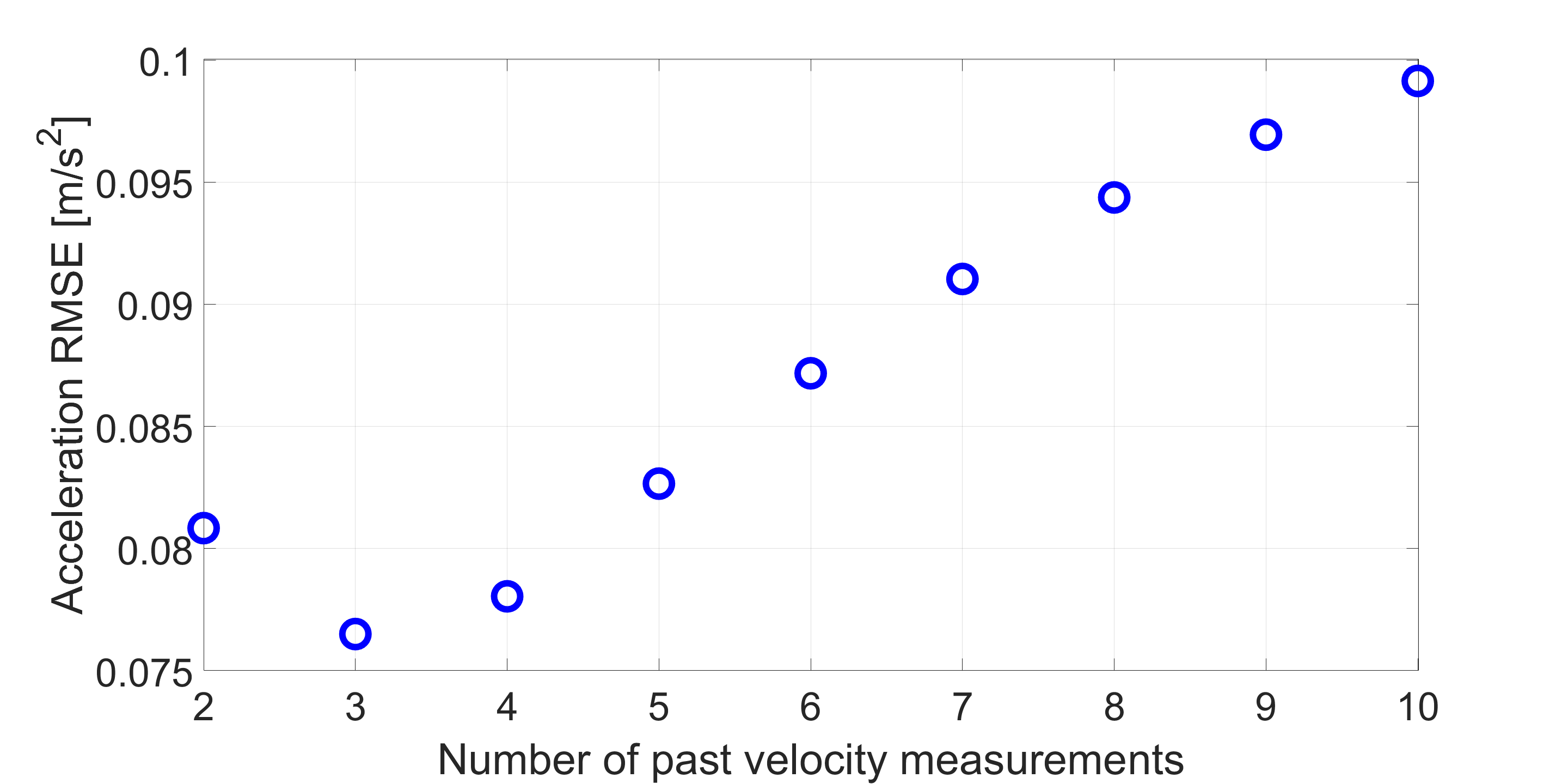
Figure 2: Acceleration RMSE as a function of the number of past DVL velocity measurements used to estimate the acceleration vector.)

IV-B Simulations

The proposed approach was initially evaluated using a simulated trajectory consisting of S-maneuvers (lawn mower trajectory), as shown in Figure 3.
Throughout the trajectory, the AUV maintained an average velocity of 0.6 km per hour, covering a total duration of approximately 25 minutes. The motion pattern involved a sequence of straight-line segments, each lasting 5 minutes (300 seconds), with U-turns placed in between them. Each U-turn had a constant angular rate, yet the angular rate varied between different U-turns. The angular rate ranged from approximately 6 degrees per second in the first U-turn to approximately 15 degrees per second in the last one.

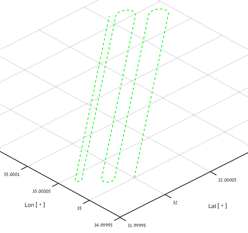
Figure 3: Simulative S-maneuvers (lawn mower trajectory).

Monte Carlo (MC) analysis, consisting of 100 simulations, was conducted, and both velocity and acceleration updates were examined. In the following figures, the blue line represents the estimated standard deviation, obtained as the square root of the estimated covariance. The black line and green line correspond to the standard deviation and mean at each step over the ensemble (MC runs), respectively. A desirable outcome for the MC model is for the estimated and calculated standard deviations to exhibit similar behavior, with the mean over the ensemble being close to zero.
Figure 4 presents the outcomes of the Monte Carlo analyses conducted on the navigation errors observed during the S-maneuvers trajectory. Notably, the velocity errors immediately achieve full convergence due to the direct velocity updates. During the initial 300 seconds, which involve straight-line motion, the misalignment errors of the x-axis and y-axis exhibit slight convergence, while the heading error (z-axis) diverges. However, after the first U-turn, both the x-axis and y-axis misalignment errors promptly converge, and the heading error gradually begins to reduce. Additionally, Figure 5 illustrates the corresponding biases. The dynamics, in this case, lead to full convergence in all accelerometer axes. The x-axis and y-axis gyro biases also converge well, while the z-axis bias converges more slowly.

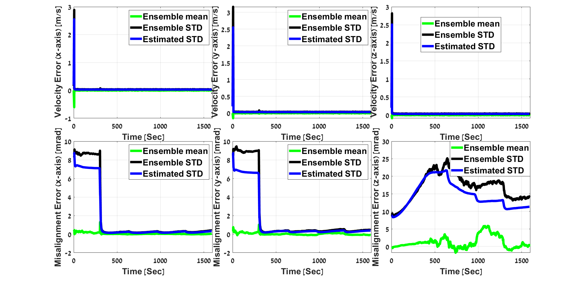
Figure 4: Monte Carlo error-state analysis for the simulative S-maneuvers trajectory.

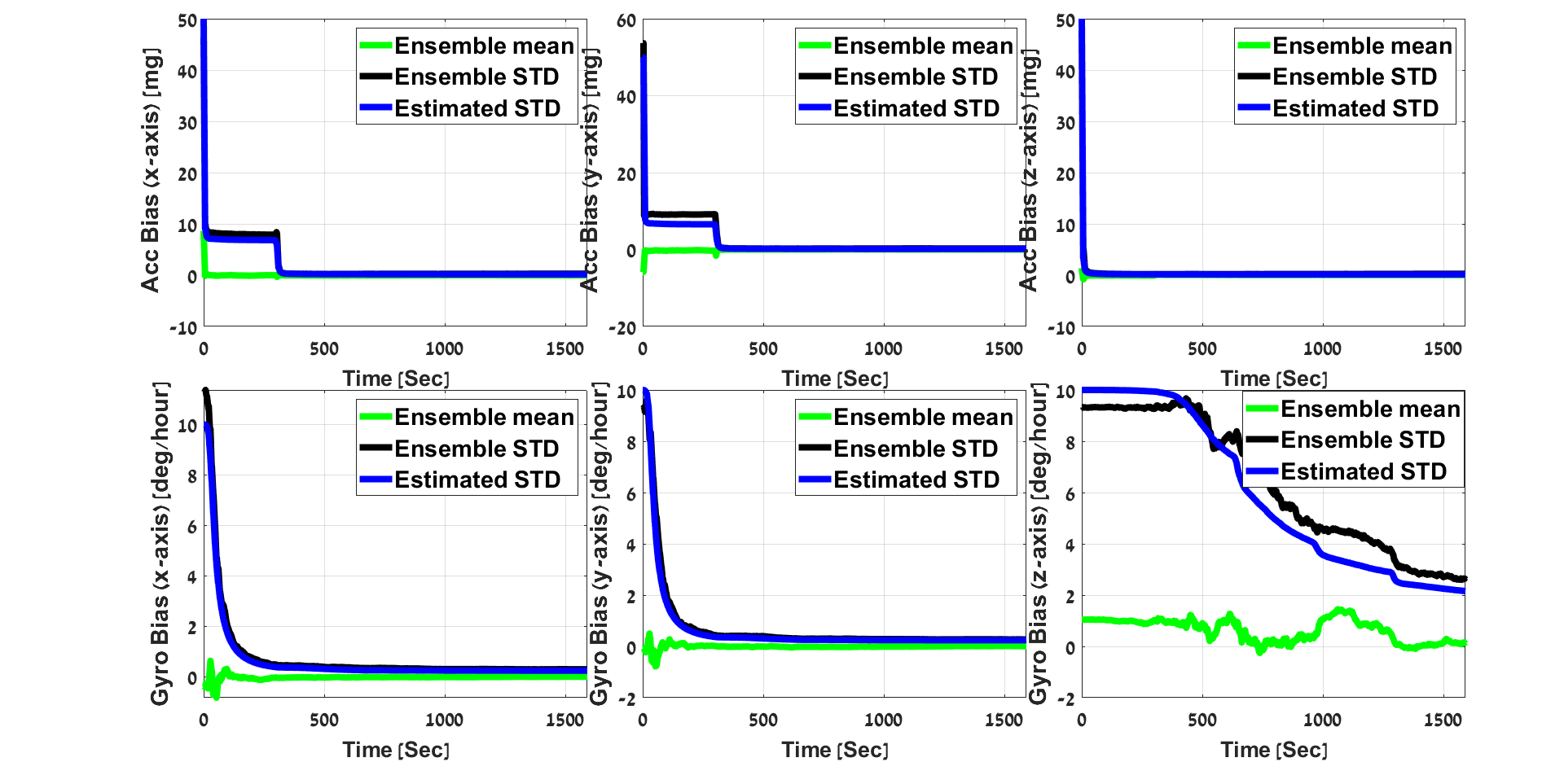
Figure 5: Monte Carlo inertial-state errors analysis for the simulative S-maneuvers trajectory.

It is important to note that the analysis presented in this section pertains specifically to our approach, that is, INS integrated with velocity and acceleration updates. However, we also performed the same analyses on the baseline approach for comparison. Remarkably, the baseline approach yielded the expected results, which further validates the accuracy and reliability of our findings.

IV-C Sea Experiments

To validate our proposed approach, sea experiments were conducted using the Snapir AUV in the Mediterranean Sea. In the following sections, we provide a brief description of the Snapir AUV and present an analysis of the results obtained using the proposed approach and the baseline INS/DVL fusion approach.

IV-C1 Snapir AUV

The Snapir AUV, a modified version of the A18D AUV manufactured by ECA Robotics [24], has been in the possession of the Hatter Department of Marine Technologies at the University of Haifa, Israel since 2017. With a length of 5.5 meters and a weight of 800 kilograms, the AUV is designed for operating at depths of up to 3000 meters. To navigate, it is equipped with a Teledyne RDI Work Horse navigator DVL [25], which can achieve an accuracy of 0.6 cm/s while traveling at a speed of 3 m/s and operating at a frequency of 1 Hz. Figure 6 shows a photograph of the Snapir AUV during the experiment.

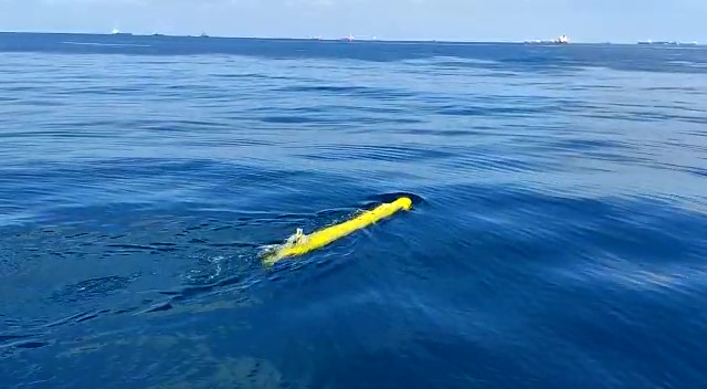
Figure 6: The Snapir AUV navigating at the Mediterranean Sea during the sea experiment near Haifa, Israel.

IV-C2 Trajectories

During the sea experiments, the navigation system data of the Snapir AUV was recorded. We extracted two segments from the recorded data. The first segment corresponds to a straight-line trajectory with a nearly constant velocity of two meters per second during a time period of 424 seconds. The second segment represents a highly dynamic motion, where the AUV performs a figure-of-eight maneuver, maintaining an average velocity of 0.9 meters per second for a duration of 394 seconds. Notably, the AUV exhibited an average angular rate of 1.41 degrees per second, reaching a maximum of 17 degrees per second during the sharp turns of the figure-of-eight maneuver. Figure 7 shows a top view of the figure-of-eight segment.
As a reference (ground truth) we used the Snapir AUV navigation system solution. For both the suggested approach and the baseline INS/DVL, we used the raw IMU and DVL measurements as input.

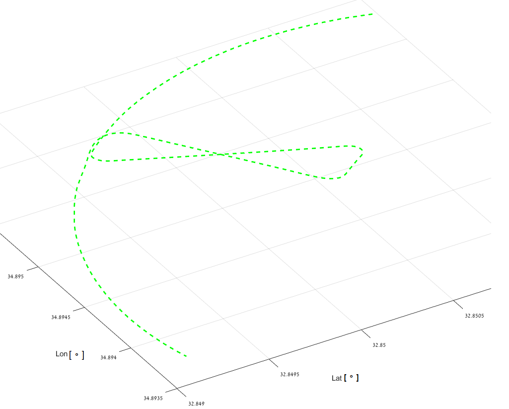
Figure 7: Top view of the eight-figure segment made with the Snapir AUV during experiments at the Mediterranean Sea.

IV-C3 Performance Comparison

In the following figures, we present a comparison between the navigation performance of our approach (in blue) and the baseline INS/DVL fusion (in red) for the two segments tested. The navigation performance is evaluated based on the estimated errors, which are calculated as the square root of the estimated error-state covariance. In addition, we provide two tables for each trajectory to highlight the improvement in accuracy and convergence rate of our proposed approach. As our results show that the estimation of the velocity error-states is similar in both approaches (as directly observed through velocity updates), they are not included in the comparisons.
Figures 8-9 present the results for the straight-line trajectory. In both figures, the numerical results align with our analytical observability analysis, confirming that the addition of acceleration updates does not transform unobservable states into observable ones. The z-axis accelerometer bias, along with the x-axis and y-axis gyro biases, are observable. The x-axis and y-axis (leveling) angle errors are shown to correlate with the estimation of the x-axis and y-axis accelerometer biases. The results indicate a constrained and interrelated estimation of these states, suggesting their close connection in the navigation system.

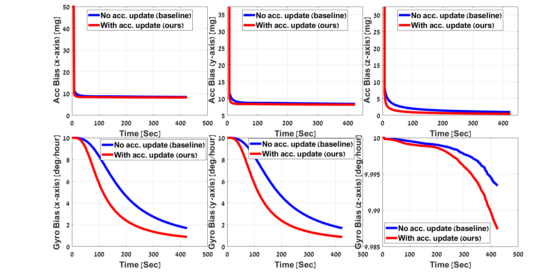
Figure 8: Sea experiment Snapir AUV straight-line trajectory: inertial sensor error-states.

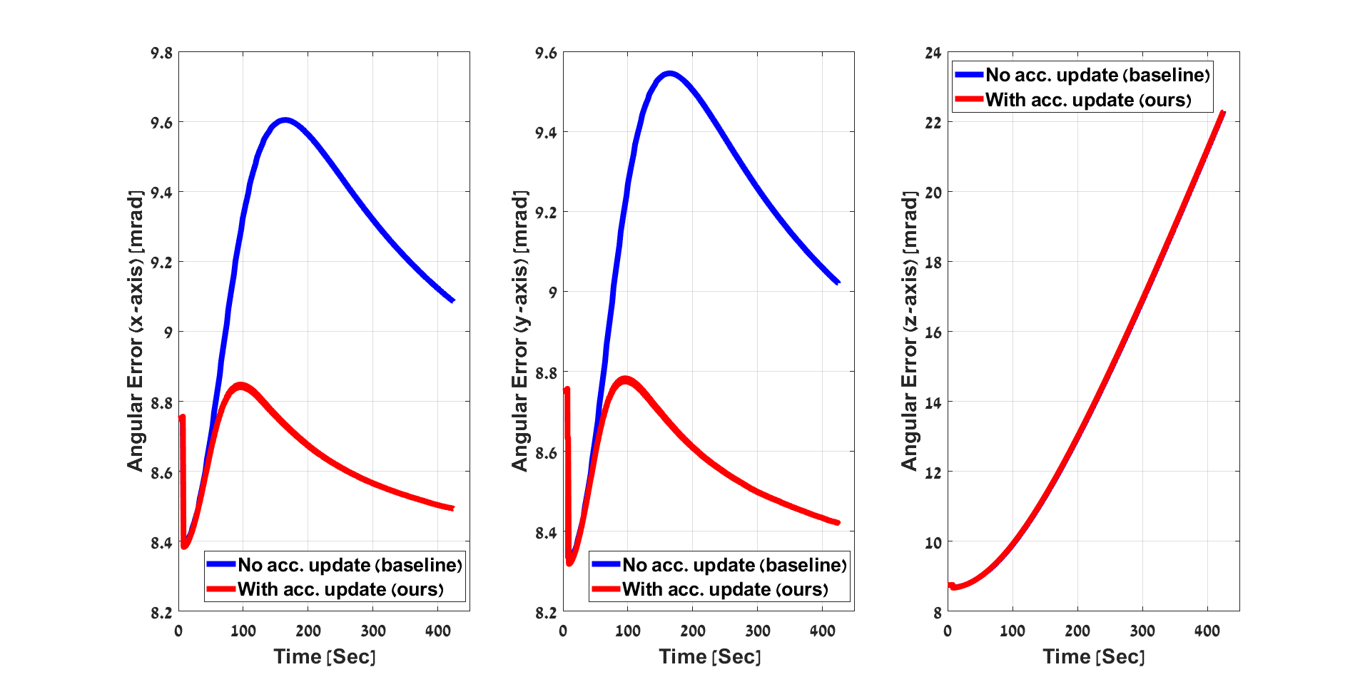
Figure 9: Sea experiment Snapir AUV straight-line trajectory: inertial misalignment error-states.

Yet, despite this similarity in observability, the proposed approach showcases a substantial improvement in navigation performance. Specifically, it significantly reduces the estimation error for the z-axis accelerometer bias by 53%, as well as the estimation errors for the x-axis and y-axis gyro biases by 48%. Moreover, there is an improvement of nearly 7% in the estimation of the leveling angle error.
A comparison of the accuracy in estimating each state at the end of the trajectory for the straight-line trajectory is given in Table I. Our proposed approach demonstrated a substantial improvement in error estimation compared to the baseline approach, with an average enhancement of approximately 19% for misalignment errors and IMU biases in the straight-line segment.

TABLE I: Sea experiment Snapir AUV straight-line trajectory: errors at the end of the trajectory.

State	No Acc. (Baseline)	With Acc. (Ours)	Improvement [%]
$\varphi_{N}$ [mrad]	9.09	8.49	6.60%
$\varphi_{E}$ [mrad]	9.02	8.42	6.65%
$\varphi_{D}$ [mrad]	22.26	22.26	-
$b_{a_{x}}$ [mg]	8.43	8.19	2.85%
$b_{a_{y}}$ [mg]	8.41	8.18	2.73%
$b_{a_{z}}$ [mg]	0.99	0.46	53.54%
$b_{g_{x}}$ [∘/h]	1.69	0.86	49.11%
$b_{g_{y}}$ [∘/h]	1.73	0.91	47.40%
$b_{g_{z}}$ [∘/h]	9.99	9.99	-
Average Improvement			$18.76\%$

Table II provides the time required by our approach to reach the same accuracy level as the baseline approach obtained at the end of the trajectory. The results demonstrate a significantly faster convergence of our approach with an average improvement of approximately 57%. For instance, it took 424 seconds for the baseline approach and only 30 seconds for our approach to reach the same level of accuracy for the x-axis and y-axis accelerometer biases.

TABLE II: Sea experiment Snapir AUV straight-line trajectory: convergence time of our approach to the same level of accuracy the baseline approach provided at the end of the trajectory.

State	Time to reach baseline final performance [sec]	Improvement [%]
$\varphi_{N}$	99	76.65%
$\varphi_{E}$	100	76.42%
$\varphi_{D}$	-	-
$b_{a_{x}}$	31	92.69%
$b_{a_{y}}$	32	92.45%
$b_{a_{z}}$	88	79.25%
$b_{g_{x}}$	256	39.62%
$b_{g_{y}}$	258	39.15%
$b_{g_{z}}$	363	14.39%
Average Improvement		$56.73\%$

The same analysis is made for the eight-figure trajectory. The results of this analysis are presented in Figures 11-10. Figure 11 shows the improved estimation of the leveling angles error-states due to the dynamic nature of the motion pattern in trajectory. Figure 10 demonstrates how the change in orientation that occurs after a 100-second time period enhances the estimation of the x-axis and y-axis accelerometer residuals compared to the straight-line segment. The estimation of the z-axis gyro bias, which is closely linked to the heading error, remains unobservable in the current stage of the analysis.

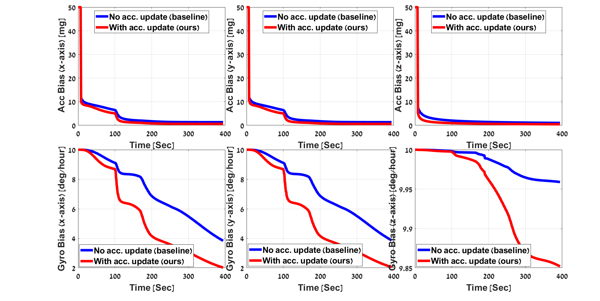
Figure 10: Sea experiment Snapir AUV eight-figure trajectory: inertial sensor error-states.

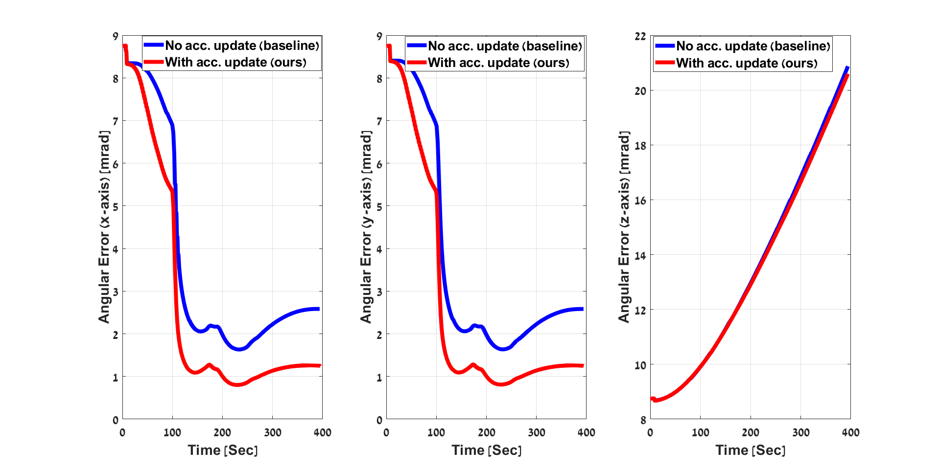
Figure 11: Sea experiment Snapir AUV eight-figure trajectory: inertial misalignment error-states.

A comparative analysis between the proposed approach and the baseline method reveals a substantial improvement in performance. The estimation error of accelerometer biases experiences a significant reduction of 54-55% across all axes, while the estimation error for leveling angles shows a notable improvement of 51%. Table III give the results of this comparison on all error-states.

TABLE III: Sea experiment Snapir AUV eight-figure trajectory: errors at the end of the trajectory.

State	No Acc. (Baseline)	With Acc. (Ours)	Improvement [%]
$\varphi_{N}$ [mrad]	2.58	1.26	51.41%
$\varphi_{E}$ [mrad]	2.61	1.29	50.57%
$\varphi_{D}$ [mrad]	20.87	20.59	1.32%
$b_{a_{x}}$ [mg]	1.34	0.61	54.24%
$b_{a_{y}}$ [mg]	1.41	0.68	51.77%
$b_{a_{z}}$ [mg]	1.02	0.45	55.34%
$b_{g_{x}}$ [∘/h]	3.83	2.02	47.36%
$b_{g_{y}}$ [∘/h]	3.86	2.05	47.01%
$b_{g_{z}}$ [∘/h]	9.96	9.85	1.08%
Average Improvement			$40.01\%$

Table IV provides the convergence time comparison for the eight-figure trajectory, similar to that conducted for the straight-line trajectory. It can be observed that by utilizing the suggested approach, there is an average improvement of 54% in convergence time. Additionally, it is evident that reaching the same overall performance achieved after 394 seconds using the baseline method requires only 225 seconds when employing the suggested approach.

TABLE IV: Sea experiment Snapir AUV eight-figure trajectory: convergence time of our approach to the same level of accuracy the baseline approach provided at the end of the trajectory.

State	Time to reach baseline final performance [sec]	Improvement [%]
$\varphi_{N}$	109	72.34%
$\varphi_{E}$	108	72.59%
$\varphi_{D}$	-	-
$b_{a_{x}}$	134	65.99%
$b_{a_{y}}$	133	66.24%
$b_{a_{z}}$	88	77.66%
$b_{g_{x}}$	225	42.89%
$b_{g_{y}}$	223	43.40%
$b_{g_{z}}$	207	47.46%
Average Improvement		$54.29\%$

V Conclusion

In this study, we proposed an approach to enhance the fusion between the INS and DVL by utilizing DVL-based acceleration measurements. To that end, we derived the acceleration measurement model required in the navigation filter and provided its analytical observability analysis. The observability analysis showed that the additional acceleration measurement does not improve the overall system accuracy. However, as expected, the acceleration measurements improve the accuracy and convergence time of the baseline fusion. This behavior was demonstrated using simulations and sea experiments using the Snapir AUV. Our approach improved the accuracy at the end of the trajectories on all error states by an average improvement of $18\%$ for the straight-line trajectory and $40\%$ for the eight-figure trajectory. Moreover, the proposed approach exhibited significantly faster convergence of the error states to the same level of the baseline accuracy at the end of the trajectory, showing an average improvement of approximately $57\%$ for the straight-line trajectory and $54\%$ for the eight-figure trajectory. Additionally, the proposed approach continued to converge and improve error estimation, leading to even better accuracy over time.
Our proposed approach requires only additional software, making it suitable also for operational AUVs. Also, due to the improved overall performance, our approach has the potential to enable the use of lower-grade sensors. This aspect could lead to the development of simpler low-cost and low-weight navigation systems in small or micro platforms.

References

- [1] P. E. Hagen, N. Storkersen, K. Vestgard, and P. Kartvedt, “The hugin 1000 autonomous underwater vehicle for military applications,” in Oceans 2003. Celebrating the Past… Teaming Toward the Future (IEEE Cat. No. 03CH37492), vol. 2. IEEE, 2003, pp. 1141–1145.
- [2] S.-W. Huang, E. Chen, and J. Guo, “Efficient seafloor classification and submarine cable route design using an autonomous underwater vehicle,” IEEE Journal of Oceanic Engineering, vol. 43, no. 1, pp. 7–18, 2017.
- [3] H. Kondo and T. Ura, “Navigation of an AUV for investigation of underwater structures,” Control Engineering Practice, vol. 12, no. 12, pp. 1551–1559, 2004.
- [4] J. Bao, D. Li, X. Qiao, and T. Rauschenbach, “Integrated navigation for autonomous underwater vehicles in aquaculture: A review,” Information Processing in Agriculture, vol. 7, no. 1, pp. 139–151, 2020.
- [5] B. Barshan and H. F. Durrant-Whyte, “Inertial navigation systems for mobile robots,” IEEE Transactions on Robotics and Automation, vol. 11, no. 3, pp. 328–342, 1995.
- [6] L. Stutters, H. Liu, C. Tiltman, and D. J. Brown, “Navigation technologies for autonomous underwater vehicles,” IEEE Transactions on Systems, Man, and Cybernetics, Part C (Applications and Reviews), vol. 38, no. 4, pp. 581–589, 2008.
- [7] D. Titterton and J. Weston, “Strapdown inertial navigation,” London: Peter Peregrinus Ltd, 1997.
- [8] P.-M. Lee and B.-H. Jun, “Pseudo long base line navigation algorithm for underwater vehicles with inertial sensors and two acoustic range measurements,” Ocean Engineering, vol. 34, no. 3-4, pp. 416–425, 2007.
- [9] H. Rice, S. Kelmenson, and L. Mendelsohn, “Geophysical navigation technologies and applications,” in PLANS 2004. Position Location and Navigation Symposium (IEEE Cat. No. 04CH37556). IEEE, 2004, pp. 618–624.
- [10] L. Paull, S. Saeedi, M. Seto, and H. Li, “AUV navigation and localization: A review,” IEEE Journal of Oceanic Engineering, vol. 39, no. 1, pp. 131–149, 2013.
- [11] Y. Geng, R. Martins, and J. Sousa, “Accuracy analysis of DVL/IMU/magnetometer integrated navigation system using different IMUs in AUV,” in IEEE ICCA 2010. IEEE, 2010, pp. 516–521.
- [12] P. A. Miller, J. A. Farrell, Y. Zhao, and V. Djapic, “Autonomous underwater vehicle navigation,” IEEE Journal of Oceanic Engineering, vol. 35, no. 3, pp. 663–678, 2010.
- [13] P. J. B. Sánchez, M. Papaelias, and F. P. G. Márquez, “Autonomous underwater vehicles: Instrumentation and measurements,” IEEE Instrumentation & Measurement Magazine, vol. 23, no. 2, pp. 105–114, 2020.
- [14] A. Tal, I. Klein, and R. Katz, “Inertial navigation system/doppler velocity log (INS/DVL) fusion with partial DVL measurements,” Sensors, vol. 17, no. 2, p. 415, 2017.
- [15] P. Liu, B. Wang, Z. Deng, and M. Fu, “INS/DVL/PS tightly coupled underwater navigation method with limited DVL measurements,” IEEE Sensors Journal, vol. 18, no. 7, pp. 2994–3002, 2018.
- [16] I. Klein and Y. Lipman, “Continuous INS/DVL fusion in situations of DVL outages,” in 2020 IEEE/OES Autonomous Underwater Vehicles Symposium (AUV). IEEE, 2020, pp. 1–6.
- [17] B. Braginsky, A. Baruch, and H. Guterman, “Correction of DVL error caused by seafloor gradient,” IEEE Sensors Journal, vol. 20, no. 19, pp. 11 652–11 659, 2020.
- [18] I. Klein, Y. Gutnik, and Y. Lipman, “Estimating DVL velocity in complete beam measurement outage scenarios,” IEEE Sensors Journal, vol. 22, no. 21, pp. 20 730–20 737, 2022.
- [19] P. Groves, “Principles of GNSS, inertial, and multisensor integrated navigation systems, 2nd edn. GNSS/GPS. Artech House,” 2013.
- [20] J. Farrell, Aided Navigation: GPS with High Rate Sensors. McGraw-Hill, Inc., 2008.
- [21] P. Maybeck, Stochastic Models, Estimation and Control. New York, NY, USA: Academic Press, 1982.
- [22] I. Klein and R. Diamant, “Observability analysis of DVL/PS aided INS for a maneuvering AUV,” Sensors, vol. 15, no. 10, pp. 26 818–26 837, 2015.
- [23] ——, “Observability analysis of heading aided INS for a maneuvering AUV,” NAVIGATION: Journal of the Institute of Navigation, vol. 65, no. 1, pp. 73–82, 2018.
- [24] E. Robotics, “ECA robotics @online,” Available: https://www.ecagroup.com/en/solutions/a18-d-auv-autonomous-underwater-vehicle, Accessed on: June 2023.
- [25] T. Marine, “Teledyne Marine @online,” Available: http://www.teledynemarine.com/dvls, Accessed on: June 2023.