A General Framework for Progressive Data Compression and Retrieval

Abstract

In scientific simulations, observations, and experiments, the cost of transferring data to and from disk and across networks has become a significant bottleneck that particularly impacts subsequent data analysis and visualization. To address this challenge, compression techniques have been widely adopted. However, traditional lossy compression approaches often require setting error tolerances conservatively to respect the numerical sensitivities of a wide variety of post hoc data analyses, some of which may not even be known a priori. Progressive data compression and retrieval has emerged as a solution, allowing for the adaptive handling of compressed data according to the needs of a given post-processing task. However, few analysis algorithms natively support progressive data processing, and adapting compression techniques, file formats, client/server frameworks, and APIs to support progressivity can be challenging. This work presents a general framework that supports progressive-precision data queries independently of the underlying data compressor or number representation. Our approach is based on a multiple-component representation that successively, with each new component, reduces the error between the original and compressed field, allowing each field in the progressive sequence to be expressed as a partial sum of components. We have implemented our approach on top of four popular scientific data compressors and have evaluated its behavior on several real-world data sets from the SDRBench collection. Numerical results indicate that our framework is effective in terms of accuracy compared to each of the standalone compressors it builds upon. In addition, compression and decompression time are proportional to the number and granularity of components, as requested by the user. Finally, our framework allows for fully lossless compression using lossy compressors when a sufficient number of components are employed.

Introduction

With the arrival of the exascale era in high-performance computing, achieving efficient hardware utilization is no longer solely dependent on compute power. Instead, one needs to account for the cost of data movement between various components of a computer system, such as DRAM and registers, CPU cores and accelerators, distributed compute nodes, and main memory and offline storage. It is not practical to record every byte produced in scientific observations, experiments, and simulations, so data must be reduced using compression methods that eliminate redundancy and bits of marginal accuracy in floating-point arrays.

To address this challenge, numerous lossy compressors for floating-point data have been developed in recent years, including mgard [1], sperr [30], sz [33], and zfp [34], to name a few. These compressors are typically inserted at select points in the memory hierarchy, usually near offline storage, and compression parameters are set for a specific use case, such as checkpointing, data analysis, or visualization. In this context, decompressing data for subsequent processing generally requires the transfer and decompression of whole fields, which incurs expensive data movement and (at least temporary) storage costs that compression techniques were designed to alleviate. Furthermore, the output of a single simulation, observation, or experiment may feed into multiple analyses with varying requirements in resolution, precision, and regions of interest in space and time.

The data thus obtained at great expense is often shared across facilities, e.g., via community databases, to benefit the community at large, allowing both intended and unforeseen scientific studies to be carried out—a few example domains include climate [28, 14], astronomy [50], particle physics [41], and turbulence [19]. Faced with a diversity of application domains and use cases with varying requirements on data fidelity (e.g., precision and resolution), lossy compression—when integrated—is often used conservatively to cater to the least common denominator of known or anticipated accuracy needs. This “one-size-fits-all” approach can waste resources, especially for downstream data analysis applications that do not require or even benefit from extraneous precision or resolution, yet must query and transfer full-fidelity data from a central repository.

One proposed solution to combat the high cost of data transfer is to use progressive compression that allows extracting reduced-fidelity data with a smaller compressed storage and transfer cost [10, 32, 9, 25, 6]. This allows the data to be archived at or near full fidelity, with each client (data consumer) specifying its fidelity needs so that only as much compressed data as necessary is transferred. Usually, a progressive representation also allows incrementally refining an approximation of the data as more compressed data arrives. Unfortunately, while ubiquitous for image transmission over the web, few scientific databases make use of progressive compression for several reasons:

• Popular file formats and I/O libraries like HDF5 [15], NetCDF [42], ADIOS [17], and ROOT [2], while supporting compression, do not come with progressive-access support. Hence, one must forego such tools and instead rely on custom file formats and I/O libraries.

• Few compressors intrinsically support progressive access, with mgard [1] and vapor [29] being notable exceptions rather than the norm.

• Even though compressors based on wavelets (for progressive resolution) or bit plane coding (for progressive precision) could be made to support progressive access, the engineering and implementation challenges can be substantial. Moreover, the (de)compressor API and implementation must be modified to support such queries, and usually a specialized client/server layer is needed to coordinate the transfer and integration of data that will ultimately be served to the science application requesting it.

In this paper, we advocate for a much simpler but pragmatic approach to progressive-precision queries that supports any lossy compressor or number representation without the need for invasive code changes or custom file format. Our framework is based on the idea of multi-component decomposition—well-known in fields like multiple-precision arithmetic, with double-double [24] being perhaps the best-known representation—but generalizes the use of a vector of low-precision floating-point numbers to represent a high-precision scalar by building on top of lossy numerical compression. The salient aspects of our framework are:

• A multi-dimensional scalar field is expressed as a sum of components with (typically) exponentially increasing accuracy. Each component represents the remaining error from the partial sum of components preceding it, and is compressed independently by a lossy compressor of the user’s choosing.

• We require no special file format, API, or client/server framework. Rather, the components constitute an additional data dimension, with the convention that the consumer requests a subset of compressed components that are decompressed and added to form an approximation. Existing compression plugins for formats like HDF5 can thus be reused as is.

• Incremental refinement is supported trivially by simply “adding in” components to the reconstruction as they arrive. Hence, no additional decompressor state or previously received compressed data needs to be buffered.

• Our approach supports error tolerances, with the application requesting only as many components as needed to satisfy its accuracy requirements. In the limit, we can ensure lossless compression via lossy compressors if desired.

• The granularity of progressivity can be chosen by both the data producer and, later, by the data consumer in terms of the total number of components stored or number of components consumed together. Usually, there is a tradeoff between granularity supported and overhead in storage and compute time.

We detail our approach after reviewing related work on progressive compression of numerical data.

1 Related Work

In this section, we review related work on progressive compression in the context of scientific data. In particular, we limit the discussion to multidimensional scalar fields defined on structured grids. For a more general discussion of lossy compression and unstructured data, we refer the reader to the recent survey of Li et al. [31].

Progressive representations allow the reconstruction of a field by decompressing only a subset of the compressed bit stream and by incrementally refining the reconstruction as additional compressed bits are processed. Usually, the bit stream is organized such that early bits have the most impact on accuracy and such that any prefix of the bit stream gives near-optimal quality at that given bit rate. There are currently two dominant approaches: progression in resolution (in space, time, or both), usually with low-frequency components transmitted first, and progression in precision, where the most significant bits are processed first.

In the former camp, numerous multiresolution hierarchies have been proposed, including those based on subsampling [39], spectral transformations like the Fourier and discrete cosine transform [52], Laplacian pyramids [7], wavelets and related sub-band decompositions [29, 30, 1], as well as rank decompositions like SVD and HOSVD [4, 3], which tend to generate basis functions that loosely correspond to frequency. Oftentimes such representations support progression by simply thresholding or truncating basis coefficients, essentially performing a form of low-pass filtering, with subsequent coefficients introducing higher-frequency details.

Whereas in the first camp, some subset of coefficients are encoded at full precision, approaches in the second camp are typified by encoding some subset of “bit planes” (the set of bits with the same place value) for all coefficients, from most to least significant bit. Examples originally developed for wavelet-based image compression include embedded zerotree wavelet (ezw) coding [47], set partitioning in hierarchical trees (spiht) [43], and variants such as set partitioned embedded block (speck) [40]. These techniques capitalize on the sparsity of wavelet coefficients, which are often small with many leading zeros that can be encoded efficiently together. Using the idea of group testing [27], many bits are pooled, tested together, and then iteratively refined if the group contains at least one one-bit. Such techniques have been adopted in scientific data compressors like zfp [34] and sperr [30], though without direct support for progressive reconstruction. Also, recognizing that many zero-bits tend to occur together, long runs of zeros may be encoded using run-length encoding (RLE), as in the tthresh compressor [4].

We note that embedded coders like ezw and spiht are generally presented not in terms of encoding bit planes but rather as encoding comparisons of coefficient magnitudes with a decreasing sequence of thresholds, $\tau_{1}>\tau_{2}>\tau_{3}\cdots$. A coefficient exceeding such a threshold is deemed significant. Once a coefficient has been found to be significant, its less-significant bits are coded in subsequent passes separate from the significance tests. When $\tau$ is an integer power of two, as is typically the case, this approach reduces to bit plane coding. Our progressive framework also is based on a sequence of thresholds or error tolerances, though not necessarily consecutive integer powers of two.

Recognizing that these two camps represent two extremes—either encode full precision for a subset of coefficients or encode all coefficients at the same precision—Hoang et al. [25, 26] recently proposed exploring both dimensions of progression simultaneously, thus providing flexibility in trading precision and resolution tailored to the task at hand. An alternative representation with similar capabilities was more recently proposed [6], with less fine-grained progression in precision. With recent additions to mgard [1], one may similarly refine in precision or resolution [32, 18]. Likewise, wavelet-based image compressors such as JPEG2000 [9] organize bit streams to support refinement in both resolution and precision. Through the remainder of this paper, however, we restrict our discussion to progression in precision.

We note that the progressive techniques discussed here—especially those that support progression in both precision and resolution—require additional data structures to maintain not only the current approximation in the progression but also sufficient information to allow refining that approximation—i.e., the current “cut”—represented for example as hash maps of grid points [6] or partial wavelet sub-bands [26]. This auxiliary information may also include partial state, such as which coefficients are significant [47, 43, 26], to allow the decompressor to know how to interpret the next sequence of bits once they arrive. Moreover, custom file formats are needed that support indexing for random access to small chunks of data [26], and possibly precomputed error matrices [32] that capture the errors resulting from any given combination of resolution and precision. We avoid this additional complexity by decoupling the components that serve as units of refinement, which are (de)compressed independently using an error-bounded compressor.

We conclude this section by referencing the inspiration behind our progressive framework: multi-component representations [12, 48, 24]. Originally developed as a means to extend floating-point precision beyond hardware-supported types, a multi-component representation uses a vector of low-precision numbers to approximate a higher-precision number, wherein each vector component represents the remaining rounding error in the approximation associated with the sum of previous components (see the subsequent section for details). The same principle also underpins the family of iterative refinement methods for linear solvers [51], where one solves not just for a single vector but also a hierarchy of error vectors to boost accuracy, as well as the recently proposed hire algorithm [5], which targets progression in resolution. To our knowledge, our approach is the first to generalize these ideas from multi-component floating-point representation for high-precision arithmetic to the field of lossy data compression.

2 Preliminaries

Before describing our approach, we review the idea behind multi-component representations that underpin it. The key idea is to represent a high-precision number using a vector of lower-precision components, with each additional component capturing the rounding error achieved so far in the sum—computed at full precision—of prior components. In this manner, a double-precision number with 53 mantissa bits can be well-approximated as two single-precision numbers with 24-bit mantissas by effectively concatenating their mantissas. However, note that single precision has smaller dynamic range, limiting the domain of values that can be represented this way.

Let $\mathrm{fl}(\cdot)$ represent the operator that rounds its argument to the nearest low-precision floating-point number. Given a high-precision number, $x$, we define the first component as $x_{1}=\mathrm{fl}(x)$. This results in a rounding error $e=x-x_{1}$, which is captured in a second component: $x_{2}=\mathrm{fl}(e)=\mathrm{fl}(x-x_{1})$ such that $x\approx x_{1}+x_{2}$, where the addition is computed in full precision (the precision used for $x$). Note that this holds only approximately since there is also a secondary rounding error in the computation of $x_{2}$. If equality is not achieved, a third component may be introduced: $x_{3}=\mathrm{fl}(x-(x_{1}+x_{2}))$, and so on, with $x\approx\sum_{i}x_{i}$ and $x_{k}=\mathrm{fl}(x-\sum_{i=0}^{k-1}x_{i})$. By convention, $x_{0}=0$. Note that because floating-point addition is not guaranteed associative, the order in which components are added matters. For consistency, terms are added eagerly from left to right, with each additional component appended to the previous sum: $\tilde{x}_{k+1}=\tilde{x}_{k}+x_{k+1}=\bigl{(}\sum_{i=0}^{k}x_{i}\bigr{)}+x_{k+1}$. Since $x_{k+1}=\mathrm{fl}(x-\tilde{x}_{k})$, $|x_{k+1}|\approx|x-\tilde{x}_{k}|$ represents an estimate (accurate to machine epsilon) of the error in using $\tilde{x}_{k}$ to approximate $x$.

3 Multi-Component Representation

Equipped with a multi-component construction algorithm for scalars based on conventional floating point, we now generalize this approach to scalar fields, $\mathbf{x}$, stored in other number representations. In place of $\mathrm{fl}(\cdot)$, we rely on lossy compression, $\mathbb{C}(\cdot)$, and decompression, $\mathbb{D}(\cdot)$, functions, with the composition $\mathbb{D}\circ\mathbb{C}$ taking on the role previously held by $\mathrm{fl}(\cdot)$ to approximate the input using reduced precision. Any lossy compression algorithm takes some parameter that governs the amount of loss. This could, for instance, be a target bit rate that directly controls the amount of compressed storage [34], a target error under some chosen norm, like $L_{2}$ [4], or an error tolerance, $\tau$, that bounds the pointwise maximum absolute difference between the uncompressed and lossy-compressed fields, as supported by most contemporary compressors [1, 30, 33, 34]. We will present our framework in terms of a decreasing sequence of such absolute error tolerances, $\tau_{1}>\tau_{2}>\cdots>\tau_{n}$, while noting that other compression parameters can easily be substituted.

3.1 Progressive Compression

Algorithm 1 Multi-component data compression

0:  $\mathbf{x};\,n;\,\mathbb{C}(\mathbf{x},\tau);\,\mathbb{D}(\mathbf{y});\,(\tau_{1},\tau_{2},\ldots,\tau_{n}):\tau_{i}>\tau_{i+1}$

0:  $(\mathbf{y}_{1},\mathbf{y}_{2},\ldots,\mathbf{y}_{n})$

1:  $\tilde{\mathbf{x}}\leftarrow\mathbf{0}$

2:  for $i\leftarrow 1,\ldots,n$ do

3:     $\mathbf{e}\leftarrow\mathbf{x}-\tilde{\mathbf{x}}$

4:     $\mathbf{y}_{i}\leftarrow\mathbb{C}(\mathbf{e},\tau_{i})$

5:     $\mathbf{x}_{i}\leftarrow\mathbb{D}(\mathbf{y}_{i})$

6:     $\tilde{\mathbf{x}}\leftarrow\tilde{\mathbf{x}}+\mathbf{x}_{i}$

7:  end for

Algorithm 1 details our multi-component construction method. The method takes as input the desired number of components, $n$, the original (uncompressed) data as a vector of double-precision floating-point values, $\mathbf{x}$, and the aforementioned sequence of decreasing error tolerances, $(\tau_{1},\tau_{2},\ldots,\tau_{n})$, selected by the user. For the sake of simplicity, we omit other input parameters that are needed by the compressor such as the grid dimensions of the uncompressed field. On Line 1, the current approximation, $\tilde{\mathbf{x}}$, to $\mathbf{x}$ is initialized to a field of all zeros. Next, we loop over the components, $\mathbf{x}_{i}$, to be constructed. In each iteration, we compute the current error $\mathbf{e}=\mathbf{x}-\tilde{\mathbf{x}}$, which decreases with each iteration. $\mathbf{e}$ is then compressed to within a tolerance, $\tau_{i}$, forming the $i^{\text{th}}$ compressed component, $\mathbf{y}_{i}$. We then immediately decompress $\mathbf{y}_{i}$, yielding $\mathbf{x}_{i}$. Given the imposed error tolerance, we are thus assured that $\|\mathbf{e}-\mathbf{x}_{i}\|_{\infty}\leq\tau_{i}$. Finally, we update $\tilde{\mathbf{x}}$ by adding in the just computed component, $\mathbf{x}_{i}$, resulting in a more accurate approximation. The output of the algorithm is the sequence of compressed components, $(\mathbf{y}_{1},\mathbf{y}_{2},\ldots,\mathbf{y}_{n})$.

3.2 Progressive Reconstruction

Algorithm 2 Multi-component data reconstruction

0:  $m\leq n;\,\mathbb{D}(\mathbf{y});\,(\mathbf{y}_{1},\mathbf{y}_{2},\ldots,\mathbf{y}_{n})$

0:  $\tilde{\mathbf{x}}$

1:  $\tilde{\mathbf{x}}\leftarrow\mathbf{0}$

2:  for $i\leftarrow 1,\ldots,m$ do

3:     $\mathbf{x}_{i}\leftarrow\mathbb{D}(\mathbf{y}_{i})$

4:     $\tilde{\mathbf{x}}\leftarrow\tilde{\mathbf{x}}+\mathbf{x}_{i}$

5:  end for

A progressive reconstruction based on a subset of $m\leq n$ components is obtained by executing Algorithm 2. This algorithm is essentially the same as Algorithm 1 but with Lines 3–4, which compute and compress the error, excluded, and with the loop on Line 2 shortened to $m$ iterations. We note that we can trivially continue refining the reconstruction, $\tilde{\mathbf{x}}$, by incorporating additional components as they arrive by simply executing additional loop iterations.

3.3 Error Bounds

The sequence of error tolerances utilized by our construction algorithm serves not only to induce a sequence of approximations but also as (approximate) error bounds in the resulting reconstructions $\{\tilde{\mathbf{x}}_{i}\}$. To see why this is, let $\mathbf{e}_{i}=\mathbf{x}-\tilde{\mathbf{x}}_{i-1}$. As the single-component compressor $\mathbb{C}$ ensures $\|\mathbf{e}_{i}-\mathbf{x}_{i}\|_{\infty}\leq\tau_{i}$, we have

$$\begin{split}\|\mathbf{x}-\tilde{\mathbf{x}}_{i}\|_{\infty}&=\|\mathbf{x}-(\tilde{\mathbf{x}}_{i-1}+\mathbf{x}_{i})\|_{\infty}\\ &=\|(\mathbf{x}-\tilde{\mathbf{x}}_{i-1})-\mathbf{x}_{i}\|_{\infty}=\|\mathbf{e}_{i}-\mathbf{x}_{i}\|_{\infty}\leq\tau_{i}.\end{split}$$ (1)

However, we here rely on the use of the associative rule $\mathbf{x}-(\tilde{\mathbf{x}}_{i-1}+\mathbf{x}_{i})=(\mathbf{x}-\tilde{\mathbf{x}}_{i-1})-\mathbf{x}_{i}$, which does not necessarily hold as computations are being performed in floating-point arithmetic, i.e., this bound may be violated by a small constant proportional to machine epsilon. This is in practice of little consequence as $\mathbf{x}$ already is contaminated by similar rounding errors, which in turn are often dwarfed by larger sensor, truncation, iteration, and model errors.

In case the underlying compressor is not driven by an absolute error tolerance but by some other compression parameter, we advocate computing the corresponding errors, i.e., set $\tau_{i}\leftarrow\|\mathbf{x}-\tilde{\mathbf{x}}_{i}\|_{\infty}$ and maintain $\{\tau_{i}\}$ as additional metadata for later use in specifying the required accuracy. One may even choose to do so with error-bounded compressors that provide only a loose error bound, like mgard and zfp, to further tighten the error bounds.

3.4 Compressibility of Components

We note that in each iteration of our algorithm, we are compressing the remaining error, $e_{i}$, in the approximation. As $i$ increases, these errors tend to become increasingly random as any spatial correlation (or “smoothness”) in the data is lost. Such randomness is usually a bane for numerical compressors, and we would expect compression to become increasingly less effective. Worse yet, due to the pigeonhole principle, some inputs to a compressor must lead to expansion, so it is legitimate to question the efficacy of our approach.

We make two points in defense of our framework: (1) Whether one compresses a data set in batches using multiple components or in a single sweep, the same high-entropy less-significant bits that are still needed to attain a certain level of accuracy must be faithfully preserved. In a conventional single-component compressor, such trailing bits are either encoded verbatim explicitly, as in [34, 43, 40, 30], or implicitly, e.g., using Huffman codes [33]. In a multi-component compressor, groups of consecutive bit planes are effectively isolated and compressed independently, however this in and of itself does not significantly impact the compressibility of said bits. Rather, the main penalty in using a multi-component representation lies in the per-component overhead one may expect, e.g., zfp encodes one exponent per block and component; sz embeds a Huffman table with each component; and sperr encodes a significance map with each component. However, as we shall see, compressing the data in batches (components) can also improve both compression and error. (2) As precision increases, the magnitude of components decreases, until eventually many values are exactly represented with zero error. As components (i.e., errors) become increasingly sparse, they also become more compressible. We will evaluate the effects that randomness plays in the following section.

4 Numerical Results

In this section, we evaluate our multi-component approach using real-world data fields, primarily from SDRBench [53]; see Table 1. We use four state-of-the-art error-bounded lossy compressors (see Table 2) within the context of our framework, representing a range of different compression techniques:

• zfp is a block-transform-based compressor (similar to JPEG) that uses custom bit plane coding.

• sz encodes corrections to predictions that violate the error tolerance using Huffman coding.

• sperr is based on CDF 9/7 wavelets. Like sz, it encodes corrections to outliers, however using speck.

• mgard uses a custom multilevel basis akin to CDF 5/3 wavelets, coupled with quantization and lossless compression.

We conducted the numerical experiments on a workstation equipped with 64 GB of RAM and an Intel Xeon E5-1650v4 CPU. All source codes were compiled with GCC 12.2.1 and the optimization flags -O3 -march=native. We note that many of the data compressors tested in this work have support for multi-threading or GPU acceleration. However, we decided to test only the single-core CPU execution mode to simplify our analysis.

Table 1: Data sets used to benchmark our approach.

Name	Application type	Dimensions			Precision
Miranda	Hydrodynamics	384 $\times$	384 $\times$	256	64
S3D	Combustion	500 $\times$	500 $\times$	500	64
S3D JICF [20]	Combustion	400 $\times$	250 $\times$	200	64
Nyx	Cosmology	512 $\times$	512 $\times$	512	32
QMCPACK	Quantum chemistry	69 $\times$	69 $\times$	115	32
SCALE	Weather	1200 $\times$	1200 $\times$	98	32

Table 2: Compressors used in our multi-component framework (top) and compared against (bottom).

Compressor	Version/Hash	GitHub repository
zfp [34]	$1.0.0$	LLNL/zfp
sz3 [33]	$3.1.7$	szcompressor/SZ3
sperr [30]	$0.6.2$	NCAR/SPERR
mgard [1]	$28d738c$	lxAltria/MGARDx
idx2 [26]	$4f072cb$	sci-visus/idx2
pmgard [32]	$e581794$	lxAltria/Multiprecision-data-refactoring
fpzip [36]	$1.3.0$	LLNL/fpzip

4.1 Error Analysis

We begin by evaluating the rate-distortion associated with the four compressors discussed above when (1) used in isolation, which we will refer to as “single-component compressors,” and when (2) incorporated into our multi-component framework. Toward this end, we used a sequence of absolute error tolerances, $\tau_{i}=2^{-\Delta\times i}\tau_{0}$, during compression, with $\tau_{0}$ representing the range of field values and $\Delta\in\{4,6,8\}$ being the granularity of progression, in essence governing the precision associated with each component. We used $\Delta=2$ with the single-component compressors and reran them from scratch to obtain a data point for each corresponding error tolerance.

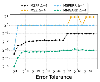
Figure 1: Ratio of observed maximum absolute error to error tolerance, $\tau$, as a function of $\tau$, for the single-component compressors (left) and for $m$-component ($1\leq m\leq n$) reconstructions based on zfp, sz, sperr, and mgard (right). Note that the observed errors generally respect the tolerance, either exactly, by coinciding with the tolerance (ratio equals $2^{0}=1$), or conservatively, by falling below the tolerance. See the text for a discussion of the mgard and zfp plots.

To verify that our framework meets error bounds, we plot in Fig. 1 for the Miranda pressure field the ratio between the measured maximum absolute error and the tolerance, $\tau$, requested during progressive reconstruction, as a function of $\tau$. We note that the multi-component compressors, prefixed with an ‘M’ and suffixed with $\Delta$ in these plots, generally respect the tolerance as this ratio tends to be at or below one. The only exception is msz, which at very small (relative) tolerances below machine epsilon ($2^{-52}$) occasionally gives a 1-ulp (unit in the last place) rounding error due to the non-associativity of floating-point arithmetic, as discussed in Section 3.3. The single-component compressors (no prefix) also respect the tolerance, except for zfp (a known limitation [13, §4.2]) and mgard (as reported elsewhere [30, §VI.C]) when $\tau$ is near machine epsilon. Note that mzfp and mmgard, our multi-component variants, overcome this limitation.

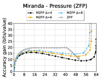
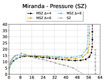
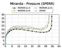
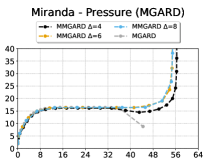
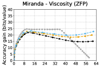
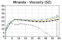
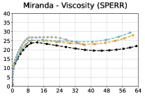
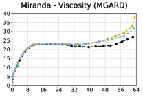
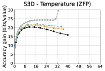
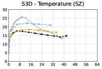
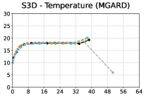
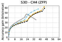
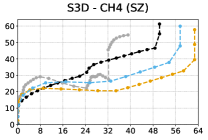
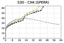
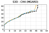
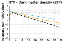
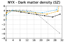
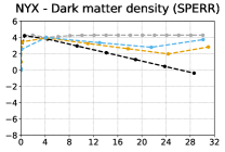
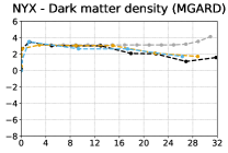
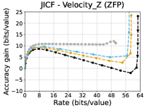
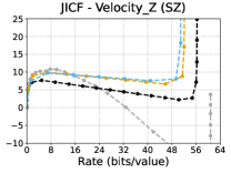
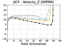
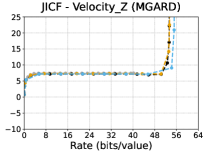
Figure 2: Accuracy gain (higher is better) vs. rate for multi-component approaches based on, from left to right, zfp, sz, sperr, and mgard.

4.1.1 Comparison with Nonprogressive Compressors

For the remaining analysis, our chosen error metric is the recently proposed accuracy gain [35, 30],

$$\alpha=\log_{2}\frac{\sigma}{E}-R,$$ (2)

where $\sigma$ is the standard deviation of the input data, $E$ is the root-mean-square error, and $R$ is the rate in compressed bits per scalar value. $\alpha$ is related to signal-to-noise-ratio ($\mathit{SNR}$, in $\text{dB}/(\text{bit}/\text{value})$) by $\alpha=\frac{\mathit{SNR}}{20\log_{10}2}-R\approx\frac{\mathit{SNR}}{6.02}-R$.

We plot $\alpha(R)$, where a positive slope indicates that, at rate $R$, compression is occurring (more bits of precision are consumed than are output); a negative slope indicates expansion at that rate (more bits are output than are consumed). A flat curve implies that each bit emitted corresponds to one bit of precision consumed, as indicated by a halving of the error, $E$. This type of information is difficult to infer in an $\mathit{SNR}$ plot. We further note that $\alpha$, unlike $\mathit{SNR}$, accounts for both error and rate—hence, an $\alpha$ value on its own is meaningful. Except when approaching lossless compression, where $E\rightarrow 0$ and $\alpha\rightarrow\infty$, $\alpha$ indicates the cumulative number of bits per value that have been inferred by the compressor.

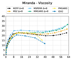
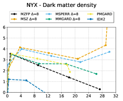
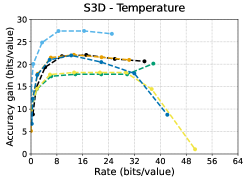
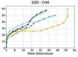
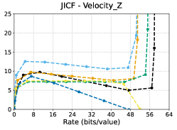
Figure 3: Accuracy gain (higher is better) comparison among our multi-component compressors and with idx2 and pmgard.

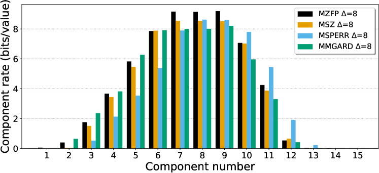
Figure 4: Per-component rate, $R_{i}$, for the Miranda pressure field. Components with $R_{i}>\Delta=8$ expand rather than compress due to high entropy.

Figure 2 shows accuracy gain plots for six data sets using our four single- and multi-component compressors. We note several general trends. First, the single-component compressors (gray curves) often—but not always—do better, especially at low rates. We point out, however, that these compressors, which do not support progressive reconstruction, are re-run for each fixed tolerance, for which they optimize their bit streams. As discussed earlier, while zfp and sperr utilize bit plane coding that in principle could accommodate progressivity, the required changes to algorithms and data structures are nontrivial. We include these single-component results here as gold standards for calibrating the multi-component results.

Second, coarser granularity generally leads to higher accuracy gain for multi-component compressors. This is not surprising as finer granularity implies a larger number of components, each of which incurs some storage overhead. The amount of overhead is related to the relative spacing between the three multi-component curves. Notably, mgard appears to exhibit very low overhead, as the three curves largely overlap.

Third, the multi-component curves generally approach vertical asymptotes at high rates, as the error by construction must approach zero until we eventually achieve lossless compression (see later discussion). This unintended benefit of our approach makes it possible to use existing lossy compressors for use cases like checkpoint-restart and data dissemination, both of which often demand lossless compression.

Fourth, we often see the multi-component curves dip over mid-range rates, which can be explained by increasing randomness in components to the point where the data expands rather than compresses. (One could, of course, counter this by storing the data in raw form whenever expansion occurs.) This expansion is evident from Fig. 4, which plots the per-component bit rate, i.e., the contribution of each component to the overall storage cost. Whenever the per-component rate exceeds the granularity, $\Delta=8$, in this plot, as occurs for components 7–9 that represent some of the least significant, near-random bits in the field values, expansion rather than compression occurs. For later components (and thus higher cumulative rates in Fig. 2), errors eventually reach zero for many field values, promoting compression, often with very low per-component rates.

We also make some compressor-specific remarks. As single-component compressors, zfp and sperr, which both use bit plane coding, tend to reach stable plateaus in $\alpha$ at mid-range rates, where less significant bits are essentially incompressible and emitted verbatim. mgard largely follows this trend, as well, whereas the behavior of sz is quite different. We conjecture that the conspicuous drop in sz accuracy gain around 8 bits/value is due to its use of Huffman coding of high-precision integer correctors. For small enough tolerances, the number of different corrector values increases to the point where it approaches the number of data values, essentially precluding compression—a phenomenon noted in [36]. In this case, the sz storage overhead of its Huffman table becomes substantial. This overhead remains small by compressing the data as multiple components, with the tolerance for each component relatively large in relation to its range (i.e., on the order $2^{-\Delta}$). Hence, multi-component sz often performs better. Finally, the consistently low accuracy gains observed for Nyx are due to poor spatial correlation (“smoothness”), with per-axis autocorrelation below 0.79, compared to above 0.95 for all other data sets in our study.

4.1.2 Comparison with Progressive Compressors

We here compare our multi-component framework with two recent progressive compressors: idx2 [26] and pmgard [32] (aka. mdr). We note that these two compressors support progression in both precision and resolution; to allow an apples-to-apples comparison, we enforce full resolution. Figure 3 plots $\alpha(R)$ for these two and our four progressive compressors using the same data sets as in Fig. 2. We set progressive granularity to $\Delta=8$, at which we evaluate all compressors. As is evident, at least one of our multi-component compressors does as well as both idx2 and pmgard, and often significantly better. Showing all compressors in the same plot reveals that msperr generally performs the best on average. Furthermore, whereas accuracy gains for idx2 and pmgard drop at high rates, our compressors all trend upward and eventually achieve lossless compression.

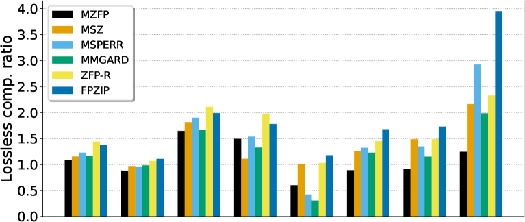
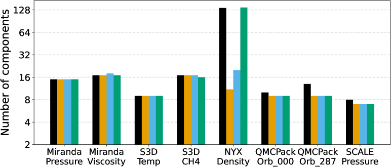
Figure 5: Lossless compression ratio (top) and number of components required by the multi-component compressors (bottom).

4.1.3 Lossless Compression

As alluded to, since each additional component’s inclusion reduces error and since precision is finite, we can achieve fully lossless compression using a sufficient number of components. This allows using lossy compressors without additional redesign for use cases that demand bit-for-bit exact reproducibility.

How competitive is such an approach in terms of compression ratio? Figure 5 plots lossless compression ratios for several fields. For calibration, we also include here results for compressors designed to be lossless: zfp-r (the “reversible” mode of zfp) and fpzip. While our multi-component compressors sacrifice some compression, they still give reasonable compression ratios and often fare not much worse than the specialized methods. Note that idx2 and pmgard do not allow for such lossless compression.

We highlight one challenge that msperr and mmgard have with lossless compression of data containing zeros. Because these compressors perform floating-point arithmetic involving basis functions with wide support, many zero-values are often initially approximated as slightly nonzero. With each subsequent component, those nonzeros are brought closer to zero, but getting all the way to zero requires going through tolerances spanning the subnormal range, with associated components that each have a nonnegligible coding cost. This phenomenon is illustrated in Fig. 6.

4.2 Performance Analysis

We now investigate the serial execution time of Algorithms 1 and 2 for constructing the multi-component representation and later reconstructing a field, respectively. Since the overall trends of the four multi-component approaches are consistent across different data sets, we focus only on the results for the Miranda pressure field. We refer the reader to the supplemental material for other fields. For the multi-component and progressive compressors, the timings reported are cumulative with respect to the number of components, while in the case of the single-component compressors, we report the time to (de)compress the whole data set (as a single component).

4.2.1 Multi-Component Construction and Reconstruction

Figure 7 plots construction (top) and reconstruction (bottom) time, i.e., execution time for Algorithms 1 and 2, for the multi-component compressors based on three granularities as a function of the smallest error tolerance $\tau_{n}$ requested by the user. For comparison purposes, we include the execution time of each corresponding single-component compressor and its projected time, denoted proj, when executed as many times as iterations made by the corresponding multi-component compressors. Analyzing first the top four plots, we note that, except for mgard, all multi-component compressors show execution times in the interval between the single-component compressor and projected times. In addition, the gap between single- and multi-component compressor time decreases with coarser granularity, $\Delta$. This happens because, for a given error tolerance, fewer components are generated with larger $\Delta$, thus the number of calls to the most time consuming steps in Algorithm 1 (Lines $4$ and $5$) is also smaller. Looking at the slope of the curves, we note that mzfp, msz, and msperr start with small inclinations, transition to larger ones as new components get added, and tend to finish with a flat profile when approaching lossless compression. This behavior is related to the inverted U-shape of the component rates shown in Fig. 4, since compression time tends to be proportional to compressed size. Note that in practice, one would set a single finest error tolerance during construction instead of repeating compression runs with different tolerances, as done for these plots.

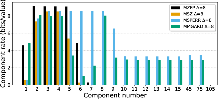
Figure 6: msperr and mmgard sometimes require many components to achieve lossless compression for data containing zeros (here the Nyx dark matter density field).

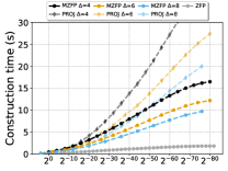
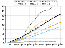
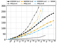
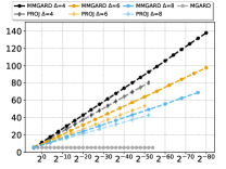
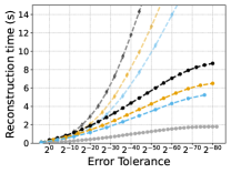
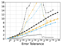
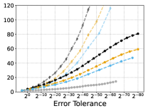
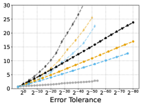
Figure 7: Construction time (top) and reconstruction time (bottom) vs. error tolerance for our multi-component approach based on (from left to right) zfp, sz, sperr, and mgard. The multi-component approaches exhibit longer execution times than their single-component counterparts, though generally less time than linearly scaling the single-component time by the corresponding number of components (labeled proj).

Moving our discussion to reconstruction time, we note that mzfp, msz and msperr behave very similarly to the case of construction, and the same conclusions drawn above apply here. The main difference between construction and reconstruction time is that, for a given error tolerance or number of components, the latter is always smaller for any granularity of the multi-component approach. This is expected since the main cost of Algorithm 2 is running the decompressor, a task also included in Algorithm 1. Lastly, we note that mmgard shows behavior different from before. In fact, the decompression algorithm of mgard depends on the amount of data decoded, and since this varies with the number of components, as shown in Fig. 4, the reconstruction time for mmgard becomes bounded by the projected worst-case time.

4.2.2 Comparison with Progressive Compressors

Lastly, in Fig. 8, we evaluate how the performance of the multi-component techniques compares against idx2 and pmgard. For this purpose, we select the results for $\Delta=8$. We note that idx2 does not support an absolute error tolerance; rather, it is driven by a user-specified target $L_{2}$ error. To allow a fair comparison, we therefore plot (de)compression time as a function of measured maximum absolute ($L_{\infty}$) error, which strongly correlates with error tolerance for the other compressors.

Looking first at compression times, we note that the progressive compressors show a considerable overhead starting from the loosest error tolerance. This is associated with the additional metadata required by them to achieve progressivity. Next, we observe that the multi-component compressors msperr and mmgard are less efficient than the progressive compressors mainly, and this is due to the higher costs of running their underlying compressors (sperr and mgard, respectively). On the other hand, mzfp and msz benefit from their faster underlying compressors. As a result, these techniques are similar in performance to idx2 and pmgard.

Finally, moving to data reconstruction times, all multi-component techniques but msperr are faster than idx2, while mmgard and pmgard give similar performance. From these results, we can affirm that our multi-component approach is competitive in performance with other progressive compressors available in the literature.

4.3 Progressive Use Case

We conclude this section with an example use case of progressive compression that highlights varying precision requirements for different visualization tasks involving derivatives. Spatial derivatives are central to numerous scientific visualization and data analysis techniques, including gradients for volume rendering [11], curl for vortex detection [21], and second derivatives for extraction of ridges and Lagrangian coherent structures [46]. As is well known [44, §5.1.2], differential operators magnify round-off and, by extension, compression errors—the round-off error in the $i^{\text{th}}$ derivative follows $O(h^{-i})$, where $h$ is the grid spacing. Thus, as $h$ approaches zero, derivative estimates are increasingly susceptible to compression artifacts.

In Fig. 9, we visualize the third component of the Miranda velocity field, $\mathbf{u}=(u,v,w)$, which at even a relatively high tolerance $\tau_{1}=1$ yields a quite acceptable result (top left panel). The middle column shows the third component $v_{x}-u_{y}$ of the vorticity field, $\nabla\times\mathbf{u}$, computed from the progressive reconstruction, which at the largest tolerance exhibits significant artifacts. This is because the finite-difference operator used to compute the curl greatly magnifies the compression errors in $\mathbf{u}$. At a tighter tolerance $\tau_{2}=2^{-4}$, however, the vorticity is relatively artifact free (second row). The rightmost column shows the second spatial derivative, $w_{zz}$, a quantity related to viscosity in viscous flows. Clearly $\tau_{1}$ is insufficient, and even $\tau_{2}$ results in major artifacts. The higher sensitivity of the second derivative operator requires an even finer tolerance, $\tau_{3}=2^{-9}$, for acceptable results (bottom row). These varying degrees of sensitivity of data analysis and visualization tasks to compression errors is why it is difficult to a priori choose a single error tolerance and why progressive compression is an attractive solution.

For additional examples of progressive visualizations and quantitative results, we direct the reader to the extensive supplemental material accompanying this paper.

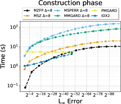
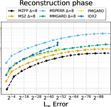
Figure 8: Construction (left) and reconstruction (right) time vs. error tolerance for the multi-component and progressive compressors. Performance wise, our multi-component methods, especially mzfp and msz, are competitive with if not superior to idx2 and pmgard.

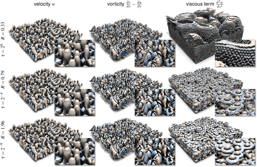
Figure 9: Magnification of mzfp compression errors by differential operators of increasing order (left to right), requiring progressively smaller error tolerances, $\tau$, and correspondingly higher cumulative bit rates, $R$, via additional components (top to bottom).

5 Discussion and Conclusion

We have developed a framework for progressive-precision compression and reconstruction of floating-point scalar fields based on the notion of a multi-component expansion, in which independently-compressed components are successively added to form an ever more faithful approximation. Extensive experiments with real data show that our approach yields competitive rate-distortion tradeoff and performance with two state-of-the-art progressive compressors, while being far prior work, we support fully lossy to lossless compression while requiring no specializations to ensure losslessness. As presented, our framework supports a sequence of absolute error bounds specified by the user at any desired granularity.

5.1 Limitations

We would like to acknowledge some limitations of our approach. First, storage of multiple components may introduce per-component overhead paid only once in conventional single-component compression, and which would likely be absent if one painstakingly re-engineered an otherwise capable single-component compressor to support progressive access, like the two compressors we compare with. The per-component overhead is felt also in compression and decompression time, though our framework achieves competitive and even superior performance over state of the art. Any such overhead is best hidden using fewer components, which unfortunately implies less fine-grained access. We do note, however, that GPU implementations of zfp [38], sz [49], and mgard [8], which could easily be used within our framework, achieve throughputs that are two to three orders of magnitude higher than per-node I/O bandwidth to high-end parallel file systems, effectively eliminating the performance cost of having to compress multiple components.

Contrary to representations designed for in-memory compressed storage [37, 45, 16, 34, 23], our framework, like other progressive compression techniques [25, 26, 29, 32, 6], incrementally refines an uncompressed representation, $\tilde{\mathbf{x}}$. Enough CPU or GPU memory for this reconstruction as well as a temporary buffer for one decompressed component, $\mathbf{x}_{i}$, is assumed. The space for this temporary buffer can be significantly reduced using data chunking techniques, as employed for example in tthresh [4], sperr [30], and—to a more extreme degree—zfp, where single $d$-dimensional blocks of $4^{d}$ scalars can be decompressed at a time and added into $\tilde{\mathbf{x}}$.

We may also reduce the in-memory storage cost for $\tilde{\mathbf{x}}$. Though specific to mzfp, we may keep the components $\{\mathbf{y}_{i}\}$ in compressed form and decompress and add blocks on demand to form requested pieces of $\tilde{\mathbf{x}}$. As we have seen, the overhead of multiple compressed components over a single compressed sum of components is often marginal. We also suggest a more general hybrid approach that maintains $\tilde{\mathbf{x}}$ not in double-precision floating point but as a zfp array. Toward this end, zfp 1.0.0 supports both fixed-rate and error-bounded variable-rate arrays, allowing significant storage to be saved while retaining fast random access and sequential updates. As we are unaware of any solution that currently supports progressive updates of in-memory compressed arrays, we view such an approach as an exciting new research opportunity.

While we are not married to any particular error metric or parameters that drive the compression process, supporting pointwise relative error bounds may be challenging. One could, however, evaluate relative errors a posteriori and store such per-component errors as metadata. Finally, our support for lossless compression is limited to numerical data—NaNs, infinities, and signed zeros are not handled.

5.2 Benefits

Our approach also has several distinct benefits. For one, it is compressor agnostic and can hence trivially be made to work with any lossy compressor (and compressor parameters) or novel number representation, like posits [22]. In fact, one may even employ different compressors for different components, e.g., by using computationally expensive but effective compressors only for the first few components. As we have seen, decomposing the data into multiple components can in fact boost compression (as in the case of sz) or accuracy (as in the case of zfp and mgard). No custom progressive file format is needed; indeed, our approach integrates directly into popular I/O formats/libraries like HDF5 and ADIOS, with the sole change being how consumers interpret the additional “component dimension.” To meet any requested error tolerance, the prescribed tolerances or measured errors would be stored as per-component metadata that the user can consult to request a sufficient number of components. To progressively increase precision, one simply decompresses additional components and adds them to the current approximation, with no need to maintain decompressor state.

One potential benefit of the complete decoupling of components is that they need not be stored together. As suggested in [32], one may utilize slower media like tape for the least significant, rarely accessed components. One may take this one step further and distribute and cache compressed components throughout the memory hierarchy, from CPU and GPU RAM to node-local storage, parallel spinning disk, tape archives, and even remote compute facilities and databases. The distinct separation of components makes this approach conceptually simple.

Finally, we acknowledge that our approach is embarrassingly straightforward. However, we view its simplicity and effectiveness features that make for a very intuitive and pragmatic solution to incorporating progressive compression and access into existing pipelines in a rather nondisruptive fashion. We envision that many community databases could incorporate our framework by simply adding an extra “component dimension” to data variables using some agreed upon naming convention. We see such application integrations as important avenues for future work.

- [1] M. Ainsworth, O. Tugluk, B. Whitney, and S. Klasky. Multilevel techniques for compression and reduction of scientific data—the multivariate case. SIAM Journal on Scientific Computing, 41(2):A1278––A1303, 2019. doi: 10 . 1137/18M1166651
- [2] I. Antcheva, M. Ballintijn, B. Bellenot, M. Biskup, R. Brun, N. Buncic, P. Canal, D. Casadei, O. Couet, V. Fine, L. Franco, G. Ganis, A. Gheata, D. G. Maline, M. Goto, J. Iwaszkiewicz, A. Kreshuk, D. M. Segura, R. Maunder, L. Moneta, A. Naumann, E. Offermann, V. Onuchin, S. Panacek, F. Rademakers, P. Russo, and M. Tadel. ROOT – a C++ framework for petabyte data storage, statistical analysis and visualization. Computer Physics Communications, 180(12):2499–2512, 2009. doi: 10 . 1016/j . cpc . 2009 . 08 . 005
- [3] G. Ballard, A. Klinvex, and T. G. Kolda. TuckerMPI: A parallel C++/MPI software package for large-scale data compression via the Tucker tensor decomposition. ACM Transactions on Mathematical Software, 46(2):13:1–31, 2020. doi: 10 . 1145/3378445
- [4] R. Ballester-Ripoll, P. Lindstrom, and R. Pajarola. TTHRESH: Tensor compression for multidimensional visual data. IEEE Transactions on Visualization and Computer Graphics, 26(9):2891–2903, 2020. doi: 10 . 1109/TVCG . 2019 . 2904063
- [5] B. Barbarioli, G. Mersy, S. Sintos, and S. Krishnan. Hierarchical residual encoding for multiresolution time series compression. Proceedings of the ACM on Management of Data, 1(1):99:1–26, 2023. doi: 10 . 1145/3588953
- [6] H. Bhatia, D. Hoang, N. Morrical, V. Pascucci, P.-T. Bremer, and P. Lindstrom. AMM: Adaptive multilinear meshes. IEEE Transactions on Visualization and Computer Graphics, 28(6):2350–2363, 2022. doi: 10 . 1109/TVCG . 2022 . 3165392
- [7] P. J. Burt and E. H. Adelson. The Laplacian Pyramid as a compact image code. In M. A. Fischler and O. Firschein, eds., Readings in Computer Vision, pp. 671–679. Morgan Kaufmann, 1987. doi: 10 . 1016/B978-0-08-051581-6 . 50065-9
- [8] J. Chen, L. Wan, X. Liang, B. Whitney, Q. Liu, D. Pugmire, N. Thompson, J. Y. Choi, M. Wolf, T. Munson, I. Foster, and S. Klasky. Accelerating multigrid-based hierarchical scientific data refactoring on GPUs. In IEEE International Parallel and Distributed Processing Symposium, pp. 859–868, 2021. doi: 10 . 1109/IPDPS49936 . 2021 . 00095
- [9] C. Christopoulos, A. Skodras, and T. Ebrahimi. The JPEG2000 still image coding system: An overview. IEEE Transactions on Consumer Electronics, 46(4):1103–1127, 2000. doi: 10 . 1109/30 . 920468
- [10] J. Clyne. Progressive data access for regular grids. In E. W. Bethel, H. Childs, and C. Hansen, eds., High Performance Visualization, pp. 145–169. Chapman and Hall/CRC, 2012. doi: 10 . 1201/b12985-19
- [11] C. D. Correa, R. Hero, and K.-L. Ma. A comparison of gradient estimation methods for volume rendering on unstructured meshes. IEEE Transactions on Visualization and Computer Graphics, 17(3):305–319, 2011. doi: 10 . 1109/TVCG . 2009 . 105
- [12] T. J. Dekker. A floating-point technique for extending the available precision. Numerische Mathematik, 18:224–242, 1971. doi: 10 . 1007/BF01397083
- [13] J. Diffenderfer, A. L. Fox, J. A. Hittinger, G. Sanders, and P. G. Lindstrom. Error analysis of ZFP compression for floating-point data. SIAM Journal on Scientific Computing, 41(3):A1867–A1898, 2019. doi: 10 . 1137/18M1168832
- [14] V. Eyring, S. Bony, G. A. Meehl, C. A. Senior, B. Stevens, R. J. Stouffer, and K. E. Taylor. Overview of the coupled model intercomparison project phase 6 (CMIP6) experimental design and organization. Geoscientific Model Development, 9(5):1937–1958, 2016. doi: 10 . 5194/gmd-9-1937-2016
- [15] M. Folk, G. Heber, Q. Koziol, E. Pourmal, and D. Robinson. An overview of the HDF5 technology suite and its applications. In EDBT/ICDT 2011 Workshop on Array Databases, pp. 36–47, 2011. doi: 10 . 1145/1966895 . 1966900
- [16] N. Fout and K.-L. Ma. Transform coding for hardware-accelerated volume rendering. IEEE Transactions on Visualization and Computer Graphics, 13(6):1600–1607, 2007. doi: 10 . 1109/TVCG . 2007 . 70516
- [17] W. F. Godoy, N. Podhorszki, R. Wang, C. Atkins, G. Eisenhauer, J. Gu, P. Davis, J. Choi, K. Germaschewski, K. Huck, A. Huebl, M. Kim, J. Kress, T. Kurc, Q. Liu, J. Logan, K. Mehta, G. Ostrouchov, M. Parashar, F. Poeschel, D. Pugmire, E. Suchyta, K. Takahashi, N. Thompson, S. Tsutsumi, L. Wan, M. Wolf, K. Wu, and S. Klasky. ADIOS 2: The adaptable input output system. A framework for high-performance data management. SoftwareX, 12:1–9, 2020. doi: 10 . 1016/j . softx . 2020 . 100561
- [18] Q. Gong, B. Whitney, C. Zhang, X. Liang, A. Rangarajan, J. Chen, L. Wan, P. Ullrich, Q. Liu, R. Jacob, S. Ranka, and S. Klasky. Region-adaptive, error-controlled scientific data compression using multilevel decomposition. In International Conference on Scientific and Statistical Database Management, pp. 5:1–5:12, 2022. doi: 10 . 1145/3538712 . 3538717
- [19] J. Graham, K. Kanov, X. I. A. Yang, M. Lee, N. Malaya, C. C. Lalescu, R. Burns, G. Eyink, A. Szalay, R. D. Moser, and C. Meneveau. A web services accessible database of turbulent channel flow and its use for testing a new integral wall model for LES. Journal of Turbulence, 17(2):181–215, 2016. doi: 10 . 1080/14685248 . 2015 . 1088656
- [20] R. W. Grout, A. Gruber, H. Kolla, P.-T. Bremer, J. C. Bennett, A. Gyulassy, and J. J. Chen. A direct numerical simulation study of turbulence and flame structure in transverse jets analysed in jet-trajectory based coordinates. Journal of Fluid Mechanics, 706:351–383, 2012. doi: 10 . 1017/jfm . 2012 . 257
- [21] T. Günther and H. Theisel. The state of the art in vortex extraction. Computer Graphics Forum, 37(6):149–173, 2018. doi: 10 . 1111/cgf . 13319
- [22] J. L. Gustafson and I. T. Yonemoto. Beating floating point at its own game: Posit arithmetic. Supercomputing Frontiers and Innovations, 4(2):71–86, 2017. doi: 10 . 14529/jsfi170206
- [23] S. Guthe and M. Goesele. Variable length coding for GPU-based direct volume rendering. In Vision, Modeling & Visualization, pp. 77–84, 2016. doi: 10 . 2312/vmv . 20161345
- [24] Y. Hida, X. S. Li, and D. H. Bailey. Algorithms for quad-double precision floating point arithmetic. In 15th IEEE Symposium on Computer Arithmetic, pp. 155–162, 2001. doi: 10 . 1109/ARITH . 2001 . 930115
- [25] D. Hoang, P. Klacansky, H. Bhatia, P.-T. Bremer, P. Lindstrom, and V. Pascucci. A study of the trade-off between reducing precision and reducing resolution for data analysis and visualization. IEEE Transactions on Visualization and Computer Graphics, 25(1):1193–1203, 2019. doi: 10 . 1109/TVCG . 2018 . 2864853
- [26] D. Hoang, B. Summa, P. Klacansky, W. Usher, H. Bhatia, P. Lindstrom, P.-T. Bremer, and V. Pascucci. Efficient and flexible hierarchical data layouts for a unified encoding of scalar field precision and resolution. IEEE Transactions on Visualization and Computer Graphics, 27(2):603–613, 2021. doi: 10 . 1109/TVCG . 2020 . 3030381
- [27] E. S. Hong, R. E. Ladner, and E. A. Riskin. Group testing for block transform image compression. In Asilomar Conference on Signals, Systems and Computers, pp. 769–772, 2001. doi: 10 . 1109/ACSSC . 2001 . 987028
- [28] J. E. Kay, C. Deser, A. Phillips, A. Mai, C. Hannay, G. Strand, J. Arblaster, S. Bates, G. Danabasoglu, J. Edwards, M. Holland, P. Kushner, J.-F. Lamarque, D. Lawrence, K. Lindsay, A. Middleton, E. Munoz, R. Neale, K. Oleson, L. Polvani, and M. Vertenstein. The community earth system model (CESM) large ensemble project: A community resource for studying climate change in the presence of internal climate variability. Bulletin of the American Meteorological Society, 96:1333–1349, 2015. doi: 10 . 1175/BAMS-D-13-00255 . 1
- [29] S. Li, S. Jaroszynski, S. Pearse, L. Orf, and J. Clyne. VAPOR: A visualization package tailored to analyze simulation data in earth system science. Atmosphere, 10(9):1–22, 2019. doi: 10 . 3390/atmos10090488
- [30] S. Li, P. Lindstrom, and J. Clyne. Lossy scientific data compression with SPERR. In IEEE International Parallel and Distributed Processing Symposium, pp. 1007–1017, 2023. doi: 10 . 1109/IPDPS54959 . 2023 . 00104
- [31] S. Li, N. Marsaglia, C. Garth, J. Woodring, J. Clyne, and H. Childs. Data reduction techniques for simulation, visualization and data analysis. Computer Graphics Forum, 37(6):422–447, 2018. doi: 10 . 1111/cgf . 13336
- [32] X. Liang, Q. Gong, J. Chen, B. Whitney, L. Wan, Q. Liu, D. Pugmire, R. Archibald, N. Podhorszki, and S. Klasky. Error-controlled, progressive, and adaptable retrieval of scientific data with multilevel decomposition. In International Conference for High Performance Computing, Networking, Storage and Analysis, pp. 88:1–88:13, 2021. doi: 10 . 1145/3458817 . 3476179
- [33] X. Liang, K. Zhao, S. Di, S. Li, R. Underwood, A. M. Gok, J. Tian, J. Deng, J. C. Calhoun, D. Tao, Z. Chen, and F. Cappello. SZ3: A modular framework for composing prediction-based error-bounded lossy compressors. IEEE Transactions on Big Data, 9(2):485–498, 2023. doi: 10 . 1109/TBDATA . 2022 . 3201176
- [34] P. Lindstrom. Fixed-rate compressed floating-point arrays. IEEE Transactions on Visualization and Computer Graphics, 20(12):2674–2683, 2014. doi: 10 . 1109/TVCG . 2014 . 2346458
- [35] P. Lindstrom. MultiPosits: Universal coding of . In Conference on Next Generation Arithmetic, pp. 66–83, 2022. doi: 10 . 1007/978-3-031-09779-9_5
- [36] P. Lindstrom and M. Isenburg. Fast and efficient compression of floating-point data. IEEE Transactions on Visualization and Computer Graphics, 12(5):1245–1250, 2006. doi: 10 . 1109/TVCG . 2006 . 143
- [37] P. Ning and L. Hesselink. Vector quantization for volume rendering. In ACM Workshop on Volume Visualization, pp. 69–74, 1992. doi: 10 . 1145/147130 . 147152
- [38] L. Noordsij, S. v. d. Vlugt, M. A. Bamakhrama, Z. Al-Ars, and P. Lindstrom. Parallelization of variable rate decompression through metadata. In Euromicro International Conference on Parallel, Distributed and Network-Based Processing, pp. 245–252, 2020. doi: 10 . 1109/PDP50117 . 2020 . 00045
- [39] V. Pascucci and R. J. Frank. Global static indexing for real-time exploration of very large regular grids. In ACM/IEEE Conference on Supercomputing, pp. 1–8, 2001. doi: 10 . 1145/582034 . 582036
- [40] W. Pearlman, A. Islam, N. Nagaraj, and A. Said. Efficient, low-complexity image coding with a set-partitioning embedded block coder. IEEE Transactions on Circuits and Systems for Video Technology, 14(11):1219–1235, 2004. doi: 10 . 1109/TCSVT . 2004 . 835150
- [41] A. J. Peters and L. Janyst. Exabyte scale storage at CERN. Journal of Physics, 331(5):1–6, 2011. doi: 10 . 1088/1742-6596/331/5/052015
- [42] R. Rew and G. Davis. NetCDF: an interface for scientific data access. IEEE Computer Graphics and Applications, 10(4):76–82, 1990. doi: 10 . 1109/38 . 56302
- [43] A. Said and W. A. Pearlman. A new, fast, and efficient image codec based on set partitioning in hierarchical trees. IEEE Transactions on circuits and systems for video technology, 6(3):243–250, 1996. doi: 10 . 1109/76 . 499834
- [44] T. Sauer. Numerical Analysis. Pearson, 3rd ed., 2018.
- [45] J. Schneider and R. Westermann. Compression domain volume rendering. In IEEE Visualization, pp. 293–300, 2003. doi: 10 . 1109/VISUAL . 2003 . 1250385
- [46] S. C. Shadden, F. Lekien, and J. E. Marsden. Definition and properties of Lagrangian coherent structures from finite-time Lyapunov exponents in two-dimensional aperiodic flows. Physica D: Nonlinear Phenomena, 212(3):271–304, 2005. doi: 10 . 1016/j . physd . 2005 . 10 . 007
- [47] J. M. Shapiro. Embedded image coding using zerotrees of wavelet coefficients. IEEE Transactions on Signal Processing, 41(12):3445–3462, 1993. doi: 10 . 1109/78 . 258085
- [48] J. R. Shewchuk. Adaptive precision floating-point arithmetic and fast robust geometric predicates. Discrete & Computational Geometry, 18(3):305–363, 1997. doi: 10 . 1007/PL00009321
- [49] J. Tian, S. Di, K. Zhao, C. Rivera, M. H. Fulp, R. Underwood, S. Jin, X. Liang, J. Calhoun, D. Tao, and F. Cappello. cuSZ: An efficient GPU-based error-bounded lossy compression framework for scientific data. In ACM International Conference on Parallel Architectures and Compilation Techniques, pp. 3––15, 2020. doi: 10 . 1145/3410463 . 3414624
- [50] Željko Ivezić, S. M. Kahn, J. A. Tyson, B. Abel, E. Acosta, R. Allsman, D. Alonso, Y. AlSayyad, S. F. Anderson, and J. Andrew. LSST: From science drivers to reference design and anticipated data products. The Astrophysical Journal, 873(2):1–44, 2019. doi: 10 . 3847/1538-4357/ab042c
- [51] J. H. Wilkinson. Rounding Errors in Algebraic Processes. Prentice Hall, 1963. doi: 10 . 1137/1 . 9781611977523
- [52] J. Zhang, X. Zhuo, A. Moon, H. Liu, and S. W. Son. Efficient encoding and reconstruction of HPC datasets for checkpoint/restart. In Symposium on Mass Storage Systems and Technologies, pp. 79–91, 2019. doi: 10 . 1109/MSST . 2019 . 00-14
- [53] K. Zhao, S. Di, X. Lian, S. Li, D. Tao, J. Bessac, Z. Chen, and F. Cappello. SDRBench: Scientific data reduction benchmark for lossy compressors. In IEEE International Conference on Big Data, pp. 2716–2724, 2020. https://sdrbench.github.io. doi: 10 . 1109/BigData50022 . 2020 . 9378449