Model-free Learning with Heterogeneous Dynamical Systems: A Federated LQR Approach

Abstract

We study a model-free federated linear quadratic regulator (LQR) problem where $M$ agents with unknown, distinct yet similar dynamics collaboratively learn an optimal policy to minimize an average quadratic cost while keeping their data private. To exploit the similarity of the agents’ dynamics, we propose to use federated learning (FL) to allow the agents to periodically communicate with a central server to train policies by leveraging a larger dataset from all the agents. With this setup, we seek to understand the following questions: (i) Is the learned common policy stabilizing for all agents? (ii) How close is the learned common policy to each agent’s own optimal policy? (iii) Can each agent learn its own optimal policy faster by leveraging data from all agents? To answer these questions, we propose a federated and model-free algorithm named FedLQR. Our analysis overcomes numerous technical challenges, such as heterogeneity in the agents’ dynamics, multiple local updates, and stability concerns. We show that FedLQR produces a common policy that, at each iteration, is stabilizing for all agents. We provide bounds on the distance between the common policy and each agent’s local optimal policy. Furthermore, we prove that when learning each agent’s optimal policy, FedLQR achieves a sample complexity reduction proportional to the number of agents $M$ in a low-heterogeneity regime, compared to the single-agent setting.

1 Introduction

In recent years, there has been significant progress in the application of model-free reinforcement learning (RL) methods to fields such as video games (Mnih et al., 2015) and robotic manipulation (Rajeswaran et al., 2017; Levine et al., 2016; Tobin et al., 2017). Although RL has shown impressive results in simulation, it often suffers from poor sample complexity, thereby limiting its effectiveness in real-world applications (Dulac-Arnold et al., 2019). To resolve the sample complexity issue and accelerate the learning process, federated learning (FL) has emerged as a popular paradigm  (Konečnỳ et al., 2016a; McMahan et al., 2017), where multiple similar agents collaboratively learn a common model without sharing their raw data. The incentive for collaboration arises from the fact that these agents are “similar” in some sense and hence end up learning a “superior” model than if they were to learn alone. In the RL setting, Federated Reinforcement Learning (FRL) aims to learn a common value function (Wang et al., 2023) or produce a better policy from multiple RL agents interacting with similar environments. In the recent survey paper (Qi et al., 2021), FRL has empirically shown great success in reducing the sample complexity in applications such as autonomous driving (Liang et al., 2022), IoT devices (Lim et al., 2020), and resource management in networking (Yu et al., 2020).

Lately, there has been a lot of interest in applying RL techniques to classical control problems such as the Linear Quadratic Regulaor (LQR) problem (Anderson and Moore, 2007). In the standard control setting, the dynamical model of the system is known and one seeks to obtain a controller that stabilizes the closed-loop system and provides optimal performance. RL approaches such as policy gradient (Williams, 1992; Sutton et al., 1999) (which we pursue here) differ in that they are “model-free”, i.e., a control policy is obtained despite not having access to the model of the dynamics. Despite the lack of convexity in even simple problems, policy gradient (PG) methods have been shown to be globally convergent for certain structured settings such as the LQR problem (Fazel et al., 2018). While this is promising, a major challenge in applying PG methods is that in general, one does not have access to exact deterministic policy gradients. Instead, one relies on estimating such gradients via sampling based approaches. This typically leads to noisy gradients that can suffer from high variance. As such, reducing the variance in PG estimates to achieve “good performance" may end up requiring several samples.

Motivation. The main premise of this paper is to draw on ideas from the FL literature to alleviate the high sample-complexity burden of PG methods (Agarwal et al., 2019; Wang et al., 2019; Liu et al., 2020), with the focus being on model-free control. As a motivating example, consider a fleet of identical robots produced by the same manufacturer. Each robot can collect data from its own dynamics and learn its own optimal policy using, for instance, PG methods. Since the fleet of robots shares similar dynamics, and more data can potentially lead to improved policy performance (via more accurate PG estimates), it is natural to ask: Can a robot accelerate the process of learning its own optimal policy by leveraging the data of the other robots in the fleet? The answer is not as obvious as one might expect since in reality, it is unlikely that any two robots will have exactly the same underlying dynamics, i.e., heterogeneity in system dynamics is inevitable. The presence of such heterogeneity makes the question posed above both interesting and non-trivial. In particular, when the heterogeneity across agents’ dynamics is large, leveraging data from other agents might degrade the performance of a single agent. Indeed, large heterogeneity may make it impossible to learn a common stabilizing policy. Moreover, even when such a stabilizing policy exists, it may deviate from each agent’s local optimal policy, rendering poor performance and discouraging participation in the FL process. Thus, to understand whether more data helps or hurts, it is crucial to characterize the effects of heterogeneity in the federated control setting.

With this aim in mind, we study a multi-agent model-free LQR problem based on policy gradient methods. Specifically, there are $M$ agents in our setup, each with its own distinct yet similar linear time-invariant (LTI) dynamics. Inspired by the typical objective in FL, our goal is to find a common policy which can minimize the average of the LQR costs of all the agents. With this setup, we seek to answer the following questions.

Q1. Is this common policy stabilizing for all the systems? If so, under what conditions?

Q2. How far is the learned common policy from each agent’s locally optimal policy?

Q3. Can an agent use the common policy as an initial guess to fine-tune and learn its own optimal policy faster (i.e., with fewer overall samples) than if it acted alone?

Challenges: There are several challenges to answering the above questions. First, even for the single agent setting, the policy gradient-based LQR problem is non-convex, and requires a fairly intricate analysis (Fazel et al., 2018). Second, a key distinction relative to standard federated supervised learning stems from the need to maintain stability – this problem is amplified in the heterogeneous multi-agent scenario we consider. It remains an open problem to design an algorithm ensuring that policies are simultaneously stabilizing for each distinct system. Third, to reduce the communication cost, FL algorithms rely on the agents performing multiple local update steps between successive communication rounds. When agents have non-identical loss functions, these local steps lead to a “client-drift" effect where each agent drifts towards its own local minimizer (Charles and Konečnỳ, 2020a, 2021a). While several works in FL have investigated this phenomenon (Li et al., 2020; Khaled et al., 2019a, 2020; Li et al., 2019a; Karimireddy et al., 2020; Pathak and Wainwright, 2020a; Wang et al., 2020a; Acar et al., 2021; Gorbunov et al., 2021; Mitra et al., 2021; Mishchenko et al., 2022; Laguel et al., 2021), the effect of “client-drift" on stability remains completely unexplored. Unless accounted for, such drift effects can potentially produce unstable controllers for some systems.

Our Contributions: In response to the above challenges, we propose a policy gradient method called FedLQR to solve the (model-based and model-free) federated LQR problem, and provide a rigorous finite-time analysis of its performance that accounts for the interplay between system heterogeneity, multiple local steps, client-drift effects, and stability. Our specific contributions in this regard are as follows.

$\bullet$ Iterative stability guarantees. We show via a careful inductive argument that under suitable requirements on the level of heterogeneity across systems, the learning rate schedule can be designed to ensure that FedLQR provides a stabilizing controller at every iteration for all systems. Theorem 3 provides a proof in the model-based setting, and Theorem 5 provides the model-free result.

$\bullet$ Bounded policy gradient heterogeneity in the LQR problem. We prove in Lemma 3 that, for each pair of agents $i,j\in[M],$ the policy gradient direction (in the model-based setting) of agent $i$ is close to that of agent $j$, if their dynamics are similar (i.e., Definition 1). This is the first result to observe and characterize this bounded gradient heterogeneity phenomenon in the multi-agent LQR setting.

$\bullet$ Quantifying the gap between the FedLQR output and locally optimal policies. Building on Lemma 3, we prove that when the agents’ dynamics are similar, the common policy returned by FedLQR is close to each agent’s optimal policy; see Theorem 4. In other words, we can leverage the federated formulation to help each agent find its own optimal policy up to some accuracy depending on the level of heterogeneity. Our work is the first to provide a result of this flavor.

$\bullet$ Linear speedup. As our main contribution, we prove that in the model-free setting, FedLQR converges to a solution that is in a neighborhood of each agent’s optimal policy, using $M$-times fewer samples relative to when each agent just uses its own data (see Theorem 5). The radius of this neighborhood captures the level of heterogeneity across the agents’ dynamics. The key implication of this result is that in a low-heterogeneity regime, FedLQR (in the model-free setting) reduces the sample-complexity by a factor of $M$ w.r.t. the centralized setting (Fazel et al., 2018; Malik et al., 2019), highlighting the benefit of collaboration. Simply put, FedLQR enables each agent to quickly find an approximate locally optimal policy; as in standard FL (Collins et al., 2022), the agent can then use this policy as an initial guess to fine-tune based on its own data.

In summary, we provide a new theoretical framework that quantitatively characterizes the interplay between the price of heterogeneity and the benefit of collaboration for model-free control.

Related Work: There has been a line of work (Fazel et al., 2018; Malik et al., 2019; Hambly et al., 2021; Mohammadi et al., 2021; Gravell et al., 2020; Jin et al., 2020; Ju et al., 2022) that explores various RL algorithms for solving the model-free LQR problem. However, their analysis is limited to the single-agent setting. Most recently, Ren et al. (2020) solves the model-free LQR tracking problem in a federated manner and achieves a linear convergence speedup with respect to the number of agents. However, they consider a simplified setting where all agents follow the same dynamics. As such, the stability analysis of Ren et al. (2020) follows from arguments for the centralized setting. In sharp contrast, to establish the linear speedup for FedLQR, we need to address the key technical challenges arising from the effect of heterogeneity and local steps on the stability of distinct systems. This requires new analysis tools that we develop. For related work on multi-agent RL (that do not specifically look at the control setting) we point the reader to (Lin et al., 2021; Zhang et al., 2021) and the references therein. A more detailed description of related work is given in the Appendix.

2 Problem Setup

Notation: Given a set of matrices $\{S^{(i)}\}_{i=1}^{M}$, we denote $||S||_{\max}:=\max_{i}||S^{(i)}||$, and $||S||_{\min}:=\min_{i}||S^{(i)}||$. All vector norms are Euclidean and matrix norms are spectral, unless otherwise stated.

Classical control approaches aim to design optimal controllers from a well-defined dynamical system model. The model-based LQR is a well-studied problem that admits a convex solution. In this work, we consider the LQR problem but in the model-free setting. Moreover, we consider a federated model-free LQR problem in which there are $M$ agents, each with their own distinct but “similar’ dynamics. Our goal is to collaboratively learn an optimal controller that minimizes an average quadratic cost. We seek to characterize the optimality of our solution as a function of the “difference” across the agent’s dynamics. In what follows, we formally describe our problem of interest.

Federated LQR: Consider a system with $M$ agents. Associated with each agent is a linear time-invariant (LTI) dynamical system of the form

$$x^{(i)}_{t+1}=A^{(i)}x^{(i)}_{t}+B^{(i)}u^{(i)}_{t},\quad x_{0}^{(i)}\sim\mathcal{D},\quad i=1,\ldots,M,$$

with $A^{(i)}\in\mathbb{R}^{n_{x}\times n_{x}}$, $B^{(i)}\in\mathbb{R}^{n_{x}\times n_{u}}$. We assume each initial state $x_{0}^{(i)}$ is randomly generated from the same distribution $\mathcal{D}$. In the single-agent setting, the optimal LQR policy $u_{t}^{(i)}={-}K_{i}^{*}x_{t}^{(i)}$ for each agent is given by the solution to

$$K_{i}^{*}=\arg\min_{K} \left\{C^{(i)}(K):=\mathbb{E}\left[\sum_{t=0}^{\infty}x_{t}^{(i)\top}Qx_{t}^{(i)}+u_{t}^{(i)\top}Ru_{t}^{(i)}\right]\right\}$$

s.t. $$\quad x_{t+1}^{(i)}=A^{(i)}x_{t}^{(i)}+B^{(i)}u_{t}^{(i)},\ u_{t}^{(i)}=-Kx_{t}^{(i)},\ x_{0}^{(i)}\sim\mathcal{D},$$ (1)

where $Q\in\mathbb{R}^{n_{x}\times n_{x}}$ and $R\in\mathbb{R}^{n_{u}\times n_{u}}$ are known positive definite matrices. In our federated setting, the objective is to find an optimal common policy $\{u_{t}\}_{t=0}^{\infty}$ to minimize the average cost of all the agents $C_{\text{avg}}:=\frac{1}{M}\sum_{i=1}^{M}C^{(i)}(K)$ without knowledge of the system dynamics, i.e., ($A^{(i)},B^{(i)}$). Classical results (Anderson and Moore, 2007) from optimal control theory show that, given the system matrices $A^{(i)}$, $B^{(i)}$, $Q$ and $R$, the optimal policy can be written as a linear function of the current state. Thus, we consider a common policy of the form $u_{t}^{(i)}=-Kx_{t}^{(i)}$. The objective of the federated LQR problem can be written as:

$$K^{*}= \arg\min_{K}\left\{C_{\text{avg}}(K):=\frac{1}{M}\sum_{i=1}^{M}\mathbb{E}\left[\sum_{t=0}^{\infty}x_{t}^{(i)\top}Qx_{t}^{(i)}+u_{t}^{(i)\top}Ru_{t}^{(i)}\right]\right\}$$

s.t. $$\quad x_{t+1}^{(i)}=A^{(i)}x_{t}^{(i)}+B^{(i)}u_{t}^{(i)},\quad u^{(i)}_{t}=-Kx_{t}^{(i)},x_{0}^{(i)}\sim\mathcal{D}.$$ (2)

The rationale for finding $K^{*}$ is as follows. Intuitively, when all agents have similar dynamics, $K^{*}$ will be close to each $K_{i}^{*}$. Thus, $K^{*}$ will serve to provide a good common initial guess from which each agent $i$ can then fine-tune/personalize (using only its own data) to converge exactly to its own locally optimal controller $K_{i}^{*}$ . The key here is that the initial guess $K^{*}$ can be obtained quickly by using the collective data of all the agents. We will formalize this intuition in Theorem 5.

We make the standard assumption that for each agent, $(A^{(i)},B^{(i)})$ is stabilizable. In addition, we make the following assumption on the distribution of the initial state:

Assumption 1.

Let $\mu:=\sigma_{\min}\left(\mathbb{E}_{x^{(i)}_{0}\sim\mathcal{D}}x^{(i)}_{0}x^{(i)\top}_{0}\right)$ and assume $\mu>0.$ For each $i\in[M],$ the initial state $x_{0}^{(i)}\sim\mathcal{D}$ and distribution $\mathcal{D}$ satisfy

$$\mathbb{E}_{x_{0}^{(i)}\sim\mathcal{D}}[x_{0}^{(i)}]=0,\quad\mathbb{E}_{x_{0}^{(i)}\sim\mathcal{D}}[x_{0}^{(i)}x_{0}^{(i)\top}]\succ\mu\mathbb{I}_{d_{x}},\quad\text{and}\quad\lVert x_{0}^{(i)}\rVert\leq H\\ \ \text{ almost surely. }$$

We quantify the heterogeneity in the agent’s dynamics through the following definition:

Definition 1.

(Bounded system heterogeneity) There exist positive constants $\epsilon_{1}$ and $\epsilon_{2}$ such that

$$\underset{i,j\in[M]}{\max}\lVert A^{(i)}-A^{(j)}\rVert\leq\epsilon_{1},\text{ and }\underset{i,j\in[M]}{\max}\lVert B^{(i)}-B^{(j)}\rVert\leq\epsilon_{2}.$$

We assume that $\epsilon_{1}$ and $\epsilon_{2}$ are finite. Similar bounded heterogeneity assumptions are commonly made in FL (Karimireddy et al., 2020; Khaled et al., 2020; Reddi et al., 2020). However, unlike typical FL works where one directly imposes heterogeneity assumptions on the agents gradients, in our setting, we need to carefully characterize how heterogeneity in the system parameters $(A^{(i)},B^{(i)})$ translates to differences in the policy gradients; see Lemma 3.

Before providing our solution to the federated LQR problem, we first recap existing results on model-free LQR in the single-agent setting.

The single-agent setting: When there is only one agent, i.e., $M=1$, let us denote the system matrix as $(A,B)$. If $(A,B)$ is known, the optimal controller $K^{*}$ can be computed by solving the discrete-time Algebraic Riccati Equation (ARE) (Anderson and Moore, 2007).

Strikingly, (Fazel et al., 2018) show that policy gradient methods can find the globally optimal LQR policy $K^{*}$ despite the non-convexity of the problem. Tthe policy gradient of the LQR problem can be expressed as:

$$\nabla C(K)=2E_{K}\Sigma_{K}=2\left(\left(R+B^{\top}P_{K}B\right)K-B^{\top}P_{K}A\right)\Sigma_{K},$$

where $P_{K}$ is the positive definite solution to the Lyapunov equation: $P_{K}=Q+K^{\top}RK+(A-BK)^{\top}P_{K}(A-BK),$ $E_{K}:=\left(R+B^{\top}P_{K}B\right)K-B^{\top}P_{K}A$, and $\Sigma_{K}:=\mathbb{E}_{x_{0}\sim\mathcal{D}}\sum_{t=0}^{\infty}x_{t}x_{t}^{\top}.$ The policy gradient method $K\leftarrow K-\eta\nabla C(K)$ will find the global optimal LQR policy, i.e., $K\rightarrow K^{*}$, provided that $\mathbb{E}_{x_{0}\sim\mathcal{D}}[x_{0}x_{0}^{\top}]$ is full rank and an initial stabilizing policy is used. When the model is unknown, the analysis technique employed by Fazel et al. (2018) is to construct near-exact gradient estimates from reward samples and show that the sample complexity of such a method is bounded polynomially in the parameters of the problem.

In contrast to the single-agent setting, the heterogeneous, multi-agent scenario we consider here is considerably more difficult to analyze. First, designing an algorithm satisfying the iterative stability guarantees becomes a complex task. Second, since each agent in the system has its own unique dynamics and gradient estimates, it can be difficult to aggregate these directions in a manner that ensures the updating direction moves toward the average optimal policy $K^{*}$. Nonetheless, in the sequel, we will overcome these challenges and provide a finite-time analysis of FedLQR.

3 Necessity of the Low Heterogeneity Requirement

In our main theorems, we require certain bounds on the parameters $\epsilon_{1}$ and $\epsilon_{2}$ that define the heterogeneity of the $M$ dynamical systems we work with. Here, we point out that, unlike standard federated learning settings, these bounds are necessary for convergence. From a control and dynamical systems viewpoint, these bounds are perhaps intuitive: if the systems are too different, then there is no reason to believe there exists a stabilizing controller, i.e., there is no solution to the problem (2). In what follows, we will formalize this point. To do so, let us define an “instance" of our FedLQR problem via a parameter $M$ that characterizes the number of agents/systems and the set of corresponding system matrices $\{A^{(i)},B^{(i)}\}_{i\in[M]}$.

We now prove a couple of simple impossibility results. Our first result shows that even when the input matrices are identical across agents, heterogeneity in the state transition matrices can lead to the non-existence of simultaneously stabilizing controllers, thereby rendering the FedLQR problem infeasible.

Proposition 1.

There exists an instance of the FedLQR problem with $M=2$ and $\epsilon_{2}=0$, such that if $\epsilon_{1}>2$, then it is impossible to find a common linear state-feedback gain $K$ that simultaneously stabilizes all systems.

Proof: Consider an instance with just two scalar systems defined by:

$$x^{(1)}_{t+1}=\alpha x^{(1)}_{t}+u^{(1)}_{t}\quad\text{and}\quad x^{(2)}_{t+1}=-\alpha x^{(2)}_{t}+u^{(2)}_{t},$$

for some $\alpha>0$. By simple inspection, note that in this case $\epsilon_{1}=2\alpha$ and $\epsilon_{2}=0.$ Thus, $\epsilon_{1}>2\Rightarrow\alpha>1$. Now for a controller $u_{t}^{(i)}=-kx_{t}^{(i)}$ to stabilize both systems, the spectral radius conditions are $|\alpha-k|<1$ and $|\alpha+k|<1$. Trivially, there exists no gain $k$ that satisfies both these requirements when $\alpha>1.$ This completes the proof.

To complement the above result, we now show that the effect of heterogeneity is not just limited to the state transition matrices. In particular, even when the state transition matrices are identical across agents, (arbitrarily small) heterogeneity in the input matrices can also lead to the non-existence of simultaneously stabilizing control gains. We formalize this below.

Proposition 2.

There exists an instance of the FedLQR problem with $M=2$ and $\epsilon_{1}=0$, such that if $\epsilon_{2}>0$, then it is impossible to find a common linear state-feedback gain $K$ that simultaneously stabilizes all systems.

Proof: Consider an instance with two scalar systems defined by:

$$x^{(1)}_{t+1}=x^{(1)}_{t}+\beta u^{(1)}_{t}\quad\text{and}\quad x^{(2)}_{t+1}=x^{(2)}_{t}-\beta u^{(2)}_{t},$$

for some $\beta$. By simple inspection, note that in this case $\epsilon_{1}=0$ and $\epsilon_{2}=2\beta.$ Thus, $\epsilon_{2}>0\Rightarrow\beta>0$. Now for a controller $u_{t}^{(i)}=-kx_{t}^{(i)}$ to stabilize both systems, the spectral radius conditions are $|1-\beta k|<1$ and $|1+\beta k|<1$. Trivially, there exists no gain $k$ that satisfies both these requirements when $\beta>0.$ This concludes the proof.

The above example suggests that in certain settings, we can tolerate no heterogeneity whatsoever in the input matrices. More generally, the main take-home message from this section is that the requirement of a “low-heterogeneity regime" is fundamental to the problem and not merely an artifact of our analysis.

4 The FedLQR algorithm

In this section, we introduce our algorithm FedLQR, formally described by Algorithm 1, to solve for $K^{*}$ in (2) . First, we impose the following assumption regarding the algorithm’s initial condition $K_{0}$:

Assumption 2.

We can access an initial stabilizing controller, $K_{0}$, which stabilizes all systems $\{(A^{(i)},B^{(i)})\}_{i=1}^{M}$, i.e., the spectral radius $\rho(A^{(i)}-B^{(i)}K_{0})<1$ holds for all $i\in[M]$.

Algorithm description: At a high level, FedLQR follows the standard FL algorithmic template: a server first initializes a global policy, $K_{0}$, which it sends to the agents. Each agent proceeds to execute multiple PG updates using their local data. Once the local training is finished, agents transmit their model update to the server. The server aggregates the models and broadcasts an averaged model to the clients. The process repeats until a termination criterion is met. Prototypical FL algorithms that adhere to this structure include, for instance, FedAvg (Khaled et al., 2020) and FedProx (Li et al., 2020).

With this template in mind, we now dive into the details: FedLQR initializes the server and all agents with $K_{0,0}^{(i)}=K_{0}$ – a controller that stabilizes all agent’s dynamics. In each round $n$, starting from a common global policy $K_{n}$, each agent $i$ independently samples $n_{s}$ trajectories from its own system at each local iteration $l$ and performs approximate policy gradient updates using the zeroth-order optimization procedure (Fazel et al., 2018) which we denote ZO; see line 7. For clarity, we present the explicit steps of using the zeroth-order method to estimate the true gradient in Algorithm 2, which will be discussed shortly. Between every communication round, each agent updates their local policy $L$ times. Such an $L$ is chosen to balance between the benefit of information sharing and the cost of communication. After $L$ local iterations, each agent $i$ uploads its local policy difference $\Delta_{n}^{(i)}$ (line 10) to the server. Once all differences are received, the server averages these differences $\{\Delta_{n}^{(i)}\}$ (line 12) to construct a new global policy $K_{n+1}.$ The whole process is repeated $N$ times.

Algorithm 1 Model-free Federated Policy Learning for the LQR (FedLQR)

1:Input: initial policy $K_{0}$, local step-size $\eta_{l}$ and global step-size $\eta_{g}.$

2:Initialize the server with $K_{0}$ and $\eta_{g}$

3:for $n=0,\ldots,N-1$ do

4:  for each system $i\in[M]$ do  

5:   for $l=0,\cdots,L-1$ do  

6:    Agent $i$ initializes $K^{(i)}_{n,0}=K_{n}$ 

7:    Agent $i$ estimates $\widehat{\nabla C^{(i)}(K^{(i)}_{n,l})}=\texttt{ZO}(K^{(i)}_{n,l},i)$ and updates local policy as 

8:       $K^{(i)}_{n,l+1}=K^{(i)}_{n,l}-\eta_{l}\widehat{\nabla C^{(i)}(K^{(i)}_{n,l})}$

9:   end for

10:   send $\Delta^{(i)}_{n}=K^{(i)}_{n,L}-K_{n}$ back to the server

11:  end for 

12:  Server computes and broadcasts global model $K_{n+1}=K_{n}+\frac{\eta_{g}}{M}\sum_{i=1}^{M}\Delta^{(i)}_{n}$ 

13:end for

Zeroth-order optimization (Conn et al., 2009; Nesterov and Spokoiny, 2017) provides a method of optimization that only requires oracle access to the function being optimized. Here, we briefly describe the details of our zeroth-order gradient estimation step in Algorithm 2. To get a gradient estimator at a given policy $K$, we sample trajectories from the $i$-th system $n_{s}$ times. At each time $s,$ we use the perturbed policy $\widehat{K}_{s}$ (line 3) and a randomly generated initial point $x_{0}\sim\mathcal{D}$ to simulate the $i$-th closed-loop system for $\tau$ steps. Thus, we can approximately calculate the cost by adding the stage cost from the first $\tau$ time steps on this trajectory (line 4), and then estimating the gradient as in line 6.

Discussion of Assumption 2: Assumption 2 is commonly adopted in the LQR (Fazel et al., 2018; Dean et al., 2020; Agarwal et al., 2019; Ren et al., 2020) and robust control literature (Boyd et al., 1994; Lu et al., 1996; Doyle et al., 1989). In addition, there exist efficient ways to find such a stabilizing policy $K_{0}$; (Boyd et al., 1994; Perdomo et al., 2021; Zhao et al., 2022) each address the model-based setting, while (Jing et al., 2021) address this problem in the RL setting of heterogeneous multi-agent systems, and (Lamperski, 2020) in the single-agent, model-free setting. Moreover, it is well-known that the sample complexity of finding an initial stabilizing policy only adds a logarithmic factor to that for solving the LQR problem (Zhao et al., 2022; Mohammadi et al., 2021).

Challenges in FedLQR analysis: Although FedLQR is similar in spirit to FedAvg (Li et al., 2019b; McMahan et al., 2017) (in the supervised learning setting), it is significantly more difficult to analyze the convergence of FedLQR for the following reasons.

• First, the problem we study is non-convex. Unlike most existing non-convex FL optimization results (Karimireddy et al., 2020) which only guarantee convergence to stationary points, our work investigates whether FedLQR can find a globally optimal policy.

• Second, standard convergence analyses in FL (McMahan et al., 2017; Karimireddy et al., 2020; Wang et al., 2020b; Li et al., 2020) rely on a “bounded gradient-heterogeneity" assumption. For the LQR problem, it is not clear a priori whether similar bounded policy gradient dissimilarity still holds. In fact, this is something we prove in Lemma 3.

• Third, the randomness in FL usually comes from only one source: the data obtained by each agent are drawn i.i.d. from some distribution; we call this randomness from samples. However, in FedLQR, there are three distinct sources of randomness: sample randomness, initial condition randomness, and randomness from the smoothing matrices. To reason about these different forms of randomness (that are intricately coupled), we provide a careful martingale-based analysis.

• Finally, we need to determine whether the solution given by FedLQR is meaningful, i.e., to decide whether the policy generated at each (local or global) iteration will stabilize all the systems.

To tackle these difficulties, we first define a stability region in our setting comprising of $M$ heterogeneous systems as:

Definition 2.

(The stabilizing set) The stabilizing set is defined as $\mathcal{G}^{0}:=\cap_{i=1}^{M}\mathcal{G}^{(i)}$ where

$$\mathcal{G}^{(i)}:=\{K:C^{(i)}(K)-C^{(i)}(K_{i}^{*})\leq\beta\left(C^{(i)}(K_{0})-C^{(i)}(K_{i}^{*})\right)\}.$$

As in (Malik et al., 2019), $\mathcal{G}^{0}$ is defined as the intersection of sub-level sets containing points $K$ whose cost gap is at most $\beta$ times the initial cost gap for all systems. It was shown in  (Hu et al., 2022) that this is a compact set. Each sub-level set corresponds to a cost gap to agent $i$’s optimal policy $K_{i}^{*}$, which is at most $\beta$ times the initial cost gap $C^{(i)}(K_{0})-C^{(i)}(K_{i}^{*})$. Note that $\beta$ can be any positive finite constant. Since any finite cost function indicates that $K$ is a stabilizing controller, we conclude that any $K\in\mathcal{G}^{0}$ stabilizes all the systems. Following from Assumption 2, there exists a constant $\beta$ such that $\mathcal{G}^{0}$ is nonempty. Moreover, it is worth remarking that the LQR cost function in the single-agent setting is coercive. That is, the cost acts as a barrier function, ensuring that the policy gradient update remains within the feasible stabilizing set $\mathcal{G}^{(i)}$. By defining the stabilizing set $\mathcal{G}^{0}$ as above, the cost function $C^{(i)}(K)$ retains its coerciveness on $\mathcal{G}^{0}$ for the federated setting considered in this paper.

In order to solve the federated LQR problem and provide convergence guarantees for FedLQR, we first need to recap some favorable properties of the LQR problem in the single-agent setting that enables PG to find the globally optimal policy.

Algorithm 2 Zeroth-order gradient estimation (ZO)

1:Input: $K$, number of trajectories $n_{s}$, trajectory length $\tau$, smoothing radius $r$, dimension $n_{x}$ and $n_{u}$, system index $i$.

2:for $s=1,\ldots,n_{s}$ do  

3: Sample a policy $\widehat{K}_{s}=K+U_{s}$, with $U_{s}$ drawn uniformly at random over matrices whose (Frobenius) norm is $r$. 

4: Simulate the $i$-th system for $\tau$ steps starting from $x_{0}\sim\mathcal{D}$ using policy $\widehat{K}_{s}$. Let $\widehat{C}_{s}$ be the empirical estimate: $\widehat{C}_{s}=\sum_{t=1}^{\tau}c_{t},$ where $c_{t}:=x_{t}^{\top}\left(Q+\widehat{K}_{s}^{\top}R\widehat{K}_{s}\right)x_{t}$ on this trajectory. 

5:end for 

6:Return the estimate: $\quad\widehat{\nabla C(K)}=\frac{1}{n_{s}}\sum_{s=1}^{n_{s}}\frac{n_{x}n_{u}}{r^{2}}\widehat{C}_{s}U_{s}.$

5 Background on the centralized LQR using PG

In the single-agent setting, it was shown that policy gradient methods (i.e., model-free) can produce the global optimal policy despite the LQR problem being non-convex (Fazel et al., 2018). We summarize the properties that make this possible and which we also exploit in our analysis.

Lemma 1.

(Local Cost and Gradient Smoothness) Suppose $K^{\prime}$ is such that $\|K^{\prime}-K\|\leq h_{\Delta}(K)\ <\infty$. Then, the cost and gradient function satisfy:

$$\left|C\left(K^{\prime}\right)-C(K)\right| \leq h_{\text{cost}}(K)\|K^{\prime}-K\|,$$

$$\left\|\nabla C\left(K^{\prime}\right)-\nabla C(K)\right\|\leq h_{\text{grad }}(K)\|\Delta\| \text{ and }\left\|\nabla C\left(K^{\prime}\right)-\nabla C(K)\right\|_{F}\leq h_{\text{grad}}(K)\|\Delta\|_{F},$$

respectively, where $h_{\Delta}(K)$, $h_{\text{cost}}(K)$ and $h_{\text{grad}}(K)$ are some positive scalars depending on $C(K)$.

Lemma 2.

(Gradient Domination) Let $K^{*}$ be an optimal policy. Then,

$$C(K)-C\left(K^{*}\right)\leq\frac{\left\|\Sigma_{K^{*}}\right\|}{4\mu^{2}\sigma_{\min}(R)}\|\nabla C(K)\|_{F}^{2}$$

holds for any stabilizing controller $K$, i.e., any $K$ satisfying the spectral radius $\rho(A-BK)<1.$

For simplicity, we skip the explicit expressions in these lemmas for $h_{\Delta}(K)$, $h_{\text{cost}}(K)$, and $h_{\text{grad}}(K)$ as functions of the parameters of the LQR problem. Interested readers are referred to the Appendix for full details. With Definition 2 of the stabilizing set in hand, we can define the following quantities:

$$\bar{h}_{\text{grad}}:=\sup_{K\in\mathcal{G}^{0}}{h}_{\text{grad}}(K),\ \bar{h}_{\text{cost}}:=\sup_{K\in\mathcal{G}^{0}}{h}_{\text{cost}}(K),\text{ and }\underline{h}_{\Delta}:=\inf_{K\in\mathcal{G}^{0}}h_{\Delta}(K).$$

With these quantities, we can transform the local properties of the LQR problem discussed in Lemmas 1–2 into properties that hold over the global stabilizing set $\mathcal{G}^{0}$. For convenience, we use letters with bar such as $\bar{h}_{\text{grad}}$ to denote the global parameters. We are now ready to present our main results of FedLQR in the next section.

6 Main results

To analyze the performance of FedLQR in the model-free case, we first need to examine its behavior in the model-based case. Although this is not our end goal, these results are of independent interest.

6.1 Model-based setting

When $(A^{(i)},B^{(i)})$ are available, exact gradients can be computed, and so the ZO scheme is no longer needed. In this case, the updating rule of FedLQR reduces to

$$K_{n+1}=K_{n}-\frac{\eta}{ML}\sum_{i=1}^{M}\sum_{l=0}^{L-1}\nabla C(K^{(i)}_{n,l}),$$

where $\eta:=L\eta_{g}\eta_{l}.$ Intuitively, if two systems are similar, i.e., satisfy Assumption 1, their exact policy gradient directions should not differ too much. We formalize this intuition as follows.

Lemma 3.

(Policy gradient heterogeneity) For any $i,j\in[M]$, we have:

$$||\nabla C^{(i)}(K)-\nabla C^{(j)}(K)||\leq\epsilon_{1}h^{1}_{\text{het}}(K)+\epsilon_{2}h^{2}_{\text{het}}(K),$$ (3)

where $h_{\text{het}}^{1}(K)$ and $h_{\text{het}}^{2}(K)$ are positive bounded functions depending on the parameters of the LQR problem.

By Lemma 3 (the proof of which is deferred to appendix E), if $K$ belongs to a bounded set, the right-hand side of Eq. (3) is of the order $\mathcal{O}(\epsilon_{1}+\epsilon_{2}).$ In other words, the exact gradient direction of agent $i$ can be well-approximated by the gradient direction of agent $j$ when the heterogeneity constants $\epsilon_{1}$ and $\epsilon_{2}$ are small. This justifies why it is beneficial to use other agents’ data under the low-heterogeneity setting. Moreover, we can immediately conclude that the exact update direction of our FedLQR algorithm is also close to each agent’s policy gradient direction based on Lemma 3. This fact is crucial for analyzing the convergence of FedLQR since we can map the convergence of FedLQR to that of the centralized LQR problem (with only one agent). However, Lemma 3 alone is not sufficient to provide the final guarantees since we still need to consider the impact of multiple local updates and stability concerns with heterogeneous systems. Nevertheless, by overcoming these difficulties, we establish the convergence of FedLQR in the model-based setting as follows:

Theorem 3.

(Model-based) When the heterogeneity level satisfies $(\epsilon_{1}\bar{h}^{1}_{\text{het}}+\epsilon_{2}\bar{h}^{2}_{\text{het}})^{2}\leq\bar{h}^{3}_{\text{het}}$ , there exist constant step-sizes $\eta_{g}$ and $\eta_{l}$ such that FedLQR enjoys the following performance guarantees over $N$ rounds:

$$C^{(i)}(K_{N})- C^{(i)}(K_{i}^{*})\leq\left(1-\frac{\eta\mu^{2}\sigma_{\min}(R)}{\left\|\Sigma_{K_{i}^{*}}\right\|}\right)^{N}(C^{(i)}(K_{0})-C^{(i)}(K_{i}^{*}))+c_{\text{uni},1}\times\mathcal{B}(\epsilon_{1},\epsilon_{2}),$$

where $\mathcal{B}(\epsilon_{1},\epsilon_{2}):=\frac{\upsilon\left\|\Sigma_{K_{i}^{*}}\right\|}{4\mu^{2}\sigma_{\min}(R)}(\epsilon_{1}h^{1}_{\text{het}}+\epsilon_{2}h^{2}_{\text{het}})^{2}$ with $\bar{h}^{1}_{\text{het}}:=\sup_{K\in\mathcal{G}^{0}}{h}^{1}_{\text{het}}(K)$, $\bar{h}^{2}_{\text{het}}:=\sup_{K\in\mathcal{G}^{0}}{h}^{2}_{\text{het}}(K),\upsilon:=\min\{n_{x},n_{u}\}$, and $c_{\text{uni},1}$ is a universal constant. Moreover, we have $K_{n}\in\mathcal{G}^{0}$ for all $n=0,\cdots,N$.

Main Takeaways: Theorem 3 reveals that the output $K_{n}$ of FedLQR can stabilize all $M$ systems at each round $n$. However, FedLQR can only converge to a ball of radius $\mathcal{B}(\epsilon_{1},\epsilon_{2})$ around each system’s optimal controller $K_{i}^{*}$, regardless of the choice of the step-sizes. The term $\mathcal{B}(\epsilon_{1},\epsilon_{2})$ captures the effect of heterogeneity and becomes zero when each agent follows the same system dynamics, i.e., $\epsilon_{1}=\epsilon_{2}=0.$ When there is no heterogeneity, the convergence rate matches the rate of the centralized setting (Fazel et al., 2018) up to a constant factor. But, since there is no noise introduced by the zeroth-order gradient estimate, there is no expectation of obtaining a benefit from collaboration. Nonetheless, understanding the model-based setting provides valuable insights for exploring the model-free setting. The proof of Theorem 3 is given in appendix E.2. Next, we establish the gap between the average optimal policy $K^{*}$, i.e., the solution to (2), and each agent’s individual locally optimal policy $K_{i}^{*}.$

Theorem 4.

(Closeness between $K^{*}$ and $K_{i}^{*}$) The closeness in cost between optimal solutions $K^{*}$ of (2) and (2)’s optimal solution, $K_{i}^{*}$, is on the order of $\mathcal{O}(\epsilon_{1}+\epsilon_{2})$; specifically

$$C^{(i)}(K^{*})-C^{(i)}(K_{i}^{*}) \leq\frac{\bar{h}_{\text{cost}}\left\|\Sigma_{K_{i}^{*}}\right\|}{\mu^{2}\sigma_{\min}(R)}(\epsilon_{1}\bar{h}^{1}_{\text{het}}+\epsilon_{2}\bar{h}^{2}_{\text{het}})+\frac{\nu\bar{C}_{\max}}{\mu^{2}\sigma_{\min}(R)\sigma_{\min}(Q)}(\epsilon_{1}\bar{h}^{1}_{\text{het}}+\epsilon_{2}\bar{h}^{2}_{\text{het}})^{2}$$

holds for all $i\in[M]$, where $\bar{C}_{\max}:=\sup_{K\in\mathcal{G}^{0},i\in[M]}C^{(i)}(K)$ and $\nu$ is as defined in Theorem 3.

The main message conveyed by Theorem 4 is that $K^{*}$ is close to $K_{i}^{*}$ as long as system matrices are similar, i.e., $\epsilon_{1}$ and $\epsilon_{2}$ are small. Unlike the traditional FL literature, where the average optimal point matters, we also characterize the distance between the average optimal point and each agent’s optimal solution. By converging close to the average optimal $K^{*}$, Theorem 4 tells us that we can leverage samples from all agents in the model-free case and converge to a ball around each $K_{i}^{*}$. To the best of our knowledge, this is the first result that quantifies the closeness in cost between $K^{*}$ and $K_{i}^{*}$.

How to ensure FedLQR’s stability? We briefly discuss our proof technique for ensuring the iterative stability guarantees. The main idea is to leverage an inductive argument. We start from a stabilizing global policy $K_{n}\in\mathcal{G}^{0}.$ We aim to show that the next global policy $K_{n+1}$ is stabilizing. This is achieved by demonstrating that $K_{n+1}$ can reduce each system’s cost function compared to $K_{n}$. To achieve this goal, we take the following steps: (1) at each iteration, initiate from the globally stabilizing controller computed at the previous iterate, (2) determine a small global step-size such that inequalities in Section 5 can be applied; (3) use Lemma 3 to provide a descent direction to reduce each system’s cost function; (4) bound the drift term $\frac{1}{ML}\sum_{i=1}^{M}\sum_{l=0}^{L-1}\|K_{n,l}^{(i)}-K_{n}\|^{2}$. Step (4) can be accomplished using a small local step-size $\eta_{l}$ such that each local policy is a small perturbation of the global policy $K_{n}$. Equipped with these results, we are now ready to present our main results of the model-free setting.

6.2 Model-free setting

We now analyze FedLQR’s convergence in the model-free setting, where the policy gradient steps are approximately computed using zeroth-order optimization (Algorithm 2), without knowing the true dynamics, i.e., $A^{(i)},B^{(i)}$ are not available and so $\nabla C^{(i)}(K^{(i)})$ can’t be directly computed) . The key point in this setting is to bound the gap between the estimated gradient and the true gradient. In the centralized setting (Fazel et al., 2018), the gap can [can be made arbitrarily accurate with enough trajectory samples $n_{s}$, sufficiently long trajectory length $\tau$, and small smoothing radius $r$.

We aim to achieve a sample complexity reduction for each agent by utilizing data from other similar but non-identical systems with the help of the server. This presents a significant challenge, as averaging gradient estimates from multiple agents may not necessarily reduce the variance even for homogeneous systems due to the high correlation between local gradient estimates. This challenge is compounded in our case as the gradient estimates are not only correlated but also come from non-identical systems. As a result, the variance reduction and sample complexity reduction for the FedLQR algorithm is not obvious a priori. After addressing these challenges using a martingale-type analysis, we show that one can establish variance reduction for our our setting as well. This is formalized in the next result:

Lemma 4.

(Variance Reduction Lemma) Suppose the smoothing radius $r$ and trajectory length $\tau$ from Algorithm 2 satisfy $r\leq h_{r}\left(\frac{\epsilon}{4}\right)$ and $\tau\geq h_{\tau}\left(\frac{r\epsilon}{4n_{x}n_{u}}\right)$, respectively. Moreover, suppose the sample size satisfies:

$$n_{s}\geq\frac{h_{\text{sample,trunc }}\left(\frac{\epsilon}{4},\frac{\delta}{ML},\frac{H^{2}}{\mu}\right)}{ML}.$$ (4)

Then, when $K_{n}\in\mathcal{G}^{0}$, with probability $1-\delta$, the estimated gradients satisfy:

$$\left\|\frac{1}{ML}\sum_{i=1}^{M}\sum_{l=0}^{L-1}\left[\widehat{\nabla C^{(i)}(K^{(i)}_{n,l})}-\nabla C^{(i)}(K^{(i)}_{n,l})\right]\right\|_{F}\leq\epsilon.$$

We prove this result and provide the definition of the parameters of $h_{sample,trunc}$ in Appendix G. The most important information conveyed by our variance reduction lemma is that each agent at each local step only needs to sample $\frac{1}{ML}$ fraction of samples required in the centralized setting. Notably, this lemma plays an important role in showing that FedLQR can help improve the sample efficiency. Equipped with Lemma 4, we now present the main convergence guarantees for FedLQR:

Theorem 5.

(Model-free) Suppose the trajectory length satisfies $\tau\geq h_{\tau}\left(\frac{r\epsilon^{\prime}}{4n_{x}n_{u}}\right),$ the smoothing radius satisfies $r\leq h^{\prime}_{r}\left(\frac{\epsilon^{\prime}}{4}\right),$ and the sample size of each agent $n_{s}$ satisfies Eq. (4) with $\epsilon^{\prime}=\sqrt{\frac{c_{\text{uni},3}\mu^{2}\sigma_{\min}(R)}{4\left\|\Sigma_{K_{i}^{*}}\right\|}\cdot\epsilon}.$ When the heterogeneity level satisfies $(\epsilon_{1}\bar{h}^{1}_{\text{het}}+\epsilon_{2}\bar{h}^{2}_{\text{het}})^{2}\leq\bar{h}^{3}_{\text{het}}$, then, given any $\delta\in(0,1),$ with probability $1-\delta$, there exist constant step-sizes $\eta_{g}$ and $\eta_{l}$, which are independent of $\epsilon^{\prime}$, such that FedLQR enjoys the following performance guarantees:

1. (Stability of the global policy) The global policy at each round $n$ is stabilizing, i.e., $K_{n}\in\mathcal{G}^{0}$;

2. (Stability of the local policies) All the local policies satisfy $K_{n,l}^{(i)}\in\mathcal{G}^{0}$ for all $i$ and $l$;

3. (Convergence rate) After $N\geq\frac{c_{\text{uni},4}\left\|\Sigma_{K_{i}^{*}}\right\|}{\eta\mu^{2}\sigma_{\min}(R)}\log\left(\frac{2(C^{(i)}(K_{0})-C^{(i)}(K_{i}^{*}))}{\epsilon^{\prime}}\right)$ rounds, we have

   $$C^{(i)}(K_{N})-C^{(i)}(K_{i}^{*})\leq\epsilon^{\prime}+c_{\text{uni},2}\times\mathcal{B}(\epsilon_{1},\epsilon_{2}),\forall i\in[M],$$ (5)

   where $c_{\text{uni},2},c_{\text{uni},3},c_{\text{uni},4}$ are universal constants and $\mathcal{B}(\epsilon_{1},\epsilon_{2})$ is as defined in Theorem 3.

This theorem establishes the finite-time convergence guarantees for FedLQR. The first two points in Theorem 5 provide the iterative stability guarantees of FedLQR, i.e., the trajectories of FedLQR will always stay inside the stabilizing set $\mathcal{G}^{0}$. The third point implies that when heterogeneity is small, i.e., $\mathcal{B}(\epsilon_{1},\epsilon_{2})$ is negligible, FedLQR converges to each system’s optimal policy with a linear speedup w.r.t. the number of agents $M$, which we discuss further next.

Discussion: For a fixed desired precision $\epsilon,$ we denote $N$ to be the number of rounds such that the first term $\epsilon^{\prime}$ in Eq (5) is smaller than $\epsilon$. In what follows, we focus on analyzing the total sample complexity of FedLQR for each agent, which can be calculated by $N\times L\times n_{s}$. Note that $N$, in our case, is in the same order as the centralized setting. However, in terms of the sample size $n_{s}$ requirement at each local step, it is only a $\frac{1}{ML}$-fraction of that needed in the centralized setting, as presented in the variance reduction Lemma 4. Therefore, in a low-heterogeneity regime, where $\mathcal{B}(\epsilon_{1},\epsilon_{2})$ is negligible, our FedLQR algorithm reduces the sample complexity of learning the optimal LQR policy by $\tilde{\mathcal{O}}(\frac{1}{M})$ of the centralized setting (Fazel et al., 2018; Malik et al., 2019). Specifically, FedLQR improves the sample cost required by each agent from $\tilde{\mathcal{O}}(\frac{1}{\epsilon^{2}})$ to $\tilde{\mathcal{O}}(\frac{1}{M\epsilon^{2}})$ up to a small heterogeneity bias term. This result is highly desirable since the number of agents in FL is usually large; leading to a significant speedup due to collaboration.

It is important to mention that our results also capture the cost of federation embedded in the term $\mathcal{B}(\epsilon_{1},\epsilon_{2})$. That is when two systems exhibit significant differences from each other, leveraging data across them may not be beneficial in finding a common stabilizing policy that applies to both. In a summary, Eq. (4)–(5) provide an explicit interplay between the price of heterogeneity and the benefit of collaboration. The trade-off in Theorem 5 is explored in the simulation study presented in the next section.

7 Numerical Results

The following section describes the experimental setup and results when applying FedLQR in the model-free setting.

7.1 System Generation

Numerical experiments are conducted to illustrate and evaluate the effectiveness of FedLQR (Algorithm 1). The simulations involve different and unstable dynamical systems described by discrete-time linear time-invariant (LTI) models, as in (2), where each system has $n_{x}=3$ states and $n_{u}=3$ inputs. To generate different systems while respecting the bounded heterogeneity assumption (Assumption 1), the following steps are followed:

1. Given nominal system matrices ($A_{0}$, $B_{0}$), generate random variables $\gamma_{1}^{(i)}\sim\mathcal{U}(0,\epsilon_{1})$ and $\gamma_{2}^{(i)}\sim\mathcal{U}(0,\epsilon_{2})$, $\forall i\in[M]$, with $\epsilon_{1}$ and $\epsilon_{2}$ being predefined dissimilarity parameters.

2. The random variables generated above are combined with modification masks $Z_{1}\in\mathbb{R}^{3\times 3}$ and $Z_{2}\in\mathbb{R}^{3\times 3}$ to generate the different systems matrices $(A^{(i)},B^{(i)})$ for all $i\in[M]$.

3. The systems $(A^{(i)},B^{(i)})$ for $0<i\leq M$ are then constructed by perturbing the nominal systems according to: $A^{(i)}=A_{0}+\gamma_{1}^{(i)}Z_{1}$ and $B^{(i)}=B_{0}+\gamma_{2}^{(i)}Z_{2}$, where $Z_{1}$ and $Z_{2}$ are defined in step 2.

4. The nominal system matrices are included in the set of generated systems as $(A^{(1)},B^{(1)})=(A_{0},B_{0})$.

In particular, we consider

$$A_{0}=\begin{bmatrix}1.20&0.50&0.40\\ 0.01&0.75&0.30\\ 0.10&0.02&1.50\end{bmatrix},\quad B_{0}=I_{3},\quad Q=2I_{3},\quad R=\frac{1}{2}I_{3},$$

for the nominal system matrices and cost matrices respectively. The optimal controller for the nominal system $(A^{(1)},B^{(1)})$ is

$$K^{*}_{1}=\begin{bmatrix}1.0056&0.4293&0.3570\\ 0.0262&0.6239&0.2657\\ 0.1003&0.0298&1.2960\end{bmatrix},$$

and was obtained by solving the discrete algebraic Riccati equation (DARE).

7.2 Algorithm Parameters

For the gradient estimation step in the zeroth-order algorithm (Algorithm 2), we set the initial state for cost computation as a random sample from a standard normal distribution, denoted as $\mathcal{D}\stackrel{{\scriptstyle d}}{{=}}\mathcal{N}(0,I_{3})$, for all systems $i\in[M]$. Additionally, we consider $n_{s}=5$ trajectories, where each trajectory has a rollout length of $\tau=15$, and we set the smoothing radius $r=0.1$ for the zeroth-order gradient estimation.

Throughout our simulations, we consider the following initial stabilizing controller $K_{0}=1.62I_{3}$ (Line 1 in Algorithm 1). Note that although the control action $u^{(i)}_{t}=-K_{0}x^{(i)}_{t}$ may not be optimal for any of the $M$ systems. For example, the suboptimality of $K_{0}$ applied to the nominal system is evidenced by its cost of $C^{(1)}(K_{0})=18.4049$, compared to the optimal cost of $C^{(1)}(K^{*}_{1})=9.5220$, when computed from an initial state $x^{(1)}_{0}=[1\;\ 1\;\ 1]^{\top}$ and time horizon $T=500$. However, it is important to note that $K_{0}$ is still stabilizing all $M$ systems. Note that we will use $K_{0}$ as the initial controller for all of the experiments in this paper.

7.3 Experiments

To assess the performance of FedLQR, we evaluate the normalized gap between the current cost $C^{(1)}(K_{n})$ of the nominal system when using the common stabilizing controller $K_{n}$ and its corresponding optimal cost $C^{(1)}(K^{*}_{1})$. This metric is represented as $\frac{C^{(1)}(K_{n})-C^{(1)}(K^{*}_{1})}{C^{(1)}(K^{*}_{1})}$ for each global iteration $n\in[N]$. In our experiments, we set the step sizes as $\eta_{g}=1\times 10^{-2}$, with an adaptive decrease of $0.05\%$ per global iteration, and $\eta=1\times 10^{-4}$, and employ a single local iteration $L=1$ for each communication round between the systems and the server. Further details regarding other parameters, such as the number of systems $M$, heterogeneity levels $(\epsilon_{1},\epsilon_{2})$, and modification masks $Z_{1}$ and $Z_{2}$, will be provided in the figures and the subsequent discussion.

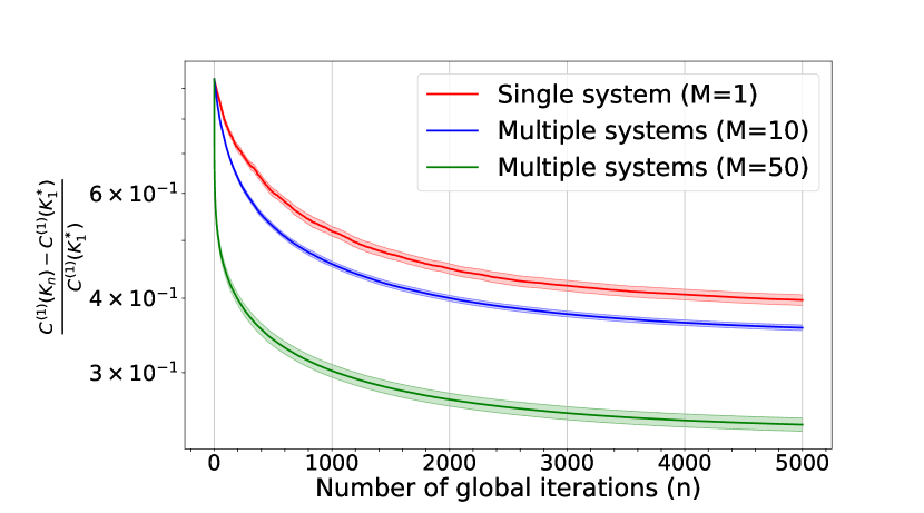
Figure 1: Gap between the current and optimal cost with respect to the number of global iterations. Varying the number of systems for a fixed heterogeneity level $\epsilon_{1}=0.5$, $\epsilon_{2}=0.5$.

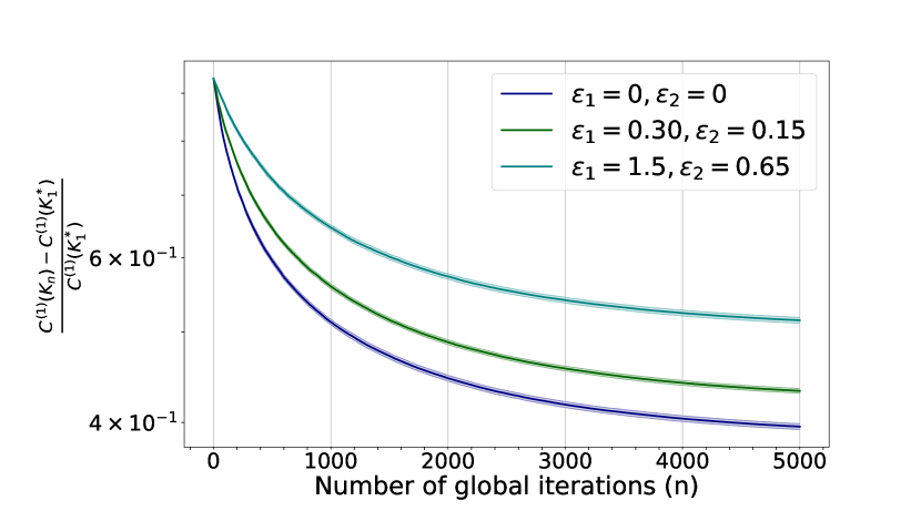
Figure 2: Gap between the current and optimal cost with respect to the number of global iterations. Varying the heterogeneity level among the systems, with a fixed number of systems $M=10$.

Figures 1 and 2 present the normalized distance between the current cost associated with the common stabilizing controller and the optimal cost for the nominal system, plotted with respect to the number of global iterations. These figures demonstrate the impact of varying the number of systems $M$ and the heterogeneity parameters $(\epsilon_{1},\epsilon_{2})$ on the convergence and performance of Algorithm 1.

In Figure 1, we specifically investigate the effect of the number of systems $M$ participating in the collaboration to compute a common controller $K^{*}$ on the convergence of our algorithm. In this analysis, we set the heterogeneity parameters as $\epsilon_{1}=0.5$ and $\epsilon_{2}=0.5$ and consider modification masks $Z_{1}=Z_{2}=I_{3}$. The figure reveals a noticeable reduction in the gap between the current and optimal cost as the number of participating systems $M$ increases. This numerical result aligns with our theoretical findings, which indicate that the number of samples required to achieve reliable estimation for the cost function’s gradient can be scaled down with the number of systems participating in the collaboration. Consequently, as the number of systems involved increases, there is a considerable reduction in the gap between the common computed controller and the optimal one.

Figure 2 illustrates the influence of the heterogeneity parameters $(\epsilon_{1},\epsilon_{2})$ on the convergence rate of Algorithm 1. In this analysis, we set the number of systems as $M=10$, and the modification masks $Z_{1}=\texttt{diag}([3.5\;\ 1\;\ 0.1])$ and $Z_{2}=\texttt{diag}([1.5\;\ 0.1\;\ 1])$. Consistent with our theoretical findings, we observe that an increase in the dissimilarity among the systems results in a significant gap between the common and optimal controller. This discrepancy arises due to the additive effect of system heterogeneity on the convergence rate of our algorithm, as elaborated in Theorem 5.

8 Conclusions and Future Work

We investigated the problem of learning a common and optimal LQR policy with the objective of minimizing an average quadratic cost. The primary focus of this paper was to thoroughly examine and provide comprehensive answers to the following questions: (i) Is the learned common policy stabilizing for all agents? (ii) How close is the learned common policy to each agent’s own optimal policy? (iii) Can each agent learn its own optimal policy faster by leveraging data from all agents? To address these questions, we proposed a federated and model-free approach, FedLQR, where $M$ heterogenous systems collaborate to learn a common and optimal policy while keeping the system’s data private. Our analysis tackles numerous technical challenges, including system heterogeneity, multiple local gradient descent updates, and stability. We have demonstrated that FedLQR produces a common policy that stabilizes (Theorem 5) all systems and converges to the optimal policy (Theorem 4) of each agent up to a heterogeneity bias term. Furthermore, FedLQR achieves a reduction in sample complexity proportional to the number of participating agents $M$ (Lemma 4). We also have provided numerical results to effectively showcase and evaluate the performance of our FedLQR approach in a model-free setting.

Future work will address the assumption of requiring full-state information to extend our results to the Linear Quadratic Gaussian (LQG) problem in a federated setting. We are currently investigating data-driven and system-theoretic metrics for heterogeneity, as well as personalization-based methods to mitigate the impact of system heterogeneity on the performance of the proposed approach.

Appendix

Appendix A Appendix Roadmap

This appendix is organized as follows. Section B offers a comprehensive and detailed overview of the relevant literature related to this paper. Sections C and D present important auxiliary norm inequalities and lemmas that play a key role in proving the main results of this paper. The proof of our main results related to the model-based setting is provided in Section E, while Section G is dedicated to the corresponding results in the model-free setting. Additional details on the zeroth-order optimization method are provided in Section F.

A.1 Notation Recap

For convenience we briefly recap and summarize our notation. We use $\|S\|_{max}$ to denote the maximum spectral norm taken over the family of matrices $S^{(1)},\ldots,S^{(M)}$. All norms for matrices and vectors are spectral and Euclidean respectively, unless otherwise stated. The integer sequence $1,2,\ldots,N$ is denoted as $[N]$. The spectral radius of a square matrix is denoted by $\rho(\cdot)$.

Symbol		Meaning
$M$		number of systems
$L$		number of local updates (counter: $l$)
$N$		number of rounds of averaging (counter: $n$)
$K_{n}$		averaged controller at round $n$
$K_{i}^{*}$		optimal controller for system $(A^{(i)},B^{(i)})$
$K_{n,l}^{(i)}$		controller for system $i$ after $l$ local iterations and $n$ averaging rounds

Appendix B Related Work

This section provides a more detailed and comprehensive literature survey on the key topics closely related to the subject matter of this paper. We aim to explore and summarize the main ideas presented in the existing literature pertaining to federated learning (FL), policy gradient (PG), federated reinforcement learning (FRL), as well as model-based and model-free linear quadratic control.

• Federated Learning (FL):

  In this work, we employ the federated learning (FL) paradigm to facilitate collaborative learning among systems without the need to share raw data with other participants or a server (Konečnỳ et al., 2016a; McMahan et al., 2017; Konečnỳ et al., 2016b; Bonawitz et al., 2019). Despite FL being a relatively recent creation, it has already garnered significant attention and boasts a wealth of literature. Below we highlight work that is most relevant to our problem setting.

  Federated averaging (FedAvg) stands as the pioneering and most widely adopted algorithm in FL. Originally proposed by McMahan et al. in (McMahan et al., 2017), FedAvg has demonstrated its effectiveness in homogeneous settings (Stich, 2018; Wang and Joshi, 2021; Spiridonoff et al., 2020; Reisizadeh et al., 2020; Haddadpour et al., 2019) where all participating clients aim to minimize the same objective function. However, ensuring convergence guarantees for FedAvg becomes notably more challenging in the presence of heterogeneity (Khaled et al., 2019b, 2020; Haddadpour and Mahdavi, 2019; Li et al., 2019b), thus necessitating additional assumptions on the gradient and Hessian dissimilarity bounds (Li et al., 2019b; Li and Orabona, 2019; Khaled et al., 2019b; Karimireddy et al., 2020). This difficulty arises primarily due to a "client-drift" effect, which is inherent to the FedAvg algorithm and has a detrimental impact on its convergence performance (Charles and Konečnỳ, 2020b, 2021b). As a result of the challenges posed by FedAvg, several alternative algorithms have been proposed to address its limitations. Notable examples of these algorithms include FedProx (Li et al., 2020), Scaffold (Karimireddy et al., 2020), FedSplit (Pathak and Wainwright, 2020b), FedDR (Tran Dinh et al., 2021), FedADMM (Wang et al., 2022a), FedLin (Mitra et al., 2021), and S-Local-SVRG (Gorbunov et al., 2021). Each of them introduces unique techniques and modifications to the original FedAvg algorithm, aiming to enhance convergence guarantees while handling communication cost concerns, statistical heterogeneity, client dropout, and sample complexity more effectively.

  Applying federated learning (FL) to control systems introduces a novel research direction that comes with its own set of challenges. Control systems exhibit unique characteristics, such as non-iid and non-isotropic data, as well as system instability, which arise due to the dynamic nature of the systems. These characteristics pose specific challenges when attempting to leverage data from multiple systems for tasks such as system identification (Wang et al., 2022b) or control synthesis (Ren et al., 2020).

  Although Ren et al. (2020) addresses the model-free LQR tracking problem in a federated manner, it focuses on a significantly simpler scenario where all agents follow identical dynamics (i.e., no heterogeneity). In contrast, our present work introduces new analysis techniques to achieve linear speedup in FedLQR when dealing with heterogeneous dynamical systems and multiple local updates per communication round.

• Policy Gradient (PG):

  The policy gradient (PG) approach is a fundamental component of the success of reinforcement learning (RL) and plays a crucial role in policy optimization (PO). This approach directly optimizes the policy to improve system-level performances through gradient ascent steps. The concept of policy optimization has been influential in RL (Sutton et al., 1999) with some well-known algorithms such as REINFORCE (Williams, 1992), trust-region policy optimization TRPO (Schulman et al., 2015), actor-critic methods (Konda and Tsitsiklis, 1999), and proximal policy optimization PPO (Schulman et al., 2017). We highlight an important difference between standard MDP models and control models in RL. In control, one requires the policy to provide closed-loop stability, i.e., all trajectories of the system must converge for a given policy. In contrast, convergence in the MDP setting requires irreducibly and aperiodicity properties that are assumed before a policy is selected. As a result, the control task is significantly more challenging.

  The extensive body of literature on policy optimization for reinforcement learning (RL) and its adaptability to the model-free setting paves the way for leveraging policy gradient methods in the pursuit of learning optimal control policies for classical control problems (Hu et al., 2022; Perdomo et al., 2021). Despite the non-convex nature of the formulation involved in policy gradient methods, recent work (Fazel et al., 2018; Malik et al., 2019; Hambly et al., 2021; Mohammadi et al., 2021; Gravell et al., 2020; Jin et al., 2020; Ju et al., 2022; Perdomo et al., 2021; Lamperski, 2020) has demonstrated global convergence in solving the model-free LQR problem via policy gradient methods. This convergence is achieved due to certain properties of the quadratic cost function inherent in the LQR problem as introduced in (Fazel et al., 2018). In contrast to the aforementioned work, which exclusively focus on the centralized control setting, our paper offers convergence guarantees for the multi-agent setting. In this context, each agent follows similar, but not identical, dynamics, thereby distinguishing it from the simpler scenario in (Ren et al., 2020).

• Federated Reinforcement Learning (FRL):

  The flexibility of policy gradient methods in the model-free RL setting has paved the way for a relatively recent research direction known as federated reinforcement learning (FRL), which aims to address practical implementation challenges of RL through the use of federated learning (Qi et al., 2021). FRL focuses on learning a common value function (Wang et al., 2023; Fabbro et al., 2023) or improving the policy by leveraging multiple RL agents interacting with similar environments. The empirical evidence presented in the survey paper (Qi et al., 2021) demonstrates the significant success of FRL in reducing sample complexity across various applications such as autonomous driving (Liang et al., 2022), IoT devices (Lim et al., 2020), resource management in networking (Yu et al., 2020), and communication efficiency (Gatsis, 2022). However, it is important to note that existing recent works in this field do not specifically tackle the challenge of finding a common and stabilizing optimal policy that is suitable for all RL agents in a heterogeneous setting.

• Model-free Linear Quadratic Control:

  The linear quadratic regulator (LQR) problem is a well-studied classical control problem that has gained significant attention due to its wide applicability and its role as a baseline for more complex control strategies (Anderson and Moore, 2007). Recently, to address the non-convex nature of the policy gradient LQR, (Sun and Fazel, 2021) has proposed convexifying the corresponding optimal control problem to efficiently solve the model-based LQR problem via policy gradient. Furthermore, the model-free LQR has attracted considerable interest after (Fazel et al., 2018) provided guarantees on the global convergence of policy gradient methods for both model-based and model-free LQR settings. This breakthrough paved the way for subsequent works (Malik et al., 2019; Hambly et al., 2021; Mohammadi et al., 2021; Gravell et al., 2020; Jin et al., 2020; Ju et al., 2022; Perdomo et al., 2021; Lamperski, 2020) that analyze convergence guarantees and sample complexity in the context of the model-free LQR problem. Notably, (Dean et al., 2020) characterizes the sample complexity of the LQR problem.

  Another line of work explores certainty equivalent control (Mania et al., 2019; Simchowitz and Foster, 2020), providing regret bounds to demonstrate the quality of the designed linear quadratic regulator in terms of the accuracy of the estimated system model. However, the key distinction between these works and the present paper lies in the consideration of multiple and heterogeneous systems. Moreover, (Mania et al., 2019; Simchowitz and Foster, 2020) use the regret framework, which is different from the PAC learning-based framework (Fiechter, 1997) exploited in our paper.

Appendix C Useful Norm Inequalities

• Given any two matrices $A,B$ of the same dimensions, for any $\xi>0$, we have

  $$\|A+B\|_{F}^{2}\leq(1+\xi)\|A\|_{F}^{2}+\left(1+\frac{1}{\xi}\right)\|B\|_{F}^{2}.$$ (6)

• Given any two matrices $A,B$ of the same dimensions, for any $\xi>0$, we have

  $$\langle A,B\rangle\leq\frac{\xi}{2}\lVert A\rVert_{F}^{2}+\frac{1}{2\xi}\lVert B\rVert_{F}^{2}.$$ (7)

  This inequality goes by the name of Young’s inequality.

• Given $m$ matrices $A_{1},\ldots,A_{m}$ of the same dimensions, the following is a simple application of Jensen’s inequality:

  $$\left\|\sum_{i=1}^{m}A_{i}\right\|^{2} \leq m\sum_{i=1}^{m}\left\|A_{i}\right\|^{2},$$

  $$\left\|\sum_{i=1}^{m}A_{i}\right\|_{F}^{2} \leq m\sum_{i=1}^{m}\left\|A_{i}\right\|_{F}^{2}.$$ (8)

• Given any two vectors $x,y\in\mathbb{R}^{d}$, for any constant $\zeta>0$, we have

  $$\|x+y\|^{2}\leq(1+\zeta)\|x\|^{2}+\left(1+\frac{1}{\zeta}\right)\|y\|^{2}.$$ (9)

• Given any two vectors $x,y\in\mathbb{R}^{d}$, for any constant $\zeta>0$, we have

  $$\langle x,y\rangle\leq\frac{\zeta}{2}\lVert x\rVert^{2}+\frac{1}{2\zeta}\lVert y\rVert^{2}.$$ (10)

Appendix D Useful Lemmas and Constants

Lemma 5.

For each $i\in[M],$ we have that:

$$||\Sigma^{(i)}_{K}||\leq\frac{{C}^{(i)}(K)}{\sigma_{\text{min}}(Q)},\quad||P^{(i)}_{K}||\leq\frac{C^{(i)}(K)}{\mu}.$$ (11)

Proof: The proof of this lemma is explained in detail in the proof of Lemma 13 of the supplemental materials in (Fazel et al., 2018). $\hfill\Box$

Lemma 6.

(Uniform bounds for $\nabla C(K)$ and $||K||$) For each agent $i\in[M]$, the gradient $\nabla C^{(i)}(K)$ and $\|K\|$ can be bounded as follows:

$$\|\nabla C^{(i)}(K)\|\leq\|\nabla C^{(i)}(K)\|_{F}\leq h_{1}(K)\quad\text{and}\quad\|K\|\leq h_{2}(K),$$

where $h_{1}(K)$, and $h_{2}(K)$ are some positive scalars depending on the function $C(K)$.

Proof: In this Lemma, $h_{1}(K)$, and $h_{2}(K)$ are the functions defined as:

$$h_{0}(K):=\sqrt{\frac{\left\|R_{K}\right\|_{\max}\left(C_{\max}(K)-C_{\min}\left(K\right)\right)}{\mu}},$$

$$h_{1}(K):=\frac{C_{\max}(K)h_{0}(K)}{\sigma_{\min}(Q)},\quad h_{2}(K):=\frac{h_{0}(K)+\left\|B^{\top}P_{K}A\right\|_{\max}}{\sigma_{\min}(R)},$$

where $\|R_{K}\|_{\max}:=\max_{i}\left\|R+B^{(i)\top}P^{(i)}_{K}B^{(i)}\right\|.$ By using Lemma 13 of (Fazel et al., 2018), we have

$$\|\nabla C^{(i)}(K)\|^{2} \leq\operatorname{Tr}\left(\Sigma^{(i)}_{K}E^{(i)\top}_{K}E^{(i)}_{K}\Sigma^{(i)}_{K}\right)\leq\left\|\Sigma^{(i)}_{K}\right\|^{2}\operatorname{Tr}\left(E^{(i)\top}_{K}E^{(i)}_{K}\right)$$

$$\leq\left(\frac{C^{(i)}(K)}{\sigma_{\min}(Q)}\right)^{2}\operatorname{Tr}\left(E^{(i)\top}_{K}E^{(i)}_{K}\right).$$

By Lemma 11 of (Fazel et al., 2018), we obtain

$$\operatorname{Tr}\left(E^{(i)\top}_{K}E^{(i)}_{K}\right)\leq\frac{\left\|R+B^{(i)\top}P^{(i)}_{K}B^{(i)}\right\|\left(C^{(i)}(K)-C^{(i)}\left(K_{i}^{*}\right)\right)}{\mu},$$

which proves the first claim:

$$\|\nabla C^{(i)}(K)\| \leq\frac{C^{(i)}(K)}{\sigma_{\min}(Q)}\sqrt{\frac{\left\|R+B^{(i)\top}P^{(i)}_{K}B^{(i)}\right\|\left(C^{(i)}(K)-C^{(i)}\left(K_{i}^{*}\right)\right)}{\mu}}$$

$$\leq\frac{C_{\max}(K)}{\sigma_{\min}(Q)}\sqrt{\frac{\left\|R+B^{(i)\top}P^{(i)}_{K}B^{(i)}\right\|_{\max}\left(C_{\max}(K)-C_{\min}\left(K\right)\right)}{\mu}}.$$

On the other hand, by exploiting Lemma 11 of (Fazel et al., 2018) we can also write

$$\|K\| \leq\left\|\left(R+B^{(i)\top}P^{(i)}_{K}B^{(i)}\right)^{-1}\right\|\left\|\left(R+B^{(i)\top}P^{(i)}_{K}B^{(i)}\right)K\right\|$$

$$\leq\frac{1}{\sigma_{\min}(R)}\left\|\left(R+B^{(i)\top}P^{(i)}_{K}B^{(i)}\right)K\right\|$$

$$\leq\frac{1}{\sigma_{\min}(R)}\left(\left\|\left(R+B^{(i)\top}P^{(i)}_{K}B^{(i)}\right)K-B^{(i)\top}P^{(i)}_{K}A^{(i)}\right\|+\left\|B^{(i)\top}P^{(i)}_{K}A^{(i)}\right\|\right)$$

$$=\frac{\left\|E^{(i)}_{K}\right\|}{\sigma_{\min}(R)}+\frac{\left\|B^{(i)\top}P^{(i)}_{K}A^{(i)}\right\|}{\sigma_{\min}(R)}$$

$$\leq\frac{\sqrt{\operatorname{Tr}\left(E^{(i)\top}_{K}E^{(i)}_{K}\right)}}{\sigma_{\min}(R)}+\frac{\left\|B^{(i)\top}P^{(i)}_{K}A^{(i)}\right\|}{\sigma_{\min}(R)}$$

$$=\frac{\sqrt{\left(C^{(i)}(K)-C^{(i)}\left(K_{i}^{*}\right)\right)\left\|R+B^{(i)\top}P^{(i)}_{K}B^{(i)}\right\|}}{\sqrt{\mu}\sigma_{\min}(R)}+\frac{\left\|B^{(i)\top}P^{(i)}_{K}A^{(i)}\right\|}{\sigma_{\min}(R)},$$

which completes the proof for the second claim. $\hfill\Box$

It is worth noting that the local cost and gradient smoothness, and gradient domination properties in Lemma 1 and Lemma 2 not only hold for the single-agent setting but also hold for the multi-agent setting. Moreover, we will make use of the following matrix Martingale concentration inequality:

Lemma 7.

(Rectangular Matrix Freedman (Tropp, 2011)). Consider a matrix martingale $\left\{{Y}_{k}:k=0,1,2,\ldots\right\}$ whose values are matrices with dimension $d_{1}\times d_{2}$, and let $\left\{{X}_{k}:k=1,2,3,\ldots\right\}$ be the difference sequence. Assume that the difference sequence is uniformly bounded:

$$\left\|{X}_{k}\right\|\leq R\quad\text{ almost surely }\quad\text{ for }k=1,2,3,\ldots.$$

Define two predictable quadratic variation processes for this martingale:

$${W}_{\mathrm{col},k}:=\sum_{j=1}^{k}\mathbb{E}_{j-1}\left({X}_{j}{X}_{j}^{*}\right)\text{ and }$$

$${W}_{\text{row },k}:=\sum_{j=1}^{k}\mathbb{E}_{j-1}\left({X}_{j}^{*}{X}_{j}\right)\quad\text{ for }k=1,2,3,\ldots$$

Then, for all $t\geq 0$ and $\sigma^{2}>0$,

$$\mathbb{P}\left\{\exists k\geq 0:\left\|{Y}_{k}\right\|\geq t\text{ and }\max\left\{\left\|{W}_{\text{col },k}\right\|,\left\|{W}_{\text{row },k}\right\|\right\}\leq\sigma^{2}\right\}\leq\left(d_{1}+d_{2}\right)\cdot\exp\left\{-\frac{-t^{2}/2}{\sigma^{2}+Rt/3}\right\}.$$

D.1 Proof of Lemma 1

Proof: In this proof, we aim to show

$$\left|C^{(i)}\left(K^{\prime}\right)-C^{(i)}(K)\right| \leq h_{\text{cost}}(K)\|K^{\prime}-K\|,$$

$$\left\|\nabla C^{(i)}\left(K^{\prime}\right)-\nabla C^{(i)}(K)\right\|\leq h_{\text{grad }}(K)\|\Delta\| \text{ and }\left\|\nabla C^{(i)}\left(K^{\prime}\right)-\nabla C^{(i)}(K)\right\|_{F}\leq h_{\text{grad}}(K)\|\Delta\|_{F},$$

hold for all agents $i\in[M]$ and $K^{\prime}$ satisfying $\|K^{\prime}-K\|\leq h_{\Delta}(K)\ <\infty.$

The term $h_{\Delta}(K)$ is the polynomial defined as

$$h_{\Delta}(K):=\frac{\sigma_{\min}(Q)\mu}{4||B||_{\max}C_{\max}(K)\left(\left\|A-BK\right\|_{\max}+1\right)},$$

the term $h_{\text{cost }}(K)$ and $h_{\text{grad}}(K)$ are defined as

$$\begin{gathered}h_{\text{cost }}(K):=\frac{4\operatorname{Tr}\left(\Sigma_{0}\right)C_{\max}(K)\|R\|}{\mu\sigma_{\min}\left(Q\right)}\left(\|K\|+\frac{h_{\Delta}(K)}{2}+\|B\|_{\max}\|K\|^{2}\left(\left\|A-BK\right\|_{\max}+1\right)\frac{C_{\max}(K)}{\mu\sigma_{\min}(Q)}\right)\end{gathered}$$

$$h_{\text{grad }}(K) :=4\left(\frac{C_{\max}(K)}{\sigma_{\min}(Q)}\right)\Big{[}\|R\|+\|B\|_{\max}\left(\|A\|_{\max}+||B||_{\max}\left(\|K\|+h_{\Delta}(K)\right)\right)$$

$$\times\left(\frac{h_{\text{cost }}(K)C_{\max}(K)}{\operatorname{Tr}\left(\Sigma_{0}\right)}\right)+\|B\|^{2}_{\max}\frac{C_{\max}(K)}{\mu}\Big{]}$$

$$+8\left(\frac{C_{\max}(K)}{\sigma_{\min}(Q)}\right)^{2}\left(\frac{\|B\|_{\max}\left(\left\|A-BK\right\|_{\max}+1\right)}{\mu}\right)h_{0}(K).$$

For the single-agent (i.e., $M=1$) setting, the proof is explained in detail in the proof of Lemma 24 and Lemma 25 of the supplemental materials in (Fazel et al., 2018). For the multi-agent setting (i.e., $M>1$), we can complete the proof by taking the maximum over the clients $i\in[M]$ of all the system-dependent parameters, such as $\lVert B\rVert_{\max}.$ $\hfill\Box$

D.2 Proof of Lemma 2

Proof: For the single-agent (i.e., $M=1$) setting, the proof is explained in the proof of Lemma 11 of the supplemental materials in (Fazel et al., 2018). For the multi-agent setting (i.e., $M>1$), it is easy to see that

$$C^{(i)}(K)-C^{(i)}\left(K_{i}^{*}\right)\leq\frac{\left\|\Sigma_{K_{i}^{*}}\right\|}{4\mu^{2}\sigma_{\min}(R)}\|\nabla C^{(i)}(K)\|_{F}^{2}$$

holds for any stabilizing controller $K$ and any agent $i\in[M].$ $\hfill\Box$

Appendix E The model-based setting

We first introduce the following operators on a symmetric matrix $X$,

$$\mathcal{T}^{(i)}_{K}(X) :=\sum_{t=0}^{\infty}(A^{(i)}-B^{(i)}K)^{t}X\left[(A^{(i)}-B^{(i)}K)^{\top}\right]^{t},$$

$$\mathcal{F}^{(i)}_{K}(X) :=(A^{(i)}-B^{(i)}K)X(A^{(i)}-B^{(i)}K)^{\top}.$$ (12)

We also define the induced norms of $\mathcal{T}$ and $\mathcal{F}$ as

$$\left\|\mathcal{T}_{K}\right\|=\sup_{X}\frac{\left\|\mathcal{T}_{K}(X)\right\|}{\|X\|},\quad\left\|\mathcal{F}_{K}\right\|=\sup_{X}\frac{\left\|\mathcal{F}_{K}(X)\right\|}{\|X\|}.$$

Lemma 8.

When $(A^{(i)}-B^{(i)}K)$ has spectral radius smaller than 1, we have

$$\mathcal{T}_{K}^{(i)}=\left(\mathrm{I}-\mathcal{F}_{K}^{(i)}\right)^{-1}$$

holds for each $i\in[M].$

Proof: The proof is explained in detailed in the proof of Lemma 18 in Fazel et al. (2018). $\hfill\Box$

Lemma 9.

If

$$\left\|\mathcal{T}^{(i)}_{K}\right\|\left\|\mathcal{F}^{(i)}_{K}-\mathcal{F}^{(j)}_{K}\right\|\leq\frac{1}{2}$$ (13)

holds for any system $i,j\in[M],$ then we have

$$\left\|\left(\mathcal{T}^{(i)}_{K}-\mathcal{T}^{(j)}_{K}\right)(X)\right\| \leq 2\left\|\mathcal{T}^{(i)}_{K}\right\|\left\|\mathcal{F}^{(i)}_{K}-\mathcal{F}^{(j)}_{K}\right\|\left\|\mathcal{T}^{(i)}_{K}(X)\right\|$$

$$\leq 2\left\|\mathcal{T}^{(i)}_{K}\right\|^{2}\left\|\mathcal{F}^{(i)}_{K}-\mathcal{F}_{K}^{(j)}\right\|\|\ X\|.$$

Proof: Define $\mathcal{A}=\mathrm{I}-\mathcal{F}^{(i)}_{K}$, and $\mathcal{B}=\mathcal{F}^{(i)}_{K}-\mathcal{F}^{(j)}_{K}$. In this case $\mathcal{A}^{-1}=\mathcal{T}^{(i)}_{K}$ and $(\mathcal{A}-\mathcal{B})^{-1}=\mathcal{T}^{(j)}_{K}$. Hence, the condition $\left\|\mathcal{T}^{(i)}_{K}\right\|\left\|\mathcal{F}^{(i)}_{K}-\mathcal{F}^{(j)}_{K}\right\|\leq\frac{1}{2}$ translates to the condition $\left\|\mathcal{A}^{-1}\right\|\|\mathcal{B}\|\leq\frac{1}{2}$.

First, we observe that

$$\left(\mathcal{A}^{-1}-(\mathcal{A}-\mathcal{B})^{-1}\right)(X)=\left(\mathrm{I}-\left(\mathrm{I}-\mathcal{A}^{-1}\circ\mathcal{B}\right)^{-1}\right)\left(\mathcal{A}^{-1}(X)\right)=\left(\mathrm{I}-\left(\mathrm{I}-\mathcal{A}^{-1}\circ\mathcal{B}\right)^{-1}\right)\left(\mathcal{T}^{(i)}_{K}(X)\right),$$ (14)

where $f\circ g$ denotes the composition $f(g(x))$. Since $\left(\mathrm{I}-\mathcal{A}^{-1}\circ\mathcal{B}\right)^{-1}=\mathrm{I}+\mathcal{A}^{-1}\circ\mathcal{B}\circ\left(\mathrm{I}-\mathcal{A}^{-1}\circ\mathcal{B}\right)^{-1}$, we have:

$$\left\|\left(\mathrm{I}-\mathcal{A}^{-1}\circ\mathcal{B}\right)^{-1}\right\|\leq 1+\left\|\mathcal{A}^{-1}\circ\mathcal{B}\right\|\left\|\left(\mathrm{I}-\mathcal{A}^{-1}\circ\mathcal{B}\right)^{-1}\right\|\leq 1+\frac{1}{2}\left\|\left(\mathrm{I}-\mathcal{A}^{-1}\circ\mathcal{B}\right)^{-1}\right\|$$ (15)

Now rearranging terms in Eq.(15), we obtain $\left\|\left(\mathrm{I}-\mathcal{A}^{-1}\circ\mathcal{B}\right)^{-1}\right\|\leq 2$. Therefore, we have

$$\left\|\mathrm{I}-\left(\mathrm{I}-\mathcal{A}^{-1}\circ\mathcal{B}\right)^{-1}\right\|=\left\|\mathcal{A}^{-1}\circ\mathcal{B}\circ\left(\mathrm{I}-\mathcal{A}^{-1}\circ\mathcal{B}\right)^{-1}\right\| \leq\left\|\mathcal{A}^{-1}\right\|\|\mathcal{B}\|\left\|\left(\mathrm{I}-\mathcal{A}^{-1}\circ\mathcal{B}\right)^{-1}\right\|$$

$$\leq 2\left\|\mathcal{A}^{-1}\right\|\|\mathcal{B}\|,$$

and so

$$\left\|\mathrm{I}-\left(\mathrm{I}-\mathcal{A}^{-1}\circ\mathcal{B}\right)^{-1}\right\|\leq 2\left\|\mathcal{A}^{-1}\right\|\|\mathcal{B}\|=2\left\|\mathcal{T}^{(i)}_{K}\right\|\left\|\mathcal{F}^{(i)}_{K}-\mathcal{F}^{(j)}_{K}\right\|.$$ (16)

Then, we have

$$\left\|\left(\mathcal{T}^{(i)}_{K}-\mathcal{T}^{(j)}_{K}\right)(X)\right\| =\left\|\left(\mathcal{A}^{-1}-(\mathcal{A}-\mathcal{B})^{-1}\right)(X)\right\|$$

$$\stackrel{{\scriptstyle(a)}}{{\leq}}\left\|\left(\mathrm{I}-\left(\mathrm{I}-\mathcal{A}^{-1}\circ\mathcal{B}\right)^{-1}\right)\right\|\left\|\mathcal{T}^{(i)}_{K}(X)\right\|$$

$$\stackrel{{\scriptstyle(b)}}{{\leq}}2\left\|\mathcal{T}^{(i)}_{K}\right\|\left\|\mathcal{F}^{(i)}_{K}-\mathcal{F}^{(j)}_{K}\right\|\left\|\mathcal{T}^{(i)}_{K}(X)\right\|$$

$$\leq 2\left\|\mathcal{T}^{(i)}_{K}\right\|\left\|\mathcal{F}^{(i)}_{K}-\mathcal{F}^{(j)}_{K}\right\|\left\|\mathcal{T}^{(i)}\right\|\left\|X\right\|,$$

where $(a)$ is due to Eq.(14) and $(b)$ is due to Eq.(16). This completes the proof of Lemma 9. $\hfill\Box$.

E.1 Proof of Lemma 3

Proof: First, we know that $\nabla C^{(i)}(K)$ and $\nabla C^{(j)}(K)$ are given by,

$$\nabla C^{(i)}(K)=2E^{(i)}_{K}\Sigma^{(i)}_{K},\quad\text{and}\quad\nabla C^{(j)}(K)=2E^{(j)}_{K}{\Sigma}^{(j)}_{K}$$

where,

$$E^{(i)}_{K} =(R+B^{(i)\top}P^{(i)}_{K}B^{(i)})K-B^{(i)\top}P^{(i)}_{K}A^{(i)},$$

and

$$\Sigma^{(i)}_{K}=_{x^{(i)}_{0}\sim D}\sum_{t=0}^{\infty}x^{(i)}_{t}x^{(i)\top}_{t}.$$

Thus, we can write,

$$||\nabla C^{(i)}(K)-\nabla C^{(j)}(K)|| =||2E^{(i)}_{K}\Sigma^{(i)}_{K}-2E^{(j)}_{K}\Sigma^{(j)}_{K}||$$

$$\leq 2(||E^{(i)}_{K}-E^{(j)}_{K}||\underbrace{||\Sigma^{(i)}_{K}||}_{\beta_{1}}+\underbrace{||E^{(j)}_{K}||}_{\beta_{2}}||\Sigma^{(i)}_{K}-\Sigma^{(j)}_{K}||).$$

From Eq. (11) we can upper bound $||\Sigma^{(i)}_{K}||$ as:

$$||\Sigma^{(i)}_{K}||\leq\frac{{C}^{(i)}(K)}{\sigma_{\text{min}}(Q)}.$$

With the definition of $E^{(j)}_{K}=RK+B^{(j)\top}P^{(j)}_{K}B^{(j)}K-B^{(j)\top}P^{(j)}_{K}A^{(j)}$, we can use triangle inequality to write,

$$||E^{(j)}_{K}|| \leq||RK||+||B^{(j)}||||P^{(j)}_{K}||||B^{(j)}K||+||B^{(j)}||||P^{(j)}_{K}||||A^{(j)}||$$

$$\leq||RK||+\frac{||B^{(j)}||C^{(j)}(K)}{{\mu}}(||B^{(j)}K||+||A^{(j)}||),$$

where $||P^{(j)}_{K}||\leq\frac{C^{(j)}(K)}{\mu}$ from Eq. (11), with $\mu=\sigma_{\min}({\Sigma}^{(j)}_{0})$.

With the notation that we introduced previously, we can write

$$\beta_{1}=||\Sigma^{(i)}_{K}||\leq||\Sigma_{K}||_{\max}\leq\frac{{C_{\max}}(K)}{\sigma_{\min}(Q)},$$

and,

$$\beta_{2}=||E^{(j)}_{K}||\leq||E_{K}||_{\max}\leq||R||||K||+\frac{||B||_{\max}C_{\max}(K)}{{\mu}}(||B||_{\max}+||A||_{\max}),$$

where $C_{\max}(K):=\max_{i}C^{(i)}(K)$.

Next we will derive an upper bound for $||E^{(i)}_{K}-E^{(j)}_{K}||$.

Upper bound for $||E^{(i)}_{K}-E^{(j)}_{K}||$: We can first use the definition of $E_{K}^{(i)}$ and $E^{(j)}_{K}$ to write,

$$E^{(i)}_{K} -E^{(j)}_{K}=B^{(j)\top}P^{(j)}_{K}(A^{(j)}-B^{(j)}K)-B^{(i)\top}P^{(i)}_{K}(A^{(i)}-B^{(i)}K)$$

$$=-B^{(i)\top}P^{(i)}_{K}(A^{(i)}-B^{(i)}K)+B^{(i)\top}P^{(i)}_{K}(A^{(j)}-B^{(j)}K)-B^{(i)\top}P^{(i)}_{K}(A^{(j)}-B^{(j)}K)$$

$$+B^{(i)\top}P^{(j)}_{K}(A^{(j)}-B^{(j)}K)-B^{(i)\top}P^{(j)}_{K}(A^{(j)}-B^{(j)}K)+B^{(j)\top}P^{(j)}_{K}(A^{(j)}-B^{(j)}K).$$

Then, by using triangle inequality, we obtain the following expression:

$$||E^{(i)}_{K}-E^{(j)}_{K}|| \leq||\underbrace{B^{(i)\top}P^{(i)}_{K}(A^{(i)}-B^{(i)}K)-B^{(i)\top}P^{(i)}_{K}(A^{(j)}-B^{(j)}K)}_{H_{1}}||$$

$$+||\underbrace{B^{(i)\top}P^{(i)}_{K}(A^{(j)}-B^{(j)}K)-B^{(i)\top}P^{(j)}_{K}(A^{(j)}-B^{(j)}K)}_{H_{2}}||$$

$$+||\underbrace{B^{(i)\top}P^{(j)}_{K}(A^{(j)}-B^{(j)}K)-B^{(j)\top}P^{(j)}_{K}(A^{(j)}-B^{(j)}K)}_{H_{3}}||.$$

Incorporating the heterogeneity bounds from assumption 1 gives

$$||H_{1}||\leq||B^{(i)}||||P^{(i)}_{K}||(\epsilon_{1}+\epsilon_{2}||K||),$$

to which we apply the max-norm definition to arrive at

$$||H_{1}||\leq||B||_{\max}(\epsilon_{1}+\epsilon_{2}||K||)||P_{K}||_{\max}.$$ (17)

Similarly, we can also derive upper bounds for $||H_{2}||$ and $||H_{3}||$, as follows,

$$||H_{2}||\leq||B^{(i)}||||P^{(i)}_{K}-P^{(j)}_{K}||||A^{(j)}-B^{(j)}K||\leq||B||_{\max}||P^{(i)}_{K}-P^{(j)}_{K}||||A-BK||_{\max}$$ (18)

and

$$||H_{3}||\leq\epsilon_{2}||A^{(i)}-B^{(i)}K||||P^{(j)}_{K}||\leq\epsilon_{2}||A-BK||_{\max}||P_{K}||_{\max}.$$ (19)

To bound $H_{2}$, we need to derive an upper bound for $||P^{(i)}_{K}-P^{(j)}_{K}||$. For this purpose, we have that for any fixed system $i\in[M]$

$$||P^{(i)}_{K}-P^{(j)}_{K}||=\left\|\mathcal{T}^{(i)}_{K}\left(Q+K^{\top}RK\right)-\mathcal{T}^{(j)}_{K}\left(Q+K^{\top}RK\right)\right\|.$$

Thus, by using Lemma 9, we can write,

$$||P^{(i)}_{K}-P^{(j)}_{K}||\leq 2\left\|\mathcal{T}^{(i)}_{K}\right\|^{2}\left\|\mathcal{F}^{(i)}_{K}-\mathcal{F}_{K}^{(j)}\right\|\left\|Q+K^{\top}RK\right\|,$$

where $||\mathcal{T}^{(i)}_{K}||\leq\frac{C^{(i)}(K)}{\sigma_{\min}(Q)\mu}\leq\frac{C_{\max}(K)}{\sigma_{\min}(Q)\mu}$ (detailed in Lemma 17 of (Fazel et al., 2018)). With the following upper bound for $\left\|\mathcal{F}^{(i)}_{K}-\mathcal{F}_{K}^{(j)}\right\|$:

$$||(\mathcal{F}^{(i)}_{K}-\mathcal{F}_{K}^{(j)})(X)|| =||(A^{(i)}-B^{(i)}K)X(A^{(i)}-B^{(i)}K)^{\top}$$

$$-(A^{(j)}-B^{(j)}K)X(A^{(j)}-B^{(j)}K)^{\top}||$$

$$\leq 2(\epsilon_{1}+\epsilon_{2}||K||)||X||||A-BK||_{\max},$$

we have

$$||P^{(i)}_{K}-P^{(j)}_{K}||\leq 4\left(\frac{C_{\max}(K)}{\sigma_{\min}(Q)\mu}\right)^{2}(\epsilon_{1}+\epsilon_{2}||K||)||A-BK||_{\max}(||Q||+||R||||K||^{2}),$$ (20)

Plugging in Eq. (20) into $H_{2}$ and adding the upper bounds of $H_{1}$ (Eq. 17), $H_{2}$ (Eq. 18) and $H_{3}$ (Eq. 19) together, we have

$$||E^{(i)}_{K}-E^{(j)}_{K}|| \leq g_{1}(\epsilon_{1},\epsilon_{2},K),$$

where $g_{1}$ is a linear in $\epsilon_{1},\epsilon_{2}$ and polynomial in the remaining problem data. Specifically,

$\displaystyle g_{1}(\epsilon_{1},\epsilon_{2},K)=\epsilon_{1}\left(\frac{||B||_{\max}C_{\max}(K)}{\mu}\left[1+4\left(\frac{C_{\max}(K)}{\sigma_{\min}(Q)\mu}\right)\left(||A-BK||_{\max}\right)^{2}\left(||Q||+||R||||K||^{2}\right)\right]\right)$ $\displaystyle+\epsilon_{2}\left(\frac{||B||_{\max}||K||C_{\max}(K)}{\mu}\left[1+4\left(\frac{C_{\max}(K)}{\sigma_{\min}(Q)\mu}\right)\left(||A-BK||_{\max}\right)^{2}\left(||Q||+||R||||K||^{2}\right)\right]+||A-BK||_{\max}\right).$

In what follows, we will derive an upper bound for $||\Sigma^{(i)}_{K}-\Sigma^{(j)}_{K}||$:

Upper bound for $||\Sigma^{(i)}_{K}-\Sigma^{(j)}_{K}||$: From the previous definitions in Eq.(E) and Lemma 9, we have,

$$||\Sigma^{(i)}_{K}-\Sigma^{(j)}_{K}|| =||\mathcal{T}^{(i)}_{K}(\Sigma_{0})-\mathcal{T}^{(j)}_{K}(\Sigma_{0})||\leq 2\left\|\mathcal{T}^{(i)}_{K}\right\|^{2}\left\|\mathcal{F}^{(i)}_{K}-\mathcal{F}_{K}^{(j)}\right\|\|\ \Sigma_{0}\|$$

$$\leq 4\left(\frac{C_{\max}}{\sigma_{\min}(Q)\mu}\right)^{2}(\epsilon_{1}+\epsilon_{2}||K||)||A-BK||_{\max}||\Sigma_{0}||$$

where $\Sigma_{0}=\mathbb{E}_{x_{0}^{(i)}\sim\mathcal{D}}\left[x_{0}^{(i)}x_{0}^{(i)\top}\right].$

Thus, we have the following upper bound for $||\Sigma^{(i)}_{K}-\Sigma^{(j)}_{K}||$,

$$||\Sigma^{(i)}_{K}-\Sigma^{(j)}_{K}||\leq g_{2}(\epsilon_{1},\epsilon_{2},K)$$

with,

$\displaystyle g_{2}(\epsilon_{1},\epsilon_{2},K)$ $\displaystyle=\epsilon_{1}\left(\frac{C_{\max}(K)}{\sigma_{\min}(Q)\mu}\right)^{2}\left(4||A-BK||_{\max}||\Sigma_{0}||\right)+\epsilon_{2}||K||\left(\frac{C_{\max}(K)}{\sigma_{\min}(Q)\mu}\right)^{2}\left(4||A-BK||_{\max}||\Sigma_{0}||\right).$

Therefore, we can finally write an upper bound for $||\nabla C^{(i)}(K)-\nabla C^{(j)}(K)||$, which is:

$$||\nabla C^{(i)}(K)-\nabla C^{(j)}(K)||\leq f(\epsilon_{1},\epsilon_{2},K)$$

where,

$$f(\epsilon_{1},\epsilon_{2},K)=2(\beta_{1}g_{1}(\epsilon_{1},\epsilon_{2},K)+\beta_{2}g_{2}(\epsilon_{1},\epsilon_{2},K)).$$

After some rearrangement, we have that

$$f(\epsilon_{1},\epsilon_{2},K)=\epsilon_{1}h^{1}_{\text{het}}(K)+\epsilon_{1}h^{2}_{\text{het}}(K),$$

where $h^{1}_{\text{het}}=h_{1f}+h_{2f}$ and $h^{2}_{\text{het}}=h_{3f}+h_{4f}$, and

$$h_{1f}=\frac{2||B||_{\max}(C_{\max}(K))^{2}}{\sigma_{\min}(Q)\mu}\left[1+4\left(\frac{C_{\max}(K)}{\sigma_{\min}(Q)\mu}\right)\left(||A-BK||_{\max}\right)^{2}\left(||Q||+||R||||K||^{2}\right)\right],$$

$$h_{2f}=\frac{2}{\mu}\left(\frac{C_{\max}(K)}{\sigma_{\min}(Q)}\right)^{3}\left(4||A-BK||_{\max}||\Sigma_{0}||\right),$$

$$h_{3f}=2\left(||R||||K||+\frac{||B||_{\max}C_{\max}(K)}{{\mu}}(||B||_{\max}+||A||_{\max})\right)$$

$$\times\left(\frac{||B||_{\max}||K||C_{\max}(K)}{\mu}\left[1+4\left(\frac{C_{\max}(K)}{\sigma_{\min}(Q)\mu}\right)\left(||A-BK||_{\max}\right)^{2}\left(||Q||+||R||||K||^{2}\right)\right]+||A-BK||_{\max}\right),$$

$$h_{4f}=2\left(||R||||K||+\frac{||B||_{\max}C_{\max}(K)}{{\mu}}(||B||_{\max}+||A||_{\max}\right)||K||\left(\frac{C_{\max}(K)}{\sigma_{\min}(Q)\mu}\right)^{2}\left(4||A-BK||_{\max}||\Sigma_{0}||\right).$$

E.2 Proof of Theorem 3

In this theorem, we consider the setting where $(\epsilon_{1}\bar{h}^{1}_{\text{het}}+\epsilon_{2}\bar{h}^{2}_{\text{het}})^{2}\leq\bar{h}^{3}_{\text{het}}$ with

$$\bar{h}^{3}_{\text{het}}:=\min_{j\in[M]}\left\{\frac{\mu^{2}\sigma_{\min}(R)\left(C^{(j)}(K_{0})-C^{(j)}(K_{j}^{*})\right)}{4||\Sigma_{K_{j}^{*}}||\min\{n_{x},n_{u}\}}\right\}.$$ (21)

Outline:

To prove Theorem 3, we first introduce some lemmas: Lemma 10 establishes stability of the local policies; Lemma 11 provides the drift analysis; Lemma 12 quantifies the per-round progress of our FedLQR algorithm. As a result, we are able to present the iterative stability guarantees and convergence analysis of FedLQR in the model-based setting.

Lemma 10.

(Stability of the local policies) Suppose $K_{n}\in\mathcal{G}^{0}.$ If the local step-size satisfies $\eta_{l}\leq\min\{\frac{\underline{h}_{\Delta}}{\bar{h}_{1}},\frac{1}{4\bar{h}_{\text{grad}}}\}$ and the heterogeneity level satisfies $(\epsilon_{1}\bar{h}^{1}_{\text{het}}+\epsilon_{2}\bar{h}^{2}_{\text{het}})^{2}\leq\bar{h}^{3}_{\text{het}}$, then $K_{n,l}^{(i)}\in\mathcal{G}^{0}$ holds for all $i\in[M]$ and $l\in[L]$.

Proof: Since $K_{n}\in\mathcal{G}^{0},$ based on the local Lipschitz property in Lemma 1, we have:

$$C^{(j)}(K_{n,1}^{(i)})-C^{(j)}(K_{n}) \leq\left\langle\nabla C^{(j)}(K_{n}),K_{n,1}^{(i)}-K_{n}\right\rangle+\frac{h_{\text{grad}}(K_{n})}{2}\Big{\lVert}K_{n,1}^{(i)}-K_{n}\Big{\rVert}_{F}^{2}\quad$$

$$\leq-\left\langle\nabla C^{(j)}(K_{n}),\eta_{l}{\nabla}C^{(i)}(K_{n})\right\rangle+\frac{h_{\text{grad}}(K_{n})}{2}\Big{\lVert}\eta_{l}{\nabla}C^{(i)}(K_{n})\Big{\rVert}_{F}^{2}$$ (22)

holds for any $i,j\in[M],$ if $\Big{\lVert}\eta_{l}{\nabla}C^{(i)}(K_{n})\Big{\rVert}_{F}\leq\underline{h}_{\Delta}\leq h_{\Delta}(K_{n}),$ which holds when

$$\Big{\lVert}\eta_{l}{\nabla}C^{(i)}(K_{n})\Big{\rVert}_{F}\stackrel{{\scriptstyle(a)}}{{\leq}}\eta_{l}h_{1}(K_{n})\leq\eta_{l}\bar{h}_{1}\stackrel{{\scriptstyle(b)}}{{\leq}}\underline{h}_{\Delta},$$

where $(a)$ comes from Lemma 6 and $(b)$ holds because of the requirement on $\eta_{l}$ in the statement of the lemma.

Following the analysis in Eq (E.2), we have

$$C^{(j)}(K_{n,1}^{(i)})-C^{(j)}(K_{n}) \leq-\eta_{l}\left\langle\nabla C^{(j)}(K_{n}),\nabla C^{(j)}(K_{n})\right\rangle$$

$$-\eta_{l}\underbrace{\left\langle\nabla C^{(j)}(K_{n}),\nabla C^{(i)}(K_{n})-\nabla C^{(j)}(K_{n})\right\rangle}_{T_{1}}$$

$$+\frac{h_{\text{grad}}(K_{n})}{2}\Big{\lVert}\eta_{l}{\nabla}C^{(i)}(K_{n})\Big{\rVert}_{F}^{2}.$$ (23)

Now $T_{1}$ can be bounded as

$$T_{1} \leq\eta_{l}\Big{\lVert}\nabla C^{(j)}(K_{n})\Big{\rVert}_{F}\Big{\lVert}\nabla C^{(i)}(K_{n})-\nabla C^{(j)}(K_{n})\Big{\rVert}_{F}$$

$$\leq\eta_{l}\sqrt{\min\{n_{x},n_{u}\}}\Big{\lVert}\nabla C^{(j)}(K_{n})\Big{\rVert}_{F}\Big{\lVert}\nabla C^{(i)}(K_{n})-\nabla C^{(j)}(K_{n})\Big{\rVert}$$

$$\stackrel{{\scriptstyle(c)}}{{\leq}}\eta_{l}\sqrt{\min\{n_{x},n_{u}\}}\Big{\lVert}\nabla C^{(j)}(K_{n})\Big{\rVert}_{F}(\epsilon_{1}\bar{h}^{1}_{\text{het}}+\epsilon_{2}\bar{h}^{2}_{\text{het}}),$$ (24)

where $(c)$ is due to Lemma 3. Plugging in the upper bound of $T_{1}$ into  (E.2), we have:

$$C^{(j)}(K_{n,1}^{(i)}) -C^{(j)}(K_{n})\leq-\eta_{l}\left\langle\nabla C^{(j)}(K_{n}),\nabla C^{(j)}(K_{n})\right\rangle$$

$$+\eta_{l}\sqrt{\min\{n_{x},n_{u}\}}\Big{\lVert}\nabla C^{(j)}(K_{n})\Big{\rVert}_{F}(\epsilon_{1}\bar{h}^{1}_{\text{het}}+\epsilon_{2}\bar{h}^{2}_{\text{het}})+\frac{h_{\text{grad}}(K_{n})}{2}\Big{\lVert}\eta_{l}{\nabla}C^{(i)}(K_{n})\Big{\rVert}_{F}^{2}$$

$$\stackrel{{\scriptstyle(d)}}{{\leq}}-\eta_{l}\left\langle\nabla C^{(j)}(K_{n}),\nabla C^{(j)}(K_{n})\right\rangle+\eta_{l}\sqrt{\min\{n_{x},n_{u}\}}\Big{\lVert}\nabla C^{(j)}(K_{n})\Big{\rVert}_{F}(\epsilon_{1}\bar{h}^{1}_{\text{het}}+\epsilon_{2}\bar{h}^{2}_{\text{het}})$$

$$+h_{\text{grad}}(K_{n})\Big{\lVert}\eta_{l}{\nabla}C^{(j)}(K_{n})\Big{\rVert}_{F}^{2}+h_{\text{grad}}(K_{n})\Big{\lVert}\eta_{l}{\nabla}C^{(i)}(K_{n})-\eta_{l}{\nabla}C^{(j)}(K_{n})\Big{\rVert}_{F}^{2}$$

$$\stackrel{{\scriptstyle(e)}}{{\leq}}-\eta_{l}\left\langle\nabla C^{(j)}(K_{n}),\nabla C^{(j)}(K_{n})\right\rangle+\eta_{l}\sqrt{\min\{n_{x},n_{u}\}}\Big{\lVert}\nabla C^{(j)}(K_{n})\Big{\rVert}_{F}(\epsilon_{1}\bar{h}^{1}_{\text{het}}+\epsilon_{2}\bar{h}^{2}_{\text{het}})$$

$$+\eta_{l}^{2}h_{\text{grad}}(K_{n})\Big{\lVert}\nabla C^{(j)}(K_{n})\Big{\rVert}_{F}^{2}+\eta_{l}^{2}h_{\text{grad}}(K_{n})\min\{n_{x},n_{u}\}(\epsilon_{1}\bar{h}^{1}_{\text{het}}+\epsilon_{2}\bar{h}^{2}_{\text{het}})^{2}$$

$$\stackrel{{\scriptstyle(f)}}{{\leq}}-\eta_{l}\left\langle\nabla C^{(j)}(K_{n}),\nabla C^{(j)}(K_{n})\right\rangle+\frac{\eta_{l}}{4}\Big{\lVert}\nabla C^{(j)}(K_{n})\Big{\rVert}_{F}^{2}+\eta_{l}\min\{n_{x},n_{u}\}(\epsilon_{1}\bar{h}^{1}_{\text{het}}+\epsilon_{2}\bar{h}^{2}_{\text{het}})^{2}$$

$$+\eta_{l}^{2}\bar{h}_{\text{grad}}\Big{\lVert}\nabla C^{(j)}(K_{n})\Big{\rVert}_{F}^{2}+\eta_{l}^{2}\bar{h}_{\text{grad}}\min\{n_{x},n_{u}\}(\epsilon_{1}\bar{h}^{1}_{\text{het}}+\epsilon_{2}\bar{h}^{2}_{\text{het}})^{2}$$

$$=-\eta_{l}\left\langle\nabla C^{(j)}(K_{n}),\nabla C^{(j)}(K_{n})\right\rangle+(\frac{\eta_{l}}{4}+\eta_{l}^{2}\bar{h}_{\text{grad}})\Big{\lVert}\nabla C^{(j)}(K_{n})\Big{\rVert}_{F}^{2}$$

$$+(\eta_{l}+\eta_{l}^{2}\bar{h}_{\text{grad}})\min\{n_{x},n_{u}\}(\epsilon_{1}\bar{h}^{1}_{\text{het}}+\epsilon_{2}\bar{h}^{2}_{\text{het}})^{2}$$

$$\stackrel{{\scriptstyle(g)}}{{\leq}}-\frac{\eta_{l}}{2}\Big{\lVert}\nabla C^{(j)}(K_{n})\Big{\rVert}_{F}^{2}+2\eta_{l}\min\{n_{x},n_{u}\}(\epsilon_{1}\bar{h}^{1}_{\text{het}}+\epsilon_{2}\bar{h}^{2}_{\text{het}})^{2},$$

which implies

$$C^{(j)}(K_{n,1}^{(i)}) -C^{(j)}(K^{*})\stackrel{{\scriptstyle(h)}}{{\leq}}\left(1-\frac{2\eta_{l}\mu^{2}\sigma_{\min}(R)}{\left\|\Sigma_{K_{j}^{*}}\right\|}\right)(C^{(j)}(K_{0})-C^{(j)}(K_{j}^{*}))+2\eta_{l}\min\{n_{x},n_{u}\}(\epsilon_{1}\bar{h}^{1}_{\text{het}}+\epsilon_{2}\bar{h}^{2}_{\text{het}})^{2},$$ (25)

where $(d)$ is due to Eq. (• ‣ C); $(e)$ is due to Lemma 3; $(f)$ is due to Eq.(10) with $\zeta=\frac{1}{2};$ $(g)$ is due to the choice of step-size such that $\eta_{l}^{2}\bar{h}_{\text{grad}}\leq\frac{\eta_{l}}{4}$, which holds when $\eta_{l}\leq\frac{1}{4\bar{h}_{\text{grad}}};$ and $(h)$ is due to Lemma 2 and the fact that $K_{n}\in\mathcal{G}^{0}.$ If $\epsilon_{1}$ and $\epsilon_{2}$ are small enough that

$$(\epsilon_{1}\bar{h}^{1}_{\text{het}}+\epsilon_{2}\bar{h}^{2}_{\text{het}})^{2}\leq\min_{j\in[M]}\left\{\frac{\mu^{2}\sigma_{\min}(R)\left(C^{(j)}(K_{0})-C^{(j)}(K_{j}^{*})\right)}{4||\Sigma_{K_{j}^{*}}||\min\{n_{x},n_{u}\}}\right\},$$

we have that

$$C^{(j)}(K_{n,1}^{(i)}) -C^{(j)}(K_{n})\leq C^{(j)}(K_{0})-C^{(j)}(K_{j}^{*}),$$

holds for any $j\in[M]$.

The above inequality implies $K_{n,1}^{(i)}\in\mathcal{G}^{0}$ as long as $K_{n}\in\mathcal{G}^{0}.$ Then we can use the induction method to obtain that $K_{n,2}^{(i)}\in\mathcal{G}^{0}$ since $K_{n,1}^{(i)}\in\mathcal{G}^{0}$. As a result, an identical argument can be used from $K_{n,1}^{(i)}$ to $K_{n,2}^{(i)}$. Therefore, by repeating this step for $L$ times, we have that all the local polices $K_{n,l}^{(i)}\in\mathcal{G}^{0}$ holds for all $i\in[M]$ and $l=1,\cdots,L$, when the global policy $K_{n}\in\mathcal{G}^{0}.$ $\hfill\Box$

Lemma 11.

(Drift term analysis) If $\eta_{l}\leq\min\left\{\frac{1}{4\bar{h}_{\text{grad}}},\frac{1}{2},\frac{\underline{h}_{\Delta}}{\bar{h}_{1}},\frac{\log 2}{L(3\bar{h}_{\text{grad}}+1)}\right\}$ and $K_{n}\in\mathcal{G}^{0}$, the difference between the local policy and global policy can be bounded as follows $\forall i\in[M]$ and $l\in[L]$:

$$\Big{\lVert}K_{n,l}^{(i)}-K_{n}\Big{\rVert}_{F}^{2}\leq 2\eta_{l}L\Big{\lVert}\nabla C^{(i)}(K_{n})\Big{\rVert}_{F}^{2}=\frac{2\eta}{\eta_{g}}\Big{\lVert}\nabla C^{(i)}(K_{n})\Big{\rVert}_{F}^{2}.$$

Proof: We have

$$\Big{\lVert}K_{n,l}^{(i)}-K_{n}\Big{\rVert}_{F}^{2} =\Big{\lVert}K^{(i)}_{n,l-1}-K_{n}-\eta_{l}\nabla{C^{(i)}(K^{(i)}_{n,l-1})}\Big{\rVert}_{F}^{2}$$

$$=\Big{\lVert}K^{(i)}_{n,l-1}-K_{n}\Big{\rVert}_{F}^{2}-2\eta_{l}\left[\left\langle\nabla{C^{(i)}(K^{(i)}_{n,l-1})},K^{(i)}_{n,l-1}-K_{n}\right\rangle\right]$$

$$+\Big{\lVert}\eta_{l}\nabla{C^{(i)}(K^{(i)}_{n,l-1})}\Big{\rVert}_{F}^{2}$$

$$=\Big{\lVert}K^{(i)}_{n,l-1}-K_{n}\Big{\rVert}_{F}^{2}-2\eta_{l}\left[\left\langle\nabla C^{(i)}(K^{(i)}_{n,l-1})-\nabla C^{(i)}(K_{n}),K^{(i)}_{n,l-1}-K_{n}\right\rangle\right]$$

$$-2\eta_{l}\left[\left\langle\nabla C^{(i)}(K_{n}),K^{(i)}_{n,l-1}-K_{n}\right\rangle\right]+\Big{\lVert}\eta_{l}\nabla{C^{(i)}(K^{(i)}_{n,l-1})}\Big{\rVert}_{F}^{2}$$

$$\leq\Big{\lVert}K^{(i)}_{n,l-1}-K_{n}\Big{\rVert}_{F}^{2}+2\eta_{l}\Big{\lVert}\nabla C^{(i)}(K^{(i)}_{n,l-1})-\nabla C^{(i)}(K_{n})\Big{\rVert}_{F}\Big{\lVert}K^{(i)}_{n,l-1}-K_{n}\Big{\rVert}_{F}$$

$$+2\eta_{l}\Big{\lVert}\nabla C^{(i)}(K_{n})\Big{\rVert}_{F}\Big{\lVert}K^{(i)}_{n,l-1}-K_{n}\Big{\rVert}_{F}+\Big{\lVert}\eta_{l}\nabla{C^{(i)}(K^{(i)}_{n,l-1})}\Big{\rVert}_{F}^{2}$$

$$\stackrel{{\scriptstyle(a)}}{{\leq}}\Big{\lVert}K^{(i)}_{n,l-1}-K_{n}\Big{\rVert}_{F}^{2}+2\eta_{l}h_{\text{grad}}(K_{n})\Big{\lVert}K^{(i)}_{n,l-1}-K_{n}\Big{\rVert}_{F}\Big{\lVert}K^{(i)}_{n,l-1}-K_{n}\Big{\rVert}_{F}$$

$$+\eta_{l}\Big{\lVert}\nabla C^{(i)}(K_{n})\Big{\rVert}_{F}^{2}+\eta_{l}\Big{\lVert}K^{(i)}_{n,l-1}-K_{n}\Big{\rVert}_{F}^{2}+\Big{\lVert}\eta_{l}\nabla{C^{(i)}(K^{(i)}_{n,l-1})}\Big{\rVert}_{F}^{2}$$

$$\leq\left(1+2\eta_{l}h_{\text{grad}}(K_{n})+\eta_{l}\right)\Big{\lVert}K^{(i)}_{n,l-1}-K_{n}\Big{\rVert}_{F}^{2}+(\eta_{l}+2\eta_{l}^{2})\Big{\lVert}\nabla C^{(i)}(K_{n})\Big{\rVert}_{F}^{2}$$

$$+2\eta_{l}^{2}\Big{\lVert}\nabla C^{(i)}(K^{(i)}_{n,l-1})-\nabla C^{(i)}(K_{n})\Big{\rVert}_{F}^{2}$$

$$\stackrel{{\scriptstyle(b)}}{{\leq}}\left(1+2\eta_{l}h_{\text{grad}}(K_{n})+\eta_{l}\right)\Big{\lVert}K^{(i)}_{n,l-1}-K_{n}\Big{\rVert}_{F}^{2}+(\eta_{l}+2\eta_{l}^{2})\Big{\lVert}\nabla C^{(i)}(K_{n})\Big{\rVert}_{F}^{2}$$

$$+2\eta_{l}^{2}h^{2}_{\text{grad}}(K_{n})\Big{\lVert}K^{(i)}_{n,l-1}-K_{n}\Big{\rVert}_{F}^{2}$$

$$\stackrel{{\scriptstyle(c)}}{{\leq}}\left(1+2\eta_{l}\bar{h}_{\text{grad}}+\eta_{l}+2\eta_{l}^{2}\bar{h}_{\text{grad}}^{2}\right)\Big{\lVert}K^{(i)}_{n,l-1}-K_{n}\Big{\rVert}_{F}^{2}+(\eta_{l}+2\eta_{l}^{2})\Big{\lVert}\nabla C^{(i)}(K_{n})\Big{\rVert}_{F}^{2}$$

$$\stackrel{{\scriptstyle(d)}}{{\leq}}\left(1+3\eta_{l}\bar{h}_{\text{grad}}+\eta_{l}\right)\Big{\lVert}K^{(i)}_{n,l-1}-K_{n}\Big{\rVert}_{F}^{2}+2\eta_{l}\Big{\lVert}\nabla C^{(i)}(K_{n})\Big{\rVert}_{F}^{2},$$ (26)

where $(a)$ and $(b)$ are due to Lemma 1; $(c)$ is due to the fact that $K_{n}\in\mathcal{G}^{0}$; $(d)$ is due to the choice of step-size such that $2\eta_{l}^{2}\bar{h}_{\text{grad}}^{2}\leq\eta_{l}\bar{h}_{\text{grad}}$ and $2\eta_{l}^{2}\leq\eta_{l}$, which hold when $\eta_{l}\leq\min\{\frac{1}{2\bar{h}_{\text{grad}}},\frac{1}{2}\}.$ Therefore, we have

$$\Big{\lVert}K_{n,l}^{(i)}-K_{n}\Big{\rVert}_{F}^{2} \leq(1+3\eta_{l}\bar{h}_{\text{grad}}+\eta_{l})\Big{\lVert}K^{(i)}_{n,l-1}-K_{n}\Big{\rVert}_{F}^{2}+2\eta_{l}\Big{\lVert}\nabla C^{(i)}(K_{n})\Big{\rVert}_{F}^{2}$$

$$\leq(1+3\eta_{l}\bar{h}_{\text{grad}}+\eta_{l})^{l}\underbrace{\Big{\lVert}K^{(i)}_{n,0}-K_{n}\Big{\rVert}_{F}^{2}}_{=0}$$

$$+2\sum_{j=0}^{l-1}\left(1+3\eta_{l}\bar{h}_{\text{grad}}+\eta_{l}\right)^{j}\eta_{l}\Big{\lVert}\nabla C^{(i)}(K_{n})\Big{\rVert}_{F}^{2}$$

$$\leq\frac{\left(1+3\eta_{l}\bar{h}_{\text{grad}}+\eta_{l}\right)^{l}-1}{\left(1+3\eta_{l}\bar{h}_{\text{grad}}+\eta_{l}\right)-1}2\eta_{l}\Big{\lVert}\nabla C^{(i)}(K_{n})\Big{\rVert}_{F}^{2}$$

$$\stackrel{{\scriptstyle(a)}}{{\leq}}2\times\frac{1+l(3\eta_{l}\bar{h}_{\text{grad}}+\eta_{l})-1}{3\bar{h}_{\text{grad}}+1}\Big{\lVert}\nabla C^{(i)}(K_{n})\Big{\rVert}_{F}^{2}$$

$$\leq 2\eta_{l}L\Big{\lVert}\nabla C^{(i)}(K_{n})\Big{\rVert}_{F}^{2},$$

where, for $(a)$, we used the fact that $(1+x)^{\tau+1}\leq 1+2x(\tau+1)$ holds for $x\leq\frac{\log 2}{\tau}$. In other words, $\left(1+3\eta_{l}\bar{h}_{\text{grad}}+\eta_{l}\right)^{l}\leq 1+l(3\eta_{l}\bar{h}_{\text{grad}}+\eta_{l})$ holds when $3\eta_{l}\bar{h}_{\text{grad}}+\eta_{l}\leq\frac{\log 2}{l},$ i.e., when $\eta_{l}\leq\frac{\log 2}{L(3\bar{h}_{\text{grad}}+1)}.$ $\hfill\Box$

Lemma 12.

(Per round progress) Suppose $K_{n}\in\mathcal{G}^{0}.$ If we choose the local step-size as

$$\eta_{l}=\frac{1}{2}\min\left\{\frac{1}{4\bar{h}_{\text{grad}}},\frac{1}{2},\frac{\underline{h}_{\Delta}}{\bar{h}_{1}},\frac{\log 2}{L(3\bar{h}_{\text{grad}}+1)},\frac{1}{80L\bar{h}^{2}_{\text{grad}}}\right\},$$

choose $\eta=\frac{1}{2}\min\{\frac{\underline{h}_{\Delta}}{\bar{h}_{1}},1,\frac{2}{3\bar{h}_{\text{grad}}}\}$, and the global step-size as $\eta_{g}=\frac{\eta}{L\eta_{l}}$, then, for all $i\in[M]$, it holds that

$$C^{(i)}(K_{n+1}) -C^{(i)}(K_{n})\leq-\frac{\eta\mu^{2}\sigma_{\min}(R)}{\left\|\Sigma_{K_{i}^{*}}\right\|_{\max}}(C^{(i)}(K_{n})-C^{(i)}(K_{i}^{*}))+3\eta\min\{n_{x},n_{u}\}(\epsilon_{1}\bar{h}^{1}_{\text{het}}+\epsilon_{2}\bar{h}^{2}_{\text{het}})^{2}.$$ (27)

Proof:

$$C^{(i)}(K_{n+1}) -C^{(i)}(K_{n})\stackrel{{\scriptstyle(a)}}{{\leq}}\langle\nabla C^{(i)}(K_{n}),K_{n+1}-K_{n}\rangle+\frac{h_{\text{grad}}(K_{n})}{2}\lVert K_{n+1}-K_{n}\rVert_{F}^{2}$$

$$=-\left\langle\nabla C^{(i)}(K_{n}),\frac{\eta}{ML}\sum_{j=1}^{M}\sum_{l=0}^{L-1}\nabla C^{(j)}(K_{n,l}^{(j)})\right\rangle+\frac{h_{\text{grad}}(K_{n})}{2}\Big{\lVert}\frac{\eta}{ML}\sum_{j=1}^{M}\sum_{l=0}^{L-1}{\nabla C^{(j)}(K_{n,l}^{(j)})}\Big{\rVert}_{F}^{2}$$

$$=-\left\langle\nabla C^{(i)}(K_{n}),\frac{\eta}{ML}\sum_{j=1}^{M}\sum_{l=0}^{L-1}\left[\nabla C^{(j)}(K_{n,l}^{(j)})-\nabla C^{(i)}(K_{n})\right]\right\rangle-\eta\Big{\lVert}\nabla C^{(i)}(K_{n})\Big{\rVert}_{F}^{2}$$

$$+\frac{h_{\text{grad}}(K_{n})}{2}\Big{\lVert}\frac{\eta}{ML}\sum_{j=1}^{M}\sum_{l=0}^{L-1}{\nabla C^{(j)}(K_{n,l}^{(j)})}\Big{\rVert}_{F}^{2}$$

$$=-\left\langle\nabla C^{(i)}(K_{n}),\frac{\eta}{ML}\sum_{j=1}^{M}\sum_{l=0}^{L-1}\left[\nabla C^{(j)}(K_{n,l}^{(j)})-\nabla C^{(j)}(K_{n})+\nabla C^{(j)}(K_{n})-\nabla C^{(i)}(K_{n})\right]\right\rangle$$

$$-\eta\Big{\lVert}\nabla C^{(i)}(K_{n})\Big{\rVert}_{F}^{2}+\frac{h_{\text{grad}}(K_{n})}{2}\Big{\lVert}\frac{\eta}{ML}\sum_{j=1}^{M}\sum_{l=0}^{L-1}{\nabla C^{(j)}(K_{n,l}^{(j)})}\Big{\rVert}_{F}^{2}$$

$$\leq\eta\Big{\lVert}\nabla C^{(i)}(K_{n})\Big{\rVert}_{F}\Big{\lVert}\frac{1}{ML}\sum_{j=1}^{M}\sum_{l=0}^{L-1}\left[\nabla C^{(j)}(K_{n,l}^{(j)})-\nabla C^{(j)}(K_{n})\right]\Big{\rVert}_{F}$$

$$+\frac{\eta}{M}\sum_{j=1}^{M}\Big{\lVert}\nabla C^{(i)}(K_{n})\Big{\rVert}_{F}\Big{\lVert}\nabla C^{(j)}(K_{n})-\nabla C^{(i)}(K_{n})\Big{\rVert}_{F}$$

$$-\eta\Big{\lVert}\nabla C^{(i)}(K_{n})\Big{\rVert}_{F}^{2}+\frac{h_{\text{grad}}(K_{n})}{2}\Big{\lVert}\frac{\eta}{ML}\sum_{j=1}^{M}\sum_{l=0}^{L-1}{\nabla C^{(j)}(K_{n,l}^{(j)})}\Big{\rVert}_{F}^{2}$$

$$\stackrel{{\scriptstyle(b)}}{{\leq}}\eta\Big{\lVert}\nabla C^{(i)}(K_{n})\Big{\rVert}_{F}\left[\frac{h_{\text{grad}}(K_{n})}{ML}\sum_{j=1}^{M}\sum_{l=0}^{L-1}\Big{\lVert}K_{n,l}^{(j)}-K_{n}\Big{\rVert}_{F}\right]$$

$$+\frac{\eta}{4}\Big{\lVert}\nabla C^{(i)}(K_{n})\Big{\rVert}_{F}^{2}+\frac{\eta}{M}\sum_{j=1}^{M}\Big{\lVert}\nabla C^{(j)}(K_{n})-\nabla C^{(i)}(K_{n})\Big{\rVert}_{F}^{2}-\eta\Big{\lVert}\nabla C^{(i)}(K_{n})\Big{\rVert}_{F}^{2}$$

$$+h_{\text{grad}}(K_{n})\frac{3\eta^{2}}{2ML}\sum_{j=1}^{M}\sum_{l=0}^{L-1}\Big{\lVert}{\nabla C^{(j)}(K_{n,l}^{(j)})}-{\nabla C^{(j)}(K_{n})}\Big{\rVert}_{F}^{2}$$

$$+\frac{3\eta^{2}h_{\text{grad}}(K_{n})}{2M}\sum_{j=1}^{M}\Big{\lVert}\nabla C^{(j)}(K_{n})-\nabla C^{(i)}(K_{n})\Big{\rVert}_{F}^{2}+\frac{3\eta^{2}h_{\text{grad}}(K_{n})}{2}\Big{\lVert}\nabla C^{(i)}(K_{n})\Big{\rVert}_{F}^{2}$$

$$\stackrel{{\scriptstyle(c)}}{{\leq}}\frac{\eta}{4}\Big{\lVert}\nabla C^{(i)}(K_{n})\Big{\rVert}_{F}^{2}+\frac{\eta\bar{h}^{2}_{\text{grad}}}{ML}\sum_{i=1}^{M}\sum_{l=0}^{L-1}\Big{\lVert}K_{n,l}^{(i)}-K_{n}\Big{\rVert}_{F}^{2}$$

$$+\frac{\eta}{4}\Big{\lVert}\nabla C^{(i)}(K_{n})\Big{\rVert}_{F}^{2}+\left(\eta+\frac{3\eta^{2}\bar{h}_{\text{grad}}}{2}\right)\frac{1}{M}\sum_{j=1}^{M}\Big{\lVert}\nabla C^{(j)}(K_{n})-\nabla C^{(i)}(K_{n})\Big{\rVert}_{F}^{2}$$

$$-\eta\Big{\lVert}\nabla C^{(i)}(K_{n})\Big{\rVert}_{F}^{2}+\frac{3\eta^{2}\bar{h}^{2}_{\text{grad}}}{2ML}\sum_{j=1}^{M}\sum_{l=0}^{L-1}\Big{\lVert}K_{n,l}^{(j)}-K_{n}\Big{\rVert}_{F}^{2}+\frac{\eta}{8}\Big{\lVert}\nabla C^{(i)}(K_{n})\Big{\rVert}_{F}^{2}$$

$$\stackrel{{\scriptstyle(d)}}{{\leq}}-\frac{3\eta}{8}\Big{\lVert}\nabla C^{(i)}(K_{n})\Big{\rVert}_{F}^{2}+\frac{5\eta^{2}\bar{h}^{2}_{\text{grad}}}{\eta_{g}M}\sum_{j=1}^{M}\Big{\lVert}\nabla C^{(j)}(K_{n})\Big{\rVert}_{F}^{2}$$

$$+2\eta\min\{n_{x},n_{u}\}(\epsilon_{1}\bar{h}^{1}_{\text{het}}+\epsilon_{2}\bar{h}^{2}_{\text{het}})^{2}$$

$$\stackrel{{\scriptstyle(e)}}{{\leq}}-\frac{3\eta}{8}\Big{\lVert}\nabla C^{(i)}(K_{n})\Big{\rVert}_{F}^{2}+\frac{10\eta^{2}\bar{h}^{2}_{\text{grad}}}{\eta_{g}M}\sum_{j=1}^{M}\Big{\lVert}\nabla C^{(j)}(K_{n})-\nabla C^{(i)}(K_{n})\Big{\rVert}_{F}^{2}$$

$$+\frac{10\eta^{2}\bar{h}^{2}_{\text{grad}}}{\eta_{g}}\Big{\lVert}\nabla C^{(i)}(K_{n})\Big{\rVert}_{F}^{2}+2\eta\min\{n_{x},n_{u}\}(\epsilon_{1}\bar{h}^{1}_{\text{het}}+\epsilon_{2}\bar{h}^{2}_{\text{het}})^{2}$$

$$\stackrel{{\scriptstyle(f)}}{{\leq}}-\frac{\eta}{4}\Big{\lVert}\nabla C^{(i)}(K_{n})\Big{\rVert}_{F}^{2}+3\eta\min\{n_{x},n_{u}\}(\epsilon_{1}\bar{h}^{1}_{\text{het}}+\epsilon_{2}\bar{h}^{2}_{\text{het}})^{2}$$

$$\leq-\frac{\eta\mu^{2}\sigma_{\min}(R)}{\left\|\Sigma_{K_{i}^{*}}\right\|}(C^{(i)}(K_{n})-C^{(i)}(K_{i}^{*}))+3\eta\min\{n_{x},n_{u}\}(\epsilon_{1}\bar{h}^{1}_{\text{het}}+\epsilon_{2}\bar{h}^{2}_{\text{het}})^{2}.$$

In the above steps, (a) is due to the choice of step-size $\eta$ such that

$$\|K_{n+1}-K_{n}\|=\|\frac{\eta}{ML}\sum_{i=1}^{M}\sum_{l=0}^{L-1}\nabla C^{(i)}(K_{n,l}^{(i)})\|\leq\eta\bar{h}_{1}\leq\underline{h}_{\Delta},$$

holds when $\eta\leq\frac{\underline{h}_{\Delta}}{\bar{h}_{1}}.$ For $(b)$, we use the Lipschitz property of the gradient (Lemma 1) in the first line, and use Eq.(10) with $\zeta=\frac{1}{2}$ in the second line, and for the third and forth lines we use Eq. (• ‣ C); $(c)$ is due to Lemma 1 and $\frac{3\eta^{2}\bar{h}_{\text{grad}}}{2}\leq\frac{\eta}{8};$ $(d)$ is due to Lemma 3, Lemma 11 and the choice of step-size such that $\frac{3\eta^{2}\bar{h}_{\text{grad}}}{2}\leq\frac{\eta}{8}\leq\eta$; $(e)$ is due to Eq.(• ‣ C); and for $(f)$, we use the fact that $\frac{10\eta^{2}\bar{h}^{2}_{\text{grad}}}{\eta_{g}}\leq\frac{\eta}{8}\leq\eta,$ which holds when $\eta_{l}\leq\frac{1}{80L\bar{h}^{2}_{\text{grad}}}$. We use the gradient domination property (Lemma 2) in the last equality. $\hfill\Box$

With this lemma, we are now ready to provide the convergence guarantees for FedLQR in the model-based setting.

Proof of the iterative stability guarantees of FedLQR:

Here we leverage the method of induction to prove FedLQR’s iterative stability guarantees. First, we start from an initial policy $K_{0}\in\mathcal{G}^{0}$. At round $n$, we assume $K_{n}\in\mathcal{G}^{0}.$ According to Lemma 10, we can show that all the local policies $K_{n,l}^{(i)}\in\mathcal{G}^{0}$. Furthermore, by choosing the step-sizes properly in Lemma 12, we have that

$$C^{(i)}(K_{n+1})-C^{(i)}(K_{n}) \leq-\frac{\eta\mu^{2}\sigma_{\min}(R)}{\left\|\Sigma_{K_{i}^{*}}\right\|_{\max}}(C^{(i)}(K_{n})-C^{(i)}(K_{i}^{*}))$$

$$+3\eta\min\{n_{x},n_{u}\}(\epsilon_{1}\bar{h}^{1}_{\text{het}}+\epsilon_{2}\bar{h}^{2}_{\text{het}})^{2}.$$

for any $i\in[M]$.

Then, for any fixed system $i\in[M]$, with $(\epsilon_{1}\bar{h}^{1}_{\text{het}}+\epsilon_{2}\bar{h}^{2}_{\text{het}})^{2}\leq\bar{h}^{3}_{\text{het}},$ we have that

$$C^{(i)}(K_{n+1})-C^{(i)}(K_{i}^{*}) \leq\left(1-\frac{\eta\mu^{2}\sigma_{\min}(R)}{\left\|\Sigma_{K_{i}^{*}}\right\|}\right)(C^{(i)}(K_{n})-C^{(i)}(K_{i}^{*}))$$

$$+3\eta\min\{n_{x},n_{u}\}(\epsilon_{1}\bar{h}^{1}_{\text{het}}+\epsilon_{2}\bar{h}^{2}_{\text{het}})^{2}$$

$$\leq\left(1-\frac{\eta\mu^{2}\sigma_{\min}(R)}{\left\|\Sigma_{K_{i}^{*}}\right\|}\right)(C^{(i)}(K_{0})-C^{(i)}(K_{i}^{*}))$$

$$+\frac{\eta\mu^{2}\sigma_{\min}(R)}{\left\|\Sigma_{K_{i}^{*}}\right\|}(C^{(i)}(K_{0})-C^{(i)}(K_{i}^{*}))$$

$$\leq C^{(i)}(K_{0})-C^{(i)}(K_{i}^{*}).$$

With this, we can easily see that the global policy $K_{n+1}$ at the next round $n+1$ is also stabilizing, i.e., $K_{n+1}\in\mathcal{G}^{0},$ by using the definition of $\mathcal{G}^{0}$ (Definition 2). Therefore, we can complete proving FedLQR’s iterative stability property by inductive reasoning.

Proof of FedLQR’s convergence:

From Eq.(27), we have

$$C^{(i)}(K_{n+1})-C^{(i)}(K_{i}^{*}) \leq\left(1-\frac{\eta\mu^{2}\sigma_{\min}(R)}{\left\|\Sigma_{K_{i}^{*}}\right\|}\right)(C^{(i)}(K_{n})-C^{(i)}(K_{i}^{*}))$$

$$+3\eta\min\{n_{x},n_{u}\}(\epsilon_{1}\bar{h}^{1}_{\text{het}}+\epsilon_{2}\bar{h}^{2}_{\text{het}})^{2}.$$

Under the assumptions in Lemma 12, FedLQR thus enjoys the following convergence guarantee after $N$ rounds:

$$C^{(i)}(K_{N})-C^{(i)}(K_{i}^{*}) \leq\left(1-\frac{\eta\mu^{2}\sigma_{\min}(R)}{\left\|\Sigma_{K_{i}^{*}}\right\|}\right)^{N}(C^{(i)}(K_{0})-C^{(i)}(K_{i}^{*}))$$

$$+\frac{3\min\{n_{x},n_{u}\}\left\|\Sigma_{K_{i}^{*}}\right\|}{\mu^{2}\sigma_{\min}(R)}(\epsilon_{1}h^{1}_{\text{het}}+\epsilon_{1}h^{2}_{\text{het}})^{2}.$$

Thus, we finish the proof of Theorem 3 with $c_{\text{uni},1}=12$ and $\mathcal{B}(\epsilon_{1},\epsilon_{2}):=\frac{\upsilon\left\|\Sigma_{K_{i}^{*}}\right\|}{4\mu^{2}\sigma_{\min}(R)}(\epsilon_{1}h^{1}_{\text{het}}+\epsilon_{1}h^{2}_{\text{het}})^{2}$. $\hfill\Box$

E.3 Proof of Theorem 4

Proof: First, we provide the analysis for per-round cost function decrease with one local update, i.e., $L=1$. For any fixed system $i\in[M]$, the cost decrease $C^{(i)}(K_{n+1})-C^{(i)}(K_{n})$ can be bounded as

$$C^{(i)}(K_{n+1})-C^{(i)}(K_{n})=\underbrace{(C^{(i)}(K_{n+1})-C^{(i)}(\tilde{K}_{n+1}))}_{T_{1}}+\underbrace{(C^{(i)}(\tilde{K}_{n+1})-C^{(i)}(K_{n}))}_{T_{2}}$$

where

$$\tilde{K}_{n+1} =K_{n}-\eta\nabla C^{(i)}(K_{n}),$$

$${K}_{n+1} ={K}_{n}-\frac{\eta}{M}\sum_{i=1}^{M}\nabla{C^{(i)}}({K}_{n}).$$

The term $T_{2}$ can be bounded as

$$T_{2}\leq-\frac{\eta\mu^{2}\sigma_{\min}(R)}{\left\|\Sigma_{K_{i}^{*}}\right\|_{\max}}(C^{(i)}(K_{n})-C^{(i)}(K_{i}^{*})),$$

based on the gradient domination property in Lemma 2. It is evident that $\tilde{K}_{n+1}\in\mathcal{G}^{0}$ holds.

By using a small step-size $\eta$ such that $\Big{\lVert}K_{n+1}-\tilde{K}_{n+1}\Big{\rVert}\leq\underline{h}_{\Delta}$, we can bound $T_{1}$ as follows:

$$T_{1}=C^{(i)}\left(K_{n+1}\right)-C^{(i)}(\tilde{K}_{n+1}) \stackrel{{\scriptstyle(a)}}{{\leq}}\bar{h}_{\text{cost}}\Big{\lVert}K_{n+1}-\tilde{K}_{n+1}\Big{\rVert}$$

$$\leq\frac{\eta\bar{h}_{\text{cost}}}{M}\sum_{j=1}^{M}\Big{\lVert}\nabla C^{(i)}(K_{n})-\nabla C^{(j)}(K_{n})\Big{\rVert}$$

$$\stackrel{{\scriptstyle(b)}}{{\leq}}\eta\bar{h}_{\text{cost}}(K_{n})(\epsilon_{1}\bar{h}^{1}_{\text{het}}(K_{n})+\epsilon_{2}\bar{h}^{2}_{\text{het}}(K_{n}))$$

where $(a)$ is due to the smoothness of the cost function in Lemma 1, and $(b)$ is due to the bound on the policy gradient heterogeneity in Lemma 3.

Plugging in the upper bounds of $T_{1}$ and $T_{2}$, after some rearrangement, we have

$$C^{(i)}(K_{n+1})-C^{(i)}(K_{i}^{*}) \leq\left(1-\frac{\eta\mu^{2}\sigma_{\min}(R)}{\left\|\Sigma_{K_{i}^{*}}\right\|_{\max}}\right)(C^{(i)}(K_{n})-C^{(i)}(K_{i}^{*}))$$

$$+\eta\bar{h}_{\text{cost}}(K_{n})(\epsilon_{1}\bar{h}^{1}_{\text{het}}(K_{n})+\epsilon_{2}\bar{h}^{2}_{\text{het}}(K_{n})).$$

By properly choosing the step-size $\eta,$ we can ensure that the sequence of control gains $\left(K_{n}\right)$ remains inside the sub-level set $\mathcal{G}^{0}.$ Thus, for any $i\in[M],$ we have the sequence $\left\{C^{(i)}(K_{n})\right\}_{n=0}^{\infty}$ is bounded, based on the definition of the stabilizing set $\mathcal{G}^{0}.$ Then, we have:

$$\limsup_{n\rightarrow\infty}C^{(i)}(K_{n})-C^{(i)}(K_{i}^{*}) \leq\frac{\bar{h}_{\text{cost}}\left\|\Sigma_{K_{i}^{*}}\right\|_{\max}}{\mu^{2}\sigma_{\min}(R)}(\epsilon_{1}\bar{h}^{1}_{\text{het}}+\epsilon_{2}\bar{h}^{2}_{\text{het}}).$$ (28)

From the gradient domination Lemma 11 in (Fazel et al., 2018), we know that

$$C^{(i)}(K^{*}) -\limsup_{n\rightarrow\infty}C^{(i)}\left(K_{n}\right)=\liminf_{n\rightarrow\infty}\left[C^{(i)}(K^{*})-C^{(i)}\left(K_{n}\right)\right]$$

$$=\liminf_{n\rightarrow\infty}\left[-\mathbb{E}\sum_{t}A^{(i)}_{K^{*}}\left(x_{t}^{K_{n}},u_{t}^{K_{n}}\right)\right]$$ (29)

where $\{x^{K_{n}}_{t},u^{K_{n}}_{t}\}$ denotes the system’s state and input induced by the control action $u_{t}=-K_{n}x_{t}$. Moreover, for any $x$, the advantage function $A_{K}\left(x,K^{\prime}x\right)$ is defined as

$$A_{K}\left(x,K^{\prime}x\right):=2x^{\top}\left(K^{\prime}-K\right)^{\top}E_{K}x+x^{\top}\left(K^{\prime}-K\right)^{\top}\left(R+B^{\top}P_{K}B\right)\left(K^{\prime}-K\right)x.$$

Following the analysis above in Eq. (29), we have that

$$C^{(i)}(K^{*}) -\limsup_{n\rightarrow\infty}C^{(i)}\left(K_{n}\right)\leq\liminf_{n\rightarrow\infty}\mathbb{E}\sum_{t}\operatorname{Tr}\left(x_{t}^{K_{n}}\left(x_{t}^{K_{n}}\right)^{\top}{E_{K^{*}}^{(i)\top}}\left(R+{B^{(i)\top}}P^{(i)}_{K^{*}}B^{(i)}\right)^{-1}E_{K^{*}}^{(i)}\right)$$

$$=\liminf_{n\rightarrow\infty}\operatorname{Tr}\left(\Sigma^{(i)}_{K_{n}}{E_{K^{*}}^{(i)\top}}\left(R+{B^{(i)\top}}P^{(i)}_{K^{*}}B^{(i)}\right)^{-1}E_{K^{*}}^{(i)}\right)$$

$$\leq\liminf_{n\rightarrow\infty}\left\|\Sigma^{(i)}_{K_{n}}\right\|\operatorname{Tr}\left({E_{K^{*}}^{(i)\top}}\left(R+{B^{(i)\top}}P^{(i)}_{K^{*}}B^{(i)}\right)^{-1}E_{K^{*}}^{(i)}\right)$$

$$\stackrel{{\scriptstyle(a)}}{{\leq}}\liminf_{n\rightarrow\infty}\frac{\bar{C}_{\max}}{\sigma_{\min}(Q)}\left\|\left(R+B^{(i)\top}P^{(i)}_{K^{*}}B^{(i)}\right)^{-1}\right\|\operatorname{Tr}\left({E_{K^{*}}^{(i)\top}}E_{K^{*}}^{(i)}\right)$$

$$\leq\frac{\bar{C}_{\max}}{\sigma_{\min}(R)\sigma_{\min}(Q)}\operatorname{Tr}\left({E_{K^{*}}^{(i)\top}}E_{K^{*}}^{(i)}\right)$$

$$=\frac{\bar{C}_{\max}}{\sigma_{\min}(R)\sigma_{\min}(Q)}\operatorname{Tr}\left((\Sigma^{(i)}_{K^{*}})^{-1}\nabla{C^{(i)\top}(K^{*})}\nabla C^{(i)}(K^{*})(\Sigma_{K^{*}}^{(i)})^{-1}\right)$$

$$\stackrel{{\scriptstyle(b)}}{{\leq}}\frac{\bar{C}_{\max}}{\sigma_{\min}(R)\sigma_{\min}(Q)\sigma_{\min}\left(\Sigma^{(i)}_{K^{*}}\right)^{2}}\operatorname{Tr}\left(\nabla C^{(i)\top}(K^{*})\nabla C^{(i)}(K^{*})\right)$$

$$\leq\frac{\bar{C}_{\max}}{\mu^{2}\sigma_{\min}(R)\sigma_{\min}(Q)}\lVert\nabla C^{(i)}(K^{*})\rVert_{F}^{2}$$

$$\stackrel{{\scriptstyle(c)}}{{\leq}}\frac{\bar{C}_{\max}}{\mu^{2}\sigma_{\min}(R)\sigma_{\min}(Q)}\left(\underbrace{\Big{\lVert}\frac{1}{M}\sum_{j=1}^{M}\nabla C^{(j)}(K^{*})\Big{\rVert}_{F}}_{\mathcal{T}_{1}=0}+\Big{\lVert}\nabla C^{(i)}(K^{*})-\frac{1}{M}\sum_{j=1}^{M}\nabla C^{(j)}(K^{*})\Big{\rVert}_{F}\right)^{2}$$

$$\stackrel{{\scriptstyle(d)}}{{\leq}}\frac{\min\{n_{x},n_{u}\}\bar{C}_{\max}}{\mu^{2}\sigma_{\min}(R)\sigma_{\min}(Q)}\Big{\lVert}\nabla C^{(i)}(K^{*})-\frac{1}{M}\sum_{j=1}^{M}\nabla C^{(j)}(K^{*})\Big{\rVert}^{2}$$

$$\leq\frac{\min\{n_{x},n_{u}\}\bar{C}_{\max}}{\mu^{2}\sigma_{\min}(R)\sigma_{\min}(Q)}(\epsilon_{1}\bar{h}^{1}_{\text{het}}+\epsilon_{2}\bar{h}^{2}_{\text{het}})^{2}.$$ (30)

Here we use the uniform upper bound of $\left\|\Sigma^{(i)}_{K_{n}}\right\|,$ i.e., $||\Sigma^{(i)}_{K_{n}}||\leq\frac{{C}^{(i)}(K_{n})}{\sigma_{\text{min}}(Q)}\leq\frac{\bar{C}_{\max}}{\sigma_{\text{min}}(Q)}$ in Eq.(11) for (a); we use $\Big{\lVert}\Sigma^{(i)}_{K^{*}}\Big{\rVert}\geq\Big{\lVert}\mathbb{E}[x_{0}^{(i)}{x_{0}^{(i)}}^{\top}]\Big{\rVert}\geq\mu$ for $(b)$; we bound the $L_{2}$ norm with Frobenius norm for $(c)$; we use the policy gradient heterogeneity bound in Lemma 3 for $(d)$. Note that $\mathcal{T}_{1}=0$ since $K^{*}$ is the optimal solution to the FL problem in Eq. (2). Therefore, by adding Eq. (30) and Eq. (28) together, we have that

$$C^{(i)}(K^{*})-C^{(i)}(K_{i}^{*}) \leq\frac{\bar{h}_{\text{cost}}\left\|\Sigma_{K_{i}^{*}}\right\|_{\max}}{\mu^{2}\sigma_{\min}(R)}(\epsilon_{1}\bar{h}^{1}_{\text{het}}+\epsilon_{2}\bar{h}^{2}_{\text{het}})+\frac{\min\{n_{x},n_{u}\}\bar{C}_{\max}}{\mu^{2}\sigma_{\min}(R)\sigma_{\min}(Q)}(\epsilon_{1}\bar{h}^{1}_{\text{het}}+\epsilon_{2}\bar{h}^{2}_{\text{het}})^{2}.$$

Thus, we complete the proof of Theorem 4. $\hfill\Box$

Appendix F Zeroth-order optimization

To prepare for the model-free setting where the controllers only have access to the system’s trajectories, we first quickly recap the basic idea behind zeroth-order optimization. Say our goal is to minimize a loss function $f(x)$, where $x\in\mathbb{R}^{d}$. When one has access to exact deterministic gradients of this loss function via an oracle, the standard approach for minimization would be to query the gradient oracle at each iteration, and run gradient descent. Concretely, one would run the following iterative scheme: $x_{t+1}=x_{t}-\eta\nabla f(x_{t})$, where $\eta$ is a suitably chosen learning-rate/step-size. While such first-order optimization schemes have a rich history, there has also been a growing interest in understanding the behavior of derivative-free (zeroth-order) methods that can only query function values, as opposed to the gradients. Two immediate reasons (among many) for studying zeroth-order optimization are as follows: (i) in practice, one may only have access to a black-box procedure that cannot evaluate gradients; and (ii) computing gradients might prove to be too computationally-expensive.

Given two or more function evaluations, the basic idea behind zeroth-order algorithms is to construct an estimate of the true gradient for evaluating and updating model parameters. For instance, a typical zeroth-order scheme with single-point function evaluation would take the following form (Polyak, 1987):

$$x_{t+1}=x_{t}-\eta_{t}\left(\frac{f(x_{t}+\mu_{t}u)-f(x_{t})}{\mu_{t}}\right)u.$$

In the expression above, $\{\eta_{t}\}$ is the learning-rate sequence, $\{\mu_{t}\}$ is a sequence typically chosen in a way such that $\mu_{t}\rightarrow 0$, and $u$ is a random vector distributed uniformly over the unit sphere. For details about the convergence of zeroth-order optimization algorithms such as the one above, we refer the interested reader to (Nesterov and Spokoiny, 2017; Duchi et al., 2015; Bach and Perchet, 2016).

We now turn to briefly describing the model-free setup for our LQR problem. Fazel et al. (2018) propose a zeroth-order-based algorithm (Algorithm 1 in (Fazel et al., 2018)) to compute an estimation $\widehat{\nabla C(K)}$ and $\widehat{\Sigma_{K}}$ for both ${\nabla C(K)}$ and ${\Sigma_{K}}$, for a given $K$. Algorithm 1 in (Fazel et al., 2018) exploits a multiple-trajectory-based technique that uses a Gaussian perturbed cost function (i.e., producing a Gaussian smoothing function) to estimate ${\nabla C(K)}$ from cost function perturbed values. That is, given the cost function $C(K)$, we can define its perturbed function as,

$$C_{r}(K)=\mathbb{E}_{U\sim\mathbb{B}_{r}}[C(K+U)]$$

where $\mathbb{B}_{r}$ is the uniform distribution over all matrices with Frobenius norm at most $r$ and $U$ is a random matrix with proper dimension and generated from $\mathbb{B}_{r}$. For small $r$, the smooth cost $C_{r}(K)$ is a good approximation to the original cost $C(K)$. Due to the Gaussian smoothing, the gradient has a particularly simple functional form (Gravell et al., 2020):

$$\nabla C_{r}(K)=\frac{n_{x}n_{u}}{r^{2}}\mathbb{E}_{U\sim\mathbb{B}_{r}}[C(K+U)U].$$

Therefore, this expression implies a straightforward method to obtain an unbiased estimate of $\nabla C_{r}(K)$, through obtaining the infinite-horizon rollouts. However, in practice, we can only obtain the finite-horizon rollouts to approximate the gradient. Thanks to (Fazel et al., 2018), they showed that the approximation error of the exact gradient can be reduced to arbitrary accuracy if the number of sample trajectories $n_{s}$ and the length of each rollout $\tau$ are sufficiently large, and the smoothing radius $r$ is small enough.

Appendix G The model-free setting

For notational brevity we rewrite $\widehat{\nabla C^{(i)}(K)}$ as $\tilde{\nabla}C^{(i)}(K)$ where

$$\widehat{\nabla C^{(i)}(K)}=\tilde{\nabla}C^{(i)}(K) :=\frac{1}{n_{s}}\sum_{s=1}^{n_{s}}\frac{n_{x}n_{u}}{r^{2}}\tilde{C}^{(i),(\tau)}\left(K+U^{(i)}_{s}\right)U^{(i)}_{s},$$

and introduce two new gradient-based terms:

$$\nabla^{\prime}C^{(i)}(K) :=\frac{1}{n_{s}}\sum_{s=1}^{n_{s}}\frac{n_{x}n_{u}}{r^{2}}C^{(i),(\tau)}\left(K+U^{(i)}_{s}\right)U^{(i)}_{s},$$

$$\hat{\nabla}C^{(i)}(K) :=\frac{1}{n_{s}}\sum_{s=1}^{n_{s}}\frac{n_{x}n_{u}}{r^{2}}C^{(i)}\left(K+U^{(i)}_{s}\right)U^{(i)}_{s},$$

where $\tilde{C}^{(i),(\tau)}\left(K+U^{(i)}_{s}\right):=\sum_{t=0}^{\tau-1}\left(x^{(i)\top}_{t}Qx^{(i)}_{t}+u^{(i)\top}_{t}Ru^{(i)}_{t}\right)$ with $x^{(i)}_{t}=(K+U^{(i)}_{s})u^{(i)}_{t}$, ${C}^{(i),(\tau)}\left(K+U^{(i)}_{s}\right):=\mathbb{E}_{x_{0}^{(i)}\sim\mathcal{D}}\sum_{t=0}^{\tau-1}\left(x^{(i)\top}_{t}Qx^{(i)}_{t}+u^{(i)\top}_{t}Ru^{(i)}_{t}\right)$ and ${C}^{(i)}\left(K+U^{(i)}_{s}\right):=\mathbb{E}_{x_{0}^{(i)}\sim\mathcal{D}}\sum_{t=0}^{\infty}\left(x^{(i)\top}_{t}Qx^{(i)}_{t}+u^{(i)\top}_{t}Ru^{(i)}_{t}\right)$.

G.1 Auxiliary Lemmas

Lemma 13.

(Approximating $C^{(i)}(K)$ and $\Sigma^{(i)}_{K}$ with finite horizon) Suppose $K$ is such that $C^{(i)}(K)$ is finite. Define the finite horizon estimates,

$$\Sigma_{K}^{(i),(\tau)}:=\mathbb{E}\left[\sum_{t=0}^{\tau-1}x^{(i)}_{t}x_{t}^{(i)\top}\right]\quad\text{and}\quad C^{(i),(\tau)}(K):=\mathbb{E}\left[\sum_{t=0}^{\tau-1}x_{t}^{(i)\top}Qx^{(i)}_{t}+u_{t}^{(i)\top}Ru^{(i)}_{t}\right],$$

for all systems $i\in[M]$. Now, let $\epsilon$ be an arbitrarily small constant such that

$$\tau\geq h_{\tau}^{1}(\epsilon) :=\max_{i\in[M]}\left\{\frac{n_{x}\cdot(C^{(i)}(K))^{2}}{\epsilon\mu(\sigma_{\text{min}}(Q))^{2}}\right\}=\frac{n_{x}\cdot(C_{\max}(K))^{2}}{\epsilon\mu(\sigma_{\text{min}}(Q))^{2}},$$

such that

$$\left\|\Sigma_{K}^{(i),(\tau)}-\Sigma^{(i)}_{K}\right\|\leq\epsilon.$$

If

$$\tau\geq h_{\tau}^{2}(\epsilon):=\max_{i\in[M]}\left\{\frac{n_{x}\cdot(C^{(i)}(K))^{2}(\|Q\|+\|R\|\|K\|^{2})}{\epsilon\mu(\sigma_{\text{min}}(Q))^{2}}\right\}=\frac{n_{x}\cdot(C_{\max}(K))^{2}(\|Q\|+\|R\|\|K\|^{2})}{\epsilon\mu(\sigma_{\text{min}}(Q))^{2}},$$

we have

$$\ \left|C^{(i),(\tau)}(K)-C^{(i)}(K)\right|\leq\epsilon,$$

where $C_{\max}(K):=\max_{i\in[M]}C^{(i)}(K)$.

Proof: The proof for this lemma is detailed in the proof of Lemma 23 in (Fazel et al., 2018). $\hfill\Box$

Lemma 14.

(Estimating $\nabla C^{(i)}(K)$ with finitely many infinite-horizon rollouts) Given an arbitrary tolerance $\epsilon$ and probability $\delta$, suppose the radius $r$ satisfies

$$r\leq h_{r}\left(\frac{\epsilon}{2}\right):=\min\left\{\underline{h}_{\Delta},\frac{\bar{C}_{\max}}{\bar{h}_{\text{cost }}},\frac{\epsilon}{2\bar{h}_{\text{grad }}}\right\},$$

and the number of samples $n_{s}$ satisfies,

$$n_{s}\geq h_{\text{sample }}\left(\frac{\epsilon}{2},\delta\right): =\frac{8\sigma_{\hat{\nabla}}^{2}\min(n_{x},n_{u})}{\epsilon^{2}}\log\left[\frac{n_{x}+n_{u}}{\delta}\right]$$

$$\sigma_{\hat{\nabla}}^{2} :=\left(\frac{2n_{x}n_{u}\bar{C}_{\max}}{r}\right)^{2}+\left(\frac{\epsilon}{2}+\bar{h}_{1}\right)^{2}$$

Then with a high probability of at least $1-\delta$, the estimate

$$\hat{\nabla}C^{(i)}(K)=\frac{1}{n_{s}}\sum_{s=1}^{n_{s}}\frac{n_{x}n_{u}}{r^{2}}C^{(i)}\left(K+U^{(i)}_{s}\right)U^{(i)}_{s}$$

satisfies

$$\|\hat{\nabla}C^{(i)}(K)-\nabla C^{(i)}(K)\|_{F}\leq\epsilon$$

for any system $i\in[M]$ and $K\in\mathcal{G}^{0}$.

Proof: The proof for this lemma is detailed in Lemma B.6 of (Gravell et al., 2020). It is worthwhile to mention that, in (Gravell et al., 2020), the number of samples $n_{s}$ satisfies

$$n_{s} \geq\left[\underbrace{\frac{8\sigma_{\hat{\nabla}}^{2}\min(n_{x},n_{u})}{\epsilon^{2}}}_{T_{1}}+\underbrace{\frac{8\min(n_{x},n_{u})}{\epsilon^{2}}\frac{R_{\hat{\nabla}}\epsilon}{6\sqrt{\min(n_{x},n_{u})}}}_{T_{2}}\right]\log\left[\frac{n_{x}+n_{u}}{\delta}\right]$$

with $R_{\hat{\nabla}}=\frac{2n_{x}n_{u}\bar{C}_{\max}}{r}+\frac{\epsilon}{2}+\bar{h}_{1}.$ In the analysis throughout the paper, we only keep the dominant term $T_{1}$ in $n_{s}$, since $T_{1}$ is in the order $\mathcal{O}({\epsilon}^{-2})$ while $T_{2}$ is in the order $\mathcal{O}({\epsilon}^{-1}).$

By taking the maximum over $K$ inside $\mathcal{G}^{0},$ we make the local parameters become the global parameters, e.g., $\bar{C}_{\max}:=\sup_{K\in\mathcal{G}^{0},i\in[M]}C^{(i)}(K).$ $\hfill\Box$

Lemma 15.

(Estimating $\nabla C^{(i)}(K)$ with finitely many finite-horizon rollouts): Given an arbitrary tolerance $\epsilon$ and probability $\delta$, suppose that the smoothing radius $r$ satisfies,

$$r\leq h_{r}\left(\frac{\epsilon}{4}\right)=\min\left\{\bar{h}_{\Delta},\frac{\bar{C}_{\max}}{\bar{h}_{\text{cost}}},\frac{\epsilon}{4\bar{h}_{\text{grad }}}\right\},$$

and the trajectory length $\tau$ satisfies

$$\tau\geq h_{\tau}\left(\frac{r\epsilon}{4n_{x}n_{u}}\right)=\frac{4n_{u}n_{x}^{2}(C_{\max}(K))^{2}\left(\|Q\|+\|R\|\|K\|^{2}\right)}{r\epsilon\mu{\sigma_{\min}(Q)}^{2}}.$$

According to Assumption 1, the distribution of the initial states satisfies $x_{0}^{(i)}\sim$ $\mathcal{D}$ and $\left\|x_{0}^{(i)}\right\|\leq H$ almost surely. Thus, for any given realization $x^{(i)}_{0,s}$ of $x^{(i)}_{0}$, and for any system $i\in[M]$, we have

$$\left\|x^{(i)}_{0,s}\right\|\leq H,\quad\left(x^{(i)}_{0,s}\right)\left(x^{(i)}_{0,s}\right)^{\top}\preceq\frac{H^{2}}{\mu}\mathbb{E}\left[x^{(i)}_{0}x^{(i)\top}_{0}\right].$$

As a result, the summation over the finite-time horizon

$$\sum_{t=0}^{\tau-1}\left(x^{(i)\top}_{t,j}Qx^{(i)}_{t,j}+u^{(i)\top}_{t,j}Ru^{(i)}_{t,j}\right)\leq\frac{H^{2}}{\mu}C^{(i)}\left(K+U^{(i)}_{j}\right).$$

Furthermore, suppose the number of samples $n_{s}$ satisfies

$$n_{s}\geq h_{\text{sample,trunc }}\left(\frac{\epsilon}{4},\delta,\frac{H^{2}}{\mu}\right):=\frac{32\sigma_{\tilde{\nabla}}^{2}\min(n_{x},n_{u})}{\epsilon^{2}}\log\left[\frac{n_{x}+n_{u}}{\delta}\right],$$

where

$$\sigma_{\tilde{\nabla}}^{2}:=\left(\frac{2n_{x}n_{u}H^{2}\bar{C}_{\max}}{r\mu}\right)^{2}+\left(\frac{\epsilon}{2}+\bar{h}_{1}\right)^{2},$$

then, with a high probability of at least $1-\delta$, the estimated gradient

$$\tilde{\nabla}C^{(i)}(K):=\frac{1}{n_{s}}\sum_{s=1}^{n_{s}}\frac{n_{u}n_{x}}{r^{2}}\tilde{C}^{(i),(\tau)}\left(K+U^{(i)}_{s}\right)U_{s}^{(i)}$$

satisfies

$$\|\tilde{\nabla}C^{(i)}(K)-\nabla C^{(i)}(K)\|_{F}\leq\epsilon$$

for any system $i\in[M]$ and $K\in\mathcal{G}^{0}$.

Proof: The proof for this lemma is detailed in Lemma B.7 of (Gravell et al., 2020). As in Lemma 14, we only keep the dominant term in the requirement of sample size $n_{s}$. By taking the maximum over $K$ inside $\mathcal{G}^{0},$ all the local parameters inside the polynomials such as $h_{r}(\frac{\epsilon}{4})$ become global parameters. $\hfill\Box$

G.2 Proof of Lemma 4

Proof: For our subsequent analysis, we will use $\mathcal{F}^{n}_{l}$ to denote the filtration that captures all the randomness up to the $l$-th local step in round $n$. We have

$$\left\|\frac{1}{ML}\sum_{i=1}^{M}\sum_{l=0}^{L-1}\left[\widehat{\nabla C^{(i)}(K^{(i)}_{n,l})}-\nabla C^{(i)}(K^{(i)}_{n,l})\right]\right\|_{F} =\left\|\frac{1}{ML}\sum_{i=1}^{M}\sum_{l=0}^{L-1}\left[\tilde{\nabla}C^{(i)}(K^{(i)}_{n,l})-\nabla C^{(i)}(K^{(i)}_{n,l})\right]\right\|_{F}$$

$$\leq\Big{\lVert}\underbrace{\frac{1}{ML}\sum_{i=1}^{M}\sum_{l=0}^{L}\left[\tilde{\nabla}C^{(i)}(K^{(i)}_{n,l})-\nabla^{\prime}C^{(i)}(K^{(i)}_{n,l})\right]\Big{\rVert}_{F}}_{T_{1}}$$

$$+\underbrace{\Big{\lVert}\frac{1}{ML}\sum_{i=1}^{M}\sum_{l=0}^{L-1}\left[\nabla^{\prime}C^{(i)}(K^{(i)}_{n,l})-\hat{\nabla}C^{(i)}(K^{(i)}_{n,l})\right]\Big{\rVert}_{F}}_{T_{2}}$$

$$+\underbrace{\Big{\lVert}\frac{1}{ML}\sum_{i=1}^{M}\sum_{l=0}^{L-1}\left[\hat{\nabla}C^{(i)}(K^{(i)}_{n,l})-\nabla C^{(i)}(K^{(i)}_{n,l})\right]\Big{\rVert}_{F}}_{T_{3}}.$$

Next, we will bound $T_{1}$, $T_{2}$, and $T_{3}$, respectively.

Bounding $T_{2}$:

From the proof of Lemma B.7 in (Gravell et al., 2020), we have

$$T_{2}\leq\frac{1}{ML}\sum_{i=1}^{M}\sum_{l=0}^{L-1}\Big{\lVert}\nabla^{\prime}C^{(i)}(K^{(i)}_{n,l})-\hat{\nabla}C^{(i)}(K^{(i)}_{n,l})\Big{\rVert}_{F}\leq\frac{\epsilon}{4}$$ (31)

holds as long as $\tau\geq h_{\tau}\left(\frac{r\epsilon}{4n_{x}n_{u}}\right).$

Bounding $T_{3}:$

To precede, we bound $T_{3}$ as

$$T_{3} =\Big{\lVert}\frac{1}{ML}\sum_{i=1}^{M}\sum_{l=0}^{L-1}\left[\hat{\nabla}C^{(i)}(K^{(i)}_{n,l})-\nabla C^{(i)}(K^{(i)}_{n,l})\right]\Big{\rVert}_{F}$$

$$\leq\underbrace{\Big{\lVert}\frac{1}{ML}\sum_{i=1}^{M}\sum_{l=0}^{L-1}\left[\hat{\nabla}C^{(i)}(K^{(i)}_{n,l})-\nabla C^{(i)}_{r}(K^{(i)}_{n,l})\right]\Big{\rVert}_{F}}_{\text{Variance term }\leavevmode\hbox to11.75pt{\vbox to11.75pt{\text{[drawing]}}}}+\frac{1}{ML}\sum_{i=1}^{M}\sum_{l=0}^{L-1}\underbrace{\Big{\lVert}\nabla C^{(i)}_{r}(K^{(i)}_{n,l})-\nabla C^{(i)}(K^{(i)}_{n,l})\Big{\rVert}_{F}}_{\text{Bias term }\leavevmode\hbox to11.75pt{\vbox to11.75pt{\text{[drawing]}}}}$$ (32)

where $\nabla C^{(i)}_{r}(K^{(i)}_{n,l}):=\mathbb{E}_{U^{(i)}_{n,l}\sim\mathbb{B}_{r}}\left[\nabla C^{(i)}(K^{(i)}_{n,l}+U^{(i)}_{n,l})\right].$

For the bias term , since the smoothing radius $r\leq h_{r}\left(\frac{\epsilon}{4}\right)$, we have that

$$\leavevmode\hbox to14.18pt{\vbox to14.18pt{\text{[drawing]}}}=\Big{\lVert}\nabla C^{(i)}_{r}(K^{(i)}_{n,l})-\nabla C^{(i)}(K^{(i)}_{n,l})\Big{\rVert}_{F}\leq h_{\text{grad}}(K^{(i)}_{n,l})r\leq\bar{h}_{\text{grad}}r\leq\frac{\epsilon}{4}.$$ (33)

For the variance term, , we will exploit the matrix Freedman inequality (Lemma 7) to bound it. For simplicity, we denote

$$e_{l}^{(i)}:=\frac{1}{ML}\left[\hat{\nabla}C^{(i)}(K^{(i)}_{n,l})-\nabla C^{(i)}_{r}(K^{(i)}_{n,l})\right],\quad e_{l}:=\sum_{i=1}^{M}e_{l}^{(i)},$$

Then, we have

$$\frac{1}{ML}\sum_{i=1}^{M}\sum_{l=0}^{L-1}\left[\hat{\nabla}C^{(i)}(K^{(i)}_{n,l})-\nabla C^{(i)}_{r}(K^{(i)}_{n,l})\right]=\sum_{l=0}^{L-1}e_{l}.$$

Next, we aim to prove the following claims:

Claim I: $Y_{t}:=\sum_{l=0}^{t}e_{l}$ is a martingale w.r.t $\mathcal{F}_{t-1}^{n}$ for $t=1,\cdots,L-1$ and $e_{l}:=\sum_{i=1}^{M}e_{l}^{(i)}$ is a martingale difference sequence.

Proof: Note that $\mathbb{E}[\hat{\nabla}C^{(i)}(K^{(i)}_{n,l})]=\nabla C^{(i)}_{r}(K^{(i)}_{n,l}).$ Then we can easily have $\mathbb{E}[e_{l}]=0$ for $l=0,\cdots,L-1.$ As a result, we have $\mathbb{E}[Y_{t}\mid\mathcal{F}_{t-1}^{n}]=Y_{t-1}$ since $Y_{t}=Y_{t-1}+e_{t}.$ In other words, $Y_{t}:=\sum_{l=0}^{t}e_{l}$ is a martingale w.r.t $\mathcal{F}_{t-1}^{n}$ for $t=1,\cdots,L-1$.

Claim II: $\left\|\mathbb{E}\left[e_{l}e_{l}^{\top}\biggm{|}\mathcal{F}_{l-1}^{n}\right]\right\|\leq\frac{\sigma_{\hat{\nabla}}^{2}}{n_{s}ML^{2}}$ where $\sigma_{\hat{\nabla}}^{2}$ is as defined in Lemma 14.

Proof: From Lemma B.7 in (Gravell et al., 2020), we can write

$$\left\|\mathbb{E}\left[e_{l}^{(i)}e_{l}^{(i)\top}\biggm{|}\mathcal{F}_{l-1}^{n}\right]\right\|\leq\frac{\sigma_{\hat{\nabla}}^{2}}{n_{s}M^{2}L^{2}},\left\|\mathbb{E}\left[e_{l}^{(i)\top}e_{l}^{(i)}\biggm{|}\mathcal{F}_{l-1}^{n}\right]\right\|\leq\frac{\sigma_{\hat{\nabla}}^{2}}{n_{s}M^{2}L^{2}},$$

and based on this fact, we have

$$\left\|\mathbb{E}\left[e_{l}e_{l}^{\top}\biggm{|}\mathcal{F}_{l-1}^{n}\right]\right\| =\left\|\mathbb{E}\left[\left(\sum_{i=1}^{M}e^{(i)}_{l}\right)\left(\sum_{i=1}^{M}e^{(i)\top}_{l}\right)\biggm{|}\mathcal{F}_{l-1}^{n}\right]\right\|$$

$$\leq\sum_{i=1}^{M}\left\|\mathbb{E}\left[e_{l}^{(i)}e_{l}^{(i)\top}\biggm{|}\mathcal{F}_{l-1}^{n}\right]\right\|+\underbrace{\sum_{i\neq j}^{M}\left\|\mathbb{E}\left[e_{l}^{(i)}e_{l}^{(j)\top}\biggm{|}\mathcal{F}_{l-1}^{n}\right]\right\|}_{T_{4}=0}\leq\frac{\sigma_{\hat{\nabla}}^{2}}{n_{s}ML^{2}},$$

where we use the fact that $T_{4}=0$ because $e_{l}^{(i)}$ and $e_{l}^{(j)}$ are independent, if we conditioned on $\mathcal{F}_{l}^{n}.$ An identical argument holds for $\left\|\mathbb{E}\left[e_{l}^{\top}e_{l}\biggm{|}\mathcal{F}_{l-1}^{n}\right]\right\|$.

Define $W_{\text{col},t}:=\sum_{l=0}^{t}\mathbb{E}\left[e_{l}e_{l}^{\top}\biggm{|}\mathcal{F}_{l-1}^{n}\right]$ and $W_{\text{row},t}:=\sum_{l=0}^{t}\mathbb{E}\left[e_{l}^{\top}e_{l}\biggm{|}\mathcal{F}_{l-1}^{n}\right]$, then we have

$$\|W_{\text{col},t}\|\leq\frac{\sigma_{\hat{\nabla}}^{2}}{n_{s}ML},\quad\|W_{\text{row},t}\|\leq\frac{\sigma_{\hat{\nabla}}^{2}}{n_{s}ML}.$$

Claim III: $\left\|e_{l}\right\|\leq\frac{R_{\hat{\nabla}}}{n_{s}L}$ where $R_{\hat{\nabla}}=\frac{2n_{x}n_{u}\bar{C}_{\max}}{r}+\frac{\epsilon}{2}+\bar{h}_{1}$.

Proof: From Lemma B.7 in (Gravell et al., 2020), we have $\|e_{l}^{(i)}\|\leq\frac{n_{s}R_{\hat{\nabla}}}{ML}.$ With this fact, we have

$$\left\|e_{l}\right\|\leq\sum_{i=1}^{M}\left\|e^{(i)}_{l}\right\|\leq\frac{R_{\hat{\nabla}}}{n_{s}L}.$$

With Claim I, II and Claim III and the matrix Freedman inequality (7), we have, for all $\epsilon\geq 0$,

$$\mathbb{P}\left\{\exists t\geq 0:\lambda_{\max}\left({Y}_{t}\right)\geq\epsilon\text{ and }\max\left\{\left\|{W}_{\text{col },t}\right\|,\left\|{W}_{\text{row },t}\right\|\right\}\leq\frac{\sigma_{\hat{\nabla}}^{2}}{n_{s}ML}\right\}\leq(n_{x}+n_{u})\exp\left\{-\frac{-\epsilon^{2}/2}{\frac{\sigma_{\hat{\nabla}}^{2}}{n_{s}ML}+\frac{R_{\hat{\nabla}}\epsilon}{3n_{s}L}}\right\}.$$ (34)

Therefore, rephrasing Eq.(34), if

$$n_{s}\geq\left(\underbrace{\frac{32\sigma_{\hat{\nabla}}^{2}\min\left(n_{x},n_{u}\right)}{ML\epsilon^{2}}}_{T_{5}}+\underbrace{\frac{32LR_{\hat{\nabla}}\sqrt{\min\left(n_{x},n_{u}\right)}}{12ML\epsilon}}_{T_{6}}\right)\log\left[\frac{ML(n_{x}+n_{u})}{\delta}\right],$$ (35)

we have that

$$\|Y_{L}\|_{F}=\|\frac{1}{ML}\sum_{i=1}^{M}\sum_{l=0}^{L-1}\left[\hat{\nabla}C^{(i)}(K^{(i)}_{n,l})-\nabla C^{(i)}_{r}(K^{(i)}_{n,l})\right]\|_{F}\leq\frac{\epsilon}{4},$$ (36)

holds with probability $1-\delta$. As we discussed in Lemma 14, we only keep the dominant term $T_{5}$ in the requirement of the sample size $n_{s}$ (as in Eq.(35)). Because $T_{5}$ is in the order $\mathcal{O}({\epsilon}^{-2})$ while $T_{6}$ is in the order $\mathcal{O}({\epsilon}^{-1})$. Then, $T_{6}$ when compared to $T_{5}$ is negligible.

In summary, if $n_{s}\geq\frac{32\sigma_{\hat{\nabla}}^{2}\min\left(n_{x},n_{u}\right)}{ML\epsilon^{2}}\left[\frac{ML(n_{x}+n_{u})}{\delta}\right]=\frac{h_{\text{sample }}\left(\frac{\epsilon}{4},\frac{\delta}{ML}\right)}{ML},$

$$\leavevmode\hbox to14.18pt{\vbox to14.18pt{\text{[drawing]}}}=\Big{\lVert}\frac{1}{ML}\sum_{i=1}^{M}\sum_{l=0}^{L-1}\left[\hat{\nabla}C^{(i)}(K^{(i)}_{n,l})-\nabla C^{(i)}_{r}(K^{(i)}_{n,l})\right]\Big{\rVert}_{F}\leq\frac{\epsilon}{4}$$ (37)

holds with probability $1-\delta.$

As a result, we have $T_{3}\leq\frac{\epsilon}{2}$ holds with probability $1-\delta,$ when $r\leq h_{r}\left(\frac{\epsilon}{4}\right)$ and $n_{s}\geq\frac{h_{\text{sample }}\left(\frac{\epsilon}{4},\frac{\delta}{ML}\right)}{ML}.$ In what follows, we will provide an upper bound on the term $T_{1}$.

Bounding $T_{1}$:

We can follow the same analysis of bounding in $T_{3}$ to bound $T_{1}.$ Different from the filtration we define in analyzing , we need to define a new filtration $\tilde{\mathcal{F}}_{l-1}^{n}$, where $\tilde{\mathcal{F}}_{l-1}^{n}:=\mathcal{F}_{l-1}^{n}\cup U_{l}^{n}$ and $U_{l}^{n}:=\left\{U_{n,l,s}^{(i)}\right\}^{i=1,\cdots,N}_{s=1,\cdots,n_{s}}$. Note that $U_{l}^{n}$ is the sigma-field generated by the randomness of all random smoothing matrices $U_{n,l,s}^{(i)}$ from all the systems at the $n$-th global iteration and $l$-th local iteration. Replacing $\sigma_{\hat{\nabla}}^{2}$ Eq.(35) with into $\sigma_{\tilde{\nabla}}^{2}$ and $R_{\hat{\nabla}}$ with $R_{\tilde{\nabla}},$ we have that

$$T_{1}=\Big{\lVert}\frac{1}{ML}\sum_{i=1}^{M}\sum_{l=0}^{L}\left[\tilde{\nabla}C^{(i)}(K^{(i)}_{n,l})-\nabla^{\prime}C^{(i)}(K^{(i)}_{n,l})\right]\Big{\rVert}_{F}\leq\frac{\epsilon}{4}$$ (38)

holds with probability $1-\delta$ when

$$n_{s}\geq\frac{32\sigma_{\tilde{\nabla}}^{2}\min(n_{x},n_{u})}{ML\epsilon^{2}}\log\left[\frac{ML(n_{x}+n_{u})}{\delta}\right]=\frac{h_{\text{sample,trunc }}\left(\frac{\epsilon}{4},\frac{\delta}{ML},\frac{H^{2}}{\mu}\right)}{ML}.$$

Combing the upper bound of $T_{1}$ (Eq.(38)), $T_{2}$ (Eq.(31)) and $T_{3}$ (Eq.(33) and (37)), we have

$$\left\|\frac{1}{ML}\sum_{i=1}^{M}\sum_{l=0}^{L-1}\left[\widehat{\nabla C^{(i)}(K^{(i)}_{n,l})}-\nabla C^{(i)}(K^{(i)}_{n,l})\right]\right\|_{F}\leq T_{1}+T_{2}+T_{3}\leq\epsilon$$

when the trajectory length $\tau$ satisfies $\tau\geq h_{\tau}\left(\frac{r\epsilon}{4n_{x}n_{u}}\right),$ the smoothing radius satisfies $r\leq h_{r}\left(\frac{\epsilon}{4}\right)$ and the size of samples satisfies $n_{s}\geq\max\left\{\frac{h_{\text{sample,trunc }}\left(\frac{\epsilon}{4},\frac{\delta}{ML},\frac{H^{2}}{\mu}\right)}{ML},\frac{h_{\text{sample }}\left(\frac{\epsilon}{4},\frac{\delta}{ML}\right)}{ML}\right\}=\frac{h_{\text{sample,trunc }}\left(\frac{\epsilon}{4},\frac{\delta}{ML},\frac{H^{2}}{\mu}\right)}{ML}.$ Thus, we complete the proof of Lemma 4.

G.3 Proof of Theorem 5

Outline:

To prove Theorem 5, we first introduce some lemmas: Lemma 16 establishes stability of the local policies; Lemma 17 provides the drift analysis; Lemma 18 quantifies the per-round progress of our FedLQR algorithm. As a result, we are able to present the iterative stability guarantees and convergence analysis of FedLQR in the model-free setting.

Lemma 16.

(Stability of the local policies) Suppose $K_{n}\in\mathcal{G}^{0}$ and the heterogeneity level satisfies $(\epsilon_{1}\bar{h}^{1}_{\text{het}}+\epsilon_{2}\bar{h}^{2}_{\text{het}})^{2}\leq\bar{h}^{3}_{\text{het}}$, where $\bar{h}^{3}_{\text{het}}$ is as defined in Eq.(21). If the local step-size $\eta_{l}$ satisfies

$$\eta_{l}\leq\min\left\{\frac{\underline{h}_{\Delta}\mu}{H^{2}\left(h_{1}+\sqrt{\bar{\epsilon}}\right)},\frac{1}{9\bar{h}_{\text{grad}}}\right\},$$

the smoothing radius satisfies

$$r\leq\min\left\{\frac{\min_{i\in[M]}C^{(i)}(K_{0})}{\bar{h}_{\text{cost}}},\underline{h}_{\Delta},h_{r}\left(\frac{\sqrt{\bar{\epsilon}}}{4}\right)\right\},$$

the trajectory length satisfies $\tau\geq h_{\tau}\left(\frac{r\sqrt{\bar{\epsilon}}}{4n_{x}n_{u}}\right),$ and the number of the sample size satisfies

$$n_{s}\geq\max\left\{h_{\text{sample,trunc }}\left(\frac{\sqrt{\bar{\epsilon}}}{4},\frac{\delta}{L},\frac{H^{2}}{\mu}\right),h_{\text{sample}}\left(\frac{\sqrt{\bar{\epsilon}}}{2},\frac{\delta}{L}\right)\right\}$$

where we choose a fixed error tolerance $\bar{\epsilon}$ to be

$$\bar{\epsilon}:=\min_{j\in[M]}\left\{\frac{3\mu^{2}\sigma_{\min}(R)\left(C^{(j)}(K_{0})-C^{(j)}(K_{j}^{*})\right)}{5||\Sigma_{K_{j}^{*}}||}\right\},$$

then with probability $1-\delta,$, where $\delta\in(0,1)$, $K_{n,l}^{(i)}\in\mathcal{G}^{0}$ holds for all $i\in[M]$ and $l=0,1,\cdots,L-1$.

Proof: For any $i,j\in[M],$ according to the local Lipschitz property in Lemma 1, we have that

$$C^{(j)}(K_{n,1}^{(i)})-C^{(j)}(K_{n}) \leq\left\langle\nabla C^{(j)}(K_{n}),K_{n,1}^{(i)}-K_{n}\right\rangle+\frac{h_{\text{grad}(K_{n})}}{2}\Big{\lVert}K_{n,1}^{(i)}-K_{n}\Big{\rVert}_{F}^{2}\quad(\text{Local lipschitz})$$

$$=-\left\langle\nabla C^{(j)}(K_{n}),\eta_{l}\tilde{\nabla}C^{(i)}(K_{n})\right\rangle+\frac{h_{\text{grad}(K_{n})}}{2}\Big{\lVert}\eta_{l}\tilde{\nabla}C^{(i)}(K_{n})\Big{\rVert}_{F}^{2},$$

holds if $\Big{\lVert}\eta_{l}\tilde{\nabla}C^{(i)}(K_{n})\Big{\rVert}_{F}\leq\underline{h}_{\Delta}\leq h_{\Delta}(K_{n})$. Note that this inequality holds when $\eta_{l}$ satisfies

$$\Big{\lVert}\eta_{l}\tilde{\nabla}C^{(i)}(K_{n})\Big{\rVert}_{F} =\eta_{l}\Big{\lVert}\frac{1}{n_{s}}\sum_{s=1}^{n_{s}}\frac{n_{u}n_{x}}{r^{2}}\tilde{C}^{(i),(\tau)}\left(K_{n}+U^{(i)}_{s}\right)U^{(i)}_{s}\Big{\rVert}_{F}$$

$$\stackrel{{\scriptstyle(a)}}{{\leq}}\eta_{l}\frac{H^{2}}{\mu}\Big{\lVert}\frac{1}{n_{s}}\sum_{i=1}^{n_{s}}\frac{n_{x}n_{u}}{r^{2}}C^{(i)}\left(K_{n}+U^{(i)}_{s}\right)U^{(i)}_{s}\Big{\rVert}_{F}$$

$$=\frac{\eta_{l}H^{2}}{\mu}\Big{\lVert}\hat{\nabla}C^{(i)}(K)\Big{\rVert}_{F}$$

$$\leq\frac{\eta_{l}H^{2}}{\mu}\left[\Big{\lVert}\nabla C^{(i)}(K)\Big{\rVert}_{F}+\Big{\lVert}\hat{\nabla}C^{(i)}(K)-\nabla C^{(i)}(K)\Big{\rVert}_{F}\right]$$

$$\stackrel{{\scriptstyle(b)}}{{\leq}}\frac{\eta_{l}H^{2}}{\mu}\left[\Big{\lVert}\nabla C^{(i)}\left(K_{n}\right)\Big{\rVert}_{F}+\sqrt{\bar{\epsilon}}\right]$$

$$\leq\frac{\eta_{l}H^{2}}{\mu}\left(h_{1}+\sqrt{\bar{\epsilon}}\right)$$ (39)

where (a) is due to Lemma 15; according to Lemma 14, (b) holds with high probability, when the number of the sample size satisfies $n_{s}\geq h_{\text{sample}}\left(\frac{\sqrt{\bar{\epsilon}}}{2},\frac{\delta}{L}\right)$. The last inequality follows from the uniform upper gradient bound in Lemma 6. Then we can easily conclude that $\Big{\lVert}\eta_{l}\tilde{\nabla}C^{(i)}(K_{n})\Big{\rVert}_{F}\leq\underline{h}_{\Delta}$ holds when $\eta_{l}\leq\frac{\underline{h}_{\Delta}\mu}{H^{2}\left(h_{1}+\sqrt{\bar{\epsilon}}\right)}.$

Following the analysis in Eq (E.2), we have

$$C^{(j)}(K_{n,1}^{(i)})-C^{(j)}(K_{n}) \leq-\eta_{l}\left\langle\nabla C^{(j)}(K_{n}),\nabla C^{(j)}(K_{n})\right\rangle$$

$$-\eta_{l}\underbrace{\left\langle\nabla C^{(j)}(K_{n}),\nabla C^{(i)}(K_{n})-\nabla C^{(j)}(K_{n})\right\rangle}_{T_{1}}$$

$$\underbrace{-\eta_{l}\left\langle\nabla C^{(j)}(K_{n}),\tilde{\nabla}C^{(i)}(K_{n})-\nabla C^{(i)}(K_{n})\right\rangle}_{T_{2}}+\frac{h_{\text{grad}(K_{n})}}{2}\Big{\lVert}\eta_{l}\tilde{\nabla}C^{(i)}(K_{n})\Big{\rVert}_{F}^{2},$$

where $T_{1}$ can be upper bounded as

$$T_{1} \leq\eta_{l}\Big{\lVert}\nabla C^{(j)}(K_{n})\Big{\rVert}_{F}\Big{\lVert}\nabla C^{(i)}(K_{n})-\nabla C^{(j)}(K_{n})\Big{\rVert}_{F}$$

$$\leq\eta_{l}\sqrt{\min\{n_{x},n_{u}\}}\Big{\lVert}\nabla C^{(j)}(K_{n})\Big{\rVert}_{F}(\epsilon_{1}\bar{h}^{1}_{\text{het}}+\epsilon_{2}\bar{h}^{2}_{\text{het}}),$$

where we use the policy gradient heterogeneity bound in Lemma 3 and the fact that $K_{n}\in\mathcal{G}^{0}$.

We can bound $T_{2}$ as follows

$$T_{2} \leq\eta_{l}\Big{\lVert}\nabla C^{(j)}(K_{n})\Big{\rVert}_{F}\Big{\lVert}\tilde{\nabla}C^{(i)}(K_{n})-\nabla C^{(i)}(K_{n})\Big{\rVert}_{F}$$

$$\leq\eta_{l}\Big{\lVert}\nabla C^{(j)}(K_{n})\Big{\rVert}_{F}\sqrt{\bar{\epsilon}},$$

where it holds with probability $1-\delta$. Here we use the Cauchy-Schwarz inequality in the first inequality, and the second inequality is due to Lemma 15 since $n_{s}\geq h_{\text{sample,trunc }}\left(\frac{\sqrt{\bar{\epsilon}}}{4},\delta,\frac{H^{2}}{\mu}\right)$, the smoothing radius satisfies $r\leq h_{r}\left(\frac{\sqrt{\bar{\epsilon}}}{4}\right)$ and the length of trajectories satisfies $\tau\geq h_{\tau}\left(\frac{r\sqrt{\bar{\epsilon}}}{4n_{x}n_{u}}\right).$

Plugging the upper bounds of $T_{1}$ and $T_{2}$ in Eq (E.2), we have:

$$C^{(j)}(K_{n,1}^{(i)})-C^{(j)}(K_{n}) \stackrel{{\scriptstyle(a)}}{{\leq}}-\eta_{l}\Big{\lVert}\nabla C^{(j)}(K_{n})\Big{\rVert}_{F}^{2}+\eta_{l}\sqrt{\min\{n_{x},n_{u}\}}\Big{\lVert}\nabla C^{(j)}(K_{n})\Big{\rVert}_{F}(\epsilon_{1}\bar{h}^{1}_{\text{het}}+\epsilon_{2}\bar{h}^{2}_{\text{het}})$$

$$+\eta_{l}\Big{\lVert}\nabla C^{(j)}(K_{n})\Big{\rVert}_{F}\sqrt{\bar{\epsilon}}+\frac{3h_{\text{grad}(K_{n})}\eta_{l}^{2}}{2}\Big{\lVert}\tilde{\nabla}C^{(i)}(K_{n})-\nabla C^{(i)}(K_{n})\Big{\rVert}_{F}^{2}$$

$$+\frac{3h_{\text{grad}(K_{n})}\eta_{l}^{2}}{2}\Big{\lVert}\nabla C^{(i)}(K_{n})-\nabla C^{(j)}(K_{n})\Big{\rVert}_{F}^{2}$$

$$+\frac{3h_{\text{grad}(K_{n})}\eta_{l}^{2}}{2}\Big{\lVert}\nabla C^{(j)}(K_{n})\Big{\rVert}_{F}^{2}$$

$$\stackrel{{\scriptstyle(b)}}{{\leq}}-\eta_{l}\Big{\lVert}\nabla C^{(j)}(K_{n})\Big{\rVert}_{F}^{2}+\eta_{l}\sqrt{\min\{n_{x},n_{u}\}}\Big{\lVert}\nabla C^{(j)}(K_{n})\Big{\rVert}_{F}(\epsilon_{1}\bar{h}^{1}_{\text{het}}+\epsilon_{2}\bar{h}^{2}_{\text{het}})$$

$$+\eta_{l}\Big{\lVert}\nabla C^{(j)}(K_{n})\Big{\rVert}_{F}\sqrt{\bar{\epsilon}}+\frac{3\bar{h}_{\text{grad}}\eta_{l}^{2}}{2}\bar{\epsilon}$$

$$+\frac{3\bar{h}_{\text{grad}}\eta_{l}^{2}\min\{n_{x},n_{u}\}}{2}(\epsilon_{1}\bar{h}^{1}_{\text{het}}+\epsilon_{2}\bar{h}^{2}_{\text{het}})^{2}+\frac{3\bar{h}_{\text{grad}}\eta_{l}^{2}}{2}\Big{\lVert}\nabla C^{(j)}(K_{n})\Big{\rVert}_{F}^{2},$$

where $(a)$ follows from Eq.(• ‣ C); $(b)$ follows from the same reasoning as we bound $T_{1}$ and $T_{2}$ and the fact that $K_{n}\in\mathcal{G}^{0}$. If we choose the local step-size $\eta_{l}$ satisfies $\eta_{l}\leq\frac{1}{9\bar{h}_{\text{grad}}}$, i.e., $\frac{3\bar{h}_{\text{grad}}\eta_{l}^{2}}{2}\leq\frac{\eta_{l}}{6}$, we have

$$C^{(j)}(K_{n,1}^{(i)}) -C^{(j)}(K_{n})\stackrel{{\scriptstyle(a)}}{{\leq}}-\eta_{l}\Big{\lVert}\nabla C^{(j)}(K_{n})\Big{\rVert}_{F}^{2}+\frac{\eta_{l}}{6}\Big{\lVert}\nabla C^{(j)}(K_{n})\Big{\rVert}_{F}^{2}$$

$$+\frac{3\eta_{l}\min\{n_{x},n_{u}\}}{2}(\epsilon_{1}\bar{h}^{1}_{\text{het}}+\epsilon_{2}\bar{h}^{2}_{\text{het}})^{2}+\frac{\eta_{l}\Big{\lVert}\nabla C^{(j)}(K_{n})\Big{\rVert}_{F}^{2}}{6}+\frac{3\eta_{l}\bar{\epsilon}}{2}+\frac{\eta_{l}}{6}\bar{\epsilon}$$

$$+\frac{\eta_{l}\min\{n_{x},n_{u}\}}{6}(\epsilon_{1}\bar{h}^{1}_{\text{het}}+\epsilon_{2}\bar{h}^{2}_{\text{het}})^{2}+\frac{\eta_{l}}{6}\Big{\lVert}\nabla C^{(j)}(K_{n})\Big{\rVert}_{F}^{2}$$

$$\leq-\frac{\eta_{l}}{2}\Big{\lVert}\nabla C^{(j)}(K_{n})\Big{\rVert}_{F}^{2}+\frac{5\eta_{l}\min\{n_{x},n_{u}\}}{3}(\epsilon_{1}\bar{h}^{1}_{\text{het}}+\epsilon_{2}\bar{h}^{2}_{\text{het}})^{2}+\frac{5\eta_{l}}{3}\bar{\epsilon}$$

$$\stackrel{{\scriptstyle(b)}}{{\leq}}-\frac{2\eta_{l}\sigma_{\text{min}}(R)\mu^{2}}{||\Sigma_{K_{j}^{*}}||}(C^{(j)}(K_{n})-C^{(j)}(K_{j}^{*}))+\frac{5\eta_{l}\min\{n_{x},n_{u}\}}{3}(\epsilon_{1}\bar{h}^{1}_{\text{het}}+\epsilon_{2}\bar{h}^{2}_{\text{het}})^{2}+\frac{5\eta_{l}}{3}\bar{\epsilon},$$

where $(a)$ follows from the Young’s inequality in Eq.(9); and $(b)$ follows from the gradient domination in Lemma 2.

Therefore, if the heterogeneity satisfies $(\epsilon_{1}\bar{h}^{1}_{\text{het}}+\epsilon_{2}\bar{h}^{2}_{\text{het}})^{2}\leq\bar{h}^{3}_{\text{het}}$, then we have

$$(\epsilon_{1}\bar{h}^{1}_{\text{het}}+\epsilon_{2}\bar{h}^{2}_{\text{het}})^{2}\leq\min_{j\in[M]}\left\{\frac{3\mu^{2}\sigma_{\min}(R)\left(C^{(j)}(K_{0})-C^{(j)}(K_{j}^{*})\right)}{5||\Sigma_{K_{j}^{*}}||\min\{n_{x},n_{u}\}}\right\}.$$

Since the error tolerance

$$\bar{\epsilon}=\min_{j\in[M]}\left\{\frac{3\mu^{2}\sigma_{\min}(R)\left(C^{(j)}(K_{0})-C^{(j)}(K_{j}^{*})\right)}{5||\Sigma_{K_{j}^{*}}||}\right\},$$

we have

$$C^{(j)}(K_{n,1}^{(i)})-C^{(j)}(K_{j}^{*}) \leq\left(1-\frac{2\eta\mu^{2}\sigma_{\min}(R)}{\left\|\Sigma_{K_{j}^{*}}\right\|}\right)(C^{(j)}(K_{n})-C^{(j)}(K_{j}^{*}))$$

$$+\frac{\eta_{l}\mu^{2}\sigma_{\min}(R)\left(C^{(j)}(K_{0})-C^{(j)}(K_{j}^{*})\right)}{||\Sigma_{K_{j}^{*}}||}+\frac{\eta_{l}\mu^{2}\sigma_{\min}(R)\left(C^{(j)}(K_{0})-C^{(j)}(K_{j}^{*})\right)}{||\Sigma_{K_{j}^{*}}||}$$

$$\stackrel{{\scriptstyle(a)}}{{\leq}}\left(1-\frac{2\eta\mu^{2}\sigma_{\min}(R)}{\left\|\Sigma_{K_{j}^{*}}\right\|}\right)(C^{(j)}(K_{0})-C^{(j)}(K_{j}^{*}))+\frac{2\eta_{l}\mu^{2}\sigma_{\min}(R)\left(C^{(j)}(K_{0})-C^{(j)}(K_{j}^{*})\right)}{||\Sigma_{K_{j}^{*}}||}$$

$$=C^{(j)}(K_{0})-C^{(j)}(K_{j}^{*}),\forall j\in[M],$$

where we use the fact that $K_{n}\in\mathcal{G}^{0}$ in $(a)$. The above inequality implies $K_{n,1}^{(i)}\in\mathcal{G}^{0}$ with high probability $1-\delta$ when $K_{n}\in\mathcal{G}^{0}.$ Then we can use the induction method to obtain that $K_{n,2}^{(i)}\in\mathcal{G}^{0}$, since $K_{n,1}^{(i)}\in\mathcal{G}^{0}$. By repeating this step for $L$ times, we have that all the local polices $K_{n,l}^{(i)}\in\mathcal{G}^{0}$ holds for all $i\in[M]$ and $l=0,1,\cdots,L-1$, when the global policy $K_{n}\in\mathcal{G}^{0}.$ $\hfill\Box$

Lemma 17.

(Drift term analysis) Suppose $K_{n}\in\mathcal{G}^{0}.$ If $\eta_{l}\leq\min\left\{\frac{1}{4\bar{h}_{\text{grad}}},\frac{1}{4},\frac{\log 2}{L(3\bar{h}_{\text{grad}}+2)}\right\},$ the number of the sample size $n_{s}$ satisfies

$$n_{s}\geq\frac{h_{\text{sample,trunc }}\left(\frac{\sqrt{\epsilon}}{4},\frac{\delta}{L},\frac{H^{2}}{\mu}\right)}{ML},$$

the smoothing radius satisfies $r\leq h_{r}\left(\frac{\sqrt{\epsilon}}{4}\right)$ and the length of trajectories satisfies $\tau\geq h_{\tau}\left(\frac{r\sqrt{\epsilon}}{4n_{x}n_{u}}\right),$ given any $\delta\in(0,1),$ the difference between the local policy and global policy can be bounded by

$$\Big{\lVert}K_{n,l}^{(i)}-K_{n}\Big{\rVert}_{F}^{2}\leq 2\eta_{l}L\left[\Big{\lVert}\nabla C^{(i)}(K_{n})\Big{\rVert}_{F}^{2}+ML\epsilon\right]=\frac{2\eta}{\eta_{g}}\left[\Big{\lVert}\nabla C^{(i)}(K_{n})\Big{\rVert}_{F}^{2}+ML\epsilon\right]$$

holds, with probability $1-\delta$, for all $i\in[M]$ and $l=0,1,\cdots,L-1.$

Proof:

$$\Big{\lVert}K_{n,l}^{(i)}-K_{n}\Big{\rVert}_{F}^{2}=\Big{\lVert}K^{(i)}_{n,l-1}-K_{n}-\eta_{l}\tilde{\nabla}C^{(i)}(K^{(i)}_{n,l-1})\Big{\rVert}_{F}^{2}$$

$$=\Big{\lVert}K^{(i)}_{n,l-1}-K_{n}\Big{\rVert}_{F}^{2}-2\eta_{l}\left[\left\langle\tilde{\nabla}{C^{(i)}(K^{(i)}_{n,l-1})},K^{(i)}_{n,l-1}-K_{n}\right\rangle\right]$$

$$+\Big{\lVert}\eta_{l}\tilde{\nabla}C^{(i)}(K^{(i)}_{n,l-1})\Big{\rVert}_{F}^{2}$$

$$=\Big{\lVert}K^{(i)}_{n,l-1}-K_{n}\Big{\rVert}_{F}^{2}-2\eta_{l}\left[\left\langle\tilde{\nabla}{C^{(i)}(K^{(i)}_{n,l-1})}-\nabla C^{(i)}(K^{(i)}_{n,l-1}),K^{(i)}_{n,l-1}-K_{n}\right\rangle\right]$$

$$-2\eta_{l}\left[\left\langle\nabla C^{(i)}(K^{(i)}_{n,l-1})-\nabla C^{(i)}(K_{n}),K^{(i)}_{n,l-1}-K_{n}\right\rangle\right]-2\eta_{l}\left[\left\langle\nabla C^{(i)}(K_{n}),K^{(i)}_{n,l-1}-K_{n}\right\rangle\right]$$

$$+\Big{\lVert}\eta_{l}\tilde{\nabla}{C^{(i)}(K^{(i)}_{n,l-1})}\Big{\rVert}_{F}^{2}$$

$$\stackrel{{\scriptstyle(a)}}{{\leq}}\Big{\lVert}K^{(i)}_{n,l-1}-K_{n}\Big{\rVert}_{F}^{2}-2\eta_{l}\left[\left\langle\tilde{\nabla}{C^{(i)}(K^{(i)}_{n,l-1})}-\nabla C^{(i)}(K^{(i)}_{n,l-1}),K^{(i)}_{n,l-1}-K_{n}\right\rangle\right]$$

$$+2\eta_{l}\Big{\lVert}\nabla C^{(i)}(K^{(i)}_{n,l-1})-\nabla C^{(i)}(K_{n})\Big{\rVert}_{F}\Big{\lVert}K^{(i)}_{n,l-1}-K_{n}\Big{\rVert}_{F}+2\eta_{l}\Big{\lVert}\nabla C^{(i)}(K_{n})\Big{\rVert}_{F}\Big{\lVert}K^{(i)}_{n,l-1}-K_{n}\Big{\rVert}_{F}$$

$$+\Big{\lVert}\eta_{l}\tilde{\nabla}{C^{(i)}(K^{(i)}_{n,l-1})}\Big{\rVert}_{F}^{2}$$

$$\stackrel{{\scriptstyle(b)}}{{\leq}}\Big{\lVert}K^{(i)}_{n,l-1}-K_{n}\Big{\rVert}_{F}^{2}-2\eta_{l}\left[\left\langle\tilde{\nabla}{C^{(i)}(K^{(i)}_{n,l-1})}-\nabla C^{(i)}(K^{(i)}_{n,l-1}),K^{(i)}_{n,l-1}-K_{n}\right\rangle\right]$$

$$+2\eta_{l}h_{\text{grad}}(K_{n})\Big{\lVert}K^{(i)}_{n,l-1}-K_{n}\Big{\rVert}_{F}\Big{\lVert}K^{(i)}_{n,l-1}-K_{n}\Big{\rVert}_{F}+\eta_{l}\Big{\lVert}\nabla C^{(i)}(K_{n})\Big{\rVert}_{F}^{2}+\eta_{l}\Big{\lVert}K^{(i)}_{n,l-1}-K_{n}\Big{\rVert}_{F}^{2}$$

$$+\Big{\lVert}\eta_{l}\tilde{\nabla}{C^{(i)}(K^{(i)}_{n,l-1})}\Big{\rVert}_{F}^{2}$$ (40)

where we use Cauchy–schwarz inequality for $(a)$; and for (b), we use Eq. (9).

Following the analysis in Eq.(G.3), we have

$$\Big{\lVert}K_{n,l}^{(i)}-K_{n}\Big{\rVert}_{F}^{2}\leq\left(1+2\eta_{l}h_{\text{grad}}(K_{n})+\eta_{l}\right)\Big{\lVert}K^{(i)}_{n,l-1}-K_{n}\Big{\rVert}_{F}^{2}+\eta_{l}\Big{\lVert}\nabla C^{(i)}(K_{n})\Big{\rVert}_{F}^{2}$$

$$-2\eta_{l}\left[\left\langle\tilde{\nabla}{C^{(i)}(K^{(i)}_{n,l-1})}-\nabla C^{(i)}(K^{(i)}_{n,l-1}),K^{(i)}_{n,l-1}-K_{n}\right\rangle\right]+\Big{\lVert}\eta_{l}\tilde{\nabla}{C^{(i)}(K^{(i)}_{n,l-1})}\Big{\rVert}_{F}^{2}$$

$$\stackrel{{\scriptstyle(a)}}{{\leq}}\left(1+2\eta_{l}h_{\text{grad}}(K_{n})+\eta_{l}\right)\Big{\lVert}K^{(i)}_{n,l-1}-K_{n}\Big{\rVert}_{F}^{2}+\eta_{l}\Big{\lVert}\nabla C^{(i)}(K_{n})\Big{\rVert}_{F}^{2}$$

$$+2\eta_{l}\left[\Big{\lVert}\tilde{\nabla}{C^{(i)}(K^{(i)}_{n,l-1})}-\nabla C^{(i)}(K^{(i)}_{n,l-1})\Big{\rVert}_{F}\Big{\lVert}K^{(i)}_{n,l-1}-K_{n}\Big{\rVert}_{F}\right]$$

$$+2\eta_{l}^{2}\Big{\lVert}\tilde{\nabla}{C^{(i)}(K^{(i)}_{n,l-1})}-\nabla C^{(i)}(K^{(i)}_{n,l-1})\Big{\rVert}_{F}^{2}+2\eta_{l}^{2}\Big{\lVert}\nabla C^{(i)}(K^{(i)}_{n,l-1})\Big{\rVert}_{F}^{2}$$

$$\stackrel{{\scriptstyle(b)}}{{\leq}}\left(1+2\eta_{l}h_{\text{grad}}(K_{n})+\eta_{l}\right)\Big{\lVert}K^{(i)}_{n,l-1}-K_{n}\Big{\rVert}_{F}^{2}+\eta_{l}\Big{\lVert}\nabla C^{(i)}(K_{n})\Big{\rVert}_{F}^{2}$$

$$+\eta_{l}\Big{\lVert}\tilde{\nabla}{C^{(i)}(K^{(i)}_{n,l-1})}-\nabla C^{(i)}(K^{(i)}_{n,l-1})\Big{\rVert}_{F}^{2}+\eta_{l}\Big{\lVert}K^{(i)}_{n,l-1}-K_{n}\Big{\rVert}_{F}^{2}$$

$$+2\eta_{l}^{2}\Big{\lVert}\tilde{\nabla}{C^{(i)}(K^{(i)}_{n,l-1})}-\nabla C^{(i)}(K^{(i)}_{n,l-1})\Big{\rVert}_{F}^{2}$$

$$+4\eta_{l}^{2}\Big{\lVert}\nabla C^{(i)}(K^{(i)}_{n,l-1})-\nabla C^{(i)}(K_{n})\Big{\rVert}_{F}^{2}+4\eta_{l}^{2}\Big{\lVert}\nabla C^{(i)}(K_{n})\Big{\rVert}_{F}^{2}$$

$$\stackrel{{\scriptstyle(c)}}{{\leq}}\left(1+2\eta_{l}h_{\text{grad}}(K_{n})+\eta_{l}\right)\Big{\lVert}K^{(i)}_{n,l-1}-K_{n}\Big{\rVert}_{F}^{2}+(\eta_{l}+4\eta_{l}^{2})\Big{\lVert}\nabla C^{(i)}(K_{n})\Big{\rVert}_{F}^{2}$$

$$+\eta_{l}\Big{\lVert}\tilde{\nabla}{C^{(i)}(K^{(i)}_{n,l-1})}-\nabla C^{(i)}(K^{(i)}_{n,l-1})\Big{\rVert}_{F}^{2}+\eta_{l}\Big{\lVert}K^{(i)}_{n,l-1}-K_{n}\Big{\rVert}_{F}^{2}$$

$$+2\eta_{l}^{2}\Big{\lVert}\tilde{\nabla}{C^{(i)}(K^{(i)}_{n,l-1})}-\nabla C^{(i)}(K^{(i)}_{n,l-1})\Big{\rVert}_{F}^{2}+4\eta_{l}^{2}h_{\text{grad}}(K_{n})^{2}\Big{\lVert}K^{(i)}_{n,l-1}-K_{n}\Big{\rVert}_{F}^{2}$$

$$\stackrel{{\scriptstyle(d)}}{{=}}\left(1+2\eta_{l}h_{\text{grad}}(K_{n})+2\eta_{l}+4\eta_{l}^{2}h_{\text{grad}}(K_{n})^{2}\right)\Big{\lVert}K^{(i)}_{n,l-1}-K_{n}\Big{\rVert}_{F}^{2}+(\eta_{l}+4\eta_{l}^{2})\Big{\lVert}\nabla C^{(i)}(K_{n})\Big{\rVert}_{F}^{2}$$

$$+\left(\eta_{l}+2\eta_{l}^{2}\right)\Big{\lVert}\tilde{\nabla}{C^{(i)}(K^{(i)}_{n,l-1})}-\nabla C^{(i)}(K^{(i)}_{n,l-1})\Big{\rVert}_{F}^{2}$$

$$\leq\left(1+2\eta_{l}\bar{h}_{\text{grad}}+2\eta_{l}+4\eta_{l}^{2}\bar{h}^{2}_{\text{grad}}\right)\Big{\lVert}K^{(i)}_{n,l-1}-K_{n}\Big{\rVert}_{F}^{2}+(\eta_{l}+4\eta_{l}^{2})\Big{\lVert}\nabla C^{(i)}(K_{n})\Big{\rVert}_{F}^{2}$$

$$+\left(\eta_{l}+2\eta_{l}^{2}\right)\underbrace{\Big{\lVert}\tilde{\nabla}{C^{(i)}(K^{(i)}_{n,l-1})}-\nabla C^{(i)}(K^{(i)}_{n,l-1})\Big{\rVert}_{F}^{2}}_{T_{1}},$$

where we use Cauchy-Schwarz inequality and Eq.(6) for $(a)$; for $(b)$, we use Eq.(6) and (• ‣ C); for $(c)$, we use the gradient smoothness lemma in Lemma 1; and for $(d)$, we use the fact that $K_{n}\in\mathcal{G}^{0}$.

From Lemma 15, we can bound $T_{1}$ term as follows

$$T_{1}=\Big{\lVert}\tilde{\nabla}{C^{(i)}(K^{(i)}_{n,l-1})}-\nabla C^{(i)}(K^{(i)}_{n,l-1})\Big{\rVert}_{F}^{2}\leq ML\epsilon,$$

where it holds with probability $1-\delta$, since $n_{s}\geq\frac{h_{\text{sample,trunc }}\left(\frac{\sqrt{\epsilon}}{4},\delta,\frac{H^{2}}{\mu}\right)}{ML}$, the smoothing radius satisfies $r\leq h_{r}\left(\frac{\sqrt{\epsilon}}{4}\right)$ and the length of trajectories satisfies $\tau\geq h_{\tau}\left(\frac{r\sqrt{\epsilon}}{4n_{x}n_{u}}\right).$

Then we have

$$\Big{\lVert}K_{n,l}^{(i)}-K_{n}\Big{\rVert}_{F}^{2} \leq\left(1+2\eta_{l}\bar{h}_{\text{grad}}+2\eta_{l}+4\eta_{l}^{2}\bar{h}_{\text{grad}}^{2}\right)\Big{\lVert}K^{(i)}_{n,l-1}-K_{n}\Big{\rVert}_{F}^{2}+(\eta_{l}+4\eta_{l}^{2})\Big{\lVert}\nabla C^{(i)}(K_{n})\Big{\rVert}_{F}^{2}$$

$$+\left(\eta_{l}+2\eta_{l}^{2}\right)ML\epsilon$$

$$\stackrel{{\scriptstyle(a)}}{{\leq}}(1+3\eta_{l}\bar{h}_{\text{grad}}+2\eta_{l})\Big{\lVert}K^{(i)}_{n,l-1}-K_{n}\Big{\rVert}_{F}^{2}+2\eta_{l}\Big{\lVert}\nabla C^{(i)}(K_{n})\Big{\rVert}_{F}^{2}+2\eta_{l}ML\epsilon$$

$$\leq(1+3\eta_{l}\bar{h}_{\text{grad}}+2\eta_{l})^{l}\underbrace{\Big{\lVert}K^{(i)}_{n,0}-K_{n}\Big{\rVert}_{F}^{2}}_{=0}$$

$$+2\eta_{l}\sum_{j=0}^{l-1}\left(1+3\eta_{l}\bar{h}_{\text{grad}}+2\eta_{l}\right)^{j}\left[\Big{\lVert}\nabla C^{(i)}(K_{n})\Big{\rVert}_{F}^{2}+ML\epsilon\right]$$

$$\leq 2\eta_{l}\times\frac{\left(1+3\eta_{l}\bar{h}_{\text{grad}}+2\eta_{l}\right)^{l}-1}{\left(1+3\eta_{l}\bar{h}_{\text{grad}}+2\eta_{l}\right)-1}\left[\Big{\lVert}\nabla C^{(i)}(K_{n})\Big{\rVert}_{F}^{2}+ML\epsilon\right]$$

$$\leq 2\times\frac{\left(1+3\eta_{l}\bar{h}_{\text{grad}}+2\eta_{l}\right)^{l}-1}{3\bar{h}_{\text{grad}}+2}\left[\Big{\lVert}\nabla C^{(i)}(K_{n})\Big{\rVert}_{F}^{2}+ML\epsilon\right]$$

$$\stackrel{{\scriptstyle(b)}}{{\leq}}2\times\frac{1+l(3\eta_{l}\bar{h}_{\text{grad}}+2\eta_{l})-1}{3\bar{h}_{\text{grad}}+2}\left[\Big{\lVert}\nabla C^{(i)}(K_{n})\Big{\rVert}_{F}^{2}+ML\epsilon\right]$$

$$\leq 2\eta_{l}L\left[\Big{\lVert}\nabla C^{(i)}(K_{n})\Big{\rVert}_{F}^{2}+ML\epsilon\right],$$

where $(a)$ is due to the choice of local step-size which satisfies $2\eta_{l}\bar{h}_{\text{grad}}+2\eta_{l}+4\eta_{l}^{2}\bar{h}^{2}_{\text{grad}}\leq 3\eta_{l}\bar{h}_{\text{grad}}+2\eta_{l}$ and $\eta_{l}+2\eta_{l}^{2}\leq\eta_{l}+4\eta_{l}^{2}\leq 2\eta_{l}$, i.e., $\eta_{l}\leq\min\left\{\frac{1}{4\bar{h}_{\text{grad}}},\frac{1}{4}\right\}.$ For $(b)$, we used the fact that $(1+x)^{\tau+1}\leq 1+2x(\tau+1)$ holds for $x\leq\frac{\log 2}{\tau}$. In other words, $\left(1+3\eta_{l}\bar{h}_{\text{grad}}+2\eta_{l}\right)^{l}\leq 1+l(3\eta_{l}\bar{h}_{\text{grad}}+2\eta_{l})$ when $3\eta_{l}\bar{h}_{\text{grad}}+2\eta_{l}\leq\frac{\log 2}{l},$ i.e., $\eta_{l}\leq\frac{\log 2}{L(3\bar{h}_{\text{grad}}+2)}.$ $\hfill\Box$

Lemma 18.

(Per round progress) Suppose $K_{n}\in\mathcal{G}^{0}.$ If we choose the local step-size as

$$\eta_{l}=\frac{1}{2}\min\left\{\frac{\underline{h}_{\Delta}\mu}{H^{2}\left(h_{1}+\sqrt{\epsilon}\right)},\frac{1}{9\bar{h}_{\text{grad}}},\frac{1}{4},\frac{\log 2}{L(3\bar{h}_{\text{grad}}+2)},\frac{1}{256L\bar{h}^{2}_{\text{grad}}}\right\},$$

with step-size $\eta:=L\eta_{l}\eta_{g}=\frac{1}{2}\min\{\frac{\underline{h}_{\Delta}\mu}{H^{2}\left(h_{1}+\sqrt{{\epsilon}}\right)},1,\frac{1}{32\bar{h}_{\text{grad}}}\},$ and the smoothing radius

$$r\leq\min\left\{\frac{\min_{i\in[M]}C^{(i)}(K_{0})}{\bar{h}_{\text{cost}}},\underline{h}_{\Delta},h_{r}\left(\frac{\sqrt{\epsilon}}{4}\right)\right\},$$

where the trajectory length satisfies $\tau\geq h_{\tau}\left(\frac{r\sqrt{\epsilon}}{4n_{x}n_{u}}\right),$ and the number of the sample size satisfies

$$n_{s}\geq\frac{h_{\text{sample,trunc }}\left(\frac{\sqrt{\epsilon}}{4},\frac{\delta}{L},\frac{H^{2}}{\mu}\right)}{ML},$$

then with probability $1-\delta$, for any small $\delta\in(0,1)$, the FedLQR algorithm provides the following convergence guarantee:

$$C^{(i)}(K_{n+1})-C^{(i)}(K_{i}^{*}) \leq\left(1-\frac{\eta\mu^{2}\sigma_{\min}(R)}{\left\|\Sigma_{K_{i}^{*}}\right\|}\right)(C^{(i)}(K_{n})-C^{(i)}(K_{i}^{*}))+2\eta\epsilon$$

$$+2\eta\min\{n_{x},n_{u}\}(\epsilon_{1}\bar{h}^{1}_{\text{het}}+\epsilon_{1}\bar{h}^{2}_{\text{het}}).^{2}$$ (41)

Proof: For any $i\in[M],$ according to the local Lipschitz property in Lemma 1, we have that

$$C^{(i)}(K_{n+1})-C^{(i)}(K_{n})\leq\langle\nabla C^{(i)}(K_{n}),K_{n+1}-K_{n}\rangle+\frac{h_{\text{grad}}(K_{n})}{2}\lVert K_{n+1}-K_{n}\rVert_{F}^{2}$$

$$=-\left\langle\nabla C^{(i)}(K_{n}),\frac{\eta}{ML}\sum_{j=1}^{M}\sum_{l=0}^{L-1}\tilde{\nabla}C^{(j)}(K_{n,l}^{(j)})\right\rangle+\frac{h_{\text{grad}}(K_{n})}{2}\Big{\lVert}\frac{\eta}{ML}\sum_{j=1}^{M}\sum_{l=0}^{L-1}\tilde{\nabla}C^{(j)}(K_{n,l}^{(j)})\Big{\rVert}_{F}^{2},$$ (42)

holds when $\left\|\frac{\eta}{ML}\sum_{j=1}^{M}\sum_{l=0}^{L-1}\tilde{\nabla}C^{(j)}(K_{n,l}^{(j)})\right\|_{F}\leq\underline{h}_{\Delta}\leq h_{\Delta}(K_{n})$. Following the same analysis as Eq.(G.3), this inequality holds when

$$\eta\leq\frac{\underline{h}_{\Delta}\mu}{H^{2}\left(h_{1}+\sqrt{{\epsilon}}\right)},\quad r\leq\min\left\{\frac{\min_{i\in[M]}C^{(i)}(K_{0})}{\bar{h}_{\text{cost}}},\underline{h}_{\Delta}\right\}.$$

Following the analysis in Eq.(G.3), we have

$$C^{(i)}(K_{n+1}) -C^{(i)}(K_{n})\leq-\left\langle\nabla C^{(i)}(K_{n}),\frac{\eta}{ML}\sum_{j=1}^{M}\sum_{l=0}^{L-1}\tilde{\nabla}C^{(j)}(K_{n,l}^{(j)})-\frac{\eta}{ML}\sum_{j=1}^{M}\sum_{l=0}^{L-1}\nabla C^{(j)}(K_{n,l}^{(j)})\right\rangle$$

$$-\left\langle\nabla C^{(i)}(K_{n}),\frac{\eta}{ML}\sum_{j=1}^{M}\sum_{l=0}^{L-1}\nabla C^{(j)}(K_{n,l}^{(j)})-\nabla C^{(j)}(K_{n})\right\rangle$$

$$-\left\langle\nabla C^{(i)}(K_{n}),\frac{\eta}{M}\sum_{j=1}^{M}\nabla C^{(j)}(K_{n})-\nabla C^{(i)}(K_{n})\right\rangle-\eta\left\lVert C^{(i)}(K_{n})\right\rVert^{2}$$

$$+\frac{h_{\text{grad}}(K_{n})}{2}\Big{\lVert}\frac{\eta}{ML}\sum_{j=1}^{M}\sum_{l=0}^{L-1}\tilde{\nabla}C^{(j)}(K_{n,l}^{(j)})\Big{\rVert}_{F}^{2}$$

$$\stackrel{{\scriptstyle(a)}}{{\leq}}\eta\Big{\lVert}\nabla C^{(i)}(K_{n})\Big{\rVert}_{F}\Big{\lVert}\frac{1}{ML}\sum_{j=1}^{M}\sum_{l=0}^{L-1}\left[\tilde{\nabla}C^{(j)}(K_{n,l}^{(j)})-\nabla C^{(j)}(K_{n,l}^{(j)})\right]\Big{\rVert}_{F}$$

$$+\eta\Big{\lVert}\nabla C^{(i)}(K_{n})\Big{\rVert}_{F}\Big{\lVert}\frac{1}{ML}\sum_{j=1}^{M}\sum_{l=0}^{L-1}\left[\nabla C^{(j)}(K_{n,l}^{(j)})-\nabla C^{(j)}(K_{n})\right]\Big{\rVert}_{F}$$

$$+\eta\Big{\lVert}\nabla C^{(i)}(K_{n})\Big{\rVert}_{F}\Big{\lVert}\frac{1}{M}\sum_{j=1}^{M}\left[\nabla C^{(j)}(K_{n})-\nabla C^{(i)}(K_{n})\right]\Big{\rVert}_{F}-\eta\Big{\lVert}\nabla C^{(i)}(K_{n})\Big{\rVert}_{F}^{2}$$

$$+\frac{h_{\text{grad}}(K_{n})}{2}\Big{\lVert}\frac{\eta}{ML}\sum_{j=1}^{M}\sum_{l=0}^{L-1}\tilde{\nabla}C^{(j)}(K_{n,l}^{(j)})\Big{\rVert}_{F}^{2}$$

$$\stackrel{{\scriptstyle(b)}}{{\leq}}\frac{\eta}{4}\Big{\lVert}\nabla C^{(i)}(K_{n})\Big{\rVert}_{F}^{2}+\eta\Big{\lVert}\frac{1}{ML}\sum_{j=1}^{M}\sum_{l=0}^{L-1}\left[\tilde{\nabla}C^{(j)}(K_{n,l}^{(j)})-\nabla C^{(j)}(K_{n,l}^{(j)})\right]\Big{\rVert}_{F}^{2}$$

$$+\frac{\eta}{8}\Big{\lVert}\nabla C^{(i)}(K_{n})\Big{\rVert}_{F}^{2}+\frac{2\eta h_{\text{grad}}(K_{n})^{2}}{ML}\sum_{j=1}^{M}\sum_{l=0}^{L-1}\Big{\lVert}K_{n,l}^{(j)}-K_{n}\Big{\rVert}_{F}^{2}$$

$$+\frac{\eta}{4}\Big{\lVert}\nabla C^{(i)}(K_{n})\Big{\rVert}_{F}^{2}+\frac{\eta}{M}\sum_{j=1}^{M}\Big{\lVert}\nabla C^{(j)}(K_{n})-C^{(i)}(K_{n})\Big{\rVert}_{F}^{2}$$

$$-\eta\Big{\lVert}\nabla C^{(i)}(K_{n})\Big{\rVert}_{F}^{2}+\frac{h_{\text{grad}}(K_{n})}{2}\Big{\lVert}\frac{\eta}{ML}\sum_{j=1}^{M}\sum_{l=0}^{L-1}\tilde{\nabla}C^{(j)}(K_{n,l}^{(j)})\Big{\rVert}_{F}^{2},$$

where $(a)$ is due to Cauchy–Schwarz inequality; and $(b)$ is due to Cauchy–Schwarz inequality and Eq.(7). Moreover, we have

$$C^{(i)}(K_{n+1})-C^{(i)}(K_{n}) \stackrel{{\scriptstyle(b)}}{{\leq}}\frac{\eta}{4}\Big{\lVert}\nabla C^{(i)}(K_{n})\Big{\rVert}_{F}^{2}+\eta\Big{\lVert}\frac{1}{ML}\sum_{j=1}^{M}\sum_{l=0}^{L-1}\left[\tilde{\nabla}C^{(j)}(K_{n,l}^{(j)})-\nabla C^{(j)}(K_{n,l}^{(j)})\right]\Big{\rVert}_{F}^{2}$$

$$+\frac{\eta}{8}\Big{\lVert}\nabla C^{(i)}(K_{n})\Big{\rVert}_{F}^{2}+\frac{2\eta h_{\text{grad}}(K_{n})^{2}}{ML}\sum_{j=1}^{M}\sum_{l=0}^{L-1}\Big{\lVert}K_{n,l}^{(j)}-K_{n}\Big{\rVert}_{F}^{2}$$

$$+\frac{\eta}{4}\Big{\lVert}\nabla C^{(i)}(K_{n})\Big{\rVert}_{F}^{2}+\frac{\eta}{M}\sum_{j=1}^{M}\Big{\lVert}\nabla C^{(j)}(K_{n})-C^{(i)}(K_{n})\Big{\rVert}_{F}^{2}$$

$$-\eta\Big{\lVert}\nabla C^{(i)}(K_{n})\Big{\rVert}_{F}^{2}+\frac{h_{\text{grad}}(K_{n})}{2}\Big{\lVert}\frac{\eta}{ML}\sum_{j=1}^{M}\sum_{l=0}^{L-1}\tilde{\nabla}C^{(j)}(K_{n,l}^{(j)})\Big{\rVert}_{F}^{2}$$

$$\stackrel{{\scriptstyle(c)}}{{\leq}}-\frac{3\eta}{8}\Big{\lVert}\nabla C^{(i)}(K_{n})\Big{\rVert}_{F}^{2}+\eta\epsilon+\frac{4\eta^{2}\bar{h}_{\text{grad}}^{2}}{\eta_{g}M}\sum_{j=1}^{M}\left[\Big{\lVert}\nabla C^{(j)}(K_{n})\Big{\rVert}_{F}^{2}+ML\epsilon\right]$$

$$+\eta\min\{n_{x},n_{u}\}(\epsilon_{1}\bar{h}^{1}_{\text{het}}+\epsilon_{1}\bar{h}^{2}_{\text{het}})^{2}+\frac{h_{\text{grad}}(K_{n})}{2}\Big{\lVert}\frac{\eta}{ML}\sum_{j=1}^{M}\sum_{l=0}^{L-1}\tilde{\nabla}C^{(j)}(K_{n,l}^{(j)})\Big{\rVert}_{F}^{2},$$ (43)

where $(b)$ follows from the gradient Lipschitz property in Lemma 1; and $(c)$ follows from the policy gradient heterogeneity property in Lemma 3, Lemma 4 and Lemma 17.

Following the analysis in Eq.(G.3), we have

$$C^{(i)}(K_{n+1})-C^{(i)}(K_{n}) \stackrel{{\scriptstyle(d)}}{{\leq}}-\frac{3\eta}{8}\Big{\lVert}\nabla C^{(i)}(K_{n})\Big{\rVert}_{F}^{2}+\eta\epsilon+\frac{4\eta^{2}\bar{h}_{\text{grad}}^{2}}{\eta_{g}M}\sum_{j=1}^{M}\left[\Big{\lVert}\nabla C^{(j)}(K_{n})\Big{\rVert}_{F}^{2}+ML\epsilon\right]$$

$$+\eta\min\{n_{x},n_{u}\}(\epsilon_{1}h^{1}_{\text{het}}+\epsilon_{1}h^{2}_{\text{het}})^{2}$$

$$+\frac{4\eta^{2}\bar{h}_{\text{grad}}}{2}\Big{\lVert}\frac{1}{ML}\sum_{j=1}^{M}\sum_{l=0}^{L-1}\tilde{\nabla}C^{(j)}(K_{n,l}^{(j)})-\nabla C^{(j)}(K_{n,l}^{(j)})\Big{\rVert}_{F}^{2}$$

$$+\frac{4\eta^{2}\bar{h}_{\text{grad}}}{2}\Big{\lVert}\frac{1}{ML}\sum_{j=1}^{M}\sum_{l=0}^{L-1}\nabla C^{(j)}(K_{n,l}^{(j)})-\nabla C^{(j)}(K_{n})\Big{\rVert}_{F}^{2}$$

$$+\frac{4\eta^{2}\bar{h}_{\text{grad}}}{2M}\sum_{j=1}^{M}\Big{\lVert}\nabla C^{(j)}(K_{n})-\nabla C^{(i)}(K_{n})\Big{\rVert}_{F}^{2}+\frac{4\eta^{2}\bar{h}_{\text{grad}}}{2}\Big{\lVert}\nabla C^{(i)}(K_{n})\Big{\rVert}_{F}^{2}$$

$$\stackrel{{\scriptstyle(e)}}{{\leq}}-\frac{3\eta}{8}\Big{\lVert}\nabla C^{(i)}(K_{n})\Big{\rVert}_{F}^{2}+(\eta+2\eta^{2}\bar{h}_{\text{grad}})\epsilon+\frac{4\eta^{2}\bar{h}_{\text{grad}}^{2}}{\eta_{g}M}\sum_{j=1}^{M}\left[\Big{\lVert}\nabla C^{(j)}(K_{n})\Big{\rVert}_{F}^{2}+ML\epsilon\right]$$

$$+(\eta+2\eta^{2}\bar{h}_{\text{grad}})\min\{n_{x},n_{u}\}(\epsilon_{1}h^{1}_{\text{het}}+\epsilon_{1}h^{2}_{\text{het}})^{2}+2\eta^{2}\bar{h}_{\text{grad}}\Big{\lVert}\nabla C^{(i)}(K_{n})\Big{\rVert}_{F}^{2}$$

$$+\frac{4\eta^{2}\bar{h}_{\text{grad}}}{2}\Big{\lVert}\frac{1}{ML}\sum_{j=1}^{M}\sum_{l=0}^{L-1}\nabla C^{(j)}(K_{n,l}^{(j)})-\nabla C^{(j)}(K_{n})\Big{\rVert}_{F}^{2}$$

$$\stackrel{{\scriptstyle(f)}}{{\leq}}-\left(\frac{3\eta}{8}+2\eta^{2}\bar{h}_{\text{grad}}\right)\Big{\lVert}\nabla C^{(i)}(K_{n})\Big{\rVert}_{F}^{2}+(\eta+2\eta^{2}\bar{h}_{\text{grad}})\epsilon$$

$$+\frac{4\eta^{2}\bar{h}_{\text{grad}}^{2}}{\eta_{g}M}\sum_{j=1}^{M}\left[\Big{\lVert}\nabla C^{(j)}(K_{n})\Big{\rVert}_{F}^{2}+ML\epsilon\right]+(\eta+2\eta^{2}\bar{h}_{\text{grad}})\min\{n_{x},n_{u}\}(\epsilon_{1}h^{1}_{\text{het}}+\epsilon_{1}h^{2}_{\text{het}})^{2}$$

$$+\frac{4\eta^{2}\bar{h}^{2}_{\text{grad}}}{2ML}\sum_{j=1}^{M}\sum_{l=0}^{L-1}\Big{\lVert}K_{n,l}^{(j)}-K_{n}\Big{\rVert}_{F}^{2}$$

$$\stackrel{{\scriptstyle(g)}}{{\leq}}-\left(\frac{3\eta}{8}+2\eta^{2}\bar{h}_{\text{grad}}\right)\Big{\lVert}\nabla C^{(i)}(K_{n})\Big{\rVert}_{F}^{2}+(\eta+2\eta^{2}\bar{h}_{\text{grad}})\epsilon$$

$$+\frac{4\eta^{2}\bar{h}_{\text{grad}}^{2}+4\eta^{3}\bar{h}_{\text{grad}}^{2}}{\eta_{g}M}\sum_{j=1}^{M}\left[\Big{\lVert}\nabla C^{(j)}(K_{n})\Big{\rVert}_{F}^{2}+ML\epsilon\right]$$

$$+(\eta+2\eta^{2}\bar{h}_{\text{grad}})\min\{n_{x},n_{u}\}(\epsilon_{1}\bar{h}^{1}_{\text{het}}+\epsilon_{1}\bar{h}^{2}_{\text{het}})^{2},$$ (44)

where $(d)$ is due to Eq.(• ‣ C); $(e)$ is due to variance reduction property in Lemma 4 and policy gradient heterogeneity in Lemma 3; $(f)$ is due to gradient Lipschitz property in Lemma 1; $(g)$ is due to drift term analysis in Lemma 17.

Continuing the analysis in Eq.(G.3), we have that

$$C^{(i)}(K_{n+1}) -C^{(i)}(K_{n})\leq-\left(\frac{3\eta}{8}+2\eta^{2}\bar{h}_{\text{grad}}\right)\Big{\lVert}\nabla C^{(i)}(K_{n})\Big{\rVert}_{F}^{2}+(\eta+2\eta^{2}\bar{h}_{\text{grad}})\epsilon$$

$$+\frac{4\eta^{2}\bar{h}_{\text{grad}}^{2}+4\eta^{3}\bar{h}_{\text{grad}}^{2}}{\eta_{g}M}\sum_{j=1}^{M}\left[\Big{\lVert}\nabla C^{(j)}(K_{n})\Big{\rVert}_{F}^{2}+ML\epsilon\right]$$

$$+(\eta+2\eta^{2}\bar{h}_{\text{grad}})\min\{n_{x},n_{u}\}(\epsilon_{1}\bar{h}^{1}_{\text{het}}+\epsilon_{1}\bar{h}^{2}_{\text{het}})^{2}$$

$$\stackrel{{\scriptstyle(a)}}{{\leq}}-\left(\frac{3\eta}{8}+2\eta^{2}\bar{h}_{\text{grad}}\right)\Big{\lVert}\nabla C^{(i)}(K_{n})\Big{\rVert}_{F}^{2}+(\eta+2\eta^{2}\bar{h}_{\text{grad}})\epsilon$$

$$+\frac{4\eta^{2}\bar{h}_{\text{grad}}^{2}+4\eta^{3}\bar{h}_{\text{grad}}^{2}}{\eta_{g}M}\sum_{j=1}^{M}\left[2\Big{\lVert}\nabla C^{(j)}(K_{n})-\nabla C^{(i)}(K_{n})\Big{\rVert}_{F}^{2}+2\Big{\lVert}\nabla C^{(i)}(K_{n})\Big{\rVert}_{F}^{2}+ML\epsilon\right]$$

$$+(\eta+2\eta^{2}\bar{h}_{\text{grad}})\min\{n_{x},n_{u}\}(\epsilon_{1}\bar{h}^{1}_{\text{het}}+\epsilon_{1}\bar{h}^{2}_{\text{het}})^{2}$$

$$\stackrel{{\scriptstyle(b)}}{{\leq}}-\left(\frac{3\eta}{8}+2\eta^{2}\bar{h}_{\text{grad}}+\frac{8\eta^{2}\bar{h}_{\text{grad}}^{2}+8\eta^{3}\bar{h}_{\text{grad}}^{2}}{\eta_{g}}\right)\Big{\lVert}\nabla C^{(i)}(K_{n})\Big{\rVert}_{F}^{2}$$

$$+\left(\eta+2\eta^{2}\bar{h}_{\text{grad}}+\frac{4\eta^{2}\bar{h}_{\text{grad}}^{2}+4\eta^{3}\bar{h}_{\text{grad}}^{2}}{\eta_{g}}ML\right)\epsilon$$

$$+\left(\eta+2\eta^{2}\bar{h}_{\text{grad}}+\frac{8\eta^{2}\bar{h}_{\text{grad}}^{2}+8\eta^{3}\bar{h}_{\text{grad}}^{2}}{\eta_{g}}\right)\min\{n_{x},n_{u}\}(\epsilon_{1}\bar{h}^{1}_{\text{het}}+\epsilon_{1}\bar{h}^{2}_{\text{het}})^{2}$$

$$\stackrel{{\scriptstyle(c)}}{{\leq}}-\frac{\eta}{4}\Big{\lVert}\nabla C^{(i)}(K_{n})\Big{\rVert}_{F}^{2}+2\eta\epsilon+2\eta\min\{n_{x},n_{u}\}(\epsilon_{1}\bar{h}^{1}_{\text{het}}+\epsilon_{1}\bar{h}^{2}_{\text{het}})^{2}$$

$$\stackrel{{\scriptstyle(d)}}{{\leq}}-\frac{\eta\mu^{2}\sigma_{\min}(R)}{\left\|\Sigma_{K_{i}^{*}}\right\|}(C^{(i)}(K_{n})-C^{(i)}(K_{i}^{*}))+2\eta\epsilon+2\eta\min\{n_{x},n_{u}\}(\epsilon_{1}\bar{h}^{1}_{\text{het}}+\epsilon_{1}\bar{h}^{2}_{\text{het}})^{2},$$ (45)

where $(a)$ is due to Eq.(• ‣ C); $(b)$ is due to policy gradient heterogeneity in Lemma 3; and $(c)$ is due to the choice of step-size such that $\frac{3\eta}{8}+2\eta^{2}\bar{h}_{\text{grad}}+\frac{8\eta^{2}\bar{h}_{\text{grad}}^{2}+8\eta^{3}\bar{h}_{\text{grad}}^{2}}{\eta_{g}}\leq\frac{\eta}{4}$ and

$$\eta+2\eta^{2}\bar{h}_{\text{grad}}+\frac{8\eta^{2}\bar{h}_{\text{grad}}^{2}+8\eta^{3}\bar{h}_{\text{grad}}^{2}}{\eta_{g}}\leq 2\eta,$$

which holds when $\eta\leq\min\{\frac{1}{32\bar{h}_{\text{grad}}},1\}$ and $\eta_{l}\leq\frac{1}{256L\bar{h}^{2}_{\text{grad}}};$ for $(d)$ we use the gradient domination lemma in Lemma 2.

In conclusion, we have that

$$C^{(i)}(K_{n+1})-C^{(i)}(K_{i}^{*}) \leq\left(1-\frac{\eta\mu^{2}\sigma_{\min}(R)}{\left\|\Sigma_{K_{i}^{*}}\right\|}\right)(C^{(i)}(K_{n})-C^{(i)}(K_{i}^{*}))+2\eta\epsilon$$

$$+2\eta\min\{n_{x},n_{u}\}(\epsilon_{1}\bar{h}^{1}_{\text{het}}+\epsilon_{1}\bar{h}^{2}_{\text{het}})^{2},$$

holds when the step-size, smoothing radius, trajectory length, and sample size satisfy the requirements mentioned above and those in Lemma 16 and Lemma 17.$\hfill\Box$

With this lemma, we are now ready to provide the convergence guarantees for the FedLQR under the model-free setting.

Proof of the iterative stability guarantees of FedLQR:

Here, we leverage the method of induction to prove FedLQR’s iterative stability guarantees. First, we start from an initial policy $K_{0}\in\mathcal{G}^{0}$. At round $n$, we assume $K_{n}\in\mathcal{G}^{0}.$ According to Lemma 16, we have that all the local policies $K_{n,l}^{(i)}\in\mathcal{G}^{0}$. Furthermore, frame the hypotheses of in Lemma 18, we have that

$$C^{(i)}(K_{n+1})-C^{(i)}(K_{i}^{*}) \leq\left(1-\frac{\eta\mu^{2}\sigma_{\min}(R)}{\left\|\Sigma_{K_{i}^{*}}\right\|}\right)(C^{(i)}(K_{n})-C^{(i)}(K_{i}^{*}))+2\eta\epsilon$$

$$+2\eta\min\{n_{x},n_{u}\}(\epsilon_{1}\bar{h}^{1}_{\text{het}}+\epsilon_{1}\bar{h}^{2}_{\text{het}})^{2}.$$

Since $(\epsilon_{1}\bar{h}^{1}_{\text{het}}+\epsilon_{2}\bar{h}^{2}_{\text{het}})^{2}\leq\bar{h}^{3}_{\text{het}},$ we have

$$C^{(i)}(K_{n+1}) -C^{(i)}(K_{i}^{*})\leq\left(1-\frac{\eta\mu^{2}\sigma_{\min}(R)}{\left\|\Sigma_{K_{i}^{*}}\right\|}\right)(C^{(i)}(K_{0})-C^{(i)}(K_{i}^{*}))+2\eta\epsilon$$

$$+\frac{\eta\mu^{2}\sigma_{\min}(R)}{2\left\|\Sigma_{K_{i}^{*}}\right\|}(C^{(i)}(K_{0})-C^{(i)}(K_{i}^{*}))$$

$$\stackrel{{\scriptstyle(a)}}{{\leq}}C^{(i)}(K_{0})-C^{(i)}(K_{i}^{*}),$$

where $(a)$ follows from the fact that $\epsilon$ can be arbitrarily small by choosing a small smoothing radius, sufficient long trajectory length, and enough samples. $\hfill\Box$

With this, we can easily have that the global policy $K_{n+1}$ at the next round $n+1$ is also stabilizing, i.e., $K_{n+1}\in\mathcal{G}^{0}.$ Therefore, we can finish proving FedLQR’s iterative stability property by inductively reasoning.

Proof of FedLQR’s convergence:

From Eq.(18), we have

$$C^{(i)}(K_{n+1})-C^{(i)}(K_{i}^{*}) \leq\left(1-\frac{\eta\mu^{2}\sigma_{\min}(R)}{\left\|\Sigma_{K_{i}^{*}}\right\|}\right)(C^{(i)}(K_{n})-C^{(i)}(K_{i}^{*}))+2\eta\epsilon$$

$$+2\eta\min\{n_{x},n_{u}\}(\epsilon_{1}\bar{h}^{1}_{\text{het}}+\epsilon_{1}\bar{h}^{2}_{\text{het}})^{2},$$

Using the above inequality recursively, FedLQR enjoys the following convergence guarantee after $N$ rounds:

$$C^{(i)}(K_{N})-C^{(i)}(K_{i}^{*}) \leq\left(1-\frac{\eta\mu^{2}\sigma_{\min}(R)}{\left\|\Sigma_{K_{i}^{*}}\right\|}\right)^{N}(C^{(i)}(K_{0})-C^{(i)}(K_{i}^{*}))+\frac{2\left\|\Sigma_{K_{i}^{*}}\right\|}{\mu^{2}\sigma_{\min}(R)}\epsilon$$

$$+\frac{2\min\{n_{x},n_{u}\}\left\|\Sigma_{K_{i}^{*}}\right\|}{\mu^{2}\sigma_{\min}(R)}(\epsilon_{1}\bar{h}^{1}_{\text{het}}+\epsilon_{1}\bar{h}^{2}_{\text{het}})^{2}.$$

Suppose the trajectory length satisfies $\tau\geq h_{\tau}\left(\frac{r\epsilon^{\prime}}{4n_{x}n_{u}}\right),$ the smoothing radius satisfies $r\leq h^{\prime}_{r}\left(\frac{\epsilon^{\prime}}{4}\right),$ where

$$h^{\prime}_{r}\left(\frac{\epsilon^{\prime}}{4}\right):=\min\left\{\frac{\min_{i\in[M]}C^{(i)}(K_{0})}{\bar{h}_{\text{cost}}},\underline{h}_{\Delta},h_{r}\left(\frac{\epsilon^{\prime}}{4}\right)\right\},$$

and the number of the sample size of each agent $n_{s}$ satisfies

$$n_{s}\geq\frac{h_{\text{sample,trunc }}\left(\frac{\epsilon^{\prime}}{4},\frac{\delta}{ML},\frac{H^{2}}{\mu}\right)}{ML},$$

with $\epsilon^{\prime}=\sqrt{\frac{\mu^{2}\sigma_{\min}(R)}{4\left\|\Sigma_{K_{i}^{*}}\right\|}\cdot\epsilon}.$

When the number of rounds $N\geq\frac{c_{\text{uni},4}\left\|\Sigma_{K_{i}^{*}}\right\|}{\eta\mu^{2}\sigma_{\min}(R)}\log\left(\frac{2(C^{(i)}(K_{0})-C^{(i)}(K_{i}^{*}))}{\epsilon^{\prime}}\right)$, our FedLQR algorithm enjoys the following convergence guarantee:

$$C^{(i)}(K_{N})-C^{(i)}(K_{i}^{*}) \leq\left(1-\frac{\eta\mu^{2}\sigma_{\min}(R)}{\left\|\Sigma_{K_{i}^{*}}\right\|}\right)^{N}(C^{(i)}(K_{0})-C^{(i)}(K_{i}^{*}))+\frac{\epsilon^{\prime}}{2}$$

$$+\frac{2\min\{n_{x},n_{u}\}\left\|\Sigma_{K_{i}^{*}}\right\|}{\mu^{2}\sigma_{\min}(R)}(\epsilon_{1}h^{1}_{\text{het}}+\epsilon_{1}h^{2}_{\text{het}})^{2}$$

$$\leq\epsilon^{\prime}+\frac{2\min\{n_{x},n_{u}\}\left\|\Sigma_{K_{i}^{*}}\right\|}{\mu^{2}\sigma_{\min}(R)}(\epsilon_{1}h^{1}_{\text{het}}+\epsilon_{1}h^{2}_{\text{het}})^{2}.$$

Thus, we complete the proof with $c_{\text{uni},2}=2$, $c_{\text{uni},3}=1$ and $c_{\text{uni},4}=1$. $\hfill\Box$

References

- Acar et al. (2021) D. A. E. Acar, Y. Zhao, R. M. Navarro, M. Mattina, P. N. Whatmough, and V. Saligrama. Federated learning based on dynamic regularization. arXiv preprint arXiv:2111.04263, 2021.
- Agarwal et al. (2019) N. Agarwal, E. Hazan, and K. Singh. Logarithmic regret for online control. Advances in Neural Information Processing Systems, 32, 2019.
- Anderson and Moore (2007) B. D. Anderson and J. B. Moore. Optimal control: linear quadratic methods. Courier Corporation, 2007.
- Bach and Perchet (2016) F. Bach and V. Perchet. Highly-smooth zero-th order online optimization. In Conference on Learning Theory, pages 257–283. PMLR, 2016.
- Bonawitz et al. (2019) K. Bonawitz, H. Eichner, W. Grieskamp, D. Huba, A. Ingerman, V. Ivanov, C. Kiddon, J. Konečnỳ, S. Mazzocchi, B. McMahan, et al. Towards federated learning at scale: System design. Proceedings of machine learning and systems, 1:374–388, 2019.
- Boyd et al. (1994) S. Boyd, L. El Ghaoui, E. Feron, and V. Balakrishnan. Linear matrix inequalities in system and control theory. SIAM, 1994.
- Charles and Konečnỳ (2020a) Z. Charles and J. Konečnỳ. On the outsized importance of learning rates in local update methods. arXiv preprint arXiv:2007.00878, 2020a.
- Charles and Konečnỳ (2020b) Z. Charles and J. Konečnỳ. On the outsized importance of learning rates in local update methods. arXiv preprint arXiv:2007.00878, 2020b.
- Charles and Konečnỳ (2021a) Z. Charles and J. Konečnỳ. Convergence and Accuracy Trade-Offs in Federated Learning and Meta-Learning. In International Conference on Artificial Intelligence and Statistics, pages 2575–2583. PMLR, 2021a.
- Charles and Konečnỳ (2021b) Z. Charles and J. Konečnỳ. Convergence and accuracy trade-offs in federated learning and meta-learning. In International Conference on Artificial Intelligence and Statistics, pages 2575–2583. PMLR, 2021b.
- Collins et al. (2022) L. Collins, H. Hassani, A. Mokhtari, and S. Shakkottai. Fedavg with fine tuning: Local updates lead to representation learning. arXiv preprint arXiv:2205.13692, 2022.
- Conn et al. (2009) A. R. Conn, K. Scheinberg, and L. N. Vicente. Introduction to derivative-free optimization. SIAM, 2009.
- Dean et al. (2020) S. Dean, H. Mania, N. Matni, B. Recht, and S. Tu. On the sample complexity of the linear quadratic regulator. Foundations of Computational Mathematics, 20(4):633–679, 2020.
- Doyle et al. (1989) J. Doyle, K. Glover, P. Khargonekar, and B. Francis. State-space solutions to standard h/sub 2/ and h/sub infinity / control problems. IEEE Transactions on Automatic Control, 34(8):831–847, 1989. doi: 10.1109/9.29425.
- Duchi et al. (2015) J. C. Duchi, M. I. Jordan, M. J. Wainwright, and A. Wibisono. Optimal rates for zero-order convex optimization: The power of two function evaluations. IEEE Transactions on Information Theory, 61(5):2788–2806, 2015.
- Dulac-Arnold et al. (2019) G. Dulac-Arnold, D. Mankowitz, and T. Hester. Challenges of real-world reinforcement learning. arXiv preprint arXiv:1904.12901, 2019.
- Fabbro et al. (2023) N. D. Fabbro, A. Mitra, and G. J. Pappas. Federated td learning over finite-rate erasure channels: Linear speedup under markovian sampling. arXiv preprint arXiv:2305.08104, 2023.
- Fazel et al. (2018) M. Fazel, R. Ge, S. Kakade, and M. Mesbahi. Global convergence of policy gradient methods for the linear quadratic regulator. In International conference on machine learning, pages 1467–1476. PMLR, 2018.
- Fiechter (1997) C.-N. Fiechter. Pac adaptive control of linear systems. In Proceedings of the tenth annual conference on Computational learning theory, pages 72–80, 1997.
- Gatsis (2022) K. Gatsis. Federated reinforcement learning at the edge: Exploring the learning-communication tradeoff. In 2022 European Control Conference (ECC), pages 1890–1895. IEEE, 2022.
- Gorbunov et al. (2021) E. Gorbunov, F. Hanzely, and P. Richtárik. Local SGD: Unified theory and new efficient methods. In International Conference on Artificial Intelligence and Statistics, pages 3556–3564. PMLR, 2021.
- Gravell et al. (2020) B. Gravell, P. M. Esfahani, and T. Summers. Learning optimal controllers for linear systems with multiplicative noise via policy gradient. IEEE Transactions on Automatic Control, 66(11):5283–5298, 2020.
- Haddadpour and Mahdavi (2019) F. Haddadpour and M. Mahdavi. On the convergence of local descent methods in federated learning. arXiv preprint arXiv:1910.14425, 2019.
- Haddadpour et al. (2019) F. Haddadpour, M. M. Kamani, M. Mahdavi, and V. Cadambe. Local sgd with periodic averaging: Tighter analysis and adaptive synchronization. Advances in Neural Information Processing Systems, 32, 2019.
- Hambly et al. (2021) B. Hambly, R. Xu, and H. Yang. Policy gradient methods for the noisy linear quadratic regulator over a finite horizon. SIAM Journal on Control and Optimization, 59(5):3359–3391, 2021.
- Hu et al. (2022) B. Hu, K. Zhang, N. Li, M. Mesbahi, M. Fazel, and T. Başar. Towards a theoretical foundation of policy optimization for learning control policies. arXiv preprint arXiv:2210.04810, 2022.
- Jin et al. (2020) Z. Jin, J. M. Schmitt, and Z. Wen. On the analysis of model-free methods for the linear quadratic regulator. arXiv preprint arXiv:2007.03861, 2020.
- Jing et al. (2021) G. Jing, H. Bai, J. George, A. Chakrabortty, and P. K. Sharma. Learning distributed stabilizing controllers for multi-agent systems. IEEE Control Systems Letters, 6:301–306, 2021.
- Ju et al. (2022) C. Ju, G. Kotsalis, and G. Lan. A model-free first-order method for linear quadratic regulator with sampling complexity. arXiv preprint arXiv:2212.00084, 2022.
- Karimireddy et al. (2020) S. P. Karimireddy, S. Kale, M. Mohri, S. Reddi, S. Stich, and A. T. Suresh. Scaffold: Stochastic controlled averaging for federated learning. In International Conference on Machine Learning, pages 5132–5143. PMLR, 2020.
- Khaled et al. (2019a) A. Khaled, K. Mishchenko, and P. Richtárik. First analysis of local gd on heterogeneous data. arXiv preprint arXiv:1909.04715, 2019a.
- Khaled et al. (2019b) A. Khaled, K. Mishchenko, and P. Richtárik. First analysis of local gd on heterogeneous data. arXiv preprint arXiv:1909.04715, 2019b.
- Khaled et al. (2020) A. Khaled, K. Mishchenko, and P. Richtárik. Tighter theory for local sgd on identical and heterogeneous data. In International Conference on Artificial Intelligence and Statistics, pages 4519–4529. PMLR, 2020.
- Konda and Tsitsiklis (1999) V. Konda and J. Tsitsiklis. Actor-critic algorithms. Advances in neural information processing systems, 12, 1999.
- Konečnỳ et al. (2016a) J. Konečnỳ, H. B. McMahan, D. Ramage, and P. Richtárik. Federated optimization: Distributed machine learning for on-device intelligence. arXiv preprint arXiv:1610.02527, 2016a.
- Konečnỳ et al. (2016b) J. Konečnỳ, H. B. McMahan, F. X. Yu, P. Richtárik, A. T. Suresh, and D. Bacon. Federated learning: Strategies for improving communication efficiency. arXiv preprint arXiv:1610.05492, 2016b.
- Laguel et al. (2021) Y. Laguel, K. Pillutla, J. Malick, and Z. Harchaoui. A superquantile approach to federated learning with heterogeneous devices. In 2021 55th Annual Conference on Information Sciences and Systems (CISS), pages 1–6. IEEE, 2021.
- Lamperski (2020) A. Lamperski. Computing stabilizing linear controllers via policy iteration. In 2020 59th IEEE Conference on Decision and Control (CDC), pages 1902–1907. IEEE, 2020.
- Levine et al. (2016) S. Levine, C. Finn, T. Darrell, and P. Abbeel. End-to-end training of deep visuomotor policies. The Journal of Machine Learning Research, 17(1):1334–1373, 2016.
- Li et al. (2020) T. Li, A. K. Sahu, M. Zaheer, M. Sanjabi, A. Talwalkar, and V. Smith. Federated optimization in heterogeneous networks. Proceedings of Machine learning and systems, 2:429–450, 2020.
- Li and Orabona (2019) X. Li and F. Orabona. On the convergence of stochastic gradient descent with adaptive stepsizes. In The 22nd international conference on artificial intelligence and Statistics, pages 983–992. PMLR, 2019.
- Li et al. (2019a) X. Li, K. Huang, W. Yang, S. Wang, and Z. Zhang. On the convergence of fedavg on non-iid data. arXiv preprint arXiv:1907.02189, 2019a.
- Li et al. (2019b) X. Li, K. Huang, W. Yang, S. Wang, and Z. Zhang. On the convergence of fedavg on non-iid data. arXiv preprint arXiv:1907.02189, 2019b.
- Liang et al. (2022) X. Liang, Y. Liu, T. Chen, M. Liu, and Q. Yang. Federated transfer reinforcement learning for autonomous driving. In Federated and Transfer Learning, pages 357–371. Springer, 2022.
- Lim et al. (2020) H.-K. Lim, J.-B. Kim, J.-S. Heo, and Y.-H. Han. Federated reinforcement learning for training control policies on multiple iot devices. Sensors, 20(5):1359, 2020.
- Lin et al. (2021) Y. Lin, G. Qu, L. Huang, and A. Wierman. Multi-agent reinforcement learning in stochastic networked systems. Advances in Neural Information Processing Systems, 34:7825–7837, 2021.
- Liu et al. (2020) Y. Liu, K. Zhang, T. Basar, and W. Yin. An improved analysis of (variance-reduced) policy gradient and natural policy gradient methods. Advances in Neural Information Processing Systems, 33:7624–7636, 2020.
- Lu et al. (1996) W.-M. Lu, K. Zhou, and J. C. Doyle. Stabilization of uncertain linear systems: An lft approach. IEEE Transactions on Automatic Control, 41(1):50–65, 1996.
- Malik et al. (2019) D. Malik, A. Pananjady, K. Bhatia, K. Khamaru, P. Bartlett, and M. Wainwright. Derivative-free methods for policy optimization: Guarantees for linear quadratic systems. In The 22nd international conference on artificial intelligence and statistics, pages 2916–2925. PMLR, 2019.
- Mania et al. (2019) H. Mania, S. Tu, and B. Recht. Certainty equivalence is efficient for linear quadratic control. Advances in Neural Information Processing Systems, 32, 2019.
- McMahan et al. (2017) B. McMahan, E. Moore, D. Ramage, S. Hampson, and B. A. y Arcas. Communication-efficient learning of deep networks from decentralized data. In Artificial intelligence and statistics, pages 1273–1282. PMLR, 2017.
- Mishchenko et al. (2022) K. Mishchenko, G. Malinovsky, S. Stich, and P. Richtárik. ProxSkip: Yes! Local Gradient Steps Provably Lead to Communication Acceleration! Finally! arXiv preprint arXiv:2202.09357, 2022.
- Mitra et al. (2021) A. Mitra, R. Jaafar, G. J. Pappas, and H. Hassani. Linear convergence in federated learning: Tackling client heterogeneity and sparse gradients. Advances in Neural Information Processing Systems, 34:14606–14619, 2021.
- Mnih et al. (2015) V. Mnih, K. Kavukcuoglu, D. Silver, A. A. Rusu, J. Veness, M. G. Bellemare, A. Graves, M. Riedmiller, A. K. Fidjeland, G. Ostrovski, et al. Human-level control through deep reinforcement learning. nature, 518(7540):529–533, 2015.
- Mohammadi et al. (2021) H. Mohammadi, A. Zare, M. Soltanolkotabi, and M. R. Jovanović. Convergence and sample complexity of gradient methods for the model-free linear–quadratic regulator problem. IEEE Transactions on Automatic Control, 67(5):2435–2450, 2021.
- Nesterov and Spokoiny (2017) Y. Nesterov and V. Spokoiny. Random gradient-free minimization of convex functions. Foundations of Computational Mathematics, 17:527–566, 2017.
- Pathak and Wainwright (2020a) R. Pathak and M. J. Wainwright. FedSplit: An algorithmic framework for fast federated optimization. arXiv preprint arXiv:2005.05238, 2020a.
- Pathak and Wainwright (2020b) R. Pathak and M. J. Wainwright. Fedsplit: An algorithmic framework for fast federated optimization. Advances in neural information processing systems, 33:7057–7066, 2020b.
- Perdomo et al. (2021) J. Perdomo, J. Umenberger, and M. Simchowitz. Stabilizing dynamical systems via policy gradient methods. Advances in Neural Information Processing Systems, 34:29274–29286, 2021.
- Polyak (1987) B. T. Polyak. Introduction to optimization. optimization software. Inc., Publications Division, New York, 1:32, 1987.
- Qi et al. (2021) J. Qi, Q. Zhou, L. Lei, and K. Zheng. Federated reinforcement learning: Techniques, applications, and open challenges. arXiv preprint arXiv:2108.11887, 2021.
- Rajeswaran et al. (2017) A. Rajeswaran, V. Kumar, A. Gupta, G. Vezzani, J. Schulman, E. Todorov, and S. Levine. Learning complex dexterous manipulation with deep reinforcement learning and demonstrations. arXiv preprint arXiv:1709.10087, 2017.
- Reddi et al. (2020) S. Reddi, Z. Charles, M. Zaheer, Z. Garrett, K. Rush, J. Konečnỳ, S. Kumar, and H. B. McMahan. Adaptive federated optimization. arXiv preprint arXiv:2003.00295, 2020.
- Reisizadeh et al. (2020) A. Reisizadeh, A. Mokhtari, H. Hassani, A. Jadbabaie, and R. Pedarsani. Fedpaq: A communication-efficient federated learning method with periodic averaging and quantization. In International Conference on Artificial Intelligence and Statistics, pages 2021–2031. PMLR, 2020.
- Ren et al. (2020) Z. Ren, A. Zhong, Z. Zhou, and N. Li. Federated lqr: Learning through sharing. arXiv preprint arXiv:2011.01815v1, 2020.
- Schulman et al. (2015) J. Schulman, S. Levine, P. Abbeel, M. Jordan, and P. Moritz. Trust region policy optimization. In International conference on machine learning, pages 1889–1897. PMLR, 2015.
- Schulman et al. (2017) J. Schulman, F. Wolski, P. Dhariwal, A. Radford, and O. Klimov. Proximal policy optimization algorithms. arXiv preprint arXiv:1707.06347, 2017.
- Simchowitz and Foster (2020) M. Simchowitz and D. Foster. Naive exploration is optimal for online lqr. In International Conference on Machine Learning, pages 8937–8948. PMLR, 2020.
- Spiridonoff et al. (2020) A. Spiridonoff, A. Olshevsky, and I. C. Paschalidis. Local sgd with a communication overhead depending only on the number of workers. arXiv preprint arXiv:2006.02582, 2020.
- Stich (2018) S. U. Stich. Local sgd converges fast and communicates little. arXiv preprint arXiv:1805.09767, 2018.
- Sun and Fazel (2021) Y. Sun and M. Fazel. Learning optimal controllers by policy gradient: Global optimality via convex parameterization. In 2021 60th IEEE Conference on Decision and Control (CDC), pages 4576–4581. IEEE, 2021.
- Sutton et al. (1999) R. S. Sutton, D. McAllester, S. Singh, and Y. Mansour. Policy gradient methods for reinforcement learning with function approximation. Advances in neural information processing systems, 12, 1999.
- Tobin et al. (2017) J. Tobin, R. Fong, A. Ray, J. Schneider, W. Zaremba, and P. Abbeel. Domain randomization for transferring deep neural networks from simulation to the real world. In 2017 IEEE/RSJ international conference on intelligent robots and systems (IROS), pages 23–30. IEEE, 2017.
- Tran Dinh et al. (2021) Q. Tran Dinh, N. H. Pham, D. Phan, and L. Nguyen. Feddr–randomized douglas-rachford splitting algorithms for nonconvex federated composite optimization. Advances in Neural Information Processing Systems, 34:30326–30338, 2021.
- Tropp (2011) J. Tropp. Freedman’s inequality for matrix martingales. Electron. Commun. Probab., 2011.
- Wang et al. (2022a) H. Wang, S. Marella, and J. Anderson. Fedadmm: A federated primal-dual algorithm allowing partial participation. In 2022 IEEE 61st Conference on Decision and Control (CDC), pages 287–294. IEEE, 2022a.
- Wang et al. (2022b) H. Wang, L. F. Toso, and J. Anderson. Fedsysid: A federated approach to sample-efficient system identification. arXiv preprint arXiv:2211.14393, 2022b.
- Wang et al. (2023) H. Wang, A. Mitra, H. Hassani, G. J. Pappas, and J. Anderson. Federated temporal difference learning with linear function approximation under environmental heterogeneity. arXiv preprint arXiv:2302.02212, 2023.
- Wang and Joshi (2021) J. Wang and G. Joshi. Cooperative sgd: A unified framework for the design and analysis of local-update sgd algorithms. The Journal of Machine Learning Research, 22(1):9709–9758, 2021.
- Wang et al. (2020a) J. Wang, Q. Liu, H. Liang, G. Joshi, and H. V. Poor. Tackling the objective inconsistency problem in heterogeneous federated optimization. Advances in Neural Information Processing Systems, 33, 2020a.
- Wang et al. (2020b) J. Wang, Q. Liu, H. Liang, G. Joshi, and H. V. Poor. Tackling the objective inconsistency problem in heterogeneous federated optimization. Advances in neural information processing systems, 33:7611–7623, 2020b.
- Wang et al. (2019) L. Wang, Q. Cai, Z. Yang, and Z. Wang. Neural policy gradient methods: Global optimality and rates of convergence. arXiv preprint arXiv:1909.01150, 2019.
- Williams (1992) R. J. Williams. Simple statistical gradient-following algorithms for connectionist reinforcement learning. Reinforcement learning, pages 5–32, 1992.
- Yu et al. (2020) S. Yu, X. Chen, Z. Zhou, X. Gong, and D. Wu. When deep reinforcement learning meets federated learning: Intelligent multitimescale resource management for multiaccess edge computing in 5g ultradense network. IEEE Internet of Things Journal, 8(4):2238–2251, 2020.
- Zhang et al. (2021) K. Zhang, Z. Yang, and T. Başar. Multi-agent reinforcement learning: A selective overview of theories and algorithms. Handbook of reinforcement learning and control, pages 321–384, 2021.
- Zhao et al. (2022) F. Zhao, X. Fu, and K. You. On the sample complexity of stabilizing linear systems via policy gradient methods. arXiv preprint arXiv:2205.14335, 2022.