Invariant representation learning for sequential recommendation

Abstract

Sequential recommendation involves automatically recommending the next item to users based on their historical item sequence. While most prior research employs RNN or transformer methods to glean information from the item sequence—generating probabilities for each user-item pair and recommending the top items—these approaches often overlook the challenge posed by spurious relationships. This paper specifically addresses these spurious relations. We introduce a novel sequential recommendation framework named Irl4Rec. This framework harnesses invariant learning and employs a new objective that factors in the relationship between spurious variables and adjustment variables during model training. This approach aids in identifying spurious relations. Comparative analyses reveal that our framework outperforms three typical methods, underscoring the effectiveness of our model. Moreover, an ablation study further demonstrates the critical role our model plays in detecting spurious relations.

1 Introduction

A Sequential Recommendation System (SRS) predicts user-item interactions by analyzing a user’s historical interaction sequence [18]. Distinct from other recommendation systems, SRS is tailored to discern both long-term and short-term patterns within this history, meticulously capturing the underlying nuances within these sequences. In recent times, state-of-the-art techniques like GRU4Rec [7], SASRec [9], and Bert4Rec [17] have taken the forefront in sequential recommendation tasks. Notably, these methods adapt encoders, traditionally employed for content understanding in domains such as visual classification, object recognition, and text classification. This adaptation underscores the potency of deep learning in the realm of sequential recommendation.

However, the journey of SRS isn’t without hurdles. One persisting challenge is the issue of spurious relations [2], which are irrelevant properties when viewed from a recommendation lens. Such relations cause a difficulty to extract accurate user preference extraction from historical sequences, leading to skewed predictions. For instance, consider a user who has purchased a series of ornate cups and a unique tea table. An SRS might falter in discerning whether the user’s intent was to decorate their room or simply to facilitate gatherings with friends. In another scenario, if a user watched two superhero movies tagged as “Hero”, “Handsome”, and “Fly”, an SRS heavily influenced by these tags might inappropriately recommend “Harry Potter” over “Wonder Woman”. Eliminating such preference-independent yet behavior-correlated factors from multimedia representations becomes paramount.

In response to this challenge, our research introduces a solution anchored in a causal graph perspective. We conceptualize the original sequence as a blend of two distinct variables: confounder variables and true preference variables. While confounder variables represent potential triggers for spurious relations, the true preference variables capture authentic user inclinations. Our approach, therefore, revolves around a newly designed objective loss, aiming to enhance the model’s accuracy. Preliminary experiments have substantiated the efficacy of our method.

2 Related Work

2.1 Sequential Recommendation

Your content is well-structured and provides a good overview of the Sequential Recommendation System and its evolution. I’ve revised your text for better flow and clarity:

The Sequential Recommendation System (SRS) is tailored to predict forthcoming items by scrutinizing a user’s prior interaction sequences. Earlier methods for sequential recommendations, such as Sequential Pattern Mining and Markov Chain models, offer contrasting mechanisms. Sequential Pattern Mining focuses on uncovering frequent patterns within sequence data and then harnesses these insights to craft subsequent recommendations [21]. Markov Chain-based recommendation systems, on the other hand, lean on Markov Chain models to map transitions between user-item interactions within sequences [6, 5].

With the advent of deep learning, there’s been a surge in integrating Deep Neural Networks and Transformer-based approaches into sequential recommendation systems. RNNs (Recurrent Neural Networks) stand out in this cohort due to their inherent prowess in sequence modeling. For instance, GRU4Rec employs Gated Recurrent Units (GRU) to absorb information from past items [7]. In a different stride, Bert4Rec leverages deep bidirectional self-attention mechanisms to capture user behavioral patterns [17]. SASRec [9], while echoing the sequence modeling strength of RNNs, distinctively employs an attention mechanism to base its predictions on select actions, offering a nuanced understanding of long-term semantics.

Despite the sophistication of modern techniques, many overlook a critical issue: the inadvertent neglect of spurious relations within the data. While delving deeply into historical sequences, these systems often bypass the spurious relation to the data. In our research, we advocate for the integration of invariant learning. By constructing a causal graph, we employ an encoder to identify the spurious variables within historical item sequences. Recognizing the interplay between spurious variables, adjustment variables, and targets, we introduce a novel objective. This strategy specifically addresses the challenge posed by spurious relations in historical sequences.

2.2 Invariant learning

Invariant learning, as delineated in various studies [2, 4, 15], operates on the premise that observed data exhibits heterogeneity, implying that such data emerges from a multitude of diverse environments. These environments inherently possess varying data distributions. The overarching objective of invariant learning is to seize representations that consistently predict across these diverse environments. [12] undertook a meticulous analysis of the foundational assumptions behind existing invariant learning methodologies. Their study not only provided a theoretical relaxation of prior invariance assumptions but also proffered a relevant solution. [1] furthered this discourse by substantiating that integrating a form of the information bottleneck constraint with invariance can effectively address the predominant shortcomings of IRM-based techniques [3]. Their proposed solution seamlessly marries invariant learning with the information bottleneck principle. [15] introduced a pragmatic, easily implementable weighting method aimed at capturing invariance to bolster generalization. Meanwhile, [11] provided a heuristic analysis of IRM’s pitfalls and suggested a novel invariance penalty. This penalty finds its roots in a renewed exploration of the data representation’s Gramian matrix.

3 Method

3.1 Problem definition

The primary objective of this paper is to predict the next item, $c_{n+1}$, that a user might purchase based on their previous shopping or viewing history, denoted as $S^{u}=[c_{1},c_{2},\ldots,c_{n}]$. Here, $c_{i}$ represents the $i$-th item the user purchased, and $n$ denotes the maximum history length. In the following sections, we will elaborate on the proposed methods.

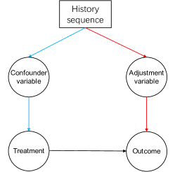
Figure 1: Causal graph of recommendation

3.2 Overview

In this work, we introduce a novel framework designed specifically to address the issue of spurious relations in sequential recommendation. This framework can be bifurcated into two integral components:

1. Adjustment Encoder $f_{\theta}$: This encoder captures the users’ genuine preferences. Techniques such as Recurrent Neural Networks or self-supervised methods (e.g., GRU, BERT) are employed to extract these true user preferences.

2. Confounder Encoder $f_{\phi}$: Parallel in structure to the adjustment encoder, the confounder encoder is tasked with extracting user representations that might lead to spurious correlations when discerning preferences from historical interactions. It is pivotal to note that the confounder encoder is exclusively employed during the training phase to negate these inadvertent correlations.

By synergizing the representations derived from both the confounder and adjustment encoders, we formulate an objective function tailored to optimize the task. Subsequent sections will delve into each of the aforementioned components in meticulous detail.

3.3 Sequential recommendation Model

The sequential recommendation model is employed within both the confounder encoder and the adjustment encoder. The sequential recommendation model comprises three parts: item embedding parts, sequence encoder layer, and next-item prediction layers.

Item Embedding Parts

Firstly, all items are embedded into the same space to produce an item embedding matrix $M\in R^{|I|\times d}$ [10], where $|I|$ denotes the item set and $d$ signifies the dimension of the embedding. Given the input history sequence $S^{u}=[c_{1},c_{2},...,c_{n}]$, the sequence’s embedding $S^{u}$ is initialized to $e^{u}\in R^{n\times d}$ where $e^{u}=[m_{s_{1}}+p_{1},m_{s_{2}}+p_{2},...,m_{s_{n}}+p_{n}]$. Here, $m_{s_{i}}\in R^{d}$ is the item’s embedding at position $k$ in the sequence, $p_{k}\in R^{d}$ is the position’s embedding, and $n$ is the sequence length.

Sequence Encoder Layer

The sequence encoder layer derives the representation of $e^{u}$ using a deep neural network (e.g., Bert4Rec) [17]. This is defined as $f_{\theta}$, where $\theta$ represents the model’s parameters. The output representation $H^{u}\in R^{n\times d}$ is calculated as:

$$H^{u}=f_{\theta}(e^{u})$$

Given our task is predicting the next item, we employ the final vector $h^{n}$ in $H^{u}=[h_{1},h_{2},...,h_{n}]$ as the representation of historical items.

Next-Item Prediction Layers

Lastly, we determine the probability of each item as $\hat{y}=h^{u}_{n}M^{T}$. In our model, the BPR loss is optimized to heighten the probability of a correct prediction given user $u$ and a pair of positive and negative items $i$ and $j$:

$$BPR_{uij}=-ln\sigma(\hat{x}_{ui}-\hat{x}_{uj})$$ (1)

Where $\sigma$ is the logistic sigmoid function:

$$\sigma(x)=\frac{1}{1+e^{-x}}$$ (2)

3.4 Spurious relation elimination part

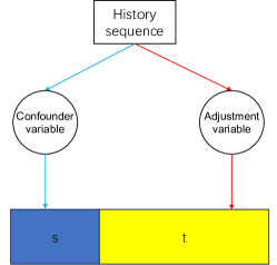
Figure 2: (a) During the training phase, the model derives a specific embedding vector from variables $x$, consisting of an adjustment component $t$ and a spurious relation component $s$. (b) In the test phase, the spurious relation component $s$ is discarded, and only the adjustment component $t$ is employed in the recommendation process.

As depicted in Fig. 2, the primary concept of our proposed framework is elaborated. In the training phase, we impose constraints on the model to yield a specialized representation vector from variables $x$. This vector encompasses two distinct components: the spurious relation component $s$, accounting for the indirect effect, and the adjustment component $t$, responsible for the direct effect. We anticipate the spurious relation component $s$ to encapsulate the entire deviations observed in the feedback label due to the spurious relation, while the adjustment component $t$ discerns the ideal feedback label portion that arises from genuine user preferences. During the test phase, the spurious relation component $s$ is disregarded, and only the adjustment component $t$ is used to enhance recommendation accuracy.

From Fig 2, we can discern that for a more precise recommendation, we must satisfy the following conditions at a minimum:

1. To avert the influence of the spurious relation, the adjustment component shouldn’t overfit to variables $x$.

2. Owing to the role of the direct effect, the adjustment component should accurately predict the label $y$.

3. The adjustment component $t$ and the spurious relation $s$ should remain as independent as possible to ensure a clear distinction, i.e., $s\perp t$.

4. Because of the indirect effect’s role, the adjustment component $t$ should also predict label $y$ to some degree.

We have deliberately not constrained the relationship between the adjustment component $t$ and the variables $x$ since the dependency level between them hinges on the feedback data’s inherent bias. Arbitrarily optimizing this might lead to undesirable outcomes. Drawing inspiration from information theory, we can formulate the required objective function based on the aforementioned analysis:

$$\mathcal{L}:=\underbrace{\beta I(t;x)}_{(1)}-\underbrace{I(t;y)}_{(2)}+\underbrace{\gamma I(t;s)}_{(3)}-\underbrace{\alpha I(s;y)}_{(4)}$$ (3)

Where:

• Term (1) is a compression term, characterizing the mutual information between variables $x$ and the adjustment embedding $t$.

• Term (2) is an accuracy term, detailing the performance of the adjustment embedding $t$.

• Term (3) acts as a de-confounder penalty term, illustrating the dependency magnitude between the spurious embedding $s$ and the adjustment embedding $t$.

• Term (4) is another accuracy term, considering the potential benefits accrued from the spurious embedding $s$.

Here, $\beta$, $\gamma$, and $\alpha$ are the respective weight parameters. By optimizing $\mathcal{L}$, we aim to obtain the desired spurious and adjustment embeddings, subsequently pruning the spurious relationship. Equation (4) stands as a vital optimization objective to steer the model towards the spurious relation embedding vector. Introducing further reasonable targets, grounded in Equation (4), could assist in securing a more precise adjustment embedding vector.

Despite the provided equation, calculating $\mathcal{L}$ remains a challenge due to its inherent complexity. We seek a more tractable solution by considering an upper bound.

Using the chain rule of mutual information, we express the deconfounder penalty term in $\mathcal{L}$ as:

$$I(t;s)=I(t;y)-I(t;y|t)+I(t;s|y)$$ (4)

Inspecting the term $I(t;s|y)$ in Equation (4), we realize that the distribution of $t$ depends solely on $x$ (which in turn is affected by $y$). This gives us:

$$H(t|y,s)=H(t|y)$$ (5)

where $H(|)$ represents the bpr loss. Using properties of mutual information, we deduce:

$$I(t;s|y)=H(t|y)-H(t|y,s)=0$$ (6)

Substituting Equation (5) into Equation (4), we get:

$$I(t;s)=I(t;y)-I(t;y|s)$$ (7)

Given the complexity of the term $I(t;y|s)$ in Equation (6), we simplify further using the concept of conditional entropy:

$$I(t;s)=I(t;y)-H(y|s)+H(y|t,s)$$ (8)

By integrating the findings from Equations (3) and (7), we can redefine $\mathcal{L}$ from Equation (3) as:

$$\mathcal{L} =\beta I(t;x)-I(t;y)+\gamma I(t;s)-\alpha I(s;y)$$ (9)

$$=\beta I(t;x)-I(t;y)+\gamma[I(t;y)-H(y\mid s)+H(y\mid t,s)]-\alpha I(s;y)$$

$$=\beta I(t;x)-(1-\gamma)I(t;y)-\gamma H(y\mid s)+\gamma H(y\mid t,s)-\alpha I(s;y)$$

We can find that only the compression term I (t;x) is related to the variables x in Equation (8). To optimize it directly, we describe a simple and precise expression of this mutual information using a method similar to that in [8, 20]. First, based on the relationship between mutual information and Kullback-Leibler (KL) divergence, the compression term I (t; x) can be calculated as follows:

$$I(t;x) =\mathbb{E}_{x}[D_{\mathrm{KL}}(p(t|x)\|p(t))]$$ (10)

$$=\sum_{x}p(x)\sum_{t}p(t|x)\log p(t|x)-\sum_{t}p(t)\log p(t)$$

However, the marginal probability $p(t)=xp(t|x)p(x)$ is usually difficult to be calculated in practice. We use variational approximation to address this issue, i.e., we use a variational distribution $q(t)$ instead of $p(t)$. According to Gibbs’ inequality, we know that the KL divergence is non-negative. Therefore, we can derive an upper bound of Equation (9),

$$\begin{array}[]{ll}&D_{\mathrm{KL}}(p(t)\|q(t))\geq 0\\ &\Rightarrow-\sum_{t}p(t)\log p(t)\leq-\sum_{t}p(t)\log q(t)\\ &\Rightarrow D_{\mathrm{KL}}(p(t\mid x)\|p(t))\leq D_{\mathrm{KL}}(p(t\mid x)\|q(t)).\end{array}$$ (11)

Similar to most previous works[14], we can assume that the posterior $p(t|x)$ is a Gaussian distribution(i.e.,$p(t|x)=N(\mu(x),diag{\sigma^{2}(x)})$),where $\mu(x)$ is the encoded embedding of the variables $x$ and $diag{\sigma 2(x)}$ is the diagonal matrix indicating the variance. Through the re-parameterization trick, the embedding $t$ can be generated according to $t=\mu(x)+\epsilon\dot{\sigma}(x)$, where $\epsilon~{}N(0,I)$. Obviously, if we fix $\sigma(x)$ to be an all-zero matrix, $t$ will reduce to a deterministic embedding. On the other hand, the prior $q(t)$ is assumed to be a standard Gaussian variational distribution, i.e., $q(t)=N(0,I)$. Finally, we can rewrite the above upper bound,

$$D_{\mathrm{KL}}(p(t\mid x)\|q(t))=\frac{1}{2}\|\mu(x)\|_{2}^{2}+\frac{1}{2}\sum_{d}\left(\sigma_{d}^{2}-\log\sigma_{d}^{2}-1\right),$$ (12)

where $\sigma_{d}^{2}$ is an element in $diag{\sigma^{2}(x)}$, i.e., $diag{\sigma^{2}(x)}={\sigma_{d}^{2}}_{d=1}^{D}$ . This means that for a deterministic embedding $t$, we can optimize this upper bound by directly applying the $l_{2}$-norm regularization on the embedding vector $t$, which is equivalent to optimizing the compression term $I(t;x)$. Note that the compression term in previous works acts on the entire biased representation $t^{*}$ , and we only compress the unbiased component $t$ of the representation.

Finally, as we have:

$$I(t;y)=H(y)-H(y|t)$$ (13)

and since $H(y)$ is a positive constant and can be ignored, we can deduce the following inequality:

$$I(t;y)\geq-H(y|t)$$ (14)

This logic also applies to the mutual information $I(s;y)$ in Equation (8).

Given these relationships, we can express the loss function, which we denote as $\mathcal{L}$, in the following manner:

$$\mathcal{L} =\beta I(t;\text{x})-(1-\gamma)I(t;y)-\gamma H(y\mid s)+\gamma H(y\mid t,s)-\alpha I(s;y)$$ (15)

$$\leq\beta\|\mu(\text{x})\|_{2}^{2}+(1-\gamma)H(y\mid t)-(\gamma-\alpha)H(y\mid s)+\gamma H(y\mid t,s).$$ (16)

Upon simplifying $\mathcal{L}$, we arrive at a more tractable solution:

$$\hat{\mathcal{L}}=\underbrace{(1-\gamma)H(y\mid t)}_{\text{(a)}}-\underbrace{(\gamma-\alpha)H(y\mid s)}_{\text{(b)}}+\underbrace{\gamma H(y\mid t,s)}_{\text{(c)}}+\underbrace{\beta\|\mu(\text{x})\|_{2}^{2}}_{\text{(d)}}$$ (17)

4 Experiment Design

4.1 Research Questions

We are seek to deal with the following questions::(RQ1)How does the proposed framework perform in real-world recommendation scenarios? (RQ2) What is the role of each term in equation (14)?

Table 1: Statistic information of experimented datasets

Datasets	#users	#items	#actions	avg.length	sparsity
Sports	33598	18357	296337	8.3	99.95%
Beauty	22363	12101	198502	8.8	99.93%

4.2 Dataset

To validate the efficiency of our approach, we tested the model on two benchmark datasets from the real-world: Amazon Beauty and Amazon Sports. These datasets are derived from user reviews on amazon.com, one of the world’s leading e-commerce platforms. Our experiments focus on two specific sub-categories: Amazon-Beauty and Amazon-Sports. Following the preprocessing steps outlined by [22], interactions involving users and items with fewer than five engagements are excluded. The characteristics of the curated datasets are detailed in Table 1.

4.3 Baseline

We compared our approach against several general sequential models:

• GRU4Rec [7] employs the Gated Recurrent Unit (GRU) for sequential recommendation.

• SASRec [10] introduced the attention mechanism to sequential recommendation, yielding notable performance.

• BERT4Rec [17] leverages deep bidirectional self-attention to discern potential relationships between items and their sequences in a Cloze task.

4.4 Metrics

To evaluate, the data is partitioned into training, validation, and testing subsets based on timestamps provided in the datasets [10]. Specifically, the last item is designated for testing, the penultimate for validation, and all preceding items for training. Following [13, 19], we rank the complete item set without employing negative sampling. To ensure comprehensive model assessment, we employ two prevalent evaluation metrics: Hit Ratio @k (HR@k) and Normalized Discounted Cumulative Gain @k (NDCG@k), where $k\in\{5,10,20\}$. While the HR metric checks if the actual result is ranked within the top k items, the NDCG metric offers a position-sensitive ranking assessment.

4.5 Implementation Details

For optimization, the Adam optimizer was employed, with hyper-parameters fine-tuned on the validation set. To ensure parity in comparisons, the batch size was fixed at 256, the embedding dimension at 64, and the maximum history length at 20 across all methodologies. The learning rate oscillated within the range $[1e-3,5e-4,1e-4]$, and weight decay was adjusted between $[1e-4,1e-6,1e-8,0]$. Additional hyper-parameters specific to the baselines were tuned within ranges recommended by their respective authors. The performance of the three base models refers from [16]. For transparency and replicability, the source codes have been made publicly accessible.

5 Experiment Result

5.1 RQ1

We evaluated the efficacy of our model, Irl4Rec, against prominent models, including GRU4Rec, SASRec, and BERT4Rec. For consistent and unbiased assessment, all models underwent identical preprocessing and were evaluated using two metrics: NDCG@k and Hit Ratio@k (HR@k), with $k\in[5,10,20]$. The results, delineated in Table 2, yield several insightful observations:Irl4Rec outperforms the other three models, solidifying its superior capabilities in the given context. Our proposed structure exhibits enhanced performance particularly with BERT4Rec. This can be attributed to the BERT encoder’s prowess in gleaning pertinent information from historical data. When juxtaposing the improvements in BERT4Rec and GRU4Rec, it’s evident that for the beauty dataset, the enhancements in BERT4Rec surpassed those in GRU4Rec. Conversely, for the sports dataset, our Irl4Rec displayed a more significant boost when paired with GRU4Rec. Overall, the standout performance of Irl4Rec can be traced back to its adeptness at discerning and leveraging spurious relationships inherent in the datasets. "In our evaluation of the SASRec model, we found evidence of our proposed models’ efficiency across different datasets. While there was a decline in the NDCG@10 metric for the sports dataset, the overall experimental results still indicate that our models are efficient.

Table 2: Performance comparisons of proposed model and base model(sport)

Model	HR@5	HR@10	HR@20	NDCG@5	NDCG@10	NDCG@20
GRU4Rec	0.0126	0.0203	0.0316	0.0082	0.0106	0.0135
GRU4Rec+	0.0164	0.0250	0.0394	0.0107	0.0135	0.0171
improvement(%)	30.16	23.15	25.08	30.49	27.36	26.67
BERT4Rec	0.0217	0.0359	0.0604	0.0143	0.0190	0.0251
BERT4Rec+	0.0260	0.0385	0.0566	0.0172	0.0213	0.0258
improvement(%)	19.81	7.24	-6.29	20.27	10.94	2.79
SASRec	0.0214	0.0333	0.0500	0.0144	0.0177	0.0224
SASRec+	0.0248	0.0369	0.0549	0.0207	0.0168	0.0252
improvement(%)	15.89	10.81	9.8	43.75	-5.08	12.5

Table 3: Performance comparisons of proposed model and base model(beauty)

Model	HR@5	HR@10	HR@20	NDCG@5	NDCG@10	NDCG@20
GRU4Rec	0.0168	0.0289	0.0461	0.0103	0.0142	0.0185
GRU4Rec+	0.0203	0.0334	0.0559	0.0119	0.0164	0.0218
improvement(%)	20.83	15.57	21.26	15.53	15.49	17.84
BERT4Rec	0.0360	0.0601	0.0984	0.0216	0.0300	0.0391
BERT4Rec+	0.0458	0.0661	0.0935	0.0302	0.0367	0.0435
improvement(%)	27.22	9.98	-4.97	39.81	22.33	11.25
SASRec	0.0377	0.0624	0.0894	0.0241	0.0342	0.0386
SASRec+	0.0441	0.0656	0.0937	0.0299	0.0368	0.0439
improvement(%)	30.86	5.12	4.81	24.06	7.60	1373

5.2 RQ2(Ablation Study)

In our ablation study, we adopted NDCG@20 and HR@20 as evaluation metrics and centered our experiments on the BERT4Rec model, given its recent prominence and frequent application in sequential recommendation tasks. The results reveal several key observations: For the beauty dataset, our model consistently surpasses other approaches in all three segments of the ablation study, marking a new state-of-the-art benchmark. In contrast, with the sports dataset, term (2) doesn’t significantly impact the predictions. This discrepancy could be attributed to the sports dataset’s larger volume when compared to the beauty dataset, thereby heightening the likelihood of overfitting. Omitting term (1) leads to a discernible decline in performance, emphasizing its integral role. This outcome aligns with expectations since term (1) functions as the training objective for adjustment variables, which are pivotal in the recommendation schema. In summation, every constituent of our proposed framework collectively converges to realize the maximal performance gains.

Table 4: Ablation study(on Bert4Rec)

	sport		beauty
BERT4Rec+	HR@20	NDCG@20	HR@20	NDCG@20
raw	0.0550	0.0252	0.0937	0.0439
w/o (1)	0.0436	0.0184	0.0776	0.0344
w/o (2)	0.0553	0.0256	0.0935	0.0435
w/o (3)	0.0550	0.0246	0.0908	0.0413

6 CONCLUSION AND FUTURE WORK

In this study, we present an innovative approach to Top-k sequential recommendation with a particular focus on addressing the challenge posed by spurious relations. To this end, we introduce a causal graph methodology and unveil the Irl4Rec model. Irl4Rec is rooted in the principles of invariant learning. It not only emphasizes the intricate relationship between spurious relation variables and adjustment variables but also proposes a novel objective to address the issue at hand. Our experiments, conducted on Amazon’s sport and beauty datasets, attest to Irl4Rec’s prowess in enhancing the efficacy of existing methods. This marked improvement can be primarily attributed to the adept integration of invariant learning coupled with our novel objective.

However, Irl4Rec is not without its limitations. Its integration with contrastive learning — a leading technique in sequential recommendation — remains a challenge. As we chart our future research direction, our ambition is to devise strategies that effectively handle spurious relations in sequential history items, all the while harnessing the power of contrastive learning during training. Ultimately, we aspire to refine Irl4Rec such that it seamlessly integrates with a broader spectrum of sophisticated models.

6.0.1 Acknowledgements

Please place your acknowledgments at the end of the paper, preceded by an unnumbered run-in heading (i.e. 3rd-level heading).

References

- [1] K. Ahuja, E. Caballero, D. Zhang, J.-C. Gagnon-Audet, Y. Bengio, I. Mitliagkas, and I. Rish. Invariance principle meets information bottleneck for out-of-distribution generalization, 2022.
- [2] K. Ahuja, K. Shanmugam, K. R. Varshney, and A. Dhurandhar. Invariant risk minimization games, 2020.
- [3] M. Arjovsky, L. Bottou, I. Gulrajani, and D. Lopez-Paz. Invariant risk minimization, 2020.
- [4] P. Bühlmann. Invariance, causality and robustness. 2020.
- [5] S. Feng, X. Li, Y. Zeng, G. Cong, and Y. M. Chee. Personalized ranking metric embedding for next new poi recommendation. In IJCAI’15 Proceedings of the 24th International Conference on Artificial Intelligence, pages 2069–2075. ACM, 2015.
- [6] F. Garcin, C. Dimitrakakis, and B. Faltings. Personalized news recommendation with context trees. In Proceedings of the 7th ACM Conference on Recommender Systems, pages 105–112, 2013.
- [7] B. Hidasi and A. Karatzoglou. Recurrent neural networks with top-k gains for session-based recommendations. In Proceedings of the 27th ACM international conference on information and knowledge management, pages 843–852, 2018.
- [8] A. Jaiswal, R. Brekelmans, D. Moyer, G. V. Steeg, W. AbdAlmageed, and P. Natarajan. Discovery and separation of features for invariant representation learning, 2019.
- [9] W.-C. Kang and J. McAuley. Self-attentive sequential recommendation. In 2018 IEEE international conference on data mining (ICDM), pages 197–206. IEEE, 2018.
- [10] W.-C. Kang and J. McAuley. Self-attentive sequential recommendation, 2018.
- [11] K. Khezeli, A. Blaas, F. Soboczenski, N. Chia, and J. Kalantari. On invariance penalties for risk minimization, 2021.
- [12] M. Koyama and S. Yamaguchi. When is invariance useful in an out-of-distribution generalization problem ?, 2021.
- [13] W. Krichene and S. Rendle. On sampled metrics for item recommendation. In Proceedings of the 26th ACM SIGKDD international conference on knowledge discovery & data mining, pages 1748–1757, 2020.
- [14] D. Liang, R. G. Krishnan, M. D. Hoffman, and T. Jebara. Variational autoencoders for collaborative filtering, 2018.
- [15] J. Liu, Z. Hu, P. Cui, B. Li, and Z. Shen. Heterogeneous risk minimization. In International Conference on Machine Learning, pages 6804–6814. PMLR, 2021.
- [16] X. Qin, H. Yuan, P. Zhao, J. Fang, F. Zhuang, G. Liu, Y. Liu, and V. Sheng. Meta-optimized contrastive learning for sequential recommendation. In Proceedings of the 46th International ACM SIGIR Conference on Research and Development in Information Retrieval. ACM, jul 2023.
- [17] F. Sun, J. Liu, J. Wu, C. Pei, X. Lin, W. Ou, and P. Jiang. Bert4rec: Sequential recommendation with bidirectional encoder representations from transformer. In Proceedings of the 28th ACM international conference on information and knowledge management, pages 1441–1450, 2019.
- [18] S. Wang, L. Hu, Y. Wang, L. Cao, Q. Z. Sheng, and M. Orgun. Sequential recommender systems: challenges, progress and prospects. arXiv preprint arXiv:2001.04830, 2019.
- [19] X. Wang, X. He, M. Wang, F. Feng, and T.-S. Chua. Neural graph collaborative filtering. In Proceedings of the 42nd International ACM SIGIR Conference on Research and Development in Information Retrieval. ACM, jul 2019.
- [20] Z. Wang, X. Chen, R. Wen, S.-L. Huang, E. E. Kuruoglu, and Y. Zheng. Information theoretic counterfactual learning from missing-not-at-random feedback, 2020.
- [21] G.-E. Yap, X.-L. Li, and P. S. Yu. Effective next-items recommendation via personalized sequential pattern mining. In Database Systems for Advanced Applications: 17th International Conference, DASFAA 2012, Busan, South Korea, April 15-19, 2012, Proceedings, Part II 17, pages 48–64. Springer, 2012.
- [22] K. Zhou, H. Wang, W. X. Zhao, Y. Zhu, S. Wang, F. Zhang, Z. Wang, and J.-R. Wen. S3-rec: Self-supervised learning for sequential recommendation with mutual information maximization. In Proceedings of the 29th ACM international conference on information & knowledge management, pages 1893–1902, 2020.