Black holes in degenerate Einstein Gauss-Bonnet gravity: Can QNMs distinguish them from GR?

Abstract

In this study, for the first time, we analyse the quasinormal modes of black holes occurring within the framework of degenerate gravity. We investigate the properties of the asymptotically flat spacetimes introduced recently in [JCAP $02(2022)02$] that satisfy degenerate Einstein Gauss-Bonnet(dEGB) action and belong to a much larger class of solutions which include cosmological constant. This solution has two distinct branches akin to Einstein Gauss-Bonnet(EBG) gravity. However, unlike the EBG solutions, both the branches of dEGB are well-defined asymptotically. The negative branches from both theories can be identified for the asymptotically flat case. We observe black holes for specific ranges of the Gauss-Bonnet coupling parameter and perform a stability analysis by calculating the quasinormal modes (QNMs) under scalar wave propagation. Finally, the ringdown spectrums of our black holes are compared with their GR counterparts.

I Introduction

Over the years, there has been significant interest in formulating a gravitational framework incorporating Gauss-Bonnet(GB) and higher-order Lovelock densities in four and higher dimensions[1, 2, 3, 4, 5, 6, 7, 8, 9]. However, these higher-order Lovelock densities within four dimensions do not affect the dynamics of the gravity. Mathematically, these terms do not contribute to the Euler-Lagrange equations of motion [10, 11, 12]. Any attempts to introduce these higher-order terms must confront the issues of additional degrees of freedom or involving derivatives higher than second order.

However, recently Glavan and Lin [13] demonstrated that it is possible to construct a theory of gravity that satisfies the conditions mentioned earlier while still exhibiting a dynamic influence of Gauss-Bonnet density. This is achieved by introducing a “singular-rescaling” of GB coupling and then taking a $D\rightarrow 4$ limit of a $D\geq 5$ action. Thus these solutions are interpreted as four-dimensional with non-trivial imprints of the GB coupling. However, it was later realised that this formulation is neither covariant nor the limit is well defined [14, 15, 16, 17, 18, 19, 20, 21, 22, 23, 24]. Upon close inspection, it was further revealed that these solutions could be realised in various other frameworks of gravity [25, 26, 16, 27, 28, 29].

In the context of first-order formulation, a similar dynamical imprint of GB density has been achieved in [30]. Unlike the earlier approaches, this framework does not rely on singular rescaling nor introduces any new dynamical fields. Instead, this is achieved using the notion of “extra dimensions of zero proper length” introduced in [31]. A similar analysis has been implemented to obtain a dynamical theory of gravity in two dimensions[32]. This new theory is more general than the Jackiw-Teitelboim gravity[33, *jackiw1t] and inequivalent to the Mann-Ross prescription[35, *mann1t1, *mann1t2]. In general, metric solutions with zero determinant have been investigated as a potential resolution to curvature singularities and dark matter problems, which are serious challenges to General Relativity. Similarly, a degenerate extension to the Reissner-Nordström metric has been explored in [38, 39], which resolves the problem of curvature singularity and provides a natural geometric interpretation of electric and magnetic charges.

In this current work, we explore the ringdown aspects of the black hole solutions within the dEGB theory, highlighting the difference from their GR counterpart. We begin by addressing the issue of stability of these new solutions under the propagation of a massless scalar field and compute the QNMs. The QNMs are compared with that of the GR vacuum black hole solutions to understand the dependence of the QNMs on the underlying gravity theory. Apart from that, it is well known that the solutions in higher-dimensional Einstein-Gauss-Bonnet theory in the metric formulation are plagued with instability occurring at higher multipole numbers[40, 41, 42, 43, 44, 45, 46, 47, 48, 49]. One wonders if these solutions to degenerate EGB theory are also plagued with similar issues. Hence, this study becomes particularly pertinent as the initial step in probing any possible instabilities of the solutions in this unique dEGB theory.

Lately, quasinormal modes of various compact objects have been the focus of research in multiple works in literature where they are being used as a tool to distinguish different geometries, and also to identify black hole mimicking nature of various compact objects [50, 51, 52, 53, 54, 55, 56]. Such studies are especially relevant in the era of gravitational wave detections as QNMs play a crucial role in commenting on the stability of spacetime, the estimation of parameters of the remnant and also determining the underlying theory of gravity [57, 58, 59]. On the other hand, in the context of GW data analysis, computing QNMs in alternative theories of gravity [60, 61, 62, 49, 63, 64, 65, 66] is crucial for formulating ringdown tests of GR [67, 68, 69, 70, 71, 72]. These tests help constrain the possible GR violations by estimating the difference of QNMs between GR and the other theories of gravity using the ringdown signal of a binary merger event. Some works have also shown the possible detection of multi-mode ringdown signals to be a unique test of the black hole nature of the remnant formed from coalescence [73, 74]. The future generation detectors with their enhanced sensitivity will be an ideal ground for implementing these tests, highlighting the relevance of our study [75, 76, 77]. Therefore, comparing the observational signatures, like ringdown behaviour and QNMs of the black hole solutions in our degenerate EGB theory with that of GR is highly relevant in the era of gravitational wave detections which will be dealt with in our paper.

The structure of our work is as follows. In Section II, we provide a concise description of the gravity theory under consideration, along with an introduction to the spherically symmetric, static solution that is the focus of our study. Section III discusses the classification of the spacetimes and their properties. Sections IV delves into the computation of QNMs under propagation of scalar wave for all the black holes belonging to our dEGB theory. We conclude this paper with a summary of the results obtained and a brief perspective on the future extensions of this work in the final Section V. The main results of our work is summarized in the form of two tables; Table 1 discusses the classification of spacetimes and Table 6 shows the dependence of QNMs on ($\kappa,Q^{2}$).

II Revisiting the Degenerate EGB theory

We begin by summarizing the main results of [30], which formulates the framework of degenerate EGB gravity. Understanding this theory of gravity itself is crucial before analyzing the properties and stability of its static, spherically symmetric solutions. We begin with the action for the degenerate EGB gravity of the form

$$\mathcal{L}(\hat{e},\hat{\omega})=\epsilon^{\mu\nu\alpha\beta\gamma}\epsilon_{IJKLM}\left[\frac{\alpha}{2}\hat{R}_{\mu\nu}^{IJ}(\hat{\omega})\hat{R}_{\alpha\beta}^{KL}(\hat{\omega})\hat{e}_{\gamma}^{M}+\frac{\zeta}{2}\hat{R}_{\mu\nu}^{IJ}(\hat{\omega})\hat{e}^{K}_{\alpha}\hat{e}^{L}_{\beta}\hat{e}_{\gamma}^{M}+\frac{\beta}{5}\hat{e}^{I}_{\mu}\hat{e}^{J}_{\nu}\hat{e}^{K}_{\alpha}\hat{e}^{L}_{\beta}\hat{e}^{M}_{\gamma}\right]$$ (1)

where the independent fields are the vielbein $\hat{e}^{I}_{\mu}$ and $\hat{\omega}^{IJ}_{\mu}(\mu\equiv\left[t,x,y,z,\upsilon\right],I\equiv\left[0,1,2,3,4\right])$ are the super-connection. The parameters $\alpha,\zeta,\beta$ correspond to the Gauss-Bonnet coupling, gravitational coupling, and the bare cosmological constant, respectively. Varying the action with respect to these independent fields lead to the following equations of motion

$$\begin{split}&\epsilon^{\mu\nu\alpha\beta\gamma}\epsilon_{IJKLM}\left[\alpha\hat{R}_{\mu\nu}^{IJ}(\hat{\omega})+\zeta\hat{e}^{I}_{\mu}\hat{e}_{\nu}^{J}\right]\hat{D}_{\alpha}(\hat{\omega})\hat{e}_{\beta}^{K}=0\\ &\epsilon^{\mu\nu\alpha\beta\gamma}\epsilon_{IJKLM}\left[\frac{\alpha}{2}\hat{R}_{\mu\nu}^{IJ}(\hat{\omega})\hat{R}_{\alpha\beta}^{KL}(\hat{\omega})+\zeta\hat{R}_{\mu\nu}^{IJ}(\hat{\omega})\hat{e}^{K}_{\alpha}\hat{e}^{L}_{\beta}+\beta\hat{e}^{I}_{\mu}\hat{e}^{J}_{\nu}\hat{e}^{K}_{\alpha}\hat{e}^{L}_{\beta}\right]=0\end{split}$$ (2)

where $\hat{D}_{\alpha}(\hat{\omega})$ represents the gauge-covariant derivative with respect to the super-connections $\hat{\omega}_{\mu}^{IJ}$. The Bianchi identity $\hat{D}_{\left[\mu\right.}\hat{R}_{\left.\nu\alpha\right]}^{IJ}(\hat{\omega})=0$ is also utilized to simplify the equations of motions and obtain them in the form stated above (eq.(2)).

Now we restrict our analysis to the vielbeins whose determinant is zero. For this case, without the loss of generality, we can assume an ansatz such that the zero eigenvalue of the vielbein $\hat{e}^{I}_{\mu}$ lies along the fifth direction $(\upsilon)$ which can be written as

$$\begin{split}\hat{e}^{I}_{\upsilon}&=0\\ \hat{e}^{I}_{\mu}&=\begin{bmatrix}\hat{e}^{i}_{a}\equiv e^{i}_{a}&0\\ 0&0\end{bmatrix}\end{split}$$ (3)

where we have used the notation of $\mu\equiv(a,\upsilon)\equiv(t,x,y,z,\upsilon)$ and $I\equiv(i,4)\equiv(0,1,2,3,4)$. Certain conclusions can be made by using the ansatz (3) in equations of motion (2) which are listed below.

• An effective four-dimensional spacetime can be defined using the tetrads $e^{i}_{a}$, which are invertible, unlike the five vielbein.

• The emergent four-dimensional spin connections satisfy the zero torsion condition.

• All emergent four-dimensional fields are independent of the fifth dimension, and any such dependence is a gauge artefact.

• Finally, the only remaining unsolved component of the field equations is

  $$\epsilon^{abcd}\epsilon_{ijkl}\left[\phi\beta\bar{R}_{ab}^{ij}e^{k}_{c}e^{l}_{d}+\frac{\alpha}{2}\bar{R}_{ab}^{ij}\bar{R}_{cd}^{kl}+\xi e^{i}_{a}e^{j}_{b}e^{k}_{c}e^{l}_{d}\right]=0$$ (4)

where $\bar{R}^{ij}_{ab}$ is the four dimensional torsion-free field strength tensor. Further details and analysis of these results can be found in [30].

Static, spherically symmetric solutions

In order to obtain a static, spherically symmetric solution to the field equation (4), we consider the ansatz

$$ds^{2}=-e^{\mu(r)}dt^{2}+\frac{dr^{2}}{e^{\mu(r)}}+r^{2}d\Omega^{2}$$ (5)

which can be substituted into eq.(4) to obtain the functional form of $e^{\mu(r)}$

$$e^{\mu}=1+\frac{\phi}{2\alpha}r^{2}\pm\frac{1}{2}\left[\left(\frac{\phi^{2}}{\alpha^{2}}-\frac{2\chi}{\alpha}\right)r^{4}+4C_{1}r-\frac{4C_{2}}{\alpha}\right]^{\frac{1}{2}}$$ (6)

where $\alpha$ is the Gauss-Bonnet coupling and $\phi$,$\chi$ are the theory’s parameters, and $C_{1}$ and $C_{2}$ are the constants of integration. The above metric component asymptotically reduces to the form

$$e^{\mu}\rightarrow 1-\frac{\Lambda_{eff}}{3}\pm\left(\frac{2M_{eff}}{r}-\frac{Q_{eff}^{2}}{r^{2}}\right)$$ (7)

where we have identified the effective mass, charge and cosmological constant in terms of our metric parameters as

$$\Lambda_{eff}=\frac{-3}{2}\left(\frac{\phi}{\alpha}\pm\sqrt{\frac{\phi^{2}}{\alpha^{2}}-\frac{2\chi}{\alpha}}\right)$$ (8)

$$2M_{eff}=\frac{C_{1}}{\sqrt{\frac{\phi^{2}}{\alpha^{2}}-\frac{2\chi}{\alpha}}}$$ (9)

$$Q^{2}_{eff}=\frac{C_{2}}{\alpha\sqrt{\frac{\phi^{2}}{\alpha^{2}}-\frac{2\chi}{\alpha}}}$$ (10)

Imposing the conditions that effective mass is positive and the charge is real implies $C_{1}<0(C_{1}>0)$ and $C_{2}<0(C_{2}>0)$ for the $+(-)$ branches respectively. We would also like to emphasise that $Q_{eff}$ of our theory is inequivalent to the charge originating from Maxwell Electrodynamics, as is evident from the absence of any matter fields in our action. $Q_{eff}$ is geometric in origin and in a spirit similar to what has been explored in [78, 79]. Similar constructions of electric and magnetic charges in degenerate spacetimes have been explored in [38, 39] where the origin of such charges was demonstrated to be associated with topological invariants. The exact origin of $Q_{eff}$ in the dEGB theory discussed in our work still remains to be understood. We will drop the subscript eff from the effective ‘asymptotic’ parameters $\Lambda_{eff},Q_{eff},M_{eff}$ for brevity for the rest of the paper.

In the next section, we will focus on the possible asymptotically flat spacetimes permitted in the dEGB theory and discuss their properties.

III Classification of solutions: with and without geometric charge

III.1 Solution without geometric charge: Positive branch

Let us start our analysis by examining the positive branch of the solutions (eq.(6)) given by

$$e^{\mu}=1+\frac{\phi}{2\alpha}r^{2}+\frac{1}{2}\left[\left(\frac{\phi^{2}}{\alpha^{2}}-\frac{2\chi}{\alpha}\right)r^{4}+4C_{1}r-\frac{4C_{2}}{\alpha}\right]^{\frac{1}{2}}$$ (12)

The absence of geometric charge and asymptotic flatness would mean

$$C_{2}=0$$

$$\Lambda=0\implies\frac{\chi}{\alpha}=0;\quad\frac{\phi}{\alpha}<0$$

$$C_{1}=-2M\Big{|}\frac{\phi}{\alpha}\Big{|}$$

implementing which the metric for the positive branch can be recast as

$$e^{\mu}=1-\frac{r^{2}}{2\kappa}\left(1-\left(1-\frac{8M\kappa}{r^{3}}\right)^{\frac{1}{2}}\right)$$ (13)

with the redefinition $|\frac{\alpha}{\phi}|=\kappa>0$. This is the form of the metric which will be used in subsequent calculations in this section.

From eq.(13), it is evident that the radial coordinate is constrained to the range $(8M\kappa)^{\frac{1}{3}}<r<\infty$, beyond which the metric component becomes imaginary. The strictly greater limit imposed is justified by looking at the exact expression of the Ricci scalar

$$R=\frac{-120\kappa^{2}M^{2}+\kappa Mr^{3}\left(72-48\sqrt{1-\frac{8\kappa M}{r^{3}}}\right)+r^{6}\left(6\sqrt{1-\frac{8\kappa M}{r^{3}}}-6\right)}{\kappa r^{3}\left(r^{3}-8\kappa M\right)\sqrt{1-\frac{8\kappa M}{r^{3}}}}$$ (14)

which shows that there is a curvature singularity at $r=r_{min}=(8M\kappa)^{\frac{1}{3}}$. To determine the position of the horizon or the infinite redshift surface for the above metric we solve,

$$e^{\mu}=0\implies-\frac{r^{2}}{2k}\left(1-\frac{8M\kappa}{r^{3}}\right)^{\frac{1}{2}}=1-\frac{r^{2}}{2\kappa}$$ (15)

Squaring both sides of eq.(15) reduces it to a quadratic polynomial equation of the form

$$r^{2}-2Mr-\kappa=0$$ (16)

having solutions

$$r_{\pm}=M\pm\sqrt{M^{2}+\kappa}$$ (17)

Only the $r_{+}$ is admissible of the two roots as $r_{-}$ leads to negative radial values for $\kappa>0$. However, note that the above solutions correspond to the squared equation, which may or may not satisfy the original equation in eq.(15).

Let us further analyse the eq.(15) at the horizon $r=r_{h}$

$$-\frac{r_{h}^{2}}{2k}\left(1-\frac{8M\kappa}{r_{h}^{3}}\right)^{\frac{1}{2}}=1-\frac{r_{h}^{2}}{2\kappa}$$ (18)

Since $\kappa>0$ and the square root term gives only a positive value, the LHS is always negative. Hence the above equation is only satisfied if

$$1-\frac{r_{h}^{2}}{2\kappa}=\frac{\kappa-2M^{2}-2M\sqrt{M^{2}+\kappa}}{2\kappa}\leq 0$$ (19)

with $r_{h}$ expressed in terms of $\kappa$ and giving

$$\kappa-2M^{2}-2M\sqrt{M^{2}+\kappa}\leq 0$$ (20)

The above inequality is satisfied for $\kappa\leq 8M^{2}$, where the equality is achived at $\kappa=8M^{2}$. Beyond this range of $\kappa$ the inequality is violated and there are no horizons. Note that for $\kappa=8M^{2}$, the event horizon coincides with the curvature singularity, forming a naked singularity. We will focus on cases with $\kappa<8M^{2}$ to only study the black hole solutions.

III.2 Solution without geometric charge: Negative branch

We now focus on the solution which has the negative sign in eq.(6) corresponding to the negative branch having the form

$$e^{\mu}=1+\frac{\phi}{2\alpha}r^{2}-\frac{1}{2}\left[\left(\frac{\phi^{2}}{\alpha^{2}}-\frac{2\chi}{\alpha}\right)r^{4}+4C_{1}r-\frac{4C_{2}}{\alpha}\right]^{\frac{1}{2}}$$ (21)

As with the previous case, we impose the conditions of asymptotic flatness and zero geometric charge which for the negative branch are given by

$$C_{2}= \,0$$

$$\Lambda= 0\implies\frac{\chi}{\alpha}=0;\quad\frac{\phi}{\alpha}>0$$

$$C_{1}= \,2M\frac{\phi}{\alpha}$$

Implementing the above conditions along with the parameter $\kappa=\frac{\alpha}{\phi}>0$ in the negative branch, the metric function becomes

$$e^{\mu}=1+\frac{r^{2}}{2\kappa}\left(1-\left(1+\frac{8M\kappa}{r^{3}}\right)^{\frac{1}{2}}\right)$$ (22)

We will use the above form of the metric function for the rest of the calculations in this section. Note that this solution matches the metric explored in [13], with the identification of $\kappa$ to the GB coupling in [13]. However, the range of $\kappa$ does not match the range of GB coupling in [13] due to the conditions on the constraints being unrelated. We believe this correspondence is coincidental, as these solutions do not match in presence of a cosmological constant. For completeness, we proceed with our analysis of the metric properties and in the later sections will explore their corresponding QNMs.

The Ricci scalar for this case has a form

$$R=\frac{120\kappa^{2}M^{2}+\kappa Mr^{3}\left(72-48\sqrt{\frac{8\kappa M}{r^{3}}+1}\right)+r^{6}\left(6-6\sqrt{\frac{8\kappa M}{r^{3}}+1}\right)}{\kappa r^{3}\left(8\kappa M+r^{3}\right)\sqrt{\frac{8\kappa M}{r^{3}}+1}}$$ (23)

which, unlike the positive branch, is singular only at $r=0$. Hence the range of radial coordinate is unobstructed, and $r$ takes the values from $0<r<\infty$. After finding the position of singularity, we move on to check the presence of horizons by solving

$$e^{\mu}=0\implies 1+\frac{r^{2}}{2\kappa}=\frac{r^{2}}{2\kappa}\left(1+\frac{8M\kappa}{r^{3}}\right)^{\frac{1}{2}}$$ (24)

Squaring both sides gives the horizon at

$$r_{\pm}=M\pm\sqrt{M^{2}-\kappa}$$ (25)

Since $\sqrt{M^{2}-\kappa}<M$, we have two horizons corresponding to the two solutions. $\kappa=M^{2}$ results in an extremal case where both the horizons merge, producing a black hole solution with a single horizon. Hence for the negative branch, the allowed range of parameter $\kappa$ is $0<\kappa\leq M^{2}$. Note that unlike the positive branch for the range $r>0$, the LHS and RHS of (24) are always positive; hence all the values of $\kappa$ in the range $0<\kappa\leq M^{2}$ are valid solutions.

III.3 Charged static spherically symmetric solution: Positive branch

We will now deal with the solutions having a non-zero geometric charge $Q$. Starting with the positive branch, we have the metric of the form

$$e^{\mu}=1+\frac{\phi}{2\alpha}r^{2}+\frac{1}{2}\left[\left(\frac{\phi^{2}}{\alpha^{2}}-\frac{2\chi}{\alpha}\right)r^{4}+4C_{1}r-\frac{4C_{2}}{\alpha}\right]^{\frac{1}{2}}$$ (26)

Similar to the cases without geometric charge, we impose the asymptotic flatness giving rise to conditions

$$\Lambda=0\implies\frac{\chi}{\alpha}=0;\quad\frac{\phi}{\alpha}<0$$

$$\frac{C_{2}}{\alpha}=-Q^{2}|\frac{\phi}{\alpha}\Big{|}$$

$$C_{1}=-2M\Big{|}\frac{\phi}{\alpha}\Big{|}$$

which are used to recast the metric as,

$$e^{\mu}=1-\frac{r^{2}}{2\kappa}\left(1-\left(1-\frac{8M\kappa}{r^{3}}+\frac{4Q^{2}\kappa}{r^{4}}\right)^{\frac{1}{2}}\right)$$ (27)

with $|\frac{\alpha}{\phi}|=\kappa>0$. This is the metric form that will be used in subsequent calculations involving the positive branch with non-zero $Q$.

The Ricci scalar for the above metric can be written as

$$R=\frac{F(r,M,Q,\kappa)}{\kappa r^{8}\left(\frac{-8\kappa Mr+4\kappa Q^{2}+r^{4}}{r^{4}}\right)^{3/2}}$$ (28)

where the exact form of $F(r,M,Q)$ is not relevant for us since we focus only on the position of curvature singularity given by the roots of $r^{4}-8\kappa Mr+4\kappa Q^{2}=0$. This quartic equation has to be solved numerically for each value of $(\kappa,M,Q)$ giving the position of curvature singularity and hence the allowed range of the radial coordinate.

Similar to the previous cases, the position of the horizon is determined by solving

$$e^{\mu}=0\implies-\frac{r^{2}}{2k}\left(1-\frac{8M\kappa}{r^{3}}+\frac{4Q^{2}\kappa}{r^{4}}\right)^{\frac{1}{2}}=1-\frac{r^{2}}{2\kappa}$$ (29)

which on squaring reduces to a quadratic equation

$$r^{2}-2Mr-\kappa+Q^{2}=0$$ (30)

having solutions

$$r_{\pm}=M\pm\sqrt{M^{2}-Q^{2}+\kappa}$$ (31)

Depending on the value of $\kappa$ and $Q^{2}$, the metric can have one or two positive roots and hence horizons, but in the context of QNMs (which is the focus of the current work), we are only interested in the outer horizon located at $r=r_{+}$. Note that if we demand the presence of a horizon in spacetime, we get a constraint on the geometric charge

$$Q^{2}\leq M^{2}+\kappa$$ (32)

Following the analysis done in the case without geometric charge, we determine if all the solutions given in eq.(31) actually satisfy the horizon condition of eq.(29).

At the horizon $r=r_{h}$, eq.(29) becomes

$$-\frac{r_{h}^{2}}{2k}\left(1-\frac{8M\kappa}{r_{h}^{3}}+\frac{4\kappa Q^{2}}{r^{4}}\right)^{\frac{1}{2}}=1-\frac{r_{h}^{2}}{2\kappa}$$ (33)

The LHS of the above equation is always negative since $\kappa>0$ and the term under square root gives only a positive value. Hence the equation is satisfied only if

$$1-\frac{r_{h}^{2}}{2\kappa}=\frac{\kappa-2M^{2}+Q^{2}-2M\sqrt{M^{2}-Q^{2}+\kappa}}{2\kappa}\leq 0$$ (34)

with $r_{h}$ expressed in terms of $\kappa$, leading to the condition

$$\kappa-2M^{2}+Q^{2}-2M\sqrt{M^{2}-Q^{2}+\kappa}\leq 0$$ (35)

The above inequality is satisfied for $0<\kappa\leq\frac{1}{2}M^{2}$ provided the charge is constrained as suggested in eq.(32). However, for $\kappa\geq\frac{1}{2}M^{2}$, we get additional condition on charge given by

$$Q^{2}\leq 2\sqrt{2\kappa M^{2}}-\kappa\leq M^{2}+\kappa$$ (36)

In Fig.1, we show the allowed range of metric parameters in the parameter space of $(Q^{2},\kappa)$. The shaded region corresponds to black hole solutions while the parameter values falling on the dotted line give naked singularity. The yellow shaded region denotes black holes with $Q^{2}/M^{2}\geq 1$ where the equality corresponds to the extremal case. Note that $Q$ beyond the extremal value is allowed in this degenerate theory of gravity.

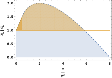
Figure 1: Shaded region represents allowed parameter range of $\kappa$ and $Q^{2}$ for black hole solutions. The yellow region depicts extreme charge to mass ratios, while the parameters on the dotted lines lead to naked singularities.

III.4 Charged static spherically symmetric solution: Negative Branch

Once again, we analyse the negative branch of the solution in the presence of a non-zero geometric charge having the metric

$$e^{\mu}=1+\frac{\phi}{2\alpha}r^{2}-\frac{1}{2}\left[\left(\frac{\phi^{2}}{\alpha^{2}}-\frac{2\chi}{\alpha}\right)r^{4}+4C_{1}r-\frac{4C_{2}}{\alpha}\right]^{\frac{1}{2}}$$ (37)

To ensure asymptotic flatness of the spacetime, the following conditions must be imposed on the parameters

$$\Lambda=0\implies\frac{\chi}{\alpha}=0;\quad\frac{\phi}{\alpha}>0$$ (38)

$$\frac{C_{2}}{\alpha}=Q^{2}\frac{\phi}{\alpha}$$ (39)

$$C_{1}=2M\frac{\phi}{\alpha}$$ (40)

giving the metric as

$$e^{\mu}=1+\frac{r^{2}}{2\kappa}\left(1-\left(1+\frac{8M\kappa}{r^{3}}-\frac{4Q^{2}\kappa}{r^{4}}\right)^{\frac{1}{2}}\right)$$ (41)

with $\frac{\alpha}{\phi}=\kappa>0$. The Ricci scalar for this case is given by

$$R=\frac{F(r,M,Q,\kappa)}{\kappa r^{8}\left(\frac{8\kappa Mr-4\kappa Q^{2}+r^{4}}{r^{4}}\right)^{3/2}}$$ (42)

where, similar to the positive branch case, we do not concern with the exact form of $F(r,M,Q)$. We calculate the roots of $r^{4}+8\kappa Mr-4\kappa Q^{2}=0$ numerically and find the position of curvature singularity which gives the allowed range of radial coordinate for specific choice of $(\kappa,Q^{2})$. To find the horizon, we solve

$$e^{\mu}=0\implies\frac{r^{2}}{2k}\left(1+\frac{8M\kappa}{r^{3}}-\frac{4Q^{2}\kappa}{r^{4}}\right)^{\frac{1}{2}}=1+\frac{r^{2}}{2\kappa}$$ (43)

which on squaring reduces to a quadratic equation

$$r^{2}-2Mr+\kappa+Q^{2}=0$$ (44)

with solution

$$r_{\pm}=M\pm\sqrt{M^{2}-Q^{2}-\kappa}$$ (45)

Depending the value of $(\kappa,Q^{2})$, the metric can have one or two positive roots and hence horizons, but we will focus only on the outer horizon $r_{+}$ since we will deal with QNMs of the spacetime. We also obtain the following constraint on the geometric charge,

$$Q^{2}\leq M^{2}-\kappa$$ (46)

which ensures presence of horizon in the spacetime. To check whether $r_{\pm}$ of eq.(45) are indeed the solutions to transcendental equations of eq.(43), we evaluate them at the horizon $r=r_{h}$

$$\frac{r_{h}^{2}}{2k}\left(1+\frac{8M\kappa}{r_{h}^{3}}-\frac{4\kappa Q^{2}}{r^{4}}\right)^{\frac{1}{2}}=1+\frac{r_{h}^{2}}{2\kappa}$$ (47)

Since $\kappa>0$ and the square root term gives only a positive value, the LHS is always positive. Hence the above equation is only satisfied if

$$1-\frac{r_{h}^{2}}{2\kappa}=\frac{2M^{2}-Q^{2}+2M\sqrt{M^{2}-Q^{2}-\kappa}}{2\kappa}\geq 0$$ (48)

where we have expressed $r_{h}$ in terms of $\kappa$ which reduces to

$$2M^{2}-Q^{2}+2M\sqrt{M^{2}-Q^{2}-\kappa}\geq 0$$ (49)

The above inequality is automatically satisfied for the range $0<\kappa\leq M^{2}$ and $Q^{2}\leq M^{2}-\kappa$, hence any value $\kappa$ and $Q$ within the parameter range is allowed.

Table 1 summarizes the properties and parameter ranges for the black hole solutions discussed in this section corresponding to positive and negative branch. In the next segment of this paper we will compute the ringdown spectrum and quasinormal modes of these black holes under scalar wave propagation.

	Branch	Metric	Horizon	Allowed parameters
Q = 0	$+$	$e^{\mu}=1-\frac{r^{2}}{2\kappa}\left(1-\left(1-\frac{8M\kappa}{r^{3}}\right)^{\frac{1}{2}}\right)$	$r_{\pm}=M\pm\sqrt{M^{2}+\kappa}$	$0\leq\kappa\leq 8M^{2}$
	$-$	$e^{\mu}=1+\frac{r^{2}}{2\kappa}\left(1-\left(1+\frac{8M\kappa}{r^{3}}\right)^{\frac{1}{2}}\right)$	$r_{\pm}=M\pm\sqrt{M^{2}-\kappa}$	$0<\kappa\leq M^{2}$
Q $\neq$ 0	$+$	$e^{\mu}=1-\frac{r^{2}}{2\kappa}\left(1-\left(1-\frac{8M\kappa}{r^{3}}+\frac{4Q^{2}\kappa}{r^{4}}\right)^{\frac{1}{2}}\right)$	$r_{\pm}=M\pm\sqrt{M^{2}-Q^{2}+\kappa}$	$Q^{2}\leq 2\sqrt{2\kappa M^{2}}-\kappa,\quad 0<\kappa\leq\frac{M^{2}}{2}$ $Q^{2}\leq M^{2}+\kappa,\quad\frac{M^{2}}{2}<\kappa<8M^{2}$
	$-$	$e^{\mu}=1+\frac{r^{2}}{2\kappa}\left(1-\left(1+\frac{8M\kappa}{r^{3}}-\frac{4Q^{2}\kappa}{r^{4}}\right)^{\frac{1}{2}}\right)$	$r_{\pm}=M\pm\sqrt{M^{2}-Q^{2}-\kappa}$	$0<\kappa\leq M^{2}$, $Q^{2}\leq M^{2}-\kappa$

Table 1: Table shows asymptotically flat black hole solutions in the dEGB theory, their horizon position, and allowed parameter ranges.

IV Stability analysis: Scalar wave propagation and quasinormal modes

We will now probe the stability of the black hole spacetimes studied in the previous section by computing their corresponding QNMs and ringdown behaviour under the propagation of the scalar wave. For astrophysical objects in our universe, it is natural to expect their stability under various perturbations. Gravitational perturbations are the most stringent check of stability for any spacetime. However, in the context of the degenerate framework of gravity, the perturbations of the tetrad fields are not well understood and require dedicated attention, which is beyond the scope of this paper. Hence we resort to the simplest probe of stability i.e. the propagation of a massless test scalar field. This would be considered the first step towards exploring the stability of these new spacetimes.

We begin with the Klein-Gordon equation for a massless scalar field

$$\Box\Phi=0$$ (50)

It is important to note that the scalar field $\Phi$ serves as a test field and does not directly affect the metric. However, the propagation scalar field is influenced by the background geometry. As our background spacetime is spherically symmetric and static, we decompose $\Phi$ in terms of spherical harmonics, where the indices of $Y(\theta,\phi)$ have been suppressed for simplicity

$$\Phi(t,r,\theta,\phi)=Y(\theta,\phi)\frac{u(r)e^{-i\omega t}}{r}$$ (51)

Incorporating this ansatz in eq.(50), we obtain the radial equation of the form of a Schrödinger-like equation by using the tortoise coordinate $r_{*}\left(dr_{*}=\frac{dr}{e^{\mu}}\right)$,

$$\frac{d^{2}u}{dr_{*}^{2}}+[\omega^{2}-V_{eff}]u=0$$ (52)

where the effective potential is

$$V_{eff}(r)=e^{\mu}\Big{(}\frac{\ell(\ell+1)}{r^{2}}+\frac{\left(e^{\mu}\right)^{\prime}}{r}\Big{)}$$ (53)

Furthermore, $\ell$ is the azimuthal number arising from the separation of variables. In the forthcoming sections, we will plot the effective potential for specific solutions and parameter values and comment on their nature. To compute the discrete quasinormal modes, we implement the well-studied semi-analytical WKB technique along with Padé improvements [80, 81, 82]. In order to visualize the behaviour of the scalar field ($\Phi(t,r,\theta,\phi)=Y(\theta,\phi)\psi(r,t)$), we plot its evolution in time. We recast the equation for $\psi(r,t)$,

$$\frac{\partial^{2}\psi}{\partial t^{2}}-\frac{\partial^{2}\psi}{\partial r_{*}^{2}}+V_{eff}(r_{*})\psi=0.$$ (54)

using light cone coordinates $(u,v)$ such that $(du=dt-dr_{*},dv=dt+dr_{*})$. The detailed discretization scheme is discussed in [83, 56]. An initial Gaussian pulse is evolved over the null grid which is dominated by the QNMs of the corresponding spacetime, dampening of which would indicate its stability. The QNMs computed with the WKB method have been verified through the Prony extraction technique [83, 56, 55], although not quoted in the paper, as implementing the Prony extraction for all cases considered is time consuming.

IV.1 QNMs of positive branch solution without geometric charge

We begin the stability analysis by plotting the effective potential obtained in eq.(53) as a function of the radial coordinate $r$ for various values of $\kappa$ belonging to the positive branch case shown in Fig.(2). In our QNM analysis, we will consider $M=1$ unless otherwise stated.

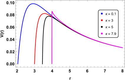
Figure 2: Plot showing variation of V(r) with the radial coordinate for $\ell=1$ and different values of $\kappa$ for positive branch and zero geometric charge.

It is evident that all values of $\kappa<8$ have single barrier potential and hence the WKB method can be applied to obtain the QNMs.

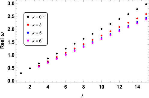
Figure 3: Plot showing variation real part of the fundamental QNM for different values of $\ell$ and $\kappa$ for positive branch and zero geometric charge.

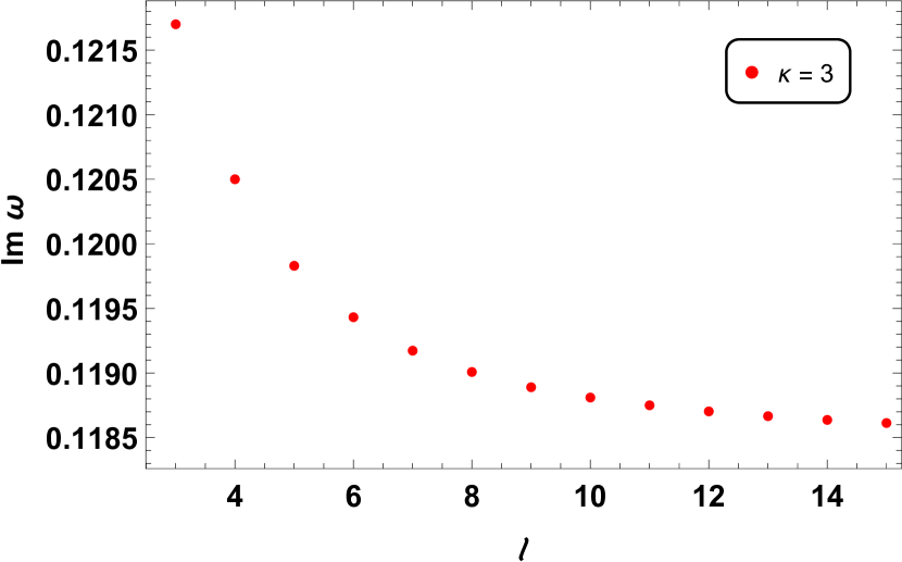
Figure 4: Plots showing the variation of the imaginary part of the fundamental QNM for $\kappa=0.1,3$ as a function of $\ell$ for positive branch and zero geometric charge.

Fig.(3) and (4) show the dependence of the real and imaginary part of QNM on the metric parameter $\kappa$ leading to the following observations:

• We observe from Fig.(3), as the angular momentum mode increases, the real component of the quasinormal modes (QNMs) show a corresponding increase, indicating a rise in frequency. Although distinct, the magnitudes of the modes are very close for different values of $\kappa$ especially for small $\ell$. Also, the WKB method is suitable for higher values of $\ell$. Hence we have not computed the QNMs for $\kappa=3,5,6$ corresponding to very low $\ell$ values as the different orders of the WKB method fail to converge.

• The imaginary component, on the other hand, decreases with $\ell$ for all values of $\kappa$. This indicates that the higher modes have longer damping time and can dominate the signal at later stages.

• Comparing the fundamental modes for different values of $\kappa$, we observe that the frequency and damping time decreases as $\kappa$ increases. This is evident from the corresponding time domain profiles for different $\kappa$ as shown in the Fig:(5) where the time domain signal for $\kappa=6$ decays much faster than smaller $\kappa$ geometries.

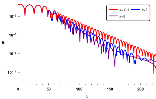
Figure 5: Ringdown profile for different $\kappa$ in the positive branch case with $Q=0$ as observed at $r_{*}=6,\ell=3$ with initial Gaussian profile $\psi=e^{\frac{-(u-6)^{2}}{100}}$ and grid spacing of 0.5.

For a vanishing coupling constant, the theory reduces to GR with the only vacuum, static, spherically symmetric solution being the Schwarzschild case. We thus compare the scalar QNMs generated by a Schwarzschild black hole with that of our solution with a small coupling constant. This analysis will help us visualize the difficulty of segregating the two kinds of solutions only through their scalar QNMs and highlight the QNMs’ dependence on the underlying gravity theory. Table 2 shows that the fundamental QNMs for small $\kappa$ are significantly close (upto the accuracy considered here) to the corresponding QNMs of Schwarzschild black hole for a particular angular momentum mode. Hence, in actual observation, a highly sensitive detector will be required to distinguish the solution of our theory with a small $\kappa$ from a Schwarzschild black hole.

$\ell$	Schwarzschild	$\kappa=0.001$	$\kappa=0.01$	$\kappa=0.1$
1	0.292909 -i 0.09776	0.292928 -i 0.097405	0.292692 -i 0.097818	0.290542 -i 0.099187
2	0.48364 -i 0.096757	0.483610 -i 0.096733	0.483274 -i 0.096908	0.480022 -i 0.0982177
3	0.675365 -i 0.096499	0.675436 -i 0.098474	0.674859 -i 0.096646	0.670409 -i 0.097922

Table 2: Comparison of fundamental $\omega_{QNM}$ for different $\kappa$ values corresponding to the positive branch of $Q=0$ case with that of the Schwarzschild black hole.

IV.2 QNMs of negative branch solution without geometric charge

Similar to the positive branch solution, we will compute the scalar quasinormal modes associated with the negative branch solution by solving eq.(52). Fig.(6) shows the effective potential being a single barrier for different values of $\kappa$. Thus the WKB method with Padé improvements can be applied to compute the fundamental QNMs.

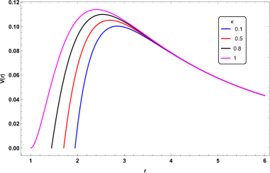
Figure 6: Plot showing variation of V(r) with the radial coordinate for $\ell=1$ and various values of $\kappa$ corresponding to negative branch solution with zero geometric charge.

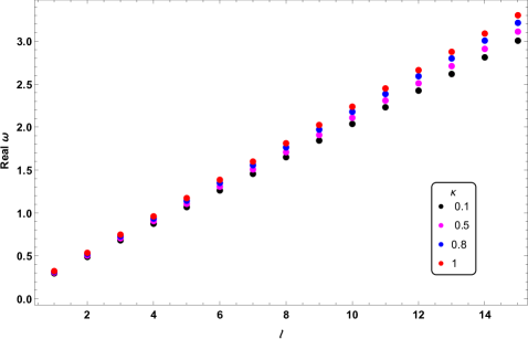
Figure 7: Plot showing the variation of the real part of the fundamental QNM with $\ell$ for various values of $\kappa$ corresponding to negative branch solution with $Q=0$.

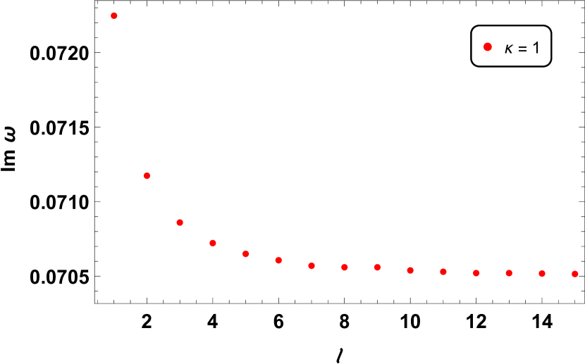
Figure 8: Plots showing the variation of the imaginary part of the fundamental QNM for $\kappa=0.1,1$ with $\ell$ corresponding to negative branch solution with $Q=0$.

The variation of real and imaginary components of the QNMs with the angular momentum mode for different $\kappa$ are shown in Figs.(7) and (8). In contrast to the positive branch case, the real component of the fundamental mode increases with increasing $\kappa$. The imaginary part, on the other hand, decreases as $\kappa$ increases, evident from their time domain profiles as shown in Fig(9).

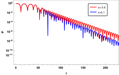
Figure 9: Ringdown profile for different $\kappa$ corresponding to negative branch solution with $Q=0$ as observed at $r_{*}=6,\ell=3$ with initial Gaussian profile $\psi=e^{\frac{-(u-6)^{2}}{100}}$ and grid spacing 0.5.

As done for the positive branch, we compute the QNMs for different $\kappa$ values and compare them with the Schwarzschild case. Table 3 shows that small $\kappa$ solutions indeed have almost identical QNMs to that of the Schwarzschild black hole. The distinction becomes more prominent as $\kappa$ increases.

$\ell$	Schwarzschild	$\kappa=0.001$	$\kappa=0.1$	$\kappa=0.7$	$\kappa=0.9$
1	0.292909 -i 0.09776	0.2931761 -i 0.0975015	0.295398 -i 0.096027	0.3122758 -i 0.083077	0.318868 -i 0.076427
2	0.48364 -i 0.096757	0.484015 -i 0.096608	0.487438 -i 0.0952057	0.51529 -i 0.082522	0.527432 -i 0.075695
3	0.675365 -i 0.096499	0.6758755 -i 0.096352	0.680578 -i 0.094978	0.719381 -i 0.082369	0.736788 -i 0.075478

Table 3: Comparison of fundamental $\omega_{QNM}$ for different $\kappa$ values belonging to the negative branch with zero geometric charge with that of the Schwarzschild black hole.

IV.3 QNMs of positive branch solution with geometric charge

Before we begin the discussion of the QNMs, we study the plots for some of the potentials corresponding to various values of charge and Gauss-Bonnet coupling as shown in Fig.(10). We find the effective potentials to be single barrier for all $(\kappa,Q)$ hence QNM frequencies can be computed via WKB technique.

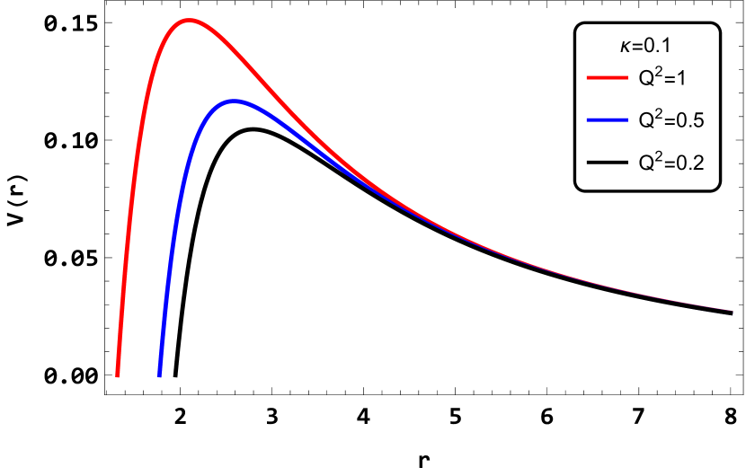
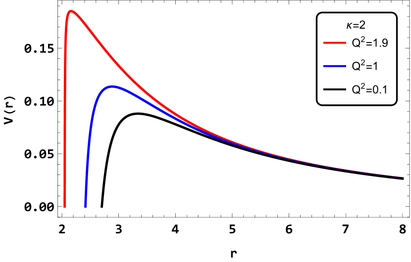
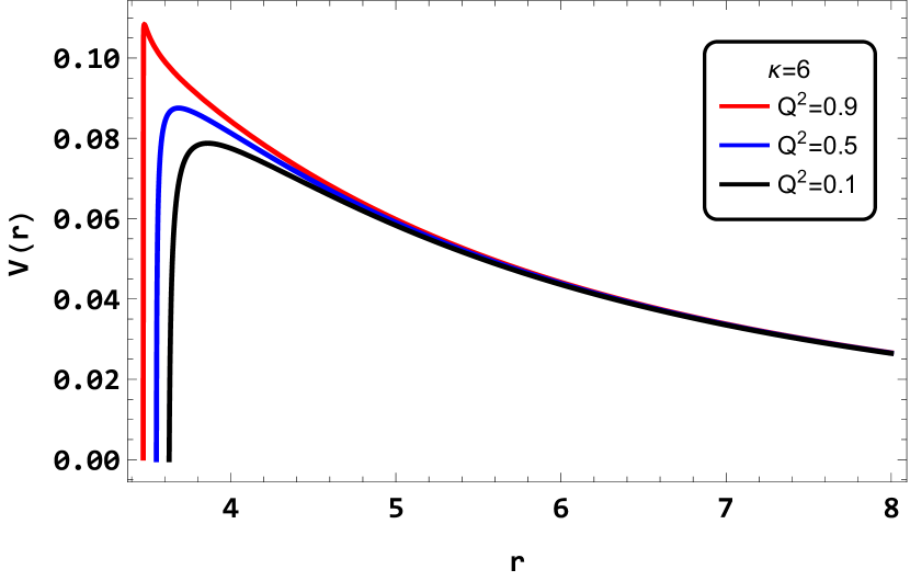
Figure 10: Potential plots of the positive branch solutions for various values of $\kappa$ and $Q$, where $\ell=1$.

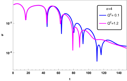
Figure 11: Ringdown profile for $\kappa=4$ and different $Q^{2}$ corresponding to positive branch solution as observed at $r_{*}=6,\ell=1$ with initial Gaussian profile $\psi=e^{\frac{-(u-6)^{2}}{100}}$ and grid spacing 0.5.

Since the QNMs now depend on both $Q$ and $\kappa$, we plot the QNMs for a fixed $\ell$ and study the dependence of the fundamental modes on the metric parameters. Certain observations can be concluded about the QNMs for the positive branch solutions.

• It is known that the WKB techniques are suitable for larger values of $\ell$ and may not provide convergent results for lower values. However, the stability of the system can be established via time-domain profiles which was done in this case for small $\ell$. As an example, we demonstrate the damping of the signal over time, indicating the stability of spacetime for $\kappa=4,\ell=1$ in Fig.(11). Note that the choice of $\kappa$ and $Q$ to demonstrate this is arbitrary, and the objective result regarding the stability for this branch is independent of the choice of parameters in the allowed range, i.e the spacetimes are stable for the lower value of $\ell$ for the complete range of allowed parameters.

• For higher values of $\ell$, WKB method is implemented to obtain fundamental QNMs. From the plots of Fig.(12), we observe a decrease in QNM frequency as $\kappa$ increases. The QNMs are calculated corresponding to a fixed $\kappa$ for various values of $Q$ constrained by eq.(32). For a fixed $\kappa$, the frequency increases as the charge increases. The plot is done with $\ell=10$, but similar results can also be obtained for other values of angular momentum as well.

• However, the imaginary component associated with the damping time shows some interesting properties as shown in Fig.(13). For the small value of $\kappa$, the plot of imaginary $\omega$ vs $Q^{2}$ has the same characteristic behaviour as the Reissner-Nordström black hole where Im($\omega$) increases, reaches a peak and then decreases with $Q^{2}$. Thus for one particular $\kappa$, the shortest damping time will correspond to specific $Q^{2}$ lying in the middle of the allowed charge range. However, this changes for higher values of $\kappa$ for which the imaginary component increases with an increase in charge, indicating faster signal damping for large $Q^{2}$.

(a) Small $\kappa$ solutions

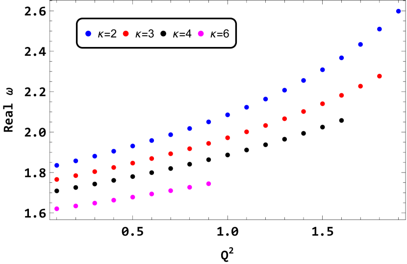
(b) Large $\kappa$ solutions

Figure 12: Plots show variation of real part of fundamental QNM with $\ell=10$ for different ($\kappa,Q$) corresponding to the positive branch solutions.

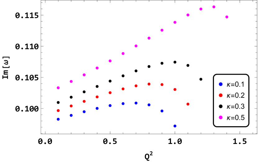
(a) Small $\kappa$ solutions

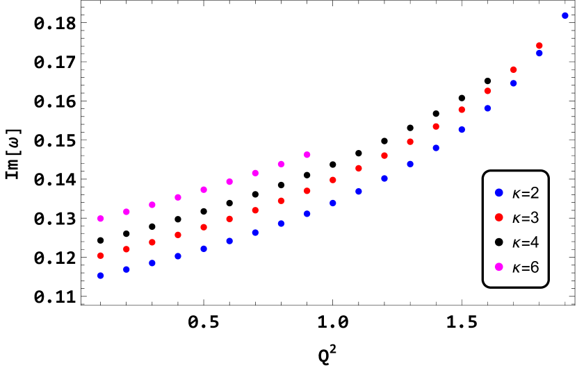
(b) Large $\kappa$ solutions

Figure 13: Plots show variation of real part of fundamental QNM with $\ell=10$ for different ($\kappa,Q$) corresponding to the positive branch solutions.

Similar to the case of zero geometric charge, we now compare the QNMs of the black holes belonging to this branch for different values of $\kappa$ with that of the Reissner-Nordström black hole as shown for the fundamental QNMs in Table 4. As expected, smaller $\kappa$ corresponding to a weaker coupling term gives QNM values closer to the R-N case.

$\ell$	Q	Reissner-Nordström	$\kappa=0.01$	$\kappa=0.1$
1	0.1	0.293407  -0.0978114 i	0.293168  -0.0979535 i	0.291007  -0.0992218 i
	0.9	0.352625  -0.0972076 i	0.352036  -0.0972604 i	0.347043  -0.101713 i
2	0.1	0.484455  -0.0968185 i	0.484082  -0.0969688 i	0.480797  -0.0982871 i
	0.9	0.581952  -0.0966326 i	0.580974  -0.0971101 i	0.572645  -0.100969 i
3	0.1	0.676499  -0.0965534 i	0.675988  -0.096701 i	0.671501  -0.0979877 i
	0.9	0.812568  -0.0964701 i	0.811185  -0.0969426 i	0.799493  -0.100743 i

Table 4: Comparison of fundamental $\omega_{QNM}$ for different values of $\kappa$ and $Q$ with that of the Reissner-Nordström black hole.

IV.4 QNMs of negative branch solution with geometric charge

As with the other previous solutions, we move on to discuss the potentials for various values of $Q$ and Gauss-Bonnet coupling and compute the corresponding QNMs under the propagation of the scalar field. The plots of Fig.(14) show the effective potential for different ($\kappa,Q$) as a function of radial coordinate. Once again, the potential is found to be a single barrier for all parameter values, and hence the WKB method can be applied to compute the QNMs.

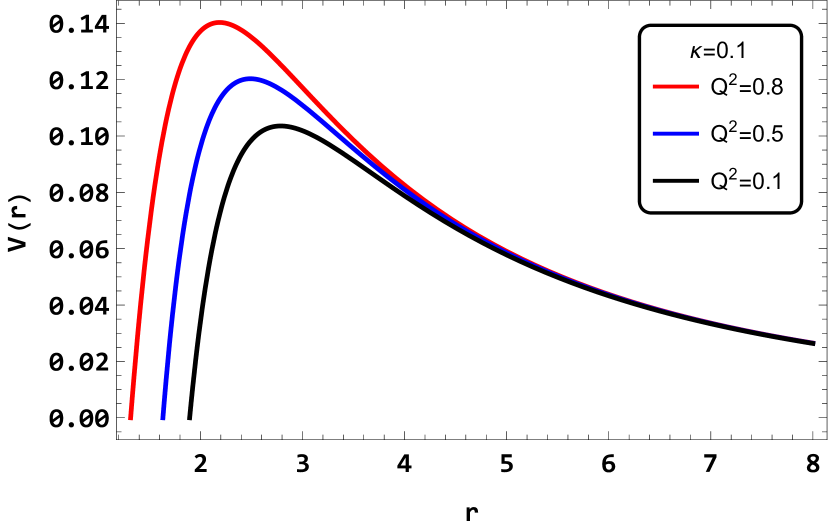
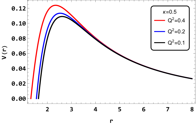
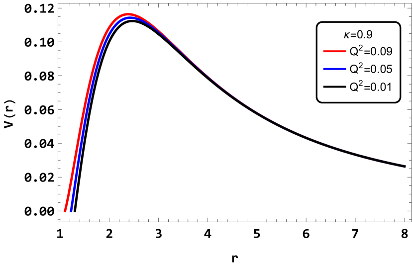
Figure 14: Potential plots for various values of $\kappa$ and $Q$ with $\ell=1$ for negative branch solutions.

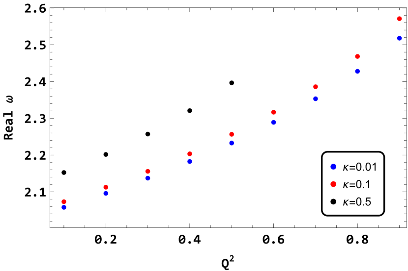
(a) Variation of real part of $\omega$

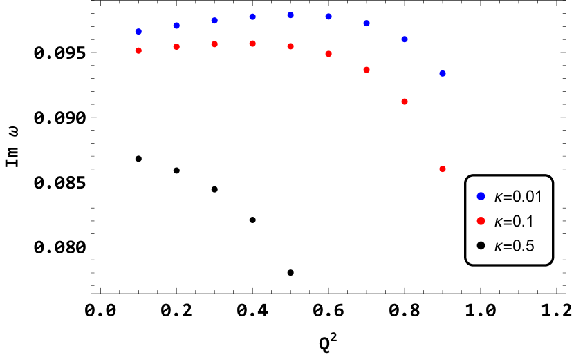
(b) Variation of imaginary part of $\omega$

Figure 15: Plots showing variation of real and imaginary components of $\omega_{QNM}$ for different ($\kappa,Q^{2}$) with $\ell=10$.

In Fig.(15), we show the dependence of real and imaginary components of QNM on ($\kappa,Q^{2}$) for $\ell=10$. We observe that for a particular $\kappa$, as $Q^{2}$ increases, the frequency increases and so does the damping time. Finally, we comment on the similarity of fundamental modes for small $\kappa$ solutions with the Reissner-Nordström metric as shown in Table 5. We observe that indeed the negative branch black holes for small $\kappa$ have QNMs very close to the R-N black hole and would require high precision observation to distinguish between them.

$\ell$	Q	Reissner-Nordström	$\kappa=0.01$	$\kappa=0.1$
1	0.1	0.293407  -0.0978114 i	0.293645  -0.0976688 i	0.295797  -0.0963567 i
	0.9	0.352625  -0.0972076 i	0.35319  -0.0967101 i	0.358452  -0.0914129 i
2	0.1	0.484455  -0.0968185 i	0.484829  -0.0966674 i	0.488285  -0.0952389 i
	0.9	0.581952  -0.0966326 i	0.582942  -0.0961435 i	0.592422  -0.0910936 i
3	0.1	0.676499  -0.0965534 i	0.677012  -0.0964049 i	0.681755  -0.0950176 i
	0.9	0.812568  -0.0964701 i	0.81397  -0.0959856 i	0.827516  -0.0909645 i

Table 5: Comparison of fundamental $\omega_{QNM}$ for different values of $\kappa$ and $Q$ with that of the Reissner-Nordström black hole.

Table 6 summarizes the dependence of the QNMs on the metric parameters for different spacetimes discussed in this section.

Branch	$\kappa$	$Q^{2}$	Re ($\omega$)	Im ($\omega$)
$+$	Increasing	0	$\downarrow$	$\uparrow$
$-$	Increasing	0	$\uparrow$	$\downarrow$
$+$	Small	Increasing	$\uparrow$	$\uparrow$ to $\downarrow$
$+$	Large	Increasing	$\uparrow$	$\uparrow$
$-$	Fixed	Increasing	$\uparrow$	$\downarrow$

Table 6: Table shows the QNMs’ dependence on the metric parameters for different spacetimes. $\uparrow$ and $\downarrow$ indicate respectively increasing and decreasing behaviour of the corresponding quantity with the change in the parameter. The inferences are for a fixed $\ell$.

V Conclusion

In this work, we studied the asymptotically flat spacetimes that arise in the degenerate gravity framework developed in [30]. We perform a first of its kind stability analysis of solutions in degenerate gravity. This involves the computation of QNMs under scalar wave propagation of the black hole solutions in dEGB theory. We begin by analysing the metric to obtain constraints on the parameters which lead to black hole solutions. This is achieved by demanding the presence of a horizon. We also compute the Ricci scalar and demand any curvature singularity to be present behind the horizon, thus avoiding naked singularities. Spacetimes can be broadly classified into four categories depending on branch and geometric charge. For the positive branch with zero geometric charge, the Gauss-Bonnet coupling is constrained as $0<\kappa<8M^{2}$. Also note that for this case, the Ricci scalar diverges at $r=\sqrt[3]{8M\kappa}$. A similar analysis for the negative branch without geometric charge results in $0<\kappa<M^{2}$. However, unlike the positive branch, the Ricci scalar diverges only at $r=0$. Next, we explore both these branches with non-zero geometric charge. A similar analysis leads to the conclusion that the range of the geometric charge is restricted by the GB coupling in both branches. These restrictions and the parameter ranges have been discussed in detail. However, unlike the zero $Q$ case, the exact location of singularities could not be solved analytically and have been computed numerically for choices of ($\kappa,Q$) which leads to black hole solutions.

We have also probed the stability of these solutions under the propagation of the massless scalar field and have found them to be stable. The effective potentials for all cases are single barriers, making the implementation of the WKB technique for QNM computation possible. We would also like to emphasise that the convergence of WKB depends on the angular momentum mode. The spacetimes for which the WKB method was not convergent for lower values of $\ell$ the time domain profiles were computed to establish their stability. From our analysis of QNMs, we observe that the modes of our black holes converge towards their GR counterparts as GB coupling tends to zero. However, for a definite answer about the stability of these solutions, we need to check their behaviour and QNMs under gravitational perturbations, which would be a natural extension of the current work. One also wonders if these geometric charges can mimic the actual Maxwell electromagnetic charge. At least the preliminary analysis via scalar QNMs does not rule out this possibility. However, a definitive answer requires further investigations.

As for future perspectives, one can extend this analysis by adding the cosmological constant, which poses additional complexities. Alternatively, one might try to construct rotating or slow-rotating examples around these solutions and compute the shadows, QNM and other observable quantities. These results will be relevant from the gravitational waves and shadow observation standpoint. However, this is a non-trivial endeavour and will be addressed in future.

VI Acknowledgements

The authors are grateful to Sayan Kar and K.G.Arun for their valuable comments on the manuscript. S.G acknowledges the support of SERB project grant CRG/2020/002035. S.G also acknowledges the discussion and inputs of Kinjal Banerjee. P.D.R. acknowledges the support of a grant from the Infosys foundation.

References

- Boulware and Deser [1985] D. G. Boulware and S. Deser, Phys. Rev. Lett. 55, 2656 (1985).
- Castillo-Felisola et al. [2016] O. Castillo-Felisola, C. Corral, S. del Pino, and F. Ramírez, Phys. Rev. D 94, 124020 (2016), arXiv:1609.09045 [gr-qc] .
- Deruelle and Farina-Busto [1990] N. Deruelle and L. Farina-Busto, Phys. Rev. D 41, 3696 (1990).
- Klein [1926] O. Klein, Z. Phys. 37, 895 (1926).
- Madore [1985] J. Madore, Phys. Lett. A 110, 289 (1985).
- Mueller-Hoissen [1985] F. Mueller-Hoissen, Phys. Lett. B 163, 106 (1985).
- Mueller-Hoissen [1986] F. Mueller-Hoissen, Class. Quant. Grav. 3, 665 (1986).
- Wheeler [1986a] J. T. Wheeler, Nucl. Phys. B 268, 737 (1986a).
- Wheeler [1986b] J. T. Wheeler, Nucl. Phys. B 273, 732 (1986b).
- Lovelock [1971] D. Lovelock, J. Math. Phys. 12, 498 (1971).
- Lovelock [1972] D. Lovelock, J. Math. Phys. 13, 874 (1972).
- Lanczos [1938] C. Lanczos, Annals Math. 39, 842 (1938).
- Glavan and Lin [2020] D. Glavan and C. Lin, Phys. Rev. Lett. 124, 081301 (2020), arXiv:1905.03601 [gr-qc] .
- Gurses et al. [2020] M. Gurses, T. c. Şişman, and B. Tekin, Phys. Rev. Lett. 125, 149001 (2020), arXiv:2009.13508 [gr-qc] .
- Gürses et al. [2020] M. Gürses, T. c. Şişman, and B. Tekin, Eur. Phys. J. C 80, 647 (2020), arXiv:2004.03390 [gr-qc] .
- Hennigar et al. [2020] R. A. Hennigar, D. Kubizňák, R. B. Mann, and C. Pollack, JHEP 07, 027, arXiv:2004.09472 [gr-qc] .
- Shu [2020] F.-W. Shu, Phys. Lett. B 811, 135907 (2020), arXiv:2004.09339 [gr-qc] .
- Ai [2020] W.-Y. Ai, Commun. Theor. Phys. 72, 095402 (2020), arXiv:2004.02858 [gr-qc] .
- Arrechea et al. [2021] J. Arrechea, A. Delhom, and A. Jiménez-Cano, Chin. Phys. C 45, 013107 (2021), arXiv:2004.12998 [gr-qc] .
- Arrechea et al. [2020] J. Arrechea, A. Delhom, and A. Jiménez-Cano, Phys. Rev. Lett. 125, 149002 (2020), arXiv:2009.10715 [gr-qc] .
- Bonifacio et al. [2020] J. Bonifacio, K. Hinterbichler, and L. A. Johnson, Phys. Rev. D 102, 024029 (2020).
- Mahapatra [2020] S. Mahapatra, Eur. Phys. J. C 80, 992 (2020), arXiv:2004.09214 [gr-qc] .
- Hohmann et al. [2021] M. Hohmann, C. Pfeifer, and N. Voicu, Eur. Phys. J. Plus 136, 180 (2021), arXiv:2009.05459 [gr-qc] .
- Cao and Wu [2022] L.-M. Cao and L.-B. Wu, Eur. Phys. J. C 82, 124 (2022), arXiv:2103.09612 [gr-qc] .
- Lu and Pang [2020] H. Lu and Y. Pang, Phys. Lett. B 809, 135717 (2020), arXiv:2003.11552 [gr-qc] .
- Kobayashi [2020] T. Kobayashi, JCAP 07, 013, arXiv:2003.12771 [gr-qc] .
- Fernandes et al. [2020] P. G. S. Fernandes, P. Carrilho, T. Clifton, and D. J. Mulryne, Phys. Rev. D 102, 024025 (2020), arXiv:2004.08362 [gr-qc] .
- Fernandes [2021] P. G. S. Fernandes, Phys. Rev. D 103, 104065 (2021), arXiv:2105.04687 [gr-qc] .
- Aoki et al. [2020] K. Aoki, M. A. Gorji, and S. Mukohyama, Phys. Lett. B 810, 135843 (2020), arXiv:2005.03859 [gr-qc] .
- Sengupta [2022] S. Sengupta, JCAP 02 (02), 020, arXiv:2109.10388 [gr-qc] .
- Sengupta [2020] S. Sengupta, Phys. Rev. D 101, 104040 (2020), arXiv:1908.04830 [gr-qc] .
- Gera and Sengupta [2021a] S. Gera and S. Sengupta, Phys. Rev. D 104, 124050 (2021a), arXiv:2110.06252 [gr-qc] .
- Teitelboim [1984] C. Teitelboim, in QUANTUM THEORY OF GRAVITY. ESSAYS IN HONOR OF THE 60TH BIRTHDAY OF BRYCE S. DEWITT, edited by S. M. Christensen (1984) pp. 324–344.
- Cangemi and Jackiw [1992] D. Cangemi and R. Jackiw, Phys. Rev. Lett. 69, 233 (1992).
- Mann and Ross [1993] R. B. Mann and S. F. Ross, Class. Quant. Grav. 10, 1405 (1993), arXiv:gr-qc/9208004 .
- Mann et al. [1990] R. Mann, A. Shiekh, and L. Tarasov, Nuclear Physics B 341, 134 (1990).
- Sikkema and Mann [1991] A. E. Sikkema and R. B. Mann, Classical and Quantum Gravity 8, 219 (1991).
- Gera and Sengupta [2021b] S. Gera and S. Sengupta, Phys. Rev. D 104, 044057 (2021b), arXiv:2101.05964 [gr-qc] .
- Gera and Sengupta [2021c] S. Gera and S. Sengupta, Phys. Rev. D 104, 044038 (2021c), arXiv:2004.13083 [gr-qc] .
- Dotti and Gleiser [2005] G. Dotti and R. J. Gleiser, Phys. Rev. D 72, 044018 (2005), arXiv:gr-qc/0503117 .
- Gleiser and Dotti [2005] R. J. Gleiser and G. Dotti, Phys. Rev. D 72, 124002 (2005), arXiv:gr-qc/0510069 .
- Konoplya and Zhidenko [2017a] R. A. Konoplya and A. Zhidenko, JCAP 05, 050, arXiv:1705.01656 [hep-th] .
- Konoplya and Zhidenko [2017b] R. A. Konoplya and A. Zhidenko, JHEP 09, 139, arXiv:1705.07732 [hep-th] .
- Takahashi and Soda [2010] T. Takahashi and J. Soda, Prog. Theor. Phys. 124, 911 (2010), arXiv:1008.1385 [gr-qc] .
- Yoshida and Soda [2016] D. Yoshida and J. Soda, Phys. Rev. D 93, 044024 (2016), arXiv:1512.05865 [gr-qc] .
- Takahashi [2011] T. Takahashi, Prog. Theor. Phys. 125, 1289 (2011), arXiv:1102.1785 [gr-qc] .
- Konoplya and Zhidenko [2008] R. A. Konoplya and A. Zhidenko, Phys. Rev. D 77, 104004 (2008), arXiv:0802.0267 [hep-th] .
- Takahashi [2013] T. Takahashi, PTEP 2013, 013E02 (2013), arXiv:1209.2867 [gr-qc] .
- Blázquez-Salcedo et al. [2017] J. L. Blázquez-Salcedo, F. S. Khoo, and J. Kunz, Phys. Rev. D 96, 064008 (2017).
- Cardoso and Pani [2019] V. Cardoso and P. Pani, Living Rev. Rel. 22, 4 (2019), arXiv:1904.05363 [gr-qc] .
- Konoplya and Zhidenko [2016] R. A. Konoplya and A. Zhidenko, JCAP 12, 043, arXiv:1606.00517 [gr-qc] .
- Cardoso et al. [2016] V. Cardoso, S. Hopper, C. F. B. Macedo, C. Palenzuela, and P. Pani, Phys. Rev. D 94, 084031 (2016).
- Maggio et al. [2020] E. Maggio, L. Buoninfante, A. Mazumdar, and P. Pani, Phys. Rev. D 102, 064053 (2020).
- Dutta Roy and Kar [2022] P. Dutta Roy and S. Kar, Phys. Rev. D 106, 044028 (2022), arXiv:2206.04505 [gr-qc] .
- Roy [2022] P. D. Roy, Eur. Phys. J. C 82, 673 (2022), arXiv:2110.05019 [gr-qc] .
- Dutta Roy et al. [2020] P. Dutta Roy, S. Aneesh, and S. Kar, Eur. Phys. J. C 80, 850 (2020), arXiv:1910.08746 [gr-qc] .
- Vishveshwara [1970] C. V. Vishveshwara, Nature 227, 936 (1970).
- Cardoso et al. [2019] V. Cardoso, M. Kimura, A. Maselli, E. Berti, C. F. B. Macedo, and R. McManus, Phys. Rev. D 99, 104077 (2019), arXiv:1901.01265 [gr-qc] .
- McManus et al. [2019] R. McManus, E. Berti, C. F. B. Macedo, M. Kimura, A. Maselli, and V. Cardoso, Phys. Rev. D 100, 044061 (2019), arXiv:1906.05155 [gr-qc] .
- Pierini and Gualtieri [2021] L. Pierini and L. Gualtieri, Phys. Rev. D 103, 124017 (2021), arXiv:2103.09870 [gr-qc] .
- Pierini and Gualtieri [2022] L. Pierini and L. Gualtieri, Phys. Rev. D 106, 104009 (2022), arXiv:2207.11267 [gr-qc] .
- Blázquez-Salcedo et al. [2016] J. L. Blázquez-Salcedo, C. F. B. Macedo, V. Cardoso, V. Ferrari, L. Gualtieri, F. S. Khoo, J. Kunz, and P. Pani, Phys. Rev. D 94, 104024 (2016), arXiv:1609.01286 [gr-qc] .
- Molina et al. [2010] C. Molina, P. Pani, V. Cardoso, and L. Gualtieri, Phys. Rev. D 81, 124021 (2010), arXiv:1004.4007 [gr-qc] .
- Pani et al. [2013] P. Pani, E. Berti, and L. Gualtieri, Phys. Rev. Lett. 110, 241103 (2013), arXiv:1304.1160 [gr-qc] .
- Mark et al. [2015] Z. Mark, H. Yang, A. Zimmerman, and Y. Chen, Phys. Rev. D 91, 044025 (2015), arXiv:1409.5800 [gr-qc] .
- Cano et al. [2023] P. A. Cano, K. Fransen, T. Hertog, and S. Maenaut, Phys. Rev. D 108, 024040 (2023), arXiv:2304.02663 [gr-qc] .
- Ferrari and Gualtieri [2008] V. Ferrari and L. Gualtieri, Gen. Rel. Grav. 40, 945 (2008), arXiv:0709.0657 [gr-qc] .
- Berti et al. [2009] E. Berti, V. Cardoso, and A. O. Starinets, Class. Quant. Grav. 26, 163001 (2009), arXiv:0905.2975 [gr-qc] .
- Meidam et al. [2014] J. Meidam, M. Agathos, C. Van Den Broeck, J. Veitch, and B. S. Sathyaprakash, Phys. Rev. D 90, 064009 (2014), arXiv:1406.3201 [gr-qc] .
- Brito et al. [2018] R. Brito, A. Buonanno, and V. Raymond, Phys. Rev. D 98, 084038 (2018), arXiv:1805.00293 [gr-qc] .
- Ghosh et al. [2021] A. Ghosh, R. Brito, and A. Buonanno, Phys. Rev. D 103, 124041 (2021), arXiv:2104.01906 [gr-qc] .
- Silva et al. [2023] H. O. Silva, A. Ghosh, and A. Buonanno, Phys. Rev. D 107, 044030 (2023).
- Dreyer et al. [2004] O. Dreyer, B. J. Kelly, B. Krishnan, L. S. Finn, D. Garrison, and R. Lopez-Aleman, Class. Quant. Grav. 21, 787 (2004), arXiv:gr-qc/0309007 .
- Berti et al. [2006] E. Berti, V. Cardoso, and C. M. Will, Phys. Rev. D 73, 064030 (2006), arXiv:gr-qc/0512160 .
- Bhagwat et al. [2023] S. Bhagwat, C. Pacilio, P. Pani, and M. Mapelli, arXiv e-prints , arXiv:2304.02283 (2023), arXiv:2304.02283 [gr-qc] .
- Berti et al. [2016] E. Berti, A. Sesana, E. Barausse, V. Cardoso, and K. Belczynski, Phys. Rev. Lett. 117, 101102 (2016), arXiv:1605.09286 [gr-qc] .
- Toubiana et al. [2023] A. Toubiana, L. Pompili, A. Buonanno, J. R. Gair, and M. L. Katz, (2023), arXiv:2307.15086 [gr-qc] .
- Wheeler [1955] J. A. Wheeler, Phys. Rev. 97, 511 (1955).
- Misner and Wheeler [1957] C. W. Misner and J. A. Wheeler, Annals of Physics 2, 525 (1957).
- Iyer and Will [1987] S. Iyer and C. M. Will, Phys. Rev. D 35, 3621 (1987).
- Konoplya [2003] R. A. Konoplya, Phys. Rev. D 68, 024018 (2003).
- Konoplya et al. [2019] R. A. Konoplya, A. Zhidenko, and A. F. Zinhailo, Class. Quant. Grav. 36, 155002 (2019), arXiv:1904.10333 [gr-qc] .
- Konoplya and Zhidenko [2011] R. A. Konoplya and A. Zhidenko, Rev. Mod. Phys. 83, 793 (2011), arXiv:1102.4014 [gr-qc] .