Zero and Finite Temperature Quantum Simulations
Powered by Quantum Magic

Abstract

We present a comprehensive approach to quantum simulations at both zero and finite temperatures, employing a quantum information theoretic perspective and utilizing the Clifford + $k$Rz transformations. We introduce the “quantum magic ladder”, a natural hierarchy formed by systematically augmenting Clifford transformations with the addition of Rz gates. These classically simulable similarity transformations allow us to reduce the quantumness of our system, conserving vital quantum resources. This reduction in quantumness is essential, as it simplifies the Hamiltonian and shortens physical circuit-depth, overcoming constraints imposed by limited error correction. We improve the performance of both digital and analog quantum computers on ground state and finite temperature molecular simulations, not only outperforming the Hartree-Fock solution, but also achieving consistent improvements as we ascend the quantum magic ladder. By facilitating more efficient quantum simulations, our approach enables near-term and early fault-tolerant quantum computers to address novel challenges in quantum chemistry.

Introduction. Quantum computing has garnered significant attention in recent years, with quantum simulation and quantum chemistry emerging among its most propitious applications [1, 2, 3, 4, 5]. Within the near-term quantum regime, the variational quantum eigensolver (VQE) is a heuristic algorithm designed to estimate molecular ground and free energies [6, 7, 8]. Conversely, quantum phase estimation (QPE) targets similar ends, but is only viable on early fault-tolerant devices [9, 10, 11]. In both near-term and early fault tolerant algorithms, a lack of comprehensive error-correction limits coherent circuit-depth. This limitation necessitates new techniques to achieve sufficient expressivity with constrained resources.

One existing approach to circumvent these limitations are similarity transformations, a form of classical preprocessing that simplifies the Hamiltonian by reducing its “quantumness”. This initial step enhances overall circuit expressivity, improving the performance of VQE and QPE without increasing quantum resources, i.e., circuit depth. Indeed, similarity transformations occupy a key role in quantum mechanics, such as the Schrieffer-Wolff method, which generates low-energy effective Hamiltonians by constructing unitaries that separate high-energy and low-energy subspaces [12, 13, 14, 15].

In this letter, we develop a novel technique that we deem the Clifford + $k$Rz transformation, which is composed of Clifford circuits enhanced with a few (non-Clifford) single-qubit $Z$-rotation gates, for quantum simulation. While similarity transformations based on Clifford circuits have recently been explored for quantum chemistry [16, 17, 18], such circuits exhibit no quantum magic [19, 20] and are thus readily classically simulable [21]. By incorporating $k$ non-Clifford gates, our transformation climbs the “quantum magic ladder”, heightening the expressivity of Clifford circuits. For each rung of this ladder, we employ greedy search and gradient descent to identify Clifford + $k$Rz transformations that approximately diagonalize the Hamiltonian, leading to a unified framework for ground state and finite temperature grand free-energy calculations [22]. Moreover, noticing the resemblance between quantum chemistry Hamiltonian and strongly-disordered Hamiltonian, we employ the spectrum bifurcation renormalization group (SBRG) method as the initialization of our similarity transformation. It was shown that SBRG transformation can be represented as Clifford circuits in the strongly disordered limit [23, 24, 25]. By judiciously harnessing quantum magic, our approach advances quantum simulation on digital and analog quantum computers alike in both the near-term and the early quantum fault-tolerant regimes.

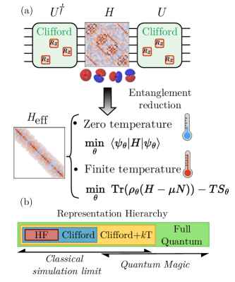
Figure 1: General approach for both zero and finite temperature quantum chemistry powered by quantum magic. Starting with a second quantized Hamiltonian $H$, one can use classical simulable quantum circuits, such as Clifford + $k$Rz circuits, to reduce the entanglement of the Hamiltonian by the basis transformation $H_{\text{eff}}=U^{\dagger}HU$. Increasing $k$ climbs the quantum magic ladder, further reducing the quantumness of the transformed Hamiltonian $H_{\text{eff}}$.

Quantum Chemistry Simulations. One fundamental goal of the electronic structure problem is to solve the energy of the many-body electronic Hamiltonian at zero and finite temperature:

$$H_{\text{elec}}=-\sum_{i}\frac{\nabla_{i}^{2}}{2m_{e}}-\sum_{I,i}\frac{Z_{I}e^{2}}{\absolutevalue{R_{I}-r_{i}}}+\sum_{i,j>i}\frac{e^{2}}{\absolutevalue{r_{i}-r_{j}}},$$ (1)

where $Z_{I}$ is the atomic number, $R_{I}$ is the coordinates of the atoms, $m_{e}$ is the mass of the electron and $r_{i}$ is the coordinates of electrons. To simplify this problem, we start with the Hartree-Fock self-consistent equations, re-expressing the electronic Hamiltonian on the basis of molecular orbitals (MOs):

$$H_{\text{elec}}=\sum_{p,q}h_{pq}\hat{c}^{\dagger}_{p}\hat{c}_{q}+\dfrac{1}{2}\sum_{p,q,r,s}V_{pqrs}\hat{c}^{\dagger}_{p}\hat{c}^{\dagger}_{q}\hat{c}_{s}\hat{c}_{r},$$ (2)

where $p,q,r,s$ label the spin-orbitals and $\hat{c}_{\alpha}$, $\hat{c}^{\dagger}_{\alpha}$ are the annihilation and creation fermionic operators. With a fermion-qubit mapping (e.g., parity mapping [26], Jordan-Wigner [27], Bravyi-Kitaev [28]), we can further map the fermionic Hamiltonian to a qubitized Hamiltonian $H=\sum_{i}\alpha_{i}P^{[\mu_{i}]}$, where $P^{[\mu_{i}]}$ denotes a tensor product of Pauli operators, also known as a Pauli string.

To approximate the ground state of a Hamiltonian $H$, the variational principle is commonly used. In particular, the energy functional $E(\theta)=\expectationvalue{H}{\psi_{\theta}}$ is minimized with respect to parameters $\theta$, which parameterize a quantum state $\ket{\psi_{\theta}}$. This can be realized on near-term quantum computers via VQE [6, 2] and can also generalize to finite temperatures, where the free energy of the Gibbs state is of interest [29]. In this latter application, as the number of electrons fluctuates from environmental interactions [22], the Gibbs state must be modeled as the grand canonical ensemble $\rho=e^{-\beta(H-\mu N)}/\mathcal{Z}$, with inverse temperature $\beta$, chemical potential $\mu$, particle number $N$, and partition function $\mathcal{Z}$. In addition to sampling approaches on the Gibbs distribution [29], the variational free energy principle provides another powerful tool to estimate the (grand) free energy, and can be achieved by minimizing the objective $\beta\textup{tr}(\rho_{\theta}(H-\mu N))+\textup{tr}(\rho_{\theta}\textup{log}\rho_{\theta})$ over a parameterized density matrix $\rho_{\theta}$.

The Quantum Magic Ladder. In what follows, we describe a unified framework for ground state and finite temperature quantum chemistry simulations via Clifford + $k$Rz transformation, where Rz refers to a single qubit z-axis rotational gate. The attractiveness of the Clifford + $k$Rz approach is manifold. Clifford circuits are classically simulable with complexity $O(n^{3})$, where $n$ is the system size. When doped with $k$ non-Clifford gates, this complexity increases by a factor exponential in $k$; therefore, for $k\leq O(\log n)$, we can construct of Clifford + $k$Rz similarity transforms in polynomial time with purely classical resources [21, 30, 31]. The practicality of our approach gains even greater relevance in the early quantum fault-tolerant regime, where the stabilizer formalism of popular quantum error-correcting codes favors Clifford-dominated circuits. Indeed, the Clifford ansatz is a natural step beyond mean-field theory, since the Hartree-Fock (HF) solution in the qubit basis is a product state of 0 and 1, indicating which molecular orbital has been occupied, and rendering the HF solution a special case of the Clifford transformation ansatz.

However, our work exceeds pure Clifford enhancement by incorporating a notion known as quantum magic [19, 20]. Our main insight is that the optimal Clifford + $k$Rz circuit can minimize the quantumness of a Hamiltonian along two axes: reducing 1) its entanglement via the Clifford component of the circuit, and 2) its quantum magic via its non-Clifford components. As we add more Rz gates by increasing the $k$ parameter, we increase the degree to which our transform captures the quantum magic of the energy eigenbasis, a process we refer to as “climbing” the quantum magic ladder. Ultimately, this leads to an approximate diagonalization of the Hamiltonian and suppression of the off-diagonal terms (see Fig. 1). We apply this general approach, not only to ground state simulation, but also to finite temperature calculations [32, 33, 34, 35, 36], and examine how our transformation reduces the complexity of zero and finite temperature quantum simulations.

The general scheme of our approach is described in Fig. 1. Keeping with the similarity transformation methods previously discussed, we identify a a unitary transformation $U$ in the Clifford + $k$Rz ladder such that the resulting Hamiltonian $H_{\text{eff}}=U^{\dagger}HU$ is as close as possible to a diagonal matrix, such that $H_{\text{eff}}$ greatly reduces the quantum resources for zero and finite temperature quantum simulations. If we instead consider the quantum state perspective, this technique is equivalent to searching for a Clifford + $k$Rz unitary transformation $U$ such that $U\ket{0}$ approximates the ground state of the Hamiltonian $H$. Likewise, for finite temperature, the aim is to find a transformation $U$ and a classical distribution $p(x)$ over $x\in\{0,1\}^{n}$ such that the mixed state $\sum_{x\in\{0,1\}^{n}}p(x)U\outerproduct{x}{x}U^{\dagger}$ approximates the thermal state $e^{-\beta(H-\mu N)}/\mathcal{Z}$.

As Rz and T gates have the same simulation complexity [21, 30, 31] and Rz gates strictly generalize T gates, we optimize $U$ in the Clifford + $k$Rz ansatz instead of the conventional Clifford+$k$T ansatz , from which we observe a large performance increase. The simulation of Clifford + $k$Rz circuits was performed using the PyClifford package [38] (details in Appendix A). As $U$ optimization in the Clifford + $k$Rz ladder is a hybrid discrete continuous problem with an enormous search space, we develop a three-step algorithm to address it. First, we observed that the quantum chemistry Hamiltonian in Pauli string form resembles a disordered Hamiltonian with energy coefficients of various scales. As the spectrum bifurcation renormalization group (SBRG) [23, 24, 25] and strong-disorder renormalization group [39, 40, 41] are effective for solving strongly-disordered quantum materials, we deploy the former to warm-start the Clifford transformation. Based on the Clifford circuit given by the SBRG, we perform a combination of greedy search and gradient descent to further $U$ (see Appendix B). While a disadvantage of our approach is that the Clifford + $k$Rz ansatz does not necessarily conserve the Hamiltonian’s symmetries, we observe that, remarkably, our optimization process tends to identify Clifford + $k$Rz circuits that conserve number and spin symmetries (see Appendix C).

Figure 2: Clifford + $k$Rz improvement for LiH and H₂O ground state energies over different bond lengths. As we climb the quantum magic ladder with additional Rz gates, the optimal energy gap reduces. The inset shows the stabilizer Rényi entropy of the ground state and first excited state at different bond lengths, quantifying the quantum magic.

Results. We apply our Clifford+kRz transformation for both ground state and finite temperature quantum chemistry simulations, starting with VQE for LiH and H₂O. In Fig. 2, the optimal energy gap $E-E_{0}$ is plotted as a function of different bond lengths between atoms, where $E$ is the energy optimized from Clifford + $k$Rz transformation and $E_{0}$ is the exact energy. Since the HF solution is a strict subset of the Clifford ansatz, the optimal energy gap of a pure Clifford transformation ($k=0$) is upper bounded by that of the HF solution. However, improvement from pure Clifford circuits only occurs when the bond length exceeds the equilibrium bond length. Climbing higher on the quantum magic ladder, the optimal energy gap significantly reduces for all the bond lengths. Moreover, as the number of non-Clifford gates increases, the optimal energy gap decreases, and entanglement is reduced.

Interestingly, the optimal energy gap peaks around a particular bond length, indicating a region of maximal quantum magic. To quantify the quantum magic, we use stabilizer entropy [42]. One can define a probability of a Pauli string $P$ appearing in the representation of a state $\ket{\psi}$ as $\Xi_{\psi}(P)=\langle\psi|P|\psi\rangle^{2}/2^{n}$. As $\Xi$ forms a valid probability distribution over all $4^{n}$ Pauli strings, the stabilizer entropy $M$ can be defined in terms of the Shannon entropy $H$ of $p_{\psi}$: $M(\ket{\psi})=H(\Xi_{\psi})-n$. It can be shown that $M(\ket{\psi})\geq 0$ and that the inequality is saturated if and only if $\ket{\psi}$ is a stabilizer state [42]. Using $M$ as a measure of quantum magic, we see in the inset of Fig. 2 that quantum magic and the optimal energy gap peak in the same bond length region. This confirms that regions with high quantum magic cannot be well reduced by basis transformations with insufficient non-Clifford gates, as they require more extensive quantum resources. Thus, in regions of high quantum magic, systems with greater expressivity, namely real quantum devices, are required for accurate results.

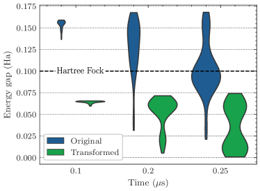
Figure 3: Pulse time reduction with the transformed Hamiltonian. We model an analog quantum machine with a ⁸⁷Rb atomic chain for LiH ground state preparation using fixed lattice spacing and total evolution time. The Rabi frequency and the local detuning of each atom are optimized. The width of features is proportional to the solution density. For each evolution time, twenty randomly initialized VQE are trained.

We further explore this idea for analog quantum computation. As NISQ devices have limited coherence time, we propose our transformation to reduce the entanglement and evolution time of real quantum devices. After our transformation, the remaining structure requires quantum magic, that should be generated by a real quantum computer. Instead of using the digital quantum circuit paradigm, we directly model the physical hardware as programmable quantum simulators (PQS). Specifically, we considered a one-dimensional Rydberg atom chain to model the ground state of LiH. The atoms have lattice spacing $d=9.37\mu\text{m}$ and their interaction strength is that of the $70S_{1/2}$ Rydberg state of ⁸⁷Rb atoms.

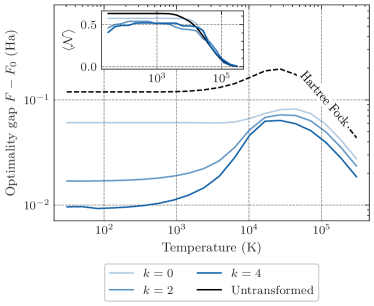
Figure 4: Free energy optimality gap for LiH at a bond length 3.4Å. The inset shows the entanglement negativity $\mathcal{N}$ (Eq. 4) averaged over each site of the Gibbs state for the transformed Hamiltonian.

To show that the transformed Hamiltonian yields better performance for ground state energy estimation, we fix the total PQS evolution time $T$ and train the time-dependent Rabi frequencies $\Omega_{i}(t)$ and local detunings $\Delta_{i}(t)$ of each atom $i$. We model LiH with bond length 3.4Å, which, exhibits high stabilizer entropy (Fig. 2), indicating that additional quantum magic would be beneficial. For each fixed total evolution time $T$, we optimize 20 random initialized VQE runs for both the original and Clifford-transformed Hamiltonians, using automatic differentiation with Jax [43] and Tensorcircuit [44] to directly optimize the pulse shapes. The results are shown in Fig. 3. For $T=0.1\mu$s, we observe that the optimized energy with the original Hamiltonian is concentrated at levels significantly above the HF energy, because the PQS expressivity and entanglement. Conversely, the optimized energy using the transformed Hamiltonian is concentrated at a smaller energy than the HF solution due to entanglement reduction by the Clifford circuit. As the evolution time increases, the PQS generates more quantum magic, further reducing the optimal energy gap. For $T=2.5\mu$s, more than half of the VQE runs trained on $H_{\text{eff}}$ achieve energy gap $\Delta E\leq 0.1$ Hartrees, whereas most VQE instances trained with the original Hamiltonian only slightly outperform the HF energy. This demonstrates that Clifford + $k$Rz transformations effectively reduce entanglement and pulse times, a significant advantage for near-term quantum devices.

For finite temperature calculations, we apply our approach to the LiH molecule for grand free energy estimation. Our ansatz for the density matrix is

$$\rho=\sum_{x\in\{0,1\}^{n}}p(x)U\ket{x}\bra{x}U^{\dagger},$$ (3)

where $U$ is a Clifford + $k$Rz circuit. We minimize the free energy $F=\langle H\rangle-\mu\langle N\rangle-TS$, given the constraint $\Tr(\rho N)=\bar{N}$, where $\bar{N}$ is the number of ground state electrons. Here we solve $p(x)$ exactly for each given $U$. The results in Fig. 4 show that the Clifford + $k$Rz ansatz consistently reduces the optimal free energy gap $F-F_{0}$ as we climb the quantum magic ladder. Likewise, all Clifford transformations outperform the finite temperature HF method, including the pure Clifford transformation ($k=0$), which reduces the optimal free energy gap by $\sim 50\%$. This indicates that the finite temperature density matrix has classically simulable entanglement that is reduced in favorable bases.

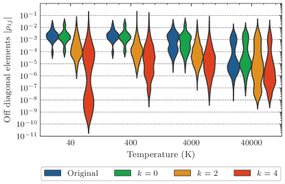
Figure 5: Density distribution of the off-diagonal term for the Gibbs state $\rho$ of LiH across different temperatures for bond length 3.4Å. The width of features is proportional to solution density.

To quantify this, we examine the entanglement and off-diagonal terms for the exact Gibbs state $\rho_{ij}$ post transformation. While there are a number of entanglement measures for mixed states, we choose the entanglement negativity measure [45, 46, 47]:

$$\mathcal{N}(\rho)=\dfrac{||\rho^{\Gamma_{A}}||_{1}-1}{2},$$ (4)

where $\rho^{\Gamma_{A}}$ is the partial transpose of $\rho$ with respect to the subsystem $A$. In the inset of Fig. 4, we show that indeed Clifford + $k$Rz transformations consistently reduce the entanglement negativity of the thermal state. Fig. 5 shows that, across a wide temperature range, our transformation’s minimization of off-diagonal elements in the exact Gibbs state $\rho$ increases with $k$. Since the Gibbs ensemble becomes classical in the limit of negligible off-diagonal terms, this reduction illustrates the power of quantum magic to reduce quantumness in finite temperature simulations.

Conclusions. We have developed a general approach for zero and finite temperature quantum simulations from a quantum information theoretic perspective, facilitated by the Clifford + $k$Rz transformation. One of the primary benefits of our approach is that it is fully classically simulable for small $k$, providing an efficient method to judiciously reduce quantum resources. Furthermore, it produces Clifford-dominated circuits, which are necessary for practical implementation with near-term devices. By initially using Clifford circuits and gradually increasing complexity through non-Clifford operations, we pave a continuous path towards full fault-tolerant quantum computation, forming what we deem a quantum magic ladder. Moreover, we apply our methods in the context of quantum chemistry ground state and free energy calculations, demonstrating superior performance to HF techniques and consistent improvement with increasing quantum magic on both digital and analog quantum computers. We examine how the Clifford + $k$Rz transformation reduces entanglement and quantumness for quantum simulations, and conserving quantum resources. Coupled with our general framework for finite temperature simulations, our approach enables near-term quantum computers to address a wide array of crucial quantum chemistry problems.

Building on this foundation, our framework opens numerous opportunities to advance quantum simulations using quantum magic. Algorithmically, in addition to the greedy search algorithms used in this work, powerful methods such as simulated annealing and differentiable quantum architecture search [48] could be considered. To scale finite temperature calculations to larger systems, high-dimensional classical probability distributions of the Gibbs state can be simulated using generative models in the spirit of $\beta$-VQE [49]. Our approach can also be applied to the finite temperature calculation based on the thermal double field framework [50, 51]. These methodologies offer promising pathways to tailor our transformations to specific applications, providing efficient and robust solutions to complex quantum problems. In summary, our Clifford + $k$Rz transformation offers insights and versatile new techniques suitable for diverse quantum simulations, laying a practical foundation for future breakthroughs in quantum simulation.

Acknowledgement. The authors would like to thank Chong Sun, Yi Tan, Linqing Peng, Yuan Liu, Shi-Xin Zhang and Ryan Babbush for the helpful discussion. DL acknowledges support from the NSF AI Institute for Artificial Intelligence and Fundamental Interactions (IAIFI). This material is based upon work supported by the U.S. Department of Energy, Office of Science, National Quantum Information Science Research Centers, Co-design Center for Quantum Advantage (C2QA) under contract number DE-SC0012704. HYH is grateful for the support from Harvard Quantum Initiative Fellowship. SFY would like to thank the NSF through a Cornell HDR and the CUA PFC grant.

Supplementary Material

Appendix A Classical simulation of Clifford-dominated quantum circuits

In this section, we review the basic idea of the generalized stabilizer representation and how to simulate non-Clifford gates and general quantum states with stabilizer frames. First, let us define Pauli group and stabilizer group:

Definition A.1 (Pauli group)

The Pauli group on n-qubits is the set of all tensor products of Pauli matrices, i.e.

$$G_{n}=\{i^{k}\sigma^{i_{1}}\otimes\sigma^{i_{2}}\otimes\cdots\otimes\sigma^{i_{n}}|k,i_{h}\in\{0,1,2,3\}\}$$ (5)

Definition A.2 (Stabilizer group)

Stabilizer group $\mathcal{S}$ is a subgroup of Pauli group satisfies the following properties:
1. $\mathcal{S}$ is an abelian group. For $\forall s_{i},s_{j}\in\mathcal{S}$, $[s_{i},s_{j}]=0$.
2. It doesn’t contain negative identity, i.e. $-I\notin\mathcal{S}$.

The stabilizer group can always be represented by its generators. For example, a stabilizer group containing $2^{r}$ elements can be represented by $r$ generators of the group: $\mathcal{S}=\langle s_{1},s_{2},\dots,s_{r}\rangle$. One should notice the generators are not unique. For example, $\mathcal{S}=\langle s_{1},s_{2},\dots,s_{r}\rangle=\langle s_{1}s_{2},s_{2},\dots,s_{r}\rangle$. With the stabilizer group, one can define stabilizer states:

Theorem A.1 (Pure stabilizer state)

A full stabilizer (n generators for a n-qubit system) stabilizes a unique pure state $\ket{\psi_{S}}$

One can check the density matrix can be represented as

$$\rho_{S}=\dfrac{1}{2^{n}}\prod_{i=1}^{n}\left(I+s_{i}\right)$$ (6)

Another concept that is useful for describing general quantum state is the destabilizers:

Definition A.3 (Destabilizer group)

A destabilizer group $\mathcal{D}$ is a subgroup of Pauli group associated with the stabilizer group $\mathcal{S}=\langle s_{1},s_{2},\dots,s_{r}\rangle$. It has the following properties:
1. $\mathcal{D}$ has the same number of generators as $\mathcal{S}$: $\mathcal{D}=\langle d_{1},d_{2},\dots,d_{r}\rangle$.
2. For each generator $d_{i}$, it anti-commute with $s_{i}$, but commute with all the other generators $s_{j},j\neq i$.

Definition A.4 (Full tableau)

A full stabilizer tableau $\mathcal{T}=(\mathcal{S},\mathcal{D})$ is a pair of full stabilizer and destabilizer.

Definition A.5 (Stabilizer basis)

The stabilizer basis with full tableau $\mathcal{T}$ is $\mathcal{B}(\mathcal{T})=\{d\ket{\psi_{S}}|d\in\mathcal{D}\}$

The stabilizer basis is an orthonormal and complete basis for $n$-qubit Hilbert space. Since the destabilizers are note unique, if $\mathcal{D}$ and $\mathcal{D}^{\prime}$ are both destabilizers for $\mathcal{S}$, then $\mathcal{B}(S,D)$ and $\mathcal{B}(S,D^{\prime})$ are the same set of basis modulo phase difference. Since $\mathcal{B}(\mathcal{T})$ is a complete basis for Hilbert space, then any quantum state can be represented by the stabilizer basis. Therefore, we introduce the generalized stabilizer representation.

Definition A.6 (Generalized stabilizer representation)

Any pure quantum state can be represented with stabilizer basis. More particularly, the density matrix $\rho$ of any pure quantum state can be written as

$$\rho=\sum_{i=1}^{2^{n}}\sum_{j=1}^{2^{n}}\chi_{ij}d_{i}\ket{\psi_{S}}\bra{\psi_{S}}d_{j}=\sum_{ij}\chi_{ij}d_{i}\rho_{S}d_{j}.$$ (7)

Therefore, we call the two-tuple $(\chi,\mathcal{B}(\mathcal{S},\mathcal{D}))$ the generalized stabilizer representation.

For a general state, in the worst case, we need $\mathcal{O}(4^{n})$ classical memory to store and simulate its dynamics. However, this formulation is particularly useful when this decomposition is sparse. For simplicity, we can use the zero norm of $\chi$ matrix to denote its complexity, i.e. $\Lambda(\chi)=||\chi||_{0}$. And the simulation complexity scales as $\mathcal{O}(\Lambda(\chi))$. Now we define the Pauli channel and see how to simulate general quantum states with the generalized stabilizer representation.

Definition A.7 (Pauli channel)

The Pauli channel of a n-qubit system can be written as

$$\mathcal{E}(\rho)=\sum_{ij}\phi_{ij}P_{i}\rho P_{j}$$ (8)

where $P_{i},P_{j}\in G_{n}$, and $\phi_{ij}$ are complex numbers. We use $\Lambda(\mathcal{E})=||\phi||_{0}$ to denote the complexity of the Pauli channel.

A.1 General state evolution under Clifford gates

The evolution of the general state under a Clifford circuit $C$ evolution can be written as

$$C\rho C^{\dagger}=C\left(\sum_{ij}\chi_{ij}d_{i}\rho_{S}d_{j}\right)C^{\dagger}=\sum_{ij}\chi_{ij}Cd_{j}C^{\dagger}\left(C\rho_{S}C^{\dagger}\right)Cd_{j}C^{\dagger}$$ (9)

Therefore, we only need to update the full tableau $\mathcal{T}=(\mathcal{S},\mathcal{D})$, which can be done with $\mathcal{O}(n^{2})$ time. Under Clifford gates, the general stabilizer frame will update as $(\chi,\mathcal{S},\mathcal{D})\rightarrow(\chi,\mathcal{S}^{\prime},\mathcal{D}^{\prime})$.

A.2 General state evolution under Pauli channels

First, we use the fact that any Pauli string can be decomposed with stabilizer and destabilizers, $P_{m}=\alpha_{m}d_{b_{m}}s_{c_{m}}$. An efficient implementation of this decomposition is in Algorithm 1. Suppose we want to simulate a general Pauli channel, $\mathcal{E}(\rho)=\sum_{m,n}\phi_{m,n}P_{m}\rho P_{n}^{\dagger}$. For each term in the Pauli channel:

$$\begin{split}\phi_{m,n}P_{m}\rho P_{n}^{\dagger}&=\sum_{ij}\phi_{m,n}P_{m}\chi_{ij}d_{i}\rho_{S}d_{j}P_{n}^{\dagger}=\sum_{ij}\phi_{m,n}\chi_{ij}P_{m}d_{i}\rho_{S}d_{j}P_{n}^{\dagger}\\ &=\sum_{ij}\phi_{m,n}\chi_{ij}\alpha_{m}\alpha^{*}_{n}d_{b_{m}}s_{c_{m}}d_{i}\rho_{S}d_{j}s_{c_{n}}d_{b_{n}}\\ &=\sum_{ij}\phi_{m,n}\chi_{ij}\alpha_{m}\alpha^{*}_{n}(-1)^{c_{m}\cdot i+c_{n}\cdot j}d_{b_{m}}d_{i}s_{c_{m}}\rho_{S}s_{c_{n}}d_{j}d_{b_{n}}\\ &=\sum_{ij}\left(\phi_{m,n}\chi_{ij}\alpha_{m}\alpha^{*}_{n}(-1)^{c_{m}\cdot i+c_{n}\cdot j}\right)d_{b_{m}+i}\rho_{S}d_{j+b_{n}}\\ &=\sum_{i^{\prime}j^{\prime}}\chi^{\prime}_{i^{\prime}j^{\prime}}d_{i^{\prime}}\rho_{S}d_{j^{\prime}}.\end{split}$$ (10)

Therefore, for each term in Pauli channel, we need to update $(\chi,\mathcal{S},\mathcal{D})\rightarrow(\chi^{\prime},\mathcal{S},\mathcal{D})$. And we sum over all the terms in the Pauli channel, which contains $\Lambda(\phi)$ terms. Especially, T-gate can be written as the following channel:

$$\begin{split}T\rho T^{\dagger}=\left(\cos\dfrac{\pi}{8}I+i\sin\dfrac{\pi}{8}Z\right)\rho\left(\cos\dfrac{\pi}{8}I-i\sin\dfrac{\pi}{8}Z\right)\end{split},$$ (11)

where $\Lambda(T)=4$.

Algorithm 1 Pauli decomposition algorithm

1:procedure Decompose($P$)$\rightarrow\alpha\mathbf{d}_{b}\mathbf{s}_{c}$

2:     Initialize zero vector $\mathbf{b}=(0,\dots,0)$, and $\mathbf{c}=(0,\dots,0)$

3:     phase = 0

4:     $P_{t}=I$ $\triangleright$ binary vector encoding, no phase information.

5:     for $i=0,i<N,i++$ do $\triangleright$ Loop over stabilizer generators

6:         if $\{P,\mathbf{s}_{i}\}=0$ then

7:              $b_{i}=1$

8:              $\text{phase}-=\text{ipow}(P_{t},\mathbf{d}_{i})$

9:              $P_{t}=P_{t}*\mathbf{d}_{i}$

10:         end if

11:     end for

12:     for $i=0,i<N,i++$ do $\triangleright$ Loop over destabilizer generators

13:         if $\{P,\mathbf{d}_{i}\}=0$ then

14:              $c_{i}=1$

15:              $\text{phase}-=\text{ipow}(P_{t},\mathbf{s}_{i})$

16:              $P_{t}=P_{t}*\mathbf{s}_{i}$

17:         end if

18:     end for

19:     return phase, $\mathbf{b}$, and $\mathbf{c}$.

20:end procedure

Appendix B Optimization of Clifford+$k$Rz circuits

We use a brickwork circuit ansatz (see Fig. 6) with $L$ layers. One layer is composed of $n$ Clifford gates, each of which acts on neighboring qubits. Although a common gate set for the Clifford group is taken to be the Hadamard, phase, and CNOT gates, we instead use the gate set composed of $e^{i\pi P/4}$, where $P\in\{I,X,Y,Z\}^{\otimes 2}$. We dope the circuit with $k$ Rz gates at a fixed layer, but a variable site index (which is optimized over). To summarize, our free parameters belong to the domain $\mathbb{Z}_{16}^{n\times L}\times\mathbb{Z}_{n}^{k}\times\mathbb{R}^{k}$. The first term corresponds to 16 possible choices for the Clifford gates (of which there are $n\times L$). The second corresponds to the $n$ possible choices for the site index of the $k$ Rz gates, and the last is simply the argument for the $k$ Rz gates.

@C=1.0em @R=0.2em @!R
q_0 : & q_0 : 1e^i πP_0 /4 $e^{i\pi P_{4}/4}$ [0em]7 [0em]7 1e^i πP_8 /4 $e^{i\pi P_{12}/4}$
q_1 : q_1 : e^i πP_0 /4 1e^i πP_5 /4 e^i πP_8 /4 1e^i πP_13 /4
q_2 : q_2 : 1e^i πP_1 /4 e^i πP_5 /4 R_z(θ_0) 1e^i πP_9 /4 e^i πP_13 /4
q_3 : q_3 : e^i πP_1 /4 1e^i πP_6 /4 e^i πP_9 /4 1e^i πP_14 /4
q_4 : q_4 : 1e^i πP_2 /4 e^i πP_6 /4 1e^i πP_10 /4 e^i πP_14 /4
q_5 : q_5 : e^i πP_2 /4 1e^i πP_7 /4 R_z(θ_1) e^i πP_10 /4 1e^i πP_15 /4
q_6 : q_6 : 1e^i πP_3 /4 e^i πP_7 /4 1e^i πP_11 /4 e^i πP_15 /4
q_7 : q_7 : e^i πP_3 /4 $e^{i\pi P_{4}/4}$ e^i πP_11 /4 $e^{i\pi P_{12}/4}$

Figure 6: The brickwork circuit ansatz for $L=2$ and $k=2$.

To optimize our circuit, we treat the discrete and continuous parameters separately. We label $X\in\mathbb{Z}_{16}^{n\times L}\times\mathbb{Z}_{n}^{k}$ the discrete parameters and $\Theta\in\mathbb{R}^{k}$ the continuous ones. For any cost function $f(X,\Theta)$, we can define a ‘marginalized’ cost function by minimizing over $\Theta$:

$$f(X)\equiv\min_{\Theta}f(X,\Theta).$$ (12)

This is a useful construction when it is easy to do this minimization; it turns out that for small $k$, this process is very easy. Since the cost is periodic in $\Theta$, we only need to search the small volume $\Theta\in[0,2\pi]^{k}$. This search is further simplified by the fact that $f(X,\Theta)$ is continuous in $\Theta$, and does not have many local minima (see Fig. 7). By applying a simple gradient-based optimizer (e.g., gradient descent, conjugate gradient, etc.) to just a few ($\sim 10$) randomly initialized choices of $\Theta$, we can often find the global minimum within very few iterations. This is to say, the marginalized cost function $f(X)$ is easy to evaluate. With this, we optimize over the remaining parameters $X$ with a simple greedy search. Each iteration, we pick one of the parameters in $X$ to optimize over. For instance, if we choose to optimize $P_{1}$ (refer to Fig. 6), we would evaluate the cost with all other parameters held constant, varying $P_{1}$ over all 16 possibilities $\{I,X,Y,Z\}^{\otimes 2}$. Then, we simply replace $P_{1}$ with the choice that yielded the lowest cost $f(X)$. Finally, we do this discrete optimization in parallel for a large number ($n_{init}\sim 1000$) of randomly initialized parameters $X$, and simply take the best performing solution after a fixed number ($n_{iter}\sim 100$) iterations. Although we considered more advanced schemes for this discrete optimization, such as a simulated annealing process, we found that these schemes did not yield better results.

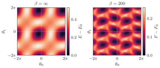
Figure 7: The landscape of $f(\Theta)\equiv f(X_{best},\Theta)$ for LiH at a bond length $3.4$Å, where $X_{best}$ was the best performing solution for $k=2$. On the left, we show the landscape for the ground state calculation, and on the right, we show the landscape at a finite temperature $\beta=200$ ($T\approx 1500\text{K}$). Note that there are very few suboptimal local minima – applying gradient descent to a randomly initialized $\Theta$ will find the global minimum with high probability.

Algorithm 2 Optimizing Clifford + $k$Rz Circuits

procedure Optimize($f,L,k,n_{iter}$)

     $X\leftarrow$ random initialization in $\mathbb{Z}_{16}^{n\times L}\times\mathbb{Z}_{n}^{k}$

     for $i=1,\ldots,n_{iter}$ do

         $j\leftarrow$ random index in $1,\ldots,n\cdot L+k$

         if $j\leq n\cdot L$ then

              $params\leftarrow\mathbb{Z}_{16}$

         else

              $params\leftarrow\mathbb{Z}_{n}$

         end if

         for $p\in params$ do

              $X[j]\leftarrow p$

              $\text{cost}[p]\leftarrow f(X)$

         end for

         $X[j]\leftarrow\text{argmin}_{p}\text{cost}[p]$

     end for

end procedure

Appendix C Symmetry of the Recovered Solutions

A noteworthy drawback of the Clifford + $k$Rz ansatz (Fig. 6) is that it does not necessarily conserve any symmetries of the Hamiltonian. Despite this, we observe that the optimization process prefers to recover solutions that are both eigenstates of the number and spin operators, and furthermore, typically states that conserve symmetries in the Hamiltonian (e.g., total spin zero). Although observe that the latter does not hold for every solution (see Fig. 9), it holds in the vast majority of cases. Remarkably, we observe a greater tendency to preserve symmetries as more Rz gates are injected.

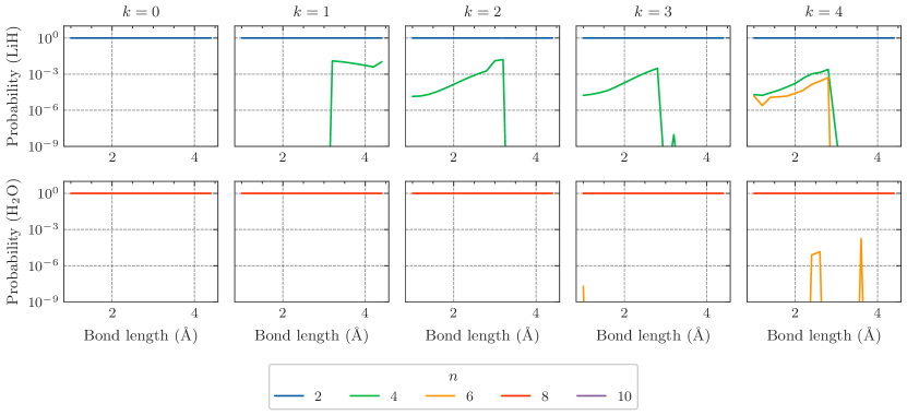
Figure 8: We analyze optimized Clifford + $k$Rz solution in the eigenbasis for the qubitized number operator $N$ for both LiH (top) and H₂O (bottom), demonstrating that the recovered solution approximately conserves of $N$.

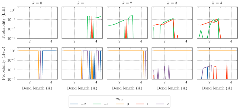
Figure 9: We analyze optimized Clifford + $k$Rz solution in the eigenbasis for the qubitized spin operator $S$ for both LiH (top) and H₂O (bottom), demonstrating that the recovered solution, for most cases, approximately conserves of $S$.

Appendix D Pulse optimization of programmable quantum simulators

The Rydberg Hamiltonian can be modeled as

$$\begin{split}H/\hbar=\sum_{j}\dfrac{\Omega_{j}(t)}{2}\left(e^{\mathrm{i}\phi_{j}(t)}\ket{g}\bra{r}+e^{-\mathrm{i}\phi_{j}(t)}\ket{r}\bra{g}\right)-\sum_{j}\Delta_{j}(t)\hat{n}_{j}+V_{ij}\hat{n}_{i}\hat{n}_{j},\end{split}$$ (13)

where $\Omega_{j}(t)$, $\phi_{j}(t)$, $\Delta_{j}(t)$ are Rabi frequency, laser phase, and local detuning of the driving field for each atom, and $\ket{g}$ is the ground state, $\ket{r}$ is the Rydberg state, $\hat{n}_{j}=\ket{r}_{j}\bra{r}_{j}$ is the number operator. We use $V_{ij}=C_{6}/|x_{i}-x_{j}|^{6}$ with $C_{6}=2\pi*8.627*10^{5}~{}\text{MHz}~{}\mu m^{6}$ to describe the Rydberg interactions. In our optimization, we translate the Hamiltonian into Pauli basis, which gives

$$\begin{split}H/\hbar=\sum_{j}\left(\dfrac{\Omega_{j}}{2}\cos\phi_{j}X_{j}-\dfrac{\Omega_{j}}{2}\sin\phi_{j}Y_{j}\right)+\sum_{j}\left(\dfrac{\Delta_{j}}{2}-V_{ij}\right)Z_{j}+\sum_{i,j}\dfrac{V_{ij}}{4}Z_{i}Z_{j}+H_{\text{const}},\end{split}$$ (14)

where $H_{\text{const}}=\sum_{i,j}\frac{V_{ij}}{4}I-\sum_{j}\frac{\Delta_{j}}{2}I$. Then we optimize the pulse in the Pauli basis, such as $\frac{\Omega_{j}}{2}\cos\phi_{j}$. We parameterize each pulse as a piece-wise constant function with ten pieces, and initialize them randomly. The atom positions are fixed to be separated with 9.37$\mu m$. Since the interaction strength of the next nearest neighbors are 64 times smaller than the interaction strength of the nearest neighbors, we only consider the leading nearest neighbor interactions for our model.

Appendix E Finite temperature calculation

The variational principle extends beyond ground state calculations; indeed, it can be shown that the free energy satisfies a variational principle. That is, defining

$$F_{\beta}(\rho)\equiv\Tr(H\rho)-S(\rho)/\beta,$$ (15)

where $S(\rho)$ is the von Neumann entropy, it can be shown that for all $\beta$,

$$F_{\beta}(\rho)\geq F_{\beta}\quantity(\frac{e^{-\beta H}}{\Tr(e^{-\beta H})})\equiv F_{0}$$ (16)

for all $\rho$. We take advantage of this variational principle to estimate the free energy at finite temperatures. The procedure is simple: we fix an orthogonal basis of stabilizer states $\quantity{\ket{\psi_{k}}\mid k=1,\ldots,2^{n}}$ (typically derived from SBRG), so that the initial state is

$$\rho_{0}\equiv\sum_{k}p_{k}\outerproduct{\psi_{k}}{\psi_{k}},$$ (17)

where the $p_{k}\in[0,1]$ form a probability distribution (i.e., $\sum_{k}p_{k}=1$). We construct a Clifford+kRz unitary $U$ from Clifford + $k$T gates, and evolve each of the under this unitary. The final state is therefore

$$\rho=\sum_{k}p_{k}U\outerproduct{\psi_{k}}{\psi_{k}}U^{\dagger}.$$ (18)

Defining $E_{k}\equiv\Tr((H-\mu N)U\outerproduct{\psi_{k}}{\psi_{k}}U^{\dagger})$, we observe that

$$F_{\beta}(\rho)=\sum_{k}p_{k}\quantity(E_{k}-\frac{\log p_{k}}{\beta}).$$ (19)

The optimal $p_{k}$ can be solved for in closed form (i.e., they do not need to be optimized numerically), yielding a free energy estimate

$$F_{\beta}(\rho)=-\frac{1}{\beta}\log(\sum_{k}\exp(-\beta E_{k})).$$ (20)

Since calculating $E_{k}$ as a function of the unitary $U$ is efficient, we can then apply our optimization techniques over the unitary $U$ to minimize $F_{\beta}(\rho)$.

References

- Semeghini et al. [2021] G. Semeghini, H. Levine, A. Keesling, S. Ebadi, T. T. Wang, D. Bluvstein, R. Verresen, H. Pichler, M. Kalinowski, R. Samajdar, A. Omran, S. Sachdev, A. Vishwanath, M. Greiner, V. Vuletić, and M. D. Lukin, Science 374, 1242 (2021), https://www.science.org/doi/pdf/10.1126/science.abi8794 .
- Cerezo et al. [2021] M. Cerezo, A. Arrasmith, R. Babbush, S. C. Benjamin, S. Endo, K. Fujii, J. R. McClean, K. Mitarai, X. Yuan, L. Cincio, and P. J. Coles, Nature Reviews Physics 3, 625 (2021).
- Georgescu et al. [2014] I. M. Georgescu, S. Ashhab, and F. Nori, Rev. Mod. Phys. 86, 153 (2014).
- Cao et al. [2019] Y. Cao, J. Romero, J. P. Olson, M. Degroote, P. D. Johnson, M. Kieferová, I. D. Kivlichan, T. Menke, B. Peropadre, N. P. D. Sawaya, S. Sim, L. Veis, and A. Aspuru-Guzik, Chemical Reviews, Chemical Reviews 119, 10856 (2019).
- Bauer et al. [2020] B. Bauer, S. Bravyi, M. Motta, and G. K.-L. Chan, Chemical Reviews, Chemical Reviews 120, 12685 (2020).
- Peruzzo et al. [2014] A. Peruzzo, J. McClean, P. Shadbolt, M.-H. Yung, X.-Q. Zhou, P. J. Love, A. Aspuru-Guzik, and J. L. O’Brien, Nature Communications 5, 4213 (2014).
- Yuan et al. [2019] X. Yuan, S. Endo, Q. Zhao, Y. Li, and S. C. Benjamin, Quantum 3, 191 (2019).
- Liu et al. [2019] J.-G. Liu, L. Mao, P. Zhang, and L. Wang, arXiv e-prints , arXiv:1912.11381 (2019), arXiv:1912.11381 [quant-ph] .
- Kang et al. [2022] C. Kang, N. P. Bauman, S. Krishnamoorthy, and K. Kowalski, Journal of Chemical Theory and Computation, Journal of Chemical Theory and Computation 18, 6567 (2022).
- Mohammadbagherpoor et al. [2019] H. Mohammadbagherpoor, Y.-H. Oh, P. Dreher, A. Singh, X. Yu, and A. J. Rindos, in 2019 IEEE International Conference on Rebooting Computing (ICRC) (2019) pp. 1–9.
- Smith et al. [2022] J. G. Smith, C. H. W. Barnes, and D. R. M. Arvidsson-Shukur, Phys. Rev. A 106, 062615 (2022).
- Roussy [1973] G. Roussy, Molecular Physics 26, 1085 (1973).
- Cederbaum et al. [1989] L. S. Cederbaum, J. Schirmer, and H. D. Meyer, Journal of Physics A: Mathematical and General 22, 2427 (1989).
- Bravyi et al. [2011] S. Bravyi, D. P. DiVincenzo, and D. Loss, Annals of Physics 326, 2793 (2011).
- White [2002] S. R. White, The Journal of Chemical Physics 117, 7472 (2002).
- Mishmash et al. [2023] R. V. Mishmash, T. P. Gujarati, M. Motta, H. Zhai, G. Kin-Lic Chan, and A. Mezzacapo, arXiv e-prints , arXiv:2301.07726 (2023), arXiv:2301.07726 [quant-ph] .
- Ravi et al. [2022] G. S. Ravi, P. Gokhale, Y. Ding, W. Kirby, K. Smith, J. M. Baker, P. J. Love, H. Hoffmann, K. R. Brown, and F. T. Chong, in Proceedings of the 28th ACM International Conference on Architectural Support for Programming Languages and Operating Systems, Volume 1 (2022) pp. 15–29.
- Shang et al. [2023] Z.-X. Shang, M.-C. Chen, X. Yuan, C.-Y. Lu, and J.-W. Pan, Phys. Rev. Lett. 131, 060406 (2023).
- Howard and Campbell [2017] M. Howard and E. Campbell, Physical review letters 118, 090501 (2017).
- Seddon and Campbell [2019] J. R. Seddon and E. T. Campbell, Proceedings of the Royal Society A 475, 20190251 (2019).
- Aaronson and Gottesman [2004] S. Aaronson and D. Gottesman, Phys. Rev. A 70, 052328 (2004).
- Kardar [2007] M. Kardar, Statistical physics of particles (Cambridge University Press, 2007).
- You et al. [2016] Y.-Z. You, X.-L. Qi, and C. Xu, Phys. Rev. B 93, 104205 (2016).
- Duque et al. [2021] C. M. Duque, H.-Y. Hu, Y.-Z. You, V. Khemani, R. Verresen, and R. Vasseur, Phys. Rev. B 103, L100207 (2021).
- Slagle et al. [2016] K. Slagle, Y.-Z. You, and C. Xu, Phys. Rev. B 94, 014205 (2016).
- Seeley et al. [2012] J. T. Seeley, M. J. Richard, and P. J. Love, The Journal of Chemical Physics 137, 224109 (2012), https://pubs.aip.org/aip/jcp/article-pdf/doi/10.1063/1.4768229/13999577/224109_1_online.pdf .
- Jordan and Wigner [1928] P. Jordan and E. P. Wigner, Z. Phys. 47, 631 (1928).
- Tranter et al. [2015] A. Tranter, S. Sofia, J. Seeley, M. Kaicher, J. McClean, R. Babbush, P. V. Coveney, F. Mintert, F. Wilhelm, and P. J. Love, International Journal of Quantum Chemistry 115, 1431 (2015), https://onlinelibrary.wiley.com/doi/pdf/10.1002/qua.24969 .
- Chowdhury and Somma [2016] A. N. Chowdhury and R. D. Somma, “Quantum algorithms for gibbs sampling and hitting-time estimation,” (2016), arXiv:1603.02940 [quant-ph] .
- Bravyi and Gosset [2016] S. Bravyi and D. Gosset, Phys. Rev. Lett. 116, 250501 (2016).
- Bravyi et al. [2022] S. Bravyi, D. Gosset, and Y. Liu, Phys. Rev. Lett. 128, 220503 (2022).
- Zhang and Li [2010] G. Zhang and B. Li, Nanoscale 2 7, 1058 (2010).
- Brown et al. [2016] B. J. Brown, D. Loss, J. K. Pachos, C. N. Self, and J. R. Wootton, Rev. Mod. Phys. 88, 045005 (2016).
- Donoghue et al. [1985] J. F. Donoghue, B. R. Holstein, and R. Robinett, Annals of Physics 164, 233 (1985).
- Sun et al. [2021] S.-N. Sun, M. Motta, R. N. Tazhigulov, A. T. Tan, G. K.-L. Chan, and A. J. Minnich, PRX Quantum 2, 010317 (2021).
- Powers et al. [2023] C. Powers, L. Bassman Oftelie, D. Camps, and W. A. de Jong, Scientific reports 13, 1986 (2023).
- Note [1] The complexity is the same for strong simulation of quantum circuits. See Appendix A for more details.
- Hu et al. [2023] H.-Y. Hu, C. Zhao, T. L. Patti, A. Gu, Y.-Z. You, and S. Yelin, In preparation (2023).
- Khemani et al. [2016] V. Khemani, F. Pollmann, and S. L. Sondhi, Phys. Rev. Lett. 116, 247204 (2016).
- Yu et al. [2019] X. Yu, D. Pekker, and B. K. Clark, arXiv e-prints , arXiv:1909.11097 (2019), arXiv:1909.11097 [cond-mat.str-el] .
- Lim and Sheng [2016] S. P. Lim and D. N. Sheng, Phys. Rev. B 94, 045111 (2016).
- Leone et al. [2022] L. Leone, S. F. Oliviero, and A. Hamma, Physical Review Letters 128 (2022), 10.1103/physrevlett.128.050402.
- Bradbury et al. [2018] J. Bradbury, R. Frostig, P. Hawkins, M. J. Johnson, C. Leary, D. Maclaurin, G. Necula, A. Paszke, J. VanderPlas, S. Wanderman-Milne, and Q. Zhang, “JAX: composable transformations of Python+NumPy programs,” (2018).
- Zhang et al. [2023] S.-X. Zhang, J. Allcock, Z.-Q. Wan, S. Liu, J. Sun, H. Yu, X.-H. Yang, J. Qiu, Z. Ye, Y.-Q. Chen, C.-K. Lee, Y.-C. Zheng, S.-K. Jian, H. Yao, C.-Y. Hsieh, and S. Zhang, Quantum 7, 912 (2023).
- Peres [1996] A. Peres, Physical Review Letters 77, 1413 (1996).
- Eisert and Plenio [1999] J. Eisert and M. B. Plenio, Journal of Modern Optics 46, 145 (1999).
- Horodecki et al. [1996] M. Horodecki, P. Horodecki, and R. Horodecki, “Separability of mixed quantum states: necessary and sufficient conditions phys,” (1996).
- Zhang et al. [2022] S.-X. Zhang, C.-Y. Hsieh, S. Zhang, and H. Yao, Quantum Science and Technology 7, 045023 (2022).
- Liu et al. [2021] J.-G. Liu, L. Mao, P. Zhang, and L. Wang, Machine Learning: Science and Technology 2, 025011 (2021).
- Takahashi and Umezawa [1996] Y. Takahashi and H. Umezawa, International journal of modern Physics B 10, 1755 (1996).
- Wu and Hsieh [2019] J. Wu and T. H. Hsieh, Physical Review Letters 123 (2019), 10.1103/physrevlett.123.220502.