A Measurement of Gravitational Lensing of the Cosmic Microwave Background Using SPT-3G 2018 Data

Abstract

We present a measurement of gravitational lensing over 1500 deg² of the Southern sky using SPT-3G temperature data at 95 and 150 GHz taken in 2018. The lensing amplitude relative to a fiducial Planck 2018 Lambda-Cold Dark Matter ($\Lambda$CDM) cosmology is found to be $1.020\pm 0.060$, excluding instrumental and astrophysical systematic uncertainties. We conduct extensive systematic and null tests to check the robustness of the lensing measurements, and report a minimum-variance combined lensing power spectrum over angular multipoles of $50<L<2000$, which we use to constrain cosmological models. When analyzed alone and jointly with primary cosmic microwave background (CMB) spectra within the $\Lambda$CDM model, our lensing amplitude measurements are consistent with measurements from SPT-SZ, SPTpol, ACT, and Planck. Incorporating loose priors on the baryon density and other parameters including uncertainties on a foreground bias template, we obtain a $1\sigma$ constraint on $\sigma_{8}\Omega_{\rm m}^{0.25}=0.595\pm 0.026$ using the SPT-3G 2018 lensing data alone, where $\sigma_{8}$ is a common measure of the amplitude of structure today and $\Omega_{\rm m}$ is the matter density parameter. Combining SPT-3G 2018 lensing measurements with baryon acoustic oscillation (BAO) data, we derive parameter constraints of $\sigma_{8}=0.810\pm 0.033$, $S_{8}\equiv\sigma_{8}(\Omega_{\rm m}/0.3)^{0.5}=0.836\pm 0.039$, and Hubble constant $H_{0}=68.8^{+1.3}_{-1.6}$ km s^-1 Mpc^-1. Our preferred $S_{8}$ value is higher by 1.6 to 1.8$\sigma$ compared to cosmic shear measurements from DES-Y3, HSC-Y3, and KiDS-1000 at lower redshift and smaller scales. We combine our lensing data with CMB anisotropy measurements from both SPT-3G and Planck to constrain extensions of $\Lambda$CDM. Using CMB anisotropy and lensing measurements from SPT-3G only, we provide independent constraints on the spatial curvature of $\Omega_{K}=0.014^{+0.023}_{-0.026}$ (95% C.L.) and the dark energy density of $\Omega_{\Lambda}=0.722^{+0.031}_{-0.026}$ (68% C.L.). When combining SPT-3G lensing data with SPT-3G CMB anisotropy and BAO data, we find an upper limit on the sum of the neutrino masses of $\sum m_{\nu}<0.30$ eV (95% C.L.). Due to the different combination of angular scales and sky area, this lensing analysis provides an independent check on lensing measurements by ACT and Planck.

I Introduction

Photons from the cosmic microwave background (CMB) are deflected by the intervening gravitational potentials of the large-scale structure (LSS) as they travel to us from the surface of last scattering [e.g., 1]. The distortion of the primordial CMB by gravitational lensing provides a unique way to map the projected matter distribution of the universe, as lensing introduces correlations between CMB fluctuations on different angular scales. We can leverage these correlations to reconstruct the underlying projected matter over- and under-densities and measure the CMB lensing potential power spectrum, from which we can infer the underlying matter power spectrum. Thanks to the high redshift ($z\simeq 1100$) of the CMB, lensing measurements contain LSS information from the last scattering surface to the present day, with the maximum of the lensing kernel around redshift of 2. Lensing measurements can therefore probe the large-scale structure and can inform many key topics in cosmology, including the amplitude of matter density fluctuations [2, 3], the mass of the neutrinos [4, 5, 6, 7, 8], the nature of dark energy [9], and gravity [10, 11, 12, 13].

Lensing measurements have been made with data from several experiments, including ACT [14, 15, 16, 3], BICEP/Keck [17, 18], Planck [19, 20, 21, 22], POLARBEAR [23, 24], and SPT [25, 26, 27, 28, 29, 30]. The tightest lensing amplitude measurements currently come from the DR6 dataset by Advanced ACT [ACT hereafter; 2.3%, 3] and from Planck NPIPE maps [2.4%, 22].

This work presents the first lensing measurement from SPT-3G, the current camera on the South Pole Telescope, using data taken during the abbreviated 2018 season when only a subset of the detectors in the focal plane were fully operational. CMB primary anisotropy cosmology results from the SPT-3G 2018 data are published in Dutcher et al. [31, hereafter D21] and Balkenhol et al. [32, 33].

The focuses of this paper are lensing power spectrum measurements from the SPT-3G 2018 data and their cosmological implications, though we also show the reconstructed lensing maps. Compared to previous SPT lensing measurements, our input maps have higher noise than those used in the SPTpol measurements presented in Wu et al. [28, hereafter W19] and cover a smaller patch than the temperature-only SPT-SZ measurements in Omori et al. [27, hereafter O17]. We use temperature data for this lensing reconstruction, and the resulting SPT-3G lensing map’s $S/N$ per mode is lower than that from SPTpol and higher than that from SPT-SZ. However, because of the larger area of SPT-3G compared to SPTpol and lower noise compared to SPT-SZ, we are able to constrain the lensing amplitude with uncertainties similar to both previous measurements at $\simeq$6%.

With this stringent lensing measurement, the SPT-3G 2018 data already enables competitive constraints on cosmological parameters, alone and in combination with external datasets. The constraints are particularly interesting in light of the current tensions in cosmology, in which cosmological parameters inferred using different probes, each with high precision, do not agree with each other. Specifically, measurements of $H_{0}$ from the Cepheid-calibrated local distance ladder and the CMB from Planck are in tension at the 5.7$\sigma$ level [34, 35, 36, 37]. Additionally, the structure growth parameter, $S_{8}$, inferred from weak lensing measurements from optical galaxy surveys, shows a discrepancy with the value suggested by CMB data [38, 39, 40]. Experiments that are relatively independent, such as SPT-3G, ACT, and Planck, provide cross-checks, allowing for a more detailed investigation of these tensions.

This paper is organized as follows. We describe the data used in this analysis in Sec. II and the simulations in Sec. III. We then summarize the lensing analysis steps in Sec. IV. We present the lensing maps, power spectra, and amplitude parameters in Sec. V. We also discuss the robustness of the results in the same section. In Sec. VI, we explore the cosmological implications of our lensing measurements for the $\Lambda$CDM model and extensions, first in isolation and then in combination with BAO and primary CMB data. We conclude in Sec. VII.

II Data

In this section, we introduce the telescope and receiver used to collect the raw data, the data reduction, and the map-level processing for this lensing analysis.

II.1 Instrument and CMB Observations

The South Pole Telescope (SPT) is a 10-meter diameter submillimeter-quality telescope located at the Geographical South Pole [41]. The currently operating third-generation receiver, SPT-3G [42], has polarization sensitivity and three frequency bands centered at 95, 150, and 220 GHz. The combination of high sensitivity from about 16,000 detectors and arcminute angular resolution given the 10-meter primary mirror makes the resulting maps an ideal dataset for CMB lensing analysis.

The main SPT-3G survey field covers a 1500 deg² patch of sky extending in right ascension from $20^{\textrm{h}}40^{\textrm{m}}0^{\textrm{s}}$ to $3^{\textrm{h}}20^{\textrm{m}}0^{\textrm{s}}$ and in declination from $-42^{\circ}$ to $-70^{\circ}$. We divide this survey field into four subfields centered at $-44.75^{\circ}$, $-52.25^{\circ}$, $-59.75^{\circ}$, and $-67.25^{\circ}$ declination to minimize the change in optical loading and detector responsivity during the observation of any one subfield. The telescope observes using a raster scanning strategy, where it completes a left and right scan over the full azimuth range at constant elevation and then moves in elevation by approximately 12 arcmin until the full elevation range of the subfield is complete.

We use data from the 2018 observing season for this paper. During 2018, problems with the telescope drive system and receiver resulted in a half-season of observation with only  50% of the detectors operational. The remaining operable detectors had excess low frequency noise due to detector wafer temperature drifts, which can be filtered out during data processing. Subsequent repairs were undertaken during the 2018 Austral summer, successfully restoring instrument performance and observation efficiency to the anticipated level. We describe processing of all three bands and use only data from 95 and 150 GHz for cosmological inference since the 220 GHz channel is three times noisier and the inclusion of data at 220 GHz does not significantly improve the lensing reconstruction $S/N$ ratio. We do not include polarization data for the same reason. As we will show, the 2018 dataset has sufficient depth for competitive measurements of lensing and cosmological parameters.

II.2 Time-ordered Data to Maps

The data processing methods are similar to those in D21 with a few major differences. We summarize the steps and differences in this section.

We start with the time-ordered data (TOD) from the detectors and calibrate them using observations of two Galactic star-forming HII regions: RCW38 and MAT5a (NGC3576). To reduce the low-$\ell$ noise from atmospheric fluctuations and detector wafer temperature drifts, we subtract a 19th-order Legendre polynomial and remove modes corresponding to multipoles $\lesssim 300$ along the scan direction from the TOD for each constant-elevation scan. Additionally, we apply a common-mode filter where we calculate the averaged signal across all detectors within the same wafer and frequency band and subtract the averaged signal from each detector’s TOD for the corresponding detector group. The common-mode filter is more efficient at removing atmosphere noise correlated among the detectors, as compared to individual detector filtering, which primarily addresses uncorrelated low-frequency noise. We apply a filter that passes frequencies corresponding to $\ell<6000$ to the TOD for individual scans to avoid aliasing of high-frequency signal and noise beyond the spatial Nyquist frequency of the two-arcminute map pixel. To avoid undesired oscillatory features when we fit a polynomial or other filtering templates to the TOD around bright sources, we mask point sources matching one or more criteria of above 6 mJy, 6 mJy, and 12 mJy at 95 GHz, 150 GHz, and 220 GHz in the TOD when constructing the filter templates for the above filters. The masks for all frequency bands are the same and contain all the sources mentioned above. This masking is applied to the TOD for each detector, zero-weighting samples within a certain radius from the location of the point source while leaving other weights at unity. The TOD masking radius is $3^{\prime}$ for sources with maximum flux across the frequency bands between 5 and 20 mJy, $5^{\prime}$ for sources greater than 20 mJy, and $5^{\prime}$ for galaxy clusters. The point source regions, just as the rest of the TOD, have the filtering templates subtracted, and are then binned to maps. This is different from the map-level inpainting and masking discussed in Sec. II.5.

After filtering, detector weights are calculated based on their noise in the frequency range corresponding to the angular multipole range of $300<\ell<2000$ with our telescope scanning speed. We calculate the weights in multipole space instead of frequency space and with the low side of the multipole range set lower compared to D21. This effectively down-weights observations with high low-$\ell$ noise, allowing the noise properties for different observations to be statistically similar among themselves.

We perform data quality checks and cut data on several levels: individual detectors in a single scan or all observations, all data in a scan, and all data in a subfield observation.

Many cuts are done at the detector level. Data from a detector is cut from a scan if there are sharp spikes in the TOD (one glitch over 20$\sigma$ or more than 7 glitches over 5$\sigma$), oscillations from unstable bolometer operation, anomalously low TOD variance, or response less than $S/N$ of 20 to a chopped thermal source during calibration. A detector is also cut if the bias point is not in the superconducting transition or if the readout is beyond its dynamic range. While the above reasons constitute most detector cuts, there are cuts due to technical reasons in data processing that cause a detector to have unphysical values or miss identifying information. We remove detectors with anomalously high or low weights beyond 3$\sigma$ of the mean and exclude some bolometers because of their noisy behavior, fabrication defects, or readout issues. We also cut one of ten detector wafers because of excess noise power at 1.0 Hz, 1.4 Hz (pulse tube refrigerator frequency), 10 Hz, and their harmonics. Out of the remaining operable detectors, the other cuts discussed above removed $\approx$20% of detectors, which results in around 8340 detectors contributing to the final map.

Cuts are also done at the level of complete scans. All data for a scan is cut if fewer than 50% of the operable detectors survive the detector cuts or the telescope pointing range does not match the intended survey field’s range.

Additionally, cuts are done to entire observations at the level of subfields. We cut subfield observations without complete calibration information or detector mapping information. Out of 602 subfield observations in 2018, we retain 569 for a total of $\sim$1420 observing hours. We coadd all observations corresponding to one subfield with inverse-variance weights to reduce the map noise.

We convert TOD into maps with detector pointing information, detector weights, and detector polarization properties following the same procedure as discussed in D21. We make maps in the oblique Lambert azimuthal equal-area projection first with square one-arcminute pixels to avoid aliasing. We then apply an anti-aliasing filter in Fourier space, which removes information beyond the Nyquist frequency corresponding to the map resolution, and average every four-pixel unit into one two-arcminute pixel.

II.3 Beam

We measure the telescope beam using a combination of Mars and point source observations (D21, also similar to Keisler et al. [43]). The Mars observations have high $S/N$ out to tens of arcminutes away from the peak response but show signs of detector nonlinearity near the peak. We therefore mask the data obtained during a scan around Mars within $\approx$ 1 beam FWHM. To fill the hole around the peak planet response ($\approx$ 1 arcmin radius), we stitch the Mars beam with observations of fainter point sources convolved with the Mars disk. The planet disk and pixel window function are later corrected after the stitching to obtain the beam profile. The beam uncertainty and correlations across multipoles are estimated by varying the combinations of point sources and Mars observations used for estimating different angular scales of the beam while also changing the parameters used to stitch the two types of maps together. The beam profiles are used to obtain the calibration factors.

II.4 Temperature Calibration

We obtain the absolute temperature calibration of the coadded maps by comparing the SPT-3G 95 and 150 GHz maps against the 100 and 143 GHz maps from the Planck satellite (PR3 dataset) over the angular multipole range of $400<\ell<1500$. We compute the per-subfield calibration factor by dividing the SPT-3G cross-spectra between two half-depth SPT maps by the cross-spectra between full-depth SPT-3G and Planck maps, with correction factors including the beam, pixel window function, and transfer function from map making applied (see Sec. III.3). We mask bright point sources and galaxy clusters before computing the cross-spectra to avoid biases. The uncertainties of the per-subfield calibration factors are generated by repeating the same analysis on 20 SPT-3G and Planck simulation realizations, with power spectra and noise spectra matching the original datasets (see also Sec. III.3), and taking the standard deviation of the distribution for each subfield. The uncertainties are at the level of $\approx$0.3% and 0.2% for 95 and 150 GHz, respectively. We divide each subfield map by the corresponding calibration factor before stitching them to get the full 1500 deg² field map.

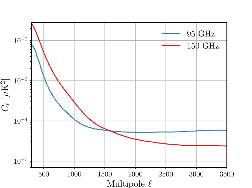
Figure 1: Noise spectra of coadded temperature maps for the 95 and 150 GHz frequency bands.

The noise spectra as a function of multipole, $\ell$, are plotted in Fig. 1. These curves are calibrated and corrected for the transfer function and beam. Compared to 150 GHz, the 95 GHz data has less low-frequency noise from atmospheric fluctuations, but higher noise at $\ell>1600$. The resulting statistical uncertainty for the lensing spectra is similar for 95 and 150 GHz. The white noise levels are 26 $\mu$K-arcmin and 17 $\mu$K-arcmin for 95 and 150 GHz at $\ell\approx 3000$.

II.5 Source Inpainting and Masking

To mitigate the lensing biases from point sources and galaxy clusters, we can remove them in map space using a combination of source inpainting and masking. The inpainting process replaces the pixels around the source with samples drawn from a Gaussian random field with power spectrum consistent with that of the CMB. The samples are constrained to have correlations with the surrounding pixels that follow the predicted CMB correlation function [44]. For source masking, we multiply the map with a mask that effectively zeroes the source pixels using cosine tapers, which smoothly decrease from 1 to 0, following the shape of a cosine curve. Masking holes introduce a mean field that can be estimated using simulations and subtracted from the lensing map (Sec. IV.1). To reduce the mean field and its associated uncertainties, we inpaint most of the sources and mask bright ones that are above $50$ mJy at 150 GHz. Inpainting or masking sources and clusters with our thresholds discussed below corresponds to cutting 4% of the map area.

The inpainting method used here is similar to that used in Benoit-Lévy et al. [45] and Raghunathan et al. [46]. We define two regions around the source or cluster center, $R\leq R_{1}$ and $R_{1}<R\leq R_{2}$, where $R_{1}$ is the inpainting radius and $R_{2}$ is fixed to be 25^′. We fill values within $R_{1}$ based on values in the $R_{1}<R\leq R_{2}$ annulus using constrained Gaussian realizations

$$\hat{T}_{1}=\tilde{T}_{1}+\hat{\bm{C}}_{12}\hat{\bm{C}}_{22}^{-1}(T_{2}-\tilde{T}_{2})\,,$$ (1)

where 1 indicates the $R\leq R_{1}$ region, 2 indicates the $R_{1}<R\leq R_{2}$ region, $T$ is the original map, $\hat{T}$ is the inpainted map, $\tilde{T}$ is the simulated Gaussian map realization, and $\hat{\bm{C}}_{XY}$ is the covariance matrix of the CMB fields between two regions X and Y. We generate Gaussian realizations in a fixed $200^{\prime}\times 200^{\prime}$ box with the same CMB, foreground, noise spectra, and transfer function as the data to be inpainted. We estimate the covariance matrices $\hat{\bm{C}}_{12}$ and $\hat{\bm{C}}_{22}$ with 5000 Gaussian realizations following the method in Raghunathan et al. [46].

We inpaint or mask all sources detected above $S/N$ of 5 in any of the three frequency bands. The $S/N$ threshold roughly corresponds to minimum fluxes of 2.7, 3.3, and 12.0 mJy at 95, 150, and 220 GHz. We set the inpainting radii based on the maximum flux across the three frequency bands for each source. The radii are summarized in Tab. 1. We inpaint all detected sources, including the brighter sources ($>50$ mJy) that will be later zeroed by masking to reduce the impact of their variance in the covariance matrix on neighboring regions to be inpainted. Similarly, we inpaint clusters detected with $S/N$ $>$ 5. The cluster-finding process was performed using two years of SPT-3G data, resulting in a $S/N$ for the detected clusters that is 1.5 times higher compared to the $S/N$ reported for the same clusters in the SPT-SZ survey [47]. Note that this is a preliminary cluster list, and the $S/N$ for a full analysis will be much higher.

Table 1: Inpainting and masking radii.

	Flux ($S$ in mJy) or cluster $S/N$	Inpainting radius	Masking radius
Point sources	$S\leq 6$	$2^{\prime}$	$-$
	$6<S\leq 20$	$3^{\prime}$	$-$
	$20<S\leq 50$	$5^{\prime}$	$-$
	$50<S\leq 500$	$7^{\prime}$	$7^{\prime}$
	$S>500$	$10^{\prime}$	$10^{\prime}$
Galaxy clusters	$5<S/N\leq 9$	$5^{\prime}$	$-$
	$S/N>9$	$6^{\prime}$	$6^{\prime}$

In addition to the source inpainting, we apply a mask that zeros the region around the brightest point sources in the map. The masking radii are set by flux at 150 GHz for point sources and detection $S/N$ for galaxy clusters (see Tab. 1). The source mask has cosine tapers with a radius of $10^{\prime}$. With $\sim$4% of the area lost due to masking and inpainting, we expect the bias from masking locations correlated with the underlying $\phi$ field to be negligible [see, e.g., 48]. The masking thresholds correspond to 361 sources being masked, and the resulting mean field is well-behaved. We show that the analysis is robust to these inpainting and masking choices in Sec. V.3.

Besides source masking, we apply a boundary mask with $30^{\prime}$-cosine taper to downweight the noisy field edges.

II.6 Inverse-variance Filtering

To minimize the variance of the reconstructed lensing map, the weights applied in the quadratic estimator include inverse-variance filtering the input CMB maps (Sec. IV.1). To construct the filter, we model the data maps as consisting of three components: the CMB sky signal, referred to as $T_{\bm{\ell}}$; “sky noise,” $N_{\bm{\ell}}$, which includes astrophysical foregrounds and atmospheric noise; and pixel-domain noise, $n_{j}$, modeled as white, uncorrelated, and spatially non-varying within the mask. We express the relationship between the data maps and the three components as follows:

$$T_{j}=\sum_{\bm{\ell}}P_{j\bm{\ell}}T_{\bm{\ell}}+\sum_{\bm{\ell}}P_{j\bm{\ell}}N_{\bm{\ell}}+n_{j}\,.$$ (2)

Here, the matrix operator $P_{j\bm{\ell}}$ incorporates the transfer function and Fourier transform, enabling the conversion from Fourier space to map space. It is defined as $P_{j\bm{\ell}}=e^{i\bm{\ell}\mathbf{x}_{j}}F_{\bm{\ell}}$, where $F_{\bm{\ell}}$ contains the beam, pixelization effects, and timestream filtering. The position vector $\mathbf{x}_{j}$ represents the coordinates of pixel $j$.

The inverse-variance filtered field $\bar{T}$ is given by:

$$\bar{T}=S^{-1}[S^{-1}+P^{\dagger}n^{-1}P]^{-1}P^{\dagger}n^{-1}T\,,$$ (3)

where the total signal covariance matrix $S=C_{\bm{\ell}}^{TT}+C_{\bm{\ell}}^{NN}$ has contributions from the CMB, foregrounds, and anisotropic noise. $C_{\bm{\ell}}^{TT}$ represents the sum of CMB and foreground spectra interpolated to 2D, while $C_{\bm{\ell}}^{NN}$ corresponds to the 2D anisotropic noise spectrum. The term $n$ denotes the pixel-space noise variance multiplied by the mask.

For $C_{\bm{\ell}}^{TT}$, we use the same CMB and foreground spectra (namely a CMB TT spectrum and extragalactic foreground spectra representing tSZ, kSZ, CIB, and diffuse radio sources) that were used in generating the CMB simulations discussed in Sec. III. To estimate $C_{\bm{\ell}}^{NN}$, we generate 500 noise realizations by subtracting the left-going and right-going CMB maps and adding the difference maps with random signs. We average the noise spectra over these 500 noise realizations and subtract a white noise level $n$, modeled in pixel space, from the averaged 2D noise spectrum for each band. We solve for $\bar{T}$ with a conjugate-gradient solver.

II.7 Fourier Space Masking

In order to mitigate the contamination from instrumental and atmospheric noise at low $\ell$, as well as astrophysical foregrounds dominating over the CMB at high $\ell$, we apply a Fourier mask that includes modes in the multipole range of $\ell$ between 300 and 3000 for the 95 GHz map and between 500 and 3000 for the 150 GHz map. In addition, we apply a cut excluding data with $\ell_{x}<300$ and $\ell_{x}<500$ (referred as $\ell_{\mathrm{xmin}}$ cut hereafter) for the 95 and 150 GHz frequency bands, respectively, to reduce some noisy modes along the scan direction below $\ell_{\mathrm{xmin}}$. We show in Sec. V.3 that our analysis is robust to different cut choices.

III Simulations

We use simulations to estimate the transfer function, the response (normalization) and mean field correction to the lensing map, the lensing spectrum noise biases ($N^{0}_{L}$, $N^{1}_{L}$), and biases to the lensing spectrum from extragalactic foregrounds.

III.1 CMB and Noise Components

We base the simulated CMB skies on a fiducial cosmology from the best fit of Planck 2018 TT,TE,EE+lowE+lensing [49]. We use CAMB [50] to generate CMB and lensing potential angular power spectra from the fiducial cosmology, and HEALPix [51] to synthesize spherical harmonic realizations of the unlensed CMB and lensing potential. We use Lenspix [52] to create lensed CMB realizations. The instrument and sky noise realization generation is described in Sec. II.6.

III.2 Foreground Components

The millimeter-wave sky, while dominated by the CMB at high galactic latitude, also contains signals from the cosmic infrared background (CIB), thermal and kinetic Sunyaev-Zel’dovich effects (tSZ, kSZ), and radio sources. We model the sub-inpainting-threshold/diffuse foreground emissions below 6.4 mJy at 150 GHz as Gaussian described by their measured angular power spectra. The measured foreground spectra are based on Reichardt et al. [53, hereafter R21]. The CIB in the simulation consists of a Poisson-distributed component with $D_{\ell}\propto\ell^{2}$ from faint dusty star-forming galaxies and a clustered part with $D_{\ell}\propto\ell^{0.8}$. Here $D_{\ell}$ is related to angular power spectrum $C_{\ell}$ by $D_{\ell}=\frac{1}{2\pi}\ell(\ell+1)C_{\ell}$. The spectral shape of the CIB is set to be $\nu^{\beta}B_{\nu}(T_{\mathrm{dust}})$, where $B_{\nu}$ is the blackbody spectrum, $T_{\mathrm{dust}}$ is 25 K, and $\beta$ is $1.48$ for the Poisson term and $2.23$ for the clustered term. At 150 GHz and $\ell=3000$, the amplitude of $D_{\ell}^{\mathrm{CIB}}$ is $D_{3000}^{\mathrm{CIB,P}}=7.24\,{\rm\mu K}^{2}$ for the Poisson term and $D_{3000}^{\mathrm{CIB,cl}}=4.03\,{\rm\mu K}^{2}$ for the clustered term. The clustered term includes the contributions from one- and two-halo terms [54]. The shapes of the tSZ and kSZ angular power spectra follow the tSZ template in Shaw et al. [55] and the kSZ template in Shaw et al. [56] and Zahn et al. [57]. The amplitude at 143 GHz and $\ell=3000$ is $D_{3000}^{\mathrm{tSZ}}=3.42\,{\rm\mu K}^{2}$ for tSZ and $D_{3000}^{\mathrm{kSZ}}=3.0\,{\rm\mu K}^{2}$ for kSZ. The radio source component has a spectrum shape of $D_{\ell}\propto\ell^{2}$ and amplitude of $D_{3000}^{\mathrm{radio}}=1.01\,{\rm\mu K}^{2}$ at 150 GHz. The population spectral index of the radio sources is set to be $\nu^{-0.76}$. The tSZ and radio spectra are adjusted from the measured values in R21 given the different masking and inpainting thresholds in this analysis described in Sec. II.5.

We use these Gaussian foreground simulations to account for the contribution of foregrounds to the disconnected bias term ($N^{0}_{L}$) in the lensing spectrum. However, this set of simulations does not account for the non-zero trispectrum and primary and secondary bispectrum biases [58, 59] one expects from these extragalactic foregrounds. We discuss our approach to estimating the foreground biases in Sec. IV.5.

Besides the diffuse foregrounds, the observed maps also contain point sources and galaxy clusters. We identify point sources and galaxy clusters in the data maps using simplified versions of methods in Everett et al. [60] and Bleem et al. [47]. We check that the point source fluxes and the galaxy clusters’ peak amplitudes are unbiased and accurate to within 10% based on previous measurements for overlapping detections. We include point sources and clusters at their detected positions, amplitudes, and profiles in the simulated maps for all three frequencies. We use the beam profile for point sources and a beta profile [61] convolved with the beam for galaxy clusters. The point sources and clusters are the same between data and simulations, which allows us to use the same masks and inpainting for both.

III.3 Simulation Processing and Transfer Function

We convolve the simulated CMB and foreground maps with the corresponding beams of the three frequency bands. We then mock-observe the simulations using the same methods for data processing so that the mock-observed simulations have the same filter transfer function and mode-coupling as the data maps. We also add the noise maps discussed in Sec. II.6 to the mock-observed maps.

The transfer function is obtained as the square root of the ratio of the 2D power spectra of the mock-observed map and the noise-free simulated map. To reduce noise scatter in the estimate, we average and smooth the transfer functions obtained from 160 simulations. We note that the transfer function shows a small dependence on the power spectra of the input maps. Small changes in the transfer function lead to variations in the weighting of the CMB modes at the inverse-variance filtering step (Sec. II.6), affecting the optimality of the filtered map. We show the effect of using different input spectra to estimate the transfer function on the reconstructed lensing spectra to be negligible in Sec. V.3.

III.4 Simulations for Estimating Foreground Biases

While the simulations described so far are needed for pipeline checks and estimating the transfer function (Sec. III.3) and lensing biases (Sec. IV.3), they also assume no other astrophysical sources of statistical anisotropy besides lensing. However, extragalactic foregrounds are non-Gaussian themselves and correlated with the lensing field. Therefore, we expect an extragalactic foreground bias to our measurement. The galactic foregrounds have negligible effects on our lensing reconstruction since our field is chosen to have low galactic foregrounds.

To estimate the foreground bias, we use the AGORA simulation [59], an N-body-based simulation with tSZ, kSZ, CIB, radio sources, and weak lensing components. A CMB map lensed with the $\phi$ field obtained by ray-tracing through the lightcone is combined with appropriately scaled foreground components (that are correlated with $\phi$) to produce mock 95 and 150 GHz maps.

We create a parallel set of simulations with the same CMB field but Gaussian realizations of foregrounds that have identical power spectra to the sum of all non-Gaussian foregrounds. Both the Gaussian and non-Gaussian simulations will later be used to estimate the foreground bias template in Sec. IV.5. We have one full-sky realization of AGORA simulations at 95 and 150 GHz and we cut them into 16 patches the size of our observing field (Fig. 3). The AGORA simulations, along with their Gaussian counterparts, undergo the same inpainting and masking procedure as the data described in Sec. II.5. This ensures that point sources and galaxy clusters have consistent masking thresholds and corresponding radii as the data. The power spectra of the inpainted and masked AGORA non-Gaussian simulations are within 10-20% of the simulations used for the baseline analysis discussed in Sec. III.2.

IV Lensing Analysis

IV.1 Quadratic Lensing Estimator

The unlensed CMB is well described by a statistically isotropic Gaussian random field with zero off-diagonal covariance. Lensing breaks the statistical isotropy and introduces off-diagonal correlations across CMB temperature and polarization modes in harmonic space. In the general case where $X$ and $Y$ $\in[T,E,B]$, the covariance in the flat-sky approximation is

$$\langle X_{\boldsymbol{\ell\phantom{{}^{\prime}}}}Y^{*}_{\boldsymbol{\ell^{\prime}}}\rangle_{\rm CMB}=\delta(\boldsymbol{\ell}-\boldsymbol{\ell}^{\prime})C_{\ell}^{XY}+W^{XY}_{\boldsymbol{\ell},\boldsymbol{\ell^{\prime}}}\phi_{\boldsymbol{\ell}-\boldsymbol{\ell}^{\prime}}+\mathcal{O}(\phi^{2})\,,$$ (4)

where $\bm{\ell}$ ($\bm{\ell}^{\prime}$) is a vector in Fourier space, $\phi$ is the lensing potential, and $C_{\ell}^{XY}$ is the power spectrum of $XY$. For the temperature-based estimator we use in this paper, $W$ is derived as the leading-order coefficient of the CMB correlation in terms of the lensing potential induced by lensing. In this work, we only include temperature, therefore, in the remainder of the paper, we will replace $X$ and $Y$ with $T_{\nu}$ and $T_{\mu}$, the temperature fields at frequencies $\nu,\mu\in[95,150]$ GHz.

Using these off-diagonal correlations, we can estimate the unnormalized lensing potential at $\bm{L}$ by calculating the weighted sum of the inverse-variance filtered lensing modes separated by $\bm{L}=\bm{\ell}-\bm{\ell}^{\prime}$ [62]

$$\bar{\phi}^{T_{\nu}T_{\mu}}_{\bm{L}}=\int{d^{2}\boldsymbol{\ell}W^{TT}_{\boldsymbol{\ell},\boldsymbol{\ell}-\bm{L}}}\bar{T}_{\nu,\boldsymbol{\ell}}\,\bar{T}^{*}_{\mu,\boldsymbol{\ell}-\bm{L}}\,.$$ (5)

Here we use an over-bar to denote an inverse-variance-weighted quantity. $W^{TT}$ in Eq. 5 is designed to maximize the sensitivity to the lensing-induced signal while minimizing noise. For temperature, $W^{TT}$ for lensing reconstruction takes the same form as the correlation coefficient derived from Eq. 4.

In realistic cases, $\bar{\phi}^{T_{\nu}T_{\mu}}_{\bm{L}}$ contains biases from other statistically anisotropic sources unrelated to lensing, such as the map mask and inhomogeneous sky noise. We estimate this map-level bias, which we call the mean field (MF) $\bar{\phi}^{T_{\nu}T_{\mu},{\rm MF}}_{\bm{L}}$, by averaging the lensing estimations of 160 simulations with different realizations of CMB, lensing potential, and noise:

$$\bar{\phi}^{T_{\nu}T_{\mu},{\rm MF}}_{\bm{L}}=\langle\int{d^{2}\boldsymbol{\ell}W^{TT}_{\boldsymbol{\ell},\boldsymbol{\ell}-\bm{L}}}\bar{T}_{\nu,\boldsymbol{\ell}}\,\bar{T}^{*}_{\mu,\boldsymbol{\ell}-\bm{L}}\rangle\,.$$ (6)

The lensing potentials from different simulations are independent and average to zero, so the averaged lensing estimation only contains the MF from common non-lensing features shared among the simulations. We subtract the MF from $\bar{\phi}^{T_{\nu}T_{\mu}}_{\bm{L}}$.

We normalize the mean-field-subtracted lensing potential by the inverse of the response. We obtain the total response by combining an analytic and a Monte-Carlo (MC) response estimate. The analytic response is given by

$$\mathcal{R}^{T_{\nu}T_{\mu},{\rm Analytic}}_{\bm{L}}=\int{d^{2}\boldsymbol{\ell}\,W^{TT}_{\boldsymbol{\ell},\boldsymbol{\ell}-\bm{L}}\times W^{TT}_{\boldsymbol{\ell},\boldsymbol{\ell}-\bm{L}}\mathcal{F}^{T_{\nu}}_{\boldsymbol{\ell}}\mathcal{F}^{T_{\mu}}_{\boldsymbol{\ell}-\bm{L}}}\,.$$ (7)

Here $\mathcal{F}^{T_{\nu}}_{\boldsymbol{\ell}}T_{\nu,\boldsymbol{\ell}}=[C^{T_{\nu}T_{\nu}}_{\boldsymbol{\ell}}+N^{T_{\nu}T_{\nu}}_{\boldsymbol{\ell}}]^{-1}T_{\nu,\boldsymbol{\ell}}$ is an approximation of the inverse-variance filter in Sec. II.6, where the approximation is exact if there is no masking, and $N_{\bm{\ell}}^{T_{\nu}T_{\mu}}$ captures all anisotropic noise. For the general case, we apply an MC response correction $\mathcal{R}_{\bm{L}}^{T_{\nu}T_{\mu},{\rm MC}}$ to account for the deviation from this approximation. We divide the cross-spectrum between the estimated lensing potential and the input lensing potential by the input auto-spectrum and average this ratio over many simulation realizations to get the MC response

$$\mathcal{R}_{\bm{L}}^{T_{\nu}T_{\mu},{\rm MC}}=\frac{\langle\hat{\phi}^{T_{\nu}T_{\mu}}_{\bm{L}}\,\,\phi^{I*}_{\bm{L}}\rangle}{\langle\phi^{I}_{\bm{L}}\phi^{I*}_{\bm{L}}\rangle}\,.$$ (8)

Here $\phi^{I}$ is the input lensing potential and $\hat{\phi}^{T_{\nu}T_{\mu}}_{\bm{L}}$ is the mean-field-subtracted lensing potential with analytic response normalization. We use a hat ($\hat{\phi}$) to denote debiased quantities. We also note that the response is the Fisher matrix for the lensing potential [26, 19], making Eq. 5 an inverse-variance-weighted quantity. We average the MC response into 1D to reduce noise and get $\mathcal{R}_{L}^{T_{\nu}T_{\mu},{\rm MC}}=\langle\mathcal{R}_{\bm{L}}^{T_{\nu}T_{\mu},{\rm MC}}\rangle$. Here $\bm{L}$ is a vector in Fourier space, and $\langle\rangle$ means averaging over an annuli in 2D Fourier space corresponding to the same $L$. The MC response correction $\mathcal{R}_{L}^{T_{\nu}T_{\mu},{\rm MC}}$ is $\lesssim$10% across the range of scales used in this work.

The total response combining the analytic and MC response is $\mathcal{R}_{\bm{L}}^{T_{\nu}T_{\mu}}=\mathcal{R}_{L}^{T_{\nu}T_{\mu},{\rm MC}}\mathcal{R}_{\bm{L}}^{T_{\nu}T_{\mu},{\rm Analytic}}$, and the lensing potential estimate with the full correction is

$$\hat{\phi}^{T_{\nu}T_{\mu}}_{\bm{L}}=\frac{1}{\mathcal{R}^{T_{\nu}T_{\mu}}_{\bm{L}}}(\bar{\phi}^{T_{\nu}T_{\mu}}_{\bm{L}}-\bar{\phi}^{T_{\nu}T_{\mu},{\rm MF}}_{\bm{L}})\,.$$ (9)

IV.2 Lensing Power Spectrum, Biases, and Amplitude

We calculate the lensing power spectrum with the debiased lensing potentials $\hat{\phi}^{T_{\nu}T_{\mu}}$ and $\hat{\phi}^{T_{\alpha}T_{\beta}}$ from different frequency pairs. To account for the border apodization and point source mask applied to the four temperature maps entering the quadratic lensing spectrum estimate, we divide out a masking factor $f_{\rm mask}$, which is the average of the mask applied to a single map to the fourth power, from the spectrum of the debiased lensing potential

$$C^{\hat{\phi}^{T_{\nu}T_{\mu}}\hat{\phi}^{T_{\alpha}T_{\beta}}}_{L}=f_{\rm mask}^{-1}\langle\hat{\phi}^{T_{\nu}T_{\mu}}_{\bm{L}}\,\,\hat{\phi}^{*}\,{}^{T_{\alpha}T_{\beta}}_{\bm{L}}\rangle.$$ (10)

The raw lensing power spectrum is biased by a few sources, including spurious correlations of the input fields to the zeroth and first order of the lensing spectrum, $N^{0}_{L}$ and $N^{1}_{L}$, and the foreground bias to be discussed in Sec. IV.5. There are higher order biases in terms of the lensing spectrum such as the $N^{3/2}$ biases from post-Born corrections and large-scale structure cross-bispectra that are negligible given our noise levels [63]. The debiased lensing spectrum after $N^{0}_{L}$ and $N^{1}_{L}$ correction is

$$\hat{C}^{\phi\phi}_{L}=C^{\hat{\phi}\hat{\phi}}_{L}-N^{\rm RD,0}_{L}-N^{1}_{L}\,,$$ (11)

where $N^{\rm RD,0}_{L}$ is a variant of $N^{0}_{L}$ to be introduced below.

We estimate the $N^{0}_{L}$ and $N^{1}_{L}$ bias terms with simulations. $N^{0}_{L}$ is estimated using

$$N^{0}_{L}= \Big{\langle}C^{\hat{\phi}\hat{\phi}}_{L}[\bar{T}^{\rm MC}_{\nu},\bar{T}^{\rm MC^{\prime}}_{\mu},\bar{T}^{\rm MC}_{\alpha},\bar{T}^{\rm MC^{\prime}}_{\beta}]$$ (12)

$$+ C^{\hat{\phi}\hat{\phi}}_{L}[\bar{T}^{\rm MC}_{\nu},\bar{T}^{\rm MC^{\prime}}_{\mu},\bar{T}^{\rm MC^{\prime}}_{\alpha},\bar{T}^{\rm MC}_{\beta}]\Big{\rangle}_{\rm MC,MC^{\prime}},$$

where $C^{\hat{\phi}\hat{\phi}}_{L}[\bar{T}_{\nu},\bar{T}_{\mu},\bar{T}_{\alpha},\bar{T}_{\beta}]$ denotes the lensing cross-spectrum between two debiased lensing potentials $\hat{\phi}^{T_{\nu}T_{\mu}}$ and $\hat{\phi}^{T_{\alpha}T_{\beta}}$. We use this format instead of Eq. 10 to highlight the superscripts and subscripts when both are present. MC and MC^′ denote simulations with different realizations of the CMB, Gaussian foreground, lensing potential and noise. Applying Wick’s theorem for the contraction in the above equation, only the Gaussian correlations between fields with the same superscript (MC or MC^′) are non-zero. The $N^{0}_{L}$ estimated this way could be inaccurate because the data may have slightly different Gaussian power from the simulations depending on the simulation modeling and realization. To reduce the bias caused by the difference, we adopt a realization-dependent $N^{\rm RD,0}_{L}$ [64] defined by

$$N^{\rm RD,0}_{L}=$$ (13)

$$\Big{\langle} C^{\hat{\phi}\hat{\phi}}_{L}[\bar{T}^{\rm d}_{\nu},\bar{T}^{\rm MC}_{\mu},\bar{T}^{\rm d}_{\alpha},\bar{T}^{\rm MC}_{\beta}]+C^{\hat{\phi}\hat{\phi}}_{L}[\bar{T}^{\rm MC}_{\nu},\bar{T}^{\rm d}_{\mu},\bar{T}_{\alpha}^{\rm d},\bar{T}^{\rm MC}_{\beta}]$$

$$+C^{\hat{\phi}\hat{\phi}}_{L}[\bar{T}^{\rm d}_{\nu},\bar{T}^{\rm MC}_{\mu},\bar{T}^{\rm MC}_{\alpha},\bar{T}^{\rm d}_{\beta}]+C^{\hat{\phi}\hat{\phi}}_{L}[\bar{T}^{\rm MC}_{\nu},\bar{T}^{\rm d}_{\mu},\bar{T}^{\rm MC}_{\alpha},\bar{T}^{\rm d}_{\beta}]$$

$$-N^{0}_{L}\Big{\rangle}_{\rm MC,MC^{\prime}}\,\,\,\,\,,$$

where $d$ denotes the data. In $N^{\rm RD,0}_{L}$, we calculate the lensing spectra from lensing potentials estimated using both the data and simulation. We then subtract $N^{0}_{L}$ bias defined in Eq. 12. This method also suppresses off-diagonal contributions to the covariance of the lensing power spectrum [64].

The $N^{1}_{L}$ bias term arises from connected contributions to the trispectrum and is estimated using simulations with the same lensing field but different CMB realizations. $N^{1}_{L}$ bias is given by

$$N^{1}_{L}=$$ (14)

$$\Big{\langle} C^{\hat{\phi}\hat{\phi}}_{L}[\bar{T}^{\phi^{1},{\rm MC}}_{\nu},\bar{T}^{\phi^{1},{\rm MC^{\prime}}}_{\mu},\bar{T}^{\phi^{1},{\rm MC}}_{\alpha},\bar{T}^{\phi^{1},{\rm MC^{\prime}}}_{\beta}]$$

$$+C^{\hat{\phi}\hat{\phi}}_{L}[\bar{T}^{\phi^{1},{\rm MC}}_{\nu},\bar{T}^{\phi^{1},{\rm MC^{\prime}}}_{\mu},\bar{T}^{\phi^{1},{\rm MC^{\prime}}}_{\alpha},\bar{T}^{\phi^{1},{\rm MC}}_{\beta}]$$

$$-N^{0}_{L}\Big{\rangle}_{{\rm MC,MC^{\prime}}}\,,$$

where $\phi^{1}$ indicates that the simulations share the same lensing field. Here MC and MC^′ indicate that the simulation components other than $\phi$ come from independent realizations. The first two terms contain $N^{0}_{L}$ bias from Gaussian power and the $N^{1}_{L}$ bias from the shared lensing potential among the four subfields. We subtract the $N^{0}_{L}$ bias from the first two terms to get the $N^{1}_{L}$ bias.

We present our results in binned bandpowers. Our bin edges are shown in Table 2. We calculate the weighted average of $\hat{C}^{\phi\phi}_{L}$ within each bin:

$$\hat{C}_{b}^{\phi^{T_{\nu}T_{\mu}}\phi^{T_{\alpha}T_{\beta}}}\equiv\frac{\sum_{{L}\in b}w_{{L}}^{T_{\nu}T_{\mu}T_{\alpha}T_{\beta}}\hat{C}_{{L}}^{\phi^{T_{\nu}T_{\mu}}\phi^{T_{\alpha}T_{\beta}}}}{\sum_{{L}\in b}w_{{L}}^{T_{\nu}T_{\mu}T_{\alpha}T_{\beta}}}.$$ (15)

Here, the subscript $b$ denotes a binned quantity. The weighted average of the $C_{L}$ inputs, denoted as $C_{b}$, is calculated using Wiener-filter weights $w$ designed to maximize our sensitivity to departures from the fiducial $\Lambda$CDM expectation: $w^{T_{\nu}T_{\mu},T_{\alpha}T_{\beta}}_{L}=C^{\phi\phi,{\rm theory}}_{L}/{\rm Var}(\hat{C}^{{\phi}^{T_{\nu}T_{\mu}}{\phi}^{T_{\alpha}T_{\beta}}}_{L})$. We obtain the variance ${\rm Var}(\hat{C}_{L}^{{\phi}{\phi}})$ from analytic estimates of the signal and noise spectrum.

We can then compute the per-bin amplitude, denoted as $A_{b}^{T_{\nu}T_{\mu},T_{\alpha}T_{\beta}}$, which is defined as the ratio of the unbiased lensing spectrum to the input theory spectrum:

$$A_{b}^{T_{\nu}T_{\mu}T_{\alpha}T_{\beta}}\equiv\frac{\hat{C}^{\phi^{T_{\nu}T_{\mu}}\phi^{T_{\alpha}T_{\beta}}}_{b}}{C^{\phi\phi,{\rm theory}}_{b}}\,.$$ (16)

Here ${C^{\phi\phi,{\rm theory}}_{b}}$ is the theory power spectrum in bin $b$ weighted the same way as in Eq. 15.

The overall lensing amplitude for each estimator is calculated in the same manner as the per-bin amplitude in Eq. 16, using the entire range of reported $L$ values.

IV.3 Bias Estimation Using Simulations

To estimate the MF, $N^{0}_{L}$, and $N^{1}_{L}$ bias terms, we generate the following set of Gaussian simulations with inputs as detailed in Sec. III.1 and Sec. III.2:

• A: 500 lensed simulations with foregrounds and noise realizations discussed in Sec. II.6,

• B: 160 lensed simulations with no foregrounds or noise,

• C: 160 lensed simulations with no foregrounds or noise and with the same realizations of lensing potential as set B, but different CMB.

We use all simulations in A to estimate $N^{\rm RD,0}_{L}$ and 340 simulations in A to evaluate the statistical uncertainty of the lensing power spectrum. We use 160 simulations in A to estimate the MF (Sec. IV.1), with 80 sims for each of the two lensing potential estimations that form the lensing spectrum. All of the simulations in set B and C are used to calculate $N^{1}_{L}$, which is proportional to the first order of lensing power and has no contribution from Gaussian foregrounds. The number of simulations used for each estimated term is chosen such that the term estimated converges well below the statistical uncertainty level of the lensing spectrum. In addition to these bias terms, simulations in A are used to estimate the transfer function (Sec. III.3) and the covariance matrix for forming minimum-variance bandpowers (Sec. IV.4). We have performed a pipeline test using Set A to confirm that the reconstructed lensing spectrum is unbiased compared to the input lensing spectrum used to generate the simulations.

We generate a set of 500 unlensed simulations using lensed CMB power spectrum and the same methods for foregrounds as in Set A. We use this set for various diagnostic tests, such as validating the mean lensing spectrum using this set of simulations being consistent with zero for each $L$ bin within a fraction of the statistical uncertainty.

IV.4 Multi-frequency Lensing Spectra Combination

We can reconstruct three individual lensing potential maps from the quadratic combination of the observed temperature fields at the (95, 95), (95, 150), and (150, 150) GHz frequency combinations. By correlating these three $\phi$ maps, we can extract a total of six separate lensing power spectra $C_{L}^{\phi\phi}$.

In this work, we combine the six individual debiased lensing spectra to produce a set of minimum-variance lensing band powers from temperature data. Following previous analyses of primary CMB anisotropies, [e.g., 65, 66, D21], we form a minimum-variance (MV) combination, in the frequency sense, of the lensing band powers $C_{b}$ as

$$C^{\mathrm{MV}}=\left(\mathbb{X}^{\top}\mathbf{\mathbb{C}}^{-1}\mathbb{X}\right)^{-1}\mathbb{X}^{\top}\mathbf{\mathbb{C}}^{-1}C.$$ (17)

Here, $C$ is a vector of length $6N_{\rm bins}$ formed by concatenating the lensing power spectra extracted from the various frequency combinations, while $\mathbb{C}$ denotes their covariance matrix. $\mathbb{X}$ is a design matrix of shape $6N_{\rm bins}\times N_{\rm bins}$ in which each column is equal to 1 in the six elements corresponding to a lensing power spectrum measurement in that $L$-space bin and zero elsewhere. The band power covariance matrix $\mathbb{C}$ used to weight and combine the different lensing reconstructions is estimated with a simulation-based approach, using $N_{\rm sims}=340$ realizations introduced in Sec. III. Given the finite number of simulations, the estimate of the covariance is noisy. To ameliorate the noise of off-diagonal elements, we condition the underlying covariance matrices $\mathbb{C}_{bb^{\prime}}^{\nu\mu\alpha\beta}$ by explicitly setting to zero those entries that we do not expect to be correlated. Specifically, we discard elements that are more than one bin away from the diagonal, i.e. $\mathbb{C}_{bb^{\prime}}^{\nu\mu\alpha\beta}=0$ if $|b-b^{\prime}|>1$. In each $N_{\rm bins}\times N_{\rm bins}$ block of the full covariance matrix $\mathbb{C}_{bb^{\prime}}$, the bins neighboring the diagonal are correlated on average at the 15% level and no more than 30%. Finally, we note that the average correlation coefficient between different lensing reconstructions can be as large as 95% over the $L$ range used in this analysis for two sets of lensing band powers that share three common frequencies, e.g., $\hat{C}^{\phi^{T_{95}T_{95}}\phi^{T_{95}T_{95}}}_{b}$ and $\hat{C}^{\phi^{T_{95}T_{95}}\phi^{T_{95}T_{150}}}_{b}$ and as low as 56% for $\hat{C}^{\phi^{T_{95}T_{95}}\phi^{T_{95}T_{95}}}_{b}$ and $\hat{C}^{\phi^{T_{150}T_{150}}\phi^{T_{150}T_{150}}}_{b}$. We verified that the conditioning applied to the cross-frequency covariance matrices results in a stable estimate of the MV lensing spectrum and its associated covariance matrix. Specifically, we have tested two additional conditioning schemes, one where we only retain the diagonal elements and one based on previous primary CMB SPT analyses [65, 31] where the on- and off-diagonal covariance blocks are treated differently, and found the differences in the recovered MV lensing spectra to be largely subdominant with respect to statistical uncertainties.

IV.5 Astrophysical Foreground Bias Template

We expect the lensing spectrum in Eq. 11 to contain residual biases from extragalactic foregrounds. To address this, we estimate an extragalactic foreground bias template using the simulations described in Sec. III.4. We use this foreground bias template to model the shape of the bias spectrum and marginalize over its amplitude in our lensing amplitude measurement and when estimating cosmological parameters (Sec. VI.1.1).

To compute this template, we difference the lensing spectra extracted using the AGORA simulations with the lensing spectra from Gaussian realizations of foregrounds that have the same power spectra as their non-Gaussian foreground counterparts. The foreground bias template ($\mathcal{T}$) can be expressed schematically as

$$\operatorname{\mathcal{T}}=\hat{C}_{L}^{\phi\phi}\left(\mathrm{CMB}^{\mathrm{NG}}+\mathrm{FG}^{\mathrm{NG}}\right)-\hat{C}_{L}^{\phi\phi}\left(\mathrm{CMB}^{\mathrm{NG}}+\mathrm{FG}^{\mathrm{G}}\right).$$ (18)

Here the superscript NG denotes the non-Gaussian simulations, and G denotes random Gaussian realizations with the same power spectrum. $\mathrm{CMB}^{\mathrm{NG}}$ indicates that the CMB is lensed by large-scale structures correlated with the foregrounds ($\mathrm{FG}^{\mathrm{NG}}$) generated using the same set of N-body simulations. The first term, $\hat{C}_{L}^{\phi\phi}\left(\mathrm{CMB}^{\mathrm{NG}}+\mathrm{FG}^{\mathrm{NG}}\right)$, contains both the trispectrum of the foreground components and the bispectrum with two powers of foreground and one power of the $\phi$ field. The second term contains neither, so their difference is an estimate of the sum of the foreground trispectrum- and bispectrum-type biases. We have applied similar MF, response, and $N^{0}_{L}$ corrections (Eq. 9, 11) described in Sec. IV.2 for both lensing spectra. We do not apply the $N^{1}_{L}$ correction as it differences out in Eq. 18. In addition to Eq. 18, we also estimate the foreground trispectrum and the bispectrum biases separately using $\hat{C}_{L}^{\phi\phi}\left(\mathrm{CMB}^{\mathrm{NG,2}}+\mathrm{FG}^{\mathrm{NG}}\right)-\hat{C}_{L}^{\phi\phi}\left(\mathrm{CMB}^{\mathrm{NG,2}}+\mathrm{FG}^{\mathrm{G}}\right)$ and $\hat{C}_{L}^{\phi\phi}\left(\mathrm{CMB}^{\mathrm{NG}}+\mathrm{FG}^{\mathrm{NG}}\right)-\hat{C}_{L}^{\phi\phi}\left(\mathrm{CMB}^{\mathrm{NG,2}}+\mathrm{FG}^{\mathrm{NG}}\right)$, checking and confirming that their sum is consistent with our template constructed using Eq. 18. Here the superscript 2 indicates that the CMB comes from a different patch such that its lensing field does not correlate with the non-Gaussian foreground or contribute to the bispectrum-type bias.

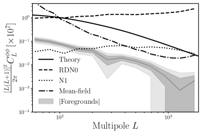
Figure 2: Biases in the CMB lensing auto-spectrum. The solid black line denotes the fiducial CMB lensing power spectrum. The realization dependent $N^{0}_{L}$ and $N^{1}_{L}$ biases for our deepest lensing map, $\hat{\phi}^{T_{95}T_{150}}$ as representative noise levels, are shown in black dashed and dotted lines, respectively. The power spectrum of the mean field (MF) for $\hat{\phi}^{T_{95}T_{150}}$ is plotted in dash-dotted line. The absolute value of the expected mean foreground contamination to the minimum-variance combination (see Sec. IV.4, negative bias) is shown by the solid grey line while the shaded grey areas denote the 1 and 2$\sigma$ scatter with respect to the mean calculated over 16 cutouts from the AGORA simulations.

Fig. 2 shows the foreground bias template to the MV combination (see Sec. IV.4), as well as $N^{\rm RD,0}_{L}$, $N^{1}_{L}$, and MF biases for $\hat{\phi}^{T_{95}T_{150}}$. The 1$\sigma$ and 2$\sigma$ errorbars to the foreground template are estimated from the distribution of 16 bias power spectra estimated using Eq. 18 for the 16 patches discussed in Sec. III.4. We bin the MV foreground bias template using Eq. 15 to get the binned template $C_{b}^{\phi\phi,\rm fg}$. The mean foreground bias amplitude is negative since the bispectrum-type bias is negative at lower $L$ and larger in amplitude than the positive trispectrum-type bias term in the $L$ range shown [59]. The bias amplitude reduces by $\approx$30% as we exclude modes with $\ell>2500$, which is consistent with the foreground power becoming smaller relative to the CMB at lower $\ell$.

As discussed in Sec. IV.4, we combine the multifrequency information in debiased lensing power spectrum space, as opposed to lensing map space. Therefore, in Fig. 2, we show the mean field spectrum, $N^{0}_{L},$ and $N^{1}_{L}$ noise curves for the auto-spectrum of $\hat{\phi}^{T_{95}T_{150}}$, our deepest lensing map, as a representative noise level. The mean field spectrum at low $L$ comes from the boundary mask and converges sufficiently with the number of simulations we used for averaging.

V Lensing Maps, Power Spectra, and Amplitudes

In this section, we present our main results: the lensing convergence map, lensing power spectrum, and lensing amplitude measurements. We discuss the relative weights from independent frequency combinations and compare our results to previous measurements by SPT-SZ (O17), SPTpol (W19), POLARBEAR [24], BICEP/Keck [18], Planck [22], and ACT [3]. We then discuss the lensing amplitude and its statistical and systematic uncertainties.

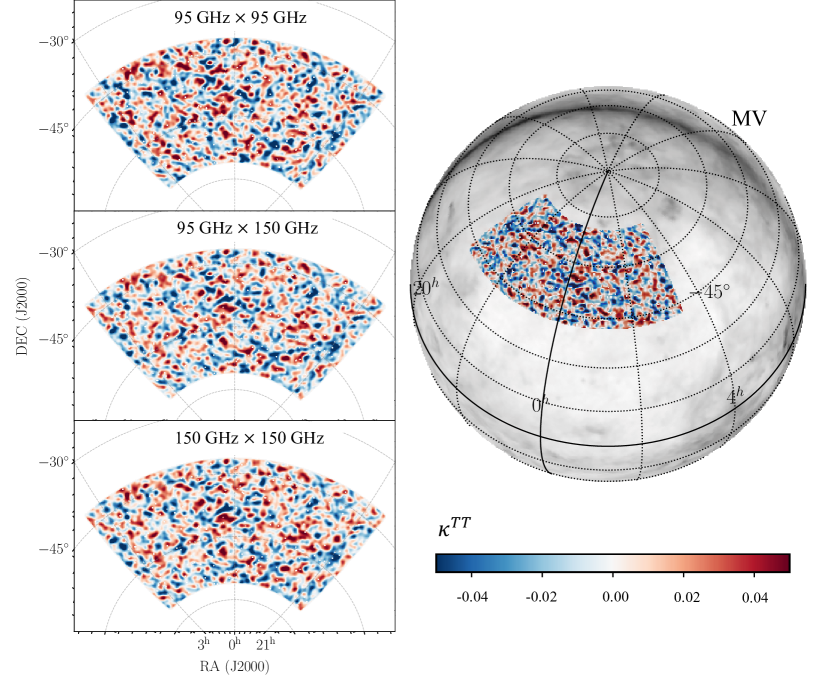
Figure 3: Lensing $\kappa$ maps reconstructed from the SPT-3G 1500 deg² field data, smoothed by a 1-degree FWHM Gaussian to highlight the large-scale modes with higher $S/N$. We have also multiplied the maps by the point source and cluster mask discussed in Sec. II.5. The three left panels show the lensing convergence map inferred from three independent frequency combinations: 95 $\times$ 95 GHz, 95 $\times$ 150 GHz, and 150 $\times$ 150 GHz. The right-hand side shows a minimum-variance-combined CMB lensing convergence map reconstructed in this work using $95$ and $150$ GHz data and projected to Equatorial coordinates. The SPT-3G footprint covers approximately 1500 deg² of the southern sky. The background shows the Galactic dust map from Planck Commander in intensity plotted in a logarithmic color scale.

V.1 Lensing Maps

In Fig. 3, we show the lensing convergence maps $\kappa$ reconstructed from the individual frequency combinations 95 $\times$ 95 GHz, 95 $\times$ 150 GHz, and 150 $\times$ 150 GHz. The convergence is related to the lensing potential $\phi$ as $\kappa=-\frac{1}{2}\nabla^{2}\phi$, which in harmonic space translates to $\kappa_{\bm{L}}=\frac{L(L+1)}{2}\phi_{\bm{L}}$. The $\kappa$ maps in Fig. 3 are smoothed using a 1-degree FWHM Gaussian filter to emphasize the large-scale modes with higher $S/N$. Our lensing maps are signal dominated at lensing multipoles below $L\approx 70,90,100$ for $\hat{\phi}^{T_{95}T_{95}}$, $\hat{\phi}^{T_{150}T_{150}}$, and $\hat{\phi}^{T_{95}T_{150}}$, respectively. The three panels on the left of Fig. 3 have nearly identical structures and are strongly correlated. $\hat{\phi}^{T_{95}T_{95}}$, $\hat{\phi}^{T_{95}T_{150}}$, and $\hat{\phi}^{T_{150}T_{150}}$ share similar $N^{0}_{L}$ noise contributions from Gaussian power of the CMB, thus their MV combination only slightly reduces the uncertainty compared to each individual frequency combination. We include the MV-combined lensing map on the right of Fig. 3, which has almost the same structure as the panels on the left. We show the MV lensing map in Equatorial coordinates to highlight the observing field for this analysis. Our lensing map covers three times the area and has higher reconstruction noise per mode compared to SPTpol (W19). On the other hand, our lensing map is 60% in size and has lower noise per mode compared to SPT-SZ (O17). Our lensing convergence maps show consistent degree-scale structure compared to both the SPTpol and SPT-SZ lensing maps visually.

V.2 Lensing Power Spectra and Amplitude

The lensing band powers from the six individual debiased lensing spectra and their MV combination, defined in Eqs. 16 and 17, are presented in Fig. 4. In addition, we have corrected for the foreground bias contamination estimated in Sec. IV.5 using AGORA simulations that closely match our observing frequencies and map processing steps. The foreground bias template is subject to uncertainties from sample variance and depends on the accuracy of the associated simulations. As a result, we do not directly use these foreground-corrected spectra for cosmological interpretation, but marginalize over the amplitude of the foreground bias template $A_{\rm fg}$ with a conservative uniform prior, as discussed in greater detail in Sec. VI.1.1. We report the lensing power spectra in logarithmically spaced $L$ bins between 50 and 2000. The corresponding MV bandpowers and uncertainties are provided in Tab. 2. The uncertainties of the individual bandpowers and the MV are similar because they are dominated by $N^{0}_{L}$, which is largely shared between lensing map reconstructed from the 95 and 150 GHz input maps. In each multipole bin, the observed lensing power differs no more than $\lesssim 1\sigma$ between different reconstructions. The visual agreement across the spectra recovered from different frequency combinations provides a consistency check and suggests that the foreground biases are not substantially larger in any one combination, though more substantial tests will be done in the next section.

Table 2: MV lensing bandpowers

$[\,L_{\rm min}$	$L_{\rm max}\,]$	$L_{b}$	$10^{7}[L(L+1)]^{2}\hat{C}_{L}^{\phi\phi}/2\pi$
$[\,50$	$67\,]$	$59$	$0.958\pm 0.336$
$[\,68$	$91\,]$	$80$	$1.261\pm 0.233$
$[\,92$	$125\,]$	$109$	$1.061\pm 0.164$
$[\,126$	$170\,]$	$148$	$0.781\pm 0.112$
$[\,171$	$232\,]$	$202$	$0.636\pm 0.081$
$[\,233$	$315\,]$	$274$	$0.442\pm 0.064$
$[\,316$	$429\,]$	$373$	$0.356\pm 0.044$
$[\,430$	$584\,]$	$507$	$0.172\pm 0.029$
$[\,585$	$794\,]$	$690$	$0.084\pm 0.022$
$[\,795$	$1080\,]$	$938$	$0.061\pm 0.018$
$[\,1081$	$1470\,]$	$1276$	$0.059\pm 0.015$
$[\,1471$	$1999\,]$	$1735$	$0.021\pm 0.013$

• MV lensing bandpowers as defined in Eq. 17. Values are for $10^{7}[L(L+1)]^{2}\hat{C}_{L}^{\phi\phi}/2\pi$ given for logarithmically spaced bins between 50 and 2000.

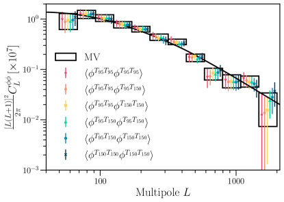
Figure 4: Comparison of the minimum-variance (MV) lensing band powers reconstructed using temperature data at 95 and 150 GHz (black boxes) against band powers from individual frequency combinations (colored points). The solid line is the lensing spectrum from the Planck 2018 best-fit $\Lambda$CDM model.

Table 3: Lensing amplitudes and uncertainties

Freq. comb.	Amp.	Stat. uncert.	Sys. uncert.
$\hat{C}^{\phi^{T_{95}T_{95}}\phi^{T_{95}T_{95}}}_{L}$	1.085	0.073	0.023
$\hat{C}^{\phi^{T_{95}T_{95}}\phi^{T_{95}T_{150}}}_{L}$	1.018	0.063	0.020
$\hat{C}^{\phi^{T_{95}T_{95}}\phi^{T_{150}T_{150}}}_{L}$	1.013	0.060	0.018
$\hat{C}^{\phi^{T_{95}T_{150}}\phi^{T_{95}T_{150}}}_{L}$	1.001	0.061	0.018
$\hat{C}^{\phi^{T_{95}T_{150}}\phi^{T_{150}T_{150}}}_{L}$	0.983	0.062	0.017
$\hat{C}^{\phi^{T_{150}T_{150}}\phi^{T_{150}T_{150}}}_{L}$	1.003	0.066	0.017
MV combined	1.020	0.060	0.016

• Lensing amplitudes for individual frequency combinations and their MV combination. The statistical and systematic uncertainties are also included. The total systematic uncertainties are evaluated by taking the quadrature sum of the individual contributions.

We summarize the lensing amplitudes for each estimator and their MV combination, defined also in Eqs. 16 and 17, in Tab. 3. Similar to the bandpowers, we apply a foreground bias correction assuming the foreground template to be exact. To determine the statistical uncertainties, we utilize the standard deviation of the lensing amplitude distribution based on the 340 simulations within set A discussed in Sec. IV.3. Our lensing amplitude for the MV combination is

$$A^{\rm MV}=1.020\pm 0.060.$$ (19)

Considering solely statistical uncertainty, the lensing amplitude for the MV combination is measured with an uncertainty of 5.9%, which is comparable to the uncertainties of 6.7% using 95 GHz alone and 6.6% for 150 GHz alone. The uncertainty on the amplitude of $\hat{C}^{\phi^{T_{95}T_{95}}\phi^{T_{150}T_{150}}}_{L}$ is the smallest among the six combinations because non-common fluctuations (e.g. instrumental noise) between the 95GHz and 150GHz maps do not contribute to its $N^{0}_{L}$ in this case. We quantify the systematic uncertainties associated with the map calibration factor and beam uncertainty, in Sec. V.4. The systematic uncertainty for the MV combination lensing amplitude is $\pm 0.016$, a fraction of the statistical uncertainties. Considering both statistical and systematic uncertainties, the measurement of the MV lensing amplitude has an uncertainty of 7.5%. In Sec. VI.4.1, we also explore the lensing amplitude using a loose prior on the foreground bias template amplitude $A_{\rm fg}$ and derive a constraint on the lensing amplitude of $A_{L}^{\phi\phi}=1.063\pm 0.090$. This result is consistent with the result reported in Eq. 19.

In Fig. 5, we compare our MV lensing spectra with other experiments. Our measurements agree with previous measurements from SPT-SZ (O17), SPTpol (W19), Planck [22], and ACT [3]. We constrain the lensing amplitude at 5.9%, comparable to SPTpol’s 6.1% (W19) and SPT-SZ’s 6.3% (O17).

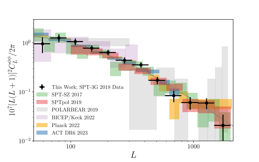
Figure 5: Lensing power spectrum measurements from this work, SPT-SZ (O17), SPTpol (W19), POLARBEAR [24], BICEP/Keck [18], Planck [22], and ACT [3]. We also plot the lensing spectrum from the best-fit $\Lambda$CDM model to the 2018 Planck TT,TE,EE+lowE+lensing dataset (solid gray line) [34, 49].

V.3 Consistency and Null Tests

To ensure the robustness of our analysis and identify potential systematic errors in the data, we conduct a suite of tests. For each test, we modify one aspect of the analysis and recalculate the lensing power spectrum. We then assess the consistency of the results by comparing the bandpower obtained from the modified analysis with that obtained from the baseline analysis. The bandpowers obtained from the different analysis options are summarized in Fig. 6. We designed a suite of tests to specifically check the lensing reconstruction and confirm the pipeline’s robustness against unmodeled nonidealities in the data.

We quantify the $\chi^{2}$ of the tests by comparing the difference data bandpower with the mean of the difference over 340 simulations (Set A in Sec. IV.3), and using the variance of the per-bin simulation-difference spectrum to approximate the covariance diagonal, while neglecting the off-diagonal components, since the difference bandpowers are largely uncorrelated across different bins. The $\chi^{2}$ of the systematic tests are

$$\chi_{\mathrm{sys}}^{2}=\sum_{b}\frac{\left(\Delta\hat{C}_{b,\mathrm{data}}^{\phi\phi}-\left\langle\Delta\hat{C}_{b,\mathrm{sim}}^{\phi\phi}\right\rangle\right)^{2}}{\sigma_{b,\mathrm{sys}}^{2}}.$$ (20)

Here $\left\langle\Delta\hat{C}_{b,\mathrm{sim}}^{\phi\phi}\right\rangle$ and $\sigma_{b,\mathrm{sys}}$ are estimated by performing the same analysis on the 340 simulations as on the data. We compute the differences in overall lensing amplitude $\Delta A_{\mathrm{data}}$ between the alternate analysis choice and the baseline by subtracting the two amplitudes and quantifying the $\chi^{2}$ using the distribution of amplitude differences for the simulations. We also use Eq. 20 to calculate the $\chi^{2}$ values for all our 340 simulations by replacing $\Delta\hat{C}_{b,\mathrm{data}}$ with individual simulation spectra differences. The probability-to-exceed (PTE) is calculated as the fraction of simulation $\chi^{2}$ values that are higher than the $\chi^{2}$ value obtained from the data. We summarize the data $\chi^{2}$ and PTE results in Tab. 4. To account for the look-elsewhere effect using the Bonferroni correction, we stipulate that the PTE values should exceed the threshold of $5\%/N$, with $N=9$ here being the number of tests carried out [67]. Here the different tests are being regarded as independent or weakly dependent. As can be seen in Tab. 4, all our PTE values are above $0.05/9\approx 0.006$. We conclude that we find no signs of significant systematic biases in these tests.

In Fig. 7, we present a visual overview of the consistency tests, illustrating the band power difference relative to the baseline result for each test. The error bars represent the variations derived from the distributions of simulation-difference bandpowers. In each $L$ bin, the data points and error bars are normalized by the 1$\sigma$ lensing spectrum uncertainties in that specific bin. We find that the difference band powers statistically meet expectations with no major systematic shifts for any test. Below, we discuss the results of each consistency test in more detail.

Varying $\ell_{\rm xmin}$, $\ell_{\rm min}$, and $\ell_{\rm max}$: The goals of these tests include checking the reconstruction with different amounts of CMB modes and confirming the robustness of the results against contaminations. Our baseline analysis excludes modes $\ell,\ell_{\mathrm{x}}<300$ at 95 GHz (and $\ell,\ell_{\mathrm{x}}<500$ at 150 GHz) and modes at $\ell>3000$ for both 95 and 150 GHz. We increase $\ell_{\mathrm{min}}$ and $\ell_{\mathrm{xmin}}$ by 200 and reduce $\ell_{\mathrm{max}}$ by 500 compared to the baseline choices. When varying $\ell_{\mathrm{max}}$, we find the lensing spectrum using $\ell_{\mathrm{max}}=2500$ to be consistent with $\ell_{\mathrm{max}}=3000$ at a PTE of 0.09. Also, the cumulative $S/N$ for lensing measurements does not go up significantly beyond $\ell=3000$, so we set this as the high-$\ell$ limit for our baseline analysis. Setting an $\ell_{\mathrm{max}}$ cut also helps reduce the foreground bias, which we estimate in Sec. IV.5. For the lower $\ell$ and $\ell_{x}$ end, we found $\ell_{\mathrm{min}}=\ell_{\mathrm{xmin}}=300$ for 95 GHz (and 500 for 150 GHz) to be an optimal threshold that reduces low-frequency instrumental and atmospheric noise leakage into other $\ell$ ranges (D21) while not removing too many modes. From Tab. 4, the lensing spectra after changing the $\ell_{\mathrm{min}}$ or $\ell_{\mathrm{xmin}}$ are consistent with the baseline with PTEs of 0.30 and 0.24, respectively.

Source Masking and Inpainting: We mask and inpaint extragalactic point sources and galaxy cluster imprints in the CMB map to reduce the bias they contribute (Sec. II.5). We perform several tests to determine whether the masking or inpainting thresholds are sufficient. Note that this is separate from the TOD-level masking discussed in Sec. II.2, which is validated with a separate end-to-end analysis. To explore the impact of masking, we tune the flux threshold of point source masking such that 30% more or 30% fewer sources are masked compared to the baseline. The modified cuts correspond to flux thresholds of 47 mJy and 80 mJy compared to the baseline of 50 mJy at 150 GHz. We also test the impact of inpainting for fainter sources by inpainting 50% fewer sources than the baseline. The modified cuts correspond to source flux thresholds of 6.0, 6.0, and 12.0 mJy at 95, 150, and 220 GHz and cluster detection significance threshold of 9, compared to the baseline choices described in Sec. II.5. The PTEs for bandpower difference relative to the baseline are 0.30 for 30% more masking, 0.03 for 30% less masking, and 0.01 for 50% less inpainting. We note that the data points in Fig. 7 do not move much relative to the baseline results despite the relatively small PTEs for less masking and less inpainting, which indicate that the change in the bandpower is larger than expected from the sims given the same analysis change. Still, the bandpower PTEs are consistent with expected changes from the simulations after we account for the Bonferroni correction. Furthermore, the lensing amplitude PTEs for less masking and less inpainting are 5% and 90%, respectively. We conclude that our results are robust to variations of masking and inpainting choices.

Mask Apodization: Gradients in the masking edges can mimic lensing and be captured by the lensing estimator. The mean field subtraction discussed in Sec. IV.1 should correct for this bias. To check whether the bias from mask apodization is negligible, we change the cosine taper radius for the boundary mask from the baseline of 30^′ to 60^′ and the source mask from 10^′ to 20^′. We repeat the complete analysis process with these changes and find the data difference to agree with the simulation difference distribution with a PTE of 0.37.

Transfer Function Variation: The goal of this test is to confirm our analysis is insensitive to variations in transfer functions estimated using input maps with different power spectra. We test the impact of the transfer function by estimating the transfer functions using another set of Gaussian simulations following a power law spectrum with a spectral index of $-1$ instead of the CMB power spectrum following the method described in Sec. III. The new transfer function has different mode coupling and shifts slightly compared to the baseline transfer function due to a change in the map spectra used to estimate it. We expect the impact to be small because of the response normalization discussed in Sec. IV.1. Using a slightly varied transfer function should only result in a non-optimal weighting and a small degradation of $S/N$. The power spectra using the baseline transfer function and the new one are consistent with a PTE of 0.29.

Curl Test: The lensing deflection field $\bm{d}$ can be decomposed into gradient and curl components: $\bm{d}(\hat{\bm{n}})=\bm{\nabla}\phi(\hat{\bm{n}})+(\star\bm{\nabla})\Omega(\hat{\bm{n}})$, where $\phi$ is the lensing potential, $\Omega$ is the divergence-free or curl component, and $\star$ is a 90^∘ rotation operator [68]. We expect the curl component to be zero at our reconstruction noise levels where higher-order and post-Born effects are negligible [69]. However, foregrounds or other systematic effects may introduce a non-zero curl signal to the data. A curl estimation on the data can test for these signals. The curl spectrum $C_{L}^{\Omega\Omega}$ is extracted using an estimator analogous to the lensing estimator introduced in Sec. IV.1 but designed to respond to the curl component [68]. In addition, there are two key distinctions. First, the theoretical input is set to a flat spectrum $C_{L}^{\Omega\Omega}=10^{-7}$, which is used to uniformly weight the modes when binning, as well as to establish a reference spectrum for the amplitude calculation. Second, no MC response correction from simulations is applied to the reconstructions since the expected signal is zero. Following the method for the lensing spectrum analysis, we correct for other biases to the curl spectrum, including the non-zero $N^{1}_{L}$ bias from the lensing trispectrum [25]. We plot the curl spectrum for the MV combinration in Fig. 6, which is consistent with null at a PTE of 0.18.

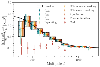
Figure 6: Results of the power spectrum consistency tests and curl null test for the minimum-variance lensing band powers formed by combining temperature data at 95 and 150 GHz. The band powers and errors for the baseline analysis are displayed as boxes. The band powers obtained from the different analysis choices are plotted with different colors and are in agreement with the baseline results. Note that we do not subtract the fiducial foreground bias template from these band powers.

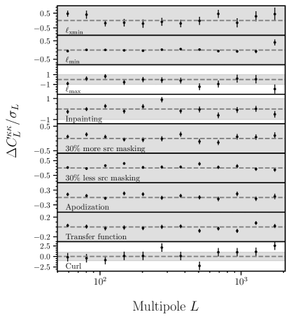
Figure 7: Comparison of difference bandpowers ($\Delta C_{L}^{\kappa\kappa}$) between the baseline analysis and those where we vary a given analysis setting, scaled by the uncertainties of the respective $\phi^{TT}$ bandpowers. The error bars represent the standard deviations of the shifts for 340 simulations with the same analysis choice change. The shaded gray regions represent the 1$\sigma$ bands of the $\phi^{TT}$ estimators.

Table 4: Consistency Tests $\chi^{2}$ and PTEs

Test Name	$\chi^{2}_{\rm MV}$	PTE	$\Delta A_{\rm MV}$	PTE
			$\pm\sigma(\Delta A_{\rm MV})$
$\ell_{\rm xmin}$	15.1	0.24	$-0.017\pm 0.014$	0.32
$\ell_{\rm min}$	13.8	0.30	$\hphantom{-}0.003\pm 0.003$	0.33
$\ell_{\rm max}$	19.1	0.09	$-0.032\pm 0.043$	0.42
Less inpainting	27.7	0.01	$\hphantom{-}0.001\pm 0.012$	0.90
More masking	13.7	0.30	$\hphantom{-}0.004\pm 0.006$	0.50
Less masking	24.6	0.03	$\hphantom{-}0.011\pm 0.006$	0.05
Apod. mask	13.2	0.37	$\hphantom{-}0.001\pm 0.005$	0.28
Transfer func.	14.4	0.29	$-0.002\pm 0.002$	0.54
Curl	16.0	0.18	$-0.038\pm 0.044$	0.40

• Summary of the $\chi^{2}$ for the difference band powers and the difference amplitudes as well as their corresponding PTEs for the systematics tests.

V.4 Systematic Uncertainties

In this subsection, we assess the impact of uncertainties in the beam measurement and temperature calibrations on the lensing amplitude measurement.

Beam uncertainty: To assess the impact of beam-related uncertainties, we introduce perturbations to the baseline beam profile using the uncertainties ($\Delta B_{\ell}$) obtained from D21. These perturbations are applied by multiplying $1+\Delta B_{\ell}$ to the data map while keeping the simulations unchanged. Subsequently, we divide both the data and simulations using the baseline beam, which tests for a systematic 1$\sigma$ underestimation of the beam profile across the entire multipole range. The resulting systematic shift in the amplitude of the lensing power spectrum is $\Delta A_{\rm beam}=0.013$, which is 22% of the statistical uncertainty on $A_{\rm MV}$.

Temperature calibration: We use a temperature calibration factor to calibrate the raw temperature maps via $T=T_{\rm raw}\times T_{\rm cal}$. As outlined in Sec. II.4, we calculate the uncertainty of the calibration factor from Monte-Carlo using simulations with the same noise levels. The uncertainties for the four subfields are similar. By taking their average, the uncertainties associated with $T_{\rm cal}$, $\delta T_{\rm cal}$, are 0.3% and 0.2% for 95 and 150 GHz, respectively. While keeping the simulated maps unchanged, we adjust the data maps by scaling them with ($1+\delta T_{\rm cal}$) for the temperature map, and subsequently re-evaluate the data lensing amplitudes. We then quantify the difference by conducting the baseline analysis with the temperature calibration of the data maps shifted by 1$\sigma$, resulting in a $\Delta A_{\rm cal}=0.010$ for the MV reconstruction, or about $0.16\sigma$ of the statistical uncertainties.

We report the quadrature sum of the beam and temperature calibration uncertainties as the total systematic uncertainty in Tab. 3. The total systematic uncertainty is 0.016, which is smaller than the statistical uncertainty of 0.060. This is smaller than SPTpol’s systematic uncertainty of 0.040 due to the absence of polarization calibration uncertainty, SPTpol’s leading source of systematic uncertainty, in our case. Our systematic uncertainty is similar to that of the temperature-only SPT-SZ measurements.

VI Cosmological parameters

In this section, we present constraints from the 2018 SPT-3G lensing power spectrum on $\Lambda$CDM cosmological parameters as well as on a number of one- and two-parameter extensions. As a reminder, we use the minimum-variance lensing band powers from temperature data introduced in Sec. IV.4 to carry out the cosmological inference.

VI.1 Cosmological Inference Framework

Our baseline cosmology is a $\Lambda$CDM model with a single family of massive neutrinos having a total mass of $\sum m_{\nu}=60$ meV. The model is based on purely adiabatic scalar fluctuations and includes six parameters: the physical density of baryons ($\Omega_{\rm b}h^{2}$), the physical density of cold dark matter ($\Omega_{\rm c}h^{2}$), the (approximated) angular size of the sound horizon at recombination ($\theta_{\rm MC}$), the optical depth at reionization ($\tau$), the amplitude of curvature perturbations at $k=0.05$ Mpc^-1 ($A_{\rm s}$), and spectral index ($n_{\rm s}$) of the power law power spectrum of primordial scalar fluctuations. We also quote constraints derived from these main six parameters, such as $\sigma_{8}$, the square root of the variance of the density field smoothed by a spherical top hat kernel with a radius of 8 Mpc/$h$, as calculated in linear perturbation theory [70], and the Hubble constant $H_{0}$. We then examine a series of $\Lambda$CDM extensions including the sum of the neutrino masses $\sum m_{\rm\nu}$ and the spatial curvature $\Omega_{K}$. The lensed CMB and CMB lensing potential power spectra are calculated with the CAMB Boltzmann code. We sample the posterior space and infer cosmological parameter constraints using the Metropolis-Hastings sampler with adaptive covariance learning provided in the Markov Chain Monte Carlo (MCMC) Cobaya package.

VI.1.1 Lensing Likelihood

The CMB lensing log-likelihood is approximated to be Gaussian in the band powers of the measured lensing power spectrum

$$-2\ln\mathcal{L}_{\phi}(\bm{\Theta})=$$ (21)

$$\qquad\sum_{bb^{\prime}}\left[\hat{C}_{b}^{\phi\phi}-C_{b}^{\phi\phi,\mathrm{th}}(\bm{\Theta})\right]\mathbb{C}_{bb^{\prime}}^{-1}\left[\hat{C}_{b^{\prime}}^{\phi\phi}-C_{b^{\prime}}^{\phi\phi,\mathrm{th}}(\bm{\Theta})\right],$$

where $C_{b}^{\phi\phi,\mathrm{th}}(\bm{\Theta})$ is the binned theory lensing spectrum evaluated at the position $\bm{\Theta}$ in the parameter space, as given by the Boltzmann solver. When combining CMB lensing measurements with primary CMB data, we neglect correlations between the 2- and 4-point functions as these have been shown to not affect the cosmological inference at current noise levels [73, 74, 75, 76]. Therefore, when jointly analyzing CMB lensing and primary CMB, we simply multiply the respective likelihoods. As discussed in Sec. IV.4, the covariance matrix for the minimum-variance lensing binned spectrum is calculated using Monte Carlo simulations from the conditioned covariance matrices. We rescale the inverse covariance matrix by a $\approx 4\%$ Hartlap correction factor [77].

The lensing potential power spectrum estimate depends on cosmology through the response function $\mathcal{R}_{L}$ and on the $N^{1}_{L}$ bias as

$$C_{L}^{\phi\phi,\mathrm{th}}(\bm{\Theta})=\frac{\mathcal{R}_{L}^{2}(\bm{\Theta})}{\mathcal{R}_{L}^{2}(\bm{\Theta}_{\rm fid})}C_{L}^{\phi\phi}({\bm{\Theta}})+N_{L}^{1}(\bm{\Theta})-N_{L}^{1}(\bm{\Theta}_{\rm fid}),$$ (22)

where $\bm{\Theta}_{\rm fid}$ denotes the fiducial cosmology assumed to perform the lensing reconstruction. Here, we follow Planck Collaboration et al. [20], Sherwin et al. [15], Simard et al. [78], Bianchini et al. [2] and take this cosmological dependence into account by linearly perturbing $\mathcal{R}_{L}$ and $N^{1}_{L}$ around $\bm{\Theta}_{\rm fid}$, which amounts to calculating derivatives of the response function with respect to the primary CMB power spectra (in our case only $C_{\ell}^{TT}$) and of the $N^{1}_{L}$ bias with respect to the lensing potential spectrum $C_{L}^{\phi\phi}$. These corrections are computed once for the fiducial cosmology and stored in the matrices $M_{bb^{\prime}}^{TT}$ and $M_{bb^{\prime}}^{\phi\phi}$, respectively. Including the contribution from residual foregrounds, the full prediction for the lensing potential power spectrum takes the following form

$$C_{b}^{\phi\phi,\mathrm{th}}({\bm{\Theta}}) =C_{b}^{\phi\phi}({\bm{\Theta}})+A_{\rm fg}C_{b}^{\phi\phi,\rm fg}$$ (23)

$$+\sum_{x\in\{TT,\phi\phi\}}M^{x}_{bb^{\prime}}\left(C_{b^{\prime}}^{x}(\bm{\Theta})-C_{b^{\prime}}^{x}(\bm{\Theta}_{\rm fid})\right),$$

where summation over $b^{\prime}$ is implied. In Eq. 23, $C_{b}^{\phi\phi,\rm fg}$ is the foreground contamination template introduced in Sec. IV.5 and $A_{\rm fg}$ is the corresponding amplitude parameter on which we impose a uniform prior $A_{\rm fg}\sim\mathcal{U}\left(0,3\right)$. The prior range is motivated by the approximately factor of three difference between the foreground biases estimated from AGORA and from van Engelen et al. [58].

VI.1.2 Cosmological Datasets

In this work, we present parameter constraints obtained from a comprehensive analysis of three main classes of cosmological observables. Our study incorporates the following key observables and survey data:

• CMB lensing: we use the 2018 SPT-3G lensing power spectrum measurement presented in this work along with the lensing bandpowers obtained from the analysis of the Planck CMB PR4 (NPIPE) maps [22]. The SPT-3G and Planck datasets have different sensitivities to different components of the primary CMB due to their limited overlap in the observational footprints (3.6% compared to 67% of the sky), and different noise properties and angular resolution. These two datasets are therefore relatively independent. Additionally, we compare the new constraints from SPT-3G to the previous results from the SPTpol experiment presented in Bianchini et al. [2] and SPT-SZ in Simard et al. [78]. The constraints in Bianchini et al. [2] and Simard et al. [78] are based on the lensing measurements in W19 and O17, respectively.

• BAO: we utilize likelihoods obtained from spectroscopic galaxy surveys, including the BOSS (Baryon Oscillation Spectroscopic Survey) DR12 [79], SDSS MGS [Sloan Digital Sky Survey Main Galaxy Sample; 80], 6dFGS [Six-degree Field Galaxy Survey; 81], and eBOSS DR16 Luminous Red Galaxy [LRG, 82] surveys. Incorporating information about the BAO scale into our analysis allows us to refine the parameter constraints in the $\Omega_{\rm m}$-$H_{0}$ plane and gain insights into the amplitude of the large-scale structure.

• Primary CMB: as our baseline early universe observable, we employ the power spectrum measurements of primary CMB temperature and polarization anisotropies from the Planck 2018 data release [83]. Specifically, we use the low- and high-$\ell$ temperature and polarization likelihoods from PR3 maps. In addition, we make use of the 2018 SPT-3G $TT/TE/EE$ intermediate and small-scale measurements from Balkenhol et al. [33].

Table 5: Cosmological parameters varied in this work and their respective priors. Parameters that are fixed are reported by a single number. $\mathcal{U}(a,b)$ denotes a uniform distribution between $[a,b]$, while $\mathcal{N}(\mu,\sigma^{2})$ indicates a Gaussian distribution with mean $\mu$ and variance $\sigma^{2}$. In addition to these, we include and marginalize over the amplitude of the foreground bias template using a uniform prior $A_{\rm fg}\sim\mathcal{U}(0,3)$. Note that when adding primary CMB information from SPT-3G, we adopt a Planck-based Gaussian prior on $\tau\sim\mathcal{N}(0.0540,0.0074^{2})$.

Parameter	Lensing only (+ BAO)	Lensing + CMB
$\Omega_{\rm b}h^{2}$	$\mathcal{N}(0.02233,0.00036^{2})$	$\mathcal{U}(0.005,0.1)$
$\Omega_{\rm c}h^{2}$	$\mathcal{U}(0.005,0.99)$	$\mathcal{U}(0.001,0.99)$
$H_{0}$ [km/s/Mpc]	$\mathcal{U}(40,100)$	$\mathcal{U}(40,100)$
$\tau$	0.055	$\mathcal{U}(0.01,0.8)$
$n_{\rm s}$	$\mathcal{N}(0.96,0.02^{2})$	$\mathcal{U}(0.8,1.2)$
$\ln(10^{10}A_{\rm s})$	$\mathcal{U}(1.61,3.91)$	$\mathcal{U}(1.61,3.91)$
$\sum m_{\rm\nu}$ [eV]	0.06	0.06 or $\mathcal{U}(0,5)$
$\Omega_{K}$	0	0 or $\mathcal{U}(-0.3,0.3)$
$A_{L}$	1	1 or $\mathcal{U}(0,10)$
$A_{L}^{\phi\phi}$	1	1 or $\mathcal{U}(0,10)$

VI.2 Constraints from CMB Lensing Alone

We start by considering constraints on $\Lambda$CDM parameters from CMB lensing measurements alone, with a special focus on the amplitude of matter fluctuations.

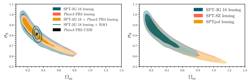
Figure 8: Left: Constraints in the $\Omega_{\rm m}$-$\sigma_{8}$ plane from our SPT-3G CMB lensing measurements (filled blue contours). For comparison, we also include results from Planck PR4 lensing (red contours) as well as its combination with SPT-3G lensing data (yellow contours). The empty blue contours show the constraints combining our SPT-3G lensing likelihood with BAO data. The black filled contours representing the independent constraints derived from the Planck primary CMB power spectra are also found to be consistent with the CMB lensing measurements at lower redshifts. Right: Comparison of $\Omega_{\rm m}$-$\sigma_{8}$ constraints across different SPT surveys.

The parameters that we vary in this analysis and their corresponding priors are listed in Tab. 5. Note in particular that we fix $\tau=0.055$ [34], since CMB lensing is not directly sensitive to the optical depth, and that we impose a Gaussian prior on the baryon density $\Omega_{\rm b}h^{2}=0.02233\pm 0.00036$ based on recent element abundances and nucleosynthesis (BBN) modelling [84, 85] as well as an informative albeit wide prior on $n_{\rm s}$ from Planck CMB anisotropies power spectra [34]. When analyzing SPT-3G CMB lensing measurements without primary CMB power spectra, we fix the linear corrections to the response function to the fiducial cosmology and only vary the ones related to the $N^{1}_{L}$ bias.

Within the base $\Lambda$CDM model, constraints from CMB lensing measurements alone follow a narrow elongated tube in the 3D subspace spanned by $\sigma_{8}$-$H_{0}$-$\Omega_{\rm m}$. This is then projected as an elongated narrow region on the $\Omega_{\rm m}$-$\sigma_{8}$ plane, as shown in Fig. 8. The parameter combination optimally determined by CMB lensing measurements is $\sigma_{8}\Omega_{\rm m}^{0.25}$, which is constrained from SPT-3G data at the $\approx 4.4\%$ level:

$$\sigma_{8}\Omega_{\rm m}^{0.25}=0.595\pm 0.026\quad(\text{{\mbox{\sc SPT-3G}}}).$$ (24)

As a simple and quick way to estimate the agreement between measurements from two (independent) datasets, we calculate the differences in central parameter values normalized to the sum in quadrature of the uncertainties: $(\mu_{1}-\mu_{2})/\sqrt{\sigma_{1}^{2}+\sigma_{2}^{2}}$, where $\mu_{i}$ and $\sigma^{2}_{i}$ are the central values and variances of the two measurements, respectively. With this definition, $\sigma_{8}\Omega_{\rm m}^{0.25}$ inferred from SPT-3G is only $0.13\sigma$ away from the Planck PR4 lensing value of $\sigma_{8}\Omega_{\rm m}^{0.25}=0.599\pm 0.016$ and also in agreement at the 0.5$\sigma$ level with the value of $\sigma_{8}\Omega_{\rm m}^{0.25}=0.609\pm 0.008$ based on the Planck CMB PR3 anisotropies.

In the right panel of Fig. 8, we compare the SPT-3G results with those from the SPT-SZ analysis in O17 and the SPTpol analysis in W19. It is important to note that apart from using three different cameras, these SPT measurements differ in other aspects as well. Firstly, the sky coverage of these measurements are different. Secondly, while this measurement is similar to the temperature-only SPT-SZ analysis in that it relies solely on temperature data, the W19 measurement used both temperature and polarization data, with the latter carrying more statistical weight in the final result. Lastly, the SPT-3G and SPT-SZ lensing power spectra extend to lower multipoles ($L=50$) than the SPTpol measurement ($L=100$). Hence, the SPT-3G and SPT-SZ measurements are more similar in that they both use temperature data and cover a largely overlapping sky area, whereas SPT-3G and SPTpol provide relatively independent assessments of cosmology.

As can be seen from the right panel of Fig. 8, the main difference between the SPT-3G dataset and its predecessors is that the bulk of the posterior mass moves to a region of the parameter space with lower $\Omega_{\rm m}$ and higher $\sigma_{8}$, excluding the high-$\Omega_{\rm m}$ tail present in the SPT-SZ/SPTpol datasets. In particular, SPT-3G prefers a higher primordial scalar spectrum amplitude ($A_{\mathrm{s}}$), a parameter closely related to $\sigma_{8}$, with $\log(10^{10}A_{s})=3.22^{+0.27}_{-0.23}$ than what is preferred by either SPT-SZ, at $2.76^{+0.31}_{-0.28}$, or SPTpol, at $2.65\pm 0.35$. While bandpower fluctuations can lead to higher or lower preferred $\Omega_{\rm m}$ and $\sigma_{8}$ values, neither of which CMB lensing constrains particularly well, the combination $\sigma_{8}\Omega_{\rm m}^{0.25}=0.595\pm 0.026$ from SPT-3G is in good agreement with the values from SPTpol and from SPT-SZ.

We also note that our constraints are robust against details of the foreground treatment. For example, when fixing the amplitude of the foreground contamination template $A_{\rm fg}$ to unity, the inferred constraint on the amplitude of structure becomes $\sigma_{8}\Omega_{\mathrm{m}}^{0.25}=0.589\pm 0.024$, only a 8% reduction in uncertainty and less than $0.25\sigma$ shift in the central value.

We then proceed to combining the SPT-3G and Planck lensing measurements. Given the independence (Sec. VI.1.2) and the consistency of the SPT-3G and Planck measurements, their combination then involves a straightforward multiplication of the lensing likelihoods associated with each dataset. The constraint on $\sigma_{8}\Omega_{\rm m}^{0.25}=0.596\pm 0.014$ is improved by about 13% with respect to Planck lensing-only statistical uncertainties. A summary of the marginalized $\sigma_{8}\Omega_{\rm m}^{0.25}$ constraints across different datasets is provided in Fig. 9 and the numerical values are reported in Tab. 6.

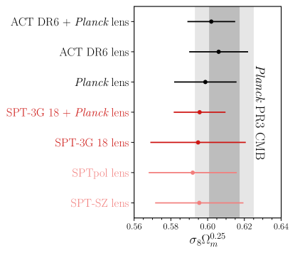
Figure 9: Marginalized $\sigma_{8}\Omega_{\rm m}^{0.25}$ posterior across different SPT, Planck, and ACT CMB lensing measurements. The shaded dark and light grey regions denote respectively the 1 and 2$\sigma$ statistical errors from Planck PR3 CMB temperature and polarization anisotropies.

Table 6: Constraints on a subset of $\Lambda$CDM parameters using the Planck and SPT-3G CMB lensing datasets alone, jointly analyzed, or combined with BAO information. All intervals quoted in this table are 68% intervals, $H_{0}$ is in units of km s^-1Mpc^-1.

	Lensing	Lensing + BAO
	$\sigma_{8}\Omega_{\rm m}^{0.25}$	$\sigma_{8}$	$H_{0}$	$\Omega_{\rm m}$	$S_{8}$
SPT-3G 18	$0.595\pm 0.026$	$0.810\pm 0.033$	$68.8^{+1.3}_{-1.6}$	$0.320^{+0.021}_{-0.026}$	$0.836\pm 0.039$
Planck	$0.599\pm 0.016$	$0.815\pm 0.016$	$68.4\pm 1.1$	$0.313\pm 0.015$	$0.833\pm 0.029$
SPT-3G 18 + Planck	$0.596\pm 0.014$	$0.810\pm 0.014$	$68.1\pm 1.0$	$0.309\pm 0.014$	$0.822\pm 0.024$
SPT-SZ	$0.597\pm 0.024$	$0.789\pm 0.027$	$71.0^{+1.7}_{-2.0}$	$0.361^{+0.028}_{-0.033}$	$0.865\pm 0.041$
SPTpol	$0.592\pm 0.024$	$0.775\pm 0.023$	$71.5^{+1.7}_{-2.1}$	$0.369^{+0.029}_{-0.035}$	$0.858\pm 0.037$

VI.3 Constraints from CMB Lensing and BAO

Next, we turn our attention to the cosmological implications that arise from the inclusion of BAO data with CMB lensing measurements. In addition to providing constraints on $\sigma_{8}$ and $\Omega_{\rm m}$, the CMB lensing power spectrum is sensitive to the expansion rate $H_{0}$ due to its influence on the parameter combination $\sigma_{8}\Omega_{\rm m}^{0.25}(\Omega_{\rm m}h^{2})^{-0.37}$ [20, 87, 72]. Within $\Lambda$CDM, the CMB lensing power spectrum can be written as an integral over the matter power spectrum $P_{\delta\delta}(k,z)$. As a result, $C_{L}^{\phi\phi}$ is sensitive to the broadband shape of $P_{\delta\delta}(k,z)$, which is mostly controlled by the scale of matter-radiation equality $k_{\rm eq}\equiv a_{\rm eq}H_{\rm eq}\propto\Omega_{\rm m}h^{2}$ and the primordial amplitude $A_{s}$. The shape and amplitude of the CMB lensing potential power spectrum are thus sensitive to a degenerate combination of the multipole corresponding to matter-radiation equality scale, $\ell_{\rm eq}\equiv k_{\rm eq}\chi_{*}\propto\Omega_{\rm m}^{0.6}h$, and $A_{\rm s}$ [or $\sigma_{8}$, see, e.g., 86, 20, 2, 72]. The precise extent of the $A_{\rm s}$-$\ell_{\rm eq}$ parameter degeneracy is dictated by how accurately $C_{L}^{\phi\phi}$ is reconstructed and by the range of scales the lensing measurement probes. Therefore, by effectively providing a handle on $\Omega_{\rm m}$, measurements of the projected BAO scale from low-$z$ galaxy surveys can break the $\sigma_{8}$-$\Omega_{\rm m}$-$H_{0}$ degeneracy and sharpen constraints on the individual parameters.

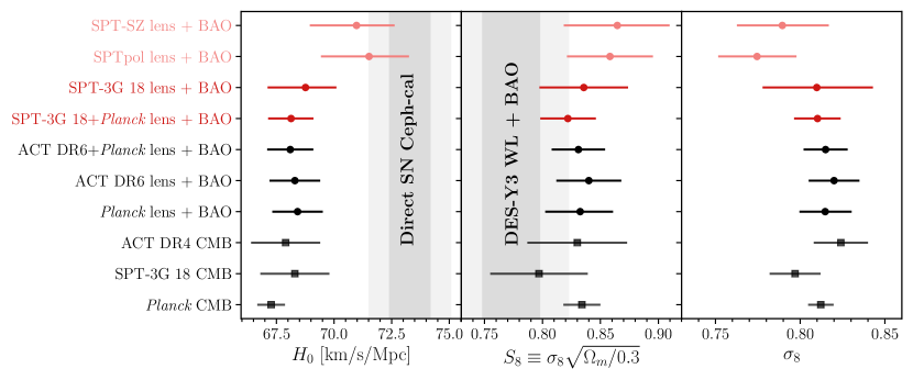
Figure 10: A comparison of the marginalized constraints on the Hubble constant $H_{0}$, $S_{8}\equiv\sigma_{8}\sqrt{\Omega_{\rm m}/0.3}$, and $\sigma_{8}$ (left to right) across different cosmological probes and surveys. The direct $H_{0}$ measurement is taken from Murakami et al. [37], while the LSS-based constraint on $S_{8}$ is taken from the reanalysis of the DES-Y3 (+ BAO) data of [40] presented in Madhavacheril et al. [72].

In Tab. 6, we report constraints from CMB lensing and BAO on $\sigma_{8}$, $\Omega_{\rm m}$, and $H_{0}$. For our baseline SPT-3G measurement, we find the following constraints:

$$\left.\begin{aligned} H_{0}&=68.8^{+1.3}_{-1.6}\,\text{km}\,\text{s}^{-1}\,\text{Mpc}^{-1}\\ \sigma_{8}&=0.810\pm 0.033\\ \Omega_{\rm m}&=0.320^{+0.021}_{-0.026}\end{aligned}\right\}\text{{\mbox{\sc SPT-3G}}{} lensing + BAO.}$$ (25)

The $\sigma_{8}$ and $\Omega_{\rm m}$ parameters are constrained at the $4\%$ and $7\%$ levels, respectively, and are both consistent (central values well within $1\sigma$) with the values inferred by the Planck primary CMB and lensing measurements. The combination of SPT-3G CMB lensing, BAO, and BBN prior yields a $\approx 2\%$ constraint on the expansion rate $H_{0}$ with a central value of 68.8 km s^-1 Mpc^-1. This value is consistent with other CMB lensing- and primary CMB-based constraints of the Hubble constant within the $\Lambda$CDM model (see Fig. 10), as well as the TRGB-calibrated local distance ladder measurement of Freedman et al. [88]. When compared to recent direct $H_{0}$ constraints from Cepheid-calibrated SH0ES supernovae (SN) measurements [37], we find the two estimates to be different at 2.6$\sigma$ significance.

We explore the sensitivity of our results to the low-$L$ bins and foreground marginalization. We compare our baseline result (Eq. 25) to ones without the lowest $L$ bins because the magnitude of the MF bias surpasses that of the signal for scales below $L\lesssim 100$ (see Fig. 2), which might lead one to question the robustness of the baseline result given potential inaccuracies on the MF estimate. When discarding the first two bins of the measured SPT-3G lensing power spectrum (i.e. throwing away information below $L<92$), the parameter constraints become:

$$\left.\begin{array}[]{l}{H_{0}=68.9\pm 1.6}\text{ km s${}^{-1}$ Mpc${}^{-1}$}\\ {\sigma_{8}\,\,=0.809\pm 0.033}\\ {\Omega_{\rm m}=0.322^{+0.027}_{-0.030}}\end{array}\right\}\begin{array}[]{l}{\text{{\mbox{\sc SPT-3G}}{} lensing}}\\ {\text{($L_{\rm min}=92$) + BAO }}.\end{array}$$ (26)

While the uncertainties on some of the parameters slightly deteriorate, the inferred central values are largely unchanged. The parameter that is affected most is $\Omega_{\rm m}$, whose 1$\sigma$ uncertainty is degraded from $0.024\to 0.028$, followed by $\sigma(H_{0})=1.5\to 1.6$. We also find foreground marginalization does not dramatically affect the cosmological inference. We test this by setting $A_{\rm fg}=1$ and repeating the MCMC analysis. The parameter that is affected most by the change is $\sigma_{8}$ for which we find an updated 1$\sigma$ constraint of $\sigma_{8}=0.805^{+0.029}_{-0.026}$. As can be seen, the shift in the central value is 0.15$\sigma$ and the $A_{\rm fg}$ marginalization degrades the sensitivity by about 17%.

The constraints in Eqs. 25 are sharpened when lensing information from Planck PR4 lensing is included:

$$\left.\begin{array}[]{l}{H_{0}=68.1\pm 1.0}\text{ km s${}^{-1}$ Mpc${}^{-1}$}\\ {\sigma_{8}\,\,=0.810\pm 0.014}\\ {\Omega_{\rm m}=0.309\pm 0.014}\end{array}\right\}\begin{array}[]{l}{\text{{\mbox{\sc SPT-3G}}{} lensing }}\\ {\text{+{Planck}{} lensing }}\\ {\text{+ \rm BAO }}.\end{array}$$ (27)

There are several intriguing differences between these results and those from the previous SPTpol and SPT-SZ lensing+BAO analyses. Firstly, as shown in Tab. 6, the precision of constraints on $\Omega_{\rm m}$ and $H_{0}$ obtained from SPT-3G improves by approximately 30% when compared to the corresponding values from SPTpol and SPT-SZ. The $\sigma_{8}$ uncertainties are degraded by $20-30\%$ compared to the other two SPT results, which is shown above to be largely due to foreground marginalization. Secondly, the central values for the $H_{0}$ and $\Omega_{\rm m}$ obtained through SPT-3G lensing shift towards lower values than those from SPTpol and SPT-SZ, while $\sigma_{8}$ increases slightly, mirroring the shifts of $\Omega_{\rm m}$ and $\sigma_{8}$ from lensing-alone constraints in Sec. VI.2. The improvement in the precision of $\Omega_{\rm m}$ and $H_{0}$ is in part explained by the decrease in the $\sigma_{8}$-$H_{0}$-$\Omega_{\rm m}$ posterior volume in SPT-3G compared to SPT-SZ/SPTpol (because of the lower noise in SPT-3G compared to SPT-SZ and the larger area/lower $L_{\rm min}$ compared to SPTpol). The shift to a lower central $H_{0}$ value can be understood as follows. The SPT-3G $\sigma_{8}$-$H_{0}$-$\Omega_{\rm m}$ posterior subspace is shifted to lower $\Omega_{\rm m}$-$H_{0}$ (and higher $A_{\rm s}$ and $\sigma_{8}$) relative to those from SPT-SZ and SPTpol. Intersected by the BAO contours, which are positively correlated in the $\Omega_{\rm m}$-$H_{0}$ plane and favor a high value of $H_{0}=72.7^{+2.2}_{-2.9}$, gives the resulting $\Omega_{\rm m}$-$H_{0}$-$\sigma_{8}$ combinations, with lower $H_{0}$ [e.g. 89]. In other words, the high $H_{0}$ preference from BAO-alone constraints is more effectively pulled down by SPT-3G’s combination of a smaller and shifted posterior subspace. While a thorough analysis of the consistency across the various SPT lensing measurements requires common simulations to properly account for the correlations and is beyond the scope of this work, we note that reasonable shifts in the tilt and amplitude, as well as the magnitude of the uncertainties, within the SPT-3G measurement drive $\lesssim 1\sigma$ shifts in the parameter space. As an example, fixing the amplitude of the foreground template to $A_{\rm fg}=0$ (i.e. neglecting residual foreground contamination in the lensing reconstruction) suppresses the lensing power by about 5% and slightly perturbs the spectrum tilt across the whole $L\in[50,2000]$ range. As a consequence, the corresponding central values of the relevant parameters from SPT-3G move towards the SPT-SZ/SPTpol constraints (but not completely) and become $\Omega_{\rm m}=0.330^{+0.024}_{-0.028}$, $\sigma_{8}=0.783\pm 0.029$, and $H_{0}=69.3^{+1.5}_{-1.6}$.

In order to compare our constraints with the findings from optical weak lensing surveys, we also provide the inference on $S_{8}$, which is defined as $\sigma_{8}\sqrt{\Omega_{\rm m}/0.3}$. This parameter combination is known to be most accurately estimated from galaxy shear measurements and has recently been the subject of intense scrutiny due to $2-3\sigma$ tensions between the primary CMB and galaxy lensing constraints [e.g., 90]. From SPT-3G lensing data in combination with BAO scale information, we find a $4.7\%$ determination of the parameter at the level of

$$S_{8}=0.836\pm 0.039\quad\text{({\mbox{\sc SPT-3G}}{} lensing + BAO)},$$ (28)

or $S_{8}=0.822\pm 0.024$ when jointly analyzed with Planck lensing data. Note that these statistical uncertainties are smaller than the typical errors from current galaxy lensing surveys such as the Dark Energy Survey [DES-Y3, 40, 91, 92], the Hyper Suprime-Cam Subaru Strategic Program [HSC-Y3, 93, 94], and the Kilo Degree Survey [KiDS-1000, 38]. The $S_{8}$ value favored by SPT-3G lensing + BAO is approximately 1.7$\sigma$, 1.6$\sigma$, and 1.8$\sigma$ higher than that from DES, HSC-Y3, and KiDS, respectively. We note that the precision of our $S_{8}$ constraint from CMB lensing and BAO is slightly better than that achieved using primary CMB information from SPT-3G, $S_{8}=0.797\pm 0.042$ [33], with the central value from CMB lensing + BAO being about 0.7$\sigma$ higher.

A visual comparison of the marginalized constraints on the Hubble constant $H_{0}$, $S_{8}$, and $\sigma_{8}$ across different probes and surveys is provided in Fig. 10. We choose two representative values in the literature to highlight direct $H_{0}$ and LSS $S_{8}$ measurements. Our results are in excellent agreement with the ACT DR6 and Planck lensing constraints. For $H_{0}$, we show the result from Murakami et al. [37], $H_{0}=73.29\pm 0.90$, which currently maximizes the tension with the indirect $H_{0}$ Planck-based estimates at the $5.7\sigma$ level, while for the low-$z$ amplitude of structure we pick the galaxy-galaxy lensing and galaxy clustering (the so-called $3\times 2$ pt) measurements from DES-Y3 [40] in combination with BAO data, as presented in Madhavacheril et al. [72]. For completeness, we also point the reader to the recent results from HSC [93, 94], KiDS [38], and the joint analysis of DES and KiDS data [95].

VI.4 Constraints on $\Lambda$CDM extensions

In the following sections, we study the consistency between the amount of lensing favored by direct and indirect lensing measurements, as well as the impact on the sum of the neutrino masses $\sum m_{\rm\nu}$ and curvature density $\Omega_{K}$ constraints when including SPT-3G $C_{L}^{\phi\phi}$ bandpowers in the cosmological inference. We adopt the priors listed in the right column of Tab. 5 and include both the response function and $N^{1}_{L}$ linear corrections to the lensing likelihood, as discussed in Sec. VI.1.1. Note that when replacing Planck primary CMB data with SPT-3G $TT/TE/EE$ measurements from Balkenhol et al. [33], we impose a Planck-based Gaussian prior on the optical depth to reionization of $\tau=0.0540\pm 0.0074$ (which is primarily constrained by a feature in the $TE$ and $EE$ spectra at $\ell<10$).

VI.4.1 Lensing Amplitudes

Lensing imprints in CMB maps can either be reconstructed directly, for example by exploiting the induced higher-order correlations between Fourier modes to measure $C_{L}^{\phi\phi}$ (the main focus of this paper), or indirectly through, e.g., the smearing of the acoustic peaks in the primary CMB spectra. In this section, we compare direct and indirect CMB lensing measurements and ask ourselves two questions: 1) is the amplitude of the reconstructed lensing power spectrum consistent with the fiducial Planck $\Lambda$CDM cosmology and 2) does the amount of lensing preferred by the primary CMB smoothing agree with the one suggested by direct lensing measurement?

We have already partially answered the former question in Sec. V.2, where we have defined a lensing amplitude parameter $A_{L}^{\phi\phi}$ as a weighted rescaling of the measured $\hat{C}_{L}^{\phi\phi}$ with respect to a binned fiducial power spectrum. The lensing amplitudes in Sec. V.2 are directly corrected for the estimated foreground bias template, assuming its amplitude is exact and fixed to $A_{\rm fg}=1$. Here we revisit the lensing amplitude calculation using MCMC by marginalizing over uncertainties in the foreground cleaning. We first fix the lensing power spectrum to the assumed fiducial cosmology, $C_{L}^{\phi\phi}(\bm{\Theta}_{\rm fid})$, and then rescale it by an overall amplitude parameter $C_{L}^{\phi\phi}(\bm{\Theta}_{\rm fid})\to A_{L}^{\phi\phi}C_{L}^{\phi\phi}(\bm{\Theta}_{\rm fid})$. In this run we have two free parameters, $A_{L}^{\phi\phi}$ and $A_{\rm fg}$ (defined in Eq. 23), and we include $N^{1}_{L}$ bias correction in Eq. 23. When using the uniform prior on $A_{\rm fg}\sim\mathcal{U}\left(0,3\right)$, we obtain a lensing power spectrum amplitude normalized to the Planck 2018 TTTEEE+lowE+lensing fiducial cosmology of

$$A_{L}^{\phi\phi}=1.063\pm 0.090,$$ (29)

which is consistent with unity within $\approx 0.7\sigma$. This value is about 4% higher than was found in Sec. V.2 and its associated uncertainty is degraded by a factor of 1.5.

The second question is perhaps more interesting since the amount of lensing determined from the smoothing of the acoustic peaks in the Planck temperature and polarization power spectra is larger, at the $2$ to 3$\sigma$ level, than what is predicted by $\Lambda$CDM and when compared to direct CMB lensing measurements [e.g., 34, 96, 97]. To complicate things further, the magnitude and significance of this anomaly vary between different Planck data releases and likelihood versions [e.g., 98], and ground-based CMB surveys such as SPT and ACT do not observe a similar amount of 2-pt function smearing [99, 33]. To check whether the SPT-3G lensing power spectrum is consistent with the lensing information in the primary CMB 2-point function and with $\Lambda$CDM predictions, we follow Calabrese et al. [100] and Planck Collaboration et al. [34]. In addition to $A_{L}^{\phi\phi}$, we introduce a non-physical parameter $A_{L}$ which scales the lensing power spectrum that affects both the lens reconstruction power and the smoothing of the acoustic peaks.

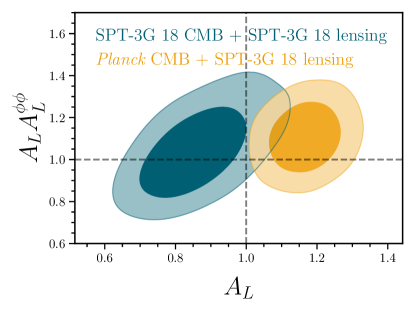
Figure 11: Consistency check between direct and indirect CMB lensing measurements. The amount of lensing directly inferred from SPT-3G data ($A_{L}\times A_{L}^{\phi\phi}$) is consistent with what is predicted by the best-fit $\Lambda$CDM cosmology as determined from primary CMB when the smearing effects ($A_{L}$) are marginalized over. This holds for both Planck PR3 primary CMB (orange contours) as well as 2018 SPT-3G data (blue contours).

In Fig. 11, we show the constraints on the lensing amplitude parameters from the joint analysis of SPT-3G lensing with either Planck or SPT-3G primary CMB anisotropies. In the figure, the combination $A_{L}\times A_{L}^{\phi\phi}$ quantifies the overall amplitude of the measured lensing power with respect to $\Lambda$CDM expectations, when the inferred $\Lambda$CDM parameters have been marginalized over the observed level of peak smearing. As can be seen, while features in the Planck and SPT-3G 2-point CMB spectra drive the preference for either $A_{L}>1$ or $<1$, the amplitude of the lensing power spectrum is consistent with both Planck and SPT-3G primary CMB $\Lambda$CDM predictions when the sensitivity to the peak smoothing effect is artificially removed:

$$A_{L}\times A_{L}^{\phi\phi} =1.11\pm 0.11\,(\text{{Planck}{} CMB + {\mbox{\sc SPT-3G}}{} lens}),$$ (30)

$$A_{L}\times A_{L}^{\phi\phi} =1.04^{+0.13}_{-0.16}\,(\text{{\mbox{\sc SPT-3G}}{} CMB + {\mbox{\sc SPT-3G}}{} lens}).$$

The SPT-3G lensing reconstruction shows no evidence for an unusually high or low amount of lensing relative to that predicted by the best-fit $\Lambda$CDM parameters as determined from primary CMB data when the peak smoothing effect has been marginalized over.

VI.4.2 Neutrino Mass

By being sensitive to matter clustering at intermediate redshifts and mostly linear scales, CMB lensing measurements can also provide insights on the neutrino sector [e.g., 101, 102, 8], one of the most elusive constituents of the standard model of particles. Observations of neutrino flavor oscillations have established that neutrinos are massive particles and that the three known mass-eigenstates are not completely degenerate [103, 104]. However, their absolute mass scale is still unknown. The mass-squared differences measured in oscillation experiments put a lower bound on the sum of the neutrino masses $\sum m_{\rm\nu}>60$ meV, for a normal hierarchy, or greater than 100 meV, for the inverted hierarchy. While tritium beta decay end-point experiments like KATRIN have put constraints on the effective electron anti-neutrino mass at the level of $\sum m_{\rm\nu}<800$ meV [90% C.L., 105], and are expected to improve by a factor of four, cosmological measurements already have a stronger (albeit model dependent) sensitivity and have the potential to make a mass measurement in the next decade or so [34, 106, 107]. In particular, neutrinos become non-relativistic at low redshifts and contribute to both the matter density parameter and the expansion rate but not to the matter clustering on scales below their free-streaming length. Consequently, in a universe where neutrinos possess mass, the growth of structures below the free-streaming length will be suppressed compared to a universe where neutrinos are massless.

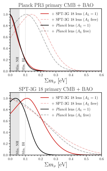
Figure 12: Marginalized constraints on the sum of the neutrino masses $\sum m_{\rm\nu}$ when BAO and either Planck (upper panel) or SPT-3G (lower panel) CMB temperature and polarization power spectra are folded into the cosmological inference. In each panel, the red and black lines show the effect of including direct lensing measurements from SPT-3G and Planck, respectively. The corresponding light dashed lines show instead the constraint when we remove the lensing information in the primary CMB, i.e. we allow $A_{L}$ to vary. The expectations for minimal masses based on oscillation measurements in the normal (NH) and inverted (IH) hierarchies are denoted by the grey shaded band and the dotted vertical line, respectively.

In Fig. 12, we show the marginalized posterior on the sum of the neutrino masses in a $\Lambda$CDM + $\sum m_{\rm\nu}$ cosmology when combining primary CMB, BAO, and CMB lensing datasets (solid lines). When freeing $\sum m_{\rm\nu}$, we follow the argument of Lesgourgues & Pastor [6] and consider a degenerate combination of three equally massive neutrinos, as was done in the Planck papers [34]. The top panel shows the inclusion of Planck primary CMB data, while the bottom one shows the constraints obtained using SPT-3G CMB temperature and polarization spectra as our early universe probe. In each panel, the red and black lines denote respectively the addition of either SPT-3G or Planck lensing datasets. In addition, we also show the corresponding constraints in a $\Lambda$CDM + $\sum m_{\rm\nu}+A_{L}$ cosmology, i.e. when we marginalize over the lensing information in the primary CMB (semi-transparent dashed lines, same color coding as above).

The 95% C.L. constraint on the sum of the neutrino masses from Planck CMB + BAO is $\sum m_{\rm\nu}<0.13$ eV, which remains

$$\begin{split}&\sum m_{\rm\nu}<0.13\,\text{eV}\\ &\quad(\text{{Planck}{} CMB + BAO + {\mbox{\sc SPT-3G}}{} lens},\,2\sigma),\end{split}$$ (31)

when SPT-3G lensing information is added. This constraint with SPT-3G lensing is similar to that with Planck lensing at $\sum m_{\rm\nu}<0.11$ eV. While the inclusion of CMB lensing does not seem to improve or change the constraint significantly, we recall that the neutrino constraints based on Planck PR3 primary CMB are known to be artificially tight because of the anomalous lensing smoothing amplitude (see Sec. VI.4.1). We therefore repeat the exercise when allowing $A_{L}$ to vary. As expected, the $2\sigma$ upper limits combined with SPT-3G and Planck lensing are relaxed to $\sum m_{\rm\nu}<0.32$ eV and $\sum m_{\rm\nu}<0.28$ eV, respectively. In both cases, the posteriors peak at neutrino masses around $\sum m_{\rm\nu}$ around $0.1-0.2$ eV.

To investigate the neutrino constraint sensitivity to primary CMB and potential lensing anomalies, we replace Planck PR3 primary CMB with the latest SPT-3G temperature and polarization power spectra. Although not as constraining as the Planck dataset, SPT-3G can provide a useful consistency check. A joint analysis of SPT-3G CMB + BAO reveals a 2$\sigma$ constraint on the neutrino mass of $\sum m_{\rm\nu}<0.43$ eV, which becomes

$$\begin{split}&\sum m_{\rm\nu}<0.30\,\text{eV}\quad\\ &(\text{{\mbox{\sc SPT-3G}}{} CMB + BAO + {\mbox{\sc SPT-3G}}{} lens},\,2\sigma),\end{split}$$ (32)

with the inclusion of SPT-3G lensing. The corresponding constraint using Planck lensing is comparatively tighter, $\sum m_{\rm\nu}<0.17$ eV. Both posteriors peak at values $\sum m_{\rm\nu}>0$. The lensing parameter $A_{L}$ from SPT-3G primary CMB is about 1$\sigma$ low with respect to $\Lambda$CDM expectations (see Fig. 11). When $A_{L}$ is allowed to vary, the posteriors peak at zero mass and broaden so that the constraints become $\sum m_{\rm\nu}<0.45$ eV (for SPT-3G lensing) and $\sum m_{\rm\nu}<0.32$ eV (for Planck lensing).

VI.4.3 Curvature

CMB lensing measurements also allow us to test the mean spatial curvature of the universe, which is predicted to be close to flat in the majority of inflationary models. Curvature constraints from primary CMB spectra are largely driven by the lensing smoothing on the acoustic peaks, which partially breaks the geometrical degeneracy [108]. Therefore, a direct measurement of the lensing amplitude can further resolve the degeneracy and sharpen constraints on $\Omega_{K}$. Once again, Planck temperature and polarization anisotropies alone present us with a curious feature, showing a $2-3\sigma$ preference for non-flat models [e.g., 34, 109, 110]. This is driven by the $A_{L}$-$\Omega_{K}$ degeneracy and the presence of an enhanced lensing amplitude in the Planck 2018 data release. The preference for a negative curvature weakens in the analysis of Planck NPIPE maps [98] and is not present in either SPT [32] or ACT data [99]. Moreover, the addition of BAO data strongly breaks the geometric degeneracy and eliminates the preference for non-zero $\Omega_{K}$.

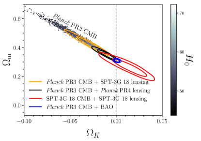
Figure 13: Constraints on curvature and the matter density parameter obtained from the analysis of Planck primary CMB, with scattered points color-coded according to their corresponding Hubble constant values. The orange and black solid lines show the constraints inferred by adding either the SPT-3G or Planck lensing datasets, respectively. The blue solid lines denote instead the constraints from Planck primary CMB combined with BAO data, and indicate consistency with a flat geometry. The constraints obtained from both 2018 SPT-3G primary CMB and lensing are highlighted in red.

The geometrical degeneracy is clearly visible in the colored scatter points in Fig. 13, which show the allowed region in the $\Omega_{K}$-$\Omega_{\rm m}$ parameter space using only primary CMB information from Planck, for which we find $-0.078<\Omega_{K}<-0.010$ (95% C.L.). The inclusion of lensing information from SPT-3G shrinks the allowed 2$\sigma$ region to

$$\Omega_{K}=-0.026^{+0.022}_{-0.024}\,(\text{{Planck}{} CMB + {\mbox{\sc SPT-3G}}{} lens},\,2\sigma),$$ (33)

which is still $\approx 2\sigma$ away from $\Omega_{K}=0$. For comparison, when we instead include Planck lensing, the 2$\sigma$ constraint becomes $\Omega_{K}=-0.011^{+0.012}_{-0.012}$. Using only SPT data for both primary CMB and lensing, the curvature is constrained to

$$\Omega_{K}=0.014^{+0.023}_{-0.026}\,(\text{{\mbox{\sc SPT-3G}}{} CMB + {\mbox{\sc SPT-3G}}{} lens},\,2\sigma),$$ (34)

consistent with a flat universe. Finally, we can turn the limit on the spatial curvature into a constraint on the cosmological constant density parameter $\Omega_{\Lambda}=1-\Omega_{\rm m}-\Omega_{K}$ as done in the first indirect evidence for dark energy using only CMB data [9]. Combining SPT-3G CMB lensing with either Planck or SPT-3G primary CMB, we obtain the following $1\sigma$ bounds:

$$\Omega_{\Lambda} =0.613^{+0.035}_{-0.029}\,(\text{{Planck}{} CMB + {\mbox{\sc SPT-3G}}{} lens}),$$ (35)

$$\Omega_{\Lambda} =0.722^{+0.031}_{-0.026}\,(\text{{\mbox{\sc SPT-3G}}{}\,CMB + {\mbox{\sc SPT-3G}}{}\,lens}).$$

Again, the constraint from Planck CMB and SPT-3G CMB lensing is shifted due to the anomalous peak smoothing in Planck.

VII Conclusions

We have presented the first analysis of CMB lensing using data from SPT-3G, the current camera on the South Pole Telescope. With the 95 and 150 GHz temperature data from the SPT-3G 2018 data set, we produced high-fidelity convergence mass maps over 1500 deg² of the Southern sky, with $S/N$ per mode greater than unity for modes at $L\lesssim 70$ to 100 depending on the frequency combination. We combined the cross-frequency convergence maps and reported a minimum-variance CMB lensing power spectrum over the multipole range $50\leq L\leq 2000$. We constrained the lensing amplitude to be $A^{\rm MV}=1.020\pm 0.060$, a $5.9\%$ precision measurement. The systematic uncertainty, stemming from beam and map calibration uncertainties, is $\pm 0.016$, about 27% of the statistical uncertainty. When marginalizing over a foreground bias template, we found $A^{\phi\phi}_{L}=1.063\pm 0.090$. We conducted a set of consistency checks and null tests on our results and found no evidence of significant bias in our measurement.

We have discussed the cosmological implications of the SPT-3G 2018 data lensing measurements within the $\Lambda$CDM model and in a number of 1- and 2-parameter extensions. Our lensing amplitude agrees with those from ACT and Planck with or without foreground marginalization. While foreground marginalization has minimal impact on cosmological constraints—foreground bias is small compared to the uncertainty—it is included for all cosmological parameter constraints. With SPT-3G 2018 lensing alone, we constrained $\sigma_{8}\Omega_{\rm m}^{0.25}$ to be $0.595\pm 0.026$—a precision of 4.4%. This result is broadly consistent with other CMB lensing measurements, including previous SPT-SZ, SPTpol, ACT, and Planck results, as well as with Planck’s primary CMB anisotropy measurements. When complementing this with BAO data from galaxy surveys, we were able to constrain the matter density and structure amplitude parameters to $\Omega_{\rm m}=0.320^{+0.021}_{-0.026}$ and $\sigma_{8}=0.810\pm 0.033$, consistent with $\Lambda$CDM expectations based on Planck primary CMB. There is some tension between CMB and low redshift measurements of $H_{0}$ and $S_{8}$. When combined with BAO, our measurement is consistent with the cosmology inferred from Planck primary CMB measurements. Specifically, the parameter combination $S_{8}=\sigma_{8}\sqrt{\Omega_{\rm m}/0.3}$ was determined to be $0.836\pm 0.039$, about $1.6-1.8\sigma$ higher than the values inferred from optical surveys such as DES, HSC, and KiDS. The Hubble constant result of $H_{0}=68.8^{+1.3}_{-1.6}$ km s^-1 Mpc^-1 agrees with other early-universe estimates and is approximately $2.6\sigma$ lower than estimates based on Cepheid-calibrated local distance ladder measurements.

The degree of peak smoothing in the temperature power spectrum of Planck, which is 2-3$\sigma$ higher than what is expected from the $\Lambda$CDM model, has notable effects on estimates for cosmological parameters like $\Sigma m_{\rm\nu}$ and $\Omega_{K}$. To isolate the impact from the excess smoothing, we either marginalized over $A_{L}$ when combining with Planck’s primary spectrum or combined with primary spectrum measurements from the SPT-3G 2018 data. First, we demonstrated that SPT-3G 2018 lensing amplitude is consistent with the $\Lambda$CDM expectation when effects of peak smoothing of either Planck or SPT-3G 2018 primary CMB were marginalized over. In combination with the Planck and BAO datasets, the sum of neutrino masses is $\Sigma m_{\rm\nu}<0.13$ eV and $\Sigma m_{\rm\nu}<0.32$ eV (95% C.L) without and with $A_{L}$ marginalized over. Alternatively, when using SPT-3G 2018 CMB data in place of Planck, we obtained $\Sigma m_{\rm\nu}<0.30$ eV (95% C. L.; $A_{L}$=1). Using primary CMB from Planck in combination with SPT-3G lensing drives a $2\sigma$ preference for a non-flat universe and favors a lower $\Omega_{\rm\Lambda}$ of $0.613^{+0.059}_{-0.067}$. The $2\sigma$ preference disappears when replacing the primary CMB from Planck with that from SPT-3G 2018 data, yielding $\Omega_{K}=0.014^{+0.023}_{-0.026}$ (95% C. L.) and $\Omega_{\rm\Lambda}$ of $0.722^{+0.054}_{-0.059}$.

While data for this analysis comes from only half of the 2018 observing season with a half-functioning focal plane resulting in higher per-year map noise, map depths using data from subsequent observing seasons are matching expectations [42]. Our lensing measurement is signal dominated up to $L\simeq 100$; upcoming analyses using two years of data on the 1500 deg² field will expand the signal-dominated region out to multipoles of a few hundred, resulting in a $\approx$2% measurement of the lensing amplitude. At these low map noise levels, polarization measurements will contribute the majority of $S/N$ in future SPT-3G lensing analyses, and employing optimal methods [e.g., 111, 112, 113] will further this dataset’s science reach. High-fidelity lensing maps generated by SPT-3G will be critical in removing the lensing contamination in the search of primordial gravitational waves, parametrized by the tensor-to-scalar ratio $r$, when jointly analyzed with data from BICEP Array [114]. The most stringent constraint on $r$ to date from [115] is already limited by lensing. With SPT-3G’s full-survey lensing map, we expect to improve BICEP Array’s $r$ uncertainty by a factor of about 2.5, reaching $\sigma(r)$ of about 0.003.