Theory of Transverse Mode Instability in Fiber Amplifiers
with Multimode Excitations

Abstract

Transverse Mode Instability (TMI) which results from dynamic nonlinear thermo-optical scattering is the primary limitation to power scaling in high-power fiber lasers and amplifiers. It has been proposed that TMI can be suppressed by exciting multiple modes in a highly multimode fiber. We derive a semi-analytic frequency-domain theory of the threshold for the onset of TMI under arbitrary multimode input excitation for general fiber geometries. We show that TMI results from exponential growth of noise in all the modes at downshifted frequencies due to the thermo-optical coupling. The noise growth rate in each mode is given by the sum of signal powers in various modes weighted by pairwise thermo-optical coupling coefficients. We calculate thermo-optical coupling coefficients for all $\sim$$10^{4}$ pairs of modes in a standard circular multimode fiber and show that modes with large transverse spatial frequency mismatch are weakly coupled resulting in a banded coupling matrix. This short-range behavior is due to the diffusive nature of the heat propagation which mediates the coupling and leads to a lower noise growth rate upon multimode excitation compared to single mode, resulting in significant TMI suppression. We find that the TMI threshold increases linearly with the number of modes that are excited, leading to more than an order of magnitude increase in the TMI threshold in a 82-mode fiber amplifier. Using our theory, we also calculate TMI threshold in fibers with non-circular geometries upon multimode excitation and show the linear scaling of TMI threshold to be a universal property of different fibers.

I Introduction

Fiber lasers based on multi-stage fiber amplifiers (FA) provide an efficient and compact platform to generate ultra-high laser powerEven and Pureur (2002); Jeong et al. (2004); Nilsson and Payne (2011); Jauregui, Limpert, and Tünnermann (2013); Zervas and Codemard (2013); Dong and Samson (2016). This has enabled potential applications in a wide range of technologies such as laser weldingKawahito et al. (2018), gravitational wave detectionBuikema et al. (2019), and directed energyLudewigt et al. (2019). To realize fully this potential, further power scaling is needed in the FAsDawson et al. (2008), which has been limited primarily by nonlinear effects such as transverse mode instability (TMI)Jauregui, Stihler, and Limpert (2020); Eidam et al. (2011a); Smith and Smith (2011); Ward, Robin, and Dajani (2012) and stimulated Brillouin scattering (SBS)Boyd (2020); Kobyakov, Sauer, and Chowdhury (2010); Wolff et al. (2021). TMI is a dynamic transfer of power between the transverse modes of the fiber caused by thermo-optical scatteringHansen et al. (2013); Dong (2013); Ward (2013, 2016); Zervas (2019). During the optical amplification process, heat is generated due to the quantum defect, in an amount proportional to the local optical intensity, creating local temperature fluctuations. The local temperature variations then create refractive index variations, causing significant scattering between the modes. Consequently, when the FA is operated above a certain output power, defined as the TMI threshold, a significant degradation of beam quality occursJauregui et al. (2011, 2012); Otto et al. (2012); Naderi et al. (2013); Kuznetsov et al. (2014); Kong et al. (2016); Stihler et al. (2018, 2020); Menyuk et al. (2021); Chu et al. (2021); Ren et al. (2022), rendering the output unsuitable for many applications. As a result, suppressing TMI or equivalently raising the TMI threshold has been one of the most important and technologically relevant scientific goals in the high-power laser communityZervas and Codemard (2013); Jauregui, Stihler, and Limpert (2020); Jauregui, Limpert, and Tünnermann (2013).

Significant efforts have been undertaken to mitigate TMI, such as dynamic seed modulationOtto et al. (2013), synthesizing materials with low thermo-optic coefficientHawkins et al. (2021); Dong, Ballato, and Kolis (2023), modulating the pump beamTao et al. (2015a); Jauregui et al. (2018), increasing the optical loss of Higher Order Modes (HOMs)Stutzki et al. (2011); Eidam et al. (2011b); Jauregui et al. (2013); Robin, Dajani, and Pulford (2014); Haarlammert et al. (2015); Tao et al. (2016), and utilizing multicore fibersOtto et al. (2014); Klenke et al. (2022); Abedin et al. (2012). Although, most of these efforts have had some success, they suffer from one or more drawbacks, such as fluctuating output power in the case of seed or pump modulation, difficulty with mass-manufacturing custom fibers, and increased guidance of HOMs due to fiber heating, rendering the HOM suppression unfeasible. As such, efficient TMI suppression remains a highly active area of research.

A common feature in all of the previous approaches is to excite the fundamental mode (FM) of the fiber as much as possible, hence reducing the excitation and amplification of HOMsStutzki et al. (2011); Eidam et al. (2011b); Hansen et al. (2011); Jauregui et al. (2013); Robin, Dajani, and Pulford (2014); Haarlammert et al. (2015); Tao et al. (2016); Otto et al. (2014); Klenke et al. (2022); Tao et al. (2015a); Jauregui et al. (2018); Hawkins et al. (2021); Dong, Ballato, and Kolis (2023); Otto et al. (2013). This is motivated by the widespread impression that the speckled internal field generated by multimode excitation will necessarily create a poor beam quality at the outputZhan et al. (2009); Chu et al. (2019). However, recent progress in wavefront shaping, enabled by spatial light modulators (SLM), has demonstrated that multimode excitation with a narrowband seed laser does not inherently lower the beam quality as long as the light remains spatially coherentFlorentin et al. (2017); Geng et al. (2021); Leite et al. (2018). In fact, by using an SLM at either the input or the output end of the fiber, it is possible to obtain a diffraction-limited spot after coherent multimode propagation in both passiveGomes et al. (2022) and active fibersFlorentin et al. (2017), which can be easily collimated using a lens. This enables a fundamentally novel approach to control nonlinear effects in fibers by utilizing selective multimode excitationTeğin et al. (2020); Wright, Christodoulides, and Wise (2015); Krupa et al. (2019); Qiu et al. (2023). The viability of such an approach has recently been demonstrated for other nonlinear effects in fibers such as SBSWisal et al. (2022, 2023); Chen et al. (2023a) and stimulated Raman scattering (SRS)Tzang et al. (2018).

The current authors recently showed, using numerical simulations along with some initial theoretical results, that sending power in multiple fiber modes robustly raises the TMI thresholdChen et al. (2023b). To investigate this approach thoroughly and in detail, we have developed a theory of TMI for arbitrary multimode input excitations and general fiber geometries, building on significant prior theoretical efforts to model TMI, which have been successful in capturing much of the key physicsWard, Robin, and Dajani (2012); Smith and Smith (2013a); Hansen et al. (2013); Dong (2013); Smith and Smith (2013b); Naderi et al. (2013); Hansen, Rymann, and Lægsgaard (2014); Tao et al. (2015b); Jauregui et al. (2015); Zervas (2017); Tao, Wang, and Zhou (2018); Zervas (2019); Menyuk et al. (2021); Dong (2022). It has been shown that TMI can be modelled as exponential growth of noise in the HOMs due to the thermo-optical scattering of the signal. However, as noted, almost all of the previous efforts have focused on the case when only the FM of the fiber is excited with presence of noise in a few HOMs. None of these works attempted to model highly multimode excitations, and their formalisms were not suited for such explorations. As mentioned, some key theoretical results for TMI threshold upon multimode excitation were presented in in ref. Chen et al. (2023b) by the authors of this paper, including results demonstrating linear scaling of the TMI threshold with the number of excited modes. This previous work focused on time-domain numerical simulations, and the detailed theoretical formalism for TMI threshold along with analysis for fibers with arbitrary geometries and input excitations was deferred to the current work.

Here we develop a general formalism that allows efficient calculation of the TMI threshold for arbitrary multimode input excitations and fiber geometries. We derive coupled amplitude equations starting from coupled optical propagation and heat diffusion equations and solve them to obtain analytic formulae for the TMI gain and thermo-optical coupling coefficient. A key result of our theory is that the thermo-optical coupling is strong only between the optical modes that have similar transverse spatial frequencies. This is a result of the diffusive nature of the heat propagation, which underlies the thermo-optical coupling. This leads to a banded thermo-optical coupling matrix, due to which the effective TMI gain is significantly lowered upon multimode excitation, resulting in robust TMI suppression. We show that the TMI threshold increases linearly with the number of excited modes, leading to more than an order of magnitude higher TMI threshold in standard multimode fibers. We also show that threshold enhancement can be further increased by tailoring the the fiber geometry.

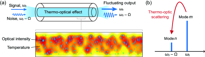
Figure 1: Schematic of TMI in a multimode fiber amplifier. At the fiber input, a signal wave is launched in multiple modes at the same frequency, $\omega_{0}$, with a small amount of noise at the shifted Stokes frequency, $\omega_{0}-\Omega$. As the signal propagates in the fiber, it undergoes amplification due to the stimulated emission, generating heat in the process and causing temperature fluctuations (shown in red in the inset). These temperature variations result in refractive index variations due to the thermo-optical effect, which cause scattering of power between various modes. (Note:longitudinal and transverse dimensions in lower panel are not to scale). (b) The signal in each mode $m$ at $\omega_{0}$ transfers power to the stokes shifted frequency in every other mode $n$, which causes the noise to grow exponentially with a growth rate depending on the signal power and pairwise thermo-optical coupling coefficients. When the noise at the output becomes a significant fraction of the signal, the output beam becomes unstable with dynamic fluctuations on a millisecond timescale. The output power at the onset of significant fluctuations (typically set at $1\%$) is defined as TMI threshold.

We begin by deriving a semi-analytic solution for the optical and heat equations, coupled via the nonlinear polarization and quantum defect heating terms. We expand the optical fields and the temperature fluctuations in terms of eigenmodes of the optical and heat equations respectively. From the driven heat equation, the coefficient of each temperature eigenmode is found in terms of optical amplitudes, leading to coupled amplitude equations for the optical modes, resembling those for a four-wave-mixing processCronin-Golomb et al. (1984). Next, we solve these coupled amplitude equations for an arbitrary input signal at frequency, $\omega_{0}$, along with the presence of small amount of noise at stokes shifted frequencies, $\omega_{0}-\Omega$, in each mode. We show that the noise power in various modes grows exponentially, and can lead to dynamic spatial fluctuations in the output beam profile after sufficiently high noise growth. The growth rate of the noise power in a given mode is equal to the sum of the signal power in each of the other modes, weighted by pairwise thermo-optical coupling coefficients. For any pair of optical modes, the thermo-optical coupling coefficient is proportional to the overlap integrals of the two optical mode profiles with various eigenmodes of the heat equation. The coupling between the optical modes with a large separation in transverse spatial frequency is mediated by temperature modes with high transverse spatial frequency; these thermal modes necessarily have a very short-lifetime, leading to a quite weak coupling between such mode pairs. To study this explicitly, we calculate the thermo-optical coupling coefficients for all $\sim 10^{4}$ mode pairs in a commercially available highly multimode (MM) circular step-index fiber (supporting 82 modes per polarization) and find that the matrix of peak values of pairwise thermo-optical coupling coefficients is a banded, effectively sparse matrix. As a result, the noise growth rate goes down linearly with the number of modes excited, if the power is equally (or nearly equally) distributed in all the excited modes. Therefore the TMI threshold is predicted to increase linearly with the number of equally excited modes, which is verified by explicit calculation of the TMI threshold. Using our theory, we also calculate the thermo-optical coupling coefficients and TMI threshold scaling for multimode fibers with D-shaped and square cross-sectional geometries. The bandedness of the thermo-optical coupling matrix and linear scaling of the TMI threshold is shown to be a generic feature in different fibers, with only the slope of the scaling depending on the specific fiber geometry. The geometry dependence of the slope can be exploited for further TMI threshold enhancement. Our results quantitatively confirm that highly multimode excitations efficiently suppress TMI, opening up a new platform for robust power scaling in high-power fiber laser amplifiers.

II Theory and Results

II.1 Coupled Amplitude Equations

TMI is a result of dynamic transfer of power between fiber modes due to the thermo-optical scatteringJauregui, Stihler, and Limpert (2020); Hansen et al. (2013); Dong (2013). A schematic of the TMI process is shown in Fig. 1. A signal wave at frequency $\omega_{0}$ is sent through an active fiber to undergo optical amplification and generate the output. But due to imperfect coupling or other experimental artifacts, there usually exists a small amount of noise at shifted frequencies, $\omega_{0}-\Omega$, in various modes. The optical signal and noise can interfere to create a spatio-temporally varying optical intensity pattern, which due to the quantum-defect heating that accompanies stimulated emission, results in dynamic temperature variationsJauregui et al. (2012). These spatio-temporal thermal fluctuations result in refractive index variations, which can cause significant transfer of power from signal at $\omega_{0}$ in one mode to the noise at Stokes-shifted frequencies $\omega_{0}-\Omega$ in other modes. As a result, at high-enough output power, the noise in various modes can become a significant fraction of the output power, leading to fluctuations in the output beam profile. This output power level is defined as the TMI thresholdDong (2013); Hansen et al. (2013) and marks the onset of unstable regime for the output. To derive a formalism to calculate the TMI threshold, we solve the optical wave equation with a temperature dependent nonlinear polarization as a source termDong (2013):

$$\nabla^{2}\vec{E}-\frac{n_{0}^{2}}{c^{2}}\frac{\partial^{2}\vec{E}}{\partial t^{2}}=\mu_{0}\frac{\partial^{2}\vec{P}_{\rm NL}}{\partial t^{2}},$$ (1)

where $\vec{E}$ is the total electric field , $c$ is the speed of light and $n_{0}$ is the linear refractive index of the fiber. The temperature-dependent polarisation is given by:

$$\vec{P}_{\rm NL}=\epsilon_{0}\eta\Delta T\vec{E}.$$ (2)

Here, $\eta$ is the thermo-optic coefficient of the fiber material and $\Delta T$ represent the local temperature fluctuation due to quantum-defect heating. $\Delta T$ satisfies the heat equation with a source term proportional to the local intensityHansen et al. (2013):

$$[\nabla^{2}-\frac{\rho C}{\kappa}\frac{\partial}{\partial t}]\Delta T=\frac{Q}{\kappa},$$ (3)

$$Q(r,t)=gq_{\rm D}I(r,t).$$ (4)

The heat source $Q$ is proportional to the local optical intensity $I$, the linear gain coefficient $g$, and the quantum defect $q_{\rm D}=(\frac{\lambda_{\rm s}}{\lambda_{\rm p}}-1)$, which depends on the difference between the signal wavelength $\lambda_{\rm s}$ and pump wavelength $\lambda_{\rm p}$. The thermal conductivity, the specific heat, and the density of the material are given by $\kappa$, $C$ and $\rho$, respectively. The ratio, ${\rho C}/{\kappa}$ is equal to the diffusion constant $D$. Since the thermo-optical polarization depends on the temperature, which in turn depends on the optical intensity, the optical and heat equations are coupled and nonlinear due to the source terms on the right hand side (RHS) of Eq. 1 and Eq. 3. For a translationally invariant system, such as an optical fiber, both optical and heat equations can be solved formally by expanding the fields in terms of the eigenmodes of the linear operator corresponding to each equation. As usual, we decompose the electric field $\vec{E}$ as a sum of the product of transverse mode profile, a rapidly varying longitudinal phase term, and slowly varying amplitude (SVA) for each fiber mode:

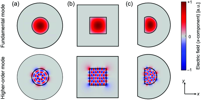
Figure 2: Amplitude profile of guided optical fundamental modes (FM) and higher order modes (HOM) for fibers with three different core shape (a) circular (b) square and (c) D-shaped. The cladding (dotted line) has the same shape as core in each case. Cladding and core sizes are not to scale. The FMs in all three cases fill the core and do not have any nodes. For the circular fiber every HOM has $u$ azimuthal nodes and $v-1$ radial nodes and is referred to as $\rm LPuv$ in standard notation. Here we have shown $\rm LP44$. For square fiber we have considered $x$-polarized TE modes, the mode $\rm TEuv$ has $u$ nodes along the $x$-axis and $v$ nodes along the $y$-axis. Here we have shown $\rm TE85$ mode. The HOMs in D-shaped fiber have a random structure as D-shaped cavities are wave-chaotic.

$$E(r,t)=\int_{-\infty}^{\infty}d\Omega\sum_{m}A_{m}(\Omega,z)\vec{\psi}_{m}(r_{\bot})e^{i((\omega_{0}-\Omega)t-\beta_{m}z)}+{\rm c.c.}$$ (5)

Here, $A_{m}(\Omega,z)$ is the SVA in mode $m$ at a point $z$ along the fiber axis and for a Stokes frequency shift, $\Omega$ from the central frequency $\omega_{0}$. The $\Omega=0$ amplitude corresponds to the signal, and $\Omega\neq 0$ corresponds to the noise. $\vec{\psi}_{m}$ and $\beta_{m}$ denote the transverse mode profile and propagation constant for mode $m$ and can be obtained by solving the fiber modal equationOkamoto (2021); Snyder and Young (1978):

$$\nabla_{T}^{2}\vec{\psi}_{m}+(\frac{n_{0}^{2}\omega_{0}^{2}}{c^{2}}-\beta_{m}^{2})\vec{\psi}_{m}=0.$$ (6)

The solutions to Eq. 6 correspond to the guided fiber modes, which are confined to the fiber core by total internal reflection. These modes can be calculated using a numerical solver such as COMSOLcom for an arbitrary fiber cross-section geometry. As an example, in Fig. 2 we have shown electric field profiles for the FMs and HOMs for step-index fibers with three different cross-sectional geometries: circular, square and D-shaped. The width of the core in each case in 40 $mu\rm m$ and the cladding width is 200 $mu\rm m$. The D-shaped cross-section is obtained by cutting a circle with straight line at a distance equal to half the radius from the centre. In all three cases, the FMs have no node in the electric field profile and follow the symmetries of the cross-section geometry. Each HOM for the circular fiber can be labelled as linearly polarized (LP) mode and characterized by two indices $(u,v)$ in the standard notationOkamoto (2021). The mode ${\rm LP}uv$ has $u$ azimuthal nodes and $(v-1)$ radial nodes, with a radial profile given by the $(u+1)^{\rm th}$ Bessel function of the first kind, with $v-1$ zeros within the fiber core and angular profile given by either a sine or cosine function with $u$ zeros. Figure 2a shows the profiles of $\rm LP01$ (FM) and $\rm LP44$ (HOM) modes. For the square cross-section, the HOMs can be labelled as transverse electric (TE) modesMarcatili (1969) and characterized by two indices $(u,v)$. The electric field in the $\rm TEuv$ mode is given by the product of sine(s) and/or cosine(s) in both $x$ and $y$ directions with $u$ nodes in $x$ and $v$ nodes in $y$ within the fiber core. The D-shaped fiber results in modes with random structures. This is due to the fact that D-shaped cavities are wave-chaoticBittner et al. (2020), leading to ergodic field distributions.

Normalizing each mode profile $\psi_{m}$ to have unit power, the total power in mode $m$ at point $z$ along the fiber axis and at Stokes frequency $\Omega$ is given by ${|A_{m}(z,\Omega)|}^{2}$. The heat source term $Q$ in Eq. 3 can be obtained in terms of optical modal amplitudes using Eq. 4 and Eq. 5. The optical intensity $I$ contains terms corresponding to the interference of various fiber modes, and thus $Q$ ($\propto I$) is given by a sum of dynamic heat sources oscillating at Stokes frequency $\Omega$ and propagation constant $q_{ij}=\beta_{j}-\beta_{i}$ for each mode pair $\{i,j\}$. Thus, we expand $\Delta T$ into a series of temperature profiles corresponding to each heat source term:

$$\Delta T(r,t)=\int_{-\infty}^{\infty}d\Omega\sum_{i,j}T_{ij}(r,\Omega)e^{i(\Omega t-q_{ij}z)}.$$ (7)

Here $T_{ij}(r,\Omega)$ is the profile of the temperature grating with longitudinal wavevector $q_{ij}$ and temporal frequency $\Omega$. We further decompose each temperature profile $T_{ij}$ in terms of the eigenmodes of the transverse Laplacian $\nabla_{T}^{2}$:

$$T_{ij}(r,\Omega)=\sum_{k}a^{k}_{ij}(z,\Omega)\tilde{T}^{k}(r_{\perp}).$$ (8)

Here, $a^{k}_{ij}$ is the SVA for temperature eigenmode $k$ in temperature grating $\{i,j\}$. $\tilde{T}^{k}$ denotes the transverse profile of temperature eigenmode $k$ which satisfies the following eigenvalue equation:

$$\nabla_{T}^{2}\>\tilde{T}^{k}(r_{\perp})=-\alpha_{k}^{2}\>\tilde{T}^{k}(r_{\perp})\>\>,\>\>\>\>\tilde{T}^{k}|_{\partial\Omega}=0.$$ (9)

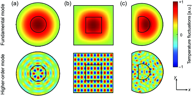
Figure 3: Profile of temperature fluctuations in various eigenmodes of the heat equation with constant temperature on the cladding surface for fibers with three different cladding shapes (a) circular (b) square and (c) D-shaped. The core (dotted line) has the same shape as cladding in each case. Cladding and core sizes are not to scale. The temperature fluctuations in each mode are spread out over both core and cladding. The lowest order modes (fundamental modes) in all three cases fill the entire fiber cross-section and do not have any nodes. For the circular fiber every HOM has $u$ azimuthal nodes and $v-1$ radial nodes over the whole cross-section. Here we have shown mode with $u=4$ and $v=7$. For the square fiber every HOM has $u$ nodes along $x$-axis and $v$ nodes along $y$-axis over the whole cross-section. Here we have shown mode with $u=11$ and $v=8$. The HOMs in D-shaped fiber have a random structure with increasing number of nodes with mode order.

$\nabla_{T}^{2}$ is a self-adjoint operator, thus its eigenmodes $\{\tilde{T}^{k}\}$ form a complete and orthogonal basis, with $-\alpha_{k}^{2}$ as the eigenvalue for eigenmode $k$. We impose Dirichlet boundary conditions at the outer surface of the fiber, corresponding to the standard assumptionDong (2013) that outer surface is held at a constant temperature, and all the heat immediately dissipates into a heat bath. The temperature eigenmodes can be solved either analytically or numerically depending on the fiber geometry. We have shown in Fig. 3 the fundamental and higher-order temperature eigenmodes for three different cladding geometries: circular, square, and D-shaped, which are calculated using the Coefficient-Form-PDE module in COMSOLcom . The spatial structure of the temperature eigenmodes are similar to the optical modes since both are eigen-functions of same spatial operator $\nabla_{T}^{2}$. An important distinction is that optical modes are localised in the fiber core, but the temperature eigenmodes spread out over the entire fiber cross-section, due to the differing boundary conditions. The fundamental modes have no nodes and follow the symmetries of the cladding geometry. For the circular cladding, the eigenmodes are characterised by $u$ azimuthal and $v$ radial nodes across the entire fiber cross-section (i.e., core plus cladding), with a radial dependence given by $(u+1)^{\rm th}$ Bessel function of the first kind and angular dependence given by sine or cosine with $u$ zeros. For the square cladding, the eigenmodes are given by the product of sine(s) and/or cosine(s) in both $x$ and $y$ dimensions with an integer number of nodes across the entire core and cladding. Similar to the optical modes, the D-shaped fiber exhibits temperature modes with irregular structures, except for the reflection symmetry about the $x$ axis, due to the chaotic nature of D-shaped cavities.

To complete the solution for $\Delta T$, we need to determine each coefficient $a^{k}_{ij}$. This is done by simplifying the LHS of Eq. 3 by substituting $\Delta T$ from Eq. 7 and Eq. 8 and using the eigenmode equation Eq. 9. The RHS of Eq. 3 can be obtained in terms of optical amplitudes by using Eq. 4 and Eq. 5. Finally, by exploiting orthogonality, we isolate the desired coefficient $a^{k}_{ij}$ by multiplying both sides of simplified Eq. 3 with $\tilde{T}^{k*}$ and integrating it across the fiber cross-section leading to:

$$a^{ij}_{k}(z,\Omega)=\frac{D\langle\vec{\psi}_{i}^{*}\cdot\vec{\psi}_{j}\tilde{T}_{k}^{*}\rangle}{\Gamma_{k}^{ij}+i\Omega}\frac{gq_{\rm D}}{\kappa}\int_{-\infty}^{\infty} d\Omega^{\prime}A_{i}^{*}(z,\Omega^{\prime})$$ (10)

$$A_{j}(z,\Omega+\Omega^{\prime}).$$

The amplitude of temperature eigenmode $k$ for the heat source term $\{i,j\}$ is proportional to the overlap of the dot product of $\vec{\psi}_{i}$ and $\vec{\psi}_{j}$ with the temperature mode profile $\tilde{T}^{k}$ integrated over the fiber cross-section, denoted by the angular brackets $\langle.\rangle$. It is also proportional to the convolution of optical amplitudes $A_{i}$ and $A_{j}$. We introduce an inverse mode lifetime for mode $k$ given by $\Gamma_{k}^{ij}={((\beta_{i}-\beta_{j})}^{2}+\alpha_{k}^{2})D$ with units of $[s^{-1}]$. The first term in the inverse mode lifetime corresponds to the longitudinal heat diffusion, and the second term corresponds to the transverse heat diffusion. In typical fibers, the transverse heat diffusion dominates, so the longitudinal heat diffusion can be ignoredHansen et al. (2013); Dong (2013). In that case, we can define $\Gamma_{k}^{ij}\approx\Gamma_{k}=\alpha_{k}^{2}D$, which we use in the rest of this paper. However, in fibers where longitudinal diffusion is significant, both contributions need to be included in the inverse mode lifetime. This completes the formal solution for $\Delta T$ in terms of the optical mode profiles and amplitudes.

Next, we use the solution for $\Delta T$ to evaluate the source terms in Eq. 1, which can be used to derive coupled self consistent equations for optical amplitudes. We use the ansatz for $\vec{E}$ from Eq. 5 to simplify the left hand side (LHS) of Eq. 1. Finally we use the orthogonality of the optical modes to isolate the equation of each optical amplitude $\{A_{m}\}$ by multiplying both sides of simplified Eq. 1 with $\vec{\psi}_{m}^{*}$ and integrating it over the fiber cross-section:

$$\diff{A_{m}(z,\Omega)}{z}= \frac{g}{2}A_{m}+ig\chi_{0}\sum_{ijn}\int d\Omega^{\prime}A_{n}(z,\Omega-\Omega^{\prime})$$ (11)

$$G_{mnij}(\Omega^{\prime})\int d\Omega^{{}^{\prime\prime}}A_{i}^{*}(z,\Omega^{{}^{\prime\prime}})A_{j}(z,\Omega^{\prime}+\Omega^{{}^{\prime\prime}})$$

$$e^{i(\beta_{m}-\beta_{n}+\beta_{i}-\beta_{j})z}.$$

The $z$ derivative of the modal amplitude $A_{m}$ has contributions from both the linear amplification term with growth rate $g/2$ due to stimulated emission and a nonlinear four-wave-mixing termCronin-Golomb et al. (1984) due to the thermo-optical interaction, which is proportional to a susceptibility constant $\chi_{0}$ and the sum of convolutions of three modal amplitudes $A_{n}$, $A_{i}^{*}$, and $A_{j}$. The exponential term tracks the phase mismatch for each contribution, and the strength of each term is proportional to the overlap of the Green’s function of the heat equation with the relevant optical mode profiles:

$$G_{mnij}(\Omega)=\sum_{k}\frac{D\langle\vec{\psi}_{i}^{*}\cdot\vec{\psi}_{j}\tilde{T}_{k}^{*}\rangle\langle\tilde{T}_{k}\psi_{m}^{*}\psi_{n}\rangle}{\Gamma_{k}+i\Omega},\>\>\>\>\chi_{0}=\frac{\eta q_{\rm D}k_{0}}{2n_{c}\kappa}.$$ (12)

The sum over $k$ represents the sum over all the temperature eigenmodes. Thus, $G_{mnij}(\Omega)$ denotes the optical modal overlap with the Green’s function of the heat equation written in the spectral representationCole et al. (2010). The susceptibility constant $\chi_{0}$ involves a combination of various material and optical constants involved and has dimensions of $[W^{-1}]$. $G_{mnij}(\Omega)$ has both real and imaginary parts in general. The real part is responsible for the nonlinear phase evolution of $A_{m}$, while the imaginary part is responsible for dynamic transfer of power between various modes. Clearly, for $\Omega=0$, the imaginary part of $G_{mnij}$ vanishes and thus there is no transfer of power between various modes of the fiber at $\omega_{0}$. A nonzero Stokes frequency shift is needed for TMI, which is in agreement with the well known result that a moving intensity grating ($\Omega\neq 0$) is required for TMIJauregui et al. (2012); Hansen et al. (2013); Robin, Dajani, and Pulford (2014); Jauregui, Stihler, and Limpert (2020). Typically there is amplitude noise in the fiber, either due to experimental imperfections or due to spontaneous emission, having multiple frequency components. The noise frequency at which imaginary part of Green’s function peaks undergoes the highest amplification and is typically a few $~{}kHz$, leading to dynamic fluctuations in the beam profile on the order of millisecondsHansen et al. (2013); Jauregui et al. (2011); Jauregui, Stihler, and Limpert (2020).

For any given set of input amplitudes in each mode, $\{A_{m}(z=0,\Omega)\}$, Eq. 11 can be solved to obtain modal amplitudes $\{A_{m}(z,\Omega)\}$ everywhere, fully determining both $\vec{E}$ and $\Delta T$. The fiber properties are taken into account through $\chi_{0}$ and $G_{mnij}$ via optical mode profiles $\{\psi_{m}\}$ and temperature mode profiles $\{\tilde{T}^{k}\}$. Equation 11 is a set of highly coupled nonlinear differential equations, and in general cannot be solved analytically. Numerical solutions are possible by using finite difference methodsSun, Zhang, and Gao (2023) to discretize the derivative operator and evaluating the convolutions by either built-in or custom operations. It is expected that numerically solving Eq. 11 would be more computationally efficient than solving the original coupled optical and heat equations. This is because Eq. 11 is a set of 1D equations, where transverse degrees of freedom are accounted through the fiber modes, which exploit the longitudinal translation invariance and only need to be solved once for a given fiber. However, despite this simplification, when a large number of modes are present, the computational complexity can quickly become very high. Additionally, for studying TMI suppression using multimode excitation, the input modal content needs to be parametrically tuned, requiring a fast and efficient solution. Fortunately, an approximate solution to the coupled amplitude equations can be obtained that captures the essential features of the onset of TMI and can be used to calculate the TMI threshold, which is derived in the next section.

II.2 Phase-Matched Noise Growth

In this section, we derive an approximate solution to the coupled amplitude equations to study noise growth due to thermo-optical scattering when signal power is launched into multiple fiber modes. We utilize two key approximations: (1) we retain only the phase-matched termsHansen et al. (2013); Dong (2013, 2022); Menyuk et al. (2021), since phase-mismatched terms become insignificant over long enough length scales, and (2) we assume that the noise power is significantly lower than the signal power, and the change in the signal due to the noise growth is ignoredZervas (2017); Hansen et al. (2013); Dong (2013). This is typically valid below the TMI threshold, which marks the onset of significant beam fluctuations, and can be used to calculate the threshold. We assume that at the fiber input, the signal (or, seed) is injected at frequency $\omega_{0}$ in various modes with complex amplitudes $\{A^{\rm s}_{m}(z=0)\}$. In addition, there is noise present at Stokes shifted frequencies $\omega_{0}-\Omega$ in all the fiber modes, denoted by complex amplitudes $\{B_{m}(z=0,\Omega)\}$. The total input amplitude in mode $m$ can be written as:

$$A_{m}(z=0,\Omega)=A^{\rm s}_{m}(z=0)\delta(\Omega)+B_{m}(z=0,\Omega).$$ (13)

Similarly, the total amplitude in mode $m$ at any point $z$ can be decomposed into the signal ($\Omega=0$) and noise ($\Omega\neq 0$) amplitudes:

$$A_{m}(z,\Omega)=A^{\rm s}_{m}(z)\delta(\Omega)+B_{m}(z,\Omega).$$ (14)

As the light propagates down the fiber, both the signal and noise grow exponentially due to the linear optical gain $g$. Below the TMI threshold, signal amplitudes roughly grow independently of the noise and in the case of no gain saturation are given by:

$$A^{\rm s}_{m}(z)=A^{\rm s}_{m}(0)e^{\frac{g}{2}z}e^{i\phi^{\rm NL}_{m}}.$$ (15)

Here, $\phi^{\rm NL}_{m}$ is the nonlinear phase evolution in mode $m$. More importantly, noise also grows due to the transfer of power from the signal due to the thermo-optical scattering. The noise growth can be obtained by solving Eq. 11, which is first simplified by retaining only the phase-matched terms, given by the condition $\beta_{m}-\beta_{n}+\beta_{i}-\beta_{j}=0$, leading to:

$$\diff{A_{m}(z,\Omega)}{z}= \frac{g}{2}A_{m}+ig\chi_{0}\sum_{n}\int d\Omega^{\prime}A_{n}(z,\Omega-\Omega^{\prime})$$ (16)

$$G_{mnnm}(\Omega^{\prime})\int d\Omega^{{}^{\prime\prime}}A_{m}^{*}(z,\Omega^{{}^{\prime\prime}})A_{n}(z,\Omega^{\prime}+\Omega^{{}^{\prime\prime}}).$$

We have utilized $m=j,i=n$ as a straightforward solution to the phase-matching condition, reducing the triple sum in the second term of Eq. 11 to a single sum in Eq. 16. Note that although $m=n,i=j$ is also a valid solution to the phase-matching condition, such terms correspond to only a cross-phase modulation but no transfer of power as these terms result in only a uniform temperature shift ($q_{ij}=0$), thus we do not retain these terms. Next, we substitute the ansatz for $A_{m}$ from Eq. 14 and Eq. 15 in Eq. 16 and simplify the RHS to obtain the equation growth equation for $B_{m}(z,\Omega)$:

$$\frac{dB_{m}(z,\Omega)}{dz}=g(\frac{1}{2}+i\chi_{0}\sum_{n}G_{mnnm}(\Omega)P^{\rm s}_{n}(z))B_{m}(z,\Omega).$$ (17)

All the terms which are quadratic or higher order in noise amplitudes are ignored. Each noise amplitude grows exponentially, independently of other noise amplitudes, and has contributions in growth rate from both linear amplification and nonlinear power transfer from the signal. $P^{\rm s}_{m}$ represents the signal power in mode $m$ and is given by ${|A^{\rm s}_{m}|}^{2}$ and $G_{mnnm}$ represents the contribution to noise growth in mode $m$ by signal power in mode $n$. We can convert noise amplitude growth equations for mode $m$ into growth equations for noise power (given by $|B_{m}|^{2}$), by multiplying with $B_{m}^{*}$ on both sides and adding the complex conjugate term:

$$\frac{dP^{\rm N}_{m}(z,\Omega)}{dz}=g(1+\sum_{n\neq m}\chi_{mn}(\Omega)P^{\rm s}_{n}(z))P^{\rm N}_{m}(z,\Omega).$$ (18)

Here, $P^{\rm N}_{m}$ denotes the noise power in mode $m$. The first term on the RHS in Eq. 17 corresponds to linear optical gain and each term in the second term corresponds to a transfer of power from a particular signal mode $n$ to noise in mode $m$ due to the thermo-optical scattering. We have ignored the self-coupling termHansen et al. (2013) (corresponding to $G_{mmmm}$) since it is not responsible for intermodal power transfer. For each mode pair $(m,n)$, we have defined a thermo-optical coupling coefficient $\chi_{mn}(\Omega)$, which is equal to $-2$ times the imaginary part of $G_{mnnm}$ multiplied with $\chi_{0}$. Eq. 18 can be solved analytically, resulting in exponential growth in noise power in each mode $m$:

$$P^{\rm N}_{m}(L,\Omega)=P^{\rm N}_{m}(0,\Omega)e^{gL}e^{G^{\tiny{\rm TMI}}_{m}(\Omega)}.$$ (19)

$P^{\rm N}_{m}(0,\Omega)$ represents noise power in mode $m$ at the input end of the fiber. $P^{\rm N}_{m}(L,\Omega)$ is the noise power at the output upon exponential growth both due to the linear gain $g$ and the TMI gain which depends on signal power distribution:

$$G^{\tiny{\rm TMI}}_{m}(\Omega)=\sum_{n\neq m}\chi_{mn}(\Omega)\int_{0}^{L}gP_{n}^{\rm s}(z)dz$$ (20)

The $z$ integral can be simplified by using the signal growth formula given in Eq. 15, $\int_{0}^{L}gP_{n}^{\rm s}(z)dz=P_{n}^{\rm s}(L)-P_{n}^{\rm s}(0)\approx\Delta P\tilde{P}^{\rm s}_{n}$, where $\Delta P$ is the total signal power extracted from the amplifier and $\tilde{P}^{\rm s}_{n}$ is the fraction of signal power in mode $n$ ($\sum_{n}\tilde{P}_{n}^{\rm s}=1$), which is determined by the input excitation. Thus, TMI gain in mode $m$ is given by:

$$G^{\tiny{\rm TMI}}_{m}(\Omega)=\Delta P\sum_{n\neq m}\chi_{mn}(\Omega)\tilde{P}_{n}^{\rm s}.$$ (21)

This formula suggests a relatively straightforward interpretation. The TMI gain for any mode depends on the total extracted signal power and effective thermo-optical coupling coefficient, which is given by the weighted sum of thermo-optical coupling coefficients with all the other modes, with weights depending on the input excitation. For a two-mode fiber with FM-only excitation ($\tilde{P}^{\rm s}_{1}=1$), the above formula reduces to the well known formula for TMI gainDong (2013); Hansen et al. (2013), where it is given by the product of extracted signal power and the thermo-optic coupling between the two modes $\chi_{21}$. More generally, Eq. 21 can be used to derive the formula for the TMI threshold under arbitrary multimode excitations, as shown in the next section.

II.3 Multimode TMI Threshold

The TMI threshold is defined as the total output power when the noise power becomes a significant fraction ($\xi>1\%$) of the signal power, which leads to the onset of a fluctuating beam profileHansen et al. (2013); Dong (2013). For a given amount of input noise power, this occurs when the highest TMI gain across all frequencies and modes becomes large enough. Therefore, a quantitative condition for the threshold can be derived from Eq. 19 and Eq. 21:

$$P^{\rm N}(L)=P^{\rm N}(0)\>\>e^{gL}e^{(P_{\rm th}-P^{\rm s}(0))\bar{\chi}}=\xi P^{\rm s}(0)e^{gL},$$ (22)

which can be rearranged as:

$$(P_{\rm th}-P^{\rm s}(0))\bar{\chi}=\log(\frac{\xi P^{\rm s}(0)}{P^{\rm N}(0)}),$$ (23)

where, $P_{\rm th}$ is the TMI threshold, $L$ is the length of the fiber, $P^{\rm s}(0)$ and ${P^{\rm N}(0)}$ are the input signal and noise powers, respectively. We have introduced an overall thermo-optical coupling coefficient $\bar{\chi}$ which is equal to the maximum value of the effective thermo-optical coupling coefficients across all the modes and Stokes frequencies:

$$\bar{\chi}=\max_{\Omega,m}\sum_{n\neq m}\chi_{mn}(\Omega)\tilde{P}_{n}^{\rm s}.$$ (24)

A key insight from the multimode TMI threshold formula in Eq. 23 is that TMI threshold is roughly inversely proportional to the overall thermo-optical coupling coefficient $\bar{\chi}$, which depends on both the fiber properties through $\chi_{mn}$ and the input power distribution, ${\tilde{P^{\rm s}_{n}}}$. It also depends weakly (logarithmically) on the input noise power and the noise fraction $\xi$ at which the threshold is set. Also, any increase in input signal power (or, seed power) leads to a corresponding increase in the TMI threshold. Typically the input power is significantly smaller than the TMI threshold, thus the overall relative change due to a seed power increase is smallTao, Wang, and Zhou (2018); Dong (2022). It can be easily verified that when only the fundamental mode is excited ($\tilde{P}_{1}=1,\tilde{P}_{n\neq 1}=0$), the overall thermo-optical coupling coefficient, $\bar{\chi}$ simplifies to $\chi_{21}$, reducing our multimode TMI threshold formula to a previously derived formula in studies which only consider single mode excitationDong (2013). More generally, multimode excitation provides a parameter space to control the overall thermo-optical coupling coefficient and the TMI threshold, even for a fixed fiber. The TMI threshold is highest for the signal power distribution which minimizes the maximum effective thermo-optical coupling coefficient. The amount of tunability therefore depends on the properties of the pairwise thermo-optical coupling coefficients which we discuss in detail in the next section.

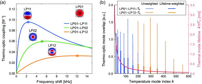
Figure 4: (a)Thermo-optical coupling coefficient between the FM (LP01) and three HOMs in increasing mode order (LP11, LP02, LP12) for circular fiber . Relevant mode profiles are shown in the insets. The thermo-optical coupling coefficient vanishes for zero Stokes shift ($\Omega=0$) and peaks at frequencies on the order of few KHz. LP01 couples most strongly with LP11 (blue curve) and the peak coupling decreases with increasing transverse spatial frequency mismatch between the modes (green and orange curves). The peak frequency and linewidth also increases with mode order of HOMs. (b) thermo-optical mode overlap for two different optical mode pairs: LP01-LP11 (blue) and LP01–LP12 (orange) with various temperature eigenmodes. The temperature modes are ordered by increasing eigenvalues and decreasing mode lifetimes, $2\pi\Gamma_{k}^{-1}$ (shown by dotted red curve). For each optical mode pair only a few temperature eigenmodes have significant overlap (dotted bars), the ones which have spatial frequency similar to the frequency of interference pattern of optical modes within the fiber core. For neighboring optical mode pair (LP01–LP11), significant overlap occur with lower order temperature eigenmodes (with high mode lifetime) and for mode pair with relatively larger separation (LP01–LP12), significant overlap occurs with relatively higher order temperature eigenmodes (with short mode lifetimes). Note that the thermo-optical coupling coefficients are decreased when the mode lifetimes $2\pi\Gamma_{k}^{-1}$ are smaller. Consequently, optical mode pairs with larger separation have weaker overall coupling as indicated when the thermo-optical overlaps are weighted by lifetime (solid bars), leading to the lower peak coupling and higher peak frequency as shown in (a).

II.4 Thermo-optical coupling

The thermo-optical coupling coefficient between any modes $m$ and $n$ is proportional to the imaginary part of a particular component of the Green’s function, $G_{mnnm}$, and is equal to:

$$\chi_{mn}(\Omega)=\chi_{0}\sum_{k}|\langle\vec{\psi}_{m}^{*}\cdot\vec{\psi}_{n}\tilde{T}_{k}\rangle|^{2}\frac{D\Omega}{\Gamma_{k}^{2}+\Omega^{2}}.$$ (25)

$\chi_{mn}$ has contributions from each temperature eigenmode $k$. The strength of each contribution is proportional to the integrated overlap of the dot product of the optical mode profiles $\vec{\psi}_{m}$ and $\vec{\psi}_{n}$ with the temperature mode profile $\tilde{T}^{k}$. Each contribution has a characteristic frequency curve which peaks at a frequency given by inverse mode lifetime $\Gamma_{k}$, and the peak value is proportional to the thermal mode lifetime $2\pi\Gamma_{k}^{-1}$. To illustrate the key properties of the thermo-optical coupling coefficient we calculate $\chi_{mn}(\Omega)$ for all the mode pairs of a circular step-index fiber with core diameter of 40 $\mu$m, cladding diameter of 200 $\mu$m and numerical aperture $NA=0.15$, supporting 82 modes per polarization. Detailed fiber or optical parameters used for calculation are provided in Table 1. We consider optical modes linearly polarized (LP) along the $x$-direction. Each LP mode is designated by two indices $[u,v]$ which correspond to the number of azimuthal and radial nodes respectivelyOkamoto (2021); Qian and Huang (1986) (See Fig. 2a). The modes are arranged in the order of decreasing longitudinal propagation constants. For instance, first five modes (excluding rotations) are LP01 (FM), LP11, LP21, LP02, and LP12. In our notation, therefore, $\chi_{12}\equiv\chi_{LP01,LP11}$. Note that LP modes are only approximate modes of the fiber, which become inaccurate for fibers with long lengths, in which case the exact vector fiber modes (HE and EH modes) need to be consideredOkamoto (2021). For the purpose of our discussion we assume that LP modes are accurate enough for the length of the fiber considered.

In Fig. 4a we have shown the thermo-optical coupling coefficient between the FM (LP01) and three HOMs in increasing mode order (LP11, LP02, LP12) for this fiber. Relevant mode profiles are shown in the inset. The thermo-optical coupling coefficient in all three cases is zero at $\Omega=0$ and attains its peak value at frequencies on the order of few kHz, consistent with the millisecond timescale of TMIHansen et al. (2013); Dong (2013); Jauregui, Stihler, and Limpert (2020). The FM couples most strongly with the lowest HOM (blue curve), and the peak coupling decreases with increasing transverse spatial frequency mismatch between the modes (green and orange curves). The peak frequency and linewidth are higher for larger spatial frequency mismatch between the modes. These results can be understood by investigating the specific temperature eigenmodes facilitating the coupling for different mode pairs, as shown in Fig. 4b. The contribution of each temperature eigenmode to the coupling between a pair of optical modes is proportional to (1) the thermo-optical modal overlap integral and (2) the corresponding thermal mode lifetime $2\pi\Gamma_{k}^{-1}$ (Eq. 25). Overall, only a few temperature eigenmodes, which match the transverse intensity profile of the interference between the optical modes, have a significant overlap integral. For $\rm LP01-LP11$ coupling, the optical interference pattern has relatively lower spatial frequencies and thus has significant overlap with relatively lower order temperature eigenmodes (shown by blue dotted bars in Fig. 4b). On the other hand, the LP01–LP12 mode pair has a significant overlap with relatively higher order temperature eigenmodes (shown by orange bars in Fig. 4b). The thermal mode lifetime is shorter for temperature eigenmodes with higher transverse spatial frequency (as shown by red dotted curve in Fig. 4b), so the contribution of higher-order temperature eigenmodes is damped. Such intrinsic dampening of high spatial frequency contributions to the temperature are characteristic of the heat propagation being a diffusive processSeyf and Henry (2016). Consequently the lifetime weighted thermo-optical mode overlap for neighboring optical modes (blue solid bars) is much higher than for modes with larger separation of transverse spatial frequency (orange solid bars). As a result, peak thermo-optical coupling coefficient decreases with increasing spatial frequency mismatch between the optical modes.

Parameter	Value
Core shape	Circular
Core diameter [$\mu$m]	40
Cladding diameter [$\mu$m]	200
Core refractive index	1.458
Cladding refractive index	1.45
Signal wavelength, $\lambda_{\rm s}$ [nm]	1064
Pump wavelength, $\lambda_{\rm p}$ [nm]	976
Number of optical modes	82
Thermo-optic coefficient, $\eta$ $[{\rm K}^{-1}]$	$3.5\times 10^{-5}$
Thermal conductivity, $\kappa$ $[{\rm Wm}^{-1}{\rm K}^{-1}]$	$1.38$
Diffusion constant $D$ $[{\rm m}^{2}{\rm s}^{-1}]$	$8.46\times 10^{-7}$

Table 1: Detailed parameters for circular fiber.

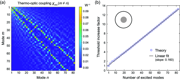
Figure 5: (a) Thermo-optical coupling matrix for circular fiber (Circular cross-section). Each element ${m,n}$ is a positive entry given by the peak value of thermo-optical coupling coefficient $\chi_{mn}(\omega)$. Self-coupling is not considered ($m=n$). Only a few entries close to the diagonal have significant value, giving a banded matrix. (b) TMI threshold scaling in circular fiber with the number of equally excited modes $M$. Threshold increase factor is defined by taking the ratio of TMI threshold with the threshold for FM-only excitation. As the number of excited modes are increased, the TMI threshold increases linearly and can reach upto $13$ times higher when all $82$ modes are excited.

This is a generic result for all optical mode-pairs. To explicitly show this, we calculate the peak value of $\chi_{mn}(\Omega)$ for all $\sim 10^{4}$ mode pairs in circular fiber . The resulting coupling matrix is shown in Fig. 5a as a false color image. We have omitted the self coupling ($m=n$), since it is not responsible for intermodal power transfer between the modesHansen et al. (2013). Clearly, every mode couples strongly with only a few modes resulting in a highly banded/sparse coupling matrix. The strong coupling occurs when the spatial frequencies of two modes are closely matched, i.e., similar number of radial and azimuthal nodes ($\Delta u,\Delta v\leq 1$). As we will see below, this banded nature of the coupling matrix is what allows a significant suppression of TMI upon multimode excitation.

II.5 Threshold Scaling

Recall that the TMI threshold is defined as the output signal power at which the noise power in any mode becomes a significant fraction ($>1\%$) of the output signal powerDong (2013), and the beam profile fluctuates dynamically rendering it useless for many applicationsJauregui, Stihler, and Limpert (2020). According to Eq. 23 and Eq. 24, the TMI threshold is inversely proportional to the overall thermo-optical coupling coefficient $\bar{\chi}$ which is a sum of $\chi_{mn}$ weighted by the fraction of signal power in each mode, which depends on the input excitation. Most previous TMI suppression efforts consider exciting only the fundamental mode and avoid sending power in HOMs, which our results indicate is not the optimal approach. To show this explicitly we consider two special cases of input excitation — (1) FM-only excitation: all of the signal power is present in the FM ($\tilde{P}_{1}^{\rm s}=1$) and noise is present in HOMs, and (2) Equal mode excitation : the input power is divided equally in $M$ modes of the fiber($\tilde{P}_{n}^{\rm s}=1/M$). We use Eq. 24 to calculate $\bar{\chi}$ in the two cases and use it to compare the TMI threshold. In the first case, the noise in the first HOM ($m=2$) has the highest growth rate due to signal power in the FM ($m=1$), giving $\bar{\chi}=\chi_{21}$. Since $\chi_{21}$ is the highest coupling out of all mode pairs (Fig. 5a), FM-only excitation actually leads to the lowest TMI threshold. In the second case, all the modes contribute to the overall coupling to a given mode (say, $m=2$) but with weights reduced by a factor of $M$ i.e., $\bar{\chi}=\sum_{n\neq 2}\chi_{2n}/M$. Due to the banded nature of $\chi_{mn}$ only a few elements in the sum are significant, leading to $\bar{\chi}\approx{s\chi_{21}}/{M}$. Here, $s$ is used to denote the average number of significant elements in the any row of the thermo-optical coupling matrix, which does not scale with $M$ and is roughly equal to 6 for circular fiber. Thus, for a highly multimode excitation ($M\gg s$), the TMI threshold can be significantly higher than the FM-only excitation. In fact, our reasoning predicts that the TMI threshold will increase linearly with the number of equally-excited modes, $M$. To verify this explicitly, we calculate the TMI threshold as $M$ is increased. We define the threshold increase factor (TIF) as the ratio of TMI threshold for $M$-mode excitation with that for FM-only ($M\approx 1$) excitation. Fig. 5b shows the values of TIF as $M$ is varied. As predicted, the TMI threshold increases linearly with number of excited modes with a slope roughly equal to $1/{\rm s}$ $(\approx 0.16)$. When all 82 modes in the circular fiber are excited equally, we find a remarkable 13$\times$ enhancement of the TMI threshold over FM-only excitation. This confirms that highly multimode excitation in a multimode fiber amplifier can be a great approach for achieving robust TMI suppression.

It should be noted that although we have only considered equal-mode excitation to achieve a higher TMI threshold, it is by no means a strict condition. Our theory predicts that multimode excitation will generically lead to a higher threshold than the FM-only excitation. This follows directly from the banded nature of the thermo-optical coupling matrix, which is a consequence of the diffusive nature of the heat equation. Therefore, it is expected to be a universal result, independent of the details of fiber composition and geometry. The level of enhancement will depend on the effective number of excited modes. While most previous studies of TMI consider FM-only excitation, an increase in TMI threshold due to multimode excitation has been observed in some cases. A recent study by the current authors demonstrated an increase in TMI threshold upon multimode excitation using explicit time-domain numerical simulations of coupled optical and heat equations in 1D-cross-section waveguidesChen et al. (2023b). Additionally, several recent experimental studies on the effect of fiber bending on TMI threshold in few-mode fibers provide evidence for our predictionsZhang et al. (2019); Wen et al. (2022); Li et al. (2023). They have observed that upon launching light in a fiber that supported multiple modes, a higher TMI threshold is obtained for a larger bend diameter (i.e., a loosely coiled fiber). The bend-loss of HOMs decreases when the bend diameter is larger, and thus the effective number of excited modes is higher, which leads to a higher TMI threshold in accordance with our predictions. It should be noted that these experimental findings are opposite to the predictions of previous theories which only consider FM excitation and predict that decreased HOM loss upon increasing bend diameter should lead to lowering of the TMI thresholdDong (2023); Tao et al. (2016). The authors of these studiesWen et al. (2022); Zhang et al. (2019) pointed out this anomaly and tried explaining these results by arguing that lower mode mixing leads to a higher threshold. In our opinion, this discrepancy is a result of ignoring the signal power in HOMs which is fully taken into account in our formalism. These results are straightforwardly explained by our theory.

III Impact of Fiber Geometry

So far, we have considered a standard step-index multimode fiber with a circular cross-section, which shows that TMI threshold increases linearly with number of excited modes owing to the banded nature of the thermo-optical coupling matrix. This banded nature is a fundamental consequence of the diffusive nature of the heat propagation which underlies the thermo-optical scattering due to the intrinsic damping of high-spatial-frequency features. As a result, we expect the banded nature of the thermo-optical coupling matrix to be maintained even in fibers with non-standard geometriesVelsink et al. (2021); Ying et al. (2017); while the number of significant elements in the coupling matrix, and their relative values can depend on the particular fiber geometry. As such, we expect the linear scaling of the TMI threshold to be maintained, but the slope to differ for fibers with different cross-sectional geometries. Thus studying different fiber geometries to determine which yields a higher slope of threshold increase with $M$ may be useful in designing fibers with enhanced TMI thresholds.

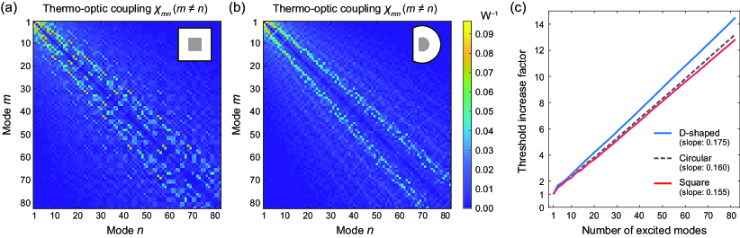
Figure 6: Thermo-optical coupling matrix for (a) square fiber (b) D-shaped fiber. Self-coupling is not considered ($m=n$). Similar to circular fiber, the thermo-optical coupling matrices for both square fiber and $C$ are also banded. (b) As a result TMI threshold in square fiber (red) and D-shaped fiber (blue) also increases linearly with the number of equally excited modes $M$. The slope of the scaling is highest for D-shaped fiber and lowest for square fiber. The scaling for circular fiber is reproduced as the dotted curve for reference.

As our formalism does not assume any particular fiber cross-section geometry, unlike most previous approachesDong (2013); Hansen et al. (2013); Zervas (2017), it can be utilized straightforwardly for calculating the TMI threshold for different fiber geometries under multimode excitation. We consider two additional fiber cross-sectional geometries other than circular: square fiber and D-shaped fiber (referring to a circular shape truncated by removing a section bounded by a chord). A reason to study these particular shapes is because square and D-shaped cross-sections support modes with statistically different profiles. While a square shape results in an integrable transverse "cavity", supporting modes with regular spatial structureMarcatili (1969)(as does the circular fiber); in contrast, the D-shaped cross-section leads to wave-chaotic behavior in the transverse dimensions, with highly irregular and ergodic modesBittner et al. (2020). Due to this property, D-shaped micro-cavities have found applications in suppressing instabilities and speckle-free imaging in 2D semiconductor micro-lasersBittner et al. (2018); Redding et al. (2015). Similar to the circular fiber, the square fiber is chosen to have a core width of 40 $\mu$m and a cladding width of 200 $\mu$m. For the square fiber, we consider a slightly smaller NA (0.135) as it has slightly larger core area compared to the circular fiber, such that it also supports 82 modes per polarization. In the D-shaped fiber, the core shape is formed by slicing a circle of diameter 40 $\mu$m with a line at a distance 10 $\mu$m (half the circle radius) from the centre. Similarly the cladding is obtained by slicing a circle of diameter 200 $\mu$m at the same relative distance. For the D-shaped fiber, we consider a slightly larger NA (0.17) as it has slightly smaller core area compared to circular fiber, such that it also supports 82 modes per polarization. All other relevant parameters for calculation are kept the same for all three fibers and are given in Table 1.

Similar to the circular fiber, we first calculate the thermo-optical coupling coefficients for all mode pairs for both the square fiber and D-shaped fiber by using the formula in Eq. 25. We calculate the optical modes in each case by using the Wave-Optics module in COMSOLcom . Examples of the FM and HOMs for each fiber is shown in Fig. 2. As expected, the optical modes for the square fiber are highly structured whereas optical modes for D-shaped fiber are irregular. We also calculate first $1000$ temperature eigenmodes for each fiber by using the Coefficient-Form-PDE module in COMSOLcom . The temperature eigenmodes depend on the cladding shape, which in this case is chosen to be same as the respective core shape. Examples of two temperature modes for each fiber are shown in Fig. 3. The temperature eigenmodes have similar spatial properties to optical modes except they are spread out over both the core and cladding. We numerically evaluate the overlap integrals of the optical and temperature modes to find $\chi_{mn}(\Omega)$. We take the peak values over frequency for each mode pair to obtain effective coupling matrices, which are shown in Fig. 6a and Fig. 6b. As expected both fibers produce banded coupling matrices with a small number of significant elements. In each case $\chi_{21}$ is the largest element, suggesting FM-only excitation have the lowest TMI threshold and multimode excitation will lead to a higher TMI threshold.

To verify this, we calculate the TMI threshold for both the square and D-shaped fibers for FM-only excitation and equal mode excitation with increasing number of modes. A threshold increase factor (TIF) is defined by taking the ratio between the TMI thresholds for multimode excitation and FM-only excitation. The results are shown in Fig. 6c, where we we have also plotted results for circular fiber as dotted curve for comparison. For both the square and D-shaped fibers, the TMI threshold increases linearly with the number of excited modes, similar to the circular fiber. This is in accordance with our reasoning based on the banded nature of the coupling matrix. The slope of the threshold scaling is highest for the D-shaped fiber leading to more than a $14\times$ higher TMI threshold, when all 82 modes are equally excited. The square shape leads to a slightly lower enhancement compared to the standard circular fiber. The superiority of the D-shaped fiber can be attributed to a lack of regular structure in the higher order modes. As a result, unlike the more regular shapes, here no single temperature eigenmode has a particularly strong overlap with a given mode pair; instead, many temperature eigenmodes with different eigenvalues participate in the coupling, leading to a broader TMI gain spectrum with a lower peak value.

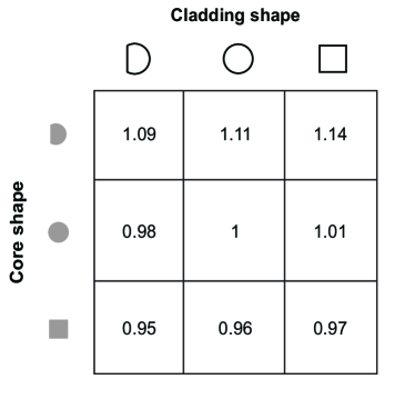
Figure 7: Relative slopes for linear scaling of TMI threshold with number of excited modes in fibers with various combinations of core and cladding shapes. The standard circular fiber (center) is normalized to 1. D-shaped core leads to higher slope than both circular and square shaped cores for each type of cladding. The highest slope in obtained when D-shaped core is combined with a square cladding, which leads to $14\%$ higher slope than the standard circular fiber.

In the fibers discussed so far, we consider the same shape for both core and cladding. The core shape determines the optical modes, and the cladding shape determines the temperature modes. Since the thermo-optical coupling coefficient depends on the overlap of optical and temperature modes, this suggests it may be possible to achieve a further reduction of TMI by studying fibers with different combinations of core and cladding shapes. To explore this we study 9 different fibers resulting from all combinations of 3 core shapes (D-shaped, circle, and square) and same 3 cladding shapes. We calculate the thermo-optical coupling matrices for all of these combinations, which are found to be banded matrices as expected. We also calculate the scaling of TMI threshold in each case and obtain a linear increase with the number of excited modes, with slightly different slopes. For a comparison, in Fig. 7, we show a table of relative slopes for the TMI threshold scaling with $M$ for all 9 fibers. The center which represents the slope for standard circular fiber is normalized to a value of 1. It can be seen the fibers with a D core shape have relatively higher slopes. Although the effect of the cladding shape on the slope is relatively weaker, the overall highest slope is obtained for a fiber with square cladding and D-shaped core. For this combination, the observed slope is roughly 14% higher than the standard circular fiber. A possible reason for the highest TMI threshold increase in case of the fiber with D-shaped core and square cladding is that this fiber supports optical modes which lack structure, but the temperature modes are highly structured, thus leading to relatively inefficient thermo-optical modal overlap and lower thermo-optical coupling. These results support the idea that custom designed non-circular fibers can enhance the TMI thresholds.

IV Discussion and Conclusion

In this work we have developed a theory of TMI, which can be used for efficient calculation of TMI threshold for arbitrary multimode excitations and fiber geometries. A key result obtained from this theory is that TMI threshold increases linearly with effective number of excited modes. The scaling is a result of the fundamentally diffusive nature of the heat propagation underlying the thermo-optical mode coupling. As such, it is expected to be applicable to a broad range of fibers. This opens up the use of highly multimode fibers as a promising avenue for instability-free power scaling in high-power fiber amplifiers.

A primary reason that multimode fibers have not found widespread use in high-power applications has been the generation of speckled internal fields due to both fiber dispersion and imperfections. There has been a general belief in this sub-field that the presence of multiple spatial modes necessarily leads to a poor output beam quality and a high value of $M^{2}$Zhan et al. (2009); Chu et al. (2019). However, this belief is not correct, as previous work on the manipulation of coherent optical fields has shown Florentin et al. (2017); Čižmár, Tomáš, and Dholakia (2011); Geng et al. (2021). Indeed the fields in multimode fibers can maintain a high output beam quality as long as the light remains sufficiently coherentSiegman (1993); Yoda, Polynkin, and Mansuripur (2006), i.e., the signal linewidth is narrower than the spectral correlation width of the fiber. In fact, a spatial light modulator (SLM) at either the fiber input or the output can be used to control the phases in various modes such that, after multimode propagation, the light is focused to a diffraction-limited spot outside the fiberGomes et al. (2022), and can then be collimated using a single lens. This process can be implemented with negligible loss by using two SLMs separated by free-space propagationJesacher et al. (2008). The ability to focus to a diffraction limited spot after multimode propagation has actually been demonstrated experimentally in both activeFlorentin et al. (2017) and passive fibersČižmár, Tomáš, and Dholakia (2011); Geng et al. (2021). Since focusing to diffraction-limited spot in the near field necessarily leads to excitation of multiple fiber modes, our theory predicts that it will lead to a higher TMI threshold than FM-only excitation, with a scaling proportional to the effective number of fiber modes. Hence the method just discussed can be used to increase the TMI threshold while maintaining good beam quality. A similar result was recently demonstrated experimentally for the case of Stimulated Brillouin Scattering (SBS) in multimode fibers; the threshold for the onset of SBS was demonstrated to increase significantly by focusing the output light of a multimode fiber to a diffraction-limited spotChen et al. (2023a).

To derive a tractable formula for the TMI threshold in the presence of multimode excitation, we have made a number of simplifying assumptions in our derivation. We have ignored any random linear mode couplingHo and Kahn (2011) in the fiber and assumed that the signal power in each mode grows independently. These assumptions can be relaxed relatively straightforwardly by numerically solving the equation for signal growth in the presence of random mode coupling instead of assuming an analytical solution as we did in Eq. 15, in which case, the integral in the formula for TMI gain (Eq. 20) needs to be evaluated numerically as well. As for the multimode TMI threshold, the presence of mode mixing is actually conducive to TMI suppression, since it promotes equipartition of signal power in various modesChen et al. (2023b). Here, we have also neglected both pump depletion and gain saturationDong (2022), and assumed a constant gain coefficient $g$. Gain saturation can be an especially important effect, since it is known to increase the TMI threshold by lowering the relevant heat loadHansen, Rymann, and Lægsgaard (2014); Smith and Smith (2013b); Dong (2022). Both the saturation and depletion effects can be added to our formalism by introducing coupled signal and pump equations, which can be solved numericallyLægaard (2020) as the first step in the modified calculation. Once the saturated signal is obtained, it can be used in Eq. 20 along with a modified thermo-optical coupling coefficient matrix (due to saturation of heat load) to calculate the TMI threshold for any input excitation. Solving coupled signal and pump equations with spatial hole-burning is a relatively computationally intensive process, especially for highly multimode excitations, as the equations would be coupled in both longitudinal and traverse directions. Since the primary focus in this paper is to elucidate the physics of multimode excitation on the TMI threshold, including the gain saturation has been deferred to future studies. These studies are in progress, and a manuscript including a full account of the effect of gain saturation on the TMI threshold for multimode excitations is in preparation. Our approach here is further justified by the fact that the key result of this paper, that the TMI threshold increases with the number of excited modes, follows from the diffusive nature of the heat equation, and is found to be robust to the inclusion of gain saturation.

Experimental validation of the theoretical results provided in this paper would be an important next step. Time-domain numerical simulations of optical and heat equations for up to 5 mode excitations in 1D cross-section waveguides are provided in ref. Chen et al. (2023b) and are in good agreement with our theory. Additionally, several recent experimental studies investigating the effect of fiber bending on the TMI threshold in few-mode fibers provide evidence for our predictionsZhang et al. (2019); Wen et al. (2022); Li et al. (2023). It has been observed that in a few-mode fiber, when the bend diameter of the fiber is increased (fiber being loosely coiled), a higher TMI threshold is obtained. For a large bend diameter, the bending loss of the HOMs decreases, thus the effective number of excited modes is higher, which leads to a higher TMI threshold in accordance with our predictions. In fact, the previous theories which only consider FM-only excitation predict that decreasing the HOM loss by increasing bend diameter should lead to lowering of the TMI threshold, in contrast to the experimental findingsDong (2023); Tao et al. (2016). This discrepancy is a result of ignoring the signal power in HOMs, which is fully taken into account in our theory. More systematic experimental studies are needed to investigate our predictions quantitatively.

In recent years, there has been a significant progress in fabricating low-loss fibers with non-circular cross-sectionsVelsink et al. (2021); Ying et al. (2017). These fibers have been proposed as a way to manipulate the strength of nonlinearitiesMorris et al. (2012). As noted above, the theory derived here can be used to calculate the TMI threshold for any fiber cross-section geometry. We utilized it to demonstrate that a D-shaped fiber performs better than a standard circular fiber in raising the TMI threshold via multimode excitation. This interplay between input excitation and fiber geometry can provide a number of avenues for manipulating the strength of nonlinearities in the fiber. We believe that our theory can be utilized as a framework for customizing the strength of the thermo-optical nonlinearity using optimized fiber designs He et al. (2020). Although in this work only step-index fibers have been discussed, our theory and key results should be applicable in fibers with other refractive index profiles such as graded index fibers. We expect the linear scaling of the TMI threshold to be maintained, but, consistent with our finding here, with a slope depending on the specific refractive index profile. Utilizing the spatial degrees of freedom of the fields to control nonlinear effects is becoming a standard tool, and has been demonstrated for diverse effects such as SBSChen et al. (2023a); Wisal et al. (2023, 2022), stimulated Raman scattering (SRS)Tzang et al. (2018), and Kerr nonlinearityWright, Christodoulides, and Wise (2015); Krupa et al. (2017). Our work contributes to this exciting area by bringing the thermo-optical nonlinearity, with its different physical origin, into this category and at the same time providing a solution to the practical challenge of TMI suppression.

author declaration

The authors declare no conflict of interest.

References

- Even and Pureur (2002) P. Even and D. Pureur, “High-power double-clad fiber lasers: a review,” Optical Devices for Fiber Communication III 4638, 1–12 (2002).
- Jeong et al. (2004) Y. e. Jeong, J. Sahu, D. Payne, , and J. Nilsson, “Ytterbium-doped large-core fiber laser with 1.36 kW continuous-wave output power,” Optics Express 12, 6088–6092 (2004).
- Nilsson and Payne (2011) J. Nilsson and D. N. Payne, “High-power fiber lasers,” Science 332, 921–922 (2011).
- Jauregui, Limpert, and Tünnermann (2013) C. Jauregui, J. Limpert, and A. Tünnermann, “High-power fibre lasers,” Nature Photonics 7, 861–867 (2013).
- Zervas and Codemard (2013) M. N. Zervas and C. A. Codemard, “High Power Fiber Lasers: A Review,” IEEE Journal of Selected Topics in Quantum Electronics 20, 0904123 (2013).
- Dong and Samson (2016) L. Dong and B. Samson, Fiber lasers: basics, technology, and applications (CRC press, 2016).
- Kawahito et al. (2018) Y. Kawahito, H. Wang, S. Katayama, and D. Sumimori, “Ultra high power (100 kW) fiber laser welding of steel,” Optics Letters 43, 4667–4670 (2018).
- Buikema et al. (2019) A. Buikema, F. Jose, S. J. Augst, P. Fritschel, and N. Mavalvala, “Narrow-linewidth fiber amplifier for gravitational-wave detectors,” Optics Letters 44, 3833–3836 (2019).
- Ludewigt et al. (2019) K. Ludewigt, A. Liem, U. Stuhr, and M. Jung, “High-power laser development for laser weapons,” in Proc. SPIE 11162, High Power Lasers: Technology and Systems, Platforms, Effects III (2019) p. 1116207.
- Dawson et al. (2008) J. W. Dawson, M. J. Messerly, R. J. Beach, M. Y. Shverdin, E. A. Stappaerts, A. K. Sridharan, P. H. Pax, J. E. Heebner, C. W. Siders, and C. Barty, “Analysis of the scalability of diffraction-limited fiber lasers and amplifiers to high average power,” Optics Express 16, 13240–13266 (2008).
- Jauregui, Stihler, and Limpert (2020) C. Jauregui, C. Stihler, and J. Limpert, “Transverse mode instability,” Advances in Optics and Photonics 12, 429–484 (2020).
- Eidam et al. (2011a) T. Eidam, C. Wirth, C. Jauregui, F. Stutzki, F. Jansen, H.-J. Otto, O. Schmidt, T. Schreiber, J. Limpert, and A. Tünnermann, “Experimental observations of the threshold-like onset of mode instabilities in high power fiber amplifiers,” Optics Express 19, 13218–13224 (2011a).
- Smith and Smith (2011) A. V. Smith and J. J. Smith, “Mode instability in high power fiber amplifiers,” Optics Express 19, 10180–10192 (2011).
- Ward, Robin, and Dajani (2012) B. Ward, C. Robin, and I. Dajani, “Origin of thermal modal instabilities in large mode area fiber amplifiers,” Optics Express 20, 11407–11422 (2012).
- Boyd (2020) R. W. Boyd, Nonlinear optics (Academic press, 2020).
- Kobyakov, Sauer, and Chowdhury (2010) A. Kobyakov, M. Sauer, and D. Chowdhury, “Stimulated brillouin scattering in optical fibers,” Advances in optics and photonics 2, 1–59 (2010).
- Wolff et al. (2021) C. Wolff, M. Smith, B. Stiller, and C. Poulton, “Brillouin scattering—theory and experiment: tutorial,” JOSA B 38, 1243–1269 (2021).
- Hansen et al. (2013) K. R. Hansen, T. T. Alkeskjold, J. Broeng, and J. Lægsgaard, “Theoretical analysis of mode instability in high-power fiber amplifiers,” Optics Express 21, 1944–1971 (2013).
- Dong (2013) L. Dong, “Stimulated thermal rayleigh scattering in optical fibers,” Optics Express 21, 2642–2656 (2013).
- Ward (2013) B. G. Ward, “Modeling of transient modal instability in fiber amplifiers,” Optics Express 21, 12053–12067 (2013).
- Ward (2016) B. Ward, “Theory and modeling of photodarkening-induced quasi static degradation in fiber amplifiers,” Optics Express 24, 3488–3501 (2016).
- Zervas (2019) M. N. Zervas, “Transverse-modal-instability gain in high power fiber amplifiers: Effect of the perturbation relative phase,” APL Photonics 4, 022802 (2019).
- Jauregui et al. (2011) C. Jauregui, T. Eidam, J. Limpert, and A. Tünnermann, “Impact of modal interference on the beam quality of high-power fiber amplifiers,” Optics Express 19, 3258–3271 (2011).
- Jauregui et al. (2012) C. Jauregui, T. Eidam, H.-J. Otto, F. Stutzki, F. Jansen, J. Limpert, and A. Tünnermann, “Physical origin of mode instabilities in high-power fiber laser systems,” Optics Express 20, 12912–12925 (2012).
- Otto et al. (2012) H.-J. Otto, F. Stutzki, F. Jansen, T. Eidam, C. Jauregui, J. Limpert, and A. Tünnermann, “Temporal dynamics of mode instabilities in high-power fiber lasers and amplifiers,” Optics Express 20, 15710–15722 (2012).
- Naderi et al. (2013) S. Naderi, I. Dajani, T. Madden, and C. Robin, “Investigations of modal instabilities in fiber amplifiers through detailed numerical simulations,” Optics Express 21, 16111–16129 (2013).
- Kuznetsov et al. (2014) M. Kuznetsov, O. Vershinin, V. Tyrtyshnyy, and O. Antipov, “Low-threshold mode instability in yb 3+-doped few-mode fiber amplifiers,” Optics Express 22, 29714–29725 (2014).
- Kong et al. (2016) F. Kong, J. Xue, R. H. Stolen, and L. Dong, “Direct experimental observation of stimulated thermal rayleigh scattering with polarization modes in a fiber amplifier,” Optica 3, 975–978 (2016).
- Stihler et al. (2018) C. Stihler, C. Jauregui, A. Tünnermann, and J. Limpert, “Modal energy transfer by thermally induced refractive index gratings in yb-doped fibers,” Light: Science & Applications 7, 1–12 (2018).
- Stihler et al. (2020) C. Stihler, C. Jauregui, S. E. Kholaif, and J. Limpert, “Intensity noise as a driver for transverse mode instability in fiber amplifiers,” PhotoniX 1, 1–17 (2020).
- Menyuk et al. (2021) C. R. Menyuk, J. T. Young, J. Hu, A. J. Goers, D. M. Brown, and M. L. Dennis, “Accurate and efficient modeling of the transverse mode instability in high energy laser amplifiers,” Optics Express 29, 17746–17757 (2021).
- Chu et al. (2021) Q. Chu, C. Guo, X. Yang, F. Li, D. Yan, H. Zhang, and R. Tao, “Increasing mode instability threshold by mitigating driver noise in high power fiber amplifiers,” IEEE Photonics Technology Letters 33, 1515–1518 (2021).
- Ren et al. (2022) S. Ren, W. Lai, G. Wang, W. Li, J. Song, Y. Chen, P. Ma, W. Liu, and P. Zhou, “Experimental study on the impact of signal bandwidth on the transverse mode instability threshold of fiber amplifiers,” Optics Express 30, 7845–7853 (2022).
- Otto et al. (2013) H.-J. Otto, C. Jauregui, F. Stutzki, F. Jansen, J. Limpert, and A. Tünnermann, “Controlling mode instabilities by dynamic mode excitation with an acousto-optic deflector,” Optics Express 21, 17285–17298 (2013).
- Hawkins et al. (2021) T. W. Hawkins, P. D. Dragic, N. Yu, A. Flores, M. Engholm, and J. Ballato, “Kilowatt power scaling of an intrinsically low Brillouin and thermo-optic Yb-doped silica fiber [Invited],” Journal of the Optical Society of America B 38, F38–F49 (2021).
- Dong, Ballato, and Kolis (2023) L. Dong, J. Ballato, and J. Kolis, “Power scaling limits of diffraction-limited fiber amplifiers considering transverse mode instability,” Optics Express 31, 6690–6703 (2023).
- Tao et al. (2015a) R. Tao, P. Ma, X. Wang, P. Zhou, and Z. Liu, “Mitigating of modal instabilities in linearly-polarized fiber amplifiers by shifting pump wavelength,” Journal of Optics 17, 045504 (2015a).
- Jauregui et al. (2018) C. Jauregui, C. Stihler, A. Tünnermann, and J. Limpert, “Pump-modulation-induced beam stabilization in high-power fiber laser systems above the mode instability threshold,” Optics express 26, 10691–10704 (2018).
- Stutzki et al. (2011) F. Stutzki, F. Jansen, T. Eidam, A. Steinmetz, C. Jauregui, J. Limpert, and A. Tünnermann, “High average power large-pitch fiber amplifier with robust single-mode operation,” Optics letters 36, 689–691 (2011).
- Eidam et al. (2011b) T. Eidam, S. Hädrich, F. Jansen, F. Stutzki, J. Rothhardt, H. Carstens, C. Jauregui, J. Limpert, and A. Tünnermann, “Preferential gain photonic-crystal fiber for mode stabilization at high average powers,” Optics Express 19, 8656–8661 (2011b).
- Jauregui et al. (2013) C. Jauregui, H.-J. Otto, F. Stutzki, F. Jansen, J. Limpert, and A. Tünnermann, “Passive mitigation strategies for mode instabilities in high-power fiber laser systems,” Optics Express 21, 19375–19386 (2013).
- Robin, Dajani, and Pulford (2014) C. Robin, I. Dajani, and B. Pulford, “Modal instability-suppressing, single-frequency photonic crystal fiber amplifier with 811 W output power,” Optics Letters 39, 666–669 (2014).
- Haarlammert et al. (2015) N. Haarlammert, B. Sattler, A. Liem, M. Strecker, J. Nold, T. Schreiber, R. Eberhardt, A. Tünnermann, K. Ludewigt, and M. Jung, “Optimizing mode instability in low-na fibers by passive strategies,” Optics letters 40, 2317–2320 (2015).
- Tao et al. (2016) R. Tao, R. Su, P. Ma, X. Wang, and P. Zhou, “Suppressing mode instabilities by optimizing the fiber coiling methods,” Laser Physics Letters 14, 025101 (2016).
- Otto et al. (2014) H.-J. Otto, A. Klenke, C. Jauregui, F. Stutzki, J. Limpert, and A. Tünnermann, “Scaling the mode instability threshold with multicore fibers,” Optics Letters 39, 2680–2683 (2014).
- Klenke et al. (2022) A. Klenke, C. Jauregui, A. Steinkopff, C. Aleshire, and J. Limpert, “High-power multicore fiber laser systems,” Progress in Quantum Electronics , 100412 (2022).
- Abedin et al. (2012) K. Abedin, T. Taunay, M. Fishteyn, D. DiGiovanni, V. Supradeepa, J. Fini, M. Yan, B. Zhu, E. Monberg, and F. Dimarcello, “Cladding-pumped erbium-doped multicore fiber amplifier,” Optics express 20, 20191–20200 (2012).
- Hansen et al. (2011) K. R. Hansen, T. T. Alkeskjold, J. Broeng, and J. Lægsgaard, “Thermo-optical effects in high-power ytterbium-doped fiber amplifiers,” Optics express 19, 23965–23980 (2011).
- Zhan et al. (2009) Y. Zhan, Q. Yang, H. Wu, J. Lei, and P. Liang, “Degradation of beam quality and depolarization of the laser beam in a step-index multimode optical fiber,” Optik 120, 585–590 (2009).
- Chu et al. (2019) Q. Chu, R. Tao, C. Li, H. Lin, Y. Wang, C. Guo, J. Wang, F. Jing, and C. Tang, “Experimental study of the influence of mode excitation on mode instability in high power fiber amplifier,” Scientific Reports 9, 1–7 (2019).
- Florentin et al. (2017) R. Florentin, V. Kermene, J. Benoist, A. Desfarges-Berthelemot, D. Pagnoux, A. Barthélémy, and J.-P. Huignard, “Shaping the light amplified in a multimode fiber,” Light: Science & Applications 6, e16208 (2017).
- Geng et al. (2021) Y. Geng, H. Chen, Z. Zhang, B. Zhuang, H. Guo, Z. He, and D. Kong, “High-speed focusing and scanning light through a multimode fiber based on binary phase-only spatial light modulation,” Applied Physics B 127, 1–6 (2021).
- Leite et al. (2018) I. T. Leite, S. Turtaev, X. Jiang, M. Šiler, A. Cuschieri, P. S. J. Russell, and T. Čižmár, “Three-dimensional holographic optical manipulation through a high-numerical-aperture soft-glass multimode fibre,” Nature Photonics 12, 33–39 (2018).
- Gomes et al. (2022) A. D. Gomes, S. Turtaev, Y. Du, and T. Čižmár, “Near perfect focusing through multimode fibres,” Optics Express 30, 10645–10663 (2022).
- Teğin et al. (2020) U. Teğin, B. Rahmani, E. Kakkava, N. Borhani, C. Moser, and D. Psaltis, “Controlling spatiotemporal nonlinearities in multimode fibers with deep neural networks,” Apl Photonics 5, 030804 (2020).
- Wright, Christodoulides, and Wise (2015) L. G. Wright, D. N. Christodoulides, and F. W. Wise, “Controllable spatiotemporal nonlinear effects in multimode fibres,” Nature photonics 9, 306–310 (2015).
- Krupa et al. (2019) K. Krupa, A. Tonello, A. Barthélémy, T. Mansuryan, V. Couderc, G. Millot, P. Grelu, D. Modotto, S. A. Babin, and S. Wabnitz, “Multimode nonlinear fiber optics, a spatiotemporal avenue,” APL Photonics 4, 110901 (2019).
- Qiu et al. (2023) T. Qiu, H. Cao, K. Liu, E. Lendaro, F. Wang, and S. You, “Spatiotemporal control of nonlinear effects in multimode fibers for two-octave high-peak-power femtosecond tunable source,” arXiv preprint arXiv:2306.05244 (2023).
- Wisal et al. (2022) K. Wisal, S. C. Warren-Smith, C.-W. Chen, R. Behunin, H. Cao, and A. D. Stone, “Generalized theory of SBS in multimode fiber amplifiers,” in Physics and Simulation of Optoelectronic Devices XXX (SPIE, 2022) p. PC1199504.
- Wisal et al. (2023) K. Wisal, S. C. Warren-Smith, C.-W. Chen, H. Cao, and A. D. Stone, “Theory of stimulated brillouin scattering in fibers for highly multimode excitations,” arXiv preprint arXiv:2304.09342 (2023).
- Chen et al. (2023a) C.-W. Chen, L. V. Nguyen, K. Wisal, S. Wei, S. C. Warren-Smith, O. Henderson-Sapir, E. P. Schartner, P. Ahmadi, H. Ebendorff-Heidepriem, A. D. Stone, et al., “Mitigating stimulated brillouin scattering in multimode fibers with focused output via wavefront shaping,” arXiv preprint arXiv:2305.02534 (2023a).
- Tzang et al. (2018) O. Tzang, A. M. Caravaca-Aguirre, K. Wagner, and R. Piestun, “Adaptive wavefront shaping for controlling nonlinear multimode interactions in optical fibres,” Nature Photonics 12, 368–374 (2018).
- Chen et al. (2023b) C.-W. Chen, K. Wisal, Y. Eliezer, A. D. Stone, and H. Cao, “Suppressing transverse mode instability through multimode excitation in a fiber amplifier,” Proceedings of the National Academy of Sciences 120, e2217735120 (2023b).
- Smith and Smith (2013a) A. V. Smith and J. J. Smith, “Steady-periodic method for modeling mode instability in fiber amplifiers,” Optics Express 21, 2606–2623 (2013a).
- Smith and Smith (2013b) A. V. Smith and J. J. Smith, “Increasing mode instability thresholds of fiber amplifiers by gain saturation,” Optics Express 21, 15168–15182 (2013b).
- Hansen, Rymann, and Lægsgaard (2014) Hansen, K. Rymann, and J. Lægsgaard, “Impact of gain saturation on the mode instability threshold in high-power fiber amplifiers,” Optics Express 22, 11267–11278 (2014).
- Tao et al. (2015b) R. Tao, P. Ma, X. Wang, P. Zhou, and Z. Liu, “Study of wavelength dependence of mode instability based on a semi-analytical model,” IEEE Journal of quantum electronics 51, 1–6 (2015b).
- Jauregui et al. (2015) C. Jauregui, H.-J. Otto, F. Stutzki, J. Limpert, and A. Tünnermann, “Simplified modelling the mode instability threshold of high power fiber amplifiers in the presence of photodarkening,” Optics Express 23, 20203–20218 (2015).
- Zervas (2017) M. N. Zervas, “Transverse mode instability analysis in fiber amplifiers,” in Fiber Lasers XIV: Technology and Systems, Vol. 10083 (SPIE, 2017) pp. 115–123.
- Tao, Wang, and Zhou (2018) R. Tao, X. Wang, and P. Zhou, “Comprehensive theoretical study of mode instability in high-power fiber lasers by employing a universal model and its implications,” IEEE Journal of Selected Topics in Quantum Electronics 24, 1–19 (2018).
- Dong (2022) L. Dong, “Accurate modeling of transverse mode instability in fiber amplifiers,” Journal of Lightwave Technology 40, 4795 – 4803 (2022).
- Cronin-Golomb et al. (1984) M. Cronin-Golomb, B. Fischer, J. White, and A. Yariv, “Theory and applications of four-wave mixing in photorefractive media,” IEEE Journal of Quantum Electronics 20, 12–30 (1984).
- Okamoto (2021) K. Okamoto, Fundamentals of optical waveguides (Elsevier, 2021).
- Snyder and Young (1978) A. W. Snyder and W. R. Young, “Modes of optical waveguides,” JOSA 68, 297–309 (1978).
- (75) “Comsol multiphysics v. 5.5. www.comsol.com. comsol ab, stockholm, sweden,” .
- Marcatili (1969) E. A. Marcatili, “Dielectric rectangular waveguide and directional coupler for integrated optics,” Bell System Technical Journal 48, 2071–2102 (1969).
- Bittner et al. (2020) S. Bittner, K. Kim, Y. Zeng, Q. J. Wang, and H. Cao, “Spatial structure of lasing modes in wave-chaotic semiconductor microcavities,” New Journal of Physics 22, 083002 (2020).
- Cole et al. (2010) K. Cole, J. Beck, A. Haji-Sheikh, and B. Litkouhi, Heat conduction using Greens functions (Taylor & Francis, 2010).
- Sun, Zhang, and Gao (2023) Z.-Z. Sun, Q. Zhang, and G.-h. Gao, Finite difference methods for nonlinear evolution equations, Vol. 8 (Walter de Gruyter GmbH & Co KG, 2023).
- Qian and Huang (1986) J.-R. Qian and W.-p. Huang, “Lp modes and ideal modes on optical fibers,” Journal of lightwave technology 4, 626–630 (1986).
- Seyf and Henry (2016) H. R. Seyf and A. Henry, “A method for distinguishing between propagons, diffusions, and locons,” Journal of Applied Physics 120 (2016).
- Zhang et al. (2019) F. Zhang, H. Xu, Y. Xing, S. Hou, Y. Chen, J. Li, N. Dai, H. Li, Y. Wang, and L. Liao, “Bending diameter dependence of mode instabilities in multimode fiber amplifier,” Laser Physics Letters 16, 035104 (2019).
- Wen et al. (2022) Y. Wen, P. Wang, C. Shi, B. Yang, X. Xi, H. Zhang, and X. Wang, “Experimental study on transverse mode instability characteristics of few-mode fiber laser amplifier under different bending conditions,” IEEE Photonics Journal 14, 1–6 (2022).
- Li et al. (2023) R. Li, H. Li, H. Wu, H. Xiao, J. Leng, L. Huang, Z. Pan, and P. Zhou, “Mitigation of tmi in an 8 kw tandem pumped fiber amplifier enabled by inter-mode gain competition mechanism through bending control,” Optics Express 31, 24423–24436 (2023).
- Dong (2023) L. Dong, “Transverse mode instability considering bend loss and heat load,” Optics Express 31, 20480–20488 (2023).
- Velsink et al. (2021) M. C. Velsink, Z. Lyu, P. W. Pinkse, and L. V. Amitonova, “Comparison of round-and square-core fibers for sensing, imaging, and spectroscopy,” Optics express 29, 6523–6531 (2021).
- Ying et al. (2017) Y. Ying, G.-y. Si, F.-j. Luan, K. Xu, Y.-w. Qi, and H.-n. Li, “Recent research progress of optical fiber sensors based on d-shaped structure,” Optics & laser technology 90, 149–157 (2017).
- Bittner et al. (2018) S. Bittner, S. Guazzotti, Y. Zeng, X. Hu, H. Yılmaz, K. Kim, S. S. Oh, Q. J. Wang, O. Hess, and H. Cao, “Suppressing spatiotemporal lasing instabilities with wave-chaotic microcavities,” Science 361, 1225–1231 (2018).
- Redding et al. (2015) B. Redding, A. Cerjan, X. Huang, M. L. Lee, A. D. Stone, M. A. Choma, and H. Cao, “Low spatial coherence electrically pumped semiconductor laser for speckle-free full-field imaging,” Proceedings of the National Academy of Sciences 112, 1304–1309 (2015).
- Čižmár, Tomáš, and Dholakia (2011) Čižmár, Tomáš, and K. Dholakia, “Shaping the light transmission through a multimode optical fibre: complex transformation analysis and applications in biophotonics,” Optics Express 19, 18871–18884 (2011).
- Siegman (1993) A. E. Siegman, “Defining, measuring, and optimizing laser beam quality,” Laser Resonators and Coherent Optics: Modeling, Technology, and Applications 1868, 2–12 (1993).
- Yoda, Polynkin, and Mansuripur (2006) H. Yoda, P. Polynkin, and M. Mansuripur, “Beam quality factor of higher order modes in a step-index fiber,” Journal of lightwave technology 24, 1350–1355 (2006).
- Jesacher et al. (2008) A. Jesacher, C. Maurer, A. Schwaighofer, S. Bernet, and M. Ritsch-Marte, “Near-perfect hologram reconstruction with a spatial light modulator,” Optics Express 16, 2597–2603 (2008).
- Ho and Kahn (2011) K.-P. Ho and J. M. Kahn, “Mode-dependent loss and gain: statistics and effect on mode-division multiplexing,” Optics express 19, 16612–16635 (2011).
- Lægaard (2020) J. Lægaard, “Multimode nonlinear simulation technique having near-linear scaling with mode number in circular symmetric waveguides,” Optics Letters 45, 4160–4163 (2020).
- Morris et al. (2012) S. Morris, C. McMillen, T. Hawkins, P. Foy, R. Stolen, J. Ballato, and R. Rice, “The influence of core geometry on the crystallography of silicon optical fiber,” Journal of crystal growth 352, 53–58 (2012).
- He et al. (2020) Z. He, J. Du, X. Chen, W. Shen, Y. Huang, C. Wang, K. Xu, and Z. He, “Machine learning aided inverse design for few-mode fiber weak-coupling optimization,” Optics Express 28, 21668–21681 (2020).
- Krupa et al. (2017) K. Krupa, A. Tonello, B. Shalaby, M. Fabert, A. Barthélémy, G. Millot, S. Wabnitz, and V. Couderc, “Spatial beam self-cleaning in multimode fibres,” Nature Photonics 11, 237–241 (2017).