Cosmic acceleration in Lovelock quantum gravity

Abstract

This paper introduces novel solutions for inflation and late-time cosmic acceleration within the framework of quantum Lovelock gravity, utilizing Friedmann equations. Furthermore, we demonstrate the hypergeometric states of cosmic acceleration through the Schrödinger stationary equation. A physical interpretation is proposed, whereby the rescaled Lovelock couplings represent a topological mass that characterizes the Lovelock branch. This research holds the potential for an extension into the quantum description. Predictions for the spectral tilt and tensor-to-scalar ratio are depicted through plotted curves. By utilizing the rescaled Hubble parameter, the spectral index is determined in terms of the number of e-folds.

1 Introduction

Lovelock gravity [1] represents a generalization of Einstein’s theory of general relativity to higher dimensions within the realm of higher curvature gravity theories. Several aspects of Lovelock theories in general dimensions are studied in [2, 3, 4, 5, 6], particularly, the thermodynamic properties of the Lovelock black hole [7, 8, 9, 10, 11, 12]. The articles [13, 14, 15] focused on investigating the third-order Lovelock gravity with black holes. Additionally, there exist other studies examining the connection between Lovelock gravity and various theories, including Lanczos-Lovelock [16, 17], Lovelock-Cartan theory [18], AdS/CFT [19], and Horndeski theories [20]. In [21], the gravitational field of Lovelock was investigated within the context of cosmology. The Friedmann equations are a set of equations that describe the evolution of the universe on a large scale [22, 23]. In Lovelock gravity, the Friedmann equations are modified to include additional terms that arise from the higher-dimensional nature of the theory [24, 25]. Recent progress in quantum Friedmann equations offers a promising framework for generating new solutions for cosmic acceleration, as mentioned in [26, 28, 32]. The cosmological Friedman-Einstein dynamical system can be reformulated as a type of Schrödinger equation, where the bound eigensolutions correspond to oscillating functions [29]. In quantum gravity, the customary approach involves treating the entire universe as a quantum system [33, 34]. This perspective often entails considering multiple co-existing and non-interacting universes. The Wheeler-DeWitt equation $\hat{H}\psi=0$, governing the wave function of the universe $\psi$, can be expressed as a Schrödinger equation within the Friedman-Robertson-Walker (FRW) spacetime. The article [35] discusses an inflationary model that is based on Lovelock’s terms. These terms involve higher-order curvature and can cause inflation to occur when there are more than three spatial dimensions.
This study aims to find an interpretation of cosmic expansion following a connection between Lovelock gravity and quantum mechanics by examining the energy states of cosmic expansion in terms of Lovelock coupling.
The structure of this paper is outlined as follows: Section 2 delves into the examination of the Friedmann equations within Lovelock gravity, as well as the exploration of topological density. In section 3, we study the cosmic acceleration from quantum states derived by the FRW-Lovelock universe and Schrödinger stationary equation through the Hubble parameter reparameterization. In section 4, we study the cosmic expansion according to Schrödinger equation and we examine our proposal in various different hypergeometric states. In Section 5, we analyze the observational constraints on Lovelock inflation. Finally, section 6 concludes the paper by summarizing our findings. Throughout this article, we use units $c=\hbar=k_{B}=1$.

2 General Lovelock gravity

Let us start with the Lagrangian of the $(D+1)$-dimensional Lovelock gravity [1] of extended Euler densities is given by

$$\mathcal{L}=\sum_{k=0}^{\bar{D}}\frac{\alpha_{k}}{16\pi G_{N}}2^{-k}\delta_{c_{1}d_{1}\cdots c_{k}d_{k}}^{a_{1}b_{1}\cdots a_{k}b_{k}}R_{a_{1}b_{1}}^{\text{ \ \ \ \ }c_{1}d_{1}}\ldots R_{a_{k}b_{k}}^{\text{ \ \ \ \ }c_{k}d_{k}}+\mathcal{L}_{m},$$ (2.1)

where $L_{m}$ is the matter Lagrangian, $\bar{D}=\left[\frac{D-1}{2}\right]$ (the brackets $\left[\cdots\right]$ denote taking the integer part), $\delta_{c_{1}d_{1}\cdots c_{k}d_{k}}^{a_{1}b_{1}\cdots a_{k}b_{k}}$ is the generalized antisymmetric Kronecker delta and $R_{a_{1}b_{1}}^{\text{ \ \ \ \ }c_{1}d_{1}}$ is the Riemann tensor. We notice that $\alpha_{k}$ are the Lovelock coupling constants with dimensions $(length)^{2k-D}$, where D is the respective dimension. Here, $\alpha_{2}=\alpha\$and $\alpha_{3}$ are respectively the second (Gauss-Bonnet coupling [36, 37]) and the third Lovelock coefficients. The zero-order Lovelock invariant is $\alpha_{0}L_{0}=-2\Lambda=\frac{\left(D-1\right)\left(D-2\right)}{L^{2}}$ with $\Lambda$ being the cosmological constant and $L$ is the AdS radius [54]. The first-order Lovelock invariant is $\alpha_{1}L_{1}=R$ is the Einstein-Hilbert Lagrangian. The equations of motion for Lovelock gravity [38, 39] read

$$\sum_{k=0}^{\bar{D}}\frac{\alpha_{k}}{16\pi G_{N}}2^{-2k-1}\delta_{\mathbf{a}a_{1}b_{1}\cdots a_{k}b_{k}}^{\mathbf{b}c_{1}d_{1}\cdots c_{k}d_{k}}R_{c_{1}d_{1}}^{\text{ \ \ \ \ }a_{1}b_{1}}\ldots=T_{a}^{b}\mathbf{,}$$ (2.2)

where $T_{a}^{b}$ is the stress tensor. Hence, by varying the Euler density [65], the stress tensor in a conformally flat background can be derived as

$$\left\langle T_{b}^{\text{ \ }a}\right\rangle=-\frac{C_{D}}{\left(-8\pi\right)^{\frac{D}{2}}}\lim_{n\rightarrow D}\frac{1}{n-D}R_{\text{ \ \ \ }a_{1}a_{2}}^{b_{1}b_{2}}\cdots R_{\text{ \ \ \ }a_{D-1}a_{D}}^{b_{D-1}b_{D}}\delta_{b_{1}\cdots b_{D}b}^{a_{1}\cdots a_{D}a},$$ (2.3)

where $C_{D}$ are the central charges. The $\left(D+1\right)$-dimensional FRW universe with the metric

$$ds^{2}=-dt^{2}+a^{2}(t)\left(\frac{dr^{2}}{1-\kappa r^{2}}+r^{2}d\Omega_{D-1}^{2}\right),$$ (2.4)

where $d\Omega_{D-1}^{2}$ denotes the line element of an $(D-1)$-dimensional unit sphere. The curvature parameter $\kappa$ can take the values $\kappa=+1$, $-1$, or $0$, corresponding to closed, open, or flat universes, respectively. The effective cosmological constant and energy density are modified in Lovelock gravity due to the presence of higher-dimensional terms. The pressure $p$ is related to the energy density and the equation of state of the matter and energy in the universe. In Lovelock gravity, it is modified by higher-dimensional terms. The continuity equation of the perfect fluid is given,

$$\dot{\rho}+HD\left(\rho+p\right)=0,$$ (2.5)

where $H=\frac{\dot{a}}{a}$ denotes the Hubble parameter and $a\left(t\right)$ is the scale factor that describes the relative expansion of the Universe. We introduce the coefficients $c_{k}$ are given by [24]

$$c_{0} = \frac{\alpha_{0}}{16\pi G_{N}}\frac{1}{D\left(D-1\right)}\text{,}$$ (2.6)

$$c_{1} = 1,$$

$$c_{k} = \frac{\alpha_{k}}{16\pi G_{N}}\prod\limits_{i=3}^{2\bar{D}}\left(D+1-i\right)\text{ for }i>1.$$

We assume that the entropy of the FRW universe follows the entropy

$$S=\frac{A}{4G_{N}}\sum_{n=1}^{\bar{D}}c_{k}\frac{n\left(D-1\right)}{D-2n+1}r_{A}^{2-2n}.$$ (2.7)

For apparent horizon [24, 41].Therefore, the radius of the black hole horizon is substituted with the radius of the apparent horizon [39] as

$$r_{A}=\left(H^{2}+\frac{\kappa}{a^{2}}\right)^{-\frac{1}{2}}.$$ (2.8)

We consider the entropy of the apparent horizon in the FRW universe, represented by Eq. (2.7). The temperature of the apparent horizon is written as [27]

$$T=-\frac{\kappa}{2\pi r_{A}}+\frac{\left(D-1\right)r_{A}}{4\pi\bar{D}\left(\frac{\kappa}{r_{A}^{2}}+\left(\bar{D}\alpha\right)^{-\frac{1}{\bar{D}-1}}\right)^{\bar{D}-1}}\left(\left(\frac{\kappa}{r_{A}^{2}}+\left(\bar{D}\alpha\right)^{-\frac{1}{\bar{D}-1}}\right)^{\bar{D}}-\left(\bar{D}\alpha\right)^{-\frac{\bar{D}}{\bar{D}-1}}+\frac{\alpha_{0}}{\alpha}\right).$$ (2.9)

We consider the standard perfect fluid matter, and apply the first law, $dM=TdS$, so that the Klein-Gordon equation can then be written from the metric function Eq. (2.4) [24] as

$$\sum_{n=1}^{\bar{D}}nc_{n}\left(H^{2}+\frac{\kappa}{a^{2}}\right)^{n-1}\left(\dot{H}-\frac{\kappa}{a^{2}}\right)=-\frac{8\pi G_{N}}{D-1}\left(\rho+p\right).$$ (2.10)

Using the continuity Eq. (2.5) and integrating Eq. (2.10), we finally obtain the Friedmann equation in the Lovelock gravity,

$$\sum_{n=1}^{\bar{D}}c_{n}\left(H^{2}+\frac{\kappa}{a^{2}}\right)^{n}=\frac{16\pi G_{N}}{D\left(D-1\right)}\rho.$$ (2.11)

The Friedmann equations in Lovelock gravity provide a framework for understanding the evolution of the universe in higher-dimensional theories of gravity. These equations can be used to study the behavior of the universe on large scales and to test the predictions of Lovelock gravity against observational data. When $\bar{D}=2$, Eqs. (2.10)-(2.11) reduce to those of the Gauss-Bonnet gravity:

$$\left(1+2\alpha\left(D-2\right)\left(D-3\right)\left(H^{2}+\frac{\kappa}{a^{2}}\right)\right)\left(\dot{H}-\frac{\kappa}{a^{2}}\right)$$

$$= -\frac{8\pi G_{N}}{\left(D-1\right)}\left(\rho+p\right),$$

$$H^{2}+\frac{\kappa}{a^{2}}+\alpha\left(D-2\right)\left(D-3\right)\left(H^{2}+\frac{\kappa}{a^{2}}\right)^{2}$$

$$= \frac{16\pi G_{N}}{D\left(D-1\right)}\rho.$$

If $\alpha=0$ or $D=3$, we get the standard form of the Friedmann equation. The Friedmann equations in Lovelock gravity can be used to study the evolution of the universe during the inflationary period and cosmic acceleration.

3 Topological cosmic acceleration

The effective energy density and pressure of the scalar field are modified due to the presence of higher-dimensional terms. The scalar field potential is also modified, which can affect the dynamics of the inflationary period and the production of primordial gravitational waves. According to the Einstein-scalar-Gauss-Bonnet gravity, the scalar field can play the role of Gauss-Bonnet coupling. In the general framework, we can always replace the Lovelock coupling with a scalar field [2]. The Brans-Dicke theory offers a potential explanation for the current accelerated expansion of the universe, eliminating the need for a cosmological constant or quintessence matter [42]. The topics of curvature quintessence and cosmic acceleration can be addressed within frameworks that do not necessarily involve scalar fields [43, 44]. We recall that the deceleration parameter is $q=-1-\frac{\dot{H}}{H^{2}}$. The accelerated behavior is achieved if $q<0$. The deceleration parameter can be given in terms of density $\rho$. First, for comparison, introducing a new reparameterization in the Lovelock gravity framework: $\sigma=1+\frac{\kappa}{a^{2}H^{2}}$. The parameter $\sigma$ is described by the curvature parameter $\kappa$. Using the conformal time $\tau=\sqrt{\sigma}t$, i.e. $\frac{\partial a}{a\partial t}=\sqrt{\sigma}\frac{\partial a}{a\partial\tau}$, which can be used to set $H=\frac{\partial a}{a\partial\tau}$, so the Hubble parameter simplifies to $H^{2}=\sigma H^{2}$. First, for comparison, introducing a new reparameterization of Hubble parameter and Lovelock couplings:

$$\mathcal{H}^{2} = \sigma H^{2}=H^{2}+\frac{\kappa}{a^{2}},$$ (3.1)

$$g_{n}^{2} = \frac{D\left(D-1\right)}{16\pi G_{N}}c_{n}.$$

The recent puzzle surrounding the variation in measured values of the Hubble rate, as observed by the Hubble Space Telescope and the Planck satellite, adds an intriguing aspect to this topic [45]. This gives the Hubble parameter great importance for our study, as a free parameter that generates all the differential equations thereafter. Second, we express the two Eqs. (2.10,2.11) in terms of $H$ as

$$\rho=\sum_{n=1}^{\bar{D}}g_{n}^{2}\mathcal{H}^{2n}=g_{1}^{2}\mathcal{H}^{2}+\cdots+g_{\bar{D}}^{2}\mathcal{H}^{2\bar{D}},$$ (3.2)

$$\rho+p=-\frac{2\mathcal{\dot{H}}}{DH\mathcal{H}}\sum_{n=1}^{\bar{D}}ng_{n}^{2}\mathcal{H}^{2n},$$ (3.3)

where $\frac{\mathcal{H}}{H}\dot{H}=\dot{H}-\frac{\kappa}{a^{2}}$, $g_{n}$ are rescaled Lovelock coupling and we recall that $H$ is the inverse of apparent horizon $H^{2}=\frac{1}{r_{A}^{2}}$. The density $\rho$ includes contributions from all forms of matter and energy in the universe. The rescaled Hubble parameter checks the symmetry $H\longleftrightarrow-H$ in $\rho$. An interesting special case is the similarity between the behavior of Hubble parameter $H$ in the Friedmann equation and the Higgs field in the potential, which reveals the Higgs particle mass. According to the Higgs slow-roll inflation model, the universe underwent a period of exponential expansion driven by the Higgs field, which acted as a scalar field. During this period, the Higgs field slowly rolled down its potential energy curve, releasing energy that drove the inflationary expansion. Next, we assume that the rescaled Hubble parameter $H$ can describe the cosmic acceleration in Lovelock gravity. In order to illustrate the similarity between the density $\rho$ and the Higgs potential, let us consider the following potential $V_{n}\left(\mathcal{H}\right)=g_{n}^{2}H^{2n}$. Therefore, we can write $\rho=V=\sum_{n=1}^{\bar{D}}V_{n}\left(\mathcal{H}\right)$, where $V_{n}\left(\mathcal{H}\right)=g_{n}^{2}H^{2n}$. Clearly,

$$\rho_{0} = V_{0}=\frac{\alpha_{0}}{\left(16\pi G_{N}\right)^{2}}\text{, }$$ (3.4)

$$\rho_{1} = V_{1}=\frac{D\left(D-1\right)}{16\pi G_{N}}\mathcal{H}^{2},$$

$$\rho_{q} = V_{q}=\frac{\alpha_{q}D\left(D-1\right)}{\left(16\pi G_{N}\right)^{2}}\mathcal{H}^{2q}\prod\limits_{i=3}^{2\bar{D}}\left(D+1-i\right)\text{ for }i>1,$$

where $1<i$ and $1<q<\bar{D}$. If we take for example $\left|\mathcal{H}\right|^{2}=H^{2}+\frac{\left|\kappa\right|}{a^{2}}$, then $\left|\kappa\right|=\delta=\left(0,1\right)$, in this case, the rescaled Hubble parameter $H$ becomes complex (ex: superfield) which is useful for inflation in supergravity [46]. Note that $H$ and $H^{\ast}$ should be taken as $H=H+i\frac{\delta}{a^{2}}$ and $H^{\ast}=H-i\frac{\delta}{a^{2}}$. On the other hand, the potentials $\left\{V_{0},V_{1},\cdots,V_{\bar{D}}\right\}$ encompass a range of cosmic expansion spectra; however, to obtain a comprehensive understanding, additional information is required. As we begin with an energy spectrum, it is necessary to incorporate quantum states, assigning unique energies to each state, in order to evaluate this spectrum from a quantum perspective. We introduce the effective thermodynamic pressure [47] as $p=\frac{\alpha_{0}}{16\pi G_{N}}=-\frac{\Lambda}{8\pi G_{N}}$. This implies that the density $\rho_{0}$ represents the pressure in space-time: $p=16\pi G_{N}\rho_{0}$. In this case, we can write the equations of state as

$$\omega_{0} = \frac{p}{\rho_{0}}=16\pi G_{N}\text{, \ \ }\omega_{1}=\frac{\alpha_{0}}{D\left(D-1\right)\mathcal{H}^{2}},$$ (3.5)

$$\omega_{q} = \frac{16\pi G_{N}\alpha_{0}}{\alpha_{q}D\left(D-1\right)\mathcal{H}^{2q}\prod\limits_{i=3}^{2\bar{D}}\left(D+1-i\right)}.$$

Note that the equations of state $\omega_{q\geq 1}$ depend on the Hubble parameter and the Lovelock coupling. It is important to note that the potential $V_{0}$ in this context corresponds to the pressure $p$: $V_{0}=\frac{1}{\alpha_{0}}p^{2}$. Since the potential $V_{1}$ is proportional to the square of the Hubble parameter, this indicates that $V_{1}$ is a density. Having deduced these potentials, so we interpret $\left\{V_{0},V_{1},\cdots,V_{\bar{D}}\right\}$ as a potential spectrum that describes the cosmic expansion. We can rewrite Eqs. (3.4) to 4 dimensions as follows:

$$\rho_{0} = \frac{\alpha_{0}}{\left(16\pi G_{N}\right)^{2}}\text{, }\rho_{1}=\frac{12\mathcal{H}^{2}}{16\pi G_{N}},\text{ }\rho_{2}=\frac{24\alpha_{2}\mathcal{H}^{4}}{\left(16\pi G_{N}\right)^{2}},$$ (3.6)

$$\omega_{0} = 16\pi G_{N}\text{, \ }\omega_{1}=\frac{\alpha_{0}}{12\mathcal{H}^{2}},\text{ \ }\omega_{2}=\frac{2\pi G_{N}\alpha_{0}}{3\alpha_{2}\mathcal{H}^{4}}.$$

In the limit of $\alpha_{k\geq 2}\rightarrow 0$, Lovelock gravity reduces to Einstein gravity [40], implying that all the densities become zero except for two densities $\rho_{0}$ and $\rho_{1}$. The density $\rho_{0}$ arises from the cosmological constant, while the density $\rho_{1}$ corresponds to the Friedman equations. The static nature of the universe is described by the density $\rho_{0}$, while the density $\rho_{1}$ signifies the geometric expansion acceleration indicated by $H^{2}$ (Hubble parameter and the curvature parameter). In contrast, the geometric/topological density $\rho_{2}$ represents an acceleration of expansion resulting from the term $H^{4}$ and the topological parameter $\alpha=\alpha_{2}$. These results indicate that the equations of state $\omega_{0}$ are not influenced by the topology of space-time. Conversely, the equations of state $\omega_{1}$ and $\omega_{2}$ explicitly depend on $\alpha_{0}\sim-\Lambda$, which describes the cosmological constant. While $\omega_{2}$ decreases with $\alpha_{2}$. The presence of two types of expansion acceleration: $\rho_{2}\sim H^{4}$ and $\rho_{1}\sim H^{2}$ in Eqs. (3.6) is in good agreement with inflation expansion and late-time cosmic acceleration. Therefore, Lovelock’s model can unify these two phenomena.

4 Hypergeometric states

Within the framework of cosmic acceleration, we introduce the wave function $\Psi=\Psi\left(a,t\right)$ that assigns the cosmological scale factor $a(t)$ at each time $t$. Consequently, we derive the Schrödinger equation [29, 30, 31]:

$$i\frac{\partial\Psi}{\partial t}=-\frac{1}{2m}\frac{\partial^{2}\Psi}{\partial a^{2}}+V(a)\Psi.$$ (4.1)

Using $a/a_{0}=\left(1+z\right)^{-1}$ then, $\Psi=\Psi\left(a,t\right)=\Psi\left(z,t\right)$ is the formal probability amplitude to find a given galaxy of mass $m$ at a given $a(t)$ or a given redshift $z$ at time $t$ [29]. In our specific scenario, the mass $m=4\pi r^{3}\rho/3$ can be interpreted as the mass of a galaxy [29, 32], while the quantity $\left|\Psi\right|^{2}$ represents the probability of encountering such a galaxy. We consider a stationary state with energy $E$ as $\Psi\left(a,t\right)=\psi\left(a\right)e^{-iEt}$, and the Schrödinger stationary equation is

$$\frac{\partial^{2}\psi\left(H\right)}{\partial H^{2}}+\frac{2m}{H^{2}}\left(E-V\right)\psi\left(H\right)=0,$$ (4.2)

where $\left(\partial H/\partial a\right)^{2}=H^{2}$, i.e. $\frac{\partial^{2}\psi\left(H\right)}{\partial a^{2}}=H^{2}\frac{\partial^{2}\psi\left(H\right)}{\partial H^{2}}$. If we assume that $m$ does not depend on $H$, the normalized ground state wave function can be written as

$$\psi\left(H\right)=\psi_{0-}H^{\frac{1}{2}\left(1-\Delta\right)}+\psi_{0+}H^{\frac{1}{2}\left(1+\Delta\right)},$$ (4.3)

where $\Delta=\sqrt{1-8m\left(E-V\right)}$, i.e. $E=\frac{1}{8\rho\mathcal{V}}\left(1-\Delta^{2}\right)+\rho$ and $V=\frac{4\pi r^{3}}{3}$. This solution can be expressed as the combination of the function $\psi_{-}=\psi_{0-}H^{\frac{1}{2}\left(1-\Delta\right)}$ that travels to the right and the function $\psi_{+}=\psi_{0+}H^{\frac{1}{2}\left(1+\Delta\right)}$ that travels to the left. The solution represented by Eq. (4.3) does not depict the standing wave within the framework of Lovelock gravity. In order to express the solution in line with Lovelock gravity, we need to incorporate the relationship between mass and density: $m=4\pi r^{3}\rho/3$. From Eqs. (3.1,3.2,4.2):

$$\frac{\partial^{2}\psi\left(H\right)}{\partial H^{2}}+\frac{2\mathcal{V}}{H^{2}}\left(E-V\right)\sum_{n=1}^{\bar{D}}g_{n}^{2}\mathcal{H}^{2n}\psi\left(H\right)=0.$$ (4.4)

In the regime of $E=V$, we find $\psi\left(H\right)=aH+b$. The conditions $a=1$ and $b=0$ implies that $\psi\left(H\right)=H$. If we are in some regime where $V\ll E$, $\sigma=1$ ( or $\kappa=0$) and $D=4$, Eq. (4.4) can be written as

$$\frac{\partial^{2}\psi\left(H\right)}{\partial H^{2}}+2\mathcal{V}E\left(g_{1}^{2}+g_{2}^{2}H^{2}\right)\psi\left(H\right)=0.$$ (4.5)

The general solution can be written as (see Appendix A)

$$\psi\left(H\right)=\psi_{0-}\mathcal{D}_{\bar{\upsilon}}\left(\left(1+i\right)HB\right)+\psi_{0+}\mathcal{D}_{\upsilon}\left(-\left(1-i\right)HB\right).$$ (4.6)

Here, $\mathcal{D}$ is the parabolic cylinder function [52, 53], where $\upsilon=-\frac{1}{2}+\frac{ig_{1}^{2}}{2}\sqrt{\frac{2E\mathcal{V}}{g_{2}^{2}}}$, $\bar{\upsilon}=-\frac{1}{2}-\frac{ig_{1}^{2}}{2}\sqrt{\frac{2E\mathcal{V}}{g_{2}^{2}}}$ and $B=\left(2E\mathcal{V}g_{2}^{2}\right)^{\frac{1}{4}}$. Note that we have found the general solution in terms of the parameter $\upsilon$. Consequently, we can easily go from the total energy to the parameter $\upsilon$ using the following relation:

$$E=\frac{\alpha_{2}}{3\mathcal{V}}\left(\left|\upsilon\right|^{2}-\frac{1}{4}\right),$$ (4.7)

where $\frac{g_{2}^{2}}{g_{1}^{4}}=\frac{\alpha_{2}}{6}$. Note that the total energy of the$\ \left(4+1\right)$-dimensional system depends on the Gauss-Bonnet coupling $\alpha_{2}=\alpha$. This relationship suggests that the geometry of the $\left(4+1\right)$-dimensional universe, as determined by the Gauss-Bonnet term, has an impact on the dynamics of cosmic expansion. This implies that the energy of cosmic expansion depends on the space-time topology Eqs. (3.6). The zero state possesses no energy and is distinguished by $\upsilon=\frac{1}{2}$. The parabolic cylinder function can be expressed in terms of confluent hypergeometric functions $\mathcal{M}$ as [48, 49, 50, 51]

$$\mathcal{D}_{\upsilon}\left(z\right) = \frac{1}{\sqrt{\pi}}2^{\frac{\upsilon}{2}}e^{-\frac{z^{2}}{4}}\times\left(\cos\left(\frac{\pi\upsilon}{2}\right)\right.$$ (4.10)

$$\times\Gamma\left(\frac{1+\upsilon}{2}\right)\mathcal{M}\left(-\frac{\upsilon}{2};\frac{1}{2};\frac{z^{2}}{2}\right)$$

$$+\sqrt{2}z\sin\left(\frac{\pi\upsilon}{2}\right)$$

$$\times\left.\Gamma\left(\frac{2+\upsilon}{2}\right)\mathcal{M}\left(\frac{1}{2}-\frac{\upsilon}{2};\frac{3}{2};\frac{z^{2}}{2}\right)\right).$$

We note that the variable $z$ depends on the Hubble parameter as $z=\left(-1+i\right)HB$. The parabolic cylinder function describes the behavior of waves or wave-like phenomena that exhibit cylindrical symmetry and possess parabolic characteristics with cylindrical symmetry. The parabolic cylinder function provides a mathematical representation of the space-time distribution of a hypergeometric state. It determines the shape of the wavefronts and how the energy of the waves is distributed within the hypergeometric state. The analysis of asymptotic behavior results is particularly interesting. First, we distinguish between two fundamental cases: $\upsilon=\left\{1,2\right\}$:

$$\mathcal{D}_{1}\left(z\right) = +ze^{-\frac{z^{2}}{4}}\mathcal{M}\left(0;\frac{1}{2}+1;\frac{z^{2}}{2}\right),$$ (4.11)

$$\mathcal{D}_{2}\left(z\right) = -e^{-\frac{z^{2}}{4}}\mathcal{M}\left(-1;\frac{1}{2};\frac{z^{2}}{2}\right),$$ (4.12)

where $\Gamma\left(\frac{3}{2}\right)=\sqrt{\pi}/2$. Here, $\mathcal{M}\left(a;b;z\right)=\sum_{n=0}^{\infty}\frac{a^{\left(n\right)}z^{n}}{b^{\left(n\right)}n!}$ with $a^{\left(0\right)}=1$ and $a^{\left(n\right)}=a\left(a+1\right)\left(a+2\right)\cdots\left(a+n-1\right)$, is the rising factorial. Clearly, $\mathcal{D}_{1}\left(z\right)\sim\partial_{z}\mathcal{D}_{2}\left(z\right)$ and to pass from $\mathcal{M}$ of $\mathcal{D}_{2}$ to $\mathcal{M}$ of $\mathcal{D}_{1}$, it is enough to add to $a$ and $b$ the number $1$, but not for $\frac{z^{2}}{2}$. So we interpret $\mathcal{M}$-functions as creation and annihilation operators. Using Kummer’s transformations [55]: $\mathcal{M}\left(a,b,z\right)=e^{z}\mathcal{M}\left(b-a,b,-z\right)$, we can generate a series of functions $\mathcal{M}$ present in Eq. (4.10). We first choose the state $\mathcal{M}\left(-\frac{\upsilon}{2};\frac{1}{2};\frac{z^{2}}{2}\right)$,

$$\vdots$$

$$\mathcal{M}\left(-\frac{\upsilon}{2};\frac{1}{2};\frac{z^{2}}{2}\right) = e^{+\frac{z^{2}}{2}}\mathcal{M}\left(\frac{1}{2}+\frac{\upsilon}{2};\frac{1}{2};-\frac{z^{2}}{2}\right),$$ (4.13)

$$\mathcal{M}\left(\frac{1}{2}+\frac{\upsilon}{2};\frac{1}{2};\frac{z^{2}}{2}\right) = e^{+\frac{z^{2}}{2}}\mathcal{M}\left(-\frac{\upsilon}{2};\frac{1}{2};-\frac{z^{2}}{2}\right).$$ (4.14)

We notice that according to these series, we can create looped states $\left|-\frac{\upsilon}{2}\right\rangle\rightarrow\left|\frac{1}{2}+\frac{\upsilon}{2}\right\rangle\rightarrow\left|-\frac{\upsilon}{2}\right\rangle$. The loop $\left|-\frac{\upsilon}{2},\frac{1}{2}\right\rangle\circlearrowleft\left|\frac{1}{2}+\frac{\upsilon}{2},\frac{1}{2}\right\rangle$ repeats infinitely Fig. 1. Secondly, we take $\mathcal{M}\left(\frac{1}{2}-\frac{\upsilon}{2};\frac{3}{2};\frac{z^{2}}{2}\right)$ from Eq. (4.10):

$$\vdots$$

$$\mathcal{M}\left(\frac{1}{2}-\frac{\upsilon}{2};\frac{3}{2};\frac{z^{2}}{2}\right) = e^{+\frac{z^{2}}{2}}\mathcal{M}\left(1+\frac{\upsilon}{2};\frac{3}{2};-\frac{z^{2}}{2}\right),$$ (4.15)

$$\mathcal{M}\left(1+\frac{\upsilon}{2};\frac{3}{2};\frac{z^{2}}{2}\right) = e^{+\frac{z^{2}}{2}}\mathcal{M}\left(\frac{1}{2}-\frac{\upsilon}{2};\frac{3}{2};-\frac{z^{2}}{2}\right).$$ (4.16)

Alternatively, this series suggests the presence of a recurring state loop. $\left|\frac{1}{2}-\frac{\upsilon}{2},\frac{3}{2}\right\rangle\circlearrowleft\left|1+\frac{\upsilon}{2},\frac{3}{2}\right\rangle$. The existence of three parameters in the state function $\mathcal{M}$ suggests the existence of three quantum numbers $(l,m,n)$ of $\mathcal{M}\left(l,m,n\right)$ that describe cosmic acceleration:

$$l = \left\{-\frac{\upsilon}{2},\frac{1}{2}-\frac{\upsilon}{2},\frac{1}{2}+\frac{\upsilon}{2},1+\frac{\upsilon}{2}\right\},$$ (4.17)

$$m = \left\{\frac{1}{2},\frac{3}{2}\right\},$$ (4.18)

$$n \mathbf{=} \left\{\mathbf{-}\frac{z^{2}}{2},+\frac{z^{2}}{2}\right\}.$$ (4.19)

For $\left(\upsilon=\frac{1}{2},z=\pm 1\right)$ we get $l=\left\{-\frac{1}{4},\frac{1}{4},\frac{3}{4},\frac{5}{4}\right\}$, $m=\left\{\frac{1}{2},\frac{3}{2}\right\}$ and $n=\left\{\mathbf{-}\frac{1}{2},+\frac{1}{2}\right\}$. If $\left(\upsilon=1,z=\pm 1\right)$ we obtain $l=\left\{-\frac{1}{2},0,1,\frac{3}{2}\right\},m=\left\{\frac{1}{2},\frac{3}{2}\right\},n=\left\{\mathbf{-}\frac{1}{2},+\frac{1}{2}\right\}$. Note that the number n does not depend on the parameters $(\upsilon,z)$. Furthermore, if we take the loop $\left|-\frac{\upsilon}{2}\right\rangle\rightarrow\left|\frac{1}{2}+\frac{\upsilon}{2}\right\rangle\rightarrow\left|-\frac{\upsilon}{2}\right\rangle$, the cyclic nature of these states implies that the phenomenon of cosmic acceleration, observed during the inflationary period, has reoccurred in the form of late-time acceleration. This observation is indicated by the negative sign $(-)$ in the state $\left|-\frac{\upsilon}{2}\right\rangle$, which characterizes the state equation of dark energy (ex: $\omega=-1$). Moreover, the state $\left|\frac{1}{2}+\frac{\upsilon}{2}\right\rangle$ refers to the radiation era and the matter era, as the positive value of the quantum number $\frac{1}{2}+\frac{\upsilon}{2}$ is directly linked to $\omega_{rad}=1/3$ and $\omega_{matter}=0$.

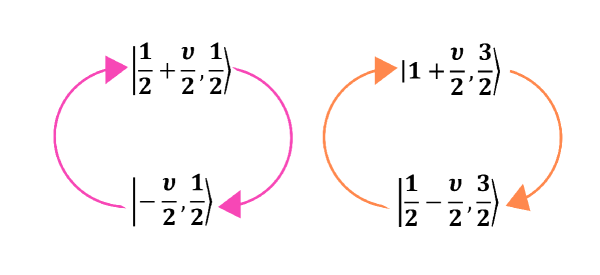
Figure 1: Loop of repeating states $\left|-\frac{\upsilon}{2},\frac{1}{2}\right\rangle\circlearrowleft\left|\frac{1}{2}+\frac{\upsilon}{2},\frac{1}{2}\right\rangle$ and $\left|\frac{1}{2}-\frac{\upsilon}{2},\frac{3}{2}\right\rangle\circlearrowleft\left|1+\frac{\upsilon}{2},\frac{3}{2}\right\rangle$.

The parameter $\upsilon$ depend on the energy of the cosmic states and the space-time topology Eq. (4.7). Whereas the parameter $z$ depends on the Hubble parameter. The two parameters ($\upsilon,z$) are complex numbers, but they have an importance in our study. These parameters possess the remarkable ability to generate comprehensive information about the cosmic states.

5 Constraining Lovelock inflation by observation

Let us now briefly address the physical properties of the Lovelock inflation [35]. We note that cosmic inflation is a theory that describes the early universe in which the universe underwent a period of extremely rapid expansion [56, 57, 58]. In Lovelock gravity, the theory of inflation is modified due to the presence of higher-dimensional terms Eq. (3.2). To make a possible generation of new solutions for inflation in Lovelock gravity with the rescaled Lovelock coupling $H$, we define the slow roll parameter $\epsilon_{\mathcal{H}}=-\frac{\mathcal{\dot{H}}}{\mathcal{H}^{2}}\approx-\frac{\dot{H}-\frac{\kappa}{a^{2}}}{H^{2}+\frac{\kappa}{a^{2}}}$. The $\epsilon_{H}$ parameter is approximately given by $\epsilon_{\mathcal{H}}\approx\epsilon_{H}=-\dot{H}/H^{2}\ll 1$. Leads to

$$\mathcal{\dot{H}}=-\epsilon_{H}H\mathcal{H}.$$ (5.1)

Next, we calculate the derivative of $\epsilon_{H}$ by using Eq. (5.1)$\ \dot{\epsilon}_{H}=\dot{H}\epsilon_{H}^{2}-\frac{\mathcal{\ddot{H}}}{H\mathcal{H}}$. Following [62], the slow-roll parameter is given by $\eta=\epsilon_{H}-\frac{\dot{\epsilon}_{H}}{2H\epsilon_{H}}$. In the conventional inflationary scenario, the $\epsilon_{H}$ grows as well $d\epsilon_{H}/dN=2\epsilon_{H}\left(\eta-\epsilon_{H}\right)$. In this case, the spectral index of perturbations is equal to $n_{s}=1-6\epsilon_{H}+2\eta$ [62, 4]. We can estimate the spectral index by the ratio: $n_{s}=1-4\epsilon_{H}-\frac{\dot{H}}{H}\epsilon_{H}+\frac{\mathcal{\ddot{H}}}{\mathcal{H}H^{2}\epsilon_{H}}.$ Define the first potential slow-roll parameter $\epsilon_{V}=\frac{1}{16\pi G_{N}}\left[\frac{V^{\prime}}{V}\right]^{2}.$ One obtains $\epsilon_{V}=\frac{1}{16\pi G_{N}}\frac{n^{2}}{\mathcal{H}^{2}}$ where $\dot{V}=\frac{\partial V}{\partial t}$ and $V^{\prime}=\frac{\partial V}{\partial\mathcal{H}}$. We thus introduce the tensor-to-scalar ratio

$$r=16\epsilon_{V}=\frac{n^{2}}{\pi G_{N}\mathcal{H}^{2}}.$$ (5.2)

The number of e-foldings counted backward from the end of inflation can be estimated as $N=\int_{\mathcal{H}}^{\mathcal{H}_{end}}\frac{H}{\mathcal{\dot{H}}}dH$ [4]. The number $N$ describes the amount of expansion that occurs during the inflationary period and is related to the ratio of the final and initial sizes of the universe. The field value $H_{f}$ at the end of inflation is determined by the condition $\epsilon_{H}=1$. Using $\dot{H}=\epsilon_{H}HH$. Then, the number of e-folds can be given by

$$N=\frac{1}{\epsilon_{H}}\int_{\mathcal{H}}^{\mathcal{H}_{end}}d\ln\mathcal{H}=\frac{1}{\epsilon_{H}}\ln\frac{\mathcal{H}_{end}}{\mathcal{H}}.$$ (5.3)

The effective energy density and pressure of the scalar field are modified, which can affect the dynamics of inflation and the value of the Hubble parameter during the inflationary period. This, in turn, can affect the value of $N$. On using Eq. (5.3), we can express the rescaled Lovelock coupling in the forms

$$\mathcal{H}=\mathcal{H}_{end}e^{-N\epsilon_{H}}.$$ (5.4)

From [64], the term $e^{-2N}=\left(\frac{\mathcal{H}}{\mathcal{H}_{end}}\right)^{\frac{2}{\epsilon_{H}}}$ describes the ratio between the initial and the final phase of inflation. The evolution of the rescaled Lovelock coupling is governed by $\frac{\mathcal{\dot{H}}}{\mathcal{H}}=-\left(\dot{N}\epsilon_{H}+N\dot{\epsilon}_{H}\right)$. It is worth noticing that $r=\frac{n^{2}}{\pi G_{N}\mathcal{H}_{end}^{2}}e^{2N\epsilon_{H}}$. The e-folds before the end of inflation for the formation of the visible part of the Universe is $N=60$ [59, 60, 61], i.e. $\dot{N}=0$. From this and Eq. (5.1) we find $N\dot{\epsilon}_{H}=H\epsilon_{H}$. Thus, we can find a useful relation between $\eta$ and $N$ as $\eta=\epsilon_{H}-\frac{1}{2N}$. The spectral index reduces to

$$n_{s}=1-4\epsilon_{H}-\frac{1}{N}.$$ (5.5)

This expression is in good agreement with that found in [57]. The Planck CMB data implies that $n_{s}\approx 0.965\pm 0.0042$ [63]. For simplicity, Eq. (5.4) can be approximately obtained as $1-\frac{\mathcal{H}}{\mathcal{H}_{end}}\approx N\epsilon_{H}$, or equivalently $\left(1-n_{s}\right)N=1+4\left(1-\frac{\mathcal{H}}{\mathcal{H}_{end}}\right)$. We find

$$n_{s}=1-\frac{5}{N}+\frac{4\mathcal{H}}{N\mathcal{H}_{end}}.$$ (5.6)

We first focus on $N=60$. In particular, for the case with $H=H_{end}$, we have $n_{s}\left(\mathcal{H}_{end}\right)=1-\frac{1}{N}\approx 0.983$, and for the case with $H=2H_{end}$, we have $n_{s}\left(2\mathcal{H}_{end}\right)\approx 1+\frac{3}{N}=1.05$. Additionally, for $H_{\min}=\frac{1}{2}H_{end}$ and $H_{\min}=\frac{3}{4}H_{end}$ we have $n_{s}=0.95$ and $n_{s}=0.96$, respectively. As a result, the observational constraint derived from the recent Planck 2018 data [63] already rules out the class of the inflation model when $\frac{1}{2}H_{end}<H<H_{end}$. From this condition we get $\frac{1}{2}<e^{-N\epsilon_{H}}<1$, which leads to $0<\epsilon_{H}<\frac{1}{2N}$.

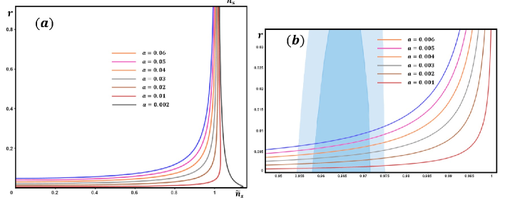
Figure 2: (a) The spectral index $\tilde{n}_{s}$ as a function of $r$ for $b=0.05$. (b) The curves correspond to the spectral index $\tilde{n}_{s}$ as a function of $r$ for $b=0.0005$. The Lovelock gravity framework yields predictions for the spectral tilt and tensor-to-scalar ratio within the context of inflation.

One can further define a new spectral index $\tilde{n}_{s}=n_{s}+\frac{5}{N}=n_{s}+0.083$, such that Eq. (5.6) can be expressed $\tilde{n}_{s}-\frac{4}{N\mathcal{H}_{end}}H=1.$ Let us comment on the spectral index in the monomial inflation. From Eqs. (5.2,5.6) we have $\tilde{n}_{s}^{2}+\frac{16}{N^{2}\mathcal{H}_{end}^{2}}H^{2}-\frac{8\tilde{n}_{s}\mathcal{H}}{N\mathcal{H}_{end}}=1,$or equivalently,

$$\tilde{n}_{s}^{2}+\frac{16n^{2}}{\pi G_{N}N^{2}\mathcal{H}_{end}^{2}}\frac{1}{r}-\frac{8\tilde{n}_{s}n}{N\mathcal{H}_{end}}\sqrt{\frac{1}{\pi G_{N}r}}=1.$$ (5.7)

From which one finds that $\tilde{n}_{s}^{2}+\frac{a}{r}-\frac{b}{\sqrt{r}}=1$, where $a=\frac{16n^{2}}{\pi G_{N}N^{2}\mathcal{H}_{end}^{2}}$ and $b=\frac{8\tilde{n}_{s}n}{N\mathcal{H}_{end}\sqrt{\pi G_{N}}}$. From which, we plot the predictions in the $\tilde{n}_{s}$ vs $r$ plane for the case $b=0.05$ see Fig. 2-(a) and $b=0.0005$ in Fig. 2-(b).

6 Conclusion

To summarize, this study examines the properties of cosmic acceleration within the Friedmann-Robertson-Walker metric, considering the density, potential, and equation of state in relation to the Hubble parameter and the Lovelock coupling. The energy states of cosmic acceleration are explored through the Lovelock densities and the Schrödinger equation. The rescaled Hubble parameter directly linked to cosmic acceleration by the energy density, is shown to be crucial for understanding the dynamics of the universe. Quantum states are found to follow a parabolic cylinder function, with hypergeometric functions acting as creation and annihilation operators. A family of symmetric numbers is proposed to generate the energy spectrum of cosmic acceleration. We have found that there is a possibility of looping the quantum states of cosmic acceleration. The analysis focuses on specific hypergeometric states in Lovelock gravity, revealing important insights into the kinetic energy and mass within the density parameters. Finally, the study discusses the diverse quantum properties associated with cosmic acceleration.
By exploring the predicted spectral tilt and tensor-to-scalar ratio, the study offers valuable insights into the observational consequences of the proposed models. The plotted curves effectively depict these predictions, providing a visual representation of the theoretical findings. An essential aspect of this work is the determination of the spectral index in terms of the number of e-folds, achieved through the utilization of the obtained inflaton field. The proposed concept of Lovelock couplings as representing a topological mass, which characterizes the Lovelock branch, introduces a novel perspective on the underlying physics and offers potential for further exploration, including a quantum description.
In summary, this research provides valuable insights into chaotic inflation within Lovelock gravity, with implications for our understanding of the early universe and its inflationary dynamics.
Acknowledgments
The authors thanks Andronikos Paliathanasis for useful enlightening discussions on the subject of cosmic acceleration and inflaton field. We thank Neda Farhangkhah and Liu Zhao for their detailed comments on the Lovelock gravity and dark energy.

7 Appendix A

From Eq. (4.2) we have

$$\frac{\partial^{2}\psi\left(H\right)}{\partial H^{2}}+\frac{2m}{H^{2}}\left(E-V\right)\psi\left(H\right)=0.$$ (7.1)

Using $m=\rho V$ we obtain

$$\frac{\partial^{2}\psi\left(H\right)}{\partial H^{2}}+\frac{2\rho\mathcal{V}}{H^{2}}\left(E-V\right)\psi\left(H\right)=0.$$ (7.2)

Substituting Eq. (3.2): $\rho=\sum_{n=1}^{\bar{D}}g_{n}^{2}H^{2n}$ in Eq. (7.2) we get

$$\frac{\partial^{2}\psi\left(H\right)}{\partial H^{2}}+\frac{2\mathcal{V}}{H^{2}}\left(E-V\right)\sum_{n=1}^{\bar{D}}g_{n}^{2}\mathcal{H}^{2n}\psi\left(H\right)=0,$$ (7.3)

or equivalently

$$\frac{\partial^{2}\psi\left(H\right)}{\partial H^{2}}+\frac{2\mathcal{V}}{H^{2}}\left(E-V\right)\sum_{n=1}^{\bar{D}}\left(g_{1}^{2}\mathcal{H}^{2}+\cdots+g_{\bar{D}}^{2}\mathcal{H}^{2\bar{D}}\right)\psi\left(H\right)=0.$$ (7.4)

On the other hand from Eq. (3.1): $H^{2}=H^{2}+\frac{\kappa}{a^{2}}$and Eq. (7.3) we obtain

$$\frac{\partial^{2}\psi\left(H\right)}{\partial H^{2}}+\frac{2\mathcal{V}}{H^{2}}\left(E-V\right)\sum_{n=1}^{\bar{D}}g_{n}^{2}\left(H^{2}+\frac{\kappa}{a^{2}}\right)^{n}\psi\left(H\right)=0.$$ (7.5)

In the regime of $V\ll E$, $\kappa=0$ and $D=4$ , i.e. $\bar{D}=2$, Eq. (7.5) can be written as

$$\frac{\partial^{2}\psi\left(H\right)}{\partial H^{2}}+2\mathcal{V}E\left(g_{1}^{2}+g_{2}^{2}H^{2}\right)\psi\left(H\right)=0.$$ (7.6)

The solution of Eq. (7.6) can be written as

$$\psi\left(H\right)=\psi_{0-}\mathcal{D}_{\bar{\upsilon}}\left(\left(1+i\right)HB\right)+\psi_{0+}\mathcal{D}_{\upsilon}\left(-\left(1-i\right)HB\right).$$ (7.7)

Here, $D$ is the parabolic cylinder function [52, 53], where

$$\upsilon = -\frac{1}{2}+\frac{ig_{1}^{2}}{2}\sqrt{\frac{2E\mathcal{V}}{g_{2}^{2}}},$$ (7.8)

$$\bar{\upsilon} = -\frac{1}{2}-\frac{ig_{1}^{2}}{2}\sqrt{\frac{2E\mathcal{V}}{g_{2}^{2}}},$$

$$B = \left(2E\mathcal{V}g_{2}^{2}\right)^{\frac{1}{4}}.$$

We recall that $\left|z\right|^{2}=z\bar{z}=\left(x+iy\right)\left(x-iy\right)=x^{2}+y^{2}$. From Eqs. (7.7) we have

$$\left|\upsilon\right|^{2}=\upsilon\bar{\upsilon}=\left(-\frac{1}{2}\right)^{2}+\frac{g_{1}^{4}}{4}\frac{2E\mathcal{V}}{g_{2}^{2}},$$ (7.9)

$$\frac{g_{1}^{4}}{4}\frac{2E\mathcal{V}}{g_{2}^{2}}=\left|\upsilon\right|^{2}-\frac{1}{4},$$ (7.10)

$$E=\frac{2g_{2}^{2}}{\mathcal{V}g_{1}^{4}}\left(\left|\upsilon\right|^{2}-\frac{1}{4}\right).$$ (7.11)

From Eqs. (2.6)-(3.1) we have $\frac{g_{2}^{2}}{g_{1}^{4}}=\frac{\alpha_{2}}{6}$. This leads to Eq. (4.7):

$$E=\frac{\alpha_{2}}{3\mathcal{V}}\left(\left|\upsilon\right|^{2}-\frac{1}{4}\right).$$ (7.12)

References

- [1] D. Lovelock, J. Math. Phys., 12(3), 498-501 (1971).
- [2] P. Bueno, P. A. Cano and P. F. Ramírez, JHEP, 2016(4), 1-40 (2016).
- [3] N. C. Bai, L. Li, J. Tao, Phys. Rev. D, 107(6), 064015 (2023).
- [4] G. Alkaç, G. Süer, Phys. Rev. D, 107(4), 046014 (2023).
- [5] E. Babichev, C. Charmousis, M. Hassaine, N. Lecoeur, Phys. Rev. D, 107(8), 084050 (2023).
- [6] X. Q. Li, B. Chen and L. L. Xing, Ann. Phys., 446, 169125 (2022).
- [7] A. Ali and K. Saifullah, Eur. Phys. J. C, 82(5), 408 (2022).
- [8] A. Ali, and K. Saifullah, Phys. Rev. D, 99(12), 124052 (2019).
- [9] B. P. Brassel, R. Goswami and S. D. Maharaj, Ann. Phys., 446, 169138 (2022).
- [10] A. Ali and K. Saifullah, Ann. Phys., 446, 169094 (2022).
- [11] Z. Amirabi, Ann. Phys., 443, 168990 (2022).
- [12] M. Estrada, Ann. Phys., 439, 168792 (2022).
- [13] M. H. Dehghani and N. Farhangkhah, Physical Review D, 78(6), 064015 (2008).
- [14] N. Farhangkhah, Phys. Rev. D, 97(8), 084031 (2018).
- [15] N. Farhangkhah and Z. Dayyani, Phys. Rev. D, 104(2), 024068 (2021).
- [16] T. Padmanabhan and D. Kothawala, Phys. Rep., 531(3), 115-171 (2013).
- [17] A. Paranjape, S. Sarkar and T. Padmanabhan, Phys. Rev. D, 74(10), 104015 (2006).
- [18] A. Mardones and J. Zanelli, Class. Quant. Grav., 8(8), 1545 (1991).
- [19] X. O. Camanho and J. D. Edelstein, JHEP, 2010(6), 1-35 (2010).
- [20] G. Papallo and H. S. Reall, Phys. Rev. D, 96(4), 044019 (2017).
- [21] N. Deruelle and L. Farina-Busto, Phys. Rev. D, 41(12), 3696 (1990).
- [22] X. H. Meng and P. Wang, Class. Quantum Gravity, 20(22), 4949 (2003).
- [23] M. Bousder, E. Salmani, A. El Fatimy, H. Ez-Zahraouy, Ann. Phys., 452, 169282 (2023).
- [24] R. G. Cai and S. P. Kim, JHEP, 2005(02), 050 (2005).
- [25] R. G. Cai, L. M. Cao and Y. P. Hu, JHEP, 2008(08), 090 (2008).
- [26] T. Demaerel, C. Maes and W. Struyve, Class. Quantum Gravity, 37(8), 085006, (2020).
- [27] B. P.Dolan, A. Kostouki, D. Kubizňák and R. B. Mann, Class. Quant. Grav., 31(24), 242001 (2014).
- [28] A. F. Ali and S. Das, Phys. Lett. B, 741, 276-279 (2015).
- [29] S. Capozziello, A. Feoli and G. Lambiase, Int. J. Mod. Phys. D, 9(02), 143-154, (2000).
- [30] R. Johnston, A. N. Lasenby and M. P. Hobson, MNRAS, 402(4), 2491-2502 (2010).
- [31] J. Martin, V. Vennin and P. Peter, Phys. Rev. D, 86(10), 103524 (2012).
- [32] N. Rosen, Int. J. Theor. Phys., 32, 1435-1440 (1993).
- [33] B. S. DeWitt, Phys. Rev., 160(5), 1113 (1967).
- [34] H. Everett III, Rev. Mod. Phys., 29(3), 454 (1957).
- [35] F. Ferrer and S. Räsänen, J. High Energy Phys., 2007(11), 003 (2007).
- [36] M. Bousder, Journal of Cosmology and Astroparticle Physics, 2022(01), 015 (2022).
- [37] M. Bousder and M. Bennai, Phys. Lett. B, 817, 136343 (2021).
- [38] D. Kastor, S. Ray, J. Traschen, Class. Quant. Grav., 34(19), 195005 (2017).
- [39] R. G. Cai, L. M. Cao, Y. P. Hu and S. P. Kim, Phys. Rev. D, 78(12), 124012 (2008).
- [40] P. G. Fernandes, P. Carrilho, T. Clifton, D. J. Mulryne, Class. Quant. Grav., 39(6), 063001 (2022).
- [41] R. G. Cai, Phys. Lett. B, 582(3-4), 237-242 (2004).
- [42] T. L. Smith, V. Poulin and M. A. Amin. Phys. Rev. D, 101(6), 063523, (2020).
- [43] S. Capozziello, Int. J. Mod. Phys. D, 11(04), 483-491 (2002).
- [44] S. Capozziello, S. Carloni, A. Troisi, arXiv preprint astro-ph/0303041 (2003).
- [45] L. Verde, T. Treu and A. G. Riess, Nat. Astron, 3(10), 891-895 (2019).
- [46] M. Kawasaki, M. Yamaguchi and T. Yanagida, Phys. Rev. Lett., 85(17), 3572 (2000).
- [47] M. M. Caldarelli, G. Cognola, and D. Klemm, Class. Quant. Grav., 17(2), 399 (2000).
- [48] R. Nasri, Integral Transforms Spec. Funct., 27(3), 181-196 (2016).
- [49] N. M. Temme, J. Comput. Appl. Math., 121(1-2), 221-246 (2000).
- [50] D. Veestraeten, Integral Transforms Spec. Funct., 28(1), 15-21 (2017).
- [51] Á. Baricz and M. E. Ismail, Constr. Approx., 37, 195-221 (2013).
- [52] N. M. Temme, J. Comput. Appl. Math., 121(1-2), 221-246 (2000).
- [53] M. R. K. Vahdani, G. Rezaei, Phys. Lett. A, 374(4), 637-643 (2010).
- [54] M. Bousder, E. Salmani, H. Ez-Zahraouy, J. High Energy Phys., 38, 49-57, 2023 (2023).
- [55] K. Giesel, D. Winnekens, Class. Quant. Grav., 40(8), 085013 (2023)..
- [56] S. C. Hyun, J. Kim, S. C. Park, T. Takahashi, J. Cosmol. Astropart. Phys., 2022(05), 045 (2022).
- [57] Y. Morishita, T. Takahashi, S. Yokoyama, J. Cosmol. Astropart. Phys., 2022(07), 042 (2022).
- [58] M. Kubota, K. Y. Oda, S. Rusak, T. Takahashi. J. Cosmol. Astropart. Phys., 2022(06), 01, (2022).
- [59] S. Clesse, B. Garbrecht and Y. Zhu, Phys. Rev. D, 89(6), 063519 (2014).
- [60] A.Linde and A. Riotto, Phys. Rev. D, 56(4), R1841 (1997).
- [61] K. Dimopoulos, Phys. Lett. B, 735, 75-78 (2014).
- [62] R. Maartens, D. Wands, B. A. Bassett and I. P. C. Heard, Phys. Rev. D, 62(4), 041301(R) (2000).
- [63] N. Aghanim, et al. Astron. Astrophys. (641) A6 (2020).
- [64] R. D’Agostino, O. Luongo and M. Muccino, Class. Quant. Grav., 39(19), 195014 (2022).
- [65] C. P. Herzog and K. W. Huang, Phys. Rev. D, 87(8), 081901 (2013).