NIPG-DG schemes for transformed master equations modeling open quantum systems

Abstract

This work presents a numerical analysis of a master equation modeling the interaction of a system with a noisy environment in the particular context of open quantum systems. It is shown that our transformed master equation has a reduced computational cost in comparison to a Wigner-Fokker-Planck model of the same system for the general case of any potential. Specifics of a NIPG-DG numerical scheme adequate for the convection-diffusion system obtained are then presented. This will let us solve computationally the transformed system of interest modeling our open quantum system. A benchmark problem, the case of a harmonic potential, is then presented, for which the numerical results are compared against the analytical steady-state solution of this problem.

1 Introduction

Open quantum systems model the interaction (energy exchange, for example) of a system with a usually larger environment in a quantum setting. They are mathematically expressed in quantum information science by master equations in Lindblad form (when a Markovian dynamics in the interaction is assumed) for the density matrix of the system [20] (to describe, for example, a noisy quantum channel). These Lindblad master equations can be converted into Wigner-Fokker-Planck (WFP) equations by applying to them a Wigner transform [6, 3]. The density matrix is converted under this transformation into the Wigner function representing the system. The Wigner-Fokker-Planck formulation is then, mathematically, completely equivalent to the Lindblad master equation description of open quantum systems. The quantum Fokker-Planck operator terms (which are the analogs in the Wigner formulation of the Lindblad operators of the master equation) represent the diffusive behavior of the system plus a friction term, both due to the interaction with the environment, via energy exchanges, for example, as abovementioned.

The following dimensionless model of an open quantum system will be first considered, which is given by the WFP equation with an arbitrary potential as below [3, 8]

$$w_{t}+k\cdot\nabla_{x}w+\Theta[V]{w}=Q_{FP}\{w\},$$

where $Q_{FP}$ is the quantum Fokker-Planck operator that models the interaction of the system with its environment (representing it in the Wigner picture by a diffusion term plus a friction one, as abovementioned). The following particular case for the aforementioned operator will be considered,

$$Q_{FP}\{w\}=\Delta_{k}w+\nabla_{k}\cdot(kw)+\Delta_{x}w,$$

and the pseudo-differential operator (non-local) related to the potential $V$ is given by

$$\Theta[V]\{w\}=\frac{-i}{(2\pi)^{d}}\int_{\mathcal{\mathcal{R}}^{2d}}\delta V(x,\eta)w(x,k^{\prime},t)e^{i\eta\cdot(k-k^{\prime})}dk^{\prime}d\eta,$$

$$\delta V(x,\eta)=V(x+\eta/2)-V(x-\eta/2),$$

which can also be represented as

$$\Theta[V]\{w\}=\frac{-i}{(2\pi)^{d}}\int_{\mathcal{\mathcal{R}}^{d}}[V(x+\eta/2)-V(x-\eta/2)]\mathcal{F}\{w\}e^{i\eta\cdot k}d\eta,$$

with $\mathcal{F}\{w\}$ the Fourier transform of our Wigner function $w$,

$$\mathcal{F}\{w\}(x,\eta,t)=\int_{\mathcal{\mathcal{R}}^{d}}w(x,k^{\prime},t)e^{-i\eta\cdot k^{\prime}}dk^{\prime}.$$

The pseudo-differential operator is the computationally costliest term in a simulation of the WFP system, due to the extra integration needed to be performed in order to compute it [8]. However, it is clear that, if a Fourier transform is applied to it, it will amount just to a multiplication by convolution theorems. Therefore, this motivates the interest in applying a Fourier transform to the Wigner function to simply obtain a density matrix in the position basis, with conveniently transformed coordinates. If a Fourier transform is then applied to the WFP system, a master equation will simply be obtained in convenient coordinates that simplifies the expression of the costliest term, namely the one related to the potential. A similar evolution equation for a density in transformed coordinates has been presented in [12] in the context of electron ensembles in semiconductors. The above-mentioned is justified by recalling that the Wigner function is defined by the Fourier transform below,

$$w(x,k,t)=\int_{\mathcal{R}^{d}}\rho(x+\eta/2,x-\eta/2,t)\exp(-i\eta\cdot k)d\eta,$$ (1)

particularly as the Fourier transform of the function

$$u(x,\eta,t)=\rho(x+\eta/2,x-\eta/2,t),$$ (2)

which is a density matrix in terms of conveniently symmetrized position coordinates. Therefore,

$$w=\mathcal{F}\{u\},\quad u=\mathcal{F}^{-1}\{w\},$$ (3)

and then

$$u(x,\eta,t)=\frac{1}{(2\pi)^{d}}\int_{\mathcal{R}^{d}}w(x,k,t)\exp(ik\cdot\eta)dk=$$ (4)

$$=\frac{1}{(2\pi)^{d}}\int_{\mathcal{R}^{d}}w(x,k,t)e^{-ik\cdot[-\eta]}dk=\frac{\mathcal{F}\{w\}(x,-\eta,t)}{(2\pi)^{d}}.$$ (5)

So our Fourier transform is just proportional to the density matrix evaluated at conveniently transformed position coordinates,

$${\mathcal{F}\{w\}(x,\eta,t)}={(2\pi)^{d}}\rho(x-\eta/2,x+\eta/2,t).$$ (6)

Different numerical methods have been used in the computational simulation of models for open quantum systems. Regarding computational modeling of open quantum systems via Wigner functions, stochastic methods such as Monte Carlo simulations of Fokker-Planck equations in Quantum Optics have been reported [5], as well as numerical discretizations of velocities for the stationary Wigner equation[7]. However, there is an inherent stochastic error in the solution of PDE’s by Monte Carlo methods (where this error will decrease slowly, as $N^{-1/2}$, by increasing the number of samples $N$). There is literature on the Wigner numerical simulation of quantum tunneling phenomena [21], as well as work on operator splitting methods for Wigner-Poisson [4], and on the semidiscrete analysis of the Wigner equation [10]. However, the nature of the phenomena for open quantum systems claims the need for a numerical method that reflects in its nature the physics of both transport and noise represented by diffusion (for Markovian interactions), therefore the interest on Discontinuous Galerkin (DG) methods that can mimic numerically convection-diffusion problems, such as Local DG or Interior Penalty methods, for example. There is work in [8] on an adaptable DG scheme for Wigner-Fokker-Planck, where a Non-symmetric Interior Penalty Galerkin method is used for the computational modeling. The main issue of the use of a Wigner model for open quantum systems though is the fact that, except for the case of harmonic potentials, the costliest term computationally in a Wigner formulation is the pseudo-differential integral operator, whereas a simple Fourier transformation of the Wigner equation might render this term as just a simple multiplication between the related density matrix and the (non-harmonic) potential and therefore not computationally costly anymore in a master equation setting. There are literature reports of the appliciation of Discontinuous Galerkin Methods onto Quantum-Liouville type equations [9], and numerical simulations of the Quantum Liouville-Poisson system as well [26]. However this kind of equations consider only the quantum transport part of the problem, since diffusion does not appears in Liouville transport, so noise due to an environment is missing to be modeled in a DG setting for master equations up to the author’s knowledge.

The contribution of the work presented in this paper then is to provide a computational solver for open quantum systems, modeled by transformed master equations, whose underlying numerics reflects inherently in its methodology the convection-diffusion nature of the physical phenomena of interest, solving the resulting system of master equations by means of a Non-symmetric Interior Penalty Discontinuous Galerkin method to handle both the quantum transport and the diffusive noise due to environment interactions, at a less expensive computational cost than a Wigner model for the open quantum problem of interest.

The summary of our work is the following: convolution theorems of Fourier transforms will be used to convert our pseudo-differential operator into a product, transforming then the WFP into a master equation for the density matrix in symmetrized position coordinates. The remaining terms (transport and diffusion) will be analyzed, and the transformed master equation will be studied numerically via an NIPG-DG method, as an initial/boundary value problem (IBVP) in a 2D position space, reducing the computational cost of the time evolution problem over its process with respect to WFP conveniently via our transformed master equation formulation. Finally, convergence studies are presented for a problem with a harmonic potential, for which the analytical steady-state solution is known (the harmonic oscillator case), comparing it to the numerical solution obtained via the NIPG-DG method.

2 Math Model: Transformed Master Equation for open quantum systems

It is known that the pseudo-differential operator has the following possible representation,

$$\Theta[V]\{w\}=-w\star\Im(F^{-1}[\delta V]),$$

$$F^{-1}\{F\{w\}\cdot F\{\Im(F^{-1}[\delta V])\}\}=w\star\Im(F^{-1}[\delta V])=-\Theta[V],$$

which simplifies to

$$\Theta[V]\{w\}=-F^{-1}\{\widehat{w}\cdot\frac{\delta V-F\{(F^{-1}[\delta V])^{*}\}}{2i}\}.$$

Since it holds that

$$F\{(F^{-1}[\delta V])^{*}\}=F\{\frac{\int_{\mathcal{\mathcal{R}}^{d}}[V(x+\frac{\eta^{\prime}}{2})-V(x-\frac{\eta^{\prime}}{2})]e^{-ik\cdot\eta^{\prime}}d\eta^{\prime}}{(2\pi)^{d}}\},$$

$$F\{\frac{\int_{\mathcal{\mathcal{R}}^{d}}[V(x-\frac{\eta^{\prime}}{2})-V(x+\frac{\eta^{\prime}}{2})]e^{ik\cdot\eta^{\prime}}d\eta^{\prime}}{(2\pi)^{d}}\}=-\delta V(x,\eta),$$

then

$$w_{t}+k\cdot\nabla_{x}w+iF^{-1}\{\widehat{w}\cdot{\delta V}\}=\Delta_{k}w+\nabla_{k}\cdot(kw)+\Delta_{x}w,$$

and applying a Fourier transform to WFP, it acquires the form

$$\widehat{w}_{t}+\widehat{k\cdot\nabla_{x}w}+i\widehat{w}\cdot{\delta V}=\widehat{\Delta_{k}w}+\widehat{\nabla_{k}\cdot(kw)}+\Delta_{x}\widehat{w}.$$

The forward Fourier transform of the WFP equation is then the transformed master equation below,

$$\widehat{w}_{t}+i\nabla_{\eta}\cdot\nabla_{x}\widehat{w}+i\widehat{w}\cdot{\delta V}=-\eta^{2}\widehat{w}-\eta\cdot\nabla_{\eta}\widehat{w}+\Delta_{x}\widehat{w}.$$ (7)

It is clear that the pseudo-differential operator over the potential represented by a convolution has been transformed back into a product of functions by Fourier transforming the WFP equation. The main change is that the transport term is represented now as a derivative of higher order ($k$ was exchanged for $i\nabla_{\eta}$ when transforming into the Fourier space).

2.1 Decomposition into real and imaginary parts

If one starts with

$$\widehat{w}_{t}+\nabla_{x}\cdot(i\nabla_{\eta}\widehat{w})+\eta\cdot\nabla_{\eta}\widehat{w}=\widehat{w}\cdot\left(\frac{\delta V}{i}-\eta^{2}\right)+\nabla_{x}^{2}\widehat{w},$$

it can be noticed that the transport term involves a complex number, so $\widehat{w}=R+iI$ will be decomposed into real and imaginary parts to rather better understand this term. So

$$[R+iI]_{t}+\nabla_{x}\cdot(i\nabla_{\eta}[R+iI])+\eta\cdot\nabla_{\eta}[R+iI]=$$

$$[R+iI]\cdot\left(\frac{\delta V}{i}-\eta^{2}\right)+\nabla_{x}^{2}[R+iI],$$

then

$$R_{t}+iI_{t}+\nabla_{x}\cdot\nabla_{\eta}[-I+iR]+\eta\cdot\nabla_{\eta}[R+iI]=$$

$$[R+iI]\cdot\left(\frac{\delta V}{i}\right)-[R+iI]\cdot\left(\eta^{2}\right)+\nabla_{x}^{2}[R+iI].$$

Let’s focus now on the benchmark case of dimension $d=1,$ for which many terms simplify. In this case

$$R_{t}+iI_{t}+\partial_{x}\partial_{\eta}[-I+iR]+\eta\partial_{\eta}[R+iI]=$$

$$[R+iI]\cdot\left(\frac{\delta V}{i}\right)-[R+iI]\eta^{2}+\nabla_{x}^{2}[R+iI].$$

Then

$$R_{t}+iI_{t}+\partial_{x\eta}[-I+iR]+\eta\partial_{\eta}[R+iI]=[I-iR]\cdot\left(\frac{\delta V}{2}\right)$$

$$+[-I+iR]\cdot\left(\frac{\delta V}{2}\right)-[R+iI]\eta^{2}+\nabla_{x}^{2}[R+iI],$$

so

$$R_{t}+iI_{t}+\partial_{x\eta}[-I+iR]+\eta\partial_{\eta}[R+iI]=[I-iR]\cdot\left({\delta V}\right)$$

$$-[R+iI]\eta^{2}+\nabla_{x}^{2}[R+iI],$$

and now the equation can be decomposed into real and imaginary parts. The real part of the equation is

$$R_{t}-\partial_{x\eta}I+\eta\partial_{\eta}R=I{\delta V}-R\eta^{2}+\nabla_{x}^{2}R,$$

and the imaginary part is

$$I_{t}+\partial_{x\eta}R+\eta\partial_{\eta}I=-R\cdot\left({\delta V}\right)-I\eta^{2}+\nabla_{x}^{2}I,$$

where, since $d=1,$ the Laplacian reduces to $\partial_{x}^{2}$, so we have the following system

$$R_{t}+\eta\partial_{\eta}R=I\left({\delta V}\right)-R\eta^{2}+\partial_{x}^{2}R+\partial_{x\eta}I,$$

$$I_{t}+\eta\partial_{\eta}I=-R\cdot\left({\delta V}\right)-I\eta^{2}+\partial_{x}^{2}I-\partial_{x\eta}R.$$

The system above has the transport terms on the left-hand side. The “source”, decay, and diffusive terms represented by second-order partials are on the right-hand side. If the transport is to be expressed in divergence form, one can pass the extra term to the other side, rendering

$$R_{t}+\partial_{\eta}(\eta R)=I\left({\delta V}\right)+(1-\eta^{2})R+\partial_{x}^{2}R+\partial_{x\eta}I,$$

$$I_{t}+\partial_{\eta}(\eta I)=-R\cdot\left({\delta V}\right)+(1-\eta^{2})I+\partial_{x}^{2}I-\partial_{x\eta}R.$$

These convective-diffusive systems (where the transport is only on $\eta$) can be expressed in matrix form. The matrix system in gradient form is

$$\partial_{t}\left(\begin{array}[]{c}R\\ I\end{array}\right)+\eta\partial_{\eta}\left(\begin{array}[]{c}R\\ I\end{array}\right)=-\left(\begin{array}[]{cc}\eta^{2}&-{\delta V}\\ {\delta V}&\eta^{2}\end{array}\right)\left(\begin{array}[]{c}R\\ I\end{array}\right)$$

$$+\left(\begin{array}[]{cc}\partial_{x}&\partial_{\eta}\\ -\partial_{\eta}&\partial_{x}\end{array}\right)\left(\begin{array}[]{c}\partial_{x}R\\ \partial_{x}I\end{array}\right),$$

or in divergence form as

$$\partial_{t}\left(\begin{array}[]{c}R\\ I\end{array}\right)+\partial_{\eta}\{\left(\begin{array}[]{c}R\\ I\end{array}\right)\otimes(0,\eta)\}=$$

$$-\left(\begin{array}[]{cc}\eta^{2}-1&{-\delta V}\\ {\delta V}&\eta^{2}-1\end{array}\right)\left(\begin{array}[]{c}R\\ I\end{array}\right)+\left(\begin{array}[]{cc}\partial_{x}&\partial_{\eta}\\ -\partial_{\eta}&\partial_{x}\end{array}\right)\left(\begin{array}[]{c}\partial_{x}R\\ \partial_{x}I\end{array}\right).$$

In both of them, it is evident the left-hand side has a convective transport structure and the right-hand side has matrix terms related to decay, source (partly due to the potential), and diffusive behavior. If we define $u=(R,I)^{T}$ we can express the system in gradient form as

$$\partial_{t}u+\partial_{(x,\eta)}u\cdot\left(\begin{array}[]{c}0\\ \eta\end{array}\right)=\left(\begin{array}[]{cc}\partial_{x}&\partial_{\eta}\\ -\partial_{\eta}&\partial_{x}\end{array}\right)\partial_{x}u-\left(\begin{array}[]{cc}\eta^{2}&-{\delta V}\\ {\delta V}&\eta^{2}\end{array}\right)u,$$

or equivalently in divergence form as

$$\partial_{t}u+\partial_{(x,\eta)}\cdot\{u\otimes(0,\eta)\}=-\left(\begin{array}[]{cc}\eta^{2}-1&{-\delta V}\\ {\delta V}&\eta^{2}-1\end{array}\right)u$$

$$+\partial_{(x,\eta)}\cdot\left(\partial_{x}u,J\partial_{x}u\right),$$

defining the matrix

$$J=\left(\begin{array}[]{cc}0&1\\ -1&0\end{array}\right).$$

So the transport is only vertical, and the gradient in the diffusion term is only related to $x$-partials.

3 Methodology: DG Formulation for Master Equations in transformed position coordinates

A NIPG-DG scheme for a vector variable will be presented for our master equation (where the test function will be a vector too), and where we will perform an inner product multiplication between these vector functions to obtain the weak form for our related NIPG-DG methodology.

3.1 NIPG-DG method for a transformed Master Equation

Below one proceeds to describe then how to solve the system resulting from a transformed master equation, in convenient position coordinates, by means of a Non-symmetric Interior-Penalty Galerkin (NIPG) DG method, as in [22, 8] for elliptic equations and Wigner-Fokker-Planck equations,respectively. In this type of DG method, some penalty terms are introduced in order to account for the diffusion when treated by DG methodologies. More information can be found in the references mentioned above.

The NIPG-DG formulation (at the semi-discrete level) for the transformed master equation system is then the following: Find $u=\left(R,I\right)^{T}$ such that, for all test functions $v=\left(w,z\right)^{T}$ the following holds,

$$\partial_{t}(v,u)=a(v,u),$$ (8)

with the bilinear form (which also includes the penalty terms) given by

$$a(u,v) = (\nabla w,A\nabla R-bR)+(\nabla z,A\nabla I-bI)+(\nabla w,B\nabla I)-(z,B\nabla R)$$

$$+(w,I\delta V)+(w,R\eta^{2})+(z,R\delta V)+(z,I\eta^{2})$$

$$+(\alpha/h)\langle[wn],A[Rn]\rangle+(\alpha/h)\langle[wn],B[In]\rangle+(\alpha/h)\langle[wn],A[Rn]\rangle$$

$$-\langle[wn],A\{\nabla R\}\rangle-\langle[wn],B\{\nabla R\}\rangle$$

$$-\langle\{\nabla w\},A[Rn]\rangle-\langle\{\nabla w\},B[In]\rangle$$

$$+(\alpha/h)\langle[zn],A[In]\rangle-(\alpha/h)\langle[zn],B[Rn]\rangle-\langle[zn],A\{\nabla I\}\rangle$$

$$+\langle[zn],B\{\nabla R\}\rangle-\langle\{\nabla z\},A[In]\rangle+\langle\{\nabla z\},B[Rn]\rangle$$

$$+\langle[w],[\widehat{b}R]\rangle+\langle w,\widehat{b}R\rangle++\langle[z],[\widehat{b}I]\rangle+\langle z,\widehat{b}I\rangle,$$

where $[\cdot]$ stands for jumps, $\{\cdot\}$ stands for averages, $(\cdot,\cdot)$ stands for volume integrals, $\langle\cdot,\cdot\rangle$ stands for surface integrals, $n$ stands for outward unit normals, $b=(0,\eta)^{T}$ stands for the transport vector in our 2D position domain, and $\widehat{b}=(b\cdot n+|b\cdot n|)/2$ is related to the upwind flux rule.

We discretize the time evolution by applying an implicit theta method. In order to advance from $u_{0}$ to $u$ in the next time-step, the method below is then used,

$$(v,u-u_{0})/\Delta t=\theta a(v,u)+(1-\theta)a(v,u_{0}),$$ (10)

where a value of $\theta=1/2\in[0,1]$ is chosen, since it is known that this value, among all possible in [0,1], gives the highest order of convergence for implicit time evolution methods [11].

4 Computational Cost of Master Equations vs WFP via NIPG-DG methods

Our particular case of the WFP equation has the form

$$w_{t}+k\cdot\nabla_{x}w-$$

$$\frac{i}{(2\pi)^{d}}\int_{\mathcal{\mathcal{R}}^{2d}}[V(x+\frac{\eta}{2})-V(x-\frac{\eta}{2})]w(x,k^{\prime},t)e^{i\eta\cdot(k-k^{\prime})}dk^{\prime}d\eta$$

$$=\nabla_{k}\cdot(kw)+\Delta_{x}w+\Delta_{k}w.$$

If the size of the global basis for $w(x,k,t)=\sum_{i=1}^{n}\sum_{j=1}^{m}\sum_{p=0}^{P}\chi_{ij}(x,k)c_{p}^{ij}(t)\phi_{p}^{ij}(x,k)$ is $N=(P+1)nm$, where $P+1$ is the dimension of our local polynomial basis, $n$ the number of intervals in $x$, $m$ the number of intervals in $k$, the dimension of the test space $\mathrm{span}\{v_{k}(x,k)\}_{k=1}^{N}=\mathrm{span}\{\{\{v_{p}^{ij}(x,k)\}_{p=0}^{P}\}_{i=1}^{n}\}_{j=1}^{m}$ will be the same, and an NIPG-DG formulation for the Wigner-Fokker-Planck equation would look like ( $1\leq q\leq N$ )

$$\sum_{i=1}^{n}\sum_{j=1}^{m}\sum_{p=0}^{P}(v_{q}^{ij}|\phi_{p}^{ij})\frac{dc_{p}^{ij}}{dt}\chi_{ij}-\sum_{i=1}^{n}\sum_{j=1}^{m}\sum_{p=0}^{P}(\nabla_{x}v_{q}^{ij}|k\phi_{p}^{ij})c_{p}^{ij}\chi_{ij}-\sum_{i=1}^{n}\sum_{j=1}^{m}\sum_{p=0}^{P}(\nabla_{k}v_{q}^{ij}\cdot k|\phi_{p}^{ij})c_{p}^{ij}\chi_{ij}$$

$$+\sum_{i=1}^{n}\sum_{j=1}^{m}\sum_{p=0}^{P}\left\langle[v_{q}^{ij}]|[k\phi_{p}^{ij}]\right\rangle c_{p}^{ij}\chi_{ij}+\sum_{i=1}^{n}\sum_{j=1}^{m}\sum_{p=0}^{P}\left\langle v_{q}^{ij}|k\phi_{p}^{ij}\right\rangle c_{p}^{ij}\chi_{ij}$$

$$+(v_{q}^{ij}|\int_{\mathcal{\mathcal{R}}^{2d}}\delta V(x,\eta)\phi(x,k^{\prime})\frac{e^{i\eta\cdot(k-k^{\prime})}}{i(2\pi)^{d}}dk^{\prime}d\eta)c_{p}^{ij}+$$

$$=-\sum_{i=1}^{n}\sum_{j=1}^{m}\sum_{p=0}^{P}(\nabla_{x}v_{q}^{ij}|\nabla_{x}\phi_{p}^{ij}c_{p}^{ij})\chi_{ij}-\sum_{i=1}^{n}\sum_{j=1}^{m}\sum_{p=0}^{P}(\nabla_{k}v_{q}^{ij}|\nabla_{k}\phi_{p}^{ij})c_{p}^{ij}\chi_{ij}+$$

$$+\sum_{i=1}^{n}\sum_{j=1}^{m}\sum_{p=0}^{P}(\alpha/h)\langle[v_{q}^{ij}n]|[c_{p}^{ij}\phi_{p}^{ij}n]\rangle-\sum_{i=1}^{n}\sum_{j=1}^{m}\sum_{p=0}^{P}\langle[v_{q}^{ij}n]|\{\nabla\phi_{p}^{ij}c_{p}^{ij}\}\rangle-\sum_{i=1}^{n}\sum_{j=1}^{m}\sum_{p=0}^{P}\langle\{\nabla v_{q}^{ij}\}|[\phi_{p}^{ij}a_{p}^{ij}n]\rangle$$

so we have, at the semi-discrete level, $11N$ operations related to matrix-vector multiplications, but we must consider the cost of computing the matrix elements. If we go into the details of the cost of each term, assuming we use a piece-wise polynomial basis as traditionally used in DG (nonzero only inside a given element) we will see that computing all terms but the pseudo-differential operator takes work of $O(10nm[P+1]^{2})$ integrations (due to the piece-wise nature of the spaces). Specifically, without considering the pseudo-differential term, we need $5nm[P+1]^{2}$ volume integrations and $5nm[P+1]^{2}$ surface integrals The pseudo-differential operator involves an integral over the phase space where the potential and the real and imaginary parts of the complex exponential are involved,

$$\sum_{r=1}^{n}\sum_{s=1}^{m}\sum_{p=0}^{P}(v_{q}^{ij}(x,k)|\int_{\eta_{r-}}^{\eta_{r+}}\int_{k_{s-}}^{k_{s+}}\delta V\phi_{p}^{rs}(x,k^{\prime})\frac{e^{i\eta\cdot(k-k^{\prime})}}{i(2\pi)^{d}}dk^{\prime}d\eta)c_{p}^{rs}\chi_{rs},$$

due to the non-local nature of the double integrals, so there are possible extra overlaps in comparison to the other terms. Due to the nature of the basis, namely, piece-wise functions constituted by polynomials multiplied by characteristic functions, the overlap in $x$ must happen in order to get nonzero terms, so only $i=r$ will contribute, but the overlap in $k$ will happen as a must in any case since the integration is over all momentum regions. Our integral reduces to

$$\sum_{r=1}^{n}\sum_{s=1}^{m}\sum_{p=0}^{P}(v_{q}^{ij}\chi^{ij}|\int_{\eta_{r-}}^{\eta_{r+}}\int_{k_{s-}}^{k_{s+}}\delta V\phi_{p}^{rs}(x,k^{\prime})\frac{e^{i\eta\cdot(k-k^{\prime})}}{i(2\pi)^{d}}dk^{\prime}d\eta)c_{p}^{rs}\chi_{rs}$$

$$=\sum_{s=1}^{m}\sum_{p=0}^{P}(v_{q}^{ij}\chi^{j}(k)|\int_{\eta_{i-}}^{\eta_{i+}}\int_{k_{s-}}^{k_{s+}}\delta V\phi_{p}^{is}(x,k^{\prime})\frac{e^{i\eta\cdot(k-k^{\prime})}}{i(2\pi)^{d}}dk^{\prime}d\eta)c_{p}^{rs}\chi_{rs},$$

so the computational cost of this term is in principle

$$nm^{2}[P+1]^{2}=N^{2}/m,$$

which is $m$ times the usual cost of the other terms. This proves that the pseudo-differential term is the computationally costliest in the WFP numerics.

On the other hand, the computational cost of our transformed master equation in convenient coordinates can be analyzed by considering

$$u=(R,I)=\sum_{i=1}^{n}\sum_{j=1}^{m}\sum_{p=0}^{P}\chi_{ij}(a_{p}^{ij}(t)\phi_{p}^{ij},d_{p}^{ij}(t)\phi_{p}^{ij})$$

and

$$v_{q}^{ij}=(w_{q}^{ij},z_{q}^{ij})$$

with equivalent trial/test spaces (respectively)

$$\mathrm{span}\{\phi_{p}^{ij}\}_{i=1,j=1,p=0}^{i\leq n,j\leq m,p\leq P},$$

$$\mathrm{span}\{v_{p}^{ij}\}_{i=1,j=1,p=0}^{i\leq n,j\leq m,p\leq P}$$

for this system formulation. We have then that the NIPG-DG weak form can be expressed as

$$\sum_{i=1}^{n}\sum_{j=1}^{m}\sum_{p=0}^{P}(v_{q}^{ij}|\phi_{p}^{ij})\frac{da_{p}^{ij}}{dt}\chi_{ij}+\sum_{i=1}^{n}\sum_{j=1}^{m}\sum_{p=0}^{P}(v_{q}^{ij}|\phi_{p}^{ij})(d_{p}^{ij})^{\prime}\chi_{ij}=\sum_{i=1}^{n}\sum_{j=1}^{m}\sum_{p=0}^{P}(\nabla w_{q}^{ij}|A\nabla\phi_{p}^{ij}a_{p}^{ij}-ba_{p}^{ij}\phi_{p}^{ij})$$

$$+\sum_{i=1}^{n}\sum_{j=1}^{m}\sum_{p=0}^{P}(\nabla z_{q}^{ij}|A\nabla\phi_{p}^{ij}d_{p}^{ij}-bd_{p}^{ij}\phi_{p}^{ij})+\sum_{i=1}^{n}\sum_{j=1}^{m}\sum_{p=0}^{P}(\nabla w_{q}^{ij}|B\nabla\phi_{p}^{ij}d_{p}^{ij})-\sum_{i=1}^{n}\sum_{j=1}^{m}\sum_{p=0}^{P}(z_{q}^{ij}|B\nabla\phi_{p}^{ij}a_{p}^{ij})$$

$$+\sum_{i=1}^{n}\sum_{j=1}^{m}\sum_{p=0}^{P}(w_{q}^{ij}|d_{p}^{ij}\phi_{p}^{ij}\delta V)+\sum_{i=1}^{n}\sum_{j=1}^{m}\sum_{p=0}^{P}(w_{q}^{ij}|a_{p}^{ij}\phi_{p}^{ij}\eta^{2})+\sum_{i=1}^{n}\sum_{j=1}^{m}\sum_{p=0}^{P}(z_{q}^{ij}|a_{p}^{ij}\phi_{p}^{ij}\delta V)+(z_{q}^{ij}|d_{p}^{ij}\phi_{p}^{ij}\eta^{2})$$

$$+\sum_{i=1}^{n}\sum_{j=1}^{m}\sum_{p=0}^{P}(\alpha/h)\langle[w_{q}^{ij}n]|A[a_{p}^{ij}\phi_{p}^{ij}n]\rangle+\sum_{i=1}^{n}\sum_{j=1}^{m}\sum_{p=0}^{P}(\alpha/h)\langle[w_{q}^{ij}n]|B[d_{p}^{ij}\phi_{p}^{ij}n]\rangle$$

$$+\sum_{i=1}^{n}\sum_{j=1}^{m}\sum_{p=0}^{P}(\alpha/h)\langle[w_{q}^{ij}n]|A[a_{p}^{ij}\phi_{p}^{ij}n]\rangle-\sum_{i=1}^{n}\sum_{j=1}^{m}\sum_{p=0}^{P}\langle[w_{q}^{ij}n]|A\{\nabla\phi_{p}^{ij}a_{p}^{ij}\}\rangle-\sum_{i=1}^{n}\sum_{j=1}^{m}\sum_{p=0}^{P}\langle[w_{q}^{ij}n]|B\{\nabla\phi_{p}^{ij}a_{p}^{ij}\}\rangle$$

$$-\sum_{i=1}^{n}\sum_{j=1}^{m}\sum_{p=0}^{P}\langle\{\nabla w_{q}^{ij}\}|A[a_{p}^{ij}\phi_{p}^{ij}n]\rangle-\sum_{i=1}^{n}\sum_{j=1}^{m}\sum_{p=0}^{P}\langle\{\nabla w_{q}^{ij}\}|B[d_{p}^{ij}\phi_{p}^{ij}n]\rangle+\sum_{i=1}^{n}\sum_{j=1}^{m}\sum_{p=0}^{P}(\alpha/h)\langle[z_{q}^{ij}n]|A[d_{p}^{ij}\phi_{p}^{ij}n]\rangle$$

$$-\sum_{i=1}^{n}\sum_{j=1}^{m}\sum_{p=0}^{P}(\alpha/h)\langle[z_{q}^{ij}n]|B[a_{p}^{ij}\phi_{p}^{ij}n]\rangle-\sum_{i=1}^{n}\sum_{j=1}^{m}\sum_{p=0}^{P}\langle[z_{q}^{ij}n]|A\{\nabla\phi_{p}^{ij}d_{p}^{ij}\}\rangle+\sum_{i=1}^{n}\sum_{j=1}^{m}\sum_{p=0}^{P}\langle[z_{q}^{ij}n]|B\{\nabla\phi_{p}^{ij}a_{p}^{ij}\}\rangle$$

$$-\sum_{i=1}^{n}\sum_{j=1}^{m}\sum_{p=0}^{P}\langle\{\nabla z_{q}^{ij}\}|A[\phi_{p}^{ij}d_{p}^{ij}n]\rangle+\sum_{i=1}^{n}\sum_{j=1}^{m}\sum_{p=0}^{P}\langle\{\nabla z_{q}^{ij}\}|B[a_{p}^{ij}\phi_{p}^{ij}n]\rangle+\sum_{i=1}^{n}\sum_{j=1}^{m}\sum_{p=0}^{P}\langle[w_{q}^{ij}]|[\widehat{b}a_{p}^{ij}\phi_{p}^{ij}]\rangle$$

$$+\sum_{i=1}^{n}\sum_{j=1}^{m}\sum_{p=0}^{P}\langle w_{q}^{ij}|\widehat{b}a_{p}^{ij}\phi_{p}^{ij}\rangle+\sum_{i=1}^{n}\sum_{j=1}^{m}\sum_{p=0}^{P}\langle[z_{q}^{ij}]|[\widehat{b}d_{p}^{ij}\phi_{p}^{ij}]\rangle+\sum_{i=1}^{n}\sum_{j=1}^{m}\sum_{p=0}^{P}\langle z_{q}^{ij}|\widehat{b}d_{p}^{ij}\phi_{p}^{ij}\rangle.$$

So we have $29*N$ matrix-vector multiplications-related operations, but to compute the matrices we simply need $12nm[P+1]^{2}$ volume integrations and $17nm[P+1]^{2}$ surface integrals, because we don’t have any terms that involve any convolution or other extra integrations. The difference in the cost versus the WFP computation regarding integrations depends on the sign of $(12nm-5nm)+(17nm-5nm)-nm^{2}=(7+12-m)nm$ . Therefore, unless there’s a coarse meshing in $k$ for which $m\leq 19$ , $m>19$ would hold, and regarding the matrix elements computations (which involve the most number of operations) then the cost of our master equation will be more efficient than the one for WFP.

5 Numerical Results

In this section a benchmark for our WFP numerical solver (developed by using FEniCS [1], [2], [13], [14], [15], [16], [17], [18], [19], [23], [24], [27]) is presented, against a problem for which the analytical form of the steady state solution is known: one where the potential is harmonic, $V(x)=x^{2}/2$. For this case it is known that the steady state solution to the WFP problem is [25, 8]

$$\mu(x,k)=\frac{\exp\left(-(\frac{|x|^{2}}{5}+\frac{x\cdot k}{5}+\frac{3|k|^{2}}{10})\right)}{2\pi\sqrt{5}},\,(x,k)\in\mathbb{R}^{2d}.$$ (11)

The respective density matrix (in convenient position coordinates) for this steady state solution has the following real and imaginary components (the full calculations appear in the Appendix),

$$u_{\mu}(x,\eta)=\rho_{\mu}(x+\eta/2,x-\eta/2)=R_{\mu}+iI_{\mu},$$ (12)

$$R_{\mu}(x,\eta,t)=\frac{e^{-(x/\sqrt{6})^{2}-(\sqrt{5}\eta/2)^{2}}}{\sqrt{6\pi}}\cos(\frac{x}{\sqrt{6}}\cdot\eta)$$ (13)

$$I_{\mu}(x,\eta,t)=\frac{e^{-(x/\sqrt{6})^{2}-(\sqrt{5}\eta/2)^{2}}}{\sqrt{6\pi}}\sin(\frac{x}{\sqrt{6}}\cdot\eta).$$ (14)

The initial condition for our benchmark problem will be taken as the groundstate of the harmonic oscillator, whose Wigner function is

$$W_{0}(x,p)=\frac{2}{h}\exp(-a^{2}p^{2}/\hbar^{2}-x^{2}/a^{2}),$$ (15)

and whose density matrix representation in convenient position coordinates is

$$\widehat{w}_{0}(x,\eta,t)=\frac{2\sqrt{\pi}}{ha}\exp(-\frac{x^{2}+(\eta/2)^{2}}{a^{2}}),$$ (16)

which only has a real component (its imaginary part is zero). Under the environment noise, it will be deformed into the aforementioned steady state solution.

Plots of the real and imaginary components of our density matrix at the initial time are presented below, corresponding to the groundstate of the harmonic oscillator in convenient position coordinates.

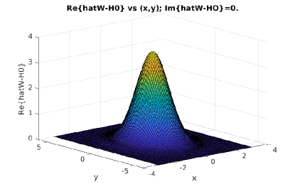
Figure 1: Plot of the real component of the density matrix (in convenient position coordinates) of the harmonic oscillator groundstate (the imaginary component is zero and therefore omitted).

Figure 2: Plot of the real component of the density matrix (in convenient position coordinates) of the steady state for our transformed master equation under a harmonic potential.

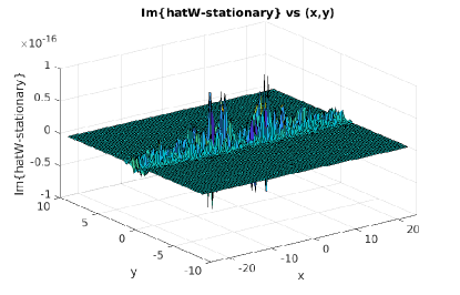
Figure 3: Plot of the imaginary component of the density matrix (in convenient position coordinates) of the steady state for our transformed master equation under a harmonic potential. Notice the low order of magnitude $O(10^{-15})$ versus the real component $O(1)$ one.

The results of our numerical simulations for the time evolution of our transformed master equations by the NIPG DG method are shown below. The time evolution is handled via a theta-method with $\theta=1/2$, as previously indicated. Dirichlet boundary conditions were imposed related to the known analytical solution for the case of a harmonic potential in the numerical solution of this convection-diffusion system. If the domain size is increased, these boundary conditions will converge to homogeneous BC due to Gaussian decay.

The figures below present the projection of our initial condition (the transformed density matrix of the harmonic ground state) into our DG Finite Element (FE) space $V_{h}^{1}$ of piece-wise continuous linear polynomials, for the real and imaginary components of the transformed density matrix in a position basis.

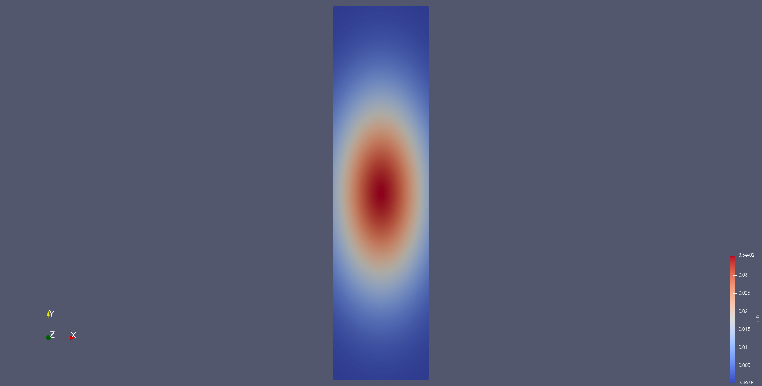
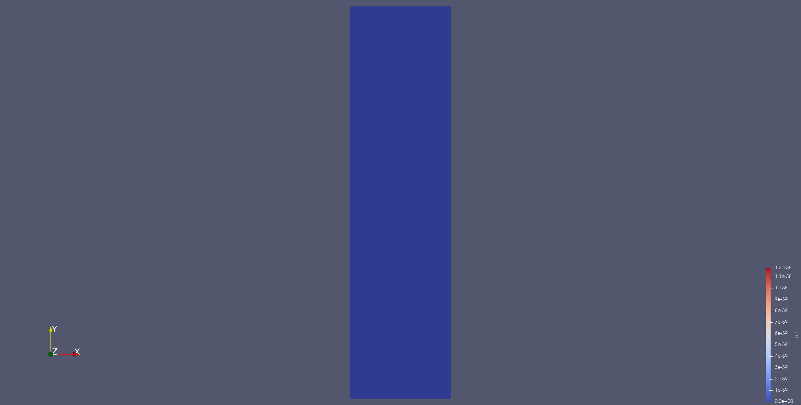
Figure 4: Initial condition for the real (left) and imaginary (right) parts of the density matrix in convenient coordinates, corresponding to a harmonic ground state (projected into the $V_{h}^{1}$ DG FE space). Remark: Color scale differs between right picture and left one.

The numerical steady-state solution for the real and imaginary components of the density matrix is presented as well, which is achieved after a long time (say, a physical time of $50$ in the units of the computational simulation) under the influence of a harmonic potential.

We first present the results for the numerical solution at $t=2$ and then at $t=50$, where in the latter case it is close to the steady state, given our convergence analysis studies to be presented below.

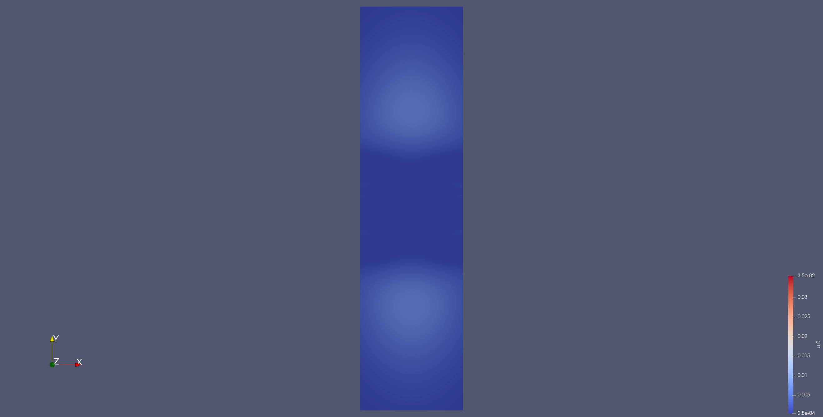
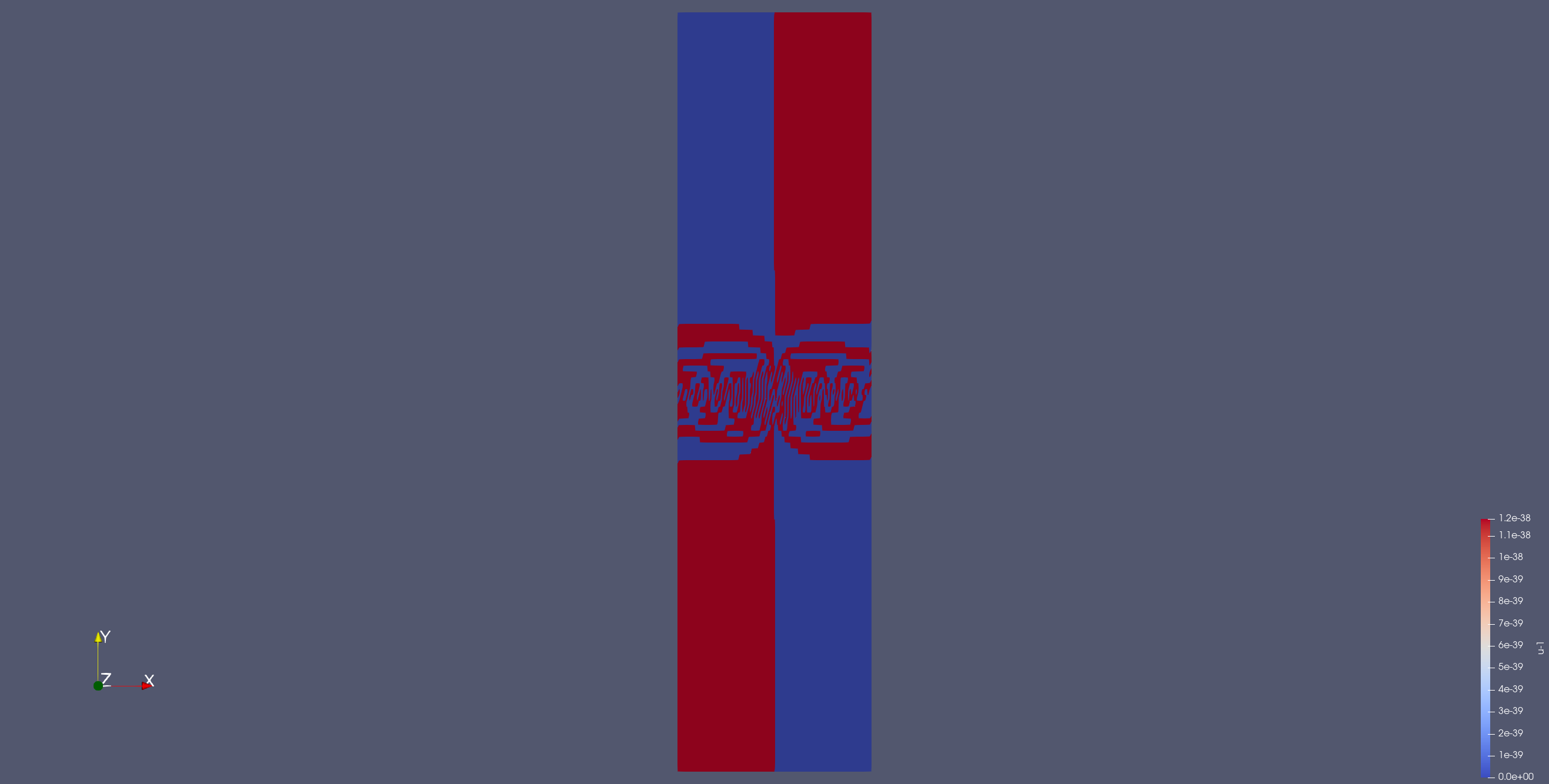
Figure 5: Numerical solution of the real (left) and imaginary (right) parts of the density matrix in convenient coordinates under a harmonic potential after an evolution time of $t=2.0$, solved by NIPG-DG. Remark: Color scale differs between right picture and left one.

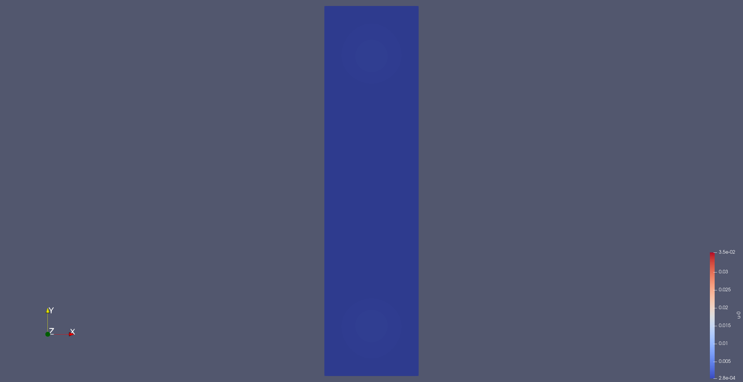
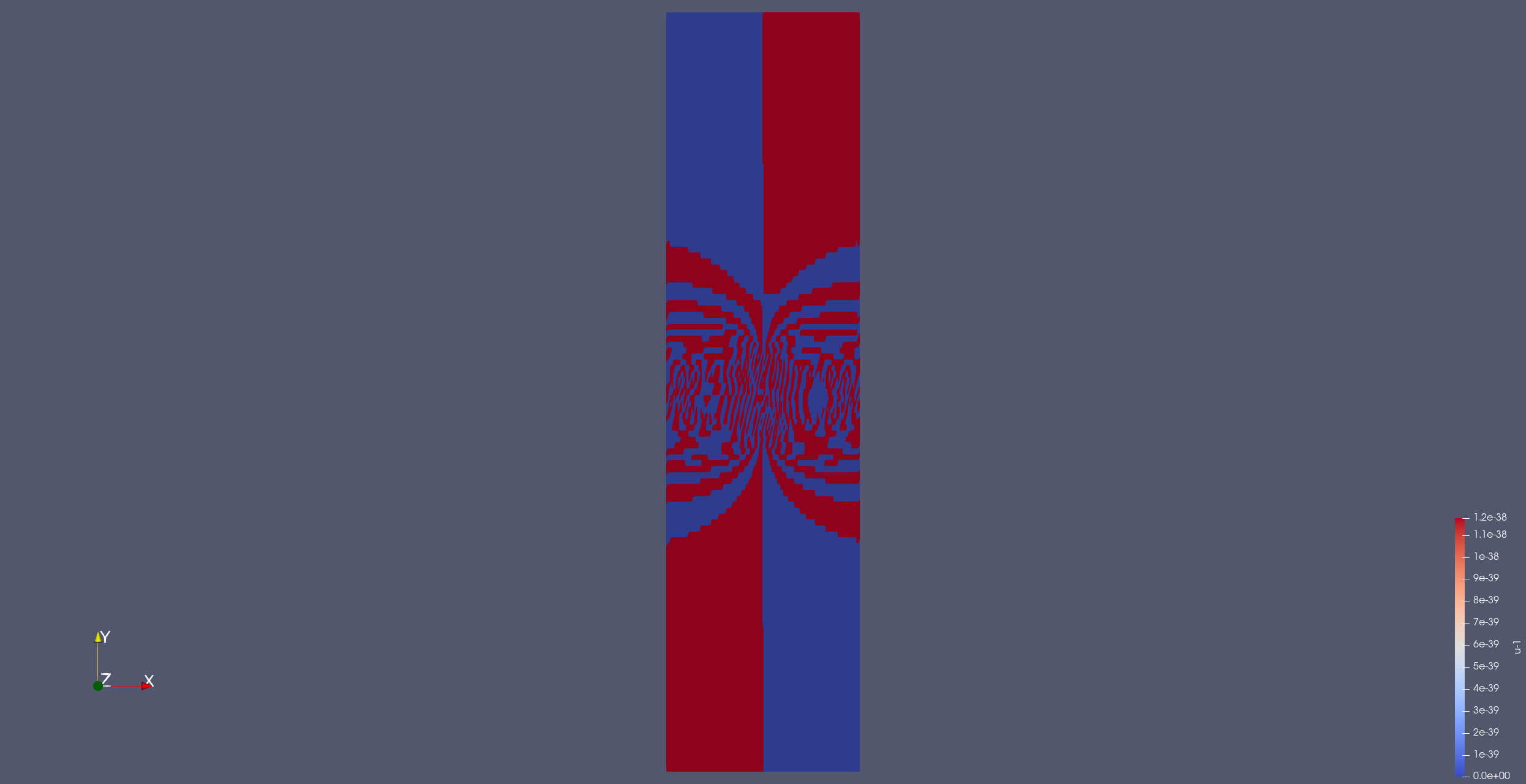
Figure 6: Numerical solution of the real (left) and imaginary (right) parts of the density matrix in convenient coordinates under a harmonic potential after an evolution time of $t=10.0$, solved by NIPG-DG. Remark: Color scale differs between right picture and left one.

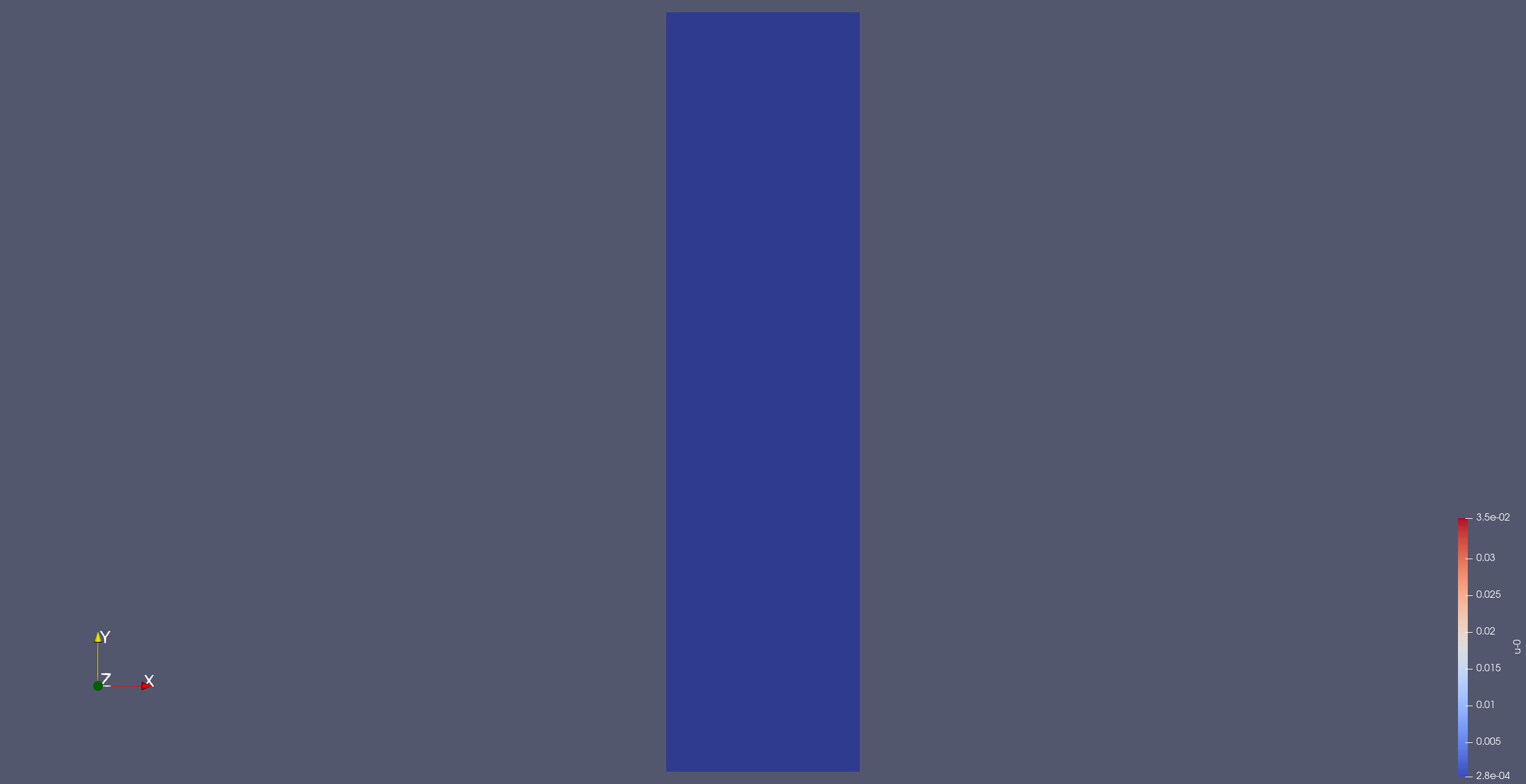
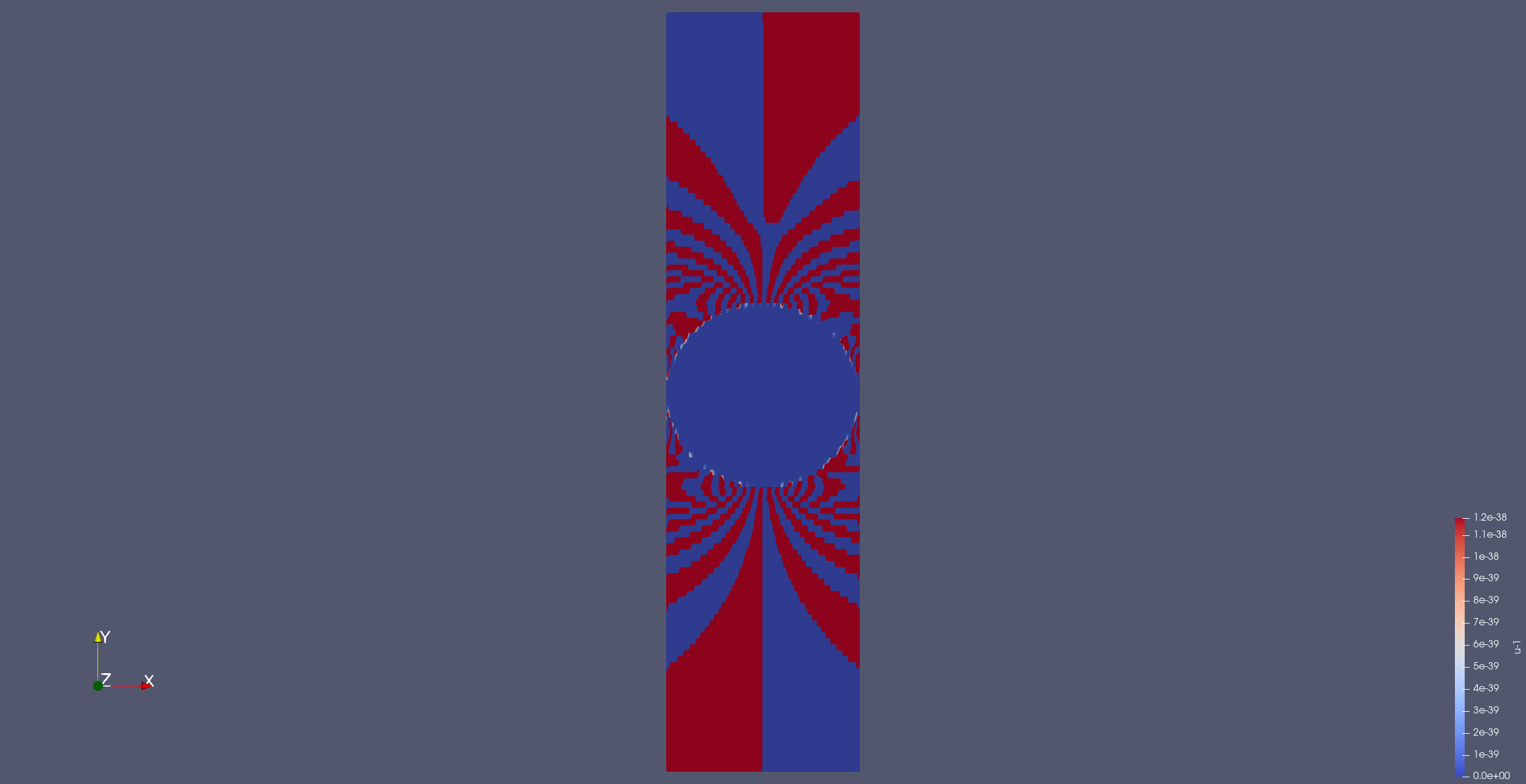
Figure 7: Numerical steady state solution of the real (left) and imaginary (right) parts of the density matrix in convenient coordinates under a harmonic potential after an evolution time of $t=50.0$, solved by NIPG-DG. Remark: Color scale differs between right picture and left one.

5.0.1 Convergence and Error Analysis for NIPG solutions at $t=2.0$

The following table contains the $L_{2}$ error between the analytical steady state solution $u_{\infty}=R_{\infty}+iI_{\infty}$ and the numerical solution $u_{h}|_{t_{f}}=R_{h}|_{t_{f}}+iI_{h}|_{t_{f}}$ achieved after a time of $t_{f}=2.0$ (in normalized units), for both the real and imaginary components of the density matrix in convenient position coordinates. This error is indicated for the different number of intervals in which each dimension is subdivided, with the same number of subdivisions $N_{x}=N_{\eta}$ in $x$ as in $\eta$.

$N_{x}=N=N_{\eta}$	$||R_{\infty}-R_{h}|_{t_{f}}||_{2}$	$||I_{\infty}-I_{h}|_{t_{f}}||_{2}$	$||u_{\infty}-u_{h}|_{t_{f}}||_{2}$
32	4.1992	1.1630	4.3573
64	2.6410	0.7913	2.7570
128	1.0793	0.3235	1.1267

Table 1: Comparison of the $L_{2}$ error in the real and imaginary components of the density matrix between our numerical solution and the known analytical steady state for a harmonic oscillator benchmark problem, under a NIPG solver using a $V_{h}^{1}$ DG FE space, after an evolution time of $t_{f}=2.0$.

The error roughly halves when refining by a factor of 2 the meshing in both $x$ and $\eta$, which is starting to indicate an order of convergence of the method of the type $\varepsilon=O(h^{\kappa}),\,\kappa=1$ (the numerical value that is obtained by the standard fit in the error analysis is $\kappa_{\mathrm{NSfit}}=0.9756$), as piece-wise linear polynomials (degree $\kappa=1$) have been used for our simulations.

For comparison, a table is presented as well where the $L_{2}$ error between the analytical form of the initial condition $u_{0}=R_{0}+iI_{0}$ and its projection $u_{h}|_{t_{0}}=R_{h}|_{t_{0}}+iI_{h}|_{t_{0}}$ into the DG FE space of piece-wise linear polynomials $V_{h}^{1}$ (where $t_{0}=0$) is indicated for the different number of intervals in which each dimension is subdivided, where again $N_{x}=N=N_{\eta}$.

$N_{x}=N=N_{\eta}$	$||R_{0}-R_{h}|_{t_{0}}||_{2}=||u_{0}-u_{h}|_{t_{0}}||_{2}$	$||I_{0}-I_{h}|_{t_{0}}||_{2}$
32	0.0167	0.0
64	0.0042	0.0
128	0.0010	0.0

Table 2: Comparison of the $L_{2}$ projection error in the real and imaginary components of the density matrix in the initial condition between its analytical form and its numerical representation in a $V_{h}^{1}$ DG FE space for NIPG-DG.

In this case, one can observe that the projection error behaves as in $\varepsilon=O(h^{2\kappa}),\,\kappa=1$, using piece-wise linear polynomials. The actual fitted numerical value in the error analysis is $\kappa_{\mathrm{ICfit}}=1.0154$.

A more detailed analysis of the above-mentioned errors is presented below, but now for the case when the number of intervals in $x$ and $\eta$ might differ, for both the projection $L_{2}$ error of the initial condition and the convergence error for the numerical solution versus the steady state after the $t_{f}=2.0$ time.

$||R_{0}-R_{h}|_{t_{0}}||_{2}$	$N_{\eta}=32$	$N_{\eta}=64$	$N_{\eta}=128$
$N_{x}=32$	0.0167	0.0062	0.0039
$N_{x}=64$	0.0150	0.0042	0.0016
$N_{x}=128$	0.0147	0.0038	0.0010

Table 3: Comparison of the $L_{2}$ projection error in the real component (for the imaginary part it is zero) of the density matrix in the initial condition between its analytical form and its numerical representation in a $V_{h}^{1}$ DG FE space for NIPG-DG.

$||R_{\infty}-R_{h}|_{t_{f}}||_{2}$	$N_{\eta}=32$	$N_{\eta}=64$	$N_{\eta}=128$
$N_{x}=32$	4.1992	2.6420	1.0815
$N_{x}=64$	4.1986	2.6410	1.0794
$N_{x}=128$	4.1993	2.6414	1.0793

Table 4: Comparison of the $L_{2}$ error in the real component of the density matrix between our numerical solution and the known analytical steady state for a harmonic oscillator benchmark problem, under a NIPG solver using a $V_{h}^{1}$ DG FE space, after an evolution time of $t_{f}=2.0$.

$||I_{\infty}-I_{h}|_{t_{f}}||_{2}$	$N_{\eta}=32$	$N_{\eta}=64$	$N_{\eta}=128$
$N_{x}=32$	1.1630	0.7872	0.3210
$N_{x}=64$	1.1662	0.7913	0.3227
$N_{x}=128$	1.1678	0.7932	0.3235

Table 5: Comparison of the $L_{2}$ error in the imaginary component of the density matrix between our numerical solution and the known analytical steady state for a harmonic oscillator benchmark problem, under a NIPG solver using a $V_{h}^{1}$ DG FE space, after an evolution time of $t_{f}=2.0$.

The behavior of the $L_{2}$ error regarding the numerical solution after an evolution time of $t_{f}=2.0$ can be explained by understanding that our phenomena is of a convective-diffusive type, where the convective part might dominate over the diffusive one, and since the transport is mostly vertical, the refinement in $\eta$ is the important one regarding error behavior due to mesh discretization, as opposed to the $x$-refinement which doesn’t have as much an effect in changing the aforementioned error.

5.0.2 Convergence and Error Analysis for NIPG solutions at $t=50.0$

The table presented below contains the $L_{2}$ error between the analytical steady state solution $u_{\infty}=R_{\infty}+iI_{\infty}$ and the numerical solution $u_{h}|_{t_{f}}=R_{h}|_{t_{f}}+iI_{h}|_{t_{f}}$ achieved after a time of $t_{f}=50.0$ (where the numerical solution is close to the analytical steady state after that evolution time), for both the real and imaginary components of the density matrix in convenient position coordinates. This error is indicated for the different number of intervals in which each dimension is subdivided, with the same number of subdivisions $N_{x}=N_{\eta}$ in $x$ as in $\eta$.

$N_{x}=N=N_{\eta}$	$||R_{\infty}-R_{h}|_{t_{f}}||_{2}$	$||I_{\infty}-I_{h}|_{t_{f}}||_{2}$	$||u_{\infty}-u_{h}|_{t_{f}}||_{2}$
2	7.2349	0.0283	7.2350
4	5.3768	0.5212	5.4020
8	3.9771	0.8732	4.0718
16	2.2221	0.5987	2.3014
32	0.9311	0.2107	0.9546
64	0.4604	0.0261	0.4612
128	0.3352	0.0246	0.3361

Table 6: Comparison of the $L_{2}$ error in the real and imaginary components of the density matrix in the steady state between our numerical solution and the known analytical one for a harmonic oscillator benchmark problem, under a NIPG solver using a $V_{h}^{1}$ DG FE space, after an evolution time of $t_{f}=50.0$.

The numerical value for the error convergence rate obtained by the standard fit for $||u_{\infty}-u_{h}|_{t_{f}}||_{2}$ is of the type $\varepsilon=O(h^{\kappa}),\,\kappa_{\mathrm{NSfit}}=0.9517$. Let’s remember that piece-wise linear polynomials (degree $\kappa=1$) have been used for our simulations.

For comparison, a table is presented as well where the $L_{2}$ error between the analytical form of the initial condition $u_{0}=R_{0}+iI_{0}$ and its projection $u_{h}|_{t_{0}}=R_{h}|_{t_{0}}+iI_{h}|_{t_{0}}$ into the DG FE space of piece-wise linear polynomials $V_{h}^{1}$ (where $t_{0}=0$) is indicated for the different number of intervals in which each dimension is subdivided, where again $N_{x}=N=N_{\eta}$.

$N_{x}=N=N_{\eta}$	$||R_{0}-R_{h}|_{t_{0}}||_{2}=||u_{0}-u_{h}|_{t_{0}}||_{2}$	$||I_{0}-I_{h}|_{t_{0}}||_{2}$
2	1.4274	0.0
4	0.8582	0.0
8	0.2599	0.0
16	0.0664	0.0
32	0.0167	0.0
64	0.0042	0.0
128	0.0010	0.0

Table 7: Comparison of the $L_{2}$ projection error in the real and imaginary components of the density matrix in the initial condition between its analytical form and its numerical representation in a $V_{h}^{1}$ DG FE space for NIPG-DG.

In this case, one can observe that the projection error behaves as in $\varepsilon=O(h^{2\kappa}),\,\kappa=1$, using piece-wise linear polynomials (the actual fitted numerical value in the error analysis is $\kappa_{\mathrm{ICfit}}=0.9952$).

A more detailed analysis of the above-mentioned errors is presented below, but now for the case when the number of intervals in $x$ and $\eta$ might differ, for both the projection $L_{2}$ error of the initial condition and the convergence error for the numerical solution of the steady state after our evolution time of $t_{f}=50$.

$||R_{0}-R_{h}|_{t_{0}}||_{2}$	$N_{\eta}=8$	$N_{\eta}=16$	$N_{\eta}=32$	$N_{\eta}=64$	$N_{\eta}=128$
$N_{x}=8$	0.2599	0.0982	0.0624	0.0550	0.0534
$N_{x}=16$	0.2348	0.0664	0.0248	0.0157	0.0139
$N_{x}=32$	0.2291	0.0599	0.0167	0.0062	0.0039
$N_{x}=64$	0.2277	0.0584	0.0150	0.0042	0.0015
$N_{x}=128$	0.2273	0.0580	0.0146	0.0037	0.0010

Table 8: Comparison of the $L_{2}$ projection error in the real component (for the imaginary part it is zero) of the density matrix in the initial condition between its analytical form and its numerical representation in a $V_{h}^{1}$ DG FE space for NIPG-DG.

$||R_{\infty}-R_{h}|_{t_{\infty}}||_{2}$	$N_{\eta}=8$	$N_{\eta}=16$	$N_{\eta}=32$	$N_{\eta}=64$	$N_{\eta}=128$
$N_{x}=8$	3.9771	2.2802	0.9567	0.5039	0.3632
$N_{x}=16$	3.8911	2.2221	0.8727	0.4183	0.3004
$N_{x}=32$	3.9393	2.2722	0.9311	0.4764	0.3447
$N_{x}=64$	3.9233	2.2603	0.9151	0.4604	0.3359
$N_{x}=128$	3.9222	2.2591	0.9131	0.4583	0.3352

Table 9: Comparison of the $L_{2}$ error in the real component of the density matrix in the steady state between our numerical solution and the known analytical one for a harmonic oscillator benchmark problem, under a NIPG solver using a $V_{h}^{1}$ DG FE space, after an evolution time of $t_{f}=50.0$.

$||I_{\infty}-I_{h}|_{t_{\infty}}||_{2}$	$N_{\eta}=8$	$N_{\eta}=16$	$N_{\eta}=32$	$N_{\eta}=64$	$N_{\eta}=128$
$N_{x}=8$	0.8732	0.5843	0.2038	0.0252	0.0002
$N_{x}=16$	0.8865	0.5987	0.2085	0.0258	0.0103
$N_{x}=32$	0.8947	0.6056	0.2107	0.0260	0.0235
$N_{x}=64$	0.8993	0.6092	0.2117	0.0261	0.0248
$N_{x}=128$	0.9016	0.6110	0.2122	0.0262	0.0246

Table 10: Comparison of the $L_{2}$ error in the imaginary component of the density matrix in the steady state between our numerical solution and the known analytical one for a harmonic oscillator benchmark problem, under a NIPG solver using a $V_{h}^{1}$ DG FE space, after an evolution time of $t_{f}=50.0$.

The behavior of the $L_{2}$ error regarding the numerical steady state solution can be explained again by understanding that our phenomena is of a convective-diffusive type, but where the convective part dominates over the diffusive one. Since the transport is mostly vertical, the refinement in $\eta$ is the important one regarding error behavior due to mesh discretization, as opposed to the $x$-refinement, which doesn’t seem to have as much an effect again in changing the aforementioned error.

6 Conclusions

Work has been presented regarding the setup of DG numerical schemes applied to a transformed Master Equation, obtained as the Fourier transform of the WFP model for open quantum systems. The Fourier transformation was applied over the WFP equation in order to reduce the computational cost associated with the pseudo-differential integral operator appearing in WFP. The model has been expressed as a system of equations by decomposing it into its real and imaginary parts (when expressing the density matrix in terms of the position basis). Given the $\eta$-transport and $x$-related gradient in the diffusion for this problem, the system has been set up so that an NIPG-DG method can be implemented for the desired numerical solution. Numerical simulations have been presented for the computational study of a benchmark problem such as the case of a harmonic potential, where a comparison between the numerical and analytical steady-state solutions can be performed for a long enough simulation time. Further general potentials could be studied in future work for the analysis of perturbations in an uncertainty quantification setting (or to also consider self-consistent interaction effects between the agents under consideration), as well as the case of $d>1$ for studying the interaction of a system with a noisy environment, as in the Noisy Intermediate Scale Quantum (NISQ) devices regime in higher dimensions $d$.

References

- [1] Alnaes, M.S., Blechta, J., Hake, J., Johansson, A., Kehlet, B., Logg, A., Richardson, C., Ring, J., Rognes, M.E., Wells, G.N.: The FEniCS project version 1.5. Archive of Numerical Software 3 (2015). https://doi.org/10.11588/ans.2015.100.20553
- [2] Alnaes, M.S., Logg, A., Ølgaard, K.B., Rognes, M.E., Wells, G.N.: Unified form language: A domain-specific language for weak formulations of partial differential equations. ACM Transactions on Mathematical Software 40 (2014). https://doi.org/10.1145/2566630
- [3] ARNOLD, A., FAGNOLA, F., NEUMANN, L.: QUANTUM FOKKER-PLANCK MODELS: THE LINDBLAD AND WIGNER APPROACHES, vol. 23, chap. N/A. World Scientific (2008)
- [4] Arnold, A., Ringhofer, C.: An operator splitting method for the wigner-poisson problem. SIAM Journal on Numerical Analysis 33(4), 1622–1643 (1996), http://www.jstor.org/stable/2158320
- [5] D’ARIANO, G., MACCHIAVELLO, C., MORONI, S.: On the monte carlo simulation approach to fokker-planck equations in quantum optics. Modern Physics Letters B 08(04), 239–246 (1994). https://doi.org/10.1142/S0217984994000248, https://doi.org/10.1142/S0217984994000248
- [6] Ferraro, A., Olivares, S., Paris, M.G.A.: Gaussian states in continuous variable quantum information (2005)
- [7] Frensley, W.R.: Boundary conditions for open quantum systems driven far from equilibrium. Rev. Mod. Phys. 62, 745–791 (Jul 1990). https://doi.org/10.1103/RevModPhys.62.745, https://link.aps.org/doi/10.1103/RevModPhys.62.745
- [8] Gamba, I., Gualdani, M.P., Sharp, R.W.: An adaptable discontinuous Galerkin scheme for the Wigner-Fokker-Planck equation. Communications in Mathematical Sciences 7(3), 635 – 664 (2009)
- [9] Ganiu, V., Schulz, D.: Application of discontinuous galerkin methods onto quantum-liouville type equations”, international workshop on computational nanotechnology. International Workshop on Computational Nanotechnology (IWCN) (Jun 2023), https://iwcn2023.uab.es/abstract/67.pdf
- [10] Goudon, T.: Analysis of a semidiscrete version of the wigner equation. SIAM J. Numerical Analysis 40, 2007–2025 (12 2002). https://doi.org/10.1137/S0036142901388366
- [11] Iserles, A.: A First Course in the Numerical Analysis of Differential Equations. Cambridge Texts in Applied Mathematics, Cambridge University Press, 2 edn. (2008). https://doi.org/10.1017/CBO9780511995569
- [12] Jüngel, A.: Transport Equations for Semiconductors. Lecture Notes in Physics, Springer (2009), https://books.google.com/books?id=d6YIyevAQG4C
- [13] Kirby, R.C.: Algorithm 839: FIAT, a new paradigm for computing finite element basis functions. ACM Transactions on Mathematical Software 30, 502–516 (2004). https://doi.org/10.1145/1039813.1039820
- [14] Kirby, R.C.: FIAT: numerical construction of finite element basis functions. In: Logg, A., Mardal, K., Wells, G.N. (eds.) Automated Solution of Differential Equations by the Finite Element Method, Lecture Notes in Computational Science and Engineering, vol. 84, chap. 13. Springer (2012)
- [15] Kirby, R.C., Logg, A.: A compiler for variational forms. ACM Transactions on Mathematical Software 32 (2006). https://doi.org/10.1145/1163641.1163644
- [16] Logg, A., Mardal, K., Wells, G.N., et al.: Automated Solution of Differential Equations by the Finite Element Method. Springer (2012). https://doi.org/10.1007/978-3-642-23099-8
- [17] Logg, A., Wells, G.N.: DOLFIN: automated finite element computing. ACM Transactions on Mathematical Software 37 (2010). https://doi.org/10.1145/1731022.1731030
- [18] Logg, A., Wells, G.N., Hake, J.: DOLFIN: a C++/Python finite element library. In: Logg, A., Mardal, K., Wells, G.N. (eds.) Automated Solution of Differential Equations by the Finite Element Method, Lecture Notes in Computational Science and Engineering, vol. 84, chap. 10. Springer (2012)
- [19] Logg, A., Ølgaard, K.B., Rognes, M.E., Wells, G.N.: FFC: the FEniCS form compiler. In: Logg, A., Mardal, K., Wells, G.N. (eds.) Automated Solution of Differential Equations by the Finite Element Method, Lecture Notes in Computational Science and Engineering, vol. 84, chap. 11. Springer (2012)
- [20] Nielsen, M.A., Chuang, I.L.: Quantum Computation and Quantum Information: 10th Anniversary Edition. Cambridge University Press (2010). https://doi.org/10.1017/CBO9780511976667
- [21] Ringhofer, C.: A spectral method for the numerical simulation of quantum tunneling phenomena. SIAM Journal on Numerical Analysis 27(1), 32–50 (1990), http://www.jstor.org/stable/2157897
- [22] Rivière, B., Wheeler, M.F., Girault, V.: A priori error estimates for finite element methods based on discontinuous approximation spaces for elliptic problems. SIAM Journal on Numerical Analysis 39(3), 902–931 (2002), http://www.jstor.org/stable/3061938
- [23] Scroggs, M.W., Baratta, I.A., Richardson, C.N., Wells, G.N.: Basix: a runtime finite element basis evaluation library. Journal of Open Source Software 7(73), 3982 (2022). https://doi.org/10.21105/joss.03982
- [24] Scroggs, M.W., Dokken, J.S., Richardson, C.N., Wells, G.N.: Construction of arbitrary order finite element degree-of-freedom maps on polygonal and polyhedral cell meshes. ACM Transactions on Mathematical Software (2022). https://doi.org/10.1145/3524456, to appear
- [25] Sparber, C., Carrillo, J., Dolbeault, J., Markowich, P.: On the long-time behavior of the quantum fokker-planck equation. Monatshefte fur Mathematik 141(3), 237–257 (Mar 2004). https://doi.org/10.1007/s00605-003-0043-4
- [26] Suh, N.D., Feix, M.R., Bertrand, P.: Numerical simulation of the quantum liouville-poisson system. Journal of Computational Physics 94, 403–418 (1991), https://api.semanticscholar.org/CorpusID:120155444
- [27] Ølgaard, K.B., Wells, G.N.: Optimisations for quadrature representations of finite element tensors through automated code generation. ACM Transactions on Mathematical Software 37 (2010). https://doi.org/10.1145/1644001.1644009