More on the tensionless limit of pure-Ramond-Ramond AdS3/CFT2

Abstract

In a recent letter we presented the equations which describe tensionless limit of the excited-state spectrum for strings on $AdS_{3}\times S^{3}\times T^{4}$ supported by Ramond-Ramond flux, and their numerical solution. In this paper, we give a detailed account of the derivation of these equations from the mirror TBA equations proposed by Frolov and Sfondrini, discussing the contour-deformation trick which we used to obtain excited-state equations and the tensionless limit. We also comment at length on the algorithm for the numerical solution of the equations in the tensionless limit, and present a number of explicit numerical results, as well as comment on their interpretation.

1 Introduction

An important family of string backgrounds in the AdS3/CFT2 holographic correspondence Maldacena:1997re involves the $\text{AdS}_{3}\times\text{S}^{3}\times\text{T}^{4}$ geometry and supports 16 Killing spinors — the maximal amount for an $\text{AdS}_{3}$ background Haupt:2018gap . This is a family of backgrounds as it depends on several moduli, see Larsen:1999uk ; OhlssonSax:2018hgc for a detailed description. A very intriguing one-parameter family of supergravity backgrounds is the one interpolating between the case with no Kalb-Ramond $B$-field (but with Ramond-Ramond background fluxes) and the one with no RR fluxes (but with a $B$-field). In supergravity this is a continuous interpolation, but in string theory the coefficient $k$ of the $B$-field has to be quantised. In perturbative string theory, which will be our focus here, the string coupling $g_{s}$ is vanishingly small, while the string tension is sourced by both $k$ and by the RR coupling $g$,

$$T=\frac{R^{2}}{2\pi\,\alpha^{\prime}}=\sqrt{\frac{k^{2}}{4\pi^{2}}+g^{2}}\,,\qquad k\in\mathbb{N}_{0}\,,\qquad g\geq 0\,.$$ (1)

Here $R$ is the radius of the of the three-sphere, which is equal to the radius of $\text{AdS}_{3}$.

By far the best understood setup in this duality is the case in which $g=0$ and $k=1,2,3,\dots$. Then, the model can be described as worldsheet CFT, namely a supersymmetric Wess-Zumino-Novikov-Witten model Giveon:1998ns , and it can be solved Maldacena:2000hw . In particular, the free-string spectrum can be worked out explicitly and it features a discrete set of (highly degenerate) states, as well as a continuum. This knowledge of the spectrum allowed to conjecture the dual of these string backgrounds, which are believed to take the form of symmetric-product orbifold CFTs Giribet:2018ada ; Eberhardt:2018ouy ; Eberhardt:2021vsx . Of these, the simplest and best understood is the symmetric-product orbifold of $T^{4}$, (meaning, of four free bosons with $\mathcal{N}=(4,4)$ supersymmetry), which is dual to the $g=0$, $k=1$ string theory.

Things are significantly more involved for $g>0$, i.e. when turning on RR-background fields (which can be done by tuning the RR scalar $C_{0}$, see OhlssonSax:2018hgc ). In this case, the worldsheet CFT becomes nonlocal Berenstein:1999jq ; Cho:2018nfn , and it is hard to decouple its ghost sector Berkovits:1999im ; Eberhardt:2018exh . Qualitatively, we expect the continuum part of the spectrum to disappear and the degeneracies in the discrete spectrum to lift — aside of course from the ones due to superconformal symmetry. The polar opposite of the WZNW setup is the case where $k=0$ (i.e., there is no $B$-field at all) and the tension (1) is entirely sourced by the RR fluxes. This case is qualitatively similar to that of strings on $\text{AdS}_{5}\times\text{S}^{5}$ or on $\text{AdS}_{4}\times\text{CP}^{3}$, and indeed we expect the spectrum to be as nontrivial as the one of a planar gauge theory. Even in such complicated cases, not all hope is lost as integrability can be exploited to understand the planar spectrum, see Arutyunov:2009ga ; Beisert:2010jr for reviews. One may hope that the same is true for $\text{AdS}_{3}$ backgrounds too, and this turns out to be true, see Sfondrini:2014via .

More specifically, the Green-Schwarz action $\text{AdS}_{3}\times\text{S}^{3}\times\text{T}^{4}$ with generic $k$ and $g$ is classically integrable Cagnazzo:2012se , and there is good evidence that integrability persists at the quantum level too, in terms of factorised scattering on the worldsheet. Moreover, the integrability construction is particularly robust in the case of $g>0$ and $k=0$. In this case, the construction of the integrable S matrix has been recently completeted by a proposal for the dressing factors Frolov:2021fmj . This allowed to derive the mirror TBA equations Frolov:2021bwp which describe the whole planar spectrum of the theory (for arbitrary values of the tension $g$). This provides us with the possibility of making quantitative predictions for pure-RR $\text{AdS}_{3}\times\text{S}^{3}\times\text{T}^{4}$ strings. This is the main aim of this paper.

It is generally the case that the TBA equations cannot be solved in closed-form for generic unprotected states, and that each family of states (differing by the number of asymptotic worldsheet excitations) require a separate analysis. For this reason, here we focus on a subset of states, i.e. those that acquire an anomalous dimension at low tension $T\ll 1$. This is the limit where the dual-CFT description, whatever it may be, should simplify significantly. For instance, in this limit in $\text{AdS}_{5}\times\text{S}^{5}$ one recovers a nearest-neighbour integrable spin-chain Minahan:2002ve . It is natural to ask whether in our case we may find some similar spin chain, or a free CFT (like the symmetric-product orbifold of $\text{T}^{4}$), or something else entirely. In this paper we will not be able to construct the dynamics (i.e., the Hamiltonian) in the $T\ll 1$ regime, but only to read off the spectrum. This will still be sufficient to rule out some otherwise believable scenarios.

The main results of this paper were presented in short form elsewhere Brollo:2023pkl . As outlined there, our strategy is to start from the full, nonperturbative equations of Frolov:2021bwp , appropriately modified to described excited states, and expand them at small tension. The equations depend on a parameter $h(T)$ which at small tension can be identified with $T$ itself,

$$h(T)\sim T=g\,,\qquad T\ll 1\,.$$ (2)

In what follows, in analogy with the notation of the existing literature, we will indicate the parameter as $h$. From the small-$h$ expansion we will find a set of equations which we will solve numerically to high precision.

This paper is structured as follows. In section 2 we briefly review the model and in section 3 we recap the mirror TBA equations for the ground state. In section 4 we derive the equations for excited states through the contour-deformation trick; we focus on massless excitations, which are leading at small tension. In section 5 we take the small-tension limit and show that several of the mirror TBA equations decouple. In section 6 we further simplify and summarise the small-tension TBA equations. Finally, in section 7 we discuss their numerical solution and present the results, and we conclude in section 8. We also include some further details in appendices. Appendix A summarises our notation. Appendix B discusses some identities of the integration kernels which we need to simplify the TBA equations. Appendix C proves some of the identities that we use in the weak-tension expansion of the TBA equations, while appendix D contains a detailed discussion of the Beisert-Eden-Staudacher phase in various regimes (in the massive and massless kinematics). In appendix E we discuss in more detail the large-volume behaviour of the mirror TBA equations. Finally, appendix F contains several tables containing numeric results.

2 Particle Content and Kinematics

Let us begin by briefly reviewing the model of interest. Strings on $\text{AdS}_{3}\times\text{S}^{3}\times\text{T}^{4}$ with RR flux feature infinitely many worldsheet excitations, labelled by a number $m\in\mathbb{Z}$, with periodic momentum $p$ and energy Lloyd:2014bsa

$$\mathcal{E}(p)=\sqrt{m^{2}+4h^{2}\sin^{2}(p/2)}\,,$$ (3)

where $h$ is the coupling constant. In the mirror model, the dispersion relation becomes

$$\widetilde{\mathcal{E}}(\tilde{p})=2\,\text{arcsinh}\left(\frac{\sqrt{m^{2}+\tilde{p}^{2}}}{2h}\right)\,.$$ (4)

Notice that, for $m=0$, both dispersion relations have no mass gap. Strictly speaking, this dispersion relation applies to a whole supermultiplet of particles, which takes a different form in the string and mirror model, see Seibold:2022mgg . Notably, in either case, the dimension of the representation does not grow with $|m|$, but it is fixed to being four-dimensional (this is unlike what happens, for instance, in $\text{AdS}_{5}\times\text{S}^{5}$).

When analysing the mirror model in the thermodynamic limit, we identify the following type of particles:

• $Q$-particles. These are essentially bound states with $Q=m=1,2,\dots$.

• $\overline{Q}$-particles. These are essentially bound states with $\overline{Q}=-m=1,2,\dots$.

• Massless particles, which we also indicate with $Q=0$. These are the modes with $m=0$, and come in two copies, labelled by an index $\dot{\alpha}=1,2$. In the literature, this index is associated with the so call $\mathfrak{su}(2)_{\circ}$ which is part of the $\mathfrak{so}(4)$ acting geometrically on the four flat directions. We will slightly generalise this construction, and allow the index $\dot{\alpha}$ to run from $1$ to $N_{0}$, without specifying that $N_{0}=2$ until the very end. This will allow us, later on, to discuss a very recent proposal for the TBA equations Frolov:2023wji .

• Auxiliary particles, which account for the supermultiplet structure of the various bound-state representations and do not contribute to the energy. They are labelled by an index $\alpha=1,2$ (without dot), related to the $\mathfrak{su}(2)_{\bullet}$ which also comes from the $\mathfrak{so}(4)$ acting geometrically on the four flat directions, $\mathfrak{so}(4)\cong\mathfrak{su}(2)_{\bullet}\oplus\mathfrak{su}(2)_{\circ}$. Later on, we will attach a further index $\pm$ to these auxiliary roots, which will make it easier to parametrise them (just like it is done in $\text{AdS}_{5}\times\text{S}^{5}$ Arutyunov:2009zu ).

It is worth emphasising that, unlike what happens in $\text{AdS}_{5}\times\text{S}^{5}$, there are no Bethe strings involving fundamental particles and auxiliary roots. This is because the dimension of the bound state representation does not grow with $Q$ or $\overline{Q}$.

Finally, we stress that this construction, which is the one of Frolov:2021bwp , relies on the scattering between massless representations with different $\mathfrak{su}(2)_{\circ}$ quantum number being trivial. This is what seems to appear from comparison with perturbative computations, see the discussions of Lloyd:2014bsa . Were we to allow for a non-trivial $\mathfrak{su}(2)_{\circ}$ S matrix, we would obtain a different string hypothesis. This is discussed in toappear .

2.1 String-region parametrisation

It is convenient to introduce suitable variables to parametrise the momentum and energy in the string and mirror models.

In the string region we can introduce Zhukovsky variables satisfying, for $m\neq 0$,

$$\frac{x^{+}}{x^{-}}=e^{ip},\qquad\frac{h}{2i}\left(x^{+}-\frac{1}{x^{+}}-x^{-}+\frac{1}{x^{-}}\right)=\mathcal{E}(p)\,,$$ (5)

subject to the constraint

$$\frac{h}{2i}\left(x^{+}+\frac{1}{x^{+}}-x^{-}-\frac{1}{x^{-}}\right)=|m|\,.$$ (6)

For the special case $m=0$, we have

$$x_{s}\equiv x^{+}=\frac{1}{x^{-}}\,,\qquad(m=0)\,.$$ (7)

Hence $(x_{s})^{2}=e^{ip}$ and we take $x$ to lie on the upper half-circle for particles of real momentum. It is convenient to solve the constraint (6) in terms of an unconstrained variable $u$

$$u=x^{+}+\frac{1}{x^{+}}-\frac{i|m|}{h}=x^{-}+\frac{1}{x^{-}}+\frac{i|m|}{h}=x+\frac{1}{x}\,.$$ (8)

In the string region we may solve this relation by defining

$$x_{s}(u)=\frac{u}{2}\left(1+\sqrt{1-\frac{4}{u^{2}}}\right)\,,$$ (9)

which has cuts for $-2\leq u\leq+2$, and letting

$$x^{\pm}(u)=x_{s}(u\pm\tfrac{i}{h}|m|)\,.$$ (10)

For massive particles with real momenta, the rapidities take values on the real line. In the massless case $m=0$, this formula should be understood as a “$\pm i0$” prescription at the cut $-2\leq u\leq+2$, which fits with (7). In particular, in eq. (7), $x=x_{s}(u+i0)$ with $-2\leq u\leq+2$. It is also useful to introduce the following $\gamma$-parametrisation Frolov:2021fmj , see also Fontanella:2019baq ,

$$x^{\pm}=\frac{i\mp e^{\gamma^{\pm}}}{i\pm e^{\gamma^{\pm}}}\,.$$ (11)

To invert this relation we need to pick a branch, and we choose in the string region Frolov:2021fmj

$$\gamma^{\pm}=\ln\left(\mp i\frac{x^{\pm}-1}{x^{\pm}+1}\right)\,.$$ (12)

Note that with these choices we have the following reality conditions for real-momentum particles in the string region:

$$(x^{+})^{*}=x^{-}\,,\qquad(\gamma^{+})^{*}=\gamma^{-}\,.$$ (13)

Analogously, for massless particles we set

$$x_{s}(\gamma_{s})=\frac{i-e^{\gamma_{s}}}{i+e^{\gamma_{s}}}\,,\qquad\gamma_{s}(x_{s})=\ln\left(-i\frac{x_{s}-1}{x_{s}+1}\right)\,,$$ (14)

with the reality conditions, for real-momentum particles in the string model

$$(x_{s})^{*}=\frac{1}{x_{s}}\,,\qquad(\gamma_{s})^{*}=\gamma_{s}\,,$$ (15)

where the subscript “$s$” emphasises that we are discussing the string model (this is to avoid clashes with later notation).

2.2 Mirror-region parametrisation

In this paper we will be chiefly interested in the mirror model, which is related to the string model by analytic continuation Arutyunov:2007tc ; Frolov:2021zyc . In this case we introduce the (mirror) Zhukovsky parametrisation

$$x(u)=\frac{1}{2}\left(u-i\sqrt{4-u^{2}}\right)$$ (16)

which has cuts on the real $u$-line for $|u|>2$. For massive particles we write

$$x^{\pm}(u)=x(u\pm\tfrac{i}{h}Q)\,,\qquad x^{\pm}(u)=x(u\pm\tfrac{i}{h}\overline{Q})\,,$$ (17)

For massless particles, like before, this means

$$x(u)=x(u+i0)=\frac{1}{x(u-i0)}\,.$$ (18)

Now $u$ is on the real $u$-line with $|u|>2$, and $x(u+i0)$ lies on the interval $-1\leq x\leq 1$ on the real axis. In the mirror region the momentum for a $Q$-particle is given by

$$\tilde{p}^{Q}(u)=h\left(x(u-\tfrac{i}{h}Q)-x(u+\tfrac{i}{h}Q)\right)+iQ\,,$$ (19)

while the mirror energy for a $Q$-particle is

$$\tilde{\mathcal{E}}^{Q}(u)=\ln\frac{x(u-\frac{i}{h}Q)}{x(u+\frac{i}{h}Q)}\,,$$ (20)

where we made the $Q$-dependence explicit for later convenience. The formulae for $\overline{Q}$-particles are identical. For $Q=0$ we have

$$\tilde{\mathcal{E}}^{0}(u)=-\ln\left(x(u+i0)\right)^{2}\,.$$ (21)

Note that this function is not analytic, see also Frolov:2021zyc . We will discuss its branches in Section 2.3. It can be checked that, with these definitions, we reproduce the mirror dispersion relation (4) with $|m|=Q$ or $|m|=\overline{Q}$. Let us emphasise that real-momentum particles are defined for

• $u\in\mathbb{R}$ for $Q$ and $\overline{Q}$ particles,

• $u\in(-\infty,-2)\cup(+2,+\infty)$ for massless particles.

The relation between the $\gamma$-parameter in the mirror theory satisfies, for massless mirror particles,

$$x(\gamma)=-\tanh\frac{\gamma}{2}\,,\qquad\gamma(x)=-2\,\text{atanh}(x)\,,$$ (22)

so that

$$\gamma(u)=\gamma(x(u))=\frac{1}{2}\ln\left(-\frac{u-2}{u+2}\right)+\frac{i\pi}{2}\,.$$ (23)

Using this formula we can define for $Q$-particles (or $\overline{Q}$-particles),

$$\gamma^{-}(u)=\gamma(u-\tfrac{i}{h}Q),\qquad\gamma^{+}(u)=\gamma(u+\tfrac{i}{h}Q)-i\pi\,.$$ (24)

The reality conditions in the mirror theory are, for real-mirror-momentum particles,

$$(x^{\pm})^{*}=\frac{1}{x^{\mp}}\,,\qquad(\gamma^{\pm})^{*}=\gamma^{\mp}\,,$$ (25)

and

$$x^{*}=x\,,\qquad\gamma^{*}=\gamma\,,$$ (26)

where in these two last formulae it is necessary to correctly account for the branch cut on real $u$, $|u|>2$. Finally, by directly comparing this definition of $\gamma$ with the one given in the string region we see that

$$\gamma(u)\Big{|}_{\text{string}}=\gamma(u)\Big{|}_{\text{mirror}}-\frac{i\pi}{2}\,,$$ (27)

where $\gamma(u)_{\text{mirror}}$ is defined by (23) and $\gamma(u)_{\text{string}}=\gamma(x_{s}(u))$. In what follows, we will indicate the latter by $\gamma_{s}$, so that when treating $\gamma$ as a free variable we will write

$$\gamma_{s}=\gamma-\frac{i\pi}{2}\,.$$ (28)

The inverse of $\gamma(u)$ is given by

$$u(\gamma) =-2\coth(\gamma), u\in(-\infty,-2)\cup(2,\infty)$$ (29)

$$u_{s}(\gamma_{s}) =-2\tanh(\gamma_{s}), u_{s}\in(-2,2).$$

If $u$ is slightly above the real axis, $\gamma$ is found at:

$$u+i0\ \ \leftrightarrow\ \ \gamma+i0,\qquad u_{s}+i0\ \ \leftrightarrow\ \ \gamma_{s}-i0.$$ (30)

Neither $u(\gamma)$ nor $u_{s}(\gamma_{s})$ covers the whole real line.

2.3 Explicit formulae for massless particles

In what follows the kinematics of the massless particles will be particularly important. Let us spell out explicitly the parametrisation of various physical quantities in terms of the $\gamma$ and $\gamma_{s}$ rapidities. In the string theory we have

$$\mathcal{E}_{0}=\frac{2h}{\cosh\gamma_{s}}\,,\qquad p_{0}=-i\ln\left(\frac{i-e^{\gamma_{s}}}{i+e^{\gamma_{s}}}\right)^{2},$$ (31)

where the branches of $\log z^{2}$ can be resolved as

$$p^{0}=\begin{cases}-2i\ln\left(+\frac{i-e^{\gamma_{s}}}{i+e^{\gamma_{s}}}\right),\qquad&\gamma_{s}>0\quad(-\pi\leq p\leq 0),\\ -2i\ln\left(-\frac{i-e^{\gamma_{s}}}{i+e^{\gamma_{s}}}\right),\qquad&\gamma_{s}<0\quad(0\leq p\leq+\pi).\end{cases}$$ (32)

The necessity of picking different branches for positive and negative momentum is a consequence of the gapless dispersion relation and it was discussed at length in Frolov:2021zyc . For mirror particles we have, for $\gamma$ slightly above the real axis,

$$\tilde{p}_{0}=-\frac{2h}{\sinh\gamma}\,,\qquad\widetilde{\mathcal{E}}_{0}=-\ln\left(\frac{1-e^{\gamma}}{1+e^{\gamma}}\right)^{2}\,.$$ (33)

Again we can resolve the branches of the logarithm as Frolov:2021zyc

$$\widetilde{\mathcal{E}}_{0}=\begin{cases}-2\ln(\frac{1-e^{\gamma}}{1+e^{\gamma}})+2\pi i,\qquad&\gamma>0\quad(\tilde{p}^{0}<0),\\ -2\ln(\frac{1-e^{\gamma}}{1+e^{\gamma}}),\qquad&\gamma<0\quad(\tilde{p}^{0}>0),\end{cases}$$ (34)

where the variables take values just above the real-$\gamma$ line.

2.4 Parametrisation of (mirror) auxiliary particles

Let us finally briefly discuss the parametrisation of the auxiliary particles. In this work, we will only need their kinematics in the mirror theory. In Frolov:2021bwp it was argued that, for the Bethe-Yang equations of the mirror model to admit a solution, the rapidity variable of the auxiliary particles must lie on the unit circle. Hence, we have that quite curiously the mirror kinematics of auxiliary particles is the same as the string kinematics of massless particles (see (15) for the string massless kinematics). One important difference is that auxiliary particles can take values on either the upper or lower half-circle — not just the upper, like for string massless particles. (Another difference is that there is no momentum or energy associated to the auxiliary particles.) Therefore we will define two types of auxiliary “particles”:

• $y^{-}$ particles, whose rapidity is parametrised by $x(u)$ with $-2<u<+2$, which parametrise the lower half-circle; equivalently, we can use $x_{s}(u-i0)$.

• $y^{+}$ particles, whose rapidity is parametrised by $1/x(u)$ with $-2<u<+2$, which parametrise the upper half-circle; equivalently, we can use $x_{s}(u+i0)$.

In terms of the $\gamma$ variable therefore we can use the string parametrisation (14).

3 Ground-state mirror TBA equations

Let us collect here the ground-state TBA equations which were derived in Frolov:2021bwp for the mirror model. The equations are written in the $u$-variables introduced above, and all quantities are in the mirror kinematics. The domain of $u$ is chosen to cover all real values of momentum — or, in case of the auxiliary particles, the unit circle of the Zhukovsky plane. The various kernels appearing in the equations below are defined as the logarithmic derivatives of appropriate S matrices in the mirror-mirror kinematics. Schematically,

$$K(u,u^{\prime})=\frac{1}{2\pi i}\frac{\text{d}}{\text{d}u}\log{S(u,u^{\prime})}\,.$$ (35)

The precise form of the various S matrices and kernels is collected in appendix A. We will use the short-hand notation

$$\rho_{j}\star K_{ji}(u)=\sum_{j}\int\text{d}u^{\prime}\rho_{j}(u^{\prime})K_{ji}(u^{\prime},u)\,.$$ (36)

When writing the convolutions, we use

$$\star\leftrightarrow\int\limits_{-\infty}^{+\infty}\text{d}u,\qquad\hat{\star}\leftrightarrow\int\limits_{-2}^{+2}\text{d}u,\qquad\check{\star}\leftrightarrow\int\limits_{-\infty}^{-2}\text{d}u+\int\limits_{+2}^{+\infty}\text{d}u\,.$$ (37)

In particular, in view of the discussion in the previous section, we will use the convolutions

• “$\star$” for $Q$ and $\overline{Q}$ particles,

• “$\hat{\star}$” for auxiliary particles,

• “$\check{\star}$” for massless particles.

We will later rewrite the kernels and TBA equations in terms of the $\gamma$ variables, and introduce ad hoc symbols for kernels and convolutions.

It is worth emphasising a potential ambiguity in the derivation of the mirror TBA equations — whether certain expressions should be understood as sum of logarithms, or logarithms of products. For the time being, we will not specify the branch of the logarithm. We will address this ambiguity later on.

3.1 Mirror TBA equations

The equations are written in terms of $Y$-functions. We have Frolov:2021bwp :

Equations for $Q$-particles.

$$-\log Y_{Q} =L\tilde{\mathcal{E}}_{Q}-\log{(1+Y_{Q^{\prime}})}\star K_{\textit{sl}}^{Q^{\prime}Q}-\log{(1+\bar{Y}_{Q^{\prime}})}\star\tilde{K}_{\textit{su}}^{Q^{\prime}Q}$$ (38)

$$-\sum_{\dot{\alpha}=1}^{N_{0}}\log{(1+Y_{0}^{(\dot{\alpha})})}\check{\star}K^{0Q}$$

$$-\sum_{\alpha=1,2}\log{\left(1-\frac{1}{Y_{+}^{(\alpha)}}\right)}\hat{\star}K_{+}^{yQ}-\sum_{\alpha=1,2}\log{\left(1-\frac{1}{Y_{-}^{(\alpha)}}\right)}\hat{\star}K_{-}^{yQ}\,.$$

Equations for $\bar{Q}$-particles.

$$-\log\bar{Y}_{Q} =L\tilde{\mathcal{E}}_{Q}-\log{(1+\bar{Y}_{Q^{\prime}})}\star K_{\textit{su}}^{Q^{\prime}Q}-\log{(1+Y_{Q^{\prime}})}\star\tilde{K}_{\textit{sl}}^{Q^{\prime}Q}$$ (39)

$$-\sum_{\dot{\alpha}=1}^{N_{0}}\log{(1+Y_{0}^{(\dot{\alpha})})}\check{\star}\tilde{K}^{0Q}$$

$$-\sum_{\alpha=1,2}\log{\left(1-\frac{1}{Y_{+}^{(\alpha)}}\right)}\hat{\star}K_{-}^{yQ}-\sum_{\alpha=1,2}\log{\left(1-\frac{1}{Y_{-}^{(\alpha)}}\right)}\hat{\star}K_{+}^{yQ}\,.$$

Equations for Massless particles.

​​​​​​

$$-\log Y_{0}^{(\dot{\alpha})} =L\tilde{\mathcal{E}}_{0}-\sum_{\dot{\beta}=1}^{N_{0}}\log{(1+Y_{0}^{(\dot{\beta})})}\check{\star}K^{00}-\log{(1+Y_{Q})}\star K^{Q0}-\log{(1+\bar{{Y}_{Q}})}\star\tilde{K}^{Q0}$$ (40)

$$-\sum_{\alpha=1,2}\log{\left(1-\frac{1}{Y_{+}^{(\alpha)}}\right)}\hat{\star}K^{y0}-\sum_{\alpha=1,2}\log{\left(1-\frac{1}{Y_{-}^{(\alpha)}}\right)}\hat{\star}K^{y0}\,.$$

Equation for auxiliary $y^{-}$-particles.

$$\log{Y_{-}^{(\alpha)}}=-\log{(1+Y_{Q})}\star K_{-}^{Qy}+\log{(1+\bar{Y}_{Q})}\star K_{+}^{Qy}+\sum_{\dot{\alpha}=1}^{N_{0}}\log{(1+Y_{0}^{(\dot{\alpha})})}\check{\star}K^{0y}\,.$$ (41)

Equation for auxiliary $y^{+}$-particles.

$$\log{Y_{+}^{(\alpha)}}=-\log{(1+Y_{Q})}\star K_{+}^{Qy}+\log{(1+\bar{Y}_{Q})}\star K_{-}^{Qy}-\sum_{\dot{\alpha}=1}^{N_{0}}\log{(1+Y_{0}^{(\dot{\alpha})})}\check{\star}K^{0y}\,.$$ (42)

3.2 Energy and momentum

Once the Y-functions are determined, it is possible to compute the (ground-state) energy by the following formula:

$$E(L)= -\int\limits_{-\infty}^{\infty}\frac{\text{d}u}{2\pi}\frac{\text{d}\tilde{p}^{Q}}{\text{d}u}\log{\left((1+Y_{Q})(1+\bar{Y}_{Q})\right)}$$ (43)

$$-\int\limits_{|u|>2}\frac{\text{d}u}{2\pi}\frac{\text{d}\tilde{p}^{0}}{\text{d}u}\sum_{\dot{\alpha}=1}^{N_{0}}\log{\left(1+Y_{0}^{(\dot{\alpha})}\right)}\,.$$

Note that auxiliary Y-functions do not contribute to the formula. It is also useful to write a similar formula to impose that the total-momentum of the (ground) state vanishes, namely

$$0= -\int\limits_{-\infty}^{\infty}\frac{\text{d}u}{2\pi}\frac{\text{d}\tilde{\mathcal{E}}_{Q}}{\text{d}u}\log{\left((1+Y_{Q})(1+\bar{Y}_{Q})\right)}$$ (44)

$$-\int\limits_{|u|>2}\frac{\text{d}u}{2\pi}\frac{\text{d}\tilde{\mathcal{E}}_{0}}{\text{d}u}\sum_{\dot{\alpha}=1}^{N_{0}}\log{\left(1+Y_{0}^{(\dot{\alpha})}\right)}\,.$$

This is the level-matching condition in string theory (in a sector without winding around the lightcone, see Arutyunov:2009ga ).

4 Exciting the massless modes

Let us now discuss how the ground-state equations change if we consider states containing massless excitations. This can be done by the contour-deformation trick of Dorey and Tateo Dorey:1996re . For simplicity, we consider only states involving an even number of massless modes with real momenta coming in pairs, $(p_{j},-p_{j})$, and without any auxiliary excitations. As it will become clear in a moment, this will ensure that the $Y$-functions are symmetric under $u\to-u$ and, in turn, that the level-matching condition is satisfied.

4.1 Contour-deformation trick

We expect the equations to be modified by “driving terms” which arise out of the contour-deformation trick. They come from picking up residues in the various convolution in places where

$$Y_{0,\text{string}}^{(\dot{\alpha}_{j})}\big{(}u_{j}^{\dot{\alpha}_{j}}\big{)}=-1\,,\qquad j=1,\dots 2M\,.$$ (45)

The subscript “string” reminds us that the values $u_{j}^{\dot{\alpha}_{j}}$ where this may happen lie in the string, rather than mirror, region. In fact, for the case at hand, this will happen when $u_{j}^{\dot{\alpha}_{j}}$ is on the real-string line for massless particles. We indicate with an asterisk the S-matrix elements which have one leg in the string-region. Furthermore, we indicated by a dot the free argument of each functional equation (which takes value on the real mirror line). Formally, we find a simple modification of the equations, written in blue.

Equations for $Q$-particles.

$$-\log Y_{Q} =L\tilde{\mathcal{E}}_{Q}-\log{(1+Y_{Q^{\prime}})}\star K_{\textit{sl}}^{Q^{\prime}Q}-\log{(1+\bar{Y}_{Q^{\prime}})}\star\tilde{K}_{\textit{su}}^{Q^{\prime}Q}$$ (46)

$$-\sum_{\dot{\alpha}=1}^{N_{0}}\log{(1+Y_{0}^{(\dot{\alpha})})}\check{\star}K^{0Q}{\color[rgb]{0,0,1}+\sum_{j=1}^{2M}\log S^{0_{*}Q}(u_{j}^{\dot{\alpha}_{j}},\,\cdot\,)}$$

$$-\sum_{\alpha=1,2}\log{\left(1-\frac{1}{Y_{+}^{(\alpha)}}\right)}\hat{\star}K_{+}^{yQ}-\sum_{\alpha=1,2}\log{\left(1-\frac{1}{Y_{-}^{(\alpha)}}\right)}\hat{\star}K_{-}^{yQ}\,.$$

Equations for $\bar{Q}$-particles.

$$-\log\bar{Y}_{Q} =L\tilde{\mathcal{E}}_{Q}-\log{(1+\bar{Y}_{Q^{\prime}})}\star K_{\textit{su}}^{Q^{\prime}Q}-\log{(1+Y_{Q^{\prime}})}\star\tilde{K}_{\textit{sl}}^{Q^{\prime}Q}$$ (47)

$$-\sum_{\dot{\alpha}=1}^{N_{0}}\log{(1+Y_{0}^{(\dot{\alpha})})}\check{\star}\tilde{K}^{0Q}{\color[rgb]{0,0,1}+\sum_{j=1}^{2M}\log\tilde{S}^{0_{*}Q}(u_{j}^{\dot{\alpha}_{j}},\,\cdot\,)}$$

$$-\sum_{\alpha=1,2}\log{\left(1-\frac{1}{Y_{+}^{(\alpha)}}\right)}\hat{\star}K_{-}^{yQ}-\sum_{\alpha=1,2}\log{\left(1-\frac{1}{Y_{-}^{(\alpha)}}\right)}\hat{\star}K_{+}^{yQ}\,.$$

Equations for Massless particles.

$$-\log Y_{0}^{(\dot{\alpha})} =L\tilde{\mathcal{E}}_{0}-\sum_{\dot{\beta}=1}^{N_{0}}\log{(1+Y_{0}^{(\dot{\beta})})}\check{\star}K^{00}{\color[rgb]{0,0,1}+\sum_{j=1}^{2M}\log S^{0_{*}0}(u_{j}^{\dot{\alpha}_{j}},\,\cdot\,)}$$ (48)

$$-\log{(1+Y_{Q})}\star K^{Q0}-\log{(1+\bar{{Y}}_{Q})}\star\tilde{K}^{Q0}$$

$$-\sum_{\alpha=1,2}\log{\left(1-\frac{1}{Y_{+}^{(\alpha)}}\right)}\hat{\star}K^{y0}-\sum_{\alpha=1,2}\log{\left(1-\frac{1}{Y_{-}^{(\alpha)}}\right)}\hat{\star}K^{y0}\,.$$

Equation for auxiliary $y^{-}$-particles.

$$\log{Y_{-}^{(\alpha)}}= -\log{(1+Y_{Q})}\star K_{-}^{Qy}+\log{(1+\bar{Y}_{Q})}\star K_{+}^{Qy}$$ (49)

$$+\sum_{\dot{\alpha}=1}^{N_{0}}\log{(1+Y_{0}^{(\dot{\alpha})})}\check{\star}K^{0y}{\color[rgb]{0,0,1}-\sum_{j=1}^{2M}\log S^{0_{*}y}(u_{j}^{\dot{\alpha}_{j}},\,\cdot\,)}\,.$$

Equation for auxiliary $y^{+}$-particles.

$$\log{Y_{+}^{(\alpha)}}= -\log{(1+Y_{Q})}\star K_{+}^{Qy}+\log{(1+\bar{Y}_{Q})}\star K_{-}^{Qy}$$ (50)

$$-\sum_{\dot{\alpha}=1}^{N_{0}}\log{(1+Y_{0}^{(\dot{\alpha})})}\check{\star}K^{0y}{\color[rgb]{0,0,1}+\sum_{j=1}^{2M}\log S^{0_{*}y}(u_{j}^{\dot{\alpha}_{j}},\,\cdot\,)}\,.$$

4.2 Exact Bethe equations

The rapidities $u_{j}^{\dot{\alpha}_{j}}$ which appear in the equations above are far from arbitrary, as they have to satisfy (45). We can rewrite that constraint by analytically continuing equation (48) to the string region. Because that equation is for the logarithm of the Y-function, we can choose any branch labeled by $\nu_{k}^{\dot{\alpha}}\in\mathbb{Z}$ and get

$${\color[rgb]{0,0,1}i\pi(2\nu_{k}^{\dot{\alpha}_{k}}+1)}= {\color[rgb]{0,0,1}-iLp_{k}^{\dot{\alpha}_{k}}}-\sum_{\dot{\beta}=1}^{N_{0}}\log{(1+Y_{0}^{(\dot{\beta})})}\check{\star}K^{00_{*}}{\color[rgb]{0,0,1}+\sum_{j=1}^{2M}\log S^{0_{*}0_{*}}(u_{j}^{\dot{\alpha}_{j}},\,u_{k}^{\dot{\alpha}_{k}})}$$ (51)

$$-\log{(1+Y_{Q})}\star K^{Q0_{*}}-\log{(1+\bar{{Y}}_{Q})}\star\tilde{K}^{Q0_{*}}$$

$$-\sum_{\alpha=1,2}\log{\left(1-\frac{1}{Y_{+}^{(\alpha)}}\right)}\hat{\star}K^{y0_{*}}-\sum_{\alpha=1,2}\log{\left(1-\frac{1}{Y_{-}^{(\alpha)}}\right)}\hat{\star}K^{y0_{*}}\,,$$

for $k=1,\dots,2M$. Note that we have added an asterisk to the second index of the various kernels, to recall that they are analytically continued to $u_{k}^{\dot{\alpha}_{k}}$ in the string region (and avoid writing down all arguments explicitly). Let us focus on the blue terms. On the left-hand side we have the mode number $\nu_{k}^{\dot{\alpha}_{k}}$; on the right-hand side we have the momentum in the string region (which comes from analytically continuing the mirror energy $\tilde{E}_{0}$) and a sum of $\log S$ terms, with both arguments in the string region. It is clear that the blue terms alone give the asymptotic Bethe equations (see Frolov:2021fmj ) and the other terms are finite-size corrections to those equations. This justifies the name “exact Bethe equations”.

Repeated roots.

Whether or not it is allowed to consider more than one number with the same quantum number depends on the model, and namely if the particles behave effectively like Fermions or Bosons. In the case at hand we are dealing with Fermions, and the exclusion principle imposes that we may have

$$\nu_{j}^{\dot{\alpha}_{j}}=\nu_{k}^{\dot{\alpha}_{k}}\qquad\text{only if}\qquad\dot{\alpha}_{j}\neq\dot{\alpha}_{k}\,.$$ (52)

This is necessary to reproduce the expected number of states, as it can be seen already from looking at protected states Baggio:2017kza .

Dependence on the $\mathfrak{su}(2)$ labels.

Looking more closely at the above equations we find that, on the real mirror line

$$Y_{0}^{(\dot{\alpha})}(u)=Y_{0}^{(\dot{\beta})}(u)\equiv Y_{0}(u),\qquad Y_{\pm}^{(1)}(u)=Y_{\pm}^{(2)}(u)\equiv Y_{\pm}(u).$$ (53)

This can be seen by taking the difference of the equations. In other words, the Y functions do not depend on the $\mathfrak{su}(2)$ labels. However, this does not mean that such labels can be completely dropped. In fact, as discussed just above the exact Bethe roots must satisfy the Pauli exclusion principle (that would also be true for the auxiliary roots, which we do not consider here). In other words, two Bethe roots may take the same value only if they correspond to different labels.

4.3 Slightly simplified form of the equations

Bearing in mind the observations above, we can simplify the equations by eliminating the $\mathfrak{su}(2)$ labels from auxiliary and massless Y functions (but keeping it on the roots). Note that for the moment we do not specify the branch choice of the logarithm, which we will fix later by comparing with the asymptotic results. We obtain the following equations.

Equations for $Q$-particles.

$$-\log Y_{Q} =L\tilde{\mathcal{E}}_{Q}-\log{(1+Y_{Q^{\prime}})}\star K_{\textit{sl}}^{Q^{\prime}Q}-\log{(1+\bar{Y}_{Q^{\prime}})}\star\tilde{K}_{\textit{su}}^{Q^{\prime}Q}$$ (54)

$$-\log{(1+Y_{0})^{N_{0}}}\,\check{\star}\,K^{0Q}{\color[rgb]{0,0,1}+\sum_{j=1}^{2M}\log S^{0_{*}Q}(u_{j}^{\dot{\alpha}_{j}},\,\cdot\,)}$$

$$-\log{\left(1-\frac{1}{Y_{+}}\right)^{2}}\hat{\star}K_{+}^{yQ}-\log{\left(1-\frac{1}{Y_{-}}\right)^{2}}\hat{\star}K_{-}^{yQ}\,.$$

Equations for $\bar{Q}$-particles.

$$-\log\bar{Y}_{Q} =L\tilde{\mathcal{E}}_{Q}-\log{(1+\bar{Y}_{Q^{\prime}})}\star K_{\textit{su}}^{Q^{\prime}Q}-\log{(1+Y_{Q^{\prime}})}\star\tilde{K}_{\textit{sl}}^{Q^{\prime}Q}$$ (55)

$$-\log{(1+Y_{0})^{N_{0}}}\,\check{\star}\,\tilde{K}^{0Q}{\color[rgb]{0,0,1}+\sum_{j=1}^{2M}\log\tilde{S}^{0_{*}Q}(u_{j}^{\dot{\alpha}_{j}},\,\cdot\,)}$$

$$-\log{\left(1-\frac{1}{Y_{+}}\right)^{2}}\hat{\star}K_{-}^{yQ}-\log{\left(1-\frac{1}{Y_{-}}\right)^{2}}\hat{\star}K_{+}^{yQ}\,.$$

Equations for Massless particles.

$$-\log Y_{0} =L\tilde{\mathcal{E}}_{0}-\log{(1+Y_{0})^{N_{0}}}\check{\star}K^{00}{\color[rgb]{0,0,1}+\sum_{j=1}^{2M}\log S^{0_{*}0}(u_{j}^{\dot{\alpha}_{j}},\,\cdot\,)}$$ (56)

$$-\log{(1+Y_{Q})}\star K^{Q0}-\log{(1+\bar{{Y}}_{Q})}\star\tilde{K}^{Q0}$$

$$-\log{\left(1-\frac{1}{Y_{+}}\right)^{2}}\hat{\star}K^{y0}-\log{\left(1-\frac{1}{Y_{-}}\right)^{2}}\hat{\star}K^{y0}\,.$$

Equation for auxiliary $y^{-}$-particles.

$$\log{Y_{-}}= -\log{(1+Y_{Q})}\star K_{-}^{Qy}+\log{(1+\bar{Y}_{Q})}\star K_{+}^{Qy}$$ (57)

$$+\log{(1+Y_{0})^{N_{0}}}\check{\star}K^{0y}{\color[rgb]{0,0,1}-\sum_{j=1}^{2M}\log S^{0_{*}y}(u_{j}^{\dot{\alpha}_{j}},\,\cdot\,)}\,.$$

Equation for auxiliary $y^{+}$-particles.

$$\log{Y_{+}}= -\log{(1+Y_{Q})}\star K_{+}^{Qy}+\log{(1+\bar{Y}_{Q})}\star K_{-}^{Qy}$$ (58)

$$-\log{(1+Y_{0})^{N_{0}}}\check{\star}K^{0y}{\color[rgb]{0,0,1}+\sum_{j=1}^{2M}\log S^{0_{*}y}(u_{j}^{\dot{\alpha}_{j}},\,\cdot\,)}\,.$$

4.4 Regularisation of the TBA equation and “renormalisation” of the kernel

The above TBA equations are potentially problematic because, in the mirror-mirror region,

$$S^{0y}(u,u^{\prime})=\frac{1}{\sqrt{x(u)^{2}}}\frac{x(u)-x_{s}(u^{\prime})}{\frac{1}{x(u)}-x_{s}(u^{\prime})}\,,\qquad S^{y0}(u^{\prime},u)=\frac{1}{S^{0y}(u,u^{\prime})}\,.$$ (59)

with $u$ just above the long cut, and $u^{\prime}$ just above the short cut. Hence $S^{0_{*}y}(u_{j}^{\dot{\alpha}_{j}},u)$ has a zero when $u^{\prime}$ is on the real mirror line, because $u_{j}^{\dot{\alpha}_{j}}$ is in the string region, i.e. $x_{s}(u_{j}^{\dot{\alpha}_{j}})$ is on the upper half-circle, just like $x(u)$.

Because of this behaviour of $S^{0_{*}y}(u_{j}^{\dot{\alpha}_{j}},u)$, at the special points $u_{j}^{\dot{\alpha}_{j}}$ we have that $Y_{+}(u)\sim(u-u_{j}^{\dot{\alpha}_{j}})$. In particular, this results in a logarithmic singularity in the convolution involving $\log(1-1/Y_{+})$ in (56) (as well as in the massive TBA equations), and in a possible change of the sign in the argument of the logarithm. It is convenient to rewrite the convolution as

$$-\log{\left(1-\frac{1}{Y_{+}}\right)^{2}}\hat{\star}K^{y0}=\left(-\log{\left(1-Y_{+}\right)^{2}}+\log(Y_{+})^{2}\right)\hat{\star}K^{y0}\,.$$ (60)

It is worth noting that, depending on how precisely we represent the logarithm (that is, whether we write $\log z^{2}$ or $2\log z$), we might obtain an additional $2i\pi$ term which needs to be convoluted with the kernel $K^{y0}$. Observing that the convolution with a constant gives $1\hat{\star}K^{y0}=+\tfrac{1}{2}$, see appendix A, we could obtain an additional $i\pi$ term in the TBA equations. As we will see, we can fix this ambiguity by requiring that the exact Bethe equations are compatible with the asymptotic Bethe equations.

After this rewriting, the first convolution of (60) is regular at $u\approx u_{j}^{\dot{\alpha}_{j}}$. The second is not, but it can be written quite explicitly by plugging in the explicit form of $\log Y_{+}$ from (58). (The upshot of doing this is that it will make it manifest that the potential divergences cancel, yieldsing well-behave eqeuations.) It is then natural to define

$$K_{\rm ren}^{00} =K^{00}+2K^{0y}\,\hat{\star}\,K^{y0},$$ (61)

$$K_{\rm ren}^{Q0} =K^{Q0}+2K^{Qy}_{+}\,\hat{\star}\,K^{y0},$$

$$\tilde{K}_{\rm ren}^{Q0} =\tilde{K}^{Q0}-2K^{Qy}_{-}\,\hat{\star}\,K^{y0},$$

as well as

$$\log S^{0_{*}0}_{\text{ren}}(u_{j},u^{\prime})=\log S^{0_{*}0}(u_{j},u^{\prime})+2\int\limits_{-2}^{+2}\text{d}v\log S^{0_{*}y}(u_{j},v)\,K^{y0}(v,u^{\prime})\,,$$ (62)

we can rewrite the TBA for massless modes for future convenience:

$$-\log Y_{0} =L\tilde{\mathcal{E}}_{0}-\log{(1+Y_{0})^{N_{0}}}\check{\star}K^{00}_{\text{ren}}{\color[rgb]{0,0,1}+\sum_{j=1}^{2M}\log S^{0_{*}0}_{\text{ren}}(u_{j}^{\dot{\alpha}_{j}},\,\cdot\,)}$$ (63)

$$-\log{(1+Y_{Q})}\star K^{Q0}_{\text{ren}}-\log{(1+\bar{{Y}}_{Q})}\star\tilde{K}^{Q0}_{\text{ren}}$$

$$-\log{\left(1-Y_{+}\right)^{2}}\hat{\star}K^{y0}-\log{\left(1-\frac{1}{Y_{-}}\right)^{2}}\hat{\star}K^{y0}\,.$$

After this rewriting, all the terms involving logarithm of the $Y$ functions are regular in the integration domain. Hence, as long as the various kernels are not singular on the integration domain, the equation is well defined.

In a similar way, we define

$$K_{\rm ren}^{00_{*}} =K^{00_{*}}+2K^{0y}\,\hat{\star}\,K^{y0_{*}},$$ (64)

$$K_{\rm ren}^{Q0_{*}} =K^{Q0_{*}}+2K^{Qy}_{+}\,\hat{\star}\,K^{y0_{*}},$$

$$\tilde{K}_{\rm ren}^{Q0_{*}} =\tilde{K}^{Q0_{*}}-2K^{Qy}_{-}\,\hat{\star}\,K^{y0_{*}},$$

as well as

$$\log S^{0_{*}0_{*}}_{\text{ren}}(u_{j},u_{k})=\log S^{0_{*}0_{*}}(u_{j},u_{k})+2\int\limits_{-2}^{+2}\text{d}v\log S^{0_{*}y}(u_{j},v)\,K^{y0_{*}}(v,u_{k})\,,$$ (65)

so that the exact Bethe equations can be written as

$${\color[rgb]{0,0,1}i\pi(2\nu_{k}^{\dot{\alpha}}+1)}= {\color[rgb]{0,0,1}-iLp_{k}^{\dot{\alpha}_{k}}}-\ln{(1+Y_{0})^{N_{0}}}\check{\star}K_{\text{ren}}^{00_{*}}{\color[rgb]{0,0,1}+\sum_{j=1}^{2M}\ln S_{\text{ren}}^{0_{*}0_{*}}(u_{j}^{\dot{\alpha}_{j}},\,u_{k}^{\dot{\alpha}_{k}})}$$ (66)

$$-\ln{(1+Y_{Q})}\star K_{\text{ren}}^{Q0_{*}}-\ln{(1+\bar{{Y}}_{Q})}\star\tilde{K}_{\text{ren}}^{Q0_{*}}$$

$$-\ln{\left(1-Y_{+}\right)^{2}}\hat{\star}K^{y0_{*}}-\sum_{\alpha=1,2}\ln{\left(1-\frac{1}{Y_{-}}\right)^{2}}\hat{\star}K^{y0_{*}}\,.$$

The new kernels in (61) have a simple form, as explained in Appendix B. A similar rewriting could be done also for the equations of $Q$- and $\overline{Q}$-particles, but as we will see in the next subsection these are not important for our weak-coupling analysis. It is also worth pointing out that in this equation it is important to pick the branch of the logarithm in an appropriate way, because this may result in a misidentification of $\nu_{k}$. For this reason we write $\ln(z)$ to identify the principal branch of the log; it is also important to write the driving term as a sum of logarithms, rather than the logarithm of a product.

4.5 Exact energy and momentum

The exact energy also receives a correction, namely

$$\mathcal{E}(L)= -\int\limits_{-\infty}^{\infty}\frac{\text{d}u}{2\pi}\frac{\text{d}\tilde{p}^{Q}}{\text{d}u}\log{\left((1+Y_{Q})(1+\bar{Y}_{Q})\right)}$$ (67)

$$-\int\limits_{|u|>2}\frac{\text{d}u}{2\pi}\frac{\text{d}\tilde{p}^{0}}{\text{d}u}\log{\left(1+Y_{0}\right)^{N_{0}}}{\color[rgb]{0,0,1}+\sum_{j=1}^{2M}\mathcal{E}_{0}(u_{j}^{\dot{\alpha}_{j}})}\,.$$

Once again, this does not depend on $\dot{\alpha}_{j}$. The level-matching condition becomes

$$0= -\int\limits_{-\infty}^{\infty}\frac{\text{d}u}{2\pi}\frac{\text{d}\tilde{\mathcal{E}}_{Q}}{\text{d}u}\log{\left((1+Y_{Q})(1+\bar{Y}_{Q})\right)}$$ (68)

$$-\int\limits_{|u|>2}\frac{\text{d}u}{2\pi}\frac{\text{d}\tilde{\mathcal{E}}_{0}}{\text{d}u}\sum_{\dot{\alpha}=1}^{N_{0}}\log{\left(1+Y_{0}\right)^{N_{0}}}{\color[rgb]{0,0,1}+\sum_{j=1}^{2M}p_{j}}\,.$$

It is now easy to see a possible way to satisfy this equation. If we choose the mode numbers to come in pairs with opposite sign (regardless of the value of $\dot{\alpha}_{j}$), we can arrange the momenta to come in pairs $p_{2j-1}=-p_{2j}$, $j=1,\dots M$. It can be checked then that the Y-functions are even under $u\to-u$, which makes the integrals in (68) vanish too.

5 Simplification in the small-tension limit

We now want to find the limit of the excited-state mirror TBA equations, the exact Bethe equations and the exact energy as $h\to 0$.

5.1 Naïve scaling

We start by noting the scaling of the mirror energy $\tilde{\mathcal{E}}^{Q}(u)$ as $h\ll 1$. The mirror energy is bounded from below by its value at $\tilde{p}=0$, that is at $u=0$. Hence

$$\tilde{\mathcal{E}}^{Q}(u)\geq\log\frac{Q^{2}}{h^{2}}\,,\qquad Q\neq 0\,,$$ (69)

while for $Q=0$, $\tilde{\mathcal{E}}^{0}(u)$ does not explicitly depend on $h$ at all, and hence has a finite limit as $h\to 0$. We conclude that in the equations for $Y_{Q}(u)$ and $\bar{Y}_{Q}$ with $Q\neq 0$, at least one term in the right-hand-side is divergent (and negative). Let us assume that all remaining terms in the excited-state mirror TBA equations for $Y_{Q}(u)$ and $\bar{Y}_{Q}$ with $Q\neq 0$ (i.e., the convolutions and the driving terms) admit a finite limit as $h\to 0$ — we will discuss this in detail in the next subsection. Then we would immediately have that

$$Y_{Q}(u;h)=h^{2L}\,y_{Q}(u)\,,\qquad\bar{Y}_{Q}(u;h)=h^{2L}\,\bar{y}_{Q}(u)\,,$$ (70)

where $y_{Q}(u)$ and $\bar{y}_{Q}(u)$ are uniformly convergent and finite as $h\to 0$. This is basically what happens for $\text{AdS}_{5}\times\text{S}^{5}$ in the small tension limit, where $h^{2}$ would be replaced by the ’t Hooft coupling $\lambda$. At weak coupling, the Y-functions are suppressed exponentially in the volume of the system $L$. However, this is not the case for $Y_{0}$ functions, whose mirror energy remains finite. This is a major difference to the case of $\text{AdS}_{5}\times\text{S}^{5}$, and a signature of the gapless dynamics of $\text{AdS}_{3}\times\text{S}^{3}\times\text{T}^{4}$.

Let us now come to the equations for $Y_{0}(u)$. Here too we need to make some assumption about kernels and driving terms, to be proven later. Let us assume that the kernels $K^{Q0}$ and $\tilde{K}^{Q0}$, which couple massive and massless particles, do not diverge as $h\to 0$. If that is the case, we have that

$$-\log{(1+Y_{Q})}\star K^{Q0}-\log{(1+\bar{{Y}}_{Q})}\star\tilde{K}^{Q0}=\mathcal{O}(h^{2L})\,,$$ (71)

which can be neglected in comparison to $\tilde{\mathcal{E}}_{0}(u)=\mathcal{O}(h^{0})$. At this order, the massive Y-functions decouple from the TBA equations for the massless modes. The same needs to be checked for the coupling to the auxiliary modes, given by $K^{Qy}_{\pm}$, and for the exact Bethe equations, where we encounter the analytically continued kernels $K^{Q0_{*}}$ and $\tilde{K}^{Q0_{*}}$.

Now we are left with a system of equations involving only $Y_{0}(u)$ and $Y_{\pm}(u)$. Let us first consider $Y_{0}(u)$. The mirror-energy term goes like $\mathcal{O}(h^{0})$. It remains to see whether the remaining terms admit a finite limit too as $h\to 0$. This requires again an analysis of the various kernels and driving terms. The story is the same for the auxiliary Y-functions. We will argue below that indeed

$$Y_{0}(u)=\mathcal{O}(h^{0})\,,\qquad Y_{\pm}(u)=\mathcal{O}(h^{0})\,,\qquad p_{j}=\mathcal{O}(h^{0})\,,\quad j=1,\dots,2M\,.$$ (72)

Let us turn to the formula for the energy of an excited state. The integrals involving $Y_{Q}$ and $\bar{Y}_{Q}$ functions are, as usual, suppressed as $h^{2L}$. The remaining term is given only by

$$\mathcal{E}(L)=-\int\limits_{|u|>2}\frac{\text{d}u}{2\pi}\frac{\text{d}\tilde{p}^{0}}{\text{d}u}\log{\left(1+Y_{0}\right)^{N_{0}}}+\sum_{j=1}^{2M}\mathcal{E}_{0}(u_{j}^{\dot{\alpha}_{j}})=\mathcal{O}(h^{1})\,,$$ (73)

where the dependence on $h$ comes from $\tilde{p}^{0}(u)$ and $\mathcal{E}_{0}(u)$. Therefore, under the assumption listed above we have that, when $h\ll 1$,

1. For a state including only massless excitations, massive modes decouple at leading order. Note that, had we included massive excitations, we would have expected them to contribute at $\mathcal{O}(h^{0})$ to the energy, by virtue of the dispersion relation (3) (in $\mathcal{N}=4$ SYM, this contribution comes from the engineering dimension of the fields).

2. Massless modes and auxiliary modes have some nontrivial dynamics described by a set of mirror TBA equations.

3. The energy of all massless excitations goes to zero as $h\to 0$, and the first non-trivial contribution is at $\mathcal{O}(h^{1})$. It is interesting to note that, unlike the case of $\mathcal{N}=4$ SYM, here odd powers of $h$ appear at $h\to 0$, associated to the massless modes.

5.2 Equations for massive particles

We now argue that none of the convolutions or of the driving terms affect the naïve scaling of the massive Y-functions in (70). Below we examine the TBA equations for $Q$-particles. The equations for $\bar{Q}$-particles, as well as details of the analytic properties of the kernels and S-matrices will be discussed in Appendix C.

Consider the equation for $Q$-particles (54) in the limit $h\to 0$. First, the kernels $K_{\textit{sl}}^{Q^{\prime}Q}$ and $\tilde{K}_{\textit{su}}^{Q^{\prime}Q}$ simplify at ${\mathcal{O}}(h^{0})$ as

$$-\log{(1+Y_{Q^{\prime}})}\star K_{\textit{sl}}^{Q^{\prime}Q} \simeq 2\log{(1+Y_{Q^{\prime}})}\star K_{\Sigma}^{Q_{1}Q_{2}}(u_{1},u_{2}),$$ (74)

$$-\log{(1+\bar{Y}_{Q^{\prime}})}\star\tilde{K}_{\textit{su}}^{Q^{\prime}Q} \simeq 2\log{(1+\bar{Y}_{Q^{\prime}})}\star\tilde{K}_{\Sigma}^{\bar{Q}_{1}Q_{2}}(u_{1},u_{2}).$$

The non-zero piece comes from non-BES terms in the massive dressing factor (232), which are regular for real $u_{1}\,,u_{2}$ .

Second, the kernel $K^{0Q}(u_{1},u_{2})$ is a quantity of ${\mathcal{O}}(h)$. However, the coefficient diverges at $u_{1}=\pm 2$ and $u_{1}\to\pm\infty$. The divergences at $u_{1}=\pm 2$ are $O(1/\sqrt{u_{1}\mp 2})$, which is integrable as long as $Y_{0}(u_{1})$ remains finite. The divergences at $u_{1}\to\pm\infty$ come from the BES phase, which behaves as $O(1/x_{1}^{2})$ as $x_{1}\to 0$ for $|x_{1}|\ll h\ll 1$. This would prevent us from taking the limit $h\to 0$ in the integrand, unless we are certain that the kernel is integrated against a function which vanishes in the vicinity of $x_{1}=0$. But this is the case for

$$-\log{(1+Y_{0})^{2}}\,\check{\star}\,K^{0Q}$$ (75)

In fact, if this were not the case, the energy formula (43) would be ill-defined. The reason for this suppression around $x_{1}=0$ is the driving term $L\tilde{\mathcal{E}}^{0}$ in the massless TBA equation, which ensures that

$$\log(1+Y_{0}^{(\dot{\alpha})}(x))\approx Y_{0}^{(\dot{\alpha})}(x)\approx x^{2L}\,,\qquad|x|\ll 1\,.$$ (76)

Hence, while the kernel is singular for $|x_{1}|\ll 1$, the whole convolution is regular and we can take the limit $h\to 0$ without any issue. Strictly speaking, the S-matrix $\log S^{0_{*}Q}(u_{1}\,,u_{2})$ also contributes to the expansion (76). We will refine our argument in Appendix C.4.

Finally, the kernels $K^{yQ_{2}}_{\pm}$ are also potentially dangerous at $u_{1}=\pm 2$. Again this singularity is integrable as long as $Y_{\pm}(u_{1})$ remain finite as $u_{1}\to\pm 2$.

Hence, we conclude that all terms in the equations for $Q$-particles are regular at small $h$, except for the driving term $L\tilde{\mathcal{E}}_{Q}$ . This shows that $Y_{Q}={\mathcal{O}}(h^{2L})$ as expected.

5.3 Equations for massless particles

Consider the equations for massless particles (63), with the renormalised kernels given in eq. (64) (see also eqs. (189) and (190) in appendix B). The auxiliary kernel $K^{y0}$ is regular and is explicitly given in (248). The behaviour of the BES kernel $K_{\text{\tiny BES}}^{Q0}(x_{2}^{\pm},x_{1})$ at small $h$ can be estimated from (238) and (239). In particular, in the region $|x_{1}|\ll h\ll 1$ we find

$$-\log{(1+Y_{Q})}\star K_{\rm ren}^{Q0}-\log{(1+\bar{{Y}}_{Q})}\star\tilde{K}_{\rm ren}^{Q0}\ \sim\ h^{2L}\log(x_{1}^{2}).$$ (77)

Although singular at $x_{1}=0$, we can safely neglect this contribution from massive particles. As discussed in (76), the function $Y_{0}$ is suppressed by the driving term $-L\,\widetilde{\mathcal{E}}_{0}\simeq-L\log(x_{1}^{2})$ around $x_{1}=0$. Thus the terms (77) just renormalises $L$ at higher order in $h$.

Since the massive dynamics decouples from the massless one, it is convenient to work always in terms of the $\gamma$ rapidity, and use “calligraphic” kernels defined through

$$K^{AB}(u,u^{\prime})=\frac{\text{d}\gamma}{\text{d}u}\,\mathcal{K}^{AB}(\gamma(u),\gamma(u^{\prime}))\,,\quad\text{with}\quad\mathcal{K}^{AB}(\gamma,\gamma^{\prime})=\frac{1}{2\pi i}\frac{\text{d}}{\text{d}\gamma}\log{S^{AB}(\gamma,\gamma^{\prime})}\,.$$ (78)

We also introduce a distinguished symbol for the convolution on the real-$\gamma$ line,

$$\big{(}F*\mathcal{K}\big{)}(\gamma)=\int\limits_{-\infty}^{+\infty}\text{d}\gamma^{\prime}\,F(\gamma^{\prime})\mathcal{K}(\gamma-\gamma^{\prime})\,.$$ (79)

We are interested in the leading-order expression for the calligraphic kernels, which is $\mathcal{O}(h^{0})$. At this order, a function which will play a distinguished role in the $\gamma$-variable is the Cauchy kernel

$$s(\gamma)=\frac{1}{2\pi\cosh(\gamma)}\,,$$ (80)

which is related to the S matrix $S(\gamma)$ as in appendix A.

Most of the kernels are outright independent on $h$, with the exception of ${\mathcal{K}}_{\rm ren}^{00}$ which contains the BES dressing factor of massless particles Frolov:2021fmj . This requires some study. Firstly, we observe that the sine-Gordon function $\varPhi(\gamma)$ disappears in the renormalised kernel, see appendix B.1, and we have

$${\mathcal{K}}_{\rm ren}^{00}(\gamma_{j},\gamma_{k})=\frac{1}{2\pi i}\,\frac{\text{d}}{\text{d}\gamma_{j}}\Bigl{[}\log S(\gamma_{jk})-2\log\Sigma_{{\text{\tiny BES}}}^{00}(x(\gamma_{j}),x(\gamma_{k}))\Bigr{]},$$ (81)

so that we are left with the Cauchy and BES kernels. We furthermore argue that the massless-massless BES kernel ${\mathcal{K}}_{\text{\tiny BES}}^{00}(\gamma_{1},\gamma_{2})$ also decouples at $\mathcal{O}(h^{0})$. This is not immediately obvious because this kernel is singular around $\gamma_{1}=0$. Let us collect the driving terms in the massless TBA (63) and define

$$\mathscr{Y}_{0}(\gamma)\equiv e^{-L\,\widetilde{\mathcal{E}}_{0}(\gamma)}\prod_{j=1}^{2M}{S}_{\rm ren}^{00}(\gamma_{*j},\gamma),\qquad{S}_{\rm ren}^{0_{*}0}(\gamma_{*},\gamma)=S(\gamma_{*},\gamma)\Sigma_{\text{\tiny BES}}^{0_{*}0}(\gamma_{*},\gamma)^{-2}.$$ (82)

where $\gamma$ is the $\gamma$-rapidity in the mirror region, $\gamma_{j}-\frac{i\pi}{2}=\gamma_{*j}\in\mathbb{R}$ as in (144). The function $\mathscr{Y}_{0}(\gamma)$ behaves as

$$\lim\limits_{\gamma\to 0}\,\mathscr{Y}_{0}(\gamma)\simeq\frac{\gamma^{2E_{L}^{\rm(ex)}}}{h^{2E_{L}^{\rm(ex)}-2L}}\,,\qquad E_{L}^{\rm(ex)}\equiv L+\sum_{j=1}^{2M}{\mathcal{E}}_{0}(\gamma_{*j})\geq 0.$$ (83)

We approximate $\log(1+Y_{0})^{2}*{\mathcal{K}}_{\text{\tiny BES}}^{00}$ by $\mathscr{Y}_{0}*{\mathcal{K}}_{\text{\tiny BES}}^{00}$ , assuming that other terms in the TBA equations (63) do not significantly modify the behaviour of $Y_{0}(\gamma)$ at small $\gamma$. This is a natural assumption because the remaining terms are convolutions with the Cauchy kernel. Then we find

$$\log(1+Y_{0})^{2}*{\mathcal{K}}_{\text{\tiny BES}}^{00}\ \simeq\ \mathscr{Y}_{0}*{\mathcal{K}}_{\text{\tiny BES}}^{00}\ =\ {\mathcal{O}}(h^{2L+1}),$$ (84)

which vanishes in the $h\to 0$ limit. The interested reader can find a detailed discussion in Appendix C.4.

5.4 Equations for auxiliary particles

In the equations for auxiliary particles (57) and (58), the following convolutions with massive Y-functions are found,

$$-\log{(1+Y_{Q})}\star K_{\mp}^{Qy}+\log{(1+\bar{Y}_{Q})}\star K_{\pm}^{Qy}\,.$$ (85)

We can safely neglect these terms because both kernels are regular and negligible at small $h$, as can be seen from (231).

Using the $\gamma$-variable, we can rewrite the convolution with $Y_{0}$ by the Cauchy kernel as in Appendix C.5. We may neglect the term $\log(1+Y_{0})^{2}\,\breve{\star}\,\delta(\gamma)$ because $Y_{0}(\gamma)$ vanishes at $\gamma=0$.

5.5 Exact Bethe equations

The exact Bethe equations (66) contain two more ingredients, the mirror-string BES kernel and the string-string BES factor. The mirror-string BES kernel ${\mathcal{K}}_{\text{\tiny BES}}^{00_{*}}(\gamma_{1},\gamma_{2})$ is singular around $\gamma_{1}\to 0$, but the convolution $\log{(1+Y_{0})^{2}}*{\mathcal{K}}_{\text{\tiny BES}}^{00_{*}}$ is regular and small in the $h\to 0$ limit. The string-string BES phase $\theta_{\text{\tiny BES}}^{0_{*}0_{*}}(\gamma_{1},\gamma_{2})$ is regular and small in the limit $\gamma_{1}\to 0$ with $h$ fixed. Thus, it does not contribute at the leading order of small $h$. The detailed discussion will be given in Appendix C.6.

6 Small-tension TBA equations

Having found above that, at the first nontrivial order in $h$ — which is at order $\mathcal{O}(h^{1})$ for the energy, and at order $\mathcal{O}(h^{0})$ for the Y-functions themselves — only massless and auxiliary Y-functions contribute to our equations, it is convenient to rewrite the resulting equations in terms of a the same, real $\gamma$-variable, appropriately shifting the kernels to account for the relation (28). These are the equations which we need to solve.

6.1 TBA equations

We assume that all excited Bethe roots come in pairs, $\{\gamma_{*j}\,,-\gamma_{*j}\}$ for $j=1,2,\dots M$, so that the zero-momentum condition is trivially satisfied. This restricts us to parity-even states. The form of the small-tension TBA equations for generic states is given in appendix B.3.

Following our argument in Section 5 and rewriting the equations in terms of $\gamma$ we have that, at leading order in $h$,

$$-\log Y_{0}(\gamma) =L\tilde{\mathcal{E}}_{0}(\gamma)-\left(\log(1+Y_{0})^{N_{0}}*s\right)(\gamma)-\sum_{j=1}^{M}\log(S_{*}(-\gamma_{j}^{\dot{\alpha}_{j}},\gamma)\,S_{*}(\gamma_{j}^{\dot{\alpha}_{j}},\gamma))$$ (86)

$$-\left(\log{\left(1-Y_{+}\right)^{2}}*s\right)(\gamma)-\left(\log{\left(1-\frac{1}{Y_{-}}\right)^{2}}*s\right)(\gamma)\,,$$

where we have paired the roots of opposite sign. For the auxiliary particles

$$\log Y_{-}(\gamma)= -\left(\log{(1+Y_{0})^{N_{0}}}*s\right)(\gamma)-\sum_{j=1}^{M}\log\left(S_{*}(-\gamma_{j}^{\dot{\alpha}_{j}}-\gamma)S_{*}(\gamma_{j}^{\dot{\alpha}_{j}}-\gamma)\right)\,,$$ (87)

$$\log Y_{+}(\gamma)= +\left(\log{(1+Y_{0})^{N_{0}}}*s\right)(\gamma)+\sum_{j=1}^{M}\log\left(S_{*}(-\gamma_{j}^{\dot{\alpha}_{j}}-\gamma)S_{*}(\gamma_{j}^{\dot{\alpha}_{j}}-\gamma)\right)\,.$$

It is worth noting that the fact that the massless and auxiliary TBA equations pick up the same source terms is due to our choice of parity-even states, i.e. $(-\gamma_{j}^{\dot{\alpha}_{j}},\gamma_{j}^{\dot{\alpha}_{j}})$. We give the equations for an arbitrary number of roots in Appendix B.3. We see that at leading order

$$Y_{+}(\gamma)\,Y_{-}(\gamma)=1\,,$$ (88)

so that we can set

$$Y(\gamma)=Y_{+}(\gamma)=\frac{1}{Y_{-}(\gamma)}\,,$$ (89)

and finally write

$$-\log Y_{0}(\gamma) =L\tilde{\mathcal{E}}_{0}(\gamma)-\left(\log(1+Y_{0})^{N_{0}}*s\right)(\gamma)-\sum_{j=1}^{M}\log(S_{*}(-\gamma_{j}^{\dot{\alpha}_{j}}-\gamma)\,S_{*}(\gamma_{j}^{\dot{\alpha}_{j}}-\gamma))$$ (90)

$$-\left(\log{\left(1-Y\right)^{4}}*s\right)(\gamma)\,,$$

$$\log Y(\gamma)= \left(\log{(1+Y_{0})^{N_{0}}}*s\right)(\gamma)+\sum_{j=1}^{M}\log\left(S_{*}(-\gamma_{j}^{\dot{\alpha}_{j}}-\gamma)S_{*}(\gamma_{j}^{\dot{\alpha}_{j}}-\gamma)\right)\,.$$

These equations are to be supplemented by the exact Bethe equations

$$i\pi(2\nu_{k}^{\dot{\alpha}}+1)= -iLp(\gamma^{\dot{\alpha}_{k}})-\left(\ln{(1+Y_{0})^{N_{0}}}*s_{*}\right)(\gamma_{k}^{\dot{\alpha}_{k}})+\sum_{j=1}^{2M}\ln S(\gamma_{j}^{\dot{\alpha}_{j}}-\gamma_{k}^{\dot{\alpha}_{k}})$$ (91)

$$-\left(\ln{\left(1-Y\right)^{4}}*s_{*}\right)(\gamma_{k}^{\dot{\alpha}_{k}})\,.$$

Finally, the energy is

$$\mathcal{E}(L)=-\int\limits_{-\infty}^{+\infty}\frac{\text{d}\gamma}{2\pi}\frac{\text{d}\tilde{p}}{\text{d}\gamma}\log\left(1+Y_{0}(\gamma)\right)^{N_{0}}+\sum_{j=1}^{2M}\mathcal{E}(\gamma_{j}^{\dot{\alpha}_{j}})\,.$$ (92)

For convenience, let us collect the definition of the relevant functions of $\gamma$:

$$s(\gamma)=\frac{1}{2\pi i}\,\frac{\text{d}}{\text{d}\gamma}\log S(\gamma)=\frac{1}{2\pi\cosh{\gamma}}\,, S(\gamma)=-i\tanh\left(\frac{\gamma}{2}-\frac{i\pi}{4}\right)\,,$$ (93)

$$s_{*}(\gamma)=s(\gamma+\tfrac{i\pi}{2})=\frac{1}{2\pi i\,\sinh\gamma}\,, S_{*}(\gamma)=S(\gamma+\tfrac{i\pi}{2})=-i\tanh\frac{\gamma}{2}\,.$$

and

$$\tilde{p}(\gamma)=-\frac{2h}{\sinh\gamma}\,,\qquad\frac{\text{d}\tilde{p}}{\text{d}\gamma}=\frac{2h\cosh\gamma}{\sinh^{2}\gamma}\,,\qquad\tilde{\mathcal{E}}(\gamma)=-\ln\left(\frac{1-e^{\gamma}}{1+e^{\gamma}}\right)^{2}\,,$$ (94)

and in the string region

$$\mathcal{E}(\gamma)=i\tilde{p}(\gamma-\tfrac{i\pi}{2})=\frac{2h}{\cosh\gamma}\,,\qquad{p}(\gamma)=i\tilde{\mathcal{E}}(\gamma-\tfrac{i\pi}{2})=-i\ln\left(\frac{e^{\gamma}-i}{e^{\gamma}+i}\right)^{2}\,.$$ (95)

To begin with, we will solve these equations for $L$ a positive integer and $M=1$ (i.e., a state with two excitations of opposite momentum) as well as $M=2$. In the latter case, we will further assume for simplicity that the momenta come in pairs (i.e., that the state is even under parity).

6.2 Y system

It is worth noting that we can straightforwardly obtain a set of equations called Y system starting from the small-tension TBA of the previous subsection. To this end, let us introduce the (pseudo-)inverse of the Cauchy kernel, $s^{-1}$, and the notation

$$[F*s^{-1}](\gamma)=\lim_{\epsilon\to 0^{+}}\left[F(\gamma+\frac{i\pi}{2}-i\epsilon)+F(\gamma-\frac{i\pi}{2}+i\epsilon)\right]\,.$$ (96)

In the sense of distributions,

$$[s*s^{-1}](\gamma)=\delta(\gamma)\,.$$ (97)

However, $s^{-1}$ is not a left-inverse because it has non-trivial null space. In particular, note that

$$[\tilde{\mathcal{E}}_{0}*s^{-1}](\gamma)=0\,,$$ (98)

exactly as it is the case in the relativistic case. The source terms involving $\log S_{*}$ are also in the null space of $s^{-1}$. Hence, applying $s^{-1}$ to the two TBA equations we get

$$Y_{0}(\gamma+\tfrac{i\pi}{2}-i0)\,Y_{0}(\gamma-\tfrac{i\pi}{2}+i0) =\left[1+Y_{0}(\gamma)\right]^{N_{0}}\,\left[1-Y(\gamma)\right]^{4}\,,$$ (99)

$$Y(\gamma+\tfrac{i\pi}{2}-i0)\,Y(\gamma-\tfrac{i\pi}{2}+i0) =\left[1+Y_{0}(\gamma)\right]^{N_{0}}\,,$$

which takes the form of a standard Y-system.

It is also possible to refine this analysis by twisting the $\mathfrak{su}(2)_{\bullet}$ symmetry. To this end, it is sufficient to repeat our analysis starting with the twisted TBA equations Frolov:2021bwp by means of a chemical potential $e^{+i\mu}$ for the $\alpha=1$ auxiliary Y function and $e^{-i\mu}$ for the $\alpha=2$ auxiliary Y function. In this case, the auxiliary TBA equations become

$$Y^{(\alpha)}_{\pm}\big{|}_{\alpha=1} =+i\mu\mp\sum_{\dot{\alpha}=1}^{N_{0}}\log\left(1+Y_{0}^{\dot{\alpha}}\right)\check{\star}K^{0y}+\mathcal{O}(h)\,,$$ (100)

$$Y^{(\alpha)}_{\pm}\big{|}_{\alpha=2} =-i\mu\mp\sum_{\dot{\alpha}=1}^{N_{0}}\log\left(1+Y_{0}^{\dot{\alpha}}\right)\check{\star}K^{0y}+\mathcal{O}(h)\,.$$

In this case we cannot proceed with the identification (89) but we must instead distinguish two types of auxiliary Y functions,

$$Y_{1}(\gamma)=Y^{(1)}_{+}(\gamma)=\frac{1}{Y_{-}^{(2)}(\gamma)},\qquad Y_{2}(\gamma)=Y^{(2)}_{+}(\gamma)=\frac{1}{Y_{-}^{(1)}(\gamma)}.$$ (101)

With this in mind, the derivation of the TBA and Y system follows closely the case above and it gives eventually

$$Y_{0}(\gamma+\tfrac{i\pi}{2}-i0)\,Y_{0}(\gamma-\tfrac{i\pi}{2}+i0) =\left[1+Y_{0}(\gamma)\right]^{N_{0}}\,\left[1-Y_{1}(\gamma)\right]^{2}\,\left[1-Y_{2}(\gamma)\right]^{2}\,,$$ (102)

$$Y_{1}(\gamma+\tfrac{i\pi}{2}-i0)\,Y_{1}(\gamma-\tfrac{i\pi}{2}+i0) =\left[1+Y_{0}(\gamma)\right]^{N_{0}}\,e^{+2i\mu},$$

$$Y_{2}(\gamma+\tfrac{i\pi}{2}-i0)\,Y_{2}(\gamma-\tfrac{i\pi}{2}+i0) =\left[1+Y_{0}(\gamma)\right]^{N_{0}}\,e^{-2i\mu}.$$

In the case of relativistic systems with ADE symmetries (as well as their supersymmetric generalisations), there is a well-known relation between the Y-system (or TBA) and the Cartan matrix of the model Zamolodchikov:1991et . Let us define the incidence matrix $I_{ij}$ by

$$Y_{i}(\gamma+\tfrac{i\pi}{2}-i0)\,Y_{i}(\gamma-\tfrac{i\pi}{2}+i0)=\prod_{j=1}^{r}[1\pm Y_{j}(\gamma)]^{I_{ij}}\,,\qquad i=1,\dots,r\,,$$ (103)

where the plus or minus sign depends on the statistics of the excitation and we drop the twists. Then the Cartan matrix is, at least for ADE models and their supersymmetrisations, $C_{ij}=2\delta_{ij}-I_{ij}$. It is tempting to map our Y systems to some generalised Cartan matrix. In fact, the result matrices $C_{ij}$ are reminiscent of those of almost affine Lie superalgebras, see Frappat:1987ix ; Chapovalov:2009ni . While it is not immediately clear to us how to do so, it would be interesting to better understand the symmetry properties underlying this weak-tension Y system.

7 Numerical evaluation of the tensionless spectrum

We numerically solved the TBA equations (90) and the exact Bethe equations (91), and computed the energy (92). The exact energy for excited states is a sum of asymptotic terms and integration over the massless Y-function. Both terms contribute at ${\mathcal{O}}(h)$ for the states with massless particle excitations.

7.1 Numerical algorithm

The numerical solution of TBA equations follows a standard iterative route Zamolodchikov:1990tba ; Tongeren:2016tba . However, the additional presence of the exact Bethe equations (91) gives rise to subtleties worth discussing. The TBA equations (90) have the schematic form

$$\begin{split}&\log Y_{0}=D_{0}+\log\quantity(1+Y_{0})^{N_{0}}*s+\log\quantity(1-Y)^{4}*s\,,\\ &\log Y=D+\log\quantity(1+Y_{0})^{N_{0}}*s\,,\end{split}$$ (104)

where $D_{0}(\gamma)$ and $D(\gamma)$ are the driving terms that in our case include also the logarithm of the S matrices evaluated at the positions of the excitations. The bottom equation is just auxiliary, and in fact the expression for $Y(\gamma)$ could be directly substituted into the top equation. In contrast, in the first equation $Y_{0}$ appears on both sides. To find $Y_{0}(\gamma)$ we will therefore proceed by iterations (starting from some reasonable guess) which generally leads to a rapid convergence.

Convolutions.

To numerically evaluate the convolutions we need to set a cutoff on the rapidity, $|\gamma|\leq\Lambda$, discretise the resulting finite interval $[-\Lambda,\Lambda]$ and use the fast Fourier transform algorithm. In cutting off the space of rapidity, we are introducing an error when the convolution is computed close to $\gamma=\pm\Lambda$ Tongeren:2016tba . To address this, we can subtract the constant asymptotic value of the Y functions. These are defined as

$$y_{0}=\lim_{\gamma\to\pm\infty}Y_{0}(\gamma)\,,\qquad y=\lim_{\gamma\to\pm\infty}Y(\gamma)\,,$$ (105)

where we used that the states which we consider are parity-even. We rewrite (104) as

$$\log Y_{0}=D_{0}+\log(\tfrac{1+Y_{0}}{1+y_{0}})^{N_{0}}*s+\frac{1}{2}\log\quantity(1+y_{0})^{N_{0}}+\log(\tfrac{1-Y}{1-y})^{4}*s+\frac{1}{2}\log(1-y)^{4},$$

$$\log Y=D+\log(\tfrac{1+Y_{0}}{1+y_{0}})^{N_{0}}*s+\frac{1}{2}\log(1+y_{0})^{N_{0}}.$$ (106)

so that the argument of the logarithms in the convolutions goes to zero when $\gamma\to\pm\infty$, and is small at $\gamma=\pm\Lambda$ if $\Lambda$ is sufficiently large. In fact, $Y_{0}(\Lambda)$ approaches $y_{0}$ exponentially as $\Lambda\to\infty$, so that it is easy to bound the error due to the cutoff. The same is true for $Y(\Lambda).$

To find the values of $y_{0}$ and $y$ we can therefore drop the convolutions and use the asymptotic behaviour of $D(\gamma)$ and $D_{0}(\gamma)$. The only non-vanishing contribution is due to the S matrices, and results in

$$\lim_{\gamma\to\pm\infty}D_{0}(\gamma)=\lim_{\gamma\to\pm\infty}D(\gamma)=\log(-1)^{M}\,.$$ (107)

Therefore we find that it must be

$$\begin{split}&y_{0}=(-1)^{M}(1+y_{0})^{\frac{N_{0}}{2}}(1-y)^{2}\,,\\ &y=(-1)^{M}(1+y_{0})^{\frac{N_{0}}{2}}\,.\end{split}$$ (108)

We collect some numerical solutions of these equations for different values of $N_{0}$ and $M$ in Table 1. Finally, we discretise the interval to a lattice. We found that the cutoff $\Lambda\approx 40$ and a discretisation over $N=2^{12}\approx 4000$ points is sufficient to achieve a precision beyond the twelfth decimal place in the energies of the states. More precisely, if we double both the cutoff $\Lambda$ and $N$, thus keeping $\Lambda/N$ constant, the energies and the Bethe roots change after the twelfth decimal place. This is consistent with the fact that we found at the cutoff $\Lambda=40$ both $Y_{0}(\pm\Lambda)$ and $Y(\pm\Lambda)$ differ from their asymptotic values $y_{0}$ and $y$ by less than $10^{-15}$. A similar check has been done increasing $N$ with $\Lambda$ fixed; this also only affects the result beyond the twelfth decimal place.

	$N_{0}=1$	$N_{0}=2$	$N_{0}=3$	$N_{0}=4$
$M$ odd	$\begin{aligned} y_{0}&\approx-0.828427\\ y&\approx-0.413214\end{aligned}$	$\begin{aligned} y_{0}&\approx-0.646790\\ y&\approx-0.353210\end{aligned}$	$\begin{aligned} y_{0}&\approx-0.539171\\ y&\approx-0.312830\end{aligned}$	$\begin{aligned} y_{0}&\approx-0.467940\\ y&\approx-0.283658\end{aligned}$
$M$ even	$\begin{aligned} y_{0}&=0\\ y&=1\end{aligned}$	$\begin{aligned} y_{0}&=0\\ y&=1\end{aligned}$	$\begin{aligned} y_{0}&=0\\ y&=1\end{aligned}$	$\begin{aligned} y_{0}&=0\\ y&=1\end{aligned}$

Table 1: Asymptotic values of the Y functions for various choices of $M$ and $N_{0}$. The main case of interest for us is $N_{0}=2$, but it is worth including more general cases for later convenience. For $M$ odd, all values are between $0$ and $-1$. For $M$ even (i.e., when the total number of excitations is a multiple of 4), the asymptotic values are the same as for the vacuum. This makes the regularisation (7.1) ill defined (see the paragraph “the case of even $M$”).

Exact Bethe equations.

To fully specify the right-hand side of the TBA equations, we also need to compute the driving terms, which in turn depend on the position of the exact Bethe roots $\gamma_{k}^{\dot{\alpha}_{k}}$. These in turn are fixed by the exact Bethe equations (91), whose solution gives rise to some subtleties. Let us discuss these in the case where we have two roots that have opposite values; to lighten the notation we may drop the $\mathfrak{su}(2)_{\circ}$ indices, which are irrelevant here (they only matter in case of repeated roots) and denote the two roots by $(\gamma_{1},-\gamma_{1})$. First of all, the integral kernel diverges when the integration variable $\gamma$ approaches $\pm\gamma_{1}$, but since $Y_{0}(\pm\gamma_{1})=Y(\pm\gamma_{1})=0$, in both the convolutions the simple pole is canceled out by the zero from the logarithm. Thus, in the numerical evaluation of the convolutions, we approximate the integrand in a small neighborhood around $\pm\gamma_{1}$ by

$$\lim_{\gamma\to\gamma_{1}}\frac{\log(1+Y_{0}(\gamma))^{N_{0}}}{2\pi i\sinh(\gamma_{1}-\gamma)}=\frac{N_{0}}{2\pi i}\,Y_{0}{}^{\prime}(\gamma_{1}),\qquad\lim_{\gamma\to\gamma_{1}}\frac{\log(1-Y(\gamma))^{4}}{2\pi i\sinh(\gamma_{1}-\gamma)}=-\frac{2}{i\pi}\,Y{}^{\prime}(\gamma_{1})\,.$$ (109)

The derivatives of the Y-functions $Y_{0}{}^{\prime}(\gamma_{1})$ and $Y^{\prime}(\gamma_{1})$ can be computed by taking the derivative of both sides of (90). It is worth noting that the right-hand side does not depend on the derivative of $Y(\gamma)$ and $Y_{0}(\gamma)$; in fact, the only non-vanishing terms are those where the derivative acts on $\log S_{*}$. Another issue that requires some care is the identification of the mode numbers $\nu_{k}^{\dot{\alpha}}$ — or, in our lighter notation, $(\nu_{1},-\nu_{1})$. The left-hand side of the exact Bethe equation is of the form $i\pi(2\nu_{1}+1)$, hence it is important not to introduce spurious monodromies of the logarithm $2\pi i$ in the right-hand side, as this would effectively shift the mode number. We define the driving term to be given by the sum of the principal branch of the logarithm of the S matrices,

$$\sum_{j=1}^{2M}\ln S(\gamma_{j}-\gamma_{k})=\ln S(0)+\ln S(-2\gamma_{k})=i\pi+\ln S(-2\gamma_{k})\,,$$ (110)

where in the first equality we evaluated the expression for the case at hand $M=1$, and $\ln(z)$ indicates the principal branch of the logarithm.

Finally, we have to understand the eligible values of the modes $\nu_{k}^{\dot{\alpha}}$. To this end, we consider the asymptotic Bethe Ansatz equations. It is possible to neglect the BES phase in the massless-massless S-matrix at small $h$, as explained in Appendix C.6. Thus the asymptotic Bethe Ansatz Equations for massless particles are

$$1=e^{ip_{k}L}\,\prod_{j\neq k}^{2M}S_{00}(p_{j},p_{k}),\qquad S_{00}(p_{j},p_{k})\simeq S(\gamma_{j}-\gamma_{k})\,e^{2\varphi(\gamma_{j}-\gamma_{k})}+{\mathcal{O}}(h).$$ (111)

where the S-matrices are given in Appendix A. By taking the logarithm, we find

$$2\pi i\nu_{k}=-ip(\gamma_{k})L+\sum_{j\neq k}^{2M}\Big{(}\ln S(\gamma_{j}-\gamma_{k})+2\varphi(\gamma_{j}-\gamma_{k})\Big{)}\,.$$ (112)

In the case discussed before with $M=1$, we have

$$2\pi i\nu_{1}=-ip(\gamma_{1})L+\ln S(-2\gamma_{1})+2\varphi(-2\gamma_{1})\,.$$ (113)

Since we have two equations, one for $\nu_{1}$ and the other for $-\nu_{1}$, we can assume $\nu_{1}\geq 0$. Moreover, the momentum is defined modulo $2\pi i$ and we choose as fundamental region $[-\pi,\pi]$, so that’s why the possible modes are $\nu_{1}=0,\ldots,L/2$ for $L$ even. In particular, for $\nu_{1}=0$ we have the formal solution $\gamma\to\infty$ which correspond to zero momentum.

Iterative procedure.

To start the iterative procedure we need to specify the initial values for $Y_{0}(\gamma)$ and $Y(\gamma)$ on the real mirror line, and of the Bethe roots on the real string line. We initially assume that $Y_{0}$ is constant, and equal to its asymptotic value $y_{0}$; we do not need an initial value for $Y$ as it is computed from $Y_{0}$. For the Bethe roots, we take them the solutions of (112). With this choice of the initial values, we can start the iterative procedure. If at the step $n$ we have $Y_{0}^{[n]}$,$Y^{[n]}$ and $\gamma_{k}^{[n]}$, we evolve to the next step by computing

$$\begin{split}Y^{[n+1]}&=\exp\left[D(\gamma_{k}^{[n]})+\log\quantity(1+Y_{0}^{[n]})^{N_{0}}*s\right],\\ Y_{0,tmp}^{[n+1]}&=\exp[D_{0}(\gamma_{k}^{[n]})+\log\quantity(1+Y_{0}^{[n]})^{N_{0}}*s+\log\quantity(1-Y^{[n+1]})^{4}*s],\end{split}$$ (114)

where $D(\gamma_{k}^{[n]})$ and $D_{0}(\gamma_{k}^{[n]})$ are the driving terms computed using the set of Bethe roots $\gamma_{k}^{[n]}$, and the reason for defining $Y_{0,tmp}^{[n+1]}$ will be clear in a moment. We stress that the Y functions at order $(n+1)$ are computed using $\gamma_{k}^{[n]}$, hence $Y_{0,tmp}^{[n+1]}(\gamma_{k}^{[n]})=Y^{[n+1]}(\gamma_{k}^{[n]})=0$. This is important when solving the exact Bethe equations, as that zero is needed to cancel a pole in the integration kernel (see the previous paragraph). Hence, we solve

$$i\pi(2\nu_{k}^{\dot{\alpha}}+1)= -iLp(\gamma_{k}^{[n+1]})-\left(\ln(1+Y_{0,tmp}^{[n+1]})^{N_{0}}*s_{*}\right)(\gamma_{k}^{[n]})$$ (115)

$$-\left(\ln{\left(1-Y^{[n+1]}\right)^{4}}*s_{*}\right)(\gamma_{k}^{[n]})+\sum_{j=1}^{2M}\ln S(\gamma_{j}^{[n+1]}-\gamma_{k}^{[n+1]})\,,$$

where convolutions are computed with reference to $\gamma_{k}^{[n]}$ rather than of $\gamma_{k}^{[n+1]}$ precisely to make the convolution well-defined. This is then solved as an equation (or a system of equations, if $M>1$) for $\gamma_{k}^{[n+1]}$. Finally, we define $Y_{0}^{[n+1]}$ as

$$Y_{0}^{[n+1]}=(1-a)~{}Y_{0,tmp}^{[n+1]}+a~{}Y_{0}^{[n]}\\$$ (116)

where $a$ is a damping parameter that helps with the convergence Dorey:1996re which we set $a=0.6$. In our evaluation, we terminated the iteration if both $\|Y_{0}^{[n+1]}(\gamma)-Y_{0}^{[n]}(\gamma)\|<10^{-15}$ in the uniform norm, and $|\gamma_{k}^{[n+1]}-\gamma_{k}^{[n]}|<10^{-13}$ for all $k$.

The case of even $M$.

As it can be seen from table 1, if $M$ is even (that is, if the total number of excitation is a multiple of four), the asymptotic value of the Y-function is particularly simple. In fact, the values of $y$ and $y_{0}$ are the same that we would find for a vacuum solution Frolov:2023wji . However, this makes the prescription around (7.1) ill-defined when it comes to adding and subtracting the logarithm of $(1-y_{0})$. In this case, to solve numerically the TBA equations, we just take $Y_{0}(\gamma)$ to be zero outside of the interval $[-\Lambda,\Lambda]$. If needs be, to obtain the desired accuracy, we can always make the cutoff $\Lambda$ bigger. We then use the original form of the equations (104). The equation for $Y(\gamma)$ has no issue. The only possible issue comes from the equation for $Y_{0}(\gamma)$ when $|\gamma|$ is sufficiently large, as there is a logarithmic divergence from $\log(1-Y)^{4}$. In the exponential form of the equations, however, this just makes it clear that $Y_{0}(\gamma)\approx 0$ when $|\gamma|$ is sufficiently large, as it should be. In the exact Bethe equations, which are necessarily written in logarithmic form, see (115), we may worry about the appearance of large negative numbers from $(\log(1-Y)*s_{*})(\gamma_{k})$. However, this is also not an issue: when $\gamma\approx\gamma_{k}$, where the integration kernel is large (in fact, divergent), the logarithm is small because $Y(\gamma_{k})=0$. When the integration variable is $|\gamma|\gg\gamma_{k}$, the term $\log(1-Y)$ does diverge logarithmically, but this is more than compensated by $s_{*}(\gamma-\gamma_{k})$ which goes to zero exponentially. Hence, also in this case we do not encounter any issue in the numerical evaluation.

7.2 Numerical results

Here we present the result of the numerical evaluation of the mirror TBA equations. After calculating the Y-functions and the exact Bethe roots as explained in the previous subsection, we obtained the energies as in (92). In that formula, the integrand has a second order pole for $\gamma=0$ but $Y_{0}(\gamma)\approx\gamma^{2L}$ for $\gamma\ll 1$ owing to the $L\tilde{\mathcal{E}}_{0}(\gamma)$ term in (90). Thus, the potential divergence is cured and the integrand can be approximated by zero in a small neighborhood around $\gamma=0.$ We will discuss the case $N_{0}=2$ in detail and comment on the generalisation in the last paragraph of this section.

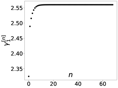
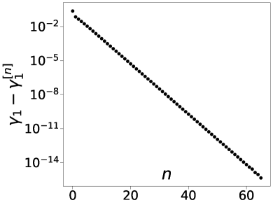
Figure 1: Convergence of the exact Bethe root $\gamma_{1}^{[n]}$ at the $n$-th iteration for world-sheet volume $L=32$ and mode number $\nu=1$. Each dot represents an iteration. On the left the plot with the values of $\gamma_{1}^{[n]}$, while on the right the deviations with respect to the final value. The plot on the right has y-axis in log scale to emphasise the exponential convergence. The starting value is the asymptotic Bethe root, as explained in the previous subsection.

Two excitations.

In the case of two excitations (i.e. $M=1$) we have to fix the worldsheet volume $L$, which is quantised, and then solve the excited-state TBA equations for excitations of mode number $(-\nu,\nu)$, with $\nu=0,1,2,\dots\lfloor L/2\rfloor$. The case of $\nu=0$ is special, because in that case the Bethe roots sit an infinity and the TBA equations are singular, corresponding to a BPS state Baggio:2017kza . All other excitation numbers give well-defined equations which can be readily solved numerically. We find that, after a small number of iterations, the results stabilise, see figure 1. The $Y$ functions also converge and take a form similar to those of figure 2. It is worth stressing that we always find that $Y_{0}(\gamma)>-1$, so that the energy formula and the main TBA equation are well-defined — there are no imaginary terms coming from $\log(1+Y)$; similarly, $Y(\gamma)<1$ so that the convolutions involving $\log(1-Y_{0})$ are also well-defined. This also justifies a posteriori the fact the we interchangeably wrote $N_{0}\log(1-Y)$ or $\log(1-Y)^{N_{0}}$.

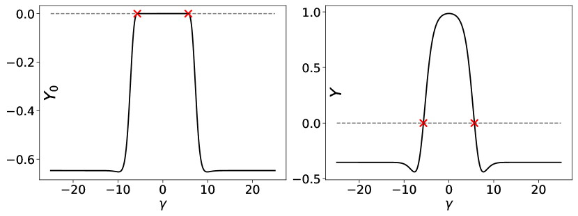
Figure 2: Y functions for a state with $L=256$ and mode number $\nu=1$. On the left $Y_{0}(\gamma)$ and on the right $Y(\gamma)$. The red crosses indicate the positions of the Bethe roots, where both the Y functions are equal to zero and both change sign. $Y_{0}(\gamma)$ takes very small positive values in the interval $[-\gamma_{1},\gamma_{1}]$, since it rapidly converges to zero as $\gamma\to 0$. For $|\gamma|\gg\gamma_{1}$ both Y functions quickly converge to their asymptotic values, see table 1. Even though the plots show only the region $|\gamma|<25$, the cutoff has been set to $\Lambda=40$.

The final result of the evaluation is the leading order correction to the energy of the state, meaning that the energy of a state $|\Psi^{(L,\nu)}\rangle$ identified by $L$ and $\nu$, is

$$\left(\mathbf{L}_{0}+\bar{\mathbf{L}}_{0}\right)|\Psi^{(L,n)}\rangle=H^{(L,\nu)}\,|\Psi^{(L,n)}\rangle,\qquad H^{(L,\nu)}=L+H_{(1)}^{(L,n)}\,h+\mathcal{O}(h^{2})\,,$$ (117)

where $\mathbf{L}_{0}$ and $\bar{\mathbf{L}}_{0}$ are the chiral and antichiral $\mathfrak{sl}(2)$ Cartan elements in the dual CFT, and $h$ is the tension. In other words, we are after $H_{(1)}^{(L,n)}$ which is the leading part of the anomalous dimensions and appears at order $h^{1}$. In figure 3 we plot the energies as a function of $n$ for various values of $L$, namely $L=4,16,32,256$. As it can be expected, the exact value of the energies gets closer to the asymptotic value (i.e., the value predicted by the Bethe-Yang equations) as $L\to\infty$. As it can be seen in figure 4, the deviation from the asymptotic prediction goes like $1/L$. This is expected for a system with gapless excitations in the spectrum. It is also interesting to note that the energy, already for relatively modest values of $L$, such as $L\gtrsim 16$, is well approximated by the black dashed line, corresponding to a free theory with

$$p_{1}=-p_{2}=\frac{2\pi\,\nu}{L}\,,\qquad H_{(1)}^{(L,\nu)}=\sum_{j=1}^{2}\big{|}2\sin(\tfrac{1}{2}p_{j})\big{|}=4\sin\left(\frac{\pi\nu}{L}\right)\,,$$ (118)

with $\nu=0,1,2,\dots\lfloor\frac{L}{2}\rfloor$. That is, with good approximation the system behaves similarly to weakly-interacting massless magnons.

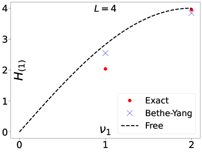
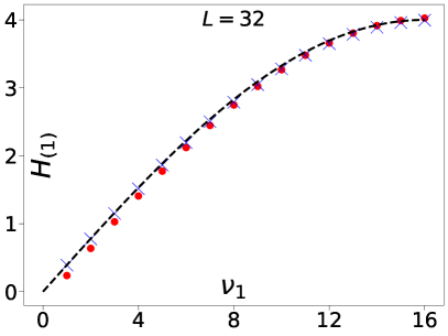
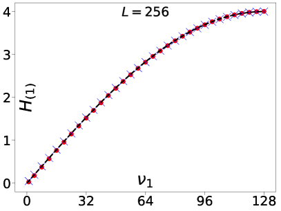
Figure 3: Anomalous dimensions $H_{(1)}$ at order $\order{h}$ in the string tension. The plots are for different values of L, namely $L=4,16,32,256$. In each plot are represented the exact energy from (92), the asymptotic energy from the Bethe-Yang equations, and the energy for a free model, see (118).

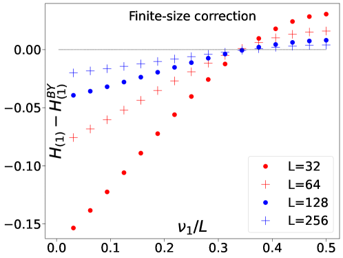
Figure 4: Deviation of the asymptotic energy $H_{(1)}^{BY}$ from the exact energy $H_{(1)}$ for different values of the world-sheet length $L$. The deviation goes like $1/L$.

In figure 4, we see that the difference between the exact solution and the asymptotic one depends on the mode number $\nu_{1}$ and it has a change of sign around $\nu_{1}/L\approx 0.331$ (note however that this value is $L$-dependent). Technically, this can be understood by looking at the exact Bethe equations (91) and the form of the Y-functions in Figure 2. In (91), the corrections to the Bethe-Yang equation are given by the convolutions involving the Y-functions. In particular, one can check from (91) that the exact Bethe root $p_{1}$ is always smaller than the momentum $p_{1}^{\text{BY}}$ of the asymptotic Bethe root (equivalently, $\gamma_{1}>\gamma_{1}^{(\text{BY})}$). First, note that in the region where $\nu/L$ is small, the contribution of the exact roots to the energy is $2|\sin(p/2)|\sim|p|$, and a discrepancy in $p_{1}-p_{1}^{\text{BY}}$ has a big (linear) effect on the energy, which is sufficient to make $H_{(1)}-H_{(1)}^{\text{BY}}<0$. As we increase mode number, both $p_{1}$ and $p_{1}^{\text{BY}}$ get larger with $\nu_{1}/L$, and eventually we get to a regime where $p_{1}\lesssim\pi$. In this region, $|\sin(p/2)|$ is flatter and small deviations in $p_{1}-p_{1}^{\text{BY}}$ affect the energy less and less. Secondly, adding to this effect is the fact that by increasing $\nu/L$, the deviation $|p_{1}-p_{1}^{BY}|$ gets smaller. That deviation is given by the convolutions in (91). As $\nu/L$ gets larger, the Bethe root $\gamma_{1}$ gets closer to zero; when this happens, the integrand is more and more well approximated by an odd function (it is exactly odd for $\gamma_{1}=0$). Thus, the integral gets smaller and smaller. Finally, as we increase the mode, the integral term in (92) becomes more and more important. Looking at figure 2, we see that $Y_{0}(\gamma)$ is approximately constant and negative in a region $|\gamma|\gtrsim\gamma_{1}$. As the mode number grows, $p_{1}$ increases, and $\gamma_{1}$ decreases; hence the contribution of $-\log(1+Y_{0})$ to the energy convolution is larger and larger (and positive). Hence, for $\nu_{1}/L$ sufficiently close to $1/2$, the convolution term dominates, and $H_{(1)}-H_{(1)}^{\text{BY}}>0$. The point where $H_{(1)}-H_{(1)}^{\text{BY}}$ changes sign due to the balancing of these effects does not seem to correspond to a physical mode number. It would be interesting to understand whether this behaviour is fundamentally tied to any underlying physics of the model, or it has no deeper meaning.

Four excitations.

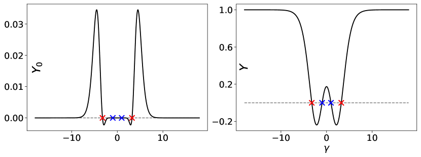
Figure 5: Y functions for a state with $L=16$ and mode numbers $\nu_{1}=1$ and $\nu_{3}=4$. On the left $Y_{0}(\gamma)$ and on the right $Y(\gamma)$. The crosses indicate the positions of the 4 Bethe roots, where both the Y functions are equal to zero and both change sign. The red ones are associated to the modes $(-\nu_{1},\nu_{1})$ and the blue ones to the modes $(-\nu_{3},\nu_{3})$. In $Y_{0}$ the changes of sign due to the bigger Bethe roots (marked by the red crosses) are distinguishable, while the other two (marked by the blue crosses) are not, since again $Y_{0}(\gamma)$ rapidly converges to zero as $\gamma\to 0$. Again, the large $\gamma$ behaviour is the expected one and they quickly converge to their asymptotic values as stated in Table 1. The plots shows the region $\left|\gamma\right|<18$, but again the cutoff has been set to $\Lambda=40$.

Let us now turn to the case of $M=2$, i.e. of four excitations coming in pairs of opposite momentum. Let the mode numbers be $(\nu_{1},-\nu_{1},\nu_{3},-\nu_{3})$ and let us take $\nu_{1}$ and $\nu_{3}$ to be non-negative integers. A special case is that of $\nu_{1}=\nu_{3}$; this is an allowed state, as long as the excitations carry distinct $\mathfrak{su}(2)_{\circ}$ quantum numbers. Let us first discuss the case of generic (different) quantum numbers. In this case, the Y functions go to their vacuum values as $\gamma\to\pm\infty$, see figure 5. It still remains true that $Y_{0}(\gamma)>-1$ and $Y(\gamma)<1$ for any finite $\gamma$ on the real mirror line, so that the TBA equations are well-defined.

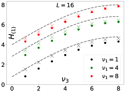
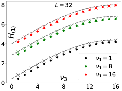
Figure 6: Anomalous dimensions $H_{(1)}$ at order $\order{h}$ in the string tension for $L=16$ and $L=32$. In each plot are represented the energies as function of the mode $\nu_{3}$ for fixed values of $\nu_{1}$. As in the previous energy plots in figure 3, the dots mark the exact energy from (92), the crosses are for the asymptotic energy from the Bethe-Yang equations, and the dashed lines for the energy for a free model, see (118).

For each given $L$, the energy can be computed as a function of $\nu_{3}$ for fixed $\nu_{1}$. Some of the resulting curves are plotted in figure 6 for $L=16$ and $L=32$. Once again, we find that the deviation is relatively small with respect to the asymptotic, or even free, result. Let us now turn to the case of $\nu_{1}=\nu_{3}$. Here, already asymptotically, we see that there are two possible solutions: one with the Bethe roots $\gamma_{1}=\gamma_{3}$ and the other with $\gamma_{1}\neq\gamma_{3}$. Interestingly, it is the solution with $\gamma_{1}\neq\gamma_{3}$ which fits the trajectories of energies in figure 6; the other solution would look like an outlier. It is not clear what would be the interpretation of the configuration with identical roots.

Other values of $N_{0}$.

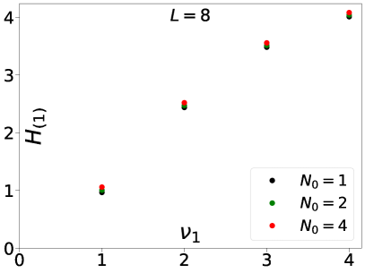
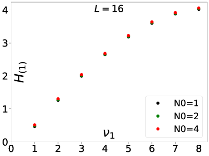
Figure 7: Comparison of the anomalous dimensions of two-particle states ($M=1$) for different values of $N_{0}=1,2,4$. For definiteness, we consider $L=8$ and $L=16$. For states with larger $L$, the difference becomes even smaller.

In Frolov:2023wji , the mirror TBA for a twisted vacuum was discussed, and the ground state energies were computed. This is done by taking the volume $L\to\infty$ while keeping the tension fixed. The computation can be then formally compared with a semiclassical one, where $L\to\infty$ and $h\to\infty$ with $\mathcal{J}=L/h$ fixed. In both approaches, it is easy to keep track of the contribution of gapless and gapped (mirror) particles. Indeed, at large $\mathcal{J}$ the gapless particles contribute at order $1/\mathcal{J}$ while the gapped ones at order $e^{-\mathcal{J}}/\sqrt{\mathcal{J}}$. For the gapped particles, the precise form of the contribution seems to match with the semiclassical prediction (up to identifying the twist in a specific way). For gapless ones, it does not, unless one assumes $N_{0}=1$ in the mirror TBA — in which case it does. While a discrepancy might be explained by the different ways in which the limit is taken in the mirror TBA and in the semiclassical computation, it is highly suggestive that the results do match as far as the massive contribution goes (and they do match in $\text{AdS}_{5}\times\text{S}^{5}$ Frolov:2009in ; Frolov:2023wji ). While the physical interpretation of putting $N_{0}=1$ is unclear, it is worth exploring the effect of such a choice (or on setting $N_{0}\neq 2$ in general) on the spectrum. What we find is that nothing special seems to happen. Indeed, the numerical value of the energies changes in a mild way as we change $N_{0}$, see figure 7. Unfortunately, this does not suggest how to resolve the puzzle of Frolov:2023wji , as no choice of $N_{0}$ appears pathological or particularly “nice”. The only way to obtain a sure answer would be a direct quantitative comparison with predictions either from string theory, which would necessitate extending this analysis to the semiclassical regime.

8 Conclusions and outlook

We derived the weak-tension expressions for the mirror TBA for pure-RR $\text{AdS}_{3}\times\text{S}^{3}\times\text{T}^{4}$ with massless particle excitations and solved the corresponding equations numerically. We find that the leading order correction to the energy comes from the massless sector at order $\mathcal{O}(T)$ in the tension $T\ll 1$, while the massive sector is suppressed to $\mathcal{O}(T^{2L})$, where $L$ is the R-charge of a reference vacuum (i.e., a reference BPS state). This is strikingly different from $\text{AdS}_{5}\times\text{S}^{5}$, where there is no massless sector at all. It was natural to expect that the dynamics at $\mathcal{O}(T)$ should be substantially simpler than the full worldsheet dynamics at arbitrary tension. What was unclear was whether such the weak-tension physics could be understood as a nearest-neighbour spin chain (like in $\text{AdS}_{5}\times\text{S}^{5}$) or as a symmetric orbifold CFT of a free model (like in the case of the tensionless limit of pure-NSNS backgrounds). By solving numerically the equations we determine that it is neither. The fact that a nearest-neighbour description would be too simple a dynamics was already strongly implied by the presence of gapless (i.e., long range) excitations.

At weak tension, the model is given by a system of TBA equations of difference-form, with a nonrelativistic energy and momentum. From the numerical solution of the spectrum, we find that it represents a system of weakly-interacting massless magnons, with energy $\mathcal{E}(p)\sim|\sin(p/2)|$. The deviation of the exact energies from the asymptotic model is of order $1/L$ — as it is the of deviation of the asymptotic result from the free one. It would be interesting to see if one may reverse-engineer a scattering phase $\varphi_{\text{eff}}$ so that the exact energies are given by

$$e^{ip_{j}L}\prod_{k\neq j}e^{i\varphi_{\text{eff}}(p_{j},p_{k})}=1,\qquad\mathcal{E}=\sum_{j}\mathcal{E}(p_{j})\,.$$ (119)

Of course this is generally impossible for a system of TBA equations, but perhaps at leading order the dynamics of the model is so simple to allow for such a simplification. A brief exploration of this idea however did not result in a perfect match of the energies when using a few known scattering phases. It is also interesting to explore whether this spectrum may correspond to any known quantum-mechanical integrable model with long-range interactions.

We have also explored the question of how many species of massless particles should be included in the TBA. From perturbation theory we expect to have $N_{0}=2$ types of excitations, but in recent work it was observed Frolov:2023wji that setting $N_{0}=1$ seem to better account for the energy of a twisted ground state. We find that, for excited states at small tension, any value of $N_{0}$ yields an apparently reasonable solution, and in fact the deviations between $N_{0}=1$, $N_{0}=2$, and (for the sake of generality) $N_{0}=4$ are numerically small. Hence, this does not seem to resolve the confusion on this point. One way to resolve this puzzle might be to derive the mirror TBA equations for the ${\rm AdS}_{3}\times{\rm S}^{3}\times{\rm S}^{3}\times{\rm S}^{1}$ background Tong:2014yna ; Borsato:2015mma , and study their $\text{T}^{4}$ limit.

Aside from the TBA, there is another proposal for a system of equations describing the spectrum: the quantum spectral curve Ekhammar:2021pys ; Cavaglia:2021eqr ; Cavaglia:2022xld . It would be interesting to use those equations to extract the small-tension spectrum and compare with our results. Unfortunately, it is currently unclear if and how the QSC equations account for states including massless excitations, which are the ones with the largest anomalous dimension in this regime. Hence, our results cannot be compared with that framework, at least until it is possible to adapt the QSC to describe states involving massless excitations.

Acknowledgements

We thank Sergey Frolov, Alessandro Torrielli, Arkady Tseytlin, and Linus Wulff for useful related discussions. We are particularly grateful to Stefano Scopa for discussions and help with the Python code for the numerical solution of the TBA equations. DlP acknowledges support from the Stiftung der Deutschen Wirtschaft. The work of RS is supported by NSFC grant no. 12050410255. AS thanks the participants of the workshop “Integrability in Low-Supersymmetry Theories” in Filicudi, Italy, for a stimulating environment where part of this work was carried out. AS acknowledges support from the European Union – NextGenerationEU, and from the program STARS@UNIPD, under project “Exact-Holography – A new exact approach to holography: harnessing the power of string theory, conformal field theory, and integrable models.”

Appendix A Notation

Here we summarise our notation, various S-matrix elements and kernels.

A.1 Rapidity variables

We will use three types of variables to express the S-matrices: $x$-variable, $u$-rapidity and $\gamma$-variable. When working with the $u$-rapidity, we introduce the notation$f^{\pm}(u)\equiv f(u\pm i|m|/h)$, where the value of $|m|=Q=\bar{Q}$ is the mass of the particle.

Mirror momentum-carrying particles.

The map from Zhukovsky variables to rapidity variables in the mirror region is

$$x^{+}(\gamma^{+})=\frac{1+e^{\gamma^{+}}}{1-e^{\gamma^{+}}}\,,\qquad x^{-}(\gamma^{-})=\frac{1-e^{\gamma^{-}}}{1+e^{\gamma^{-}}}\,,\qquad x(\gamma)=-\tanh\frac{\gamma}{2}\,.$$ (120)

Here $x^{\pm}$ and $\gamma^{\pm}$ refer to massive particles, and for real mirror particles obey the reality constraint

$$(x^{\pm})^{*}=\frac{1}{x^{\mp}}\,,\qquad(\gamma^{\pm})^{*}=\gamma^{\mp}\,,$$ (121)

while $\gamma$ is real for real-momentum mirror particles. The same formulae can be found by using the $u$-paramatrisation

$$u(\gamma)=-2\coth\gamma\,,\qquad\gamma(u)=\frac{1}{2}\log\frac{2-u}{2+u}+\frac{i\pi}{2}$$ (122)

and recalling that

$$x(u)=\frac{1}{2}\left(u-i\sqrt{4-u^{2}}\right)\,,$$ (123)

which confirms that indeed for $\gamma$ just above the real line

$$x(\gamma):=x(u(\gamma+i0))\,.$$ (124)

Vice versa we have

$$\gamma(x)=-2\,\text{atanh}\,x\,,\qquad\gamma(u):=\gamma(x(u))\,.$$ (125)

We can use $\gamma(u)$ to define

$$\gamma^{+}(u) =\gamma(u+\tfrac{i}{h}|m|)-i\pi, \quad x^{+}(u) =x^{+}(\gamma^{+}(u)),$$ (126)

$$\gamma^{-}(u) =\gamma(u-\tfrac{i}{h}|m|), \quad x^{-}(u) =x^{-}(\gamma^{-}(u)),$$

which is compatible with our mirror reality. The relation between $\gamma^{\pm}$ and $x^{\pm}$ is then

$$\gamma^{\pm}(x^{\pm})=\log\left(i\frac{x^{\pm}-1}{x^{\pm}+1}\right)\mp i\frac{\pi}{2}\,.$$ (127)

Finally we recall that both $\gamma^{\pm}$ and $x^{\pm}$ are not sets of independent variables, because

$$\frac{h}{i}\left(\coth\gamma^{-}-\coth\gamma^{+}\right)=\frac{h}{2i}\left(x^{+}+\frac{1}{x^{+}}-x^{+}-\frac{1}{x^{+}}\right)=|m|\,.$$ (128)

Mirror branch cuts and massless physical region.

It is important to note that massless mirror particles, are defined for

$$x\in(-1,+1),\quad\gamma\in(-\infty+i0,+\infty+i0)\,,\quad u\in(-\infty+i0,-2+i0)\cup(+2+i0,+\infty+i0)\,.$$ (129)

In other words, the region in the $u$-plane is just above the long cut. The mirror momentum and energy for massless particles are given by

$$\tilde{p}_{0}(\gamma)=-\frac{2h}{\sinh\gamma}\,,\qquad\tilde{\mathcal{E}}_{0}(\gamma)=-\log\left(\frac{1-e^{\gamma}}{1+e^{\gamma}}\right)^{2}\,.$$ (130)

Note that the second formula is not analytic along the imaginary axis of the $\gamma$-plane (much like $\log z^{2}$). It is sometimes useful to treat separately the positive and negative momentum regions. For this purpose note that $\tilde{p}_{0}>0$ corresponds to

$$\tilde{p}_{0}>0\,:\qquad x\in(0,+1),\qquad\gamma\in(-\infty+i0,0+i0)\,,\qquad u\in(+2+i0,+\infty+i0)\,.$$ (131)

String momentum-carrying particles.

The kinematics of the string region can be obtained by analytic continuation but for us it is most useful to use distinct $\gamma$-parametrisation. We indicate string-kinematics expressions by a subscript “$s$”. We have

$$x^{+}_{s}(\gamma^{+}_{s})=\frac{i-e^{\gamma^{+}_{s}}}{i+e^{\gamma^{+}_{s}}}\,,\qquad x^{-}_{s}(\gamma^{+}_{s})=\frac{i+e^{\gamma^{-}_{s}}}{i-e^{\gamma^{-}_{s}}}\,,\qquad x_{s}(\gamma_{s})=\frac{i-e^{\gamma_{s}}}{i+e^{\gamma_{s}}}\,.$$ (132)

For massive particles the reality condition is

$$(x^{+}_{s})^{*}=x^{-}_{s}\,,\qquad(\gamma^{+}_{s})^{*}=\gamma^{-}_{s}\,,$$ (133)

whereas $\gamma_{s}$ is once again real for real (string) particles. In terms of the $u$-rapidity we have

$$u=-2\tanh\gamma_{s}\,,\qquad\gamma_{s}(u)=\frac{1}{2}\log\frac{u-2}{u+2}-i\frac{\pi}{2}\,.$$ (134)

In contrast to (122), now the cuts on the $u$-plane are short (they run from $-2$ to $+2$), as it is the case in the formula for

$$x_{s}(u)=\frac{u}{2}\left(1+\sqrt{1-\frac{4}{u^{2}}}\right)\,.$$ (135)

Indeed it can be checked that

$$x_{s}(\gamma_{s}):=x_{s}(u(\gamma_{s}-i0))\,,$$ (136)

with $\gamma_{s}$ just below the real line so that $u$ is just above the short cut and $x_{s}$ is on the upper half-circle. We can also define

$$\gamma_{s}^{-}(u)=\gamma_{s}(u-\tfrac{i}{h}|m|)-i\pi\,,\qquad\gamma_{s}^{+}(u)=\gamma_{s}(u+\tfrac{i}{h}|m|).$$ (137)

In terms of $x^{\pm}$ we have

$$\gamma^{\pm}_{s}(u)=\log\left(\mp i\frac{x^{\pm}-1}{x^{\pm}+1}\right)\,.$$ (138)

Finally, we have the constraint

$$\frac{h}{i}\left(\tanh\gamma^{-}_{s}-\tanh\gamma^{+}_{s})\right)=\frac{h}{2i}\left(x^{+}_{s}+\frac{1}{x^{+}_{s}}-x^{+}_{s}-\frac{1}{x^{+}_{s}}\right)=|m|\,.$$ (139)

String branch cuts and massless physical region.

Also in this region, string massless particles live on the $u$-plane branch cut, which is now short. Real-momentum particles satisfy

$$x_{s}\in\mathbb{S}^{1}_{+},\quad\gamma_{s}\in(-\infty-i0,+\infty-i0)\,,\quad u\in(-2+i0,+2+i0)\,,$$ (140)

where $\mathbb{S}^{1}_{+}$ is upper-half circle. The string energy and momentum are

$$\mathcal{E}_{0}(\gamma_{s})=\frac{2h}{\cosh\gamma_{s}}\,,\qquad p_{0}(\gamma_{s})=-i\log\left(\frac{i-e^{\gamma_{s}}}{i+e^{\gamma_{s}}}\right)^{2},$$ (141)

where the latter is not analytic across the imaginary axis.

Auxiliary (mirror) particles.

Finally, we have the auxiliary $y^{+}$ and $y^{-}$ particles. In the mirror region, they lie on the upper and lower half-circle respectively. As such, we can parametrise them using the same variables as massless string particles.

• $y^{+}$ particles

  $$y(u)=x_{s}(u+i0)=x_{s}(u(\gamma_{s}-i0)),\qquad-2\leq u\leq\,,\quad\gamma_{s}\in\mathbb{R}\,,$$ (142)

• $y^{-}$ particles

  $$y(u)=\frac{1}{x_{s}(u+i0)}=\frac{1}{x_{s}(u(\gamma_{s}-i0))},\qquad-2<u<2\,,\quad\gamma_{s}\in\mathbb{R}\,.$$ (143)

Note that $x_{s}(u+i0)=1/x(u)$ for $-2\leq u\leq 2$.

Shift-identity.

While we will generally think of the string and mirror variables $\gamma$ and $\gamma_{s}$ as independent, there is a simple relation that allows us to go from one to the other, namely

$$\gamma_{s}=\gamma-\frac{i\pi}{2}\,.$$ (144)

This can be useful in finding various kernels and S matrices. In particular, note that

$$i\,\mathcal{E}_{0}(\gamma-\tfrac{i\pi}{2})=\tilde{p}_{0}(\gamma)\,,\qquad i\,p_{0}(\gamma-\tfrac{i\pi}{2})=\tilde{\mathcal{E}}_{0}(\gamma)\,.$$ (145)

S-matrices.

In view of the above, it is natural to define the following notation. Given the S-matrix $S(x,x^{\prime})$ which depends on two massive variables, we rewrite it in terms of the $u$- and $\gamma$-variable as

$$S(u,u^{\prime})=S^{AB}(x(u),x(u^{\prime})),\qquad S(\gamma,\gamma^{\prime})=S^{AB}(x(\gamma),x(\gamma^{\prime})).$$ (146)

Here the $u$ and $\gamma$ variables are in the mirror physical region (129). For massive particles we always use the standard $u$-parametrisation to define the S matrix and kernels, that is e.g.

$$S^{AB}(u,u^{\prime})=S^{AB}(x^{\pm}(u),x^{\pm}(u^{\prime})).$$ (147)

For the scattering of auxiliary particles in the mirror region we use

$$S^{Ay}(u,u^{\prime})=S^{AB}(x(u),x_{s}(u^{\prime}+i0)),\qquad S^{Ay}(\gamma,\gamma^{\prime})=S^{AB}(x(\gamma),x_{s}(\gamma^{\prime}-i0))$$ (148)

for both $y^{+}$ and $y^{-}$ particles, as exemplified in (59). The mirror auxiliary particle lives is parametrised in terms of the physical region as the massless string particle, that is (140).

A.2 Kernels in $\gamma$-rapidity parametrisation

We define the kernels as

$$K^{AB}(u,u^{\prime})=\frac{1}{2\pi i}\frac{\text{d}}{\text{d}u}\log S^{AB}(u,u^{\prime})\,,\qquad\mathcal{K}^{AB}(\gamma,\gamma^{\prime})=\frac{1}{2\pi i}\frac{\text{d}}{\text{d}\gamma}\log S^{AB}(\gamma,\gamma^{\prime})\,,$$ (149)

so that

$$K^{AB}(u,u^{\prime})=\frac{\text{d}\gamma}{\text{d}u}\,\mathcal{K}^{AB}(\gamma(u),\gamma(u^{\prime}))\,.$$ (150)

With these kernels, define the left-convolution

$$(f*\mathcal{K})(\gamma^{\prime})=\int\limits_{-\infty}^{+\infty}\text{d}\gamma\,f(\gamma)\,\mathcal{K}(\gamma,\gamma^{\prime}),,$$ (151)

which we will use to rewrite the TBA equations. When a kernel is of difference type, this means

$$(f*\mathcal{K})(\gamma^{\prime})=\int\limits_{-\infty}^{+\infty}\text{d}\gamma f(\gamma)\,\mathcal{K}(\gamma-\gamma^{\prime})\,.$$ (152)

We also note that the sign may change,

$$\left(f\,\hat{\star}\,K^{yA}\right)(v) =\int\limits_{-2}^{+2}\text{d}u\,f(u)\,K^{yA}(u,v)$$ (153)

$$=-\int\limits_{-\infty}^{+\infty}\text{d}\gamma\,f(u(\gamma))\,\frac{\text{d}u}{\text{d}\gamma}\,K^{yA}(u(\gamma),v(\gamma^{\prime}))=-\left(f*\mathcal{K}^{yA}\right)(\gamma^{\prime})\,.$$

This is because $x_{s}(\gamma)$ parameterises the upper half plane counter-clockwise, while $x_{s}(u+i0)$ parameterises it clockwise. This is not the case for the integration over $(-\infty,-2)\cup(2,\infty)$, where $(\text{d}\gamma/\text{d}u)$ remains positive. We have schematically

$$f\,\hat{\star}\,g\to-f*g,\qquad f\,\check{\star}\,g\to+f*g.$$ (154)

A.3 List of S matrices

We basically use the same notation as Appendix B in Frolov:2021bwp . Whenever the $u$-rapidity lies on the branch cut, we always take the $u+i0$ prescription.

The standard bound state S matrix is

$$S^{QQ^{\prime}}(u-u^{\prime})=S^{Q+Q^{\prime}}(u-u^{\prime})S^{Q-Q^{\prime}}(u-u^{\prime})\prod_{j=1}^{Q^{\prime}-1}S^{Q-Q^{\prime}+2j}(u-u^{\prime}),$$ (155)

where $S^{Q}$ is the rational S-matrix

$$S^{Q}(u,u^{\prime})=\frac{u-u^{\prime}-\frac{iQ}{h}}{u-u^{\prime}+\frac{iQ}{h}}$$ (156)

Left-anything scattering.

$$S_{\textit{sl}}^{Q_{a}Q_{b}}(u_{a},u_{b}) =S^{Q_{a}Q_{b}}(u_{a}-u_{b})^{-1}(\Sigma_{ab}^{Q_{a}Q_{b}})^{-2}\,,$$ (157)

$$\tilde{S}_{\textit{sl}}^{Q_{a}\bar{Q}_{b}}(u_{a},u_{b}) =e^{ip_{a}}\frac{1-\frac{1}{x_{a}^{+}x_{b}^{+}}}{1-\frac{1}{x_{a}^{-}x_{b}^{-}}}\frac{1-\frac{1}{x_{a}^{+}x_{b}^{-}}}{1-\frac{1}{x_{a}^{-}x_{b}^{+}}}(\tilde{\Sigma}_{ab}^{Q_{a}\bar{Q}_{b}})^{-2}\,,$$ (158)

$$S^{Q_{a}0}(u_{a},x_{j}) =ie^{-\frac{i}{2}p_{a}}\frac{x_{a}^{+}x_{j}-1}{x_{a}^{-}-x_{j}}\frac{(\Sigma_{{\text{\tiny BES}}}^{Q_{a}0}(x_{a}^{\pm},x_{j}))^{-2}}{\varPhi(\gamma_{aj}^{+\circ})\varPhi(\gamma_{aj}^{-\circ})}\,,$$ (159)

$$S_{+}^{Q_{a}y}(u,v) =e^{\tfrac{i}{2}p_{a}}\,\frac{x^{-}(u_{a})-x(v)}{x^{+}(u_{a})-x(v)}\,,$$ (160)

$$S_{-}^{Q_{a}y}(u,v) =e^{\tfrac{i}{2}p_{a}}\,\frac{x^{-}(u_{a})-\frac{1}{x(v)}}{x^{+}(u_{a})-\frac{1}{x(v)}}\,,$$ (161)

where $\varPhi=e^{\varphi}$ is the sine-Gordon factor (183), and $\gamma^{\pm\circ}_{aj}=\gamma^{\pm}_{a}-\gamma_{j}$ . The improved BES factors such as $\Sigma^{Q_{a}Q_{b}}$ and $\Sigma_{{\text{\tiny BES}}}^{Q_{a}0}$ will be discussed in Appendix D.1.

Right-anything scattering.

$$S_{\textit{su}}^{\bar{Q}_{a}\bar{Q}_{b}}(u_{a},u_{b}) =e^{ip_{a}}e^{-ip_{b}}\left(\frac{x_{a}^{+}-x_{b}^{-}}{x_{a}^{-}-x_{b}^{+}}\right)^{-2}S^{\bar{Q}_{a}\bar{Q}_{b}}(u_{a}-u_{b})^{-1}(\Sigma_{ab}^{\bar{Q}_{a}\bar{Q}_{b}})^{-2}\,,$$ (162)

$$\tilde{S}_{\textit{su}}^{\bar{Q}_{a}Q_{b}}(u_{a},u_{b}) =e^{-ip_{b}}\frac{1-\frac{1}{x_{a}^{-}x_{b}^{-}}}{1-\frac{1}{x_{a}^{+}x_{b}^{+}}}\frac{1-\frac{1}{x_{a}^{+}x_{b}^{-}}}{1-\frac{1}{x_{a}^{-}x_{b}^{+}}}(\tilde{\Sigma}_{ab}^{\bar{Q}_{a}Q_{b}}(u_{a},u_{b}))^{-2}\,,$$ (163)

$$\tilde{S}^{\bar{Q}_{a}0}(u_{a},x_{j}) =ie^{+\frac{i}{2}p_{a}}\frac{x_{a}^{-}-x_{j}}{x_{a}^{+}x_{j}-1}\frac{(\Sigma_{{\text{\tiny BES}}}^{\bar{Q}_{a}0}(x_{a}^{\pm},x_{j}))^{-2}}{\varPhi(\gamma_{aj}^{+\circ})\varPhi(\gamma_{aj}^{-\circ})}\,.$$ (164)

Massless-anything scattering.

$$S^{00}(u_{j},u_{k}) =a(\gamma_{jk})\varPhi(\gamma_{jk})^{2}(\Sigma_{{\text{\tiny BES}}}^{00}(x_{j},x_{k}))^{-2}\,,$$ (165)

$$S^{0Q_{b}}(x_{j},u_{b}) =\frac{1}{S^{Q_{b}0}(u_{b},x_{j})}\,,$$ (166)

$$\tilde{S}^{0\bar{Q}_{b}}(x_{j},u_{b}) =\frac{1}{\tilde{S}^{\bar{Q}_{b}0}(u_{b},x_{j})}\,,$$ (167)

$$S^{0y}(u,v) =\frac{1}{\sqrt{x(u+i0)^{2}}}\frac{x(u+i0)-x_{s}(v+i0)}{\frac{1}{x(u+i0)}-x_{s}(v+i0)}\,.$$ (168)

Auxiliary-anything scattering.

$$S^{yQ}_{-}(v,u_{j}) =e^{+\tfrac{i}{2}p_{j}}\frac{\frac{1}{x(v)}-x^{-}(u_{j})}{\frac{1}{x(v)}-x^{+}(u_{j})}=S^{Qy}_{-}(u_{j},v),$$ (169)

$$S^{yQ}_{+}(v,u_{j}) =e^{-\tfrac{i}{2}p_{j}}\frac{x(v)-x^{+}(u_{j})}{x(v)-x^{-}(u_{j})}=\frac{1}{S^{Qy}_{+}(u_{j},v)}\,,$$ (170)

$$S^{y0}(v,u_{j}) =\frac{1}{\sqrt{x(u_{j}+i0)^{2}}}\,\frac{x(v)-x(u_{j}+i0)}{x(v)-\frac{1}{x(u_{j}+i0)}}=\frac{1}{S^{0y}(u_{j},v)}\,.$$ (171)

These $S^{yQ}_{\mp}(v,u)$ are identical to $S^{yQ}_{\pm}(v,u)$ in Arutyunov:2009ax , and the corresponding kernels are positive in the mirror-mirror region.

Analytic continuation.

The symbol $S^{AB}(u_{1},u_{2})$ usually denotes an S-matrix in the mirror-mirror region. When one of the rapidities is analytically continued to the string region, say $u_{1}$, they are denoted interchangeably by

$$S^{AB}(u_{*1},u_{2}),\quad S^{A_{*}B}(u_{1},u_{2})\quad{\rm or}\quad S^{A_{*}B}(u_{*1},u_{2}).$$ (172)

When the S-matrix is written in the $\gamma$-parametrisation, $S^{AB}(\gamma_{1},\gamma_{2})$, then we perform the analytic continuation as explained in Frolov:2021fmj . For massless particles, the string region is $i\pi/2$ above the mirror region. To describe the rapidity in the string region, we use the notation $\gamma-\frac{i\pi}{2}\equiv\gamma_{*}\in\mathbb{R}$ as in (144). For massive particles, the string region is $i\pi/2$ below the mirror region.

Cauchy kernel.

$$s(\gamma)=\frac{1}{2\pi i}\,\frac{\text{d}}{\text{d}\gamma}\log S(\gamma)=\frac{1}{2\pi\cosh{\gamma}}\,,\qquad S(\gamma)=-i\tanh\left(\frac{\gamma}{2}-\frac{i\pi}{4}\right).$$ (173)

The multiplicative normalisaton of $S(\gamma)$ has been chosen so that

$$S(0)=-1\,.$$ (174)

The “analytically continued” (i.e. shifted) kernel is

$$s_{*}(\gamma)=s(\gamma+\tfrac{i\pi}{2})=\frac{1}{2\pi i\,\sinh\gamma}\,,\qquad S_{*}(\gamma)=S(\gamma+\tfrac{i\pi}{2})=-i\tanh\frac{\gamma}{2}\,.$$ (175)

The (right-)inverse Cauchy kernel is the following difference operator,

$$(f*s^{-1})(\gamma)=f(\gamma+\frac{i\pi}{2}-i0)+f(\gamma-\frac{i\pi}{2}+i0).$$ (176)

Cauchy kernel satisfies

$$(1*s)(\gamma)=\frac{1}{2},\qquad(s*s)(\gamma)=\frac{\gamma}{2\pi^{2}\,\sinh(\gamma)}=\mathcal{K}_{\text{SG}}(\gamma)\,,$$ (177)

where $\mathcal{K}_{\text{SG}}(\gamma)$ is the sine-Gordon kernel,

$$\mathcal{K}_{\text{SG}}(\gamma)=\frac{1}{2\pi i}\,\frac{\text{d}}{\text{d}\gamma}\log\varPhi(\gamma)=\frac{1}{2\pi i}\,\frac{\text{d}}{\text{d}\gamma}\varphi(\gamma)\,,$$ (178)

as defined in (183). Furthermore we have that

$$\int\limits_{-\infty}^{+\infty}\text{d}\gamma^{\prime}\,\log\left(-S(\gamma-\gamma^{\prime})\right)s(\gamma^{\prime}-\gamma^{\prime\prime})=\varphi(\gamma-\gamma^{\prime\prime})\,.$$ (179)

A.4 Massive dressing factors

The massive dressing factors in the mirror-mirror kinematics, with $Q,Q^{\prime}=1,2,\dots$ are given in appendix C of Frolov:2021bwp and read

$$(\Sigma_{12}^{QQ^{\prime}})^{-2} =-\frac{\sinh{\frac{\gamma_{12}^{-+}}{2}}}{\sinh{\frac{\gamma_{12}^{+-}}{2}}}e^{\varphi^{\bullet\bullet}(\gamma_{1}^{\pm},\gamma_{2}^{\pm})}(\Sigma_{{\text{\tiny BES}}}^{QQ^{\prime}}(x_{1}^{\pm},x_{2}^{\pm}))^{-2}\,,$$ (180)

$$(\tilde{\Sigma}_{12}^{QQ^{\prime}})^{-2} =+\frac{\cosh{\frac{\gamma_{12}^{+-}}{2}}}{\cosh{\frac{\gamma_{12}^{-+}}{2}}}e^{\tilde{\varphi}^{\bullet\bullet}(\gamma_{1}^{\pm},\gamma_{2}^{\pm})}(\Sigma_{{\text{\tiny BES}}}^{QQ^{\prime}}(x_{1}^{\pm},x_{2}^{\pm}))^{-2}\,.$$

We define the corresponding kernels by

$$K_{\Sigma}^{Q_{1}Q_{2}}(u_{1},u_{2}) =\frac{1}{2\pi i}\frac{\partial}{\partial u_{1}}\log\Sigma_{12}^{Q_{1}Q_{2}}(x_{1}^{\pm},x_{2}^{\pm}),$$ (181)

$$\tilde{K}_{\Sigma}^{Q_{1}Q_{2}}(u_{1},u_{2}) =\frac{1}{2\pi i}\frac{\partial}{\partial u_{1}}\log\tilde{\Sigma}_{12}^{Q_{1}Q_{2}}(x_{1}^{\pm},x_{2}^{\pm}).$$

The phases $\varphi^{\bullet\bullet}$ and $\tilde{\varphi}^{\bullet\bullet}$ are given by eq. (5.6) in Frolov:2021fmj and can be expressed as

$$e^{\varphi^{\bullet\bullet}(\gamma_{1}^{\pm},\gamma_{2}^{\pm})} =\exp\Bigl(\varphi_{+}(\gamma_{12}^{--})+\varphi_{+}(\gamma_{12}^{++})+\varphi_{-}(\gamma_{12}^{-+})+\varphi_{-}(\gamma_{12}^{+-})\Bigr{missing}),$$ (182)

$$e^{\tilde{\varphi}^{\bullet\bullet}(\gamma_{1}^{\pm},\gamma_{2}^{\pm})} =\exp\Bigl(\varphi_{-}(\gamma_{12}^{--})+\varphi_{-}(\gamma_{12}^{++})+\varphi_{+}(\gamma_{12}^{-+})+\varphi_{+}(\gamma_{12}^{+-})\Bigr{missing}),$$

where the functions

$$\varphi_{-}(\gamma) =+\frac{i}{\pi}\text{Li}_{2}\left(+e^{\gamma}\right)-\frac{i}{4\pi}\gamma^{2}+\frac{i}{\pi}\gamma\,\log\left(1-e^{\gamma}\right)-\frac{i\pi}{6}\,,$$ (183)

$$\varphi_{+}(\gamma) =-\frac{i}{\pi}\text{Li}_{2}\left(-e^{\gamma}\right)+\frac{i}{4\pi}\gamma^{2}-\frac{i}{\pi}\gamma\,\log\left(1+e^{\gamma}\right)-\frac{i\pi}{12}\,,$$

were introduced. These formulae are valid when $\gamma$ is in the strip between zero and $i\pi$. We will also use

$$\varphi(\gamma) \equiv\varphi_{+}(\gamma)+\varphi_{-}(\gamma)$$ (184)

$$=\frac{i}{\pi}\text{Li}_{2}(-e^{-\gamma})-\frac{i}{\pi}\text{Li}_{2}(e^{-\gamma})+\frac{i\gamma}{\pi}\log(1-e^{-\gamma})-\frac{i\gamma}{\pi}\log(1+e^{-\gamma})+\frac{i\pi}{4}\,,$$

$$\widehat{\varphi}(\gamma) \equiv\varphi_{+}(\gamma)-\varphi_{-}(\gamma)$$

$$=\frac{i}{2\pi}\text{Li}_{2}\left(e^{-2\gamma}\right)-\frac{i}{2\pi}\gamma^{2}-\frac{i}{\pi}\log\left(1-e^{-2\gamma}\right)-\frac{i\pi}{12}\,,$$

noting that the $\varphi(\gamma)$ is the Sine-Gordon dressing factor. We find crossing-like relations

$$e^{\varphi_{+}(\gamma)+\varphi_{-}(\gamma+\pi i)} =\frac{1}{2\cosh\tfrac{\gamma}{2}}\,, \qquad e^{\varphi_{+}(\gamma)+\varphi_{-}(\gamma-\pi i)} =2\cosh\frac{\gamma}{2}\,,$$ (185)

$$e^{\varphi_{-}(\gamma)+\varphi_{+}(\gamma+\pi i)} =2i\sinh\frac{\gamma}{2}\,,\qquad \qquad e^{\varphi_{-}(\gamma)+\varphi_{+}(\gamma-\pi i)} =\frac{i}{2\sinh\tfrac{\gamma}{2}}\,,$$

$$e^{\varphi_{+}(\gamma)-\varphi_{+}(\gamma+2\pi i)} =\frac{-1}{4\cosh^{2}\tfrac{\gamma}{2}}\,, \qquad e^{\varphi_{-}(\gamma)-\varphi_{-}(\gamma-2\pi i)} =-4\sinh^{2}\frac{\gamma}{2}\,.$$

The improved BES factor for $QQ^{\prime}$ particles is the same as in Arutyunov:2009kf ,

$$\frac{1}{i}\log\Sigma^{QQ^{\prime}}_{\text{\tiny BES}}(x_{1}^{\pm},x_{2}^{\pm})=\Phi(x_{1}^{+},x_{2}^{+})-\Phi(x_{1}^{+},x_{2}^{-})-\Phi(x_{1}^{-},x_{2}^{+})+\Phi(x_{1}^{-},x_{2}^{-})$$ (186)

$$\qquad\qquad-\frac{1}{2}\left(\Psi(x_{1}^{+},x_{2}^{+})+\Psi(x_{1}^{-},x_{2}^{+})-\Psi(x_{1}^{+},x_{2}^{-})-\Psi(x_{1}^{-},x_{2}^{-})\right)$$

$$\qquad\qquad+\frac{1}{2}\left(\Psi(x_{2}^{+},x_{1}^{+})+\Psi(x_{2}^{-},x_{1}^{+})-\Psi(x_{2}^{+},x_{1}^{-})-\Psi(x_{2}^{-},x_{1}^{-})\right)$$

$$\qquad\qquad+\frac{1}{i}\log\frac{i^{Q}\,\Gamma\big{[}Q^{\prime}-\frac{i}{2}h\big{(}x_{1}^{+}+\frac{1}{x_{1}^{+}}-x_{2}^{+}-\frac{1}{x_{2}^{+}}\big{)}\big{]}}{i^{Q^{\prime}}\Gamma\big{[}Q+\frac{i}{2}h\big{(}x_{1}^{+}+\frac{1}{x_{1}^{+}}-x_{2}^{+}-\frac{1}{x_{2}^{+}}\big{)}\big{]}}\frac{1-\frac{1}{x_{1}^{+}x_{2}^{-}}}{1-\frac{1}{x_{1}^{-}x_{2}^{+}}}\sqrt{\frac{x_{1}^{+}x_{2}^{-}}{x_{1}^{-}x_{2}^{+}}}\,,$$

where $\Phi(x_{1},x_{2})$ and $\Psi(x_{1},x_{2})$ will be given in Appendix D.

A.5 Mixed-mass dressing factors

To define mixed-mass scattering elements in the mirror TBA it is sufficient to use the Sine-Gordon dressing factor $\varPhi$,

$$\varPhi(\gamma)=e^{\varphi(\gamma)}\,,$$ (187)

given in the previous subsection, as well as an appropriate generalisation of the BES phase Frolov:2021fmj . We can obtain the (improved) mixed-mass BES dressing factor from (186) by setting $Q=0$ or $Q^{\prime}=0$ as needed.

We will also need to consider the string-mirror and mirror-string kinematics, when the massless excitation is on the string region. By setting $Q=0$, we find the Zukovsky variable $x$ of massless particles in the string region sitting on the upper-half circle. There is an apparent problem, however, with the BES phase: the massless particle sits on the integration contour, leading to a potential single pole. Consider for definiteness $\Sigma_{\sigma_{\text{\tiny BES}}}^{0Q}(x,y^{\pm})$. Potential issues arise from the integrals $\Phi(x,y^{\pm})$, $\Phi(\tfrac{1}{x},y^{\pm})$, $\Psi(y^{\pm},x)$, and $\Psi(y^{\pm},\tfrac{1}{x})$. In any of these integrals we can shrink or enlarge a bit the radius of the integration contour without hitting any singularity as long as $h$ is finite.

In practice, we should use a principal-value prescription and add the relevant residues at the poles, when we want to compute the explicit values of the BES dressing factor. Following Frolov:2021fmj , we should take the limit $Q\to 0$ of the Zukovsky variable keeping the relation $x^{+}x^{-}=1$. A more detailed expression will be given in Appendix D.

Appendix B Simplifying the renormalised kernels

The renormalised kernels are defined in (61) as

$$K_{\rm ren}^{00}=K^{00}+2K^{0y}\,\hat{\star}\,K^{y0},\quad K_{\rm ren}^{Q0}=K^{Q0}+2K^{Qy}_{+}\,\hat{\star}\,K^{y0},\quad\tilde{K}_{\rm ren}^{Q0}=\tilde{K}^{Q0}-2K^{Qy}_{-}\,\hat{\star}\,K^{y0}\,.$$

Below we will show that these kernels take a simple form,

$${\mathcal{K}}_{\rm ren}^{00}(\gamma_{j},\gamma_{k}) =s(\gamma_{jk})-2{\mathcal{K}}_{\text{\tiny BES}}^{00}\Big{(}x(\gamma_{j}),x(\gamma_{k})\Big{)}$$ (188)

$$K_{\rm ren}^{Q0}(u_{Q},u_{0}) =K_{\rm aux}(u_{Q},u_{0})-2K_{\text{\tiny BES}}^{Q0}\Big{(}x^{\pm}(u_{Q}),x(u_{0})\Big{)}$$ (189)

$$\tilde{K}_{\rm ren}^{\bar{Q}0}(u_{Q},u_{0}) =K_{\rm aux}(u_{Q},u_{0})-2K_{\text{\tiny BES}}^{\bar{Q}0}\Big{(}x^{\pm}(u_{Q}),x(u_{0})\Big{)},$$ (190)

where

$${\mathcal{K}}_{\text{\tiny BES}}^{00}\Big{(}x(\gamma_{j}),x(\gamma_{k})\Big{)} =\frac{1}{2\pi i}\,\frac{\partial}{\partial\gamma_{j}}\log\Sigma_{{\text{\tiny BES}}}^{00}(x(\gamma_{j}),x(\gamma_{k}))$$ (191)

$$K_{\text{\tiny BES}}^{Q0}(u_{Q},u_{0}) =\frac{1}{2\pi i}\,\frac{\partial}{\partial u_{Q}}\log\Sigma_{{\text{\tiny BES}}}^{Q0}\Big{(}x^{\pm}(u_{Q}),x(u_{0})\Big{)},$$

$$K_{\rm aux}(u_{Q},u_{0}) =\frac{1}{2\pi i}\,\frac{\partial}{\partial u_{Q}}\log\frac{S(\gamma^{-}(u_{Q})-\gamma(u_{0})+\frac{\pi i}{2})}{S(\gamma^{+}(u_{Q})-\gamma(u_{0})+\frac{\pi i}{2})}\,.$$

B.1 Massless-massless renormalised kernels

The S-matrix $S^{00}$ is given by (165), where the “auxiliary factor” introduced in Frolov:2021fmj is precisely

$$a(\gamma)=S(\gamma)\,.$$ (192)

The calligraphic kernel ${\mathcal{K}}^{00}$ is given by

$$\mathcal{K}^{00}_{\text{ren}}(\gamma,\gamma^{\prime})=s(\gamma-\gamma^{\prime})+2\mathcal{K}_{\text{SG}}(\gamma-\gamma^{\prime})-2{\mathcal{K}}_{\text{\tiny BES}}^{00}\Big{(}x(\gamma),x(\gamma^{\prime})\Big{)}\\ +2\left(\frac{du}{d\gamma}\right)(K^{0y}\,\hat{\star}\,K^{y0})(\gamma,\gamma^{\prime}).$$ (193)

We observe that

$$S^{0y}(x(\gamma),x_{s}(\gamma^{\prime}))=\frac{-i\,\text{sgn}(\gamma)\,}{S(\gamma-\gamma^{\prime})}\,,\qquad S^{y0}(x_{s}(\gamma),x(\gamma^{\prime}))=\frac{+i\,\text{sgn}(\gamma^{\prime})}{S(\gamma-\gamma^{\prime})}\,,$$ (194)

so that

$$\mathcal{K}^{0y}(\gamma,\gamma^{\prime})=-s(\gamma-\gamma^{\prime})+\frac{1}{2}\delta(\gamma)\,,\qquad\mathcal{K}^{y0}(\gamma,\gamma^{\prime})=-s(\gamma-\gamma^{\prime})\,.$$ (195)

From the identity (177), we see that the convolution $\mathcal{K}^{0y}*\mathcal{K}^{y0}$ cancels $\mathcal{K}_{\text{SG}}$. More precisely, repeating the argument of (153),

$$K^{0y}\,\hat{\star}\,K^{y0}(u,u^{\prime}) =\int_{-2}^{2}dv\,K^{0y}(u,v)K^{y0}(v,u^{\prime})$$ (196)

$$=-\int_{-\infty}^{\infty}d\gamma_{y}\,K^{0y}\Big{(}u(\gamma),u_{s}(\gamma_{y})\Big{)}\,\frac{dv}{d\gamma_{y}}\,K^{y0}\Big{(}u_{s}(\gamma_{y}),u(\gamma^{\prime})\Big{)}$$

$$=\left(\frac{du}{d\gamma}\right)^{-1}\Bigl{\{}-{\mathcal{K}}_{\rm SG}(\gamma,\gamma^{\prime})+\frac{1}{4}\delta(\gamma)\Bigr{\}},$$

where $v=u_{s}(\gamma_{y})$. Substituting this into (193) and neglecting the $\delta$ functions (which we can do because the $Y$-functions of massless particles must vanish at $\gamma=0$), we obtain (188).

B.2 Massive-massless renormalised kernels

Our goal is to prove the identity (207) and remove some factors from the kernels of $S^{Q_{a}0},\bar{S}^{\bar{Q}_{a}0}$ , which are given in (159), (164), respectively.

To begin with, we find that the S-matrices $S_{\pm}^{Q_{a}y}(u,v)$ in (160), (161) can be summarised as

$$\begin{gathered}S_{+}^{Qy}(u,v)=S^{Qy}(x_{a}^{\pm}(u),x_{s}(v+i0)),\qquad S_{-}^{Qy}(u,v)=S^{Qy}(x_{a}^{\pm}(u),\frac{1}{x_{s}(v+i0)}),\\[2.84526pt] S^{Qy}(x_{a}^{\pm},y)=\sqrt{\frac{x_{a}^{+}}{x_{a}^{-}}}\,\frac{x_{a}^{-}-1/y}{x_{a}^{+}-1/y}\,.\end{gathered}$$ (197)

The function $S^{Qy}(x_{a}^{\pm},y)$ satisfies the identity

$$\log{S}^{Qy}(x_{a}^{\pm},y) =\frac{1}{2}\Bigl{\{}\log S^{0y}(x_{a}^{-},y)-\log S^{0y}(x_{a}^{+},y)+\log S^{Q}(u_{a},v)\Bigr{\}},$$ (198)

where $x_{a}+1/x_{a}=u_{a},\ y+1/y=v$, and $S^{Q}$ is the rational S-matrix (156) and $S^{0y}$ is given in (168). The kernels $K^{Qy}_{\pm}$ are

$$K^{Qy}_{+}(u,v) =\frac{1}{2}\Bigl{\{}K^{Q}(u-v)-K^{0y}(u^{-},v)+K^{0y}(u^{+},v)\Bigr{\}},$$ (199)

$$K^{Qy}_{-}(u,v) =\frac{1}{2}\Bigl{\{}K^{Q}(u-v)+K^{0y}(u^{-},v)-K^{0y}(u^{+},v)\Bigr{\}},$$

and both of them are positive in the mirror-mirror region.

Naïvely we cannot uniquely define the calligraphic kernel ${\mathcal{K}}^{Qy}_{\pm}$ because $S^{Qy}_{\pm}$ depends on both $\gamma^{\pm}$ while $\gamma^{+}$ and $\gamma^{-}$ are not independent. Thus we work with the $u$ rapidities by inverting the relation $u=u(\gamma)$ if necessary.

Consider the convolutions

$$K^{Qy}_{\pm}\,\hat{\star}\,K^{y0}=\frac{1}{2}\Bigl{\{}K_{Q}(u_{Q},v)\mp K^{0y}(x^{-},y)\pm K^{0y}(x^{+},y)\Bigr{\}}\,\hat{\star}\,K^{y0}(y,x_{0}),$$ (200)

where the $u$-rapidities should stay a little bit above the real axis whenever necessary. The first term of (200) can be written as

$$K_{Q}\,\hat{\star}\,K^{y0}(u_{Q},u_{0}) =\int_{-2}^{2}dv_{y}\,K^{Q}(u_{Q}-v_{y})K^{y0}(v_{y},u_{0})$$ (201)

$$=\int_{-\infty}^{\infty}d\gamma_{y}\,\left(-\frac{dv_{y}}{d\gamma_{y}}\right)K^{Q}(u_{Q}-u_{s}(\gamma_{y}))K^{y0}\Big{(}u_{s}(\gamma_{y}),u(\gamma_{0})\Big{)}$$

where we introduced $v_{y}=u_{s}(\gamma_{y})$ and $u_{0}=u(\gamma_{0})$ defined in (29). Using (195) we obtain

$$K_{Q}\,\hat{\star}\,K^{y0}(u_{Q},u_{0}) =\int_{-\infty}^{\infty}d\gamma_{y}\,K^{Q}(u_{Q}-u_{s}(\gamma_{y}))s\Big{(}\gamma_{y}-\gamma(u_{0})\Big{)}$$ (202)

$$=\frac{1}{2\pi i}\frac{\partial}{\partial u_{Q}}\log\left(\sqrt{\frac{x^{+}(u_{Q})}{x^{-}(u_{Q})}}\frac{x^{-}(u_{Q})-x(u_{0})}{x^{+}(u_{Q})-1/x(u_{0})}\right),$$

which cancel some factors in $S^{Q0}$ and $\tilde{S}^{Q0}$. The remaining terms in (200) are

$$K^{0y}(x^{\mp}(u),y)\,\hat{\star}\,K^{y0}(y,x(u_{0}))=\pm\bar{K}^{\mp}_{\rm SG}(u,u_{0}),$$ (203)

where

$$\bar{K}^{\mp}_{\rm SG}(u,u_{0})=\frac{1}{2\pi i}\,\frac{\partial}{\partial u}\,\log\varPhi\Big{(}\gamma^{\mp}(u)-\gamma(u_{0})\mp\pi i\Big{)},$$ (204)

The $\gamma$-variables are defined in (126). In particular, $\gamma(u_{0})$ is real when $u_{0}\in(-\infty,-2)\cup(2,\infty)$. We rewrite this result using

$$\varPhi(\gamma)\varPhi(\gamma+i\pi)=i\tanh\frac{\gamma}{2}\,,$$ (205)

to find

$$\bar{K}^{\pm}_{\rm SG}(u_{j},u_{0})=-\frac{1}{2\pi i}\,\frac{\partial}{\partial u_{j}}\log\varPhi(\gamma^{\pm\circ}_{j0})+\frac{1}{2\pi i}\,\frac{\partial}{\partial u_{j}}\log S\Big{(}\gamma^{\pm\circ}_{j0}\pm\frac{\pi i}{2}\Big{)}.$$ (206)

In summary, the equation (200) becomes

$$K^{Qy}_{\pm}\,\hat{\star}\,K^{y0}(u_{Q},u_{0})=\frac{1}{4\pi i}\frac{\partial}{\partial u_{Q}}\log[\sqrt{\frac{x^{+}(u_{Q})}{x^{-}(u_{Q})}}\frac{x^{-}(u_{Q})-x(u_{0})}{x^{+}(u_{Q})-1/x(u_{0})}\Biggr{]}\\ \pm\frac{1}{4\pi i}\frac{\partial}{\partial u_{Q}}\log[\frac{S(\gamma^{-\circ}_{j0}+\frac{\pi i}{2})}{S(\gamma^{+\circ}_{j0}+\frac{\pi i}{2})}\,\varPhi(\gamma^{-\circ}_{j0})\,\varPhi(\gamma^{+\circ}_{j0})\Biggr{]}.$$ (207)

B.3 Massless source terms and TBA equations

Considering massless excitations, we pick up various source terms in the TBA equations, cf. eqs. (54) - (58). Using the renormalised kernels the equation for the massless modes is given in eq. (63). At leading order in the small tension limit, the BES phase does not contribute and the source term is given by

$$S^{0_{*}0}_{\text{ren}}(\gamma_{j}^{\dot{\alpha}_{j}},\gamma^{\prime})=-\frac{1}{S_{*}(\gamma_{j}^{\dot{\alpha}_{j}}-\gamma^{\prime})}+\mathcal{O}(h)\,.$$ (208)

Hence, for an arbitrary number of massless excitations $\mathscr{M}$ (without necessarily assuming $\mathscr{M}=2M$), the massless TBA equation is given by

$$-\log Y_{0}(\gamma)= L\tilde{\mathcal{E}}_{0}(\gamma)-\left(\log(1+Y_{0})^{N_{0}}*s\right)(\gamma)-\sum_{j=1}^{\mathscr{M}}\log(-S_{*}(\gamma_{j}^{\dot{\alpha}_{j}}-\gamma))$$ (209)

$$-\left(\log{\left(1-Y_{+}\right)^{2}}*s\right)(\gamma)-\left(\log{\left(1-\frac{1}{Y_{-}}\right)^{2}}*s\right)(\gamma)\,,$$

For the auxiliary modes we pick up the source terms

$$S^{0_{*}y}(\gamma_{j}^{\dot{\alpha}_{j}},\gamma^{\prime})=i\,\text{sgn}(\gamma_{j}^{\dot{\alpha}_{j}})\,S(\gamma_{j}^{\dot{\alpha}_{j}}-\gamma^{\prime})\,.$$ (210)

Considering an arbitrary number of massless excitations $\mathscr{M}$, the auxiliary TBA equations can be written as

$$\log Y(\gamma)=\left(\log{(1+Y_{0})^{N_{0}}}*s\right)(\gamma)+\sum_{j=1}^{\mathscr{M}}\log\left(i\,\text{sgn}(\gamma_{j}^{\dot{\alpha}_{j}})\,S_{*}(\gamma_{j}^{\dot{\alpha}_{j}}-\gamma)\right)\,.$$ (211)

For an even number of massless excitations $\mathscr{M}=2M$ and by picking the rapidities to come in pairs of the form $(-\gamma_{j}^{\dot{\alpha}_{j}},\gamma_{j}^{\dot{\alpha}_{j}})$, we see that the source terms picks up a sign due to the signum functions $\text{sgn}(-\gamma_{j}^{\dot{\alpha}_{j}})\,\text{sgn}(\gamma_{j}^{\dot{\alpha}_{j}})=-1$ inside the logarithm. However, there is also the factor $i^{2}=-1$ compensating the previous sign. Hence, the source terms in the auxiliary TBA equations from (87) are identical to the ones in the massless TBA given in eq. (86).

Finally, we also have the exact Bethe equations. Here the source terms are given by

$$S_{\text{ren}}^{0_{*}0_{*}}(\gamma_{j}^{\dot{\alpha}_{j}},\,\gamma_{k}^{\dot{\alpha}_{k}})=S(\gamma_{j}^{\dot{\alpha}_{j}}-\gamma_{k}^{\dot{\alpha}_{k}})+\mathcal{O}(h)\,,$$ (212)

in the small tension limit. Therefore, for $\mathscr{M}$ massless excitations the exact Bethe equations read

$$i\pi(2\nu_{k}^{\dot{\alpha}}+1)= -iLp(\gamma^{\dot{\alpha}_{k}})-\left(\log{(1+Y_{0})^{N_{0}}}*s_{*}\right)(\gamma_{k}^{\dot{\alpha}_{k}})+\sum_{j=1}^{\mathscr{M}}\log S(\gamma_{j}^{\dot{\alpha}_{j}}-\gamma_{k}^{\dot{\alpha}_{k}})$$ (213)

$$-\left(\log{\left(1-Y\right)^{4}}*s_{*}\right)(\gamma_{k}^{\dot{\alpha}_{k}})\,.$$

Appendix C Weak-coupling expansions

We start by rescaling the rapidity as $\tilde{u}=u/h$. Note that, for $Q>0$ and $u$ real,

$$x\Big{(}\frac{\tilde{u}+iQ}{h}\Big{)}=\frac{h}{\tilde{u}+iQ}+{\cal O}(h^{3}),\qquad x\Big{(}\frac{\tilde{u}-iQ}{h}\Big{)}=\frac{\tilde{u}-iQ}{h}+\mathcal{O}(h),$$ (214)

which shows that $\left|x^{+}\right|\leq h/Q\,,\ \left|x^{-}\right|\geq Q/h$ for real $\tilde{u}$ at the leading order of small $h$. In terms of the $\gamma$-rapidities we have

$$\gamma_{s}^{\pm}\Big{(}\frac{\tilde{u}}{h}\Big{)} =\mp\frac{i\pi}{2}-\frac{2h}{\tilde{u}\pm iQ}+\mathcal{O}(h^{3})\,, \qquad\gamma_{s}\Big{(}\frac{\tilde{u}}{h}+i0\Big{)} =-\frac{i\pi}{2}-\frac{2h}{\tilde{u}}+\mathcal{O}(h^{2})\,,$$ (215)

$$\gamma^{\pm}\Big{(}\frac{\tilde{u}}{h}\Big{)} =\mp i\pi-\frac{2h}{\tilde{u}\pm iQ}+\mathcal{O}(h^{3})\,, \qquad\gamma\Big{(}\frac{\tilde{u}}{h}+i0\Big{)} =-\frac{2h}{\tilde{u}}+\mathcal{O}(h^{2})\,,$$

and thus

$$\gamma^{\pm\pm} =-2h\left(\frac{1}{\tilde{u}_{1}\pm iQ_{1}}-\frac{1}{\tilde{u}_{2}\pm iQ_{2}}\right)+\mathcal{O}(h^{3}),$$ (216)

$$\gamma^{\pm\mp} =\mp 2\pi i+2h\left(\frac{1}{\tilde{u}_{1}\pm iQ_{1}}-\frac{1}{\tilde{u}_{2}\mp iQ_{2}}\right)+\mathcal{O}(h^{3}),$$

$$\gamma^{\circ\pm} =\pm i\pi-2h\left(\frac{1}{\tilde{u}_{1}}-\frac{1}{\tilde{u}_{2}\pm iQ}\right)+\mathcal{O}(h^{2}).$$

C.1 List of kernels

The rational kernels are written as

$$K^{Q}\Big{(}\frac{\tilde{u}_{1}}{h},\frac{\tilde{u}_{2}}{h}\Big{)}=\frac{hQ}{\pi}\,\frac{1}{(\tilde{u}_{1}-\tilde{u}_{2})^{2}+Q^{2}}\,,$$ (217)

and

$$K^{Q_{1}Q_{2}}\Big{(}\frac{\tilde{u}_{1}}{h},\frac{\tilde{u}_{2}}{h}\Big{)}=-\frac{h}{4\pi}\Bigg{\{}\psi\left(\frac{Q_{1}-Q_{2}-i\,(\tilde{u}_{1}-\tilde{u}_{2})}{2}\right)-\psi\left(\frac{Q_{1}+Q_{2}-i\,(\tilde{u}_{1}-\tilde{u}_{2})}{2}\right)\\ -\psi\left(\frac{Q_{1}+Q_{2}-i\,(\tilde{u}_{1}-\tilde{u}_{2})}{2}+1\right)+\psi\left(\frac{Q_{1}-Q_{2}-i\,(\tilde{u}_{1}-\tilde{u}_{2})}{2}+2\right)+({\rm c.c.})\Bigg{\}},$$ (218)

where (c.c.) is the complex conjugate. Both expressions are $O(h)$ and regular for $Q\in\mathbb{N}_{0}$ and real rapidities.

Equations for $Q$-particles (54).

The kernels and S-matrices are

$$K_{\textit{sl}}^{Q_{1}Q_{2}} =-K^{Q_{1}Q_{2}}(u_{1}-u_{2})-2K_{\Sigma}^{Q_{1}Q_{2}}(u_{1},u_{2})$$ (219)

$$\tilde{K}_{\textit{su}}^{\bar{Q}_{1}Q_{2}} \simeq\frac{h}{\pi}\Bigl{\{}\frac{Q_{1}}{\tilde{u}_{1}^{2}+Q_{1}^{2}}-\frac{Q_{1}+Q_{2}}{(\tilde{u}_{2}-\tilde{u}_{1})^{2}+(Q_{1}+Q_{2})^{2}}\Bigr{\}}-2\tilde{K}_{\Sigma}^{\bar{Q}_{1}Q_{2}}(u_{1},u_{2})$$ (220)

$$K^{0Q_{2}} \simeq\frac{2hQ_{2}}{\pi u_{1}^{2}\sqrt{1-\frac{4}{u_{1}^{2}}}\left(1+\sqrt{1-\frac{4}{u_{1}^{2}}}\right)\left(\tilde{u}_{2}^{2}+Q_{2}^{2}\right)}-\frac{1}{2\pi i}\frac{\partial}{\partial u_{1}}\log\left(\frac{(\Sigma_{{\text{\tiny BES}}}^{Q_{2}0}(x_{2}^{\pm},x_{1}))^{-2}}{\varPhi(\gamma_{21}^{+\circ})\varPhi(\gamma_{21}^{-\circ})}\right)$$ (221)

$$\log S^{0_{*}Q_{2}} \simeq\log\left(i\,\frac{\left(\tilde{u}_{1}-\tilde{u}_{2}+iQ_{2}\right)\sqrt{\tilde{u}_{2}+iQ_{2}}}{\left(\tilde{u}_{1}-\tilde{u}_{2}-iQ_{2}\right)\sqrt{\tilde{u}_{2}-iQ_{2}}}\right)-\log\left(\frac{\Sigma_{{\text{\tiny BES}}}^{Q_{2}0}(x_{2}^{\pm},x_{1*})^{-2}}{\varPhi(\gamma_{21_{*}}^{+\circ})\varPhi(\gamma_{21_{*}}^{-\circ})}\right),$$ (222)

$$K^{yQ_{2}}_{+} \simeq\frac{1}{2\pi\sqrt{4-u_{1}^{2}}}+\frac{h\left(Q_{2}\,(u_{1}^{2}-4)-\tilde{u}_{2}\,u_{1}\sqrt{4-u_{1}^{2}}\right)}{2\pi(u_{1}^{2}-4)(Q_{2}^{2}+\tilde{u}_{2}^{2})}$$ (223)

$$K^{yQ_{2}}_{-} \simeq\frac{1}{2\pi\sqrt{4-u_{1}^{2}}}-\frac{h\left(Q_{2}\,(u_{1}^{2}-4)+\tilde{u}_{2}\,u_{1}\sqrt{4-u_{1}^{2}}\right)}{2\pi(u_{1}^{2}-4)(Q_{2}^{2}+\tilde{u}_{2}^{2})}$$ (224)

where $\simeq$ means that we take the leading terms in the small $h$ expansion.

We find that the kernels (219) and (220) are finite, using the properties of the massive dressing kernels which will be discussed in Appendix C.2. Some kernels are potentially dangerous at $u_{1}=\pm 2$, but this singularity is integrable as long as $Y_{0}(u_{1}),Y_{\pm}(u_{1})$ remain finite as $u_{1}\to\pm 2$.

Equations for $\bar{Q}$-particles (55).

The kernels and S-matrices are

$$K_{\textit{su}}^{\bar{Q}_{1}\bar{Q}_{2}} \simeq\frac{hQ_{1}}{\pi\left(\tilde{u}_{1}^{2}+Q_{1}^{2}\right)}-K^{Q_{1}Q_{2}}(u_{1}-u_{2})-2K_{\Sigma}^{\bar{Q}_{1}\bar{Q}_{2}}(u_{1},u_{2})$$ (225)

$$\tilde{K}_{\textit{sl}}^{\bar{Q}_{1}Q_{2}} \simeq-\frac{h\left(Q_{1}+Q_{2}\right)}{\pi\left(\left(\tilde{u}_{1}-\tilde{u}_{2}\right){}^{2}+\left(Q_{1}+Q_{2}\right){}^{2}\right)}-2\tilde{K}_{\Sigma}^{\bar{Q}_{1}\bar{Q}_{2}}(u_{1},u_{2})$$ (226)

$$\tilde{K}^{0\bar{Q}_{2}} \simeq\frac{-2h\bar{Q}_{2}}{\pi u_{1}^{2}\sqrt{1-\frac{4}{u_{1}^{2}}}\left(1+\sqrt{1-\frac{4}{u_{1}^{2}}}\right)\left(\tilde{u}_{2}^{2}+\bar{Q}_{2}^{2}\right)}-\frac{1}{2\pi i}\frac{\partial}{\partial u_{1}}\log\left(\frac{(\Sigma_{{\text{\tiny BES}}}^{\bar{Q}_{2}0}(x_{2}^{\pm},x_{1}))^{-2}}{\varPhi(\gamma_{21}^{+\circ})\varPhi(\gamma_{21}^{-\circ})}\right),$$ (227)

$$\log\bar{S}^{0_{*}\bar{Q}_{2}} \simeq\log\left(i\,\frac{\left(\tilde{u}_{1}-\tilde{u}_{2}-i\bar{Q}_{2}\right)\sqrt{\tilde{u}_{2}-i\bar{Q}_{2}}}{\left(\tilde{u}_{1}-\tilde{u}_{2}+i\bar{Q}_{2}\right)\sqrt{\tilde{u}_{2}+i\bar{Q}_{2}}}\right)-\log\left(\frac{(\Sigma_{{\text{\tiny BES}}}^{\bar{Q}_{2}0}(x_{2}^{\pm},x_{1*}))^{-2}}{\varPhi(\gamma_{21_{*}}^{+\circ})\varPhi(\gamma_{21_{*}}^{-\circ})}\right)$$ (228)

together with the kernels $K^{yQ}_{\pm}$ given above. These kernels have similar properties as those in the equations for $Q$-particles.

Equations for massless particles (48).

The mixed-mass kernels are

$$K^{Q_{1}0} \simeq-\frac{hQ_{1}}{2\pi\left(\tilde{u}_{1}^{2}+Q_{1}^{2}\right)}+\frac{1}{2\pi i}\frac{\partial}{\partial u_{1}}\log\left(\frac{(\Sigma_{{\text{\tiny BES}}}^{Q_{1}0}(x_{1}^{\pm},x_{2}))^{-2}}{\varPhi(\gamma_{12}^{+\circ})\varPhi(\gamma_{12}^{-\circ})}\right)$$ (229)

$$\tilde{K}^{Q_{1}0} \simeq\frac{hQ_{1}}{2\pi\left(\tilde{u}_{1}^{2}+Q_{1}^{2}\right)}+\frac{1}{2\pi i}\frac{\partial}{\partial u_{1}}\log\left(\frac{(\Sigma_{{\text{\tiny BES}}}^{\bar{Q}_{1}0}(x_{1}^{\pm},x_{2}))^{-2}}{\varPhi(\gamma_{12}^{+\circ})\varPhi(\gamma_{12}^{-\circ})}\right).$$ (230)

Equations for auxiliary particles (57) and (58).

The massive-auxiliary kernels are

$$K_{-}^{Qy} \simeq\frac{hQ_{1}}{2\pi\left(\tilde{u}_{1}^{2}+Q_{1}^{2}\right)}+h^{2}\left(\frac{u_{2}Q_{1}\tilde{u}_{1}}{\pi\left(\tilde{u}_{1}^{2}+Q_{1}^{2}\right){}^{2}}-\frac{iu_{2}\sqrt{1-\frac{4}{u_{2}^{2}}}\left(Q_{1}^{2}-\tilde{u}_{1}^{2}\right)}{2\pi\left(\tilde{u}_{1}^{2}+Q_{1}^{2}\right)^{2}}\right),$$ (231)

$$K_{+}^{Qy} \simeq\frac{hQ_{1}}{2\pi\left(\tilde{u}_{1}^{2}+Q_{1}^{2}\right)}+h^{2}\left(\frac{u_{2}Q_{1}\tilde{u}_{1}}{\pi\left(\tilde{u}_{1}^{2}+Q_{1}^{2}\right){}^{2}}+\frac{iu_{2}\sqrt{1-\frac{4}{u_{2}^{2}}}\left(Q_{1}^{2}-\tilde{u}_{1}^{2}\right)}{2\pi\left(\tilde{u}_{1}^{2}+Q_{1}^{2}\right)^{2}}\right).$$

Both kernels remain small at small $h$ for any $\tilde{u}_{1}\in\mathbb{R}$ and $u_{2}\in[-2,2]$.

C.2 Massive dressing kernels

The massive dressing kernels (181) will affect the self-coupling of the massive modes. We only need to show that the kernels have a finite limit as $h\to 0$ in the mirror-mirror region, because we consider only massless excitations in the TBA. Below we examine the following quantities term by term,

$$\log(\Sigma_{12}^{QQ^{\prime}})^{-2} =\log\Bigg(-\frac{\sinh{\frac{\gamma_{12}^{-+}}{2}}}{\sinh{\frac{\gamma_{12}^{+-}}{2}}}\Bigg{missing})+\varphi^{\bullet\bullet}(\gamma_{1}^{\pm},\gamma_{2}^{\pm})-2\log\Sigma_{{\text{\tiny BES}}}^{QQ^{\prime}}(x_{1}^{\pm},x_{2}^{\pm})\,,$$ (232)

$$\log(\tilde{\Sigma}_{12}^{QQ^{\prime}})^{-2} =\log\Bigg(+\frac{\cosh{\frac{\gamma_{12}^{+-}}{2}}}{\cosh{\frac{\gamma_{12}^{-+}}{2}}}\Bigg{missing})+\tilde{\varphi}^{\bullet\bullet}(\gamma_{1}^{\pm},\gamma_{2}^{\pm})-2\log\Sigma_{{\text{\tiny BES}}}^{QQ^{\prime}}(x_{1}^{\pm},x_{2}^{\pm})\,.$$

Let us consider the BES dressing factor (186), in the mirror-mirror kinematics. From (214) it is clear that in the mirror-mirror region $x_{1}^{\pm}$ and $x_{2}^{\pm}$ never lie close to the unit circle. As a result, the integrand for $\Phi(x_{1}^{\pm},x_{2}^{\pm})$ in (274) is regular and in fact goes to zero as $h\to 0$. As for $\Psi(x_{1}^{\pm},x_{2}^{\pm})$, the integrand is regular too. However in this case the $\log\Gamma$ terms do not give zero as $h\to 0$, but they go to a constant. Regardless, the integral vanishes at $h\to 0$. The remaining term goes to a constant, namely to $-i\log(i^{Q-Q^{\prime}})$. Hence, the BES kernel in the mirror-mirror kinematics is zero at leading order.

It remains to estimate the contribution of the $\varphi_{\pm}(\gamma)$ functions (183). First, let us use the crossing equations (185) to note that

$$e^{\varphi_{+}(\gamma\pm 2\pi i)-\varphi_{+}(\gamma)}=-\left(2\cosh\frac{\gamma}{2}\right)^{\pm 2},\qquad e^{\varphi_{-}(\gamma\pm 2\pi i)-\varphi_{-}(\gamma)}=-\left(2\sinh\frac{\gamma}{2}\right)^{\mp 2}.$$ (233)

This double-crossing equation allows us to account for (215) while working on the real line. In fact, we see immediately that the resulting functions $\varphi_{\pm}$ vanish at small $h$,

$$\varphi_{\pm}(\varepsilon)=\mathcal{O}(\varepsilon^{3})\,,\qquad\varphi_{-}(\varepsilon)=\mathcal{O}(\varepsilon)\,.$$ (234)

The remain factors in (232) including the monodromy (233) behave as

$$\log\Bigg(-\frac{\sinh\frac{\gamma_{12}^{+-}}{2}}{\sinh\frac{\gamma_{12}^{-+}}{2}}\Bigg{missing}) =\log\Bigg(\!-\frac{(\tilde{u}_{1}-iQ_{1})(\tilde{u}_{1}-\tilde{u}_{2}+i(Q_{1}+Q_{2}))(\tilde{u}_{2}+iQ_{2})}{(\tilde{u}_{1}+iQ_{1})(\tilde{u}_{1}-\tilde{u}_{2}-i(Q_{1}+Q_{2}))(\tilde{u}_{2}-iQ_{2})}\Bigg{missing})+{\mathcal{O}}(h^{2}),$$ (235)

$$\log\Bigg(+\frac{\cosh\frac{\gamma_{12}^{-+}}{2}}{\cosh\frac{\gamma_{12}^{+-}}{2}}\Bigg{missing}) ={\mathcal{O}}(h^{2}),$$

and both of them are regular for $\tilde{u}_{1}\,,\tilde{u}_{2}\in\mathbb{R}$.

C.3 Mixed-mass dressing factors and kernels

These terms will affect the coupling of massive and massless modes. We will need to consider both the kernels in the mirror-mirror and mirror-string kinematics, as well as (some) S-matrix elements, namely

$$-\frac{1}{2\pi i}\frac{\partial}{\partial u_{1}}\log\left(\frac{(\Sigma_{{\text{\tiny BES}}}^{Q_{2}0}(x_{2}^{\pm},x_{1}))^{-2}}{\varPhi(\gamma_{21}^{+\circ})\varPhi(\gamma_{21}^{-\circ})}\right)\quad{\rm and}\quad-\log\left(\frac{\Sigma_{{\text{\tiny BES}}}^{Q_{2}0}(x_{2}^{\pm},x_{1*})^{-2}}{\varPhi(\gamma_{21_{*}}^{+\circ})\varPhi(\gamma_{21_{*}}^{-\circ})}\right),$$ (236)

as found e.g. in (221) and (222).

Let us start by considering the improved BES factor (186) when either $Q=0$ or $Q^{\prime}=0$ in the mirror-mirror kinematics. By the same token as above, the integrand of the $\Phi$-functions are regular and go to zero as $h\to 0$. Similarly, the related pieces of mirror-mirror kernels are regular and vanish at weak tension. Things are a little more subtle for the $\Psi$-functions and for the $\log\Gamma$ functions. Now we have that the massless variable $x$ runs from $-1$ to $+1$, which leads to a possible divergence at $x=0$. This is a distinguished point in the kinematics, and strictly speaking we distinguish

$$\lim_{u\to+\infty}x(u+i0)=0^{+}\,,\qquad\lim_{u\to-\infty}x(u+i0)=0^{-}\,.$$ (237)

This is the branch point for the massless dispersion. Moreover, we already know that $\tilde{\mathcal{E}}^{0}$ diverges at these points. Hence a singularity at this point is not completely unexpected. In the regime where $|x_{1}|\ll h\ll 1$, the integrand of the $\Psi$-function behaves as

$$i\log\frac{\Gamma[1+\frac{ih}{2}(x_{1}+\tfrac{1}{x_{1}}-w-\tfrac{1}{w})]}{\Gamma[1-\frac{ih}{2}(x_{1}+\tfrac{1}{x_{1}}-w-\tfrac{1}{w})]}=\frac{h}{2x_{1}}\left[2+\log\Big(\frac{4x_{1}^{2}}{h^{2}}\Big{missing})\right]+\text{regular},$$ (238)

so that the kernel $K^{0Q_{2}}$ can diverge as $1/(x_{1})^{2}$ in the vicinity of $x_{1}=0$ for $|x_{1}|\ll h\ll 1$. Strictly speaking, here we should expand the integral rather than the integrand, which will be discussed in Appendix D. The $\log\Gamma$ function behaves in the regime $\left|x_{1}\right|\gg 1/h\gg 1$ as

$$i\log\frac{\Gamma\big{[}-\frac{i}{2}h\big{(}x_{2}^{\pm}+\frac{1}{x_{2}^{\pm}}-x_{1}-\frac{1}{x_{1}}\big{)}\big{]}}{\Gamma\big{[}Q+\frac{i}{2}h\big{(}x_{2}^{\pm}+\frac{1}{x_{2}^{\pm}}-x_{1}-\frac{1}{x_{1}}\big{)}\big{]}}=\frac{h}{2x_{1}}\left[2+\log\left(\frac{4x_{1}^{2}}{h^{2}}\right)\right]\\ -\frac{1}{2}\left\{\left(\tilde{u}_{2}-iQ\pm iQ\right)\log\left(\frac{4x_{1}^{2}}{h^{2}}\right)+\pi(Q-1)\,\text{sgn}\left(x_{1}\right)\right\}+\frac{x_{1}}{3h}+{\mathcal{O}}(h^{2}).$$ (239)

where $x_{2}^{\pm}=x((\tilde{u}_{2}\pm iQ)/h)$. Although the kernel diverges, the convolution integrals

$$\log{(1+Y_{0})^{2}}\,\check{\star}\,{K}^{0Q}\qquad{\rm and}\qquad\log{(1+Y_{0})^{2}}\,\check{\star}\,\tilde{K}^{0Q}\,.$$ (240)

remain finite because $Y_{0}(u)\to 0$ as $u\to 0$. See the discussion in Section 5.2.

In the string-mirror kinematics, we first need to regularise the integrals as the massless particle lies on the unit circle. We can do this by shrinking a bit the contour as discussed, which is tantamount to introducing a principal value prescription and adding suitable $\Psi$-functions and $\log\Gamma$ functions to (186). Regardless of the detail, it is clear that the principal value integrals in $\Sigma_{{\text{\tiny BES}}}^{0Q}(x,y^{\pm})$ are regular, as are the $\log\Gamma$ functions. A more detailed discussion of the singularities of the BES phase in various regions can be found in appendix D.

The Sine-Gordon factors appear in the S-matrix elements as the product

$$\varPhi(\gamma_{1}-\gamma^{+}_{2})\,\varPhi(\gamma_{1}-\gamma^{-}_{2})=e^{\varphi(\gamma_{1}-\gamma^{+}_{2})}e^{\varphi(\gamma_{1}-\gamma^{-}_{2})}\,,$$ (241)

and the kernels are defined as usual. Recalling that

$$\varPhi(\gamma)\,\varPhi(\gamma+i\pi)=i\tanh\frac{\gamma}{2}\,,\qquad\varPhi(\gamma)\,\varPhi(\gamma-i\pi)=i\coth\frac{\gamma}{2}\,,$$ (242)

we can recast (241) so that the argument takes value in the physical strip $(0,i\pi)$.

$$\varphi(\gamma_{1}-\gamma^{+}_{2})+\varphi(\gamma_{1}-\gamma^{-}_{2})$$ (243)

$$=-\varphi(\gamma_{1}-\gamma^{+}_{2}-i\pi)-\varphi(\gamma_{1}-\gamma^{-}_{2}+i\pi)+\log\left(-\tanh\frac{\gamma_{1}-\gamma^{+}_{2}-i\pi}{2}\,\coth\frac{\gamma_{1}-\gamma^{-}_{2}+i\pi}{2}\right).$$

By explicitly evaluating it using (216), we find that the kernels are finite as $h\to 0$.

The driving terms in the massive equations are $S^{0_{*}Q}=1/S^{Q0_{*}}$ and $\tilde{S}^{0_{*}Q}=1/\tilde{S}^{Q0_{*}}$ , where the latter is given by the analytic continuation of (159) and (164),

$$S^{Q0_{*}}(u_{2},u_{1}) =ie^{-\frac{i}{2}p_{2}}\frac{x^{+}(u_{2})x_{s}(u_{1})-1}{x^{-}(u_{2})-x_{s}(u_{1})}\frac{(\Sigma_{{\text{\tiny BES}}}^{Q0_{*}}(x_{2}^{\pm},x_{1}))^{-2}}{\varPhi(\gamma_{21_{*}}^{+\circ})\varPhi(\gamma_{21_{*}}^{-\circ})}\,,$$ (244)

$$\tilde{S}^{\bar{Q}0_{*}}(u_{2},u_{1}) =ie^{+\frac{i}{2}p_{2}}\frac{x^{-}(u_{2})-x_{s}(u_{1})}{x^{+}(u_{2})x_{s}(u_{1})-1}\frac{(\Sigma_{{\text{\tiny BES}}}^{\bar{Q}0_{*}}(x_{2}^{\pm},x_{1}))^{-2}}{\varPhi(\gamma_{21_{*}}^{+\circ})\varPhi(\gamma_{21_{*}}^{-\circ})}\,.$$

The rational functions of Zhukovsky variables are regular at small $h$. As for $S^{Q0_{*}}(u_{2},u_{1})$ we find

$$ie^{-\frac{i}{2}p_{2}}\frac{x^{+}(u_{2})x_{s}(u_{1})-1}{x^{-}(u_{2})-x_{s}(u_{1})}=\frac{(\tilde{u}_{1}-\tilde{u}_{2}-iQ)\sqrt{Q+i\tilde{u}_{2}}}{(\tilde{u}_{1}-\tilde{u}_{2}+iQ)\sqrt{Q-i\tilde{u}_{2}}}+{\mathcal{O}}(h^{2})$$ (245)

and similarly for $\tilde{S}^{\bar{Q}0_{*}}$. The sine-Gordon factors are given by (241) analytically continued with $\gamma_{1}$ in the string region. Recall that the explicit expression of $\varphi(\gamma)$ in (183) can be used when ${\rm Im}\,\gamma\in[0,\pi]$. If we introduce $\gamma_{*1}=\gamma_{1}-i\pi/2$, the quantity (243) becomes

$$\varphi(\gamma_{*1}-\gamma^{+}_{2})+\varphi(\gamma_{*1}-\gamma^{-}_{2})$$ (246)

$$=\varphi(\gamma_{*1}-\gamma^{+}_{2})+\varphi(\gamma_{*1}-\gamma^{-}_{2}+2\pi i)+\log\tanh^{2}\left(\frac{\gamma_{*1}-\gamma^{-}_{2}+2\pi i}{2}\right).$$

An explicit evaluation then shows that the $h\to 0$ limit is

$$\varphi(\gamma_{*1}-\gamma^{+}_{2})+\varphi(\gamma_{*1}-\gamma^{-}_{2})=-i\pi-\frac{4{\bf G}}{\pi}+2ih\,\frac{Q^{2}-2iQ\tilde{u}_{1}+\tilde{u}_{2}(\tilde{u}_{2}-\tilde{u}_{1})}{\tilde{u}_{1}\,(\tilde{u}_{2}^{2}+Q^{2})}+{\mathcal{O}}(h^{2}),$$ (247)

where ${\bf G}$ is Catalan’s constant. This quantity is regular at ${\mathcal{O}}(h^{0})$.

In Appendix D.9, we will find that the improved dressing phase $\Sigma_{{\text{\tiny BES}}}^{Q0_{*}}(x_{2}^{\pm},x_{1})$ diverges at most logarithmically at small $h$. Such a contribution is small compared to the driving term $L\tilde{\mathcal{E}}^{Q}$ in the TBA.

Renormalised kernels.

For completeness, consider the renormalised kernels (189) and (190). The expansion of the BES kernel has already been given above. The auxiliary kernel $K_{\rm aux}$ behaves as

$$K_{\rm aux}(\tilde{u}_{1}/h,u_{2})=-\frac{2h^{2}Q_{1}\tilde{u}_{1}\sqrt{u_{2}^{2}-4}}{\pi\left(\tilde{u}_{1}^{2}+Q_{1}^{2}\right){}^{2}}+{\mathcal{O}}(h^{3}),$$ (248)

which is regular and small for real $\tilde{u}_{1}$ .

C.4 Massless-massless kernels and S matrices

We now come to the massless modes. Let us begin by considering the BES dressing factor. The idea is similar to what we discussed in the preceding subsection: the integrand that defines the dressing factors is regular as $h\to 0$, expect possibly in the vicinity of $x=0$ on the real mirror line. This does not result in any issue when taking the weak-coupling limit of the TBA equations because the massless Y-functions actually vanish quite fast at $x=0$.

Refined asymptotics around $x=0$.

We discuss the behaviour of $Y_{0}(x)$ around $x=0$ by refining our naïve estimate (76). If we denote the $\gamma$-parametrisation of $x$ as $x(\gamma)$, then $x=0$ corresponds to $\gamma=0$.

Let us first discuss the behaviour of $\mathscr{Y}_{0}(\gamma)$ around $\gamma=0$ , where $\mathscr{Y}_{0}(\gamma)$ is the “asymptotic part” of the massless TBA equation defined in (82). As shown in (270), the massless-massless dressing factor $\Sigma_{\text{\tiny BES}}^{0_{*}0}(\gamma_{*},\gamma)$ is given by the massless-massless BES phase. The massless-massless BES phase in the string-mirror region is given in (330), and its asymptotic behaviour near $\gamma_{2}=0$ is given in (333). It follows that

$$\Sigma_{\text{\tiny BES}}^{0_{*}0}(\gamma_{*1},\gamma_{2})^{-2}=\exp\left(-2i\theta^{0_{*}0}\Big{(}x_{s}(\gamma_{*1}),x_{m}(\gamma_{2})\Big{)}\right)=\left(\frac{\gamma_{2}}{h}\right)^{2{\mathcal{E}}_{0}(x_{1})}+O\left(x_{2}\right),$$ (249)

where we used

$$\gamma_{2}=-2x_{2}+O(x_{2}^{3}).$$ (250)

Then, by using

$$e^{-L\,\widetilde{\mathcal{E}}_{0}(\gamma)}=\left(\tanh\left|\frac{\gamma}{2}\right|\right)^{2L},\qquad S(\gamma_{*},\gamma)=\frac{1}{i}\,\coth\left(\frac{\gamma_{*}-\gamma}{2}\right).$$ (251)

we find

$$\lim\limits_{\gamma\to 0}\,\mathscr{Y}_{0}(\gamma) \simeq\left(\tanh\left|\frac{\gamma}{2}\right|\right)^{2L}\left(\frac{\gamma}{h}\right)^{2\sum_{j=1}^{2M}{\mathcal{E}}_{0}(\gamma_{*j})}\prod_{j=1}^{2M}\frac{1}{i}\,\coth\left(\frac{\gamma_{*j}-\gamma}{2}\right)$$ (252)

$$\simeq\gamma^{2E_{L}^{\rm(ex)}}\,\frac{(-1)^{M}}{2^{2L}\,h^{2E_{L}^{\rm(ex)}-2L}}\,\prod_{j=1}^{2M}\coth\left(\frac{\gamma_{*j}-\gamma}{2}\right),$$

where we assumed $\gamma_{*j}\neq 0$ and

$$E_{L}^{\rm(ex)}\equiv L+\sum_{j=1}^{2M}{\mathcal{E}}_{0}(\gamma_{*j})\geq 0.$$ (253)

This quantity is roughly equal to the asymptotic energy. Since the magnon energy ${\mathcal{E}}_{0}(\gamma_{*j})$ is generally positive, the function $\mathscr{Y}_{0}(x)$ at $x=0$ is more strongly suppressed than our naïve estimate (76).

Convolution with the massless-massless dressing kernel.

We argue that the convolution with the BES kernel

$$\log(1+Y_{0})^{2}*{\mathcal{K}}_{\text{\tiny BES}}^{00}\,,\qquad{\mathcal{K}}_{\text{\tiny BES}}^{00}(\gamma_{1},\gamma_{2})=\frac{1}{2\pi i}\frac{\partial}{\partial\gamma_{1}}\,\log\Sigma^{00}_{\text{\tiny BES}}(x(\gamma_{1}),x(\gamma_{2})).$$ (254)

does not contribute to the equation for massless particles at the leading order of $h\to 0$.

The massless-massless improved dressing factor in the mirror-mirror region is given by (322). If we take the limit $h\to 0$ with $\gamma_{1}$ fixed, we get

$${\mathcal{K}}_{\text{\tiny BES}}^{00}(\gamma_{1},\gamma_{2})=\frac{h^{3}\zeta_{3}}{2\pi}\,\frac{\cosh\left(2\gamma_{1}\right)-\sinh\left(2\gamma_{1}\right)\coth\left(\gamma_{2}\right)+3}{\sinh^{3}\gamma_{1}\,\sinh\gamma_{2}}+O(h^{5}),$$ (255)

which is small unless $\gamma_{1}$ or $\gamma_{2}=O(h)$. If we take the limit $\gamma_{1}\to 0$ with $h$ fixed, we get

$${\mathcal{K}}_{\text{\tiny BES}}^{00}(\gamma_{1},\gamma_{2})=-\frac{h\left(x_{2}^{2}-1\right)}{4\pi x_{1}x_{2}}+O(1)=-\frac{h}{\pi\gamma_{1}\,\sinh\gamma_{2}}+O(1),$$ (256)

which is potentially singular.

Now consider the convolution integral (254) over a small interval $[0,+\delta]$ with $\delta\sim{\mathcal{O}}(h)\ll 1$. We approximate $\log(1+Y_{0})^{2}*{\mathcal{K}}_{\text{\tiny BES}}^{00}$ by $\mathscr{Y}_{0}\star{\mathcal{K}}_{\text{\tiny BES}}^{00}$ , and evaluate the integral $\mathscr{Y}_{0}\star{\mathcal{K}}_{\text{\tiny BES}}^{00}$ over the interval $[0,\delta]$ as

$$\int_{0}^{\delta}\text{d}\gamma\,\mathscr{Y}_{0}(\gamma)\,{\mathcal{K}}_{\text{\tiny BES}}^{00}(\gamma,\gamma_{2}) \simeq C(\gamma_{2})\int_{0}^{\delta}\text{d}\gamma\ \gamma^{2E_{L}^{\rm(ex)}}\,h^{2L-2E_{L}^{\rm(ex)}}\,\frac{h}{\gamma}+\dots$$ (257)

$$=C(\gamma_{2})\,\frac{\delta^{2E_{L}^{\rm(ex)}}\,h^{2L-2E_{L}^{\rm(ex)}+1}}{2E_{L}^{\rm(ex)}}+\dots$$

$$=C(\gamma_{2})\,\frac{\tilde{\delta}^{2E_{L}^{\rm(ex)}}\,h^{2L+1}}{2E_{L}^{\rm(ex)}}+\dots$$

for some function $C(\gamma_{2})$. Here we used $\tilde{\delta}\equiv\delta/h$ in the second line because $\delta$ is small. When $L\geq 0$, this quantity should vanish when $h\to 0$ for a fixed $\tilde{\delta}$, which can also be checked numerically.

Renormalised kernel and S-matrix.

When $h$ is small, the BES term drops off from the convolution with ${\mathcal{K}}_{\rm ren}^{00}$. From Appendix B.1 we find

$$\mathcal{K}^{00}_{\text{ren}}(\gamma,\gamma^{\prime})=s(\gamma-\gamma^{\prime})+\frac{1}{2}\delta(\gamma)+\mathcal{O}(h)\,,$$ (258)

Furthermore, up to choosing an appropriate way of taking the branches of the logarithm, we have

$$S^{00}_{\text{ren}}(\gamma,\gamma^{\prime})=S(\gamma-\gamma^{\prime})+\mathcal{O}(h)\,.$$ (259)

The analytic continuation of the renormalised S-matrix into the string region is

$$S^{0_{*}0}_{\text{ren}}(\gamma,\gamma^{\prime})=-\frac{1}{S_{*}(\gamma-\gamma^{\prime})}+\mathcal{O}(h)\,,$$ (260)

where (175) is used.

C.5 Massless-auxiliary kernels and S matrices

In (194) we expressed $S^{0y}$ and $S^{y0}$ as

$$S^{0y}(x(\gamma),x_{s}(\gamma^{\prime}))=\frac{-i\,\text{sgn}(\gamma)\,}{S(\gamma-\gamma^{\prime})}\,,\qquad S^{y0}(x_{s}(\gamma),x(\gamma^{\prime}))=\frac{+i\,\text{sgn}(\gamma^{\prime})}{S(\gamma-\gamma^{\prime})}\,,$$ (261)

Their analytic continuation can be expressed by $S_{*}$ in (175) as

$$S^{0_{*}y}(x_{s}(\gamma),x_{s}(\gamma^{\prime}))=i\,\text{sgn}(\gamma)\,S_{*}(\gamma-\gamma^{\prime})\,,\qquad S^{y0_{*}}(x_{s}(\gamma),x_{s}(\gamma^{\prime}))=\frac{i\,\text{sgn}(\gamma^{\prime})\,}{S_{*}(\gamma-\gamma^{\prime})}\,,$$ (262)

so that

$$\mathcal{K}^{0_{*}y}(\gamma,\gamma^{\prime})=+s_{*}(\gamma-\gamma^{\prime})+\frac{1}{2}\delta(\gamma)\,,\qquad\mathcal{K}^{y0_{*}}(\gamma,\gamma^{\prime})=-s_{*}(\gamma-\gamma^{\prime})\,.$$ (263)

The delta function can be altogether avoided if we defined the kernel as coming from $\tfrac{\text{d}}{\text{d}\gamma}\log S(\gamma)^{2}$. We will see that in any case it will not play any role in the TBA equations.

C.6 Kernel and S-matrix for the exact Bethe equation

The mirror-string BES kernel ${\mathcal{K}}_{\text{\tiny BES}}^{00_{*}}$ is given by the derivative of (327). If we take the limit $h\to 0$ with $\gamma_{1}$ fixed, we get

$${\mathcal{K}}_{\text{\tiny BES}}^{00_{*}}(\gamma_{1},\gamma_{2})=\frac{ih^{3}\zeta_{3}}{2\pi}\,\frac{\cosh\left(2\gamma_{1}-\gamma_{2}\right)+3\cosh\gamma_{2}}{\sinh^{3}\gamma_{1}\,\cosh^{3}\gamma_{2}}+O(h^{5}),$$ (264)

which is small unless $\gamma_{1}=O(h)$. If we take the limit $\gamma_{1}\to 0$ with $h$ fixed, we get

$${\mathcal{K}}_{\text{\tiny BES}}^{00_{*}}(\gamma_{1},\gamma_{2})=\frac{ih}{2\pi x_{1}}\,\frac{x_{2}^{2}-1}{x_{2}^{2}+1}+O(1)=\frac{ih}{\pi\gamma_{1}\,\cosh(\gamma_{2})}+O(1).$$ (265)

This kernel has the same degree of divergence as (256). Thus, we can safely neglect the convolution $\log{(1+Y_{0})^{2}}\star{\mathcal{K}}_{\text{\tiny BES}}^{00_{*}}$ in the $h\to 0$ limit.

The string-string BES phase $\theta_{\text{\tiny BES}}^{0_{*}0_{*}}$ is given in (321). If we take the limit $h\to 0$ with $\gamma_{1}$ fixed, we get

$$\theta_{\text{\tiny BES}}^{0_{*}0_{*}}(\gamma_{1},\gamma_{2})=\frac{-ih^{3}\zeta(3)}{4\,\cosh^{2}(\frac{\gamma_{1}}{2})\,\cosh^{2}\gamma_{1}\,\cosh^{2}\gamma_{2}}\,\Biggl{(}\cosh\gamma_{1}\Big{[}-4\sinh\gamma_{1}\sinh\gamma_{2}$$

$$\quad+\left(1+i\sinh\gamma_{1}+\cosh\gamma_{1}\right)\left(\cosh(2\gamma_{2})-3\right)\Big{]}$$ (266)

$$\quad+4\cosh\gamma_{2}\Big{[}\sinh^{2}\gamma_{1}-\cosh\gamma_{1}-\sinh\gamma_{2}\left(\cosh\gamma_{1}+i\sinh\gamma_{1}\right)\left(\sinh(\gamma_{1})-i\right)\Big{]}\Biggr{)}+O(h^{5})$$

which is small for any $\gamma_{1}\in\mathbb{R}$. Furthermore, the string-string BES phase is regular and small in the limit $\gamma_{1}\to 0$ with $h$ fixed. Thus, it does not contribute at the leading order of small $h$.

Again we find that the renormalised kernel (188) is equal to the Cauchy kernel in the $h\to 0$ limit. By analytic continuation, we have

$$S^{00_{*}}_{\text{ren}}(\gamma,\gamma^{\prime})=+S_{*}(\gamma-\gamma^{\prime})+\mathcal{O}(h)\,,\qquad S^{0_{*}0_{*}}_{\text{ren}}(\gamma,\gamma^{\prime})=S(\gamma-\gamma^{\prime})+\mathcal{O}(h)\,,$$ (267)

and

$$\mathcal{K}^{00_{*}}(\gamma,\gamma^{\prime})=s_{*}(\gamma-\gamma^{\prime})+\mathcal{O}(h)\,.$$ (268)

Appendix D BES phase

D.1 Definitions

We introduce

$$\Sigma_{\text{\tiny BES}}^{QQ^{\prime}}=\sigma_{\text{\tiny BES}}^{QQ^{\prime}}\ \prod_{j=1}^{Q}\prod_{k=1}^{Q^{\prime}}\frac{1-\frac{1}{x_{j}^{+}z_{k}^{-}}}{1-\frac{1}{x^{-}_{j}z^{+}_{k}}}\,.$$ (269)

When $Q=0$, we use the notation Frolov:2021zyc ; Frolov:2021bwp

$$\Sigma_{\text{\tiny BES}}^{0Q^{\prime}}(u,u^{\prime})=\sigma_{\text{\tiny BES}}^{0Q^{\prime}}(u,u^{\prime})\prod_{j=1}^{Q^{\prime}}\frac{\frac{1}{x}-x^{-}_{j}}{x-x^{-}_{j}}\,,\qquad\Sigma_{\text{\tiny BES}}^{00}(u,u^{\prime})=\sigma_{\text{\tiny BES}}^{00}(u,u^{\prime})\,.$$ (270)

The BES factor for the massive case is defined by

$$\sigma_{\text{\tiny BES}}(x^{\pm}_{1},x^{\pm}_{2})=e^{i\theta(x^{\pm}_{1},x^{\pm}_{2})}\,,$$ (271)

where

$$\theta(x_{1}^{+},x_{1}^{-},x_{2}^{+},x_{2}^{-})=\chi(x_{1}^{+},x_{2}^{+})-\chi(x_{1}^{+},x_{2}^{-})-\chi(x_{1}^{-},x_{2}^{+})+\chi(x_{1}^{-},x_{2}^{-})\,.$$ (272)

For $|x_{1}|>1$ and $|x_{2}|>1$ the function $\chi(x_{1},x_{2})$ is given by

$$\chi(x_{1},x_{2})=\Phi(x_{1},x_{2})\,,\qquad|x_{1}|>1\,,\quad|x_{2}|>1\,.$$ (273)

We define the $\Phi$-, $\Psi$- and $\Omega$-functions by

$$\Phi(x_{1},x_{2}) =\oint\frac{{\rm d}w_{1}}{2\pi i}\oint\frac{{\rm d}w_{2}}{2\pi i}\frac{\Omega(w_{1},w_{2})}{(w_{1}-x_{1})(w_{2}-x_{2})}\,,$$ (274)

$$\Psi(x_{1},x_{2}) =\oint\frac{{\rm d}w}{2\pi i}\frac{\Omega(x_{1},w)}{w-x_{2}}\,,$$ (275)

$$\Omega(x_{1},x_{2}) =i\,\log\frac{\Gamma\big{[}1+\frac{i}{2}h\big{(}x_{1}+\frac{1}{x_{1}}-x_{2}-\frac{1}{x_{2}}\big{)}\big{]}}{\Gamma\big{[}1-\frac{i}{2}h\big{(}x_{1}+\frac{1}{x_{1}}-x_{2}-\frac{1}{x_{2}}\big{)}\big{]}}\,,$$ (276)

where the integration is over the unit circle.

D.2 Basic properties

$\Phi$-function.

We have the identities

$$\lim_{\epsilon\to 0^{+}}\Phi(e^{\epsilon}x_{1},x_{2})-\Phi(e^{-\epsilon}x_{1},x_{2}) =-\Psi(x_{1},x_{2}),\qquad(\left|x_{1}\right|=1),$$ (277)

$$\lim_{\epsilon\to 0^{+}}\Phi(x_{1},e^{\epsilon}x_{2})-\Phi(x_{1},e^{-\epsilon}x_{2}) =+\Psi(x_{2},x_{1}),\qquad(\left|x_{2}\right|=1).$$ (278)

If $\left|x_{1}\right|\,,\left|x_{2}\right|\neq 1$, we find

$$\Phi(x_{1},x_{2})+\Phi\Big{(}\frac{1}{x_{1}},x_{2}\Big{)}=\Phi(0,x_{2}),\qquad\Phi(x_{1},x_{2})+\Phi\Big{(}x_{1},\frac{1}{x_{2}}\Big{)}=\Phi(x_{1},0).$$ (279)

As a corollary,

$$\Phi(x_{1},x_{2})-\Phi\Big{(}x_{1},\frac{1}{x_{2}}\Big{)}-\Phi\Big{(}\frac{1}{x_{1}}\,,x_{2}\Big{)}+\Phi\Big{(}\frac{1}{x_{1}},\frac{1}{x_{2}}\Big{)}$$ (280)

$$\quad=2\Phi(x_{1},x_{2})-\Phi(x_{1},0)-2\Phi\Big{(}\frac{1}{x_{1}}\,,x_{2}\Big{)}+\Phi\Big{(}\frac{1}{x_{1}}\,,0\Big{)}$$

$$\quad=4\Phi(x_{1},x_{2})-2\Phi(0,x_{2})-2\Phi(x_{1},0),$$

where we used

$$\Phi(x_{1},x_{2})=-\Phi(x_{2},x_{1}),\qquad\Phi(0,0)=0.$$ (281)

$\Psi$-function.

We have the identity

$$\lim_{\epsilon\to 0^{+}}\Psi(x_{1},e^{\epsilon}x_{2})-\Psi(x_{1},e^{-\epsilon}x_{2})=-\Omega(x_{1},x_{2})\qquad(\left|x_{2}\right|=1).$$ (282)

If $\left|x_{2}\right|\neq 1$, we find

$$\Psi(x_{1},x_{2})+\Psi\Big{(}x_{1},\frac{1}{x_{2}}\Big{)}=\Psi(x_{1},0),\qquad\Psi(x_{1},x_{2})=\Psi\Big{(}\frac{1}{x_{1}},x_{2}\Big{)}.$$ (283)

$\Omega$-function.

We find

$$\Omega(x_{1},x_{2})=-\Omega(x_{2},x_{1}),\qquad\Omega(x_{1},x_{2})=\Big{(}\frac{1}{x_{1}},x_{2}\Big{)}=\Omega\Big{(}x_{1},\frac{1}{x_{2}}\Big{)}=\Big{(}\frac{1}{x_{1}},\frac{1}{x_{2}}\Big{)}.$$ (284)

When $x_{1}^{\pm}$ is the variable of a fundamental particle, we get

$$\Omega(x_{1}^{+},x_{2})-\Omega(x_{1}^{-},x_{2})=i\log\left(\frac{4}{h^{2}}\,\frac{1}{x_{1}+\frac{1}{x_{1}}-x_{2}-\frac{1}{x_{2}}+\frac{i}{h}}\,\frac{1}{x_{1}+\frac{1}{x_{1}}-x_{2}-\frac{1}{x_{2}}-\frac{i}{h}}\right)$$ (285)

Branch cuts.

If we analytically continue the $\Phi$-function inside the unit circle, we encounter branch points due to the singularities of the $\Psi$ function. As discussed in detail in Arutyunov:2009kf they arise when $w$ is such that

$$x_{1}+\frac{1}{x_{1}}-w-\frac{1}{w}=\frac{2ik}{h}\,,\qquad(k\neq 0,k\in\mathbb{Z}).$$ (286)

suggesting that the BES phase is defined over an infinite-genus Riemann surface Beisert:2006ib .

D.3 Analytic continuation

The function $\Phi(x_{1},x_{2})$ is discontinuous when $x_{1}$ crosses the unit circle, as in (277). When $h$ is finite, we can analytically continue the $\Phi$ function around $\left|x_{1}\right|=1$ by shrinking the integration contour a little bit inside the unit circle. In other words, since the $\Phi$ function is not analytic around the unit circle, we define a new function $\tilde{\Phi}$ which is analytic around the unit circle,

$$\tilde{\Phi}(x_{1},x_{2})\equiv\begin{cases}\Phi(x_{1},x_{2})&\qquad(\left|x_{1}\right|>1,\left|x_{2}\right|>1)\\ \Phi_{\mathrm{p.v.}}(x_{1},x_{2})-\frac{1}{2}\,\Psi(x_{1},x_{2})&\qquad(\left|x_{1}\right|=1,\left|x_{2}\right|>1)\\ \Phi(x_{1},x_{2})-\Psi(x_{1},x_{2})&\qquad(\left|x_{1}\right|<1,\left|x_{2}\right|>1).\end{cases}$$ (287)

Next, we move $x_{2}$ inside the unit circle using (278). For this purpose, we define another function $\tilde{\Psi}$ by

$$\tilde{\Psi}(x_{1},x_{2})\equiv\begin{cases}\Psi(x_{1},x_{2})&\qquad(\left|x_{2}\right|>1)\\ \Psi(x_{1},x_{2})-\Omega(x_{1},x_{2})&\qquad(\left|x_{2}\right|<1)\end{cases}$$ (288)

The function $\tilde{\Phi}$ can be analytically continued as

$$\tilde{\Phi}(x_{1},x_{2})\equiv\begin{cases}\Phi(x_{1},x_{2})&\qquad(\left|x_{1}\right|>1,\left|x_{2}\right|>1)\\ \Phi(x_{1},x_{2})-\Psi(x_{1},x_{2})&\qquad(\left|x_{1}\right|<1,\left|x_{2}\right|>1)\\ \Phi(x_{1},x_{2})+\Psi(x_{2},x_{1})&\qquad(\left|x_{1}\right|>1,\left|x_{2}\right|<1)\\ \Phi(x_{1},x_{2})-\Psi(x_{1},x_{2})+\Psi(x_{2},x_{1})+\Omega(x_{1},x_{2})&\qquad(\left|x_{1}\right|<1,\left|x_{2}\right|<1).\end{cases}$$ (289)

This result can be derived in two different ways; performing the analytic continuation of $x_{1}$ first and $x_{2}$ second, or $x_{2}$ first and $x_{1}$ second. The two procedures give the same result thanks to $\Omega(x_{1},x_{2})=-\Omega(x_{2},x_{1})$.

Let us rephrase the difference between $\Phi(x_{1},x_{2})$ and $\tilde{\Phi}(x_{1},x_{2})$. The two functions agree if $\left|x_{1}\right|>1$ and $\left|x_{2}\right|>1$. The function $\Phi(x_{1},x_{2})$ is defined by the integral expression (273) for any $x_{1}\,,x_{2}$ , and is discontinuous. The function $\tilde{\Phi}(x_{1},x_{2})$ is defined by the analytic continuation of $\Phi(x_{1},x_{2})$ through a suitable path which avoids all the branch-cuts of $\Psi(x_{1},x_{2})$, and has the following integral representation

$$\tilde{\Phi}(x_{1},x_{2})=\oint\frac{{\rm d}w_{1}}{2\pi i}\oint\frac{{\rm d}w_{2}}{2\pi i}\,\frac{\Omega(w_{1},w_{2})-\Omega(x_{1},w_{2})-\Omega(w_{1},x_{2})+\Omega(x_{1},x_{2})}{(w_{1}-x_{1})(w_{2}-x_{2})}\,,$$ (290)

which is analytic across $\left|x_{1}\right|=1$ and $\left|x_{2}\right|=1$. In fact, the function is analytic in an annulus inside the unit circle, until the point where one encounters the branch points described in (286).

D.4 Partial regularisation

$\Psi$-function

The function $\Psi(x_{1},x_{2})$ is discontinuous when $x_{2}$ crosses the unit circle, which can be seen from

$$\Psi(x_{1},x_{2})=\oint\frac{{\rm d}w}{2\pi i}\frac{\Omega(x_{1},w)-\Omega(x_{1},x_{1})}{w-x_{2}}+\oint\frac{{\rm d}w}{2\pi i}\frac{\Omega(x_{1},x_{2})}{w-x_{2}}\,,$$ (291)

where the second term causes the discontinuity. Let us define a new function which depends on the regularisation as

$$\Psi_{\epsilon_{2}}(x_{1},x_{2}) =\Psi_{\rm reg}(x_{1},x_{2})+\epsilon_{2}\,\Omega(x_{1},x_{2}),$$ (292)

$$\Psi_{\rm reg}(x_{1},x_{2}) =\oint\frac{{\rm d}w}{2\pi i}\frac{\Omega(x_{1},w)-\Omega(x_{1},x_{2})}{w-x_{2}}\,,$$

where $\epsilon_{2}=1$ is $x_{2}$ is inside the unit circle, and $\epsilon_{2}=0$ if outside.

$\Phi$-function

Consider the case where only $x_{2}$ lies around the unit circle. We write

$$\Phi(x_{1},x_{2})=\oint\frac{{\rm d}w_{1}}{2\pi i}\oint\frac{{\rm d}w_{2}}{2\pi i}\frac{\Omega(w_{1},w_{2})-\Omega(w_{1},x_{2})}{(w_{1}-x_{1})(w_{2}-x_{2})}+\oint\frac{{\rm d}w_{1}}{2\pi i}\oint\frac{{\rm d}w_{2}}{2\pi i}\frac{\Omega(w_{1},x_{2})}{(w_{1}-x_{1})(w_{2}-x_{2})}\,.$$ (293)

where the first term is analytic around $\left|x_{2}\right|=1$, and the second term is proportional to $\Psi(x_{2},x_{1})$. Note that $\Psi(x_{2},x_{1})$ is analytic around $\left|x_{2}\right|=1$. Let us define a new function which depends on the regularisation as

$$\Phi_{\epsilon_{2}}(x_{1},x_{2}) =\Phi_{\rm reg}(x_{1},x_{2})-\epsilon_{2}\,\Psi(x_{2},x_{1}),$$ (294)

$$\Phi_{\rm reg}(x_{1},x_{2}) =\oint\frac{{\rm d}w_{1}}{2\pi i}\oint\frac{{\rm d}w_{2}}{2\pi i}\frac{\Omega(w_{1},w_{2})-\Omega(w_{1},x_{2})}{(w_{1}-x_{1})(w_{2}-x_{2})}\,,$$

where $\epsilon_{2}=1$ is $x_{2}$ is inside the unit circle, and $\epsilon_{2}=0$ if outside.

If only $x_{1}$ lies around the unit circle, we use $\Phi(x_{1},x_{2})=-\Phi(x_{2},x_{1})$ to obtain

$$\Phi_{\epsilon_{1}}(x_{1},x_{2})=-\Phi_{\rm reg}(x_{2},x_{1})+\epsilon_{1}\,\Psi(x_{1},x_{2}),$$ (295)

where $\epsilon_{1}=1$ is $x_{1}$ is inside the unit circle, and $\epsilon_{1}=0$ if outside. Note that the function $\Phi_{\rm reg}(x_{1},x_{2})$ is not anti-symmetric.

Consider the case where both $x_{1}$ and $x_{2}$ lie on the unit circle. We write

$$\Phi(x_{1},x_{2})=\oint\frac{{\rm d}w_{1}}{2\pi i}\oint\frac{{\rm d}w_{2}}{2\pi i}\,\Biggl{[}\frac{\Omega(w_{1},w_{2})-\Omega(w_{1},x_{2})-\Omega(x_{1},w_{2})+\Omega(x_{1},x_{2})}{(w_{1}-x_{1})(w_{2}-x_{2})}\\ +\frac{\Omega(w_{1},x_{2})-\Omega(x_{1},x_{2})}{(w_{1}-x_{1})(w_{2}-x_{2})}+\frac{\Omega(x_{1},w_{2})-\Omega(x_{1},x_{2})}{(w_{1}-x_{1})(w_{2}-x_{2})}+\frac{\Omega(x_{1},x_{2})}{(w_{1}-x_{1})(w_{2}-x_{2})}\Biggr{]}.$$ (296)

where the second line causes the discontinuity. Let us define a new regularised function

$$\Phi_{\epsilon_{1},\epsilon_{2}}(x_{1},x_{2}) =\Phi_{\rm reg,reg}(x_{1},x_{2})-\epsilon_{2}\,\Psi_{\rm reg}(x_{2},x_{1})+\epsilon_{1}\,\Psi_{\rm reg}(x_{2},x_{1})+\epsilon_{1}\,\epsilon_{2}\,\Omega(x_{2},x_{1}),$$ (297)

$$\Phi_{\rm reg,reg}(x_{1},x_{2}) =\oint\frac{{\rm d}w_{1}}{2\pi i}\oint\frac{{\rm d}w_{2}}{2\pi i}\,\frac{\Omega(w_{1},w_{2})-\Omega(w_{1},x_{2})-\Omega(x_{1},w_{2})+\Omega(x_{1},x_{2})}{(w_{1}-x_{1})(w_{2}-x_{2})}$$

where $\epsilon_{k}=1$ is $x_{k}$ is inside the unit circle, and $\epsilon_{k}=0$ if outside.

D.5 Integration over the $\gamma$-rapidity

The functions appearing in the BES phase is defined as an integral over the unit circle. We rewrite this integral by introducing $w=x_{s}(\theta)$ as

$$\oint dwf(w)=i\int_{-\infty}^{\infty}\frac{d\theta}{\cosh\theta}\Biggl{\{}x_{s}(\theta)f(x_{s}(\theta))+\frac{f(1/x_{s}(\theta))}{x_{s}(\theta)}\Biggr{\}}\equiv\int_{-\infty}^{\infty}d\theta\,{\bf f}(\theta),$$ (298)

where $x_{s}(\theta)$ is defined in (132). In terms of $\theta$, the $\Omega$-function (276) becomes

$${\bf\Omega}(\theta_{1},\theta_{2})=i\log\Gamma\Big{(}1-ih\frac{\sinh(\theta_{1}-\theta_{2})}{\cosh\theta_{1}\cosh\theta_{2}}\Big{)}-i\log\Gamma\Big{(}1+ih\frac{\sinh(\theta_{1}-\theta_{2})}{\cosh\theta_{1}\cosh\theta_{2}}\Big{)}\,.$$ (299)

When both particles are massless, the $\Phi$-function in the mirror-mirror and string-mirror regions become

$${\bf\Phi}_{mm}^{\circ\circ}(\gamma_{1},\gamma_{2}) =\int_{-\infty}^{\infty}d\theta_{1}\,\int_{-\infty}^{\infty}d\theta_{2}\,\frac{1}{4\pi^{2}}\ \times$$ (300)

$$\qquad\frac{\left(\cosh(\gamma_{1}-\theta_{1})+\cosh\theta_{1}\right)\left(\cosh(\gamma_{2}-\theta_{2})+\cosh\theta_{2}\right)}{\cosh\theta_{1}\,\cosh(\gamma_{1}-\theta_{1})\,\cosh\theta_{2}\,\cosh(\gamma_{2}-\theta_{2})}\,{\bf\Omega}(\theta_{1},\theta_{2}),$$

$${\bf\Phi}_{sm}^{\circ\circ}(\gamma_{1},\gamma_{2}) =\int_{-\infty}^{\infty}d\theta_{1}\,\int_{-\infty}^{\infty}d\theta_{2}\,\frac{1}{4\pi^{2}}\ \times$$ (301)

$$\qquad\frac{\left(\sinh(\gamma_{1}-\theta_{1})+i\cosh\theta_{1}\right)\left(\cosh(\gamma_{2}-\theta_{2})+\cosh\theta_{2}\right)}{\cosh\theta_{1}\,\sinh(\gamma_{1}-\theta_{1})\,\cosh\theta_{2}\,\cosh(\gamma_{2}-\theta_{2})}\,{\bf\Omega}(\theta_{1},\theta_{2}).$$

The $\Psi$-function in the mirror-mirror, string-mirror and mirror-string regions become

$${\bf\Psi}_{mm}^{\circ\circ}(\gamma_{1},\gamma_{2}) =\int_{-\infty}^{\infty}d\theta\,\frac{1}{2\pi}\,\frac{\left(\cosh(\gamma_{2}-\theta)+\cosh\theta\right)}{\cosh\theta\,\cosh(\gamma_{2}-\theta)}\,{\bf\Omega}(\gamma_{1}+i\pi/2,\theta),$$

$${\bf\Psi}_{sm}^{\circ\circ}(\gamma_{1},\gamma_{2}) =\int_{-\infty}^{\infty}d\theta\,\frac{1}{2\pi}\,\frac{\left(\cosh(\gamma_{2}-\theta)+\cosh\theta\right)}{\cosh\theta\,\cosh(\gamma_{2}-\theta)}\,{\bf\Omega}(\gamma_{1},\theta),$$ (302)

$${\bf\Psi}_{ms}^{\circ\circ}(\gamma_{1},\gamma_{2}) =\int_{-\infty}^{\infty}d\theta\,\frac{1}{2\pi}\,\frac{\left(\sinh(\gamma_{2}-\theta)+i\cosh\theta\right)}{\cosh\theta\,\sinh(\gamma_{2}-\theta)}\,{\bf\Omega}(\gamma_{1}+i\pi/2,\theta).$$

For massless-massive kinematics, the $\Phi$-function in the mirror and string regions become

$${\bf\Phi}_{mx}^{\circ\bullet}(\gamma_{1},x_{2}) =\int_{-\infty}^{\infty}d\theta_{1}\,\int_{-\infty}^{\infty}d\theta_{2}\,\frac{1}{2\pi^{2}}\ \times$$ (303)

$$\qquad\frac{\left(\cosh(\theta_{1})+\cosh(\gamma_{1}-\theta_{1})\right)\left(x_{2}\tanh\left(\theta_{2}\right)+1\right)}{\cosh(\theta_{1})\,\cosh(\theta_{2})\,\cosh(\gamma_{1}-\theta_{1})\,\left(2x_{2}\tanh\left(\theta_{2}\right)+x_{2}^{2}+1\right)}\,{\bf\Omega}(\theta_{1},\theta_{2}),$$

$${\bf\Phi}_{sx}^{\circ\bullet}(\gamma_{1},x_{2}) =\int_{-\infty}^{\infty}d\theta_{1}\,\int_{-\infty}^{\infty}d\theta_{2}\,\frac{i}{2\pi^{2}}\ \times$$ (304)

$$\qquad\frac{\left(\cosh\left(\theta_{1}\right)-i\sinh\left(\gamma_{1}-\theta_{1}\right)\right)\left(x_{2}\tanh\left(\theta_{2}\right)+1\right)}{\cosh(\theta_{1})\,\cosh(\theta_{2})\,\sinh(\gamma_{1}-\theta_{1})\,\left(2x_{2}\tanh\left(\theta_{2}\right)+x_{2}^{2}+1\right)}\,{\bf\Omega}(\theta_{1},\theta_{2}).$$

The $\Psi$-function in the mirror-mirror, string-mirror and mirror-string regions become

$${\bf\Psi}_{mx}^{\circ\bullet}(\gamma_{1},x_{2}) =\int_{-\infty}^{\infty}d\theta\,\frac{1}{\pi}\,\frac{\left(x_{2}\tanh(\theta)+1\right)}{\cosh\theta\,\left(2x_{2}\tanh(\theta)+x_{2}^{2}+1\right)}\,{\bf\Omega}(\gamma_{1}+i\pi/2,\theta),$$ (305)

$${\bf\Psi}_{xm}^{\bullet\circ}(\gamma_{1},x_{2}) =\int_{-\infty}^{\infty}d\theta\,\frac{i}{2\pi i}\,\left(\frac{1}{\cosh(\theta-\gamma_{2})}+\frac{1}{\cosh(\theta)}\right)\ \times$$ (306)

$$\left[\log\Gamma\left(1-\frac{ih\left(1+x_{1}^{2}+2\tanh(\theta)x_{1}\right)}{2x_{1}}\right)-\log\Gamma\left(1+\frac{ih\left(1+x_{1}^{2}+2\tanh(\theta)x_{1}\right)}{2x_{1}}\right)\right],$$

$${\bf\Psi}_{sx}^{\circ\bullet}(\gamma_{1},x_{2}) =\int_{-\infty}^{\infty}d\theta\,\frac{1}{\pi}\,\frac{\left(x_{2}\tanh(\theta)+1\right)}{\cosh\theta\,\left(2x_{2}\tanh(\theta)+x_{2}^{2}+1\right)}\,{\bf\Omega}(\gamma_{1},\theta),$$ (307)

$${\bf\Psi}_{xs}^{\bullet\circ}(x_{1},\gamma_{2}) =\int_{-\infty}^{\infty}d\theta\,\frac{1}{2\pi}\,\left(\frac{1}{\sinh(\theta-\gamma_{2})}+\frac{i}{\cosh(\theta)}\right)\ \times$$ (308)

$$\left[\log\Gamma\left(1+\frac{ih\left(1+x_{1}^{2}+2\tanh(\theta)x_{1}\right)}{2x_{1}}\right)-\log\Gamma\left(1-\frac{ih\left(1+x_{1}^{2}+2\tanh(\theta)x_{1}\right)}{2x_{1}}\right)\right].$$

Note that some of these functions should be regularised as in Appendix D.4.

D.6 Expansion around the origin

Recall that the dressing factor $\log\Sigma(x_{1},x_{2})$ is a sum over the $\Phi$-, $\Psi$- and $\Omega$-functions. Some functions diverge when one of the arguments approaches the origin in the $x$-variable. The divergence must be at most logarithmic, since otherwise the dressing factor $\Sigma(x_{1},x_{2})$ is not analytic around the origin. We impose the analyticity of the Y-functions at the origin, and thus $\Sigma(x_{1},x_{2})$ must be analytic at that point.

We use the $\gamma$-rapidity to inspect the singular behaviour. The origin in the $x$-variable is equal to the origin in the $\gamma$-rapidity, as can be seen from (120),

$$x(\gamma)=-\tanh\frac{\gamma}{2}\,,\qquad\gamma=-2x-\frac{2}{3}x^{3}+O(x^{5}).$$ (309)

It turns out that the following functions are potentially dangerous,

$$\Psi_{mm}(\gamma_{1},\gamma_{2}) =\mathscr{G}+O(\log\gamma_{1})$$ (310)

$$\Omega_{mm}(\gamma_{1},\gamma_{2}) =-\Omega_{mm}(\gamma_{2},\gamma_{1})=\Omega_{ms}(\gamma_{1},\gamma_{2})=-\Omega_{sm}(\gamma_{2},\gamma_{1})=\mathscr{G}+O(\log\gamma_{1}),$$

where

$$\mathscr{G}\equiv\frac{2h}{\gamma_{1}}\left(\log\left|\frac{h}{\gamma_{1}}\right|-1\right).$$ (311)

This expansion is valid for any values of $\gamma_{2}$ in the mirror region, and all the other functions are at most logarithmic as $\gamma_{1}\to 0$.

This remark also applies to the function $\Psi(x_{1},0)$. Since the origin $x=0$ is in the mirror region of the $\gamma$-rapidity, $\Psi(x_{1},0)$ should be regarded as $\Psi_{mm}(x_{1},0)$ or $\Psi_{sm}(x_{1},0)$. Both are potentially dangerous around $x_{1}=0$.

D.7 Massive-massive BES

Following Arutyunov:2009kf , the improved BES factor is defined by

$$\Sigma^{QQ^{\prime}}=\sigma^{QQ^{\prime}}\,\prod_{j=1}^{Q}\prod_{k=1}^{Q^{\prime}}\frac{1-\frac{1}{x_{j}^{+}z_{k}^{-}}}{1-\frac{1}{x^{-}_{j}z^{+}_{k}}}\,,$$ (312)

where $\theta_{jk}=-i\log\sigma_{jk}$ is called the dressing phase.

String-string region.

The massive-massive BES phase is given by

$$\theta^{QQ^{\prime}}(x_{1},x_{2})=\Phi(x_{1}^{+},x_{2}^{+})-\Phi(x_{1}^{+},x_{2}^{-})-\Phi(x_{1}^{-},x_{2}^{+})+\Phi(x_{1}^{-},x_{2}^{-}),$$ (313)

where $x_{1}^{\pm}\,,x_{2}^{\pm}$ represent the bound state of $Q,Q^{\prime}$ particles, respectively.

String-mirror region.

The improved BES factor in the string-mirror region is Frolov:2010wt

$$\frac{1}{i}\log\Sigma_{1_{*}Q}(x_{1},x_{2}) =\Phi(x_{1}^{+},x_{2}^{+})-\Phi(x_{1}^{+},x_{2}^{-})-\Phi(x_{1}^{-},x_{2}^{+})+\Phi(x_{1}^{-},x_{2}^{-})$$ (314)

$$\quad+\frac{1}{2}\Big{[}\Psi(x_{2}^{+},x_{1}^{+})+\Psi(x_{2}^{-},x_{1}^{+})-\Psi(x_{2}^{+},x_{1}^{-})-\Psi(x_{2}^{-},x_{1}^{-})\Big{]}$$

$$\quad+\frac{1}{2i}\,\log\frac{(x_{1}^{-}-x_{2}^{+})(x_{1}^{-}-1/x_{2}^{-})(x_{1}^{+}-1/x_{2}^{-})}{(x_{1}^{+}-x_{2}^{+})(x_{1}^{-}-1/x_{2}^{+})^{2}}$$

where $x_{1}^{\pm}$ is in the string region, and $x_{2}^{\pm}$ is in the mirror region.

Mirror-string region.

The improved BES factor is given by the unitarity

$$\frac{1}{i}\log\Sigma_{Q1_{*}}(x_{2},x_{1})=-\frac{1}{i}\log\Sigma_{1_{*}Q}(x_{1},x_{2})\,,$$ (315)

which should agree with (6.12) of Arutyunov:2009kf .

Mirror-mirror region.

The improved BES factor is given by

$$\frac{1}{i}\log\Sigma^{QQ^{\prime}}(y_{1},y_{2}) =\Phi(y_{1}^{+},y_{2}^{+})-\Phi(y_{1}^{+},y_{2}^{-})-\Phi(y_{1}^{-},y_{2}^{+})+\Phi(y_{1}^{-},y_{2}^{-})$$ (316)

$$-\frac{1}{2}\left(\Psi(y_{1}^{+},y_{2}^{+})+\Psi(y_{1}^{-},y_{2}^{+})-\Psi(y_{1}^{+},y_{2}^{-})-\Psi(y_{1}^{-},y_{2}^{-})\right)$$

$$+\frac{1}{2}\left(\Psi(y_{2}^{+},y_{1}^{+})+\Psi(y_{2}^{-},y_{1}^{+})-\Psi(y_{2}^{+},y_{1}^{-})-\Psi(y_{2}^{-},y_{1}^{-})\right)$$

$$+\frac{1}{i}\log\frac{i^{Q}\,\Gamma\big{[}Q^{\prime}-\frac{i}{2}h\big{(}y_{1}^{+}+\frac{1}{y_{1}^{+}}-y_{2}^{+}-\frac{1}{y_{2}^{+}}\big{)}\big{]}}{i^{Q^{\prime}}\Gamma\big{[}Q+\frac{i}{2}h\big{(}y_{1}^{+}+\frac{1}{y_{1}^{+}}-y_{2}^{+}-\frac{1}{y_{2}^{+}}\big{)}\big{]}}\frac{1-\frac{1}{y_{1}^{+}y_{2}^{-}}}{1-\frac{1}{y_{1}^{-}y_{2}^{+}}}\sqrt{\frac{y_{1}^{+}y_{2}^{-}}{y_{1}^{-}y_{2}^{+}}}\,,$$

as in (186).

D.8 Massless-massless BES

The massless BES phase in the string region is ambiguous. The phase is given in terms of the contour integrals over the unit circle, but $x^{\pm}\to(x)^{\pm 1}$ for a massless particle hit the integration contour.

The massless BES phase is defined as follows Frolov:2021fmj . Before taking the massless limit for particles in the string region, we should first impose the condition $x^{+}x^{-}=1$. Our convention for the massless limit in the string region is $\left|x^{+}\right|>1$ and $\left|x^{-}\right|<1$. In the anti-string region we take $\left|x^{+}\right|<1$ and $\left|x^{-}\right|>1$. As shown in Figure 8, the $x^{\pm}$ in the string region is identical to the $x^{\mp}$ in the anti-string region. Since the BES phase is anti-symmetric with respect to the interchange of $x_{1}^{+}\leftrightarrow x_{1}^{-}$, we find that the crossing relation for the massless BES phase must be trivial. Given the analytic continuation procedure in Appendix D.3, it is straightforward to take the massless limit in the string region, which gives the massless BES phase.

The $x$ variable of massless particles in the mirror region stays on the real axis, and generally does not hit the integration contour. Therefore, there is no ambiguity in taking the massless limit. However, the BES phase diverges around $x=0$, and the degree of divergence depends on the regularisation scheme. We will justify our regularisation scheme in Figure 8 by studying the asymptotic behaviour of the Y-functions for excited states.

Figure 8: The location of $x^{\pm}=(x)^{\pm 1}$ for the massless particle in the string region ($\circ$), mirror region ($\triangle$) and anti-string region $(\times)$. We need to take the massless limit keeping the condition $x^{+}x^{-}=1$. The location of $x^{\pm}$ in the string region is identical to the location of $x^{\mp}$ in the anti-string region. We can analytically continue $x^{\pm}$ from the string region to the anti-string region through the mirror region without crossing the branch cuts of the BES phase.

Let us compute the explicit massless-massless BES phase in various kinematical regions.

String-string region.

As shown in (313), the massive-massive BES phase in the string-string region is given by

$$\theta^{Q_{*}Q^{\prime}_{*}}(x_{1},x_{2})=\tilde{\Phi}(x_{1}^{+},x_{2}^{+})-\tilde{\Phi}(x_{1}^{+},x_{2}^{-})-\tilde{\Phi}(x_{1}^{-},x_{2}^{+})+\tilde{\Phi}(x_{1}^{-},x_{2}^{-}),$$ (317)

where we replaced $\Phi$ with $\tilde{\Phi}$. We evaluate $\tilde{\Phi}$ in the region $\left|x_{k}^{+}\right|>1,\left|x_{k}^{-}\right|<1$ for $k=1,2$ using (289). The result is

$$\theta^{Q_{*}Q^{\prime}_{*}}(x_{1},x_{2})=\Phi(x_{1}^{+},x_{2}^{+})-\Bigl{\{}\Phi(x_{1}^{+},x_{2}^{-})+\Psi(x_{2}^{-},x_{1}^{+})\Bigr{\}}-\Bigl{\{}\Phi(x_{1}^{-},x_{2}^{+})-\Psi(x_{1}^{-},x_{2}^{+})\Bigr{\}}\\ +\Phi(x_{1}^{-},x_{2}^{-})-\Psi(x_{1}^{-},x_{2}^{-})+\Psi(x_{2}^{-},x_{1}^{-})+\Omega(x_{1}^{-},x_{2}^{-}).$$ (318)

Then we take the massless limit $x_{k}^{\pm}=(x_{k})^{\pm 1}$, which gives

$$\theta^{0_{*}0_{*}}(x_{1},x_{2})=\Phi(x_{1},x_{2})-\Phi(x_{1},1/x_{2})-\Phi(1/x_{1},x_{2})+\Phi(1/x_{1},1/x_{2})\\ -\Psi(1/x_{2},x_{1})+\Psi(1/x_{1},x_{2})-\Psi(1/x_{1},1/x_{2})+\Psi(1/x_{2},1/x_{1})+\Omega(1/x_{1},1/x_{2}).$$ (319)

By using (284), (279) and (281), we get

$$\theta^{0_{*}0_{*}}(x_{1},x_{2}) =\Phi(x_{1},x_{2})-\Phi(x_{1},1/x_{2})-\Phi(1/x_{1},x_{2})+\Phi(1/x_{1},1/x_{2})$$

$$\qquad-\Psi(x_{2},x_{1})+\Psi(x_{1},x_{2})-\Psi(x_{1},1/x_{2})+\Psi(x_{2},1/x_{1})+\Omega(x_{1},x_{2}),$$

$$=2\Phi(x_{1},x_{2})-2\Phi(x_{1},1/x_{2})-\Phi(0,x_{2})+\Phi(0,1/x_{2})$$

$$\qquad-2\Psi(x_{2},x_{1})+2\Psi(x_{1},x_{2})-\Psi(x_{1},0)+\Psi(x_{2},0)+\Omega(x_{1},x_{2}),$$

$$=4\Phi(x_{1},x_{2})-2\Phi(x_{1},0)-2\Phi(0,x_{2})$$

$$\qquad-2\Psi(x_{2},x_{1})+2\Psi(x_{1},x_{2})-\Psi(x_{1},0)+\Psi(x_{2},0)+\Omega(x_{1},x_{2}),$$ (320)

which is (B.10) of Frolov:2021fmj .

Numerically, the $\Phi$- and $\Psi$-functions in (320) are ambiguous because $x_{1}$ and $x_{2}$ hit the unit circle. We regularise them by using the functions $\Phi_{\epsilon_{1},\epsilon_{2}}(x_{1},x_{2})$, $\Phi_{\epsilon}(x_{1},x_{2})$ and $\Psi_{\epsilon}(x_{1},x_{2})$ as in (297), (294) and (292), to obtain

$$\theta^{0_{*}0_{*}}(x_{1},x_{2}) =4\Big{(}\Phi_{\rm reg,reg}(x_{1},x_{2})-\epsilon_{2}\,\Psi_{\rm reg}(x_{2},x_{1})+\epsilon_{1}\,\Psi_{\rm reg}(x_{2},x_{1})+\epsilon_{1}\,\epsilon_{2}\,\Omega(x_{2},x_{1})\Big{)}$$

$$\quad+2\Big{(}\Phi_{\rm reg}(0,x_{1})-\epsilon_{1}\,\Psi(x_{1},0)\Big{)}-2\Big{(}\Phi_{\rm reg}(0,x_{2})-\epsilon_{2}\,\Psi(x_{2},0)\Big{)}$$

$$\quad-2\Big{(}\Psi_{\rm reg}(x_{2},x_{1})+\epsilon_{1}\,\Omega(x_{2},x_{1})\Big{)}+2\Big{(}\Psi_{\rm reg}(x_{1},x_{2})+\epsilon_{2}\,\Omega(x_{1},x_{2})\Big{)}$$

$$\qquad-\Psi(x_{1},0)+\Psi(x_{2},0)+\Omega(x_{1},x_{2}),$$

$$=4\Phi_{\rm reg,reg}(x_{1},x_{2})+2\Phi_{\rm reg}(0,x_{1})-2\Phi_{\rm reg}(0,x_{2})$$

$$\quad-2\Psi_{\rm reg}(x_{2},x_{1})+2\Psi_{\rm reg}(x_{1},x_{2})-\Psi(x_{1},0)+\Psi(x_{2},0)+\Omega(x_{1},x_{2})$$

$$\quad+\epsilon_{1}\Big{(}4\Psi_{\rm reg}(x_{2},x_{1})-2\Psi(x_{1},0)\Big{)}+\epsilon_{2}\Big{(}-4\Psi_{\rm reg}(x_{2},x_{1})+2\Psi(x_{2},0)\Big{)}$$

$$\quad+4\epsilon_{1}\,\epsilon_{2}\,\Omega(x_{2},x_{1})-2\epsilon_{1}\,\Omega(x_{2},x_{1})+2\epsilon_{2}\,\Omega(x_{1},x_{2}).$$ (321)

According to our prescription in Figure 8, the variables $x_{k}$ of massless particles in the string region should lie outside the unit circle, which means $\epsilon_{1}=\epsilon_{2}=0$. The weak coupling expansion of $\theta^{0_{*}0_{*}}$ was discussed in Appendix C.6.

Mirror-mirror region.

The massless limit of (316) is

$$\frac{1}{i}\log\Sigma^{00}(x_{1},x_{2}) =\Phi(x_{1},x_{2})-\Phi(x_{1},1/x_{2})-\Phi(1/x_{1},x_{2})+\Phi(1/x_{1},1/x_{2})$$

$$\quad-\frac{1}{2}\Bigl{\{}\Psi(x_{1},x_{2})+\Psi(1/x_{1},x_{2})-\Psi(x_{1},1/x_{2})-\Psi(1/x_{1},1/x_{2})\Bigr{\}}$$

$$\quad+\frac{1}{2}\Bigr{\{}\Psi(x_{2},x_{1})+\Psi(1/x_{2},x_{1})-\Psi(x_{2},1/x_{1})-\Psi(1/x_{2},1/x_{1})\Bigr{\}}$$

$$\quad+\frac{1}{i}\log\left(-\frac{\Gamma\big{[}-\frac{i}{2}h\big{(}x_{1}+\frac{1}{x_{1}}-x_{2}-\frac{1}{x_{2}}\big{)}\big{]}}{\Gamma\big{[}+\frac{i}{2}h\big{(}x_{1}+\frac{1}{x_{1}}-x_{2}-\frac{1}{x_{2}}\big{)}\big{]}}\right)$$

$$=\Phi(x_{1},x_{2})-\Phi(x_{1},1/x_{2})-\Phi(1/x_{1},x_{2})+\Phi(1/x_{1},1/x_{2})$$

$$\quad-\Psi(x_{1},x_{2})+\Psi(x_{1},1/x_{2})+\Psi(x_{2},x_{1})-\Psi(x_{2},1/x_{1})+\Omega(x_{1},x_{2}),$$

where we used $\Gamma(z)=\Gamma(1+z)/z$. We can rewrite this further as

$$\frac{1}{i}\log\Sigma^{00}(x_{1},x_{2}) =4\Phi(x_{1},x_{2})-2\Phi(0,x_{1})-2\Phi(0,x_{2})$$

$$\quad-2\Psi(x_{1},x_{2})+2\Psi(x_{2},x_{1})+\Psi(x_{1},0)-\Psi(x_{2},0)+\Omega(x_{1},x_{2}),$$ (322)

which agrees with (A.15) of Frolov:2021fmj .

We can check the regularity of the improved dressing factor around the origin as in Appendix D.6. The potentially dangerous terms are

$$\frac{1}{i}\log\Sigma^{00}(x_{1},x_{2})\simeq\begin{cases}-2\Psi(x_{1},x_{2})+\Psi(x_{1},0)+\Omega(x_{1},x_{2})&\qquad(x_{1}\to 0)\\[2.84526pt] +2\Psi(x_{2},x_{1})-\Psi(x_{2},0)+\Omega(x_{1},x_{2})&\qquad(x_{2}\to 0).\end{cases}$$ (323)

The polynomial divergences cancel out in both cases.

Mirror-string region.

We follow the same strategy as in the string-string region. Consider the massive-massive BES phase (317), and evaluate the $\tilde{\Phi}$ function using (289) at

$$\left|x_{1}^{+}\right|<1,\quad\left|x_{1}^{-}\right|>1,\qquad\left|x_{2}^{+}\right|>1,\quad\left|x_{2}^{-}\right|<1,$$ (324)

where $x_{1}^{\pm}$ is in the mirror region and $x_{2}^{\pm}$ is in the string region. The result is

$$\theta^{QQ^{\prime}_{*}}(x_{1},x_{2})=\Phi(x_{1}^{+},x_{2}^{+})-\Psi(x_{1}^{+},x_{2}^{+})-\Phi(x_{1}^{-},x_{2}^{+})+\Phi(x_{1}^{-},x_{2}^{-})+\Psi(x_{2}^{-},x_{1}^{-})$$ (325)

$$-\Bigl{[}\Phi(x_{1}^{+},x_{2}^{-})-\Psi(x_{1}^{+},x_{2}^{-})+\Psi(x_{2}^{-},x_{1}^{+})+\Omega(x_{1}^{+},x_{2}^{-})\Bigr{]}.$$

By taking the massless limit, we obtain

$$\theta^{00_{*}}(x_{1},x_{2}) =\Phi(x_{1},x_{2})-\Phi(x_{1},1/x_{2})-\Phi(1/x_{1},x_{2})+\Phi(1/x_{1},1/x_{2})$$

$$\qquad-\Psi(x_{1},x_{2})+\Psi(x_{1},1/x_{2})-\Psi(1/x_{2},x_{1})+\Psi(1/x_{2},1/x_{1})-\Omega(x_{1},1/x_{2})$$

$$=4\Phi(x_{1},x_{2})-2\Phi(x_{1},0)-2\Phi(0,x_{2})$$

$$\qquad-2\Psi(x_{1},x_{2})-2\Psi(x_{2},x_{1})+\Psi(x_{1},0)+\Psi(x_{2},0)-\Omega(x_{1},x_{2}).$$ (326)

Here $\Phi(x_{1},x_{2})$ and $\Psi(x_{1},x_{2})$ in this expression are ambiguous because $x_{2}$ hits the unit circle. By using $\Phi_{\epsilon}(x_{1},x_{2})$ in (294) and $\Psi_{\epsilon}(x_{1},x_{2})$ in (292), we obtain

$$\theta^{00_{*}}(x_{1},x_{2})=4\Phi_{\rm reg}(x_{1},x_{2})-2\Phi(x_{1},0)-2\Phi_{\rm reg}(0,x_{2})-\epsilon_{2}\,\Bigl{\{}4\Psi(x_{2},x_{1})-2\Psi(x_{2},0)\Bigr{\}}\\ -2\Psi_{\rm reg}(x_{1},x_{2})-2\Psi(x_{2},x_{1})+\Psi(x_{1},0)+\Psi(x_{2},0)-(1+2\epsilon_{2})\,\Omega(x_{1},x_{2}).$$ (327)

The potentially dangerous terms at the origin are

$$\theta^{00_{*}}(x_{1},x_{2})=\Psi(x_{1},0)-(1+2\epsilon_{2})\Omega(x_{1},x_{2}),\qquad(x_{1}\to 0).$$ (328)

The polynomial divergences cancel out if $\epsilon_{2}=0$. This means $\left|x_{2}\right|>1$, and is consistent with our prescription in Figure 8.

String-mirror region.

In this region, we have

$$\left|x_{1}^{+}\right|>1,\quad\left|x_{1}^{-}\right|<1,\qquad\left|x_{2}^{+}\right|<1,\quad\left|x_{2}^{-}\right|>1.$$ (329)

Following the same procedures, we find

$$\theta^{0_{*}0}(x_{1},x_{2})=4\Phi(x_{1},x_{2})-2\Phi(x_{1},0)-2\Phi(0,x_{2})\\ +2\Psi(x_{1},x_{2})+2\Psi(x_{2},x_{1})-\Psi(x_{1},0)-\Psi(x_{2},0)-\Omega(x_{1},x_{2}).$$ (330)

We regularise $\Psi(x_{2},x_{1})$ for $\left|x_{1}\right|=1$ by using $\Psi_{\epsilon}(x_{2},x_{1})$ in (292), and find

$$\theta^{0_{*}0}(x_{1},x_{2})=4\Phi(x_{1},x_{2})-2\Phi(x_{1},0)-2\Phi(0,x_{2})\\ +2\Psi(x_{1},x_{2})+2\Psi_{\rm reg}(x_{2},x_{1})-\Psi(x_{1},0)-\Psi(x_{2},0)-(1-2\epsilon)\,\Omega(x_{1},x_{2}).$$ (331)

The potentially dangerous terms at the origin are

$$\theta^{0_{*}0}(x_{1},x_{2})=-\Psi(x_{2},0)-(1-2\epsilon_{1})\,\Omega(x_{1},x_{2}),\qquad(x_{2}\to 0).$$ (332)

The polynomial divergences cancel out if $\epsilon_{1}=0$. This means $\left|x_{1}\right|>1$, as in Figure 8. With $\epsilon_{1}=0$, we consider the subleading divergence in the limit $x_{2}\to 0$, which is logarithmic. Let us rewrite the BES phase using the $\gamma$-rapidities as in Appendix D.5, and take the limit $\gamma_{2}\to 0$. The result is

$$\theta^{0_{*}0}\Big{(}x_{s}(\gamma_{1}),x(\gamma_{2})\Big{)}=\frac{2ih}{\cosh\gamma_{1}}\log\left|\frac{h}{\gamma_{2}}\right|+O(\gamma_{2}^{0})=i{\mathcal{E}}_{0}(x_{1})\log\left|\frac{h}{\gamma_{2}}\right|+O(\gamma_{2}^{0}).$$ (333)

D.9 Massless-massive BES

We discuss the massless-massive BES phase, where the massive particle is a $Q$-particle bound state. The massive-massless BES phase can be obtained by unitarity. Since we only excite massless particles, we do not need to put a massive $Q$-particle in the string region.

Our basic strategy is to start from the massive-massive BES phase in the string-string region (317), take the massless limit for the first argument, and simplify the result using the identities in Appendix D.2. This procedure should be in principle correct, but the final expression looks rather complicated. It could be better to start from $\theta_{\text{\tiny BES}}^{11}$, take the massless limit, simplify it and fuse them.

String-string region.

We analytically continue $x_{1}^{\pm}$ of the massive-massive BES phase (317), to the region

$$\left|x_{1}^{+}\right|>1,\quad\left|x_{1}^{-}\right|<1,\quad\left|x_{2}^{\pm}\right|>1.$$ (334)

The result is

$$\theta^{1_{*}Q^{\prime}_{*}}(x_{1},x_{2})=\Phi(x_{1}^{+},x_{2}^{+})-\Phi(x_{1}^{+},x_{2}^{-})\\ -\Phi(x_{1}^{-},x_{2}^{+})+\Psi(x_{1}^{-},x_{2}^{+})+\Phi(x_{1}^{-},x_{2}^{-})-\Psi(x_{1}^{-},x_{2}^{-}).$$ (335)

By taking the massless limit of the first particle, we obtain

$$\theta^{0_{*}Q^{\prime}_{*}}(x_{1},x_{2}) =\Phi(x_{1},x_{2}^{+})-\Phi(x_{1},x_{2}^{-})-\Phi(1/x_{1},x_{2}^{+})+\Phi(1/x_{1},x_{2}^{-})$$

$$\quad+\Psi(1/x_{1},x_{2}^{+})-\Psi(1/x_{1},x_{2}^{-}),$$

$$=2\Phi(x_{1},x_{2}^{+})-2\Phi(x_{1},x_{2}^{-})-\Phi(0,x_{2}^{+})+\Phi(0,x_{2}^{-})$$

$$\quad+\Psi(x_{1},x_{2}^{+})-\Psi(x_{1},x_{2}^{-}),$$ (336)

which is (4.13) of Frolov:2021fmj .

Mirror-mirror region.

We first consider the improved dressing factor (316). By taking the massless limit for the first argument, we obtain

$$\frac{1}{i}\log\Sigma^{0Q}(y_{1},y_{2})= \;\Phi(y_{1},y_{2}^{+})-\Phi(y_{1},y_{2}^{-})-\Phi(1/y_{1},y_{2}^{+})+\Phi(1/y_{1},y_{2}^{-})$$

$$-\frac{1}{2}\left(\Psi(y_{1},y_{2}^{+})+\Psi(1/y_{1},y_{2}^{+})-\Psi(y_{1},y_{2}^{-})-\Psi(1/y_{1},y_{2}^{-})\right)$$

$$+\frac{1}{2}\left(\Psi(y_{2}^{+},y_{1})+\Psi(y_{2}^{-},y_{1})-\Psi(y_{2}^{+},1/y_{1})-\Psi(y_{2}^{-},1/y_{1})\right)$$

$$+\frac{1}{i}\log\frac{\Gamma\big{[}Q-\frac{i}{2}h\big{(}y_{1}+\frac{1}{y_{1}}-y_{2}^{+}-\frac{1}{y_{2}^{+}}\big{)}\big{]}}{i^{Q}\Gamma\big{[}+\frac{i}{2}h\big{(}y_{1}+\frac{1}{y_{1}}-y_{2}^{+}-\frac{1}{y_{2}^{+}}\big{)}\big{]}}\left(-\frac{y_{1}-\frac{1}{y_{2}^{-}}}{y_{1}-y_{2}^{+}}\sqrt{y_{2}^{-}\,y_{2}^{+}}\right)$$

$$= \;2\Phi(y_{1},y_{2}^{+})-2\Phi(y_{1},y_{2}^{-})-\Phi(0,y_{2}^{+})+\Phi(0,y_{2}^{-})-\Psi(y_{1},y_{2}^{+})+\Psi(y_{1},y_{2}^{-})$$

$$+\Psi(y_{2}^{+},y_{1})+\Psi(y_{2}^{-},y_{1})-\frac{1}{2}\left(\Psi(y_{2}^{+},0)+\Psi(y_{2}^{-},0)\right)$$

$$+\frac{1}{i}\log[\frac{\Gamma\big{[}\frac{Q}{2}-\frac{i}{2}h\big{(}y_{1}+\frac{1}{y_{1}}-u_{2}\big{)}\big{]}}{\Gamma\big{[}\frac{Q}{2}+\frac{i}{2}h\big{(}y_{1}+\frac{1}{y_{1}}-u_{2}\big{)}\big{]}}\left(-i^{-Q}\frac{y_{1}-\frac{1}{y_{2}^{-}}}{y_{1}-y_{2}^{+}}\sqrt{y_{2}^{-}\,y_{2}^{+}}\right)\Biggr{]},$$ (337)

where $y_{2}=x(u_{2})$.

Let us study the small $h$ expansion of the kernel

$${\mathcal{K}}_{\text{\tiny BES}}^{0Q}\Big{(}x(\gamma_{1}),u_{2}\Big{)}=\frac{1}{2\pi i}\,\frac{\partial}{\partial\gamma_{1}}\log\Sigma_{{\text{\tiny BES}}}^{0Q}(x(\gamma_{1}),x^{\pm}(u_{2})),$$ (338)

which showed up as the convolution $\log(1+Y_{0})*K_{\text{\tiny BES}}^{0Q}$ in Appendix C.3. If we take the limit $h\to 0$ with $\gamma_{1}$ fixed, we get

$${\mathcal{K}}_{\text{\tiny BES}}^{0Q}\Big{(}\gamma_{1},\frac{\tilde{u}_{2}}{h}\Big{)}=\frac{e^{\gamma_{1}}h}{2\pi Q(e^{2\gamma_{1}}-1)^{2}}\Bigg{\{}-4\left(e^{\gamma_{1}}+1\right){}^{2}-8e^{\gamma_{1}}Q\left[\psi\left(\tfrac{Q}{2}\right)+\gamma_{E}\right]-Q\left(e^{\gamma_{1}}-1\right){}^{2}\times\\ \left[4\gamma_{E}+\psi\left(1-\tfrac{Q+i\tilde{u}_{2}}{2}\right)+\psi\left(1-\tfrac{Q-i\tilde{u}_{2}}{2}\right)+\psi\left(1+\tfrac{Q-i\tilde{u}_{2}}{2}\right)+\psi\left(1+\tfrac{Q+i\tilde{u}_{2}}{2}\right)\right]\Bigg{\}}\\ +O(h^{2}),$$ (339)

where $\psi(x)$ is the digamma function and $\gamma_{E}$ is the Euler-Mascheroni constant. We rescaled $u_{2}$ to ensure that the leading term in this expansion matches numerical evaluation. This quantity is small unless $\gamma_{1}$ or $\gamma_{2}=O(h)$. If we take the limit $\gamma_{1}\to 0$ with $h$ fixed, we get

$${\mathcal{K}}_{\text{\tiny BES}}^{0Q}(\gamma_{1},\gamma_{2})=\frac{h\log\left(\frac{h}{\gamma_{1}}\right)}{i\pi^{2}\gamma_{1}^{2}}\,\left\{\log\left(\frac{i-x_{2}^{-}}{i+x_{2}^{-}}\right)-\log\left(\frac{i-x_{2}^{+}}{i+x_{2}^{+}}\right)-\pi i\right\}+{\mathcal{O}}(\gamma_{1}^{-1})$$ (340)

which is potentially singular. With $x(\gamma_{1})\simeq-\gamma_{1}/2$ around $\gamma_{1}=0$, this behaviour agrees with our earlier discussion at (238).

String-mirror region.

First, consider the improved dressing factor (314). If we analytically continue $x_{1}^{-}$ into the region $\left|x_{1}^{-}\right|<1$, we obtain

$$\frac{1}{i}\log\Sigma_{1_{*}Q}(x_{1},x_{2}) =\Phi(x_{1}^{+},x_{2}^{+})-\Phi(x_{1}^{+},x_{2}^{-})-\Phi(x_{1}^{-},x_{2}^{+})+\Phi(x_{1}^{-},x_{2}^{-})+\Psi(x_{1}^{-},x_{2}^{+})$$

$$\quad-\Psi(x_{1}^{-},x_{2}^{-})+\frac{1}{2}\Big{[}\Psi(x_{2}^{+},x_{1}^{+})+\Psi(x_{2}^{-},x_{1}^{+})-\Psi(x_{2}^{+},x_{1}^{-})-\Psi(x_{2}^{-},x_{1}^{-})\Big{]}$$

$$\quad+\frac{1}{2}\Big{[}\Omega(x_{2}^{+},x_{1}^{-})+\Omega(x_{2}^{-},x_{1}^{-})\Big{]}$$ (341)

$$\quad+\frac{1}{2i}\,\log\frac{(x_{1}^{-}-x_{2}^{+})(x_{1}^{-}-1/x_{2}^{-})(x_{1}^{+}-1/x_{2}^{-})}{(x_{1}^{+}-x_{2}^{+})(x_{1}^{-}-1/x_{2}^{+})^{2}}.$$

By taking the massless limit for the first particle, we obtain

$$\frac{1}{i}\log\Sigma_{0_{*}Q}(x_{1},x_{2})=\Phi(x_{1},x_{2}^{+})-\Phi(x_{1},x_{2}^{-})-\Phi(\frac{1}{x_{1}},x_{2}^{+})+\Phi(\tfrac{1}{x_{1}},x_{2}^{-})$$

$$\quad+\Psi(\tfrac{1}{x_{1}},x_{2}^{+})-\Psi(\tfrac{1}{x_{1}},x_{2}^{-})+\frac{1}{2}\Big{[}\Psi(x_{2}^{+},x_{1})+\Psi(x_{2}^{-},x_{1})-\Psi(x_{2}^{+},\tfrac{1}{x_{1}})-\Psi(x_{2}^{-},\tfrac{1}{x_{1}})\Big{]}$$

$$\quad+\frac{1}{2}\Big{[}\Omega(x_{2}^{+},x_{1})+\Omega(x_{2}^{-},x_{1})\Big{]}+\frac{1}{2i}\,\log\frac{(1/x_{1}-x_{2}^{+})(1/x_{1}-1/x_{2}^{-})(x_{1}-1/x_{2}^{-})}{(x_{1}-x_{2}^{+})(1/x_{1}-1/x_{2}^{+})^{2}}\,.$$

$$=2\Phi(x_{1},x_{2}^{+})-2\Phi(x_{1},x_{2}^{-})-\Phi(0,x_{2}^{+})+\Phi(0,x_{2}^{-})$$

$$\quad+\Psi(x_{1},x_{2}^{+})-\Psi(x_{1},x_{2}^{-})+\Psi(x_{2}^{+},x_{1})+\Psi(x_{2}^{-},x_{1})-\frac{1}{2}\Big{[}\Psi(x_{2}^{+},0)+\Psi(x_{2}^{-},0)\Big{]}$$

$$\quad+\frac{1}{2}\Big{[}\Omega(x_{2}^{+},x_{1})+\Omega(x_{2}^{-},x_{1})\Big{]}+\frac{1}{2i}\,\log\frac{(1/x_{1}-x_{2}^{+})(1/x_{1}-1/x_{2}^{-})(x_{1}-1/x_{2}^{-})}{(x_{1}-x_{2}^{+})(1/x_{1}-1/x_{2}^{+})^{2}}\,.$$ (342)

In the string-mirror region, we need to regularise $\Phi_{sx}^{\circ\bullet}$ and $\Psi_{xs}^{\bullet\circ}$ as in

$$\Phi_{sx}^{\circ\bullet}\ \to \ \Phi_{\epsilon_{1}}(x_{1},x_{2}^{\pm}) =-\Phi_{\rm reg}(x_{2}^{\pm},x_{1})+\epsilon_{1}\Psi(x_{1},x_{2}^{\pm})$$ (343)

$$\Psi_{xs}^{\bullet\circ}\ \to \ \Psi_{\epsilon_{2}}(x_{2}^{\pm},x_{1}) =\Psi_{\rm reg}(x_{2}^{\pm},x_{1})+\epsilon_{2}\,\Omega(x_{2}^{\pm},x_{1}),$$ (344)

where (295) and (292) are used. It follows that

$$\frac{1}{i}\log\Sigma_{0_{*}Q}(x_{1},x_{2})=-2\Phi_{\rm reg}(x_{2}^{+},x_{1})+2\Phi_{\rm reg}(x_{2}^{-},x_{1})-\Phi(0,x_{2}^{+})+\Phi(0,x_{2}^{-})$$

$$\quad+(1+2\epsilon_{1})\Psi(x_{1},x_{2}^{+})-(1+2\epsilon_{1})\Psi(x_{1},x_{2}^{-})+\Psi_{\rm reg}(x_{2}^{+},x_{1})+\Psi_{\rm reg}(x_{2}^{-},x_{1})$$

$$\quad-\frac{1}{2}\Big{[}\Psi_{\rm reg}(x_{2}^{+},0)+\Psi_{\rm reg}(x_{2}^{-},0)\Big{]}-\frac{\epsilon_{2}}{2}\Big{[}\Omega(x_{2}^{+},0)+\Omega(x_{2}^{-},0)\Big{]}$$

$$\quad+\frac{i(1+2\epsilon_{2})}{2}\,\log\Biggl(\frac{\Gamma\big{[}1-\frac{Q}{2}+\frac{i}{2}h\big{(}u_{2}-x_{1}-\frac{1}{x_{1}}\big{)}\big{]}}{\Gamma\big{[}1+\frac{Q}{2}-\frac{i}{2}h\big{(}u_{2}-x_{1}-\frac{1}{x_{1}}\big{)}\big{]}}\,\frac{\Gamma\big{[}1+\frac{Q}{2}+\frac{i}{2}h\big{(}u_{2}-x_{1}-\frac{1}{x_{1}}\big{)}\big{]}}{\Gamma\big{[}1-\frac{Q}{2}-\frac{i}{2}h\big{(}u_{2}-x_{1}-\frac{1}{x_{1}}\big{)}\big{]}}\Biggr{missing})$$

$$\quad+\frac{1}{2i}\,\log\frac{(1/x_{1}-x_{2}^{+})(1/x_{1}-1/x_{2}^{-})(x_{1}-1/x_{2}^{-})}{(x_{1}-x_{2}^{+})(1/x_{1}-1/x_{2}^{+})^{2}}\,.$$ (345)

Below we set $\epsilon_{1}=\epsilon_{2}=0$ as before.

Let us study the small $h$ expansion of the improved dressing factor. If we take the limit $h\to 0$ with $\gamma_{1}$ and $\tilde{u}_{2}$ fixed, we get

$$\frac{1}{i}\log\Sigma_{0_{*}Q}(x_{1},x_{2})\Big{(}\gamma_{1},\frac{\tilde{u}_{2}}{h}\Big{)}=\frac{1}{2i}\Biggr{\{}\log\left(\frac{\left(e^{\gamma_{1}}+i\right)h\left(Q+i\tilde{u}_{2}\right)}{\left(-1-ie^{\gamma_{1}}\right)\left(Q-i\tilde{u}_{2}\right){}^{2}}\right)+\log\Gamma\left(1-\frac{Q+i\tilde{u}_{2}}{2}\right)\\ -\log\Gamma\left(1-\frac{Q-i\tilde{u}_{2}}{2}\right)+\log\Gamma\left(1+\frac{Q-i\tilde{u}_{2}}{2}\right)-\log\Gamma\left(1+\frac{Q+i\tilde{u}_{2}}{2}\right)\Biggr{\}}+{\mathcal{O}}(h).$$ (346)

We can obtain the kernel by taking the derivative with respect to $\gamma_{1}$ . The phase diverges logarithmically as $h\to 0$, which comes from the last line of (345). We can combine this divergence with the driving term in the TBA (54) and (55) as

$$L\tilde{\mathcal{E}}^{Q}(u)-2\sum_{j=1}^{2M}\,\log\Sigma_{0_{*}Q}(x_{*j},x(u))=L\log(\tilde{u}^{2}+Q^{2})-(2L+2M)\log h+{\mathcal{O}}(1),$$ (347)

where we used (20).

The kernel is

$$K^{\Sigma}_{0_{*}Q}(x_{1},x_{2})\Big{(}\gamma_{1},\frac{\tilde{u}_{2}}{h}\Big{)}=-\frac{1}{4\pi\cosh(\gamma_{1})}+{\mathcal{O}}(h),$$ (348)

which is regular at this order.

Appendix E Large-$L$ analysis

The numerical solution of the small-tension TBA suggests that the exact and the asymptotic energy spectra converge to the energy spectrum of a free particle in the large $L$ limit. In this appendix we explain how to derive this conclusion from a semi-analytic solution of TBA.

The momentum $p$ of a free particle is quantised as

$$p=\frac{2\pi\nu}{L}=-i\log\left(\frac{e^{\gamma_{s}}-i}{e^{\gamma_{s}}+i}\right)^{2},\qquad\left(\nu=0,1,\dots,\frac{L}{2}\right)\qquad\Leftrightarrow\qquad\gamma_{s}=\log\tan\frac{p}{4}\,.$$ (349)

As before, we assume that all momenta come in pairs $(\gamma_{j}\,,-\gamma_{j})$ with $j=1,2,\dots,M$. The energy is given by

$$E_{\rm free}(L)=\sum_{j=1}^{M}\frac{4h}{\cosh\gamma_{j}}\,.$$ (350)

E.1 Intuitive explanation

We consider excited states whose mode numbers come in pairs, $(\nu_{j}\,,-\nu_{j})$ with $j=1,\dots M$, and assume that the length $L$ and the mode numbers $\{\nu_{j}\}$ are large. Below we set $N_{0}=2$ for simplicity.

Consider the first term in the exact energy (92). The Jacobian $\frac{d\tilde{p}}{d\gamma}$ is exponentially small outside the origin $\gamma=0$. However, the massless Y-function $Y_{0}(\gamma)$ vanishes at $\gamma=0$ owing to the driving term (251). This means that the second term gives the dominant contribution to the exact energy,

$$\mathcal{E}(L)\simeq\sum_{j=1}^{2M}\frac{2h}{\cosh(\gamma_{j})}\,.$$ (351)

Consider the exact Bethe equations (91). When the mode number $\nu_{k}$ is large, then $2\pi i\nu_{k}$ gives a large imaginary number. However, a logarithm can bring at most $\pm\pi i$ because ${\rm Im}\,\log z\in(-\pi,\pi)$ for any $z\in\mathbb{C}$. This means that only the term $-iLp(\gamma_{k})$ can compensate the large imaginary number, giving us

$$2\pi i\nu_{k}\simeq-iLp(\gamma_{k}),$$ (352)

which is the quantisation condition of the free particle momenta (349).

From (351) and (352), we find that the energy of the states with large $L$ and large mode number $\nu_{j}$ should be approximated by the free particle spectrum.

E.2 Large-$L$ ansatz

In order to demonstrate the argument in Appendix E.1, we study “approximate” solutions of the mirror TBA equations at small $h$, and compute the energy spectrum of the states at $M=1,2$ for various $L$ and mode numbers. For simplicity, we set $N_{0}=2$ below.

TBA at $\gamma=\pm\infty$

We assume that the Y-functions $Y_{0}(\gamma),Y(\gamma)$ approach constant values as $\gamma\to\pm\infty$. Then, the convolutions $\log(1+Y_{0})*s,\log(1-Y)*s$ effectively become integration over a constant, because the Cauchy kernel $s(\gamma)$ is concentrated around the origin $\gamma=0$. It follows that

$$\lim\limits_{\gamma\to\pm\infty}\log(1+Y_{0})\star s(\gamma)\ \to\ \frac{1}{2}\,\log(1+y_{0}), \qquad y_{0} \equiv Y_{0}(\pm\infty)$$ (353)

$$\lim\limits_{\gamma\to\pm\infty}\log(1-Y)\star s(\gamma)\ \to\ \frac{1}{2}\,\log(1-y), \qquad y \equiv Y(\pm\infty).$$ (354)

The source terms become

$$\widetilde{\mathcal{E}}_{0}(\pm\infty)=0,\qquad S_{*}(\pm\infty)=\mp i,\qquad S(\pm\infty)=\mp i.$$ (355)

Under these assumptions, the small-tension TBA (90) in the region $\gamma\to\pm\infty$ becomes

$$-\log y_{0} =-\log(1+y_{0})-M\log(-1)-2\log(1-y)\,,$$ (356)

$$\log y= \log(1+y_{0})+M\log(-1).$$

If we impose further the following conditions

$$y_{0}\geq-1,\quad{\rm and}\quad 1\geq y\geq-1,$$ (357)

we find the solution

$$(y_{0},y)=\begin{cases}(0,1)&\qquad({\rm even}\ M),\\ (-1-\omega,\omega)&\qquad({\rm odd}\ M),\end{cases}$$ (358)

where $\omega\simeq-0.353$ is the real root of $\omega^{3}-2\omega^{2}+2\omega+1=0$.

By subtracting the constant equations (356) from the small-tension TBA (90), we obtain

$$-\log\frac{Y_{0}}{y_{0}} =L\tilde{\mathcal{E}_{0}}-\sum_{j=1}^{M}\log(-S_{*}(-\gamma_{j}^{\dot{\alpha}_{j}}-\gamma)\,S_{*}(\gamma_{j}^{\dot{\alpha}_{j}}-\gamma))$$ (359)

$$\qquad-2\,\log\Big(\frac{1+Y_{0}}{1+y_{0}}\Big{missing})*s-4\log\Big(\frac{1-Y}{1-y}\Big{missing})*s\,,$$

$$\log\frac{Y}{y} =2\,\log\Big(\frac{1+Y_{0}}{1+y_{0}}\Big{missing})*s+\sum_{j=1}^{M}\log\left(-S_{*}(-\gamma_{j}^{\dot{\alpha}_{j}}-\gamma)S_{*}(\gamma_{j}^{\dot{\alpha}_{j}}-\gamma)\right).$$

Note that these equations are singular when $(y_{0},y)=(0,1)$. The exact Bethe equations (91) should be modified in the same way, although the convolution with a constant is real-valued; $1*s_{*}=1/2$.

Approximate TBA

We introduce approximate TBA equations and Bethe equations by neglecting the convolutions

$$I_{0}(\gamma)\equiv\left(\log\frac{1+Y_{0}}{1+y_{0}}*s\right)(\gamma),\qquad I_{0*}(\gamma)\equiv\left(\log\frac{1+Y_{0}}{1+y_{0}}*s_{*}\right)(\gamma)$$ (360)

as

$$-\log\frac{Y_{0}^{\blacktriangle}}{y_{0}} =L\tilde{\mathcal{E}_{0}}-\sum_{j=1}^{M}\log(-S_{*}(-\gamma_{j}-\gamma)\,S_{*}(\gamma_{j}-\gamma))-4\log\Big(\frac{1-Y^{\blacktriangle}}{1-y}\Big{missing})*s,$$

$$\log\frac{Y^{\blacktriangle}}{y} =\sum_{j=1}^{M}\log\left(-S_{*}(-\gamma_{j}-\gamma)S_{*}(\gamma_{j}-\gamma)\right),$$ (361)

$$L\,\log\left(\frac{e^{\gamma_{k}}-i}{e^{\gamma_{k}}+i}\right)^{2} =-i\pi(2\nu_{k}+1)+\sum_{j=1}^{2M}\log S(\gamma_{j}-\gamma_{k})-4\left(\log(1-Y^{\blacktriangle})*s_{*}\right)(\gamma_{k})\,.$$

The first two equations can be solved as

$$Y_{0}^{\blacktriangle}(\gamma) =y_{0}\,F(\gamma)^{4}\,e^{-L\widetilde{\mathcal{E}}_{0}}\prod_{j=1}^{M}\Big{(}-S_{*}(-\gamma_{j}-\gamma)S_{*}(\gamma_{j}-\gamma)\Big{)},$$ (362)

$$\log F(\gamma) =\log\Big(\frac{1-Y^{\blacktriangle}}{1-y}\Big{missing})*s,$$

$$Y^{\blacktriangle}(\gamma) =y\,\prod_{j=1}^{M}\Big{(}-S_{*}(-\gamma_{j}-\gamma)S_{*}(\gamma_{j}-\gamma)\Big{)}.$$

We determine the Bethe roots $\gamma_{j}\in\mathbb{R}$ by solving the last line of (361).

The reliability of this approximation depends on $M$.

In Figure 9, we plotted the function $I_{0}(\gamma)$ for two-particle states at $L=10,100,1000$ with the mode numbers $(\nu_{1},\nu_{2})=(\nu,-\nu)$. At $M=1$ we find $I_{0}(\gamma)$ is non-vanishing around the origin. Thus $Y_{0}^{\blacktriangle}$ is quite different from the genuine solution of TBA.

In Figure 10, we plotted the same function for four-particle states at $L=10$, 100 and 1000. We fixed a pair of mode numbers at $(\nu_{1},\nu_{2})=(1,-1)$ for the four-particle states with the mode numbers $(\nu_{1},\nu_{2},\nu_{3},\nu_{4})=(1,-1,\nu,-\nu)$. At $M=2$ we find $I_{0}(\gamma)$ has two small peaks. As $L$ grows large, these peaks move towards $\gamma=\pm\infty$ while maintaining height. Even though our ansatz $(Y_{0}^{\blacktriangle},Y^{\blacktriangle})$ does not solve TBA around these peaks, we may still think of it as an approximate solution of the original TBA, in the sense that the corrections would change the Y-functions only in the region far away from the origin. Such corrections are not important when we compute the contribution to the exact energy (92), because the Jacobian $(d\tilde{p}_{0}/d\gamma)$ is exponentially suppressed as $\gamma\to\pm\infty$.

In Figure 11 we plotted the function $I_{0*}(\gamma)$ for two-particle and four-particle states. In both cases $I_{0*}(\gamma)$ remains small. This means that the position of the Bethe roots determined by the approximate Bethe equations should be reliable, at least for four-particle states.

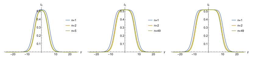
Figure 9: Plot of $I_{0}(\gamma)$ for two-particle states, at $L=10$ (left), $L=100$ (middle) and $L=1000$ (right). If $I_{0}(\gamma)\approx 0$ for all $\gamma\in\mathbb{R}$, the function $Y_{0}^{\blacktriangle}(\gamma)$ is a good approximation of the genuine solution of TBA equations. The height of the plateau is close to $-\frac{1}{2}\,\log(1+y_{0})$ in the left figure.

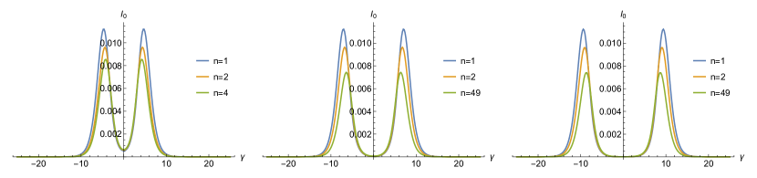
Figure 10: Plot of $I_{0}(\gamma)$ for four-particle states, at $L=10$ (left), $L=100$ (middle) and $L=1000$ (right).

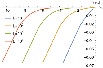
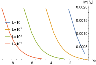
Figure 11: Plot of $I_{0*}(\gamma)$ for two-particle states (left) and four-particle states (right). If $I_{0*}(\gamma)\approx 0$ at $\gamma=\gamma_{s}$  then $\gamma_{s}$ is a good approximation of the genuine Bethe root that solves the exact Bethe equations. We use the same setup as in Figure 9 and 10, respectively.

Corrections to the exact energy.

The exact energy (92) is approximated by

$$\mathcal{E}(L)\simeq\mathcal{E}^{\blacktriangle}(L)=2h\Bigg{(}\sum_{j=1}^{2M}\frac{1}{\cosh(\gamma_{j})}-\int\limits_{-\infty}^{+\infty}\frac{\text{d}\gamma}{\pi}\,\frac{\cosh\gamma}{\sinh^{2}\gamma}\log\left(1+Y^{\blacktriangle}_{0}(\gamma)\right)\Bigg{)}.$$ (363)

It is straightforward to check that the approximate energy becomes close to the energy of free particles when $L\gg 1$ and $n\gg 1$.

Appendix F Numerical results

Here we collect some numerical results for the readers’ convenience.

F.1 $M=1$ energies and Bethe roots

$\nu_{1}$	$\gamma_{1}$	$H_{(1)}^{\nu,L}$
1	1.3698653240	2.0371546985
2	0.3412311709	3.9521799805

Table 2: $M=1$, $L=4$, $N_{0}=2$

$\nu_{1}$	$\gamma_{1}$	$H_{(1)}^{\nu,L}$
1	2.1248622820	1.0028559276
2	1.1089105186	2.4707908032
3	0.5792737159	3.5117487126
4	0.1817026465	4.0386428712

Table 3: $M=1$, $L=8$, $N_{0}=2$

$\nu_{1}$	$\gamma_{1}$	$H_{(1)}^{\nu,L}$
1	2.8618207790	0.4849717915
2	1.8438211035	1.2794684349
3	1.3390651829	2.0126766051
4	0.9929598227	2.6600005573
5	0.7219619376	3.2000441129
6	0.4924934000	3.6163564964
7	0.2870226887	3.8981848212
8	0.0943269199	4.0400428155

Table 4: $M=1$, $L=16$, $N_{0}=2$

$\nu_{1}$	$\gamma_{1}$	$H_{(1)}^{\nu,L}$
1	3.5807368927	0.2368807583
2	2.5603603627	0.6365227133
3	2.0603600910	1.0281132980
4	1.7251311148	1.4082316357
5	1.4710119498	1.7734401398
6	1.2648112263	2.1204079213
7	1.0899414525	2.4459763296
8	0.9368974686	2.7472074554
9	0.7997021734	3.0214244963
10	0.6743276527	3.2662459101
11	0.5579036274	3.4796125862
12	0.4482825396	3.6598056719
13	0.3437821208	3.8054518369
14	0.2430230319	3.9155132154
15	0.1448207412	3.9892619250
16	0.0481100780	4.0262441073

Table 5: $M=1$, $L=32$, $N_{0}=2$

$\nu_{1}$	$\gamma_{1}$	$H_{(1)}^{\nu,L}$	$\nu_{1}$	$\gamma_{1}$	$H_{(1)}^{\nu,L}$
1	4.2879096161	0.1168564842	17	0.8401019031	2.9267028133
2	3.2664446921	0.3155568408	18	0.7742505012	3.0576318067
3	2.7671383824	0.5132072504	19	0.7111470670	3.1811630271
4	2.4341433236	0.7093766819	20	0.6504336814	3.2970173851
5	2.1837123783	0.9036191403	21	0.5918022443	3.4049356209
6	1.9826258225	1.0954854863	22	0.5349845242	3.5046788549
7	1.8143008697	1.2845282941	23	0.4797444118	3.5960290077
8	1.6692618496	1.4703047162	24	0.4258717961	3.6787890734
9	1.5415834217	1.6523785504	25	0.3731776535	3.7527832329
10	1.4273122065	1.8303219179	26	0.3214900533	3.8178568013
11	1.3236779082	2.0037167259	27	0.2706508662	3.8738760127
12	1.2286629854	2.1721559956	28	0.2205130145	3.9207276592
13	1.1407515544	2.3352450966	29	0.1709381451	3.9583186158
14	1.0587748047	2.4926029101	30	0.1217946312	3.9865753002
15	0.9818115704	2.6438629291	31	0.0729558279	4.0054431247
16	0.9091219985	2.7886743016	32	0.0242985168	4.0148860079

Table 6: $M=1$, $L=64$, $N_{0}=2$

F.2 $M=2$ energies and Bethe roots

$\nu_{1}$	$\nu_{3}$	$\gamma_{1}$	$\gamma_{3}$	$H_{(1)}^{\nu,L}$
1	1	2.9376378954	1.8375583252	1.6623510390
1	2	2.6967090197	1.0391156116	3.0495341815
1	3	2.6170173068	0.5539483099	4.0342421895
1	4	2.5887794648	0.1749771889	4.5341663005
2	1	1.0391156116	2.6967090197	3.0495341815
2	2	0.9518480877	1.4877186973	4.4041253580
2	3	1.4462042179	0.5189041649	5.2978941757
2	4	1.4299341712	0.1653301442	5.7541077048
3	1	0.5539483099	2.6170173068	4.0342421895
3	2	0.5189041649	1.4462042179	5.2978941757
3	3	0.4980953042	0.8831783606	6.3729119753
3	4	0.8730916450	0.1592766021	6.7925692823
4	1	0.1749771889	2.5887794648	4.5341663005
4	2	0.1653301442	1.4299341712	5.7541077048
4	3	0.1592766021	0.8730916450	6.7925692823
4	4	0.1555881589	0.4805085942	7.5289149203

Table 7: $M=2$, $L=8$, $N_{0}=2$

$\nu_{1}$	$\nu_{3}$	$\gamma_{1}$	$\gamma_{3}$	$H_{(1)}^{\nu,L}$
1	1	3.6537610671	2.5602970649	0.8203534117
1	2	3.3876886449	1.7628137640	1.6018607650
1	3	3.2857192526	1.3024011789	2.3227799421
1	4	3.2336036393	0.9729210873	2.9591944500
1	5	3.2035863552	0.7101339967	3.4901834518
1	6	3.1856343126	0.4854953019	3.8996058876
1	7	3.1753421098	0.2832967956	4.1768538170
1	8	3.1706273572	0.0931556025	4.3164455616
4	1	0.9729210873	3.2336036393	2.9591944500
4	2	0.9423478941	2.0822853425	3.6872964642
4	3	0.9212795353	1.5406661679	4.3864271809
4	4	0.9059731295	1.1760363379	5.0319943849
4	5	1.1652460981	0.6682476284	5.5204633427
4	6	1.1581088866	0.4598471864	5.8977454073
4	7	1.1537644634	0.2693710960	6.1536717395
4	8	1.1517095215	0.0887380979	6.2827075858
8	1	0.0931556025	3.1706273572	4.3164455616
8	2	0.0912746810	2.0401356906	5.0050489064
8	3	0.0898643130	1.5089325981	5.6697697168
8	4	0.0887380979	1.1517095215	6.2827075858
8	5	0.0878354445	0.8764190409	6.8223972096
8	6	0.0871308216	0.6471361855	7.2716629274
8	7	0.0866115471	0.4457230371	7.6176657203
8	8	0.0862699163	0.2612714949	7.8519608180

Table 8: $M=2$, $L=16$, $N_{0}=2$

$\nu_{1}$	$\nu_{3}$	$\gamma_{1}$	$\gamma_{3}$	$H_{(1)}^{\nu,L}$
1	1	4.3667760502	3.2749047890	0.4030448796
1	2	4.0925190899	2.4758876263	0.8008463492
1	3	3.9835601638	2.0205102633	1.1905732274
1	4	3.9248851827	1.7019564268	1.5688541068
1	5	3.8883291398	1.4559402105	1.9322832043
1	6	3.8635441692	1.2543177294	2.2775537076
1	7	3.8458143772	1.0823054700	2.6015269927
1	8	3.8326777910	0.9311781182	2.9012824112
1	9	3.8227233795	0.7953422171	3.1741580831
1	10	3.8150863070	0.6709773571	3.4177851279
1	11	3.8092099606	0.5553341129	3.6301147693
1	12	3.8047236021	0.4463397930	3.8094360711
1	13	3.8013752502	0.3423611847	3.9543811970
1	14	3.7989931291	0.2420529768	4.0639155381
1	15	3.7974629520	0.1442557986	4.1373126777
1	16	3.7967145735	0.0479245310	4.1741191045
8	1	0.9311781182	3.8326777910	2.9012824112
8	2	0.9216319023	2.7088951040	3.2779452910
8	3	0.9141849574	2.1842219252	3.6517239986
8	4	0.9079885188	1.8364873234	4.0183658379
8	5	0.9027267397	1.5744210131	4.3743620916
8	6	0.8982298328	1.3626539505	4.7164383992
8	7	0.8943850814	1.1837177617	5.0414825239
8	8	0.8911070856	1.0276784945	5.3465517214
8	9	1.0249251329	0.7638168954	5.6053929680
8	10	1.0226557697	0.6461621688	5.8365914251
8	11	1.0208101070	0.5359482231	6.0381767125
8	12	1.0193396941	0.4314761487	6.2084956100
8	13	1.0182063344	0.3313762548	6.3462183473
8	14	1.0173808114	0.2344982199	6.4503309849
8	15	1.0168419384	0.1398351973	6.5201144774
8	16	1.0165759091	0.0464692922	6.5551150808

Table 9: $M=2$, $L=32$, $N_{0}=2$

F.3 $N_{0}\neq 2$ energies and Bethe roots

$N_{0}$	$\nu_{1}$	$\gamma_{1}$	$H_{(1)}^{\nu,L}$	$N_{0}$	$\nu_{1}$	$\gamma_{1}$	$H_{(1)}^{\nu,L}$
1	1	2.1478952374	0.9635873862	4	1	2.0953342432	1.0566264100
1	2	1.1133031093	2.4362266137	4	2	1.1031296462	2.5183340592
1	3	0.5807795815	3.4803921364	4	3	0.5772837367	3.5550539708
1	4	0.1820951353	4.0088079500	4	4	0.1811833307	4.0799379863

Table 10: $M=1$, $L=8$, $N_{0}=1$ or $N_{0}=4$

$N_{0}$	$\nu_{1}$	$\gamma_{1}$	$H_{(1)}^{\nu,L}$	$N_{0}$	$\nu_{1}$	$\gamma_{1}$	$H_{(1)}^{\nu,L}$
1	1	2.8857343672	0.4654209354	4	1	2.8311082468	0.5117915477
1	2	1.8488625594	1.2606517243	4	2	1.8371707568	1.3053067737
1	3	1.3412153995	1.9945438917	4	3	1.3362158215	2.0376028122
1	4	0.9941067817	2.6424719775	4	4	0.9914373805	2.6841218621
1	5	0.7226306849	3.1830157305	4	5	0.7210735368	3.2234992687
1	6	0.4928863986	3.5997081486	4	6	0.4919710848	3.6393056282
1	7	0.2872311467	3.8817888137	4	7	0.2867455680	3.9207979770
1	8	0.0943923424	4.0237715433	4	8	0.0942399382	4.0624898925

Table 11: $M=1$, $L=16$, $N_{0}=1$ or $N_{0}=4$

References

- (1) J.M. Maldacena, The Large N limit of superconformal field theories and supergravity, Adv. Theor. Math. Phys. 2 (1998) 231 [hep-th/9711200].
- (2) A.S. Haupt, S. Lautz and G. Papadopoulos, A non-existence theorem for supersymmetric AdS3 backgrounds, JHEP 07 (2018) 178 [1803.08428].
- (3) F. Larsen and E.J. Martinec, U(1) charges and moduli in the D1 - D5 system, JHEP 06 (1999) 019 [hep-th/9905064].
- (4) O. Ohlsson Sax and B. Stefański, Closed strings and moduli in AdS3/CFT2, JHEP 05 (2018) 101 [1804.02023].
- (5) A. Giveon, D. Kutasov and N. Seiberg, Comments on string theory on AdS(3), Adv. Theor. Math. Phys. 2 (1998) 733 [hep-th/9806194].
- (6) J.M. Maldacena and H. Ooguri, Strings in AdS(3) and SL(2,R) WZW model 1.: The Spectrum, J. Math. Phys. 42 (2001) 2929 [hep-th/0001053].
- (7) N. Berkovits, C. Vafa and E. Witten, Conformal field theory of AdS background with Ramond-Ramond flux, JHEP 03 (1999) 018 [hep-th/9902098].
- (8) L. Eberhardt, M.R. Gaberdiel and R. Gopakumar, The Worldsheet Dual of the Symmetric Product CFT, JHEP 04 (2019) 103 [1812.01007].
- (9) G. Giribet, C. Hull, M. Kleban, M. Porrati and E. Rabinovici, Superstrings on AdS3 at 1, JHEP 08 (2018) 204 [1803.04420].
- (10) L. Eberhardt, A perturbative CFT dual for pure NS–NS AdS3 strings, J. Phys. A 55 (2022) 064001 [2110.07535].
- (11) D. Berenstein and R.G. Leigh, Superstring perturbation theory and Ramond-Ramond backgrounds, Phys. Rev. D 60 (1999) 106002 [hep-th/9904104].
- (12) M. Cho, S. Collier and X. Yin, Strings in Ramond-Ramond Backgrounds from the Neveu-Schwarz-Ramond Formalism, JHEP 12 (2020) 123 [1811.00032].
- (13) L. Eberhardt and K. Ferreira, The plane-wave spectrum from the worldsheet, JHEP 10 (2018) 109 [1805.12155].
- (14) G. Arutyunov and S. Frolov, Foundations of the AdS Superstring. Part I, J. Phys. A 42 (2009) 254003 [0901.4937].
- (15) N. Beisert et al., Review of AdS/CFT Integrability: An Overview, Lett. Math. Phys. 99 (2012) 3 [1012.3982].
- (16) A. Sfondrini, Towards integrability for , J. Phys. A 48 (2015) 023001 [1406.2971].
- (17) A. Cagnazzo and K. Zarembo, B-field in AdS(3)/CFT(2) Correspondence and Integrability, JHEP 11 (2012) 133 [1209.4049].
- (18) S. Frolov, D. Polvara and A. Sfondrini, On mixed-flux worldsheet scattering in AdS3/CFT2, 2306.17553.
- (19) S. Frolov and A. Sfondrini, New dressing factors for AdS3/CFT2, JHEP 04 (2022) 162 [2112.08896].
- (20) S. Frolov and A. Sfondrini, Mirror thermodynamic Bethe ansatz for AdS3/CFT2, JHEP 03 (2022) 138 [2112.08898].
- (21) A. Cavaglià, N. Gromov, B. Stefański, Jr., Jr. and A. Torrielli, Quantum Spectral Curve for AdS3/CFT2: a proposal, JHEP 12 (2021) 048 [2109.05500].
- (22) J.A. Minahan and K. Zarembo, The Bethe ansatz for N=4 superYang-Mills, JHEP 03 (2003) 013 [hep-th/0212208].
- (23) A. Brollo, D. le Plat, A. Sfondrini and R. Suzuki, Tensionless Limit of Pure–Ramond-Ramond Strings and AdS3/CFT2, Phys. Rev. Lett. 131 (2023) 161604 [2303.02120].
- (24) T. Lloyd, O. Ohlsson Sax, A. Sfondrini and B. Stefański, Jr., The complete worldsheet S matrix of superstrings on AdS S T4 with mixed three-form flux, Nucl. Phys. B 891 (2015) 570 [1410.0866].
- (25) F.K. Seibold and A. Sfondrini, Transfer matrices for AdS3/CFT2, JHEP 05 (2022) 089 [2202.11058].
- (26) S. Frolov, A. Pribytok and A. Sfondrini, Ground state energy of twisted superstring and the TBA, 2305.17128.
- (27) G. Arutyunov and S. Frolov, String hypothesis for the AdS(5) x S**5 mirror, JHEP 03 (2009) 152 [0901.1417].
- (28) S. Frolov and A. Sfondrini, to appear, xxxx.xxxxx.
- (29) A. Fontanella and A. Torrielli, Geometry of Massless Scattering in Integrable Superstring, JHEP 06 (2019) 116 [1903.10759].
- (30) G. Arutyunov and S. Frolov, On String S-matrix, Bound States and TBA, JHEP 12 (2007) 024 [0710.1568].
- (31) S. Frolov and A. Sfondrini, Massless S matrices for AdS3/CFT2, JHEP 04 (2022) 067 [2112.08895].
- (32) P. Dorey and R. Tateo, Excited States by Analytic Continuation of TBA Equations, Nucl. Phys. B 482 (1996) 639 [hep-th/9607167].
- (33) M. Baggio, O. Ohlsson Sax, A. Sfondrini, B. Stefański and A. Torrielli, Protected string spectrum in AdS3/CFT2 from worldsheet integrability, JHEP 04 (2017) 091 [1701.03501].
- (34) S.J. van Tongeren, Introduction to the thermodynamic Bethe ansatz, J. Phys. A 49 (2016) 323005 [1606.02951].
- (35) A.B. Zamolodchikov, On the thermodynamic Bethe ansatz equations for reflectionless ADE scattering theories, Phys. Lett. B 253 (1991) 391.
- (36) L. Frappat, A. Sciarrino and P. Sorba, Structure of Basic Lie Superalgebras and of Their Affine Extensions, Commun. Math. Phys. 121 (1989) 457.
- (37) D. Chapovalov, M. Chapovalov, A. Lebedev and D. Leites, The Classification of almost affine (hyperbolic) Lie superalgebras, J. Nonlin. Math. Phys. 17 (2010) 103 [0906.1860].
- (38) A. Zamolodchikov, Thermodynamic bethe ansatz in relativistic models: Scaling 3-state potts and lee-yang models, Nuclear Physics B 342 (1990) 695.
- (39) S.J. van Tongeren, Introduction to the thermodynamic bethe ansatz, Journal of Physics A: Mathematical and Theoretical 49 (2016) 323005.
- (40) S. Frolov and R. Suzuki, Temperature quantization from the TBA equations, Phys. Lett. B 679 (2009) 60 [0906.0499].
- (41) D. Tong, The holographic dual of , JHEP 04 (2014) 193 [1402.5135].
- (42) R. Borsato, O. Ohlsson Sax, A. Sfondrini and B. Stefański, The worldsheet S matrix, J. Phys. A 48 (2015) 415401 [1506.00218].
- (43) S. Ekhammar and D. Volin, Monodromy bootstrap for SU(2|2) quantum spectral curves: from Hubbard model to AdS3/CFT2, JHEP 03 (2022) 192 [2109.06164].
- (44) A. Cavaglià, S. Ekhammar, N. Gromov and P. Ryan, Exploring the Quantum Spectral Curve for AdS3/CFT2, 2211.07810.
- (45) G. Arutyunov, S. Frolov and R. Suzuki, Exploring the mirror TBA, JHEP 05 (2010) 031 [0911.2224].
- (46) G. Arutyunov and S. Frolov, The Dressing Factor and Crossing Equations, J. Phys. A 42 (2009) 425401 [0904.4575].
- (47) N. Beisert, R. Hernandez and E. Lopez, A Crossing-Symmetric Phase for Strings, JHEP 11 (2006) 070 [hep-th/0609044].
- (48) S. Frolov, Konishi operator at intermediate coupling, J. Phys. A 44 (2011) 065401 [1006.5032].