Looking into the faintEst WIth MUSE (LEWIS): on the nature of ultra-diffuse galaxies in the Hydra-I cluster

Looking into the faintEst WIth MUSE (LEWIS) is an ESO large observing programme aimed at obtaining the first homogeneous integral-field spectroscopic survey of 30 extremely low-surface brightness (LSB) galaxies in the Hydra I cluster of galaxies, with MUSE at ESO-VLT. The majority of LSB galaxies in the sample (22 in total) are ultra-diffuse galaxies (UDGs). Data acquisition started in December 2021 and is expected to be concluded by March 2024. Until June 2023, 29 targets were observed and the redshift derived for 20 of them. The distribution of systemic velocities $V_{\rm sys}$ ranges between 2317 km/s and 5198 km/s and is centred on the mean velocity of Hydra I ($V_{\rm sys}=3683\pm 46$ km/s). Considering the mean velocity and the velocity dispersion of the cluster ($\sigma_{\rm cluster}\sim 700$ km/s), 17 out of 20 targets are confirmed cluster members. The three objects with velocities more than $2\sigma_{\rm cluster}$ distant from the cluster mean velocity could be two background and one foreground galaxies. To assess the quality of the data and demonstrate the feasibility of the science goals, we report the preliminary results obtained for one of the sample galaxies, UDG11. For this target, we i) derived the stellar kinematics, including the 2-dimensional maps of line-of-sight velocity and velocity dispersion, ii) constrained age and metallicity, and iii) studied the globular cluster (GC) population hosted by the UDG. Results are compared with the available measurements for UDGs and dwarf galaxies in literature. By fitting the stacked spectrum inside one effective radius, we find that UDG11 has a velocity dispersion $\sigma=20\pm 8$ km/s, it is old ($10\pm 1$ Gyr), metal-poor ([$M$/H]$=-1.17\pm 0.11$ dex) and has a total dynamical mass-to-light ratio M$/L_{V}\sim 14$, comparable to those observed for classical dwarf galaxies. The spatially resolved stellar kinematics maps suggest that UDG11 does not show a significant velocity gradient along either major or minor photometric axes, and the average value of the velocity dispersion is $\langle\sigma\rangle_{\rm e}=27\pm 8$ km/s. We find two GCs kinematically associated with UDG11. The estimated total number of GCs in UDG11, corrected for the spectroscopic completeness limit, is $N_{\rm GC}=5.9^{+2.2}_{-1.8}$, which corresponds to a GC specific frequency of $S_{N}=8.4^{+3.2}_{-2.7}$.

1 Introduction

Ultra-diffuse galaxies (UDGs) are among the faintest and lowest surface brightness ($\mu_{0,g}\geq 24$ mag arcsec^-2, $R_{\rm e}\geq 1.5$ kpc) galaxies known in the universe. Very low surface brightness (LSB) galaxies are known since the 80s, they were discovered in the Virgo and Fornax clusters decades ago (Sandage & Binggeli, 1984; Impey et al., 1988; Ferguson & Sandage, 1988; Bothun et al., 1991). The term UDG was introduced by van Dokkum et al. (2015), who detected several galaxies, including an extremely faint and diffuse galaxy, named DF44, in the Coma cluster, having an effective radius $R_{\rm e}\sim 4.3$ kpc, similar to that of the Milky-Way ($R_{\rm e}\sim 4.5$ kpc), but with a stellar mass 100 times smaller.

To survive cluster tides, being so diffuse and faint, UDGs should host a large amount of dark matter (van Dokkum et al., 2015). This idea triggered an ever-increasing attention to the detection and study of UDGs and gave to these galaxies a special role in the realm of the LSB universe. Given the extremely low baryonic mass density, UDGs are indeed considered particularly suitable laboratories to test the formation of galaxies in the $\Lambda$-Cold Dark Matter ($\Lambda$CDM) framework.

Since 2015, several observational campaigns have been carried out to get deep images, mapping different environments from groups to clusters of galaxies, which provided large samples of LSB galaxies, including UDGs (Yagi et al., 2016; van der Burg et al., 2017; Trujillo et al., 2017; Venhola et al., 2017; Janssens et al., 2019; Mancera Piña et al., 2019a; Prole et al., 2019a; Román et al., 2019; Lim et al., 2020; Marleau et al., 2021; La Marca et al., 2022a; Zaritsky et al., 2022).

To classify an LSB galaxy as UDG, the most conservative approach is based on the empirical definition proposed by van Dokkum et al. (2015). This requires UDGs to have a central surface brightness fainter than 24 mag arcsec^-2 (in the $g$ band) and an effective radius larger than 1.5 kpc. However, other criteria have also been proposed which used different cuts in size and/or surface brightness limits (Koda et al., 2015; Yagi et al., 2016; van der Burg et al., 2017; Mancera Piña et al., 2019b). In particular, taking advantage of a large and statistically significant sample of dwarf and LSB galaxies in the Virgo cluster, Lim et al. (2020) found that UDGs can be classified as the extremes in the broad scaling relationships between photometric and structural properties of LSB galaxies (e.g., total luminosity vs. $R_{\rm e}$ and $\mu_{\rm e}$). UDGs turn out to be $\sim 2.5\sigma$ fainter and larger than the average distribution of the parent dwarf galaxy sample. These results support the idea that UDGs can be considered as extreme LSB tail of the size-luminosity distribution of dwarf galaxies.

The considerable amount of imaging data collected to date for UDGs has shown that these galaxies span a wide range of structural and photometric properties. Based on their integrated colours, it seems that two populations of UDGs exist. Red UDGs are mainly found in clusters of galaxies, while bluer objects are discovered in the low-density regions, i.e. the outskirts of clusters and in the field (see e.g. Román & Trujillo, 2017; Leisman et al., 2017; Prole et al., 2019b; Marleau et al., 2021). Red UDGs are also found in groups of galaxies (Marleau et al., 2021).

Deep images have also allowed the detection and study of globular cluster (GC) populations in UDGs. By deriving the GC specific frequency ($S_{N}=N_{\rm GC}\times 10^{0.4(M_{V}+15)}$, Harris & van den Bergh, 1981), observations from space and ground-based telescopes have revealed an extreme degree of variability of $S_{N}$ values. Some UDGs are consistent with having no GCs population, while others present $S_{N}$ as high as $\sim$150 (Prole et al., 2019a; Saifollahi et al., 2021, 2022; Marleau et al., 2021; La Marca et al., 2022a). The unusually high $S_{N}$ in some UDGs triggered a debate about the fraction of DM in UDGs. Assuming that the relation between the total number of GCs, $N_{\rm GC}$, and the host galaxy’s halo virial mass, valid from giant to dwarf galaxies (see Burkert & Forbes, 2020, and references therein), also holds in the LSB regime, UDGs with large $N_{\rm GC}$ values might be DM-dominated systems, with halo masses 100 times more massive ($M_{\rm h}\geq 10^{11}$  M_⊙) than higher surface brightness dwarf galaxies of similar luminosity.

To date, the DM content of the UDGs is a highly debated topic. The few spectroscopic studies, focusing on special cases, point to a rather diverse population. Some UDGs were found to host a very massive DM halo (Toloba et al., 2018; van Dokkum et al., 2019; Forbes et al., 2021; Gannon et al., 2021), while at the same time, there are some UDGs with a “normal” DM halo, i.e. having the DM content consistent with that of other dwarf galaxies of similar luminosity. Finally, a few UDGs have also been discussed to populate the opposite extreme, being basically DM-free (van Dokkum et al., 2018; Collins et al., 2021).

Because of their LSB nature, getting spectroscopic data for UDGs is a challenging task. To date, as opposed to the deep images available, we still lack a statistically significant sample of UDGs with spectroscopy, which strongly limits our constraints and conclusions on their stellar populations and DM content. For only two to three dozen of UDGs, the available spectroscopic studies reveal the existence of both, metal-poor ($-0.5\leq[M$/H$]\leq-1.5$ dex) and old systems ($\sim$9 Gyr; e.g., Ferré-Mateu et al., 2018; Pandya et al., 2018; Fensch et al., 2019), as well as younger star-forming UDGs (Martín-Navarro et al., 2019). The kinematic measurements of UDGs available in groups and clusters suggest that the rotation velocity of stars is very low (see Gannon et al., 2023, and references therein).

The wide range of photometric and spectroscopic properties, including the GCs content, do not fit into a single formation scenario, and there is a general consensus that different formation channels can be invoked to form galaxies with UDG-like properties. van Dokkum et al. (2015) coined the term “failed” galaxies, suggesting that these objects with high DM content and large effective radii might have lost gas supply at an early epoch, evolving to become quenched and diffuse galaxies. Nowadays, a plethora of UDG formation mechanisms have been proposed, which are nicely able to form a galaxy with the typical morphology of UDGs, but they predict different DM amounts, age and metallicity, and gas content. It has to be shown which formation scenarios are most consistent with the observational properties of UDGs.

For simplicity, formation scenarios for UDGs can be divided into two groups, based on the physical processes at work: internal and external mechanisms.

Star-formation feedback and highly rotating DM halos are both possible internal mechanisms that can form large and diffuse galaxies. In the former case, repeated star formation episodes during early galaxy evolution can drive the gas out to large radii and prevent the subsequent star formation (Di Cintio et al., 2017). In the latter case, the high specific angular momentum of a DM halo prevents gas from effectively collapsing into a dense structure (Amorisco & Loeb, 2016; Rong et al., 2017; Tremmel et al., 2019). In both scenarios, the resulting UDGs are gas-rich and have a “normal”, dwarf-like DM halo.

Gravitational interactions and merging between galaxies, as well as interactions with the environment, are external processes that might shape galaxies to become UDG-like. Similar to the tidal dwarf galaxies (TDGs), UDGs might originate from the collisional debris of a merger (Lelli et al., 2015; Duc et al., 2014; Ploeckinger et al., 2018). Poggianti et al. (2019) suggested that UDGs might form from ram pressure-stripped gas clumps in the extended tails of infalling cluster galaxies. Both scenarios predict blue, dusty, star-forming, and DM-free UDGs, with moderate to low metallicity and UV emission. Weak tidal interaction of a dwarf galaxy with a massive nearby giant galaxy has also been addressed as a possible mechanism to form a UDG (Conselice, 2018; Carleton et al., 2021; Bennet et al., 2018; Müller et al., 2019; Gannon et al., 2021). High-velocity galaxy collisions might generate several debris, where some of them could remain gravitationally-bound systems with a UDG-like structure (Silk, 2019; Shin et al., 2020; van Dokkum et al., 2022). Also in these latter cases, the formed UDGs are expected to be DM-free galaxies, but red and gas-poor systems. UDGs could also form from large dwarf galaxies, which, during their interaction with the cluster environment, got their gas removed by ram pressure stripping, and thus halting subsequent star formation (Yozin & Bekki, 2015; Tremmel et al., 2020). The resulting UDG is gas-poor and has a dwarf-like DM content. Finally, in the framework of external processes, a quenched, isolated, gas-poor UDG, with a dwarf-like DM halo, might result as a backsplash galaxy. In this case, former satellites of a group or cluster halo in an early epoch, are now found a few megaparsecs away from them (Benavides et al., 2021). All the above scenarios and related predicted properties for UDGs are summarised in Fig. 1.

Based on the IllustrisTNG simulations, Sales et al. (2020) proposed two different formation channels for cluster UDGs. A population of “Born-UDGs” (B-UDGs) could form in the field and later enter the cluster environment. The B-UDGs originate from LSB galaxies that, once having joined the cluster potential, lost their gas supply and quench. Differently, tidal forces could act on luminous galaxies in the cluster, removing their DM and puffing up their stellar component. As a consequence, these galaxies evolve into UDGs, and they are named “Tidal-UDGs” (T-UDGs). T-UDGs populate the centre of the clusters and, at a given stellar mass, have lower velocity dispersion, higher metallicity and lower DM fraction with respect to the B-UDGs.

In summary, observations strongly suggest that the class of UDGs might comprise different types of galaxies, with different intrinsic properties (e.g., colours, stellar populations, and DM fractions). Theoretical works on UDGs, also reviewed above, show that more than one formation channel might exist to account for the different types of UDGs, or, reasonably, a combination of physical processes to account also for environmental effects. The lack of stellar kinematics and stellar population properties is the main limitation to provide stringent conclusions on the nature of UDGs and to discriminate between the formation channels.

In this paper, we present the “Looking into the faintEst WIth MUSE” (LEWIS) project, which aims at obtaining the first homogeneous integral-field spectroscopic survey of 30 extreme LSB galaxies, including UDGs, in the Hydra I cluster of galaxies, with MUSE at ESO-VLT. Doubling the number of spectroscopically studied UDGs, with this project we will make a decisive impact in this field. With LEWIS we will map, for the first time, the stellar population and DM content of a complete sample of UDGs in a galaxy cluster, based on spectroscopic data.

The paper is organised as follows. The galaxy sample and science goals of the LEWIS project are presented in Sec. 2. Observations and data reduction are described in Sec. 3. The redshift estimates for all the so far observed sample UDGs are provided in Sec. 4. In Sec. 5 we show the analysis of the MUSE data, with a detailed description for one of the galaxies in the sample, UDG11, chosen as test case. The preliminary results are discussed in Sec. 6, and conclusions are provided in Sec. 7.

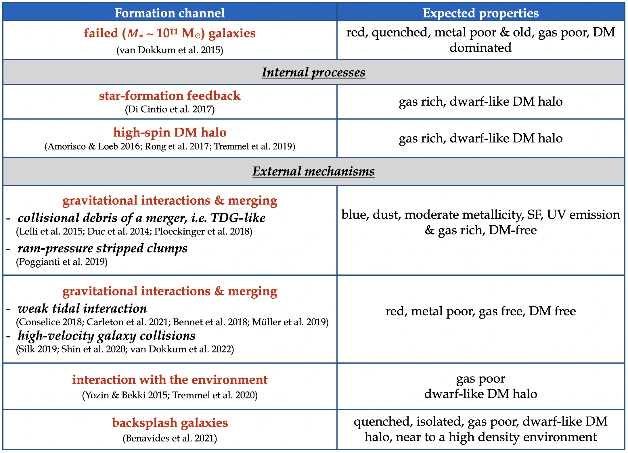
Figure 1: Schematic view of the main formation channels proposed for UDGs. In the left boxes are listed the relevant physical processes. The predicted properties for UDGs, from each formation channel, are reported in the boxes on the right.

2 Galaxy sample and science goals of the LEWIS project

LEWIS is an ESO Large Programme, started in 2021, approved during the ESO period 108 (P.I. E. Iodice, ESO programme ID 108.222P), to obtain the first homogeneous integral-field spectroscopic survey of UDGs in the Hydra I cluster of galaxies (see Fig. 2). This is a rich environment of galaxies, located in the southern hemisphere at a distance of $51\pm 6$ Mpc (Christlein & Zabludoff, 2003), with a virial mass of $2\times 10^{14}$ M_⊙ (Girardi et al., 1998), a virial radius $R_{\rm vir}\sim 1.6$ Mpc, and a velocity dispersion of $\sigma_{\rm cluster}\simeq 700$ km/s (Lima-Dias et al., 2021). Hydra I has been extensively studied using deep images and multi-object spectroscopy (e.g., Misgeld et al., 2008, 2011; Richtler et al., 2011; Arnaboldi et al., 2012; Hilker et al., 2018; Barbosa et al., 2018, 2021). Main results show that this cluster is still in an active phase of mass assembly, since ongoing interactions are detected around the brightest cluster member NGC 3311 (see Barbosa et al., 2018; Iodice et al., 2021, and references therein). The projected distribution of all cluster members, bright galaxies and dwarfs, shows three main over-densities: the core of the cluster, around NGC 3311 and NGC 3309, a sub-group of galaxies elongated North-South and a sub-group of galaxies in the South-East (La Marca et al., 2022a).

The latest Hydra I catalogue presented 317 galaxies fainter than $M_{r}>-18.5$ mag and semi-major axis larger than  200 pc, of which about 230 new candidates have been recently discovered by Iodice et al. (2020, 2021) and La Marca et al. (2022b, a). The authors studied the photometric properties of this class of objects, which are briefly summarised below. According to the colour-magnitude relation for early-type giant and dwarf galaxies in Hydra I (Misgeld et al., 2008), all of the new candidates are consistent with being cluster members. In this sample, according to the definition proposed by van Dokkum et al. (2015), i.e. $R_{\rm e}\geq 1.5$ kpc and $\mu_{0,g}\geq 24$ mag/arcsec², 22 objects are classified as UDGs (Iodice et al., 2020, 2021; La Marca et al., 2022a). Additional 10 galaxies are very extended ($R_{\rm e}\geq 1.5$ kpc), but with $\mu_{0,g}\geq 23$ mag/arcsec², were classified as LSB dwarfs. Taking into account the virial mass of $\sim 10^{14}$ M_⊙ for the Hydra I cluster (see Fig. 6 in La Marca et al., 2022a), and the UDG abundance-halo mass relation ($N_{\rm UDG}\propto M_{200}^{1.11}$, van der Burg et al., 2017), the expected number of UDGs in Hydra I within $1R_{\rm vir}$ is $48\pm 10$ UDGs. Therefore, the detection of 22 UDGs inside $\simeq 0.4R_{\rm vir}$ of the Hydra I cluster can be considered a complete sample for this class of objects. Based on photometric and size selection, GC candidates are identified around a few of those LSB galaxies, with a total number of GCs per galaxy $N_{\rm GC}\geq 2$.

The newly discovered LSB dwarfs and UDGs span a wide range of central surface brightness ($23\leq\mu_{0,g}\leq 27$ mag/arcsec²) and effective radius ($1\leq R_{\rm e}\leq 4$ kpc). Compared to the population of early-type dwarf galaxies in the cluster, they have similar integrated $g-r$ colours, $0.4\leq g-r\leq 0.9$ mag, and stellar masses $M_{\star}=5\times 10^{6}-2\times 10^{8}$ M_⊙. Inside $\simeq 0.4R_{\rm vir}$ of the Hydra I cluster, the structural and photometric parameters (i.e., surface brightness, size, color, and Sersic n-index) and GC content of all LSB galaxies have similar properties and trends to those observed for dwarf galaxies. Therefore, as addressed by La Marca et al. (2022a), these findings suggest that a single population of LSB galaxies is present in this region of the cluster, and UDGs can be reasonably considered as the extreme LSB tail of the size–luminosity distribution of all dwarfs in this environment. Finally, the LSB galaxies share a similar 2D projected distribution as observed for the dwarf and giant galaxies in the cluster: over-densities are found in the cluster core and north of the cluster centre. Similar results are found for other galaxy clusters, where over-densities of UDGs are observed close to subgroups of other cluster members (see e.g. Janssens et al., 2019). Observing UDGs spatially associated with groups infalling onto the cluster, would further support the idea that they might follow two formation paths, as proposed by Sales et al. (2020). As a conclusive remark, the previous results and ongoing studies on UDGs in Hydra I suggest that this environment offers a unique opportunity to analyse this class of LSB galaxies in great detail.

The UDGs’ nature and formation can be addressed by measuring their kinematics, stellar population and DM content as a function of their location in the cluster. Compared to the Coma cluster, the so far best-studied environment where UDGs have been investigated, Hydra I is at half of Coma’s distance and it is 10 times less massive. Therefore, Hydra I offers the exquisite opportunity to analyse LSB galaxies, including UDGs, in an environment of different mass scales, and relate their properties to the mass assembly processes. In particular, if the new spectroscopic data from the LEWIS project confirm the asymmetric distribution of UDGs, we can investigate whether the galaxies in the subgroups have different properties from those in the outskirts of the cluster, indicating that the latter systems have formed as genuine UDGs different from those in the denser inner environment.

Given the large variety of observed properties (mainly based on deep images) and theoretical predictions, the LEWIS project will provide a notable boost in our knowledge of UDG structure and formation in a cluster environment (see Forbes et al., 2023). In particular, we expect to address the following science goals, which are the main debated issues on the nature of UDGs:

• DM content in each UDG of the sample through dynamical mass estimates from stellar kinematics. Since the UDGs are not uniformly distributed inside the cluster, we will check if the DM content correlates with the environment in which the UDG resides;

• UDGs’ star formation history from SED fitting of their integrated spectra. This allows to study the evolutionary link between the UDGs and other dwarf galaxies through a comparison of their stellar population and structural properties;

• The spectroscopic confirmation of GC candidates around UDGs will improve their ${S_{N}}$ estimates, which in turn will put on a firmer basis the discussion about possible overdensities of GCs around some UDGs and the relation to the host galaxy DM content.

To these aims, the main objectives of LEWIS are to derive the stellar kinematics, stellar populations and the spectroscopic specific frequency ${S_{N}}$ of the hosted GCs, for all the selected galaxies in our sample. As stated in Sec. 1, similar studies are available only for about 35 UDGs in total, mainly in the Coma cluster (van Dokkum et al., 2017; Ruiz-Lara et al., 2018; Ferré-Mateu et al., 2018; Gu et al., 2018). In particular, integral-field (IF) spectroscopy is available only for about a dozen UDGs (Martín-Navarro et al., 2019; Emsellem et al., 2019; Müller et al., 2020; Gannon et al., 2021; Webb et al., 2022; Gannon et al., 2023).

From the sample of 32 LSB galaxies, photometrically detected in the Hydra I cluster (Iodice et al., 2020; La Marca et al., 2022a), we have selected 30 objects (22 UDGs and 8 LSB galaxies) for the spectroscopic follow-up with MUSE at ESO-VLT within our LEWIS project. They were selected to have an effective surface brightness in the range $25\leq\mu_{\rm e}\leq 27.5$ mag/arcsec² in the $g$ band, which provides the minimum signal-to-noise ratio (SNR$\sim$5-10, depending on the surface brightness) per spaxel in a reasonable integration time ($\sim$2-6 hours), required for the main goals of this project. The two targets excluded from the spectroscopic LEWIS follow-up, UDG14 and UDG19 in La Marca et al. (2022a), are the faintest objects of the photometric sample with $\mu_{\rm e}=28.5$ mag/arcsec² in the $g$ band. According to the color-magnitude relation (see Fig. 3 in La Marca et al., 2022a), both galaxies can be considered as Hydra I cluster members. Galaxies in the LEWIS sample are listed in Table 1 and shown in Fig. 2.

Table 1: LEWIS sample: UDG and LSB galaxies in the Hydra I cluster.

Object	R.A.	DEC	$M_{r}$	$M_{*}$	$\mu_{\rm e}$	$\mu_{0}$	$R_{\rm e}$	$N_{\rm GC}$	Obs. Status	Exp. Time	$V_{\rm sys}$
	[J2000]	[J2000]	[mag]	[$10^{8}$ M${}_{\odot}]$	[mag/arcsec2]	[mag/arcsec2]	[kpc]			[hrs]	[km/s]
(1)	(2)	(3)	(4)	(5)	(6)	(7)	(8)	(9)	(10)	(11)	(12)
UDG 1	10:37:54.12	-27:09:37.50	-15.48	1.12	25.2$\pm$0.1	24.2$\pm$0.1	1.75$\pm$0.12	0$\pm$1	C	2.00	4219$\pm$9
UDG 2	10:37:34.89	-27:10:29.94	-14.27	0.55	26.2$\pm$0.1	25.0$\pm$0.1	1.55$\pm$0.12	7$\pm$3	P	1.33	-
UDG 3	10:36:58.63	-27:08:10.21	-14.70	1.65	26.1$\pm$0.2	25.2$\pm$0.2	1.88$\pm$0.12	15$\pm$6	C	3.00	3550$\pm$26
UDG 4	10:37:02.64	-27:12:15.01	-16.03	10.6	25.8$\pm$0.1	24.9$\pm$0.1	2.64$\pm$0.12	2$\pm$1	C	2.00	2317$\pm$13
UDG 5	10:36:07.68	-27:19:03.26	-14.66	1.16	25.3$\pm$0.3	23.7$\pm$0.3	1.42$\pm$0.12	0$\pm$1	S	-	-
UDG 6	10:36:35.80	-27:19:36.12	-14.38	0.32	25.3$\pm$0.1	24.1$\pm$0.1	1.37$\pm$0.12	0$\pm$1	P	0.75	-
UDG 7	10:36:37.16	-27:22:54.93	-13.72	0.49	26.9$\pm$0.4	24.4$\pm$0.4	1.66$\pm$0.12	3$\pm$1	C	3.80	4134$\pm$28
UDG 8	10:38:14.59	-27:24:27.07	-14.87	0.53	25.0$\pm$0.6	23.2$\pm$0.6	1.40$\pm$0.12	0$\pm$1	P	0.75	4793$\pm$16
UDG 9	10:37:22.85	-27:36:02.80	-15.16	1.78	26.8$\pm$0.2	24.2$\pm$0.2	3.46$\pm$0.12	7$\pm$1	C	3.90	4302$\pm$13
UDG 10	10:35:27.32	-27:33:03.86	-13.89	0.26	27.3$\pm$0.3	24.3$\pm$0.3	2.29$\pm$0.10	0$\pm$1	C	3.85	3577$\pm$139
UDG 11	10:34:59.55	-27:25:37.95	-14.75	0.63	25.7$\pm$0.1	24.4$\pm$0.1	1.66$\pm$0.12	7$\pm$3	C	6.10	3507$\pm$3
UDG 12	10:36:45.55	-27:48:12.73	-14.30	1.19	26.2$\pm$0.2	25.1$\pm$0.2	1.64$\pm$0.12	0$\pm$1	P	1.50	4615$\pm$13
UDG 13	10:36:14.49	-27:30:26.60	-12.73	0.20	27.3$\pm$0.1	24.2$\pm$0.2	1.60$\pm$0.20	-	C	3.93	3438$\pm$52
UDG 15	10:36:02.55	-27:36:19.57	-11.95	0.06	27.7$\pm$0.2	25.0$\pm$0.3	1.51$\pm$0.15	2$\pm$3	C	4.68	3553$\pm$88
UDG 16	10:36:25.30	-27:14:14.74	-12.84	0.11	27.6$\pm$0.1	25.9$\pm$0.2	1.75$\pm$0.12	-	S	-	-
UDG 17	10:36:41.72	-27:16:37.48	-13.99	1.20	26.7$\pm$0.1	24.9$\pm$0.1	1.50$\pm$0.20	3$\pm$3	P	1.50	-
UDG 18	10:36:16.82	-27:20:16.84	-12.28	0.09	27.6$\pm$0.2	25.6$\pm$0.2	1.64$\pm$0.12	11$\pm$7	C	4.70	-
UDG 20	10:38:04.43	-27:29:50.18	-12.95	0.14	27.3$\pm$0.1	26.0$\pm$0.3	1.97$\pm$0.12	-	C	3.88	4693$\pm$12
UDG 21	10:36:54.17	-27:36:55.07	-12.78	0.11	27.3$\pm$0.5	24.0$\pm$0.4	1.50$\pm$0.12	-	C	3.88	3489$\pm$22
UDG 22	10:34:40.97	-27:42:03.27	-13.92	0.36	26.5$\pm$0.1	25.3$\pm$0.2	3.60$\pm$0.12	-	P	1.50	5198$\pm$5
UDG 23	10:35:27.70	-27:46:16.58	-14.11	0.34	27.2$\pm$0.2	24.3$\pm$0.3	2.47$\pm$0.20	-	C	2.10	3496$\pm$33
UDG $32$	10:37:04.20	-27:42:53.92	-14.65	8.00	27.5$\pm$1.0	26.2$\pm$1.0	3.80$\pm$1.00	7$\pm$4	C	5.00	-
LSB 1	10:36:00.03	-27:28:58.17	-12.38	0.06	26.6$\pm$0.1	23.9$\pm$0.2	0.81$\pm$0.90	-	S	-	-
LSB 2	10:36:09.65	-27:30:51.61	-12.87	0.15	25.8$\pm$0.1	23.8$\pm$0.1	0.57$\pm$0.12	-	P	0.75	-
LSB 3	10:36:26.55	-27:32:41.61	-12.03	0.05	26.6$\pm$0.8	23.7$\pm$0.6	0.70$\pm$0.12	-	S	-	-
LSB 4	10:36:19.71	-27:13:41.68	-13.83	0.25	26.5$\pm$0.1	24.7$\pm$0.1	1.48$\pm$0.12	8$\pm$3	C	3.00	3420$\pm$44
LSB 5	10:36:41.26	-27:48:20.54	-13.74	0.40	25.8$\pm$0.1	23.9$\pm$0.1	1.42$\pm$0.12	-	P	0.75	3439$\pm$40
LSB 6	10:38:04.67	-27:32:44.99	-15.47	1.84	26.0$\pm$0.1	23.0$\pm$0.2	4.00$\pm$1.00	2$\pm$1	C	2.30	5193$\pm$5
LSB 7	10:36:18.70	-27:37:17.93	-15.68	2.59	25.3$\pm$0.1	22.7$\pm$0.1	1.97$\pm$0.10	-	P	0.75	3551$\pm$11
LSB 8	10:37:54.47	-27:15:31.12	-15.27	1.44	25.1$\pm$0.1	23.2$\pm$0.2	1.51$\pm$0.20	-	P	0.75	2718$\pm$5

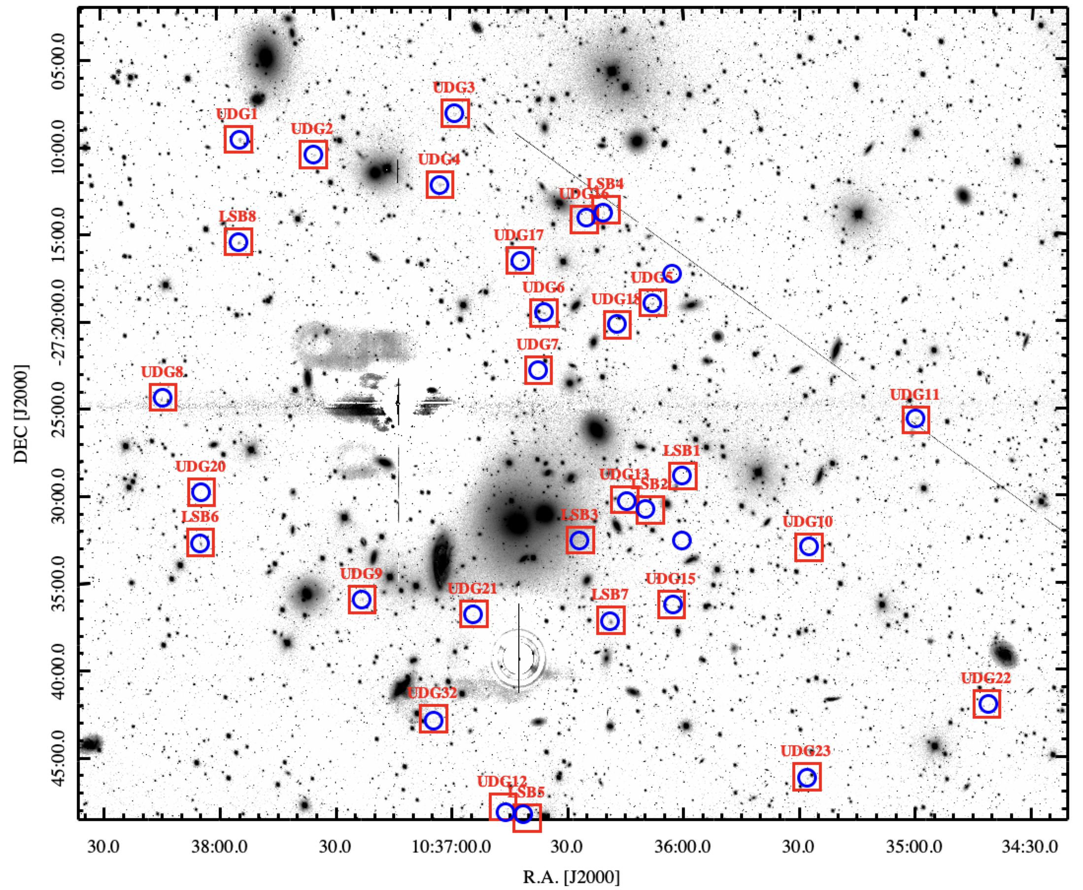
Figure 2: Optical $g$-band mosaic from VST of the Hydra I cluster ($56.7\arcmin\times 46.55$ ′$\sim 0.8\times 0.7$ Mpc). North is up and East to the left. The two bright stars, close to the cluster core, where modelled and subtracted from the image, as explained in Iodice et al. (2020). The 32 new UDGs and LSB galaxies detected by Iodice et al. (2020) and La Marca et al. (2022a) are marked as blue circles. Red boxes show the LEWIS sample presented in this work and listed in Table 1.

3 Observations and data reduction

The LEWIS observations are carried out with the MUSE integral-field spectrograph, mounted on the Yepun Unit Telescope 4 at the ESO Very Large Telescope in Chile. MUSE is used in Wide Field Mode without adaptive optics, providing a field of view (FoV) of 1$\times$1 arcmin², with a spatial sampling of 0.2$\times$0.2 arcsec². The nominal wavelength range of MUSE is from 4800 to 9300 Å with a spectral resolution (FWHM) that varies from 2.74 Å (69 km/s) at 5000 Å to 2.54 Å (46 km/s) at 7000 Å (Bacon et al., 2017).

Observations started in December 2021 during ESO period P108, and continued in periods P109 and P110. They are acquired in Service Mode, under dark and clear conditions. In the first two observing periods (P108 and P109) we gave priority to those UDGs that are fully consistent with the empirical classification proposed by van Dokkum et al. (2015), i.e. $R_{\rm e}\geq 1.5$ kpc and $\mu_{0,g}\geq 24$ mag/arcsec², having also photometrically detected GC candidates. Observations scheduled in P108 and P109 have been completed. The data acquisition for P110 targets, which mostly are LSB galaxies not classified as UDGs, is ongoing, with a completion of $\sim$20% in May 2023. In each run, and for each target, observations are executed in two steps. Shallower data are acquired to confirm the redshift first, and, for the confirmed cluster members, we obtained longer exposures to reach the depth required for our scientific purposes.

Since galaxies in the LEWIS sample span a wide range of effective surface brightness $25\leq\mu_{\rm e}\leq 27$ mag/arcsec², the total integration time adopted for each target was set by a required limiting magnitude $\mu_{\rm lim}=\mu_{\rm e}$ and a minimum SNR$=$7 in a spectral bin ($=2.51$Å) of 2$\times$2 pixels for the brighter targets and 5$\times$5 pixels for the fainter targets. Given that, the total integration times range from 2 hours for galaxies with $\mu_{\rm e}\simeq 25$ mag/arcsec² up to $\sim$6 hours for targets with $\mu_{\rm e}\simeq 27$ mag/arcsec². The total integration time for each target and the status of the data acquisition are reported in Table 1. Between single exposures we applied a dither of 0.3 to 1.3 arcseconds and a rotation by $90^{\circ}$, in order to minimise the signature of the 24 MUSE slices on the field of view.

3.1 Data reduction

Data are initially reduced with the MUSE pipeline version 2.8.5 (Weilbacher et al., 2016, 2020), under the ESOREFLEX environment (Freudling et al., 2013). The main steps include bias and overscan subtraction, flat fielding correction, wavelength calibration, determination of the line spread function, and illumination correction. Since all LEWIS targets are less extended than the MUSE FoV (see also Fig. 3), the sky has been evaluated directly on the science frames, as described in the following section. The flux calibration was obtained using spectro-photometric standard stars observed as part of the MUSE calibration plan. For each galaxy of the sample, the single exposures were aligned using reference stars and then combined to produce a first version of a stacked MUSE cube. In this first pipeline reduction, some of the default pipeline parameters for the sky subtraction and alignment for stacking were optimised.

3.2 Sky subtraction

After running the standard MUSE data reduction workflow, we used the resulting data products to obtain the final data cube with an improved sky subtraction, adapting the workflow described in Zoutendijk et al. (2020). The method and tools described below have been applied to one UDG of the sample, UDG11, chosen as a test case (see also Sec. 5). We used the reconstructed $r$-band image from the first version of the stacked MUSE cube to create an object mask. Objects were detected on the background-subtracted and Gaussian kernel convolved $r$-band image with the photutils software (Bradley et al., 2020). The resulting object mask was dilated by a factor of two and covers all visually detected foreground and background objects in the $r$-band image. To also cover the faint outskirts of the UDG that remained unmasked by the automatic object detection, we manually added an ellipse covering the central $1\;R_{\rm e}$ of UDG 11 ($R_{\rm e}=1.66\,\mathrm{kpc}$, ellipticity $\epsilon=0.3$, position angle P.A.$=144\degr$; Iodice et al., 2020).

We then ran ESOREFLEX again with the following modifications to the standard workflow. As we now used custom sky masks, we increased the fraction of pixels considered as the sky to SkyFr_2=0.75. Masking any non-sky objects in the sky also allowed us to use the autocalibration routines and we thus set autocalib=deepfield. The autocalibration method was originally developed for the MUSE deep field and uses the sky background to estimate correction factors for each slice in several wavelength bins after the rejection of outliers (Weilbacher et al., 2020), removing the spatial structure from MUSE exposures that remained after flat fielding. We also applied multiplicative flux calibration to each exposure before exposure combination, accounting for varying sky backgrounds. After applying these factors to the pixtables of the individual exposures, we combined them with the standard ESOREFLEX workflow.

Additional cleaning of the residual sky contamination was performed on the final stacked datacube, using the Zurich Atmospheric Purge algorithm (ZAP; Soto et al., 2016). ZAP was run within the ESOREFLEX environment, where a dedicated workflow is available within the MUSE pipeline. We parsed the custom sky mask to the workflow and tested different parameter combinations to obtain the optimum sky subtraction results. The reconstructed images of the final sky-subtracted data cube for UDG11, obtained with the standard prescriptions for the sky-subtraction and with the improved method described above, are shown in Fig. 3. The reconstructed images are displayed with the same intensity levels, which emphasises the improvement in the background level residual noise in our adopted “improved data reduction” (see top left panel of Fig. 3), with respect to the cube reduced with the standard sky-subtraction technique (top right panel of Fig. 3).

4 Cluster membership

The first goal of the LEWIS project is to confirm the cluster membership of all targets in the sample. To this aim, for each galaxy, we have derived the systemic velocity ($V_{\rm sys}$) by fitting the stacked spectrum inside $1R_{\rm e}$ with the Penalised Pixel-Fitting code (pPXF; Cappellari, 2017), using the MUSE rest-frame wavelength range between 4800 and 7000 Å. During this step, the region of the spectrum at longer wavelengths is excluded, since they are strongly affected by residuals from the sky line subtraction. Before obtaining the stacked spectrum, we used the MUSE reconstructed image to mask all the background and foreground bright sources. In addition, in the stacked spectrum are also masked all those wavelength regions with strong sky residuals. The MUSE reconstructed images and the stacked spectra, for all so far observed LEWIS galaxies, are shown in the Appendix A.

We have used the E-MILES single stellar population (SSP) models (Vazdekis et al., 2012, 2015) as spectral templates. They have a spectral resolution of FWHM $=2.51$ Å (Falcón-Barroso et al., 2011) and cover a large range in age (from 30 Myr to 14 Gyr) and total metallicity ($-2.27\leq$ [$M$/H] $\leq 0.4$ dex). The error estimate for each value of $V_{\rm sys}$ corresponds to the formal error provided by pPXF. The $V_{\rm sys}$ value for each of the observed galaxies is reported in Table 1.

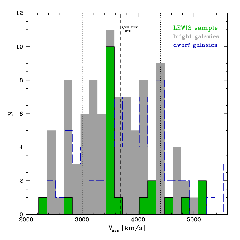
Figure 4: Velocity distribution of the galaxies in the LEWIS sample (green histogram). The distribution of velocities for the bright cluster members ($m_{B}<16$ mag) and for the dwarf galaxy population in the Hydra I cluster are shown with the grey and long-dashed blue histograms, respectively, from the catalogue by Christlein & Zabludoff (2003). The vertical dashed line marks the cluster mean velocity of $3683\pm 46$ km/s. The vertical dotted lines correspond to the average velocity dispersion of the cluster members $\sim 700$ km/s (Lima-Dias et al., 2021).

The distribution of $V_{\rm sys}$ values is plotted in Fig. 4. It ranges from 2317 km/s to 5198 km/s, with a peak value around $\sim 3500$ km/s, which coincides with the peak of the velocity distribution for the Hydra I bright ($m_{B}\leq 16$ mag) cluster members and dwarf galaxy population. The mean cluster velocity, $V_{\rm sys}=3683\pm 46$ km/s (Christlein & Zabludoff, 2003), and its velocity dispersion, $\sigma_{\rm cluster}\sim 700$ km/s (Lima-Dias et al., 2021), can be used to determine the membership of our targets: 14 of the 20 galaxies with the measured velocities are cluster members because they are found to have their velocity within the cluster velocity dispersion ($3438\leq V_{\rm sys}\leq 4302$ km/s). Since the cluster is quite isolated in the recession velocity space between 2000 and 5000 km/s (Richter et al., 1982; Richter, 1987), and the velocity distribution of its galaxy members is broad, the three galaxies with velocities inside $2\sigma_{\rm cluster}$ are also likely cluster members (UDG4, UDG8 and UDG12, see Table 1).The three remaining galaxies, UDG22 with $V_{\rm sys}=5198\pm 5$ km/s, LSB6 with $V_{\rm sys}=5193\pm 5$ km/s, and LSB8 with $V_{\rm sys}=2718\pm 5$ km/s, could be background or foreground galaxies.

In the photometric work of Iodice et al. (2020) and La Marca et al. (2022a), to discriminate UDGs from normal dwarfs LSB galaxies via their physical sizes, we assumed that all newly detected galaxies are at the distance of the Hydra I cluster (i.e. 51 Mpc). Now, having confirmed the cluster membership of most UDGs and LSB galaxies with our LEWIS spectroscopy, we stick to the fixed distance for deriving their effective radii and confirming their morphological classification, as already published in our previous papers (see also Table 1). We are aware that the Hydra I cluster might have a physical depth of a few Mpc, and thus some of the UDGs might be located in front or back of the cluster, resulting in size differences of $\pm 4$% for a relative distance of 2 Mpc with respect to Hydra I.

For the three outliers in the redshift distribution, we have used the Hubble law, assuming H₀=70 km/s/Mpc, to derive the Hubble flow distance based on the measured $V_{\rm sys}$. For UDG22 and LSB6, we obtained a distance of 74 Mpc and the new values for their effective radius are $R_{\rm e}=5.22$ kpc and $R_{\rm e}=5.80$ kpc, respectively. For LSB8, which has a lower $V_{\rm sys}$, $R_{\rm e}=1.12$ kpc. Therefore, UDG22 and LSB6 turn out to be more diffuse and fainter, if they would be a UDG and a LSB in the background of Hydra I cluster. LSB8 is smaller and, according to its central surface brightness $\mu_{0,g}=23.20$ mag/arcsec², it can be classified as a foreground dwarf galaxy.

5 Data quality and preliminary results: UDG11 as test case

This section describes the analysis of the MUSE data for one of the sample galaxies, UDG11, to assess the data quality. UDG11 has been chosen as a test case since it is one of the faintest and most diffuse galaxies in the sample, with a comparably large number of photometrically detected GC candidates (see Table 1), for which we obtained all the requested data at the desired depth. With this target, we customize and test the data reduction process as well as analysis tools and methods that will later be applied to the entire LEWIS sample. In the following sections, we describe the analysis of the MUSE cube for UDG11 to derive the i) line-of-sight velocity distribution LOSVD, ii) stellar population properties, and iii) systemic velocities of the GC candidates.

UDG11 is located on the west side of the cluster (see Fig. 2). The structural properties for this galaxy, based on deep images, were published by Iodice et al. (2020). In detail, UDG11 has an absolute magnitude $M_{r}=-14.75$ mag in the $r$ band and a stellar mass $M_{\star}=0.63\times 10^{8}$ M_⊙. The structural parameters derived from the 1D fit of the azimuthally-averaged surface brightness profiles, in the $g$ band, are $\mu_{0,g}=24.36\pm 0.13$ mag/arcsec² and $R_{\rm e}=1.66\pm 0.12$ kpc. The integrated colour is $g-r=0.43\pm 0.11$ mag. Based on the colour selection and shape, the estimated total number of GCs in this galaxy is $N_{\rm GC}=7\pm 3$ (see Iodice et al., 2020, and Table 1).

The MUSE cube obtained for UDG11 has a total integration time of 6.10 hours. The MUSE reconstructed images (from the whole wavelength range), resulting from the standard data reduction and improved procedure (see Sec. 3.2), are shown in Fig. 3. In the lower panels we compare, after arbitrarily re-scaling, the azimuthally-averaged surface brightness profiles from the MUSE reconstructed images with that of the optical VST image in the $g$ band. This illustrates that with the MUSE data for UDG11 we are able to map the integrated light down to $\mu_{g}\sim 28$ mag/arcsec² and out to $\sim$2$R_{\rm e}$, suggesting also that a satisfactory level of sky subtraction has been achieved. With the improved data reduction the residual patterns of the MUSE slices are well removed, even if the continuum appears slightly over-subtracted when compared to photometric profiles (Fig. 3).

From the MUSE cube obtained with the improved data reduction, and used for the analysis described in this paper, we have extracted the stacked spectrum inside a circular area with a radius $R=1R_{\rm e}$, where all bright sources (background galaxies and foreground stars) are masked. This is shown in Fig. 5. It is worth noting that the SNR per spaxel of the stacked spectrum from this cube is SNR=16, which is higher than the SNR=12.6 we computed for the spectrum from the standard data reduction. In addition, by masking the wavelength regions affected by the sky-lines residuals, the SNR increases to 20.

In this spectrum, we can clearly identify the absorption features of the most relevant lines, as H$\beta$, Mgb, H$\alpha$ and the CaT (see also lower boxes in Fig. 5). On the other hand, we do not detect emission lines, suggesting that this galaxy is devoid of ionised gas.

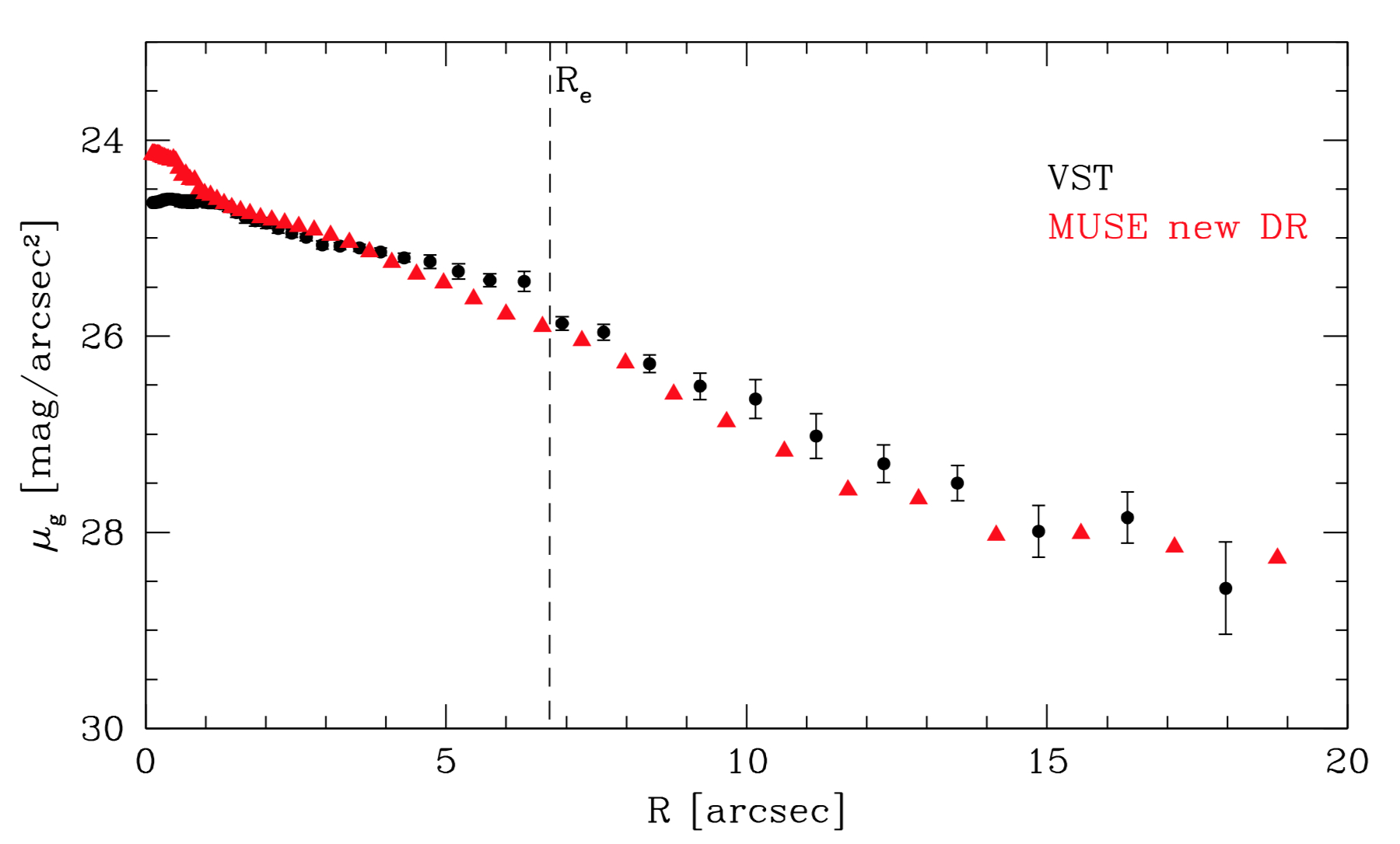
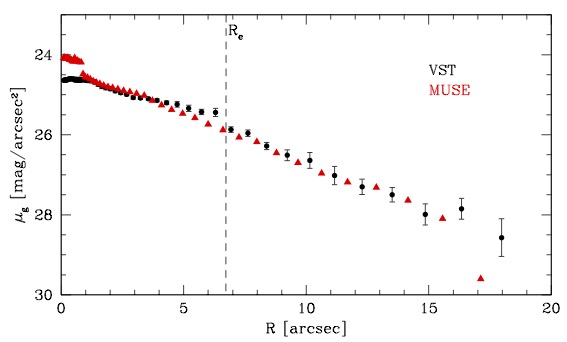
Figure 3: MUSE reconstructed image of UDG11. Top panels - reconstructed images obtained by improving the sky subtraction (left panel), as described in Sec. 3.2, and with the standard prescriptions for the data reduction (right panel). On the left panel, the dashed ellipse marks the isophote at $1R_{\rm e}$. The confirmed GCs are marked with the blue numbered boxes, see also Table 3. GCs 1 and 3 have radial velocities consistent with UDG11, while GCs 2 and 4 have radial velocities inconsistent with UDG11 but still consistent with the Hydra I cluster. The photometrically pre-selected GC candidates from Iodice et al. (2020) are marked with black circles. Four of them were found to be emission line galaxies, and for the other one it was not possible to retrieve the $V_{\rm sys}$ due to the low SNR (see Sec. 5.5 for details). Bottom panels - Azimuthally averaged surface brightness distribution derived from the MUSE reconstructed image (red triangles) compared with the same profile derived from the VST optical $g$-band image (black circles), obtained by improving the sky subtraction (left panel), and with the standard prescriptions for the data reduction (right panel). In both panels, the difference between VST and MUSE surface brightness profiles inside $\sim$1 arcsec is due to the seeing-limited observations of the optical VST images.

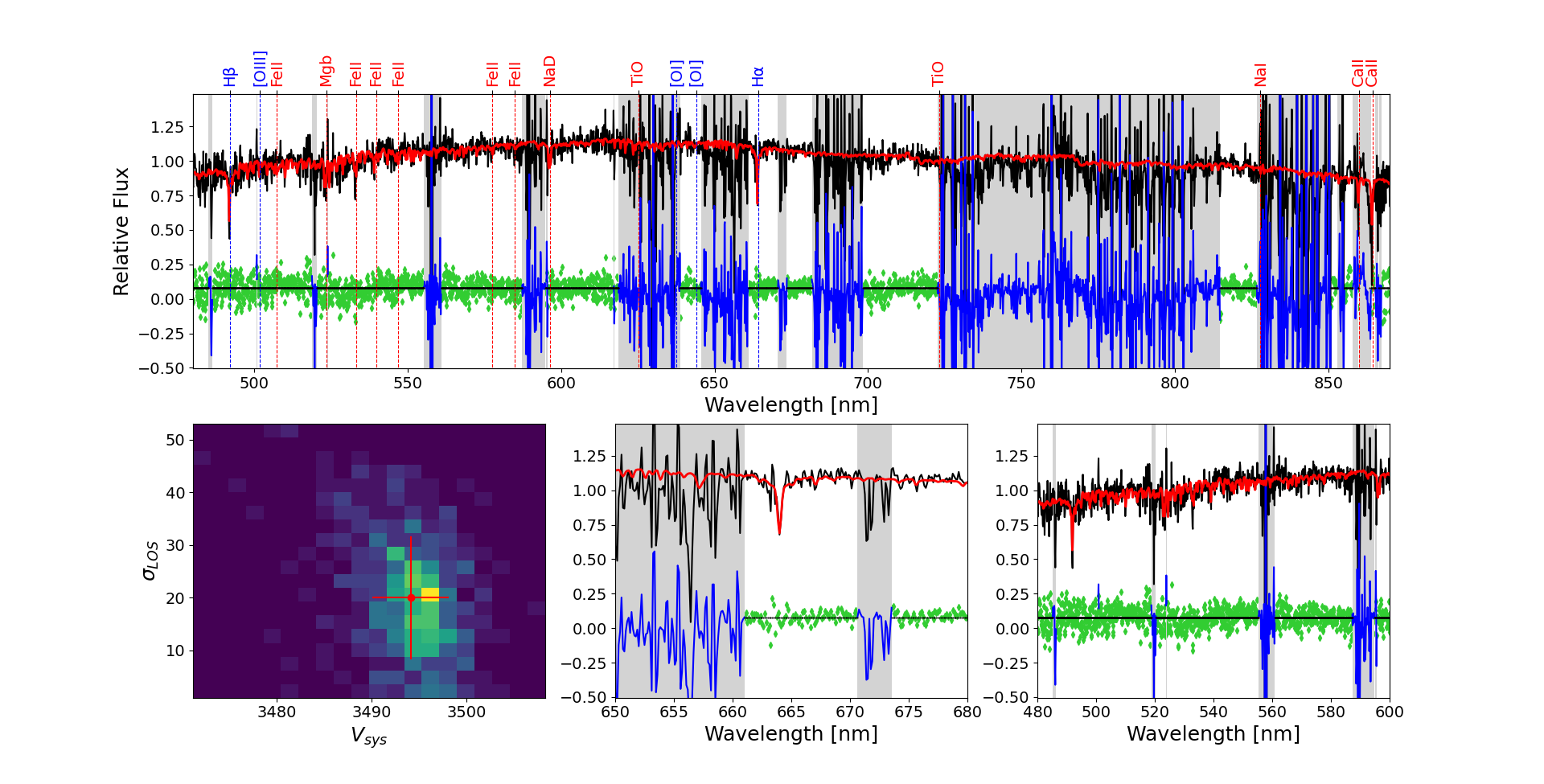
Figure 5: Restframe stacked MUSE spectrum (black solid line) for UDG11 derived inside $1R_{\rm e}$. The main absorption features are marked as dashed red (absorption features) and blue lines (absorption features, but potentially also in emission) and labels. The red solid line represents the best fit obtained with pPXF. Green points are the residuals between the observed spectrum and its best fit. The grey areas are the masked regions of the spectra, excluded from the fit. Bottom (right and middle) panels show the enlarged regions around the main fitted absorption features of the top-row fit in the optical wavelength range $4800-7000$ Å. The lower-left panel shows the grid of values for the line-of-sight velocity ($V_{\rm LOS}$) and velocity dispersion ($\sigma_{\rm LOS}$) derived from the Monte Carlo simulations (see text for details).

5.1 Stellar kinematics

The stellar kinematics of UDG11 have been derived by using the pPXF code. Specifically, we extract the LOSVD, which is parametrised by the line-of-sight (LOS) velocity $V$, velocity dispersion $\sigma$, and Gauss-Hermite moments $h_{3}$ and $h_{4}$ (Gerhard, 1993; van der Marel & Franx, 1993). We have used the E-MILES stellar library (Vazdekis et al., 2016) with single stellar population (SSP) models as spectral templates. These models have a spectral resolution comparable to the average of the MUSE spectra, i.e. $\sim$2.5 Å (see Sec. 3) which makes them suitable for our purposes. For all models, we have assumed a Kroupa IMF (Kroupa, 2001).

To assess the effectiveness of the MUSE cube and identify any potential constraints in measuring stellar kinematics caused by the low-surface brightness levels of these galaxies, we examined the entire MUSE rest-frame wavelength range, from 4800 to 9000 Å, as well as a restricted range, from 4800 to 7000 Å, which is less susceptible to the residual effects of sky line subtraction.

Since a reliable extraction of the higher-order Gauss-Hermite moments requires a relatively high SNR (e.g. Gadotti & de Souza, 2005, see also Fig. 7 of this study for exact estimations), for UDG11 we have derived only the first two moments of the LOSVD, i.e. $V$ and $\sigma$. These quantities have been estimated by running pPXF to fit the 1D stacked spectrum inside $1R_{\rm e}$. On the full MUSE rest-frame wavelength range between 4800 and 9000 Å, the best fit was obtained by allowing high-order multiplicative and additive Legendre polynomials of degree 10. Including additive polynomials allows to correct for differences in the flux calibration and overcome the limitations of the stellar library, whereas multiplicative polynomials directly alleviate imperfections in the spectral calibration affecting the continuum shape. Results are shown in Fig. 5. A similar approach was already used for the UDG NGC1052-DF2 by Emsellem et al. (2019) to estimate the stellar kinematics from MUSE data. The mean LOS velocity (which we adopted as systemic velocity) and velocity dispersion of UDG11 are $V_{\rm sys}=3507\pm 3$ km/s and $\langle\sigma\rangle_{\rm e}=20\pm 8$ km/s, respectively. Restricting the fit to the range 4800$-$7000 Å, the best fit provides $V_{\rm sys}=3509\pm 3$ km/s and $\langle\sigma\rangle_{\rm e}=20\pm 10$ km/s, being consistent with the former values.

The error estimates on $V_{\rm sys}$ and $\langle\sigma\rangle_{\rm e}$ are obtained by performing Monte Carlo simulations (e.g. Cappellari & Emsellem, 2004; Wegner et al., 2012). This procedure is described in Appendix B.

The stacked spectrum for UDG11 shows prominent absorption CaT lines (see Fig. 6). These lines are the strongest features in the stellar continuum for a large variety of stellar types (Cenarro et al., 2001), in addition to being at the MUSE wavelength region with better resolution (Bacon et al., 2017), they are particularly suitable to extract the stellar kinematics. We run pPXF on the wavelength region restricted to the rest-frame interval 8475$-$8690 Å. To fit exclusively the CaT region, we used the CaT templates by Cenarro et al. (2001). Given that the spectral resolution of these templates is $\sim$1.5 Å, they have been convolved to the resolution of the MUSE spectra in this range ($\sim$2.5 Å). The best fit, shown in Fig. 6, has been obtained with multiplicative and additive Legendre polynomials of degree 7, and by masking the reddest CaT lines, which is strongly affected by a residual of the sky lines. We obtain $V_{\rm sys}=3501\pm 5$ km/s and $\langle\sigma\rangle_{\rm e}=16\pm 12$ km/s. These values are consistent with the previous estimates, provided above, even if $\langle\sigma\rangle_{\rm e}$ has a larger error. All quantities, computed with the three different methods, are reported in Tab. 2.

5.2 Tests on the velocity dispersion measurements

By fitting the stacked spectrum inside 1$R_{\rm e}$, we have derived a very low value for $\langle\sigma\rangle_{\rm e}\sim 20$ km/s, less than the MUSE spectral resolution (see Sec. 3). As stated in the previous section, the fit has been performed by using the latest version of the pPXF code, developed by Cappellari (2017). The author proved that, for spectra with high SNR (SNR ¿ 3000 per spectral element), the full spectrum fitting provides reliable kinematics at any velocity dispersion, even below the instrumental resolution of MUSE.

Using the SAMI integral-field spectrograph to study the dwarf galaxies in the Fornax clusters, Eftekhari et al. (2022) proved that a velocity dispersion of $\sim 0.4$ the instrumental resolution can be measured, at SNR=15, with a $\sim 20-30$% of accuracy.

The LEWIS data are in the low-surface brightness regime, therefore, the main issue is the SNR of the spectra. Given that, we have performed several tests to check which is the minimum SNR needed for the data to retrieve a reliable value of $\sigma_{\rm LOS}$. We simulated mock spectra based on the E-MILES models, with different SNR ranging from 5 to 120 by introducing Poissonian noise. A full description of this test is reported in Appendix D.1. We found that, from spectra with SNR $\sim 15-20$ (comparable to that of the stacked spectrum of UDG11), we can retrieve velocity dispersion as low as $\sigma_{\rm LOS}\sim 10$ km/s with an uncertainty of 10 km/s. Results are shown in Fig. 7. Similar tests were performed by Eftekhari et al. (2022), and we found consistent results.

In conclusion, our tests demonstrate that we need a minimum SNR per spaxel of 10 for an unbiased velocity determination. Given that the stacked spectrum of UDG11, has SNR=16, the best-fit value for its velocity dispersion is $\langle\sigma\rangle_{\rm e}=20\pm 8$ km/s. This might be considered an upper limit, because we cannot exclude lower values.

In addition to the tests described above, we have performed a totally independent check of what is the expected value of the velocity dispersion for UDG11. By adopting the scaling relation derived by Zaritsky & Behroozi (2023), where the total mass-to-light ratio $\Gamma_{\rm e}$ derived inside $R_{\rm e}$ ($\Gamma_{\rm e}$) is a function of the velocity dispersion and the effective luminosity $I_{\rm e}$, we derived $\sigma=19.97$ km/s. In this relation, we have used $L_{\rm e}=3.35\times 10^{7}$ L_⊙, derived by Iodice et al. (2020), and we have assumed a total $M/L=10$, constant with radius, typical for dwarf galaxies of luminosity comparable to UDG11 (e.g. Battaglia & Nipoti, 2022). The resulting value of the velocity dispersion is fully consistent with the estimate obtained by fitting the MUSE cube. Therefore, even considering the limits of the data described above, we conclude that the derived estimate of the velocity dispersion for UDG11 is very close to the expected value for this galaxy.

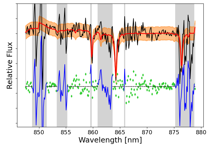
Figure 6: Stacked MUSE spectrum for UDG11 in the CaT region, inside $1R_{\rm e}$. The red solid line represents the best fit obtained with pPXF. Green points are the residuals between the observed spectrum and its best fit. The grey areas are the masked regions of the spectrum, excluded from the fit. The orange region corresponds to the standard deviation of the best fit across all the $\sim 1400$ iterations.

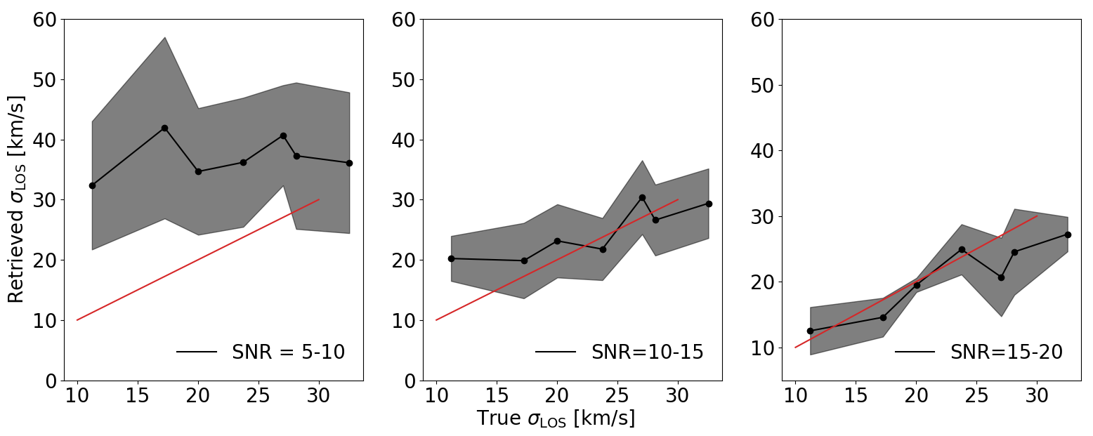
Figure 7: Results of simulations testing the ability of our pipeline to successfully recover a velocity dispersion of different values at low signal-to-noise (per pixel) levels, from SNR=5-10 (left panel), SNR=10-15 (middle panel), up to SNR=15-20 (right panel). Shaded areas correspond to the standard deviation of the measured values at every SNR. The red solid line corresponds to the output values equal to the input ones (unity line). In this experiment, the error is dominated by Poisson noise and no systematic sources of uncertainties have been considered. See Appendix D.1 for details.

5.3 Spatially-resolved stellar kinematics maps

The 2D map of the stellar kinematics is derived by using the modular Galaxy IFU Spectroscopy Tool (GIST) pipeline for the analysis of IF spectroscopic data, developed by Bittner et al. (2019). Using GIST, we spatially binned the datacube spaxels with the adaptive algorithm by Cappellari & Copin (2003) based on Voronoi tessellation. Since the average SNR of the stacked spectrum is $\sim$16, as binning threshold we adopted SNR$=$10 (Fig. 8, left panel). The fit was restricted to the optical wavelength range $4800-6800$ Å to avoid the region of the CaT, which is affected by the sky lines residuals, particularly in the galaxy outskirts. As starting guesses, we have used the same “set-up” of the best fit of the 1D stacked spectrum inside $1R_{\rm e}$. Therefore, we adopted the E-MILES stellar templates, additive polynomials of grade 10, and multiplicative polynomials of grade 10. In Figure 8 we show the map of the Voronoi bins, with the average signal-to-residual S/rN (left panel), the resulting 2D maps of the LOS velocity $V_{\rm LOS}$ (middle panel) and velocity dispersion $\sigma_{\rm LOS}$ (right panel). The SNR map shows that all bins close to the centre of the galaxy, corresponding to the brightest regions, have SNR$\geq 10$ per spaxel, which is the targeted threshold fixed for the Voronoi tessellation. In the galaxy outskirts, some bins have SNR$\leq 10$ per spaxel. This effect was discussed by Sarzi et al. (2018, see Fig.6 of that paper and references therein) for the MUSE cubes. They found that the quality of the Voronoi-binned spectra decreases with the surface brightness, where lower values of the SNR with respect to the formal threshold chosen for the Voronoi bins are found at the lowest surface brightness levels. This is due to the impact of the spatial correlations between adjacent bins at lower surface brightness levels.

From the 2D map of the LOS velocity dispersion (Figure 8, right panel), we extracted the effective velocity dispersion $\langle\sigma\rangle_{\rm e}$ by calculating the weighted mean of the values enclosed in an elliptical region with a semi-major axis equal to the effective radius and with axial ratio $q=1-\epsilon$, with ellipticity $\epsilon=0.3$. The associated error was estimated by calculating the standard error of the weighted mean. We found $\langle\sigma\rangle_{\rm e}=27\pm 8$ km/s, which is consistent within $1\sigma$ error with the different estimates derived from the 1D spectrum (Table 2). However, we have also tested more options where the degree of Legendre polynomials spans a larger range of values from 5 to 14. The resulting values of $\langle\sigma\rangle_{\rm e}$ are shown in Fig. 9. In order to be consistent with the stellar kinematics derived from the 1D stacked spectrum, we adopted the 2D maps obtained with the same multiplicative and additive polynomials (Fig. 8).

The 2D $V_{\rm LOS}$ map does not show a clear trend of rotation along any direction, the 2D $\sigma_{\rm LOS}$ map shows values ranging from $\sigma_{\rm LOS}\sim 10$ km/s to $\sigma_{\rm LOS}\sim 30$ km/s along the major axis, and larger values of $\sigma_{\rm LOS}\sim 40-50$ km/s along the minor axis of the galaxy. We checked the reliability of these measurements by inspecting the fit of the spectrum in each bin. We found that some bins in the outskirts have a SNR lower with respect to the adopted threshold for the Voronoi binning, therefore, in these bins, the values of $\sigma_{\rm LOS}$ are affected by a systematic overestimation, as addressed in Sec. 5.1 (see Fig. 7).

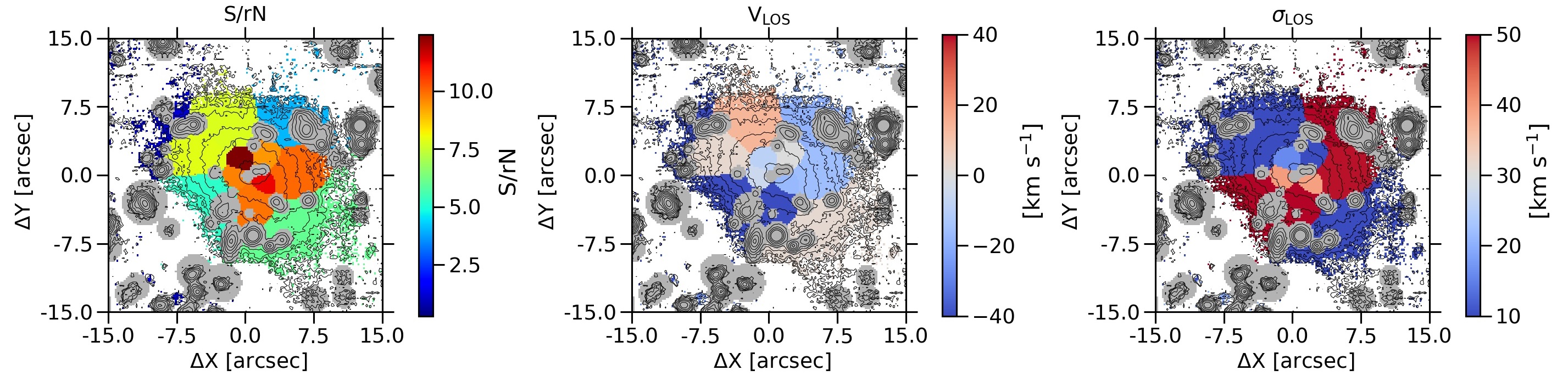
Figure 8: 2-dimensional kinematic maps of UDG11: signal-to-residual noise ratio S/rN (left), LOS velocity $V_{\rm LOS}$ (centre) and velocity dispersion $\sigma_{\rm LOS}$ (right) derived from a Voronoi binning with SNR=10. Contours correspond to the isophotes of the light distribution. Grey circles represent the adopted mask. The FoV is 30 $\times$ 30 arcsec and is oriented North up and East left.

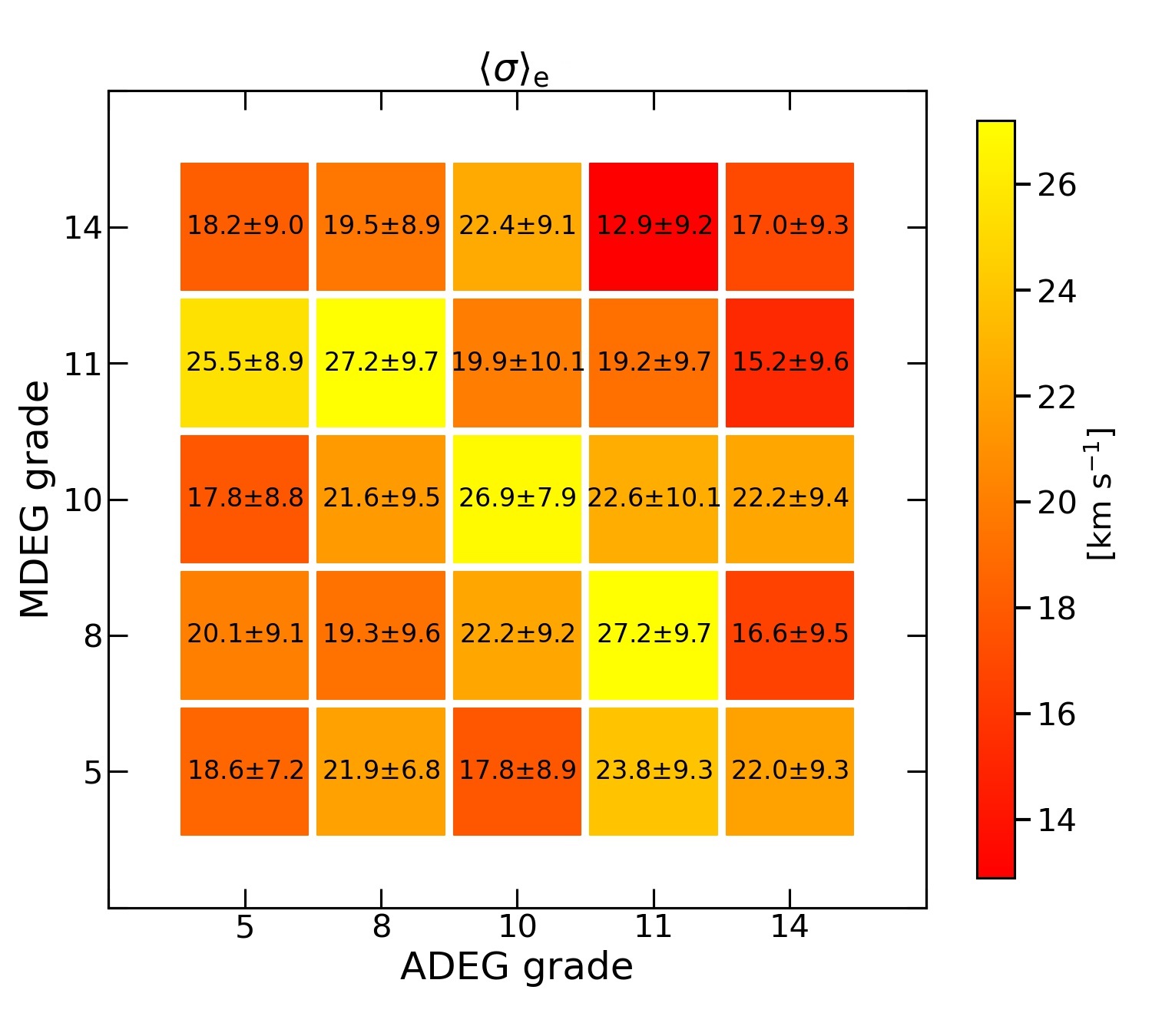
Figure 9: Values of the weighted mean of $\langle\sigma\rangle_{\rm e}$ derived from the fit of the Voronoi binned cube (with SNR=10 per spaxel) for different degrees of multiplicative and additive Legendre polynomials. Boxes are colour-coded according to the value of $\langle\sigma\rangle_{\rm e}$. See text for details.

5.4 Stellar populations

For UDG11, we have performed an additional pPXF run on the stacked spectrum inside $1R_{\rm e}$ in order to derive its mean age and total metallicity. We have fitted the full MUSE rest-frame wavelength range between 4800 and 9000 Å, using the E-MILES templates (Padova isochrones with Kroupa IMF; Girardi, L. et al., 2000). As first step, we have generated a reference fit, to be used also as a central setting for the generation of bootstrapped spectra and as reference for Monte Carlo iterations over various parameters (see Appendix B). This step involves the creation of a mask, flagging all noisy pixels and sky lines affecting the spectra (with a flux greater than three times the noise level). The process also includes setting polynomial degrees as shown in Sec. 5.1: we utilise the same framework as the 1D stacked spectrum, but with the exclusion of additive polynomials. In addition, we also fix our previously found 1D kinematic solutions to those from the stellar population fits, constraining in this way the velocity dispersion.

To construct the final solution, pPXF uses a technique called regularization, which allows the routine to preferentially select the smoothest solution among many (products of the well-known age-metallicity degeneracy; see e.g, Cappellari, 2017).

Over 700 iterations, the median age and metallicity which we obtained by fitting the whole MUSE wavelength range, are Age$=10\pm 1$ Gyr and [$M$/H]$=-1.17\pm 0.11$ dex, respectively. By fitting the stacked spectrum for one of the confirmed GCs (see Sec. 5.5), we obtained comparable age ($7.9\pm 1.5$ Gyr) and metallicity ([$M$/H]$=-0.7\pm 0.3$ dex). Results are plotted in Fig. 10 (left panel) and listed in Table 2.

As a self-consistency check, we take the E-MILES set of templates (BaSTI isochrones with the same Kroupa IMF) and compute the Lick H$\beta$ and [MgFe]’ indices of various templates in order to construct a reference grid. This computation is done with the latest version of pyphot without following the usual Lick indices convention (see e.g, Vazdekis et al., 2010) for the assumed FWHM. Instead, to avoid losing potentially useful information, we keep the resolution of the data intact, as it roughly matches the one of the templates used to construct the grid. To compute the errors on the Lick indices, we take Lick measurements for every best fit model from each converging pPXF iteration, and then use the 1$\sigma$ measurement on the Monte Carlo distribution to estimate the error. We find the Lick indices measurements to be fairly consistent (Lick H$\beta=2.54\pm 0.2$ and [MgFe]’ $=1.49\pm 0.1$) with the stellar population measurements of age and metallicity. Results are shown in Fig. 10 (right panel).

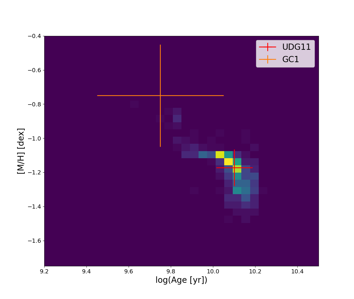
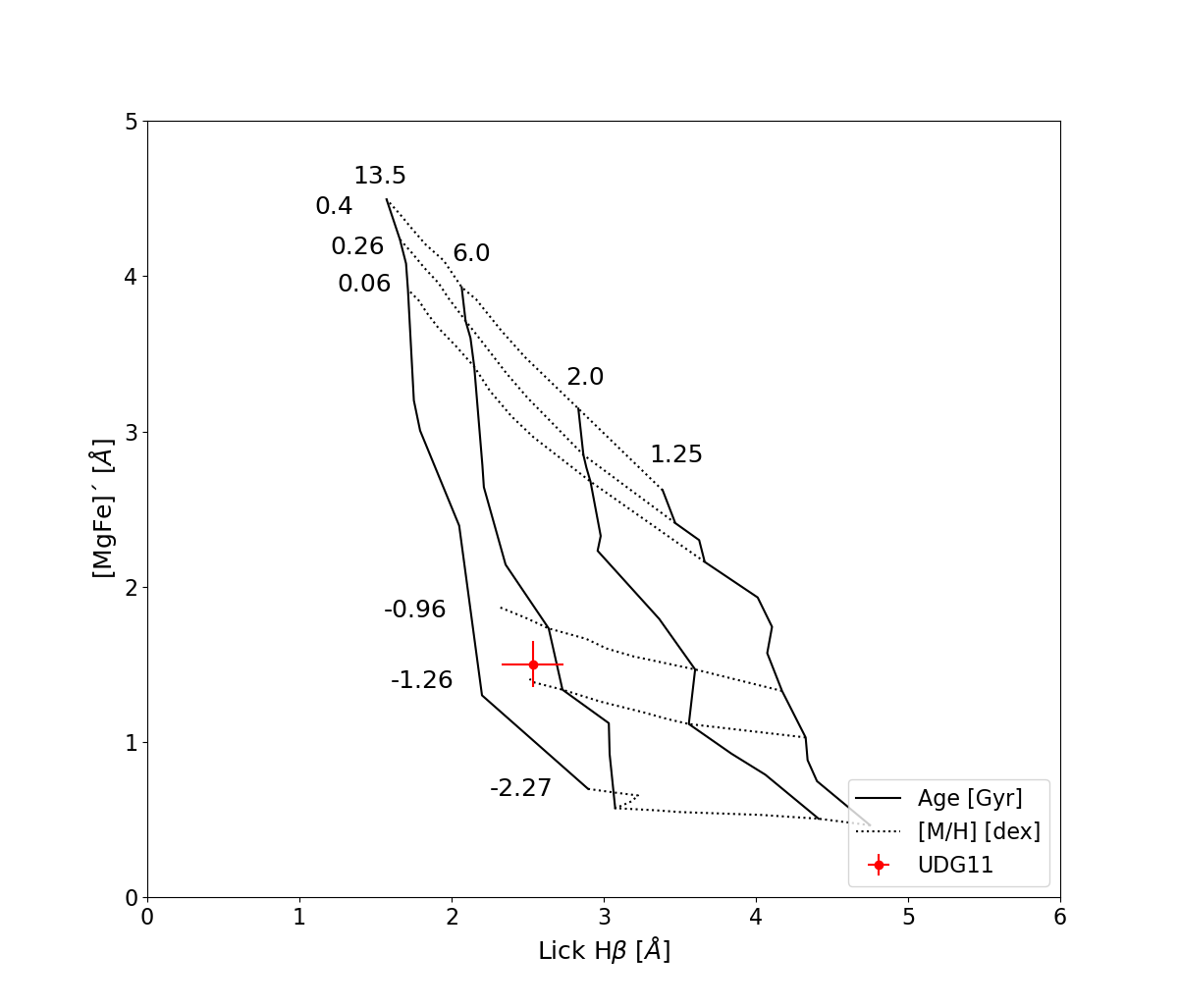
Figure 10: Mean age and metallicity for UDG11 derived from the stacked spectrum inside $1R_{\rm e}$. Left panel - Best fit derived using the pPXF code. The red cross corresponds to the values for age and metallicity (including errors) obtained by the best fit on the whole MUSE spectral range. The orange cross shows the average age and metallicity (including errors) for one of the confirmed GCs in UDG11 (see Sec. 5.5). Right panel - Lick indices measurements. Using the E-MILES BaSTI templates, we constructed the grid: vertical dashed lines denote models for the same age (left being the oldest), and horizontal dotted lines refer to model measurements for spectra with the same metallicity (with the most metal poor ones located at the lower part).

Table 2: Stellar kinematics, age and metallicity derived for UDG11 from the LEWIS data.

Fit	$\lambda$ range	$V_{\rm sys}$	$\langle\sigma\rangle_{\rm e}$	[$M$/H]	Age
	[Å]	[km/s]	[km/s]	[dex]	[Gyr]
(1)	(2)	(3)	(4)	(5)	(6)
1D	4800-9000	3507$\pm$3	20$\pm$8	$-1.2\pm$0.1	10$\pm$1
1D	8475-8690	3501$\pm$5	16$\pm$12	–	–
2D	4800-7000	3532$\pm$43	27$\pm$8	–	–
GC1	4800-9000	3503$\pm$12	–	$-0.7\pm$0.3	9$\pm$2

5.5 Globular cluster population

From the UDG11 MUSE cube, we extracted and analysed the spectra of the photometrically pre-selected GC candidates from Iodice et al. (2020), as well as all other point-like sources within the luminosity range expected for GCs (see also Fig. 3). Where the signal-to-noise was sufficient, we measured the radial velocity to verify their kinematical association with the UDG.

We only considered the sources with SNR $\geq 2.5$ in the background subtracted spectrum, using an 8-pixel circular aperture. For lower SNR, the $V_{\rm sys}$ could not be reliably determined. This SNR limit corresponds to an apparent magnitude of $m_{g}\sim 25.5$ mag, about 0.5 mag brighter than the expected turn-over magnitude (TOM) of the GC luminosity function (GCLF) at the distance of the Hydra I cluster (Iodice et al., 2020).

For measuring the radial velocity of the candidate GCs, we used the SSP model spectra from the E-MILES library to fit each GC spectrum with pPXF. In this case, we used an IMF with a double power-law (bimodal) shape and a high mass slope of 1.30 (Vazdekis et al., 1996). We did not attempt to measure the intrinsic velocity dispersion of the candidate GCs, due to the low spectral resolution of MUSE and the limited SNR of the observed spectra (see also Fig. 7).

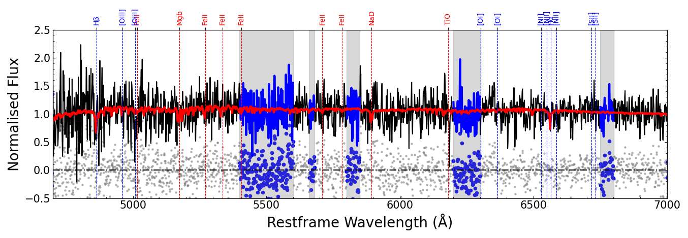
Figure 11: Stacked spectrum of GC3, with SNR $\sim$4.5 Å^-1. The original spectrum is shown in black, the pPXF fit in red. Regions with strong sky residual lines were masked from the fit (grey-shaded areas).

Figure 11 shows the spectrum of one GC in the field, and the corresponding pPXF fit as an example. The regions excluded from the spectrum are grey-shaded and correspond to the residual sky or telluric lines. Moreover, we excluded from the fit the wavelength region with $\lambda\geq 7000$Å because of the presence of strong sky residuals which made the identification of the CaT not feasible.

Also in this case, to get a reliable uncertainty on the estimate of $V_{\rm sys}$ we fitted the sources in a Monte Carlo technique approach (see Sec. 5.1). After the first fit using the original spectrum, we created 200 realizations with the same SNR of the original spectrum by perturbing the noise-free best-fit spectrum with random draws in each wavelength bin from the residual (best-fit subtracted from the original spectrum). The fit was then repeated and the LOS velocity was determined from the mean of the resulting distribution. The random uncertainty is given by the standard deviation assuming a Gaussian distribution. A detailed description of the method to study the GC population in UDGs, including UDG11, is the subject of a forthcoming paper by Mirabile et al. (in prep.).

We identified four point sources in the UDG11 cube with a $V_{\rm sys}$ velocity consistent with the Hydra I cluster. They are listed in Table 3 and marked in Figure 3. The projected position of GC1, GC2 and GC3 is within $2R_{\rm e}$ of UDG11, while GC4 is much more distant ($\sim 4R_{\rm e}$).

The radial velocity of GC1 and GC3 are 3503 $\pm 12$ km/s and 3460$\pm 21$ km/s, respectively. Compared to the systemic velocity of the UDG11, they are within $1\sigma$ and $\sim$2$\sigma$, respectively. We therefore consider that both GCs are associated to UDG11. Moreover, it’s worth noting that the velocity differences $\Delta V$ of GC1 and GC3, of $\Delta V\sim-4\pm 13$ km/s and $\Delta V\sim-47\pm 22$ km/s (see Table 3), respectively, are consistent with the stellar velocity dispersion obtained for UDG11 close to the centre ($\sigma_{\rm LOS}\sim 20$ km/s) and in the South-East region of the galaxy ($\sigma_{\rm LOS}\sim 20-40$ km/s), as shown in Fig. 8.

The velocity difference $\Delta V\geq 130$ km/s for GC2 and GC4 might suggest they are not gravitationally bound to UDG11, and, therefore, they might be considered as intra-cluster GCs. However, this result can only be confirmed once the DM content of this galaxy gets better constrained. To this aim, we calculated the escape velocity assuming a NFW halo profile (Miller et al., 2016), and we estimated the DM halo mass using the Burkert & Forbes (2020) relation. We found that, if the DM halo mass lies between 4 and $6\times 10^{10}$ M_⊙, the GCs with an escape velocity $\leq 200$ km/s can be considered as bound systems. Therefore, GC2 with $\Delta V\simeq 260$ km/s should be considered an intra-cluster GC, whereas all the other GCs could potentially be bound to the UDG11. Finally, the very central GC, GC1, might be a nuclear star cluster.

In summary, the preliminary analysis of the GC systems in UDG11 suggests that this galaxy has either two or three spectroscopically confirmed GCs that are bound to the host. By excluding GC1, as a potential nuclear star cluster and GC2 as an intra-cluster GC, with the remaining two spectroscopically confirmed GCs we can estimate the GC specific frequency ($S_{N}$) of UDG11. Our spectroscopic completeness limit is $m_{g}\sim 25.5$ mag ($m_{r}\sim 24.9$ mag), which is 0.5 brighter than the GCLF turnover magnitude of $m_{g}^{\rm TOM}$=26 mag (Iodice et al., 2020). Assuming a GCLF width of $\sigma_{\rm GCLF}$=1 mag (Villegas et al., 2010), our spectroscopic completeness limit thus corresponds to 34% of the GCLF. The incompleteness corrected total number of GCs then is 2/0.34=$5.9^{+2.2}_{-1.8}$, where the error range comes from the 68% confidence interval of a Poisson distribution centred on 3.9 (i.e. the number of 2 spectroscopically confirmed GCs has no errorbar, only the incompleteness correction of 3.9 has it). The absolute $V$-band magnitude of UDG11 is $M_{V,0}=-14.6\pm 0.1$ mag. Therfeore, we obtain $S_{N}=8.4^{+3.2}_{-2.7}$. This value of $S_{N}$ is consistent with the typical estimates for dwarf galaxies of similar luminosity (Georgiev et al., 2010; Lim et al., 2018). By including both GC1 and GC2, the value of $S_{N}$ would correspondingly change, but it is still consistent within the uncertainties with the values quoted above.

It is worth noting that none of the five photometrically pre-selected GC candidates from Iodice et al. (2020, see Fig. 3, black circles), can be confirmed as GC associated to UDG11: four of them exhibit emission lines typical of background galaxies and one has too low SNR for a reliable velocity measurements. From Iodice et al. (2020) the number of contaminants is $3.3\pm 0.8$ arcmin^-2, therefore, for a region of $5R_{\rm e}$ around the UDG11, we expect a number of contaminants equal to $3\pm 1$. Among the five photometrically pre-selected GCs, one would thus have expected about two spectroscopically confirmed GCs. This is indeed the case. We note that the majority of photometrically pre-selected candidates have not been confirmed, while the two newly detected GCs within the MUSE cube did not pass the narrow photo- and morpho-metric selections adopted for the VST dataset. This is not surprising, given the availability of only two photometric and very close optical bands. The preliminary results on other LEWIS targets reveal that UDG11 is rather peculiar in this respect. As an example, out of five photometric preselected GC candidates of UDG3, three are spectroscopically confirmed GCs, whereas the remaining two have too small SNR to provide useful constraints (further details will be presented in Mirabile et al., in prep.).

Table 3: Identified GCs in the UDG11.

GC	RA	DEC	$V_{\rm sys}$	$\Delta V$	$m_{r}$	SNR	Galactocentric Distance	Classification
	[deg]	[deg]	[km/s]	[km/s]	[mag]		[kpc]
(1)	(2)	(3)	(4)	(5)	(6)	(7)	(8)	(9)
1	158.7482	-27.427	3503$\pm$ 12	-4$\pm$ 13	24.57 $\pm$ 0.07	10.2	¡$R_{\rm e}$	GC/Nucleus
2	158.7477	-27.4280	3767$\pm$ 54	+260$\pm$ 54	24.05$\pm$ 0.07	5.8	¡$R_{\rm e}$	Intra-cluster GC?
3	158.7479	-27.4293	3460$\pm$ 21	-47$\pm$ 22	24.18$\pm$ 0.08	4.5	$<1-2R{\rm e}$	GC
4	158.7523	-27.4339	3640$\pm$ 33	+133$\pm$ 34	24.88 $\pm$ 0.03	2.7	$\sim 4R_{\rm e}$	Intra-cluster GC?

6 The structure of UDG11 from LEWIS data

In this section, we discuss the stellar kinematics, stellar populations and DM content of UDG11, as a result of the analysis of the MUSE cube presented in this paper. The main goal is to probe the ability of the LEWIS data to constrain these quantities, the relative uncertainties, and, therefore, the formation history of UDGs.

6.1 Stellar kinematics and populations of UDG11

In Table 2 we summarised the measurements of the stellar kinematics (i.e. systemic velocity and velocity dispersion) and the average age and metallicity, derived for UDG11 (see Sec. 5.1 and Sec. 5.4). Based on the fit of the 1D stacked spectrum inside $1R_{\rm e}$, these estimates suggest that the UDG11 has a very low velocity dispersion ($\langle\sigma\rangle_{\rm e}\sim 20$ km/s), it is old ($\sim 10$ Gyr) and metal-poor ([$M$/H]$\sim-1.2$ dex). The spatially-resolved map of the LOS velocity (see Fig. 8, central panel), does not reveal a significant velocity gradient or rotation along the photometric axes of the galaxy.

In Fig. 12 we show the histograms of the stellar mass, velocity dispersion, age and metallicity measured for UDGs in previous works. The observed values obtained for UDG11 in this paper are also reported for comparison. These plots suggest that the velocity dispersion estimated for UDG11 ($\sigma\sim 20$ km/s) fits into the broad range of $\sigma$ values for the majority of UDGs ($8\leq\sigma\leq 32$ km/s), which peaks at $\sigma\sim 20$ km/s (see top-right panel of Fig. 12). Based on the few measurements for the stellar population in UDGs, both age and metallicity span a wide range of values. On average, UDGs seem to be old ($7\leq$ Age $\leq 14$ Gyr) and metal-poor ($-1.8\leq[M$/H$]\leq-0.5$ dex). However, younger ages ($\sim 1$-4 Gyr) and sub-solar metallicity ([$M$/H]$\sim-0.1$ dex) are found for a few objects (see lower panels of Fig. 12). The age and metallicity estimated for UDG11 fit well with the typical values observed for old and metal-poor UDGs.

In Fig. 13 we show the relations between the velocity dispersion and metallicity as a function of the stellar mass for UDGs. In both panels, UDG11 has comparable values with other UDGs of similar stellar mass, taking into account the uncertainties on both measurements. As already pointed out by Gannon et al. (2021), in the $\sigma$-mass relation, the majority of UDGs, including UDG11, are found in the same region where other dwarf galaxies are located. However, some UDGs scatter to lower and higher $\sigma$ values compared to the tighter $\sigma$-mass relation of “normal” dwarf galaxies.

In the mass-metallicity plane, UDGs show a large scatter (see right panel of Fig. 13). Most UDGs, including UDG11, are consistent with the typical values for dwarf galaxies in the same range of masses (Kirby et al., 2013; Simon, 2019). Also in this case, lower ([$M$/H]$\leq-1.5$) and higher ([$M$/H]$\geq-1$) metallicity than the average are found. In particular, these estimates are also consistent with the observed age and metallicity derived for a large sample of dwarf galaxies (Heesters et al., 2023; Romero-Gómez et al., 2023), where ages and metallicities range from 5 to 14 Gyr, and 0 to -1.9 dex, respectively.

A detailed discussion on the formation history of UDG11 is out of the scope of this paper, which, instead, will be presented in the context of the full sample. However, we briefly comment below on how the LEWIS data can be used to address the structure and formation of UDGs in a cluster environment. According to Sales et al. (2020), at a given stellar mass, the T-UDGs show lower velocity dispersion and higher metallicity than the B-UDGs and normal dwarf galaxies. In addition, B-UDGs are found at larger cluster-centric distances ($\geq 0.5R_{200}$) than T-UDGs, whose spatial distribution peaks around the cluster core (see Fig.7 in Sales et al., 2020). The observed properties of UDG11, from the deep VST images and LEWIS data, are similar to those predicted for the B-UDGs. UDG11 is located on the west side of the cluster, at about $0.4R_{\rm vir}$, in the low-density region of dwarf galaxies (see La Marca et al., 2022a), and the measured velocity dispersion and metallicity are similar to those of dwarf galaxies (see Fig. 13).

6.2 Dark matter content of UDG11

We computed the dynamical mass of UDG11 using the mass estimator proposed by Wolf et al. (2010), where $M_{1/2}=4\times R_{\rm e}G^{-1}\langle\sigma\rangle_{\rm e}^{2}$. Using $\langle\sigma\rangle_{\rm e}=20\pm 8$ km/s, derived from the fit of the 1D stacked spectrum, we obtain $M_{1/2}=4.2\pm 0.8\times 10^{8}$ M_⊙. This is the dynamical mass inside half of the total luminosity. The absolute magnitude in the $V$ band for UDG11 is $M_{V,0}=-14.6\pm 0.7$ mag, therefore the total dynamical mass-to-light ratio is $M/L_{V}=2\times M_{1/2}/L_{V}\simeq 14$ M${}_{\odot}/$L_⊙.

UDG11 seems to have a total mass comparable to Local Group dwarfs of similar luminosity, which have a $M/L_{V}\sim 10-100$ (Battaglia & Nipoti, 2022). This suggests a dwarf-like DM halo for this UDG.

According to the stellar mass-halo mass relation derived down to the lowest stellar masses (Wang et al., 2021), which is comparable to the stellar mass of UDG11 ($M_{*}\sim 10^{8}$ M_⊙), the expected halo mass is M${}_{\rm h}\sim 10^{10}$ M_⊙. A similar value is also obtained by using the halo mass-stellar mass relation derived by Zaritsky & Behroozi (2023), where $M_{\rm h}=10^{10.35}\times[M_{*}/(10^{8}$ M${}_{\odot})]^{0.63}\simeq 1.7\times 10^{10}$ M_⊙.

Using the scaling relation between the halo mass and the total number of GCs, which is $\log[M_{\rm h}]=9.68+1.01\times\log[N_{\rm GC}]$ (Burkert & Forbes, 2020), and assuming that it is still valid in the low-mass regime, a consistent value of halo mass is found, $M_{\rm h}\sim 4\times 10^{10}$ M_⊙, where we adopt $N_{\rm GC}=5.9^{+2.2}_{-1.8}$ (see Sec. 5.5). However, it is worth noting here that this estimate for the halo mass is made under the assumption that the central GC1 is a nuclear star cluster, and that GC2 does not belong to UDG11. Including both GCs would result in a higher $S_{N}$ and halo mass, which would still be consistent within the uncertainties with the values quoted in Sec. 5.5.

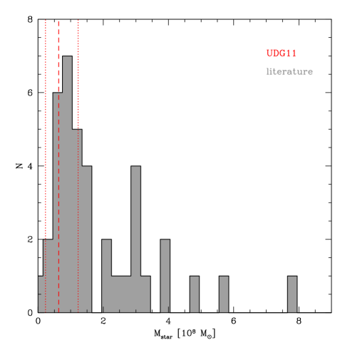
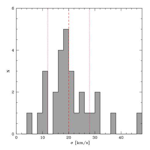
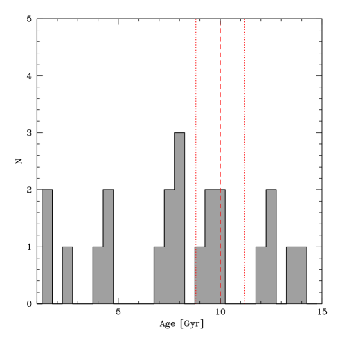
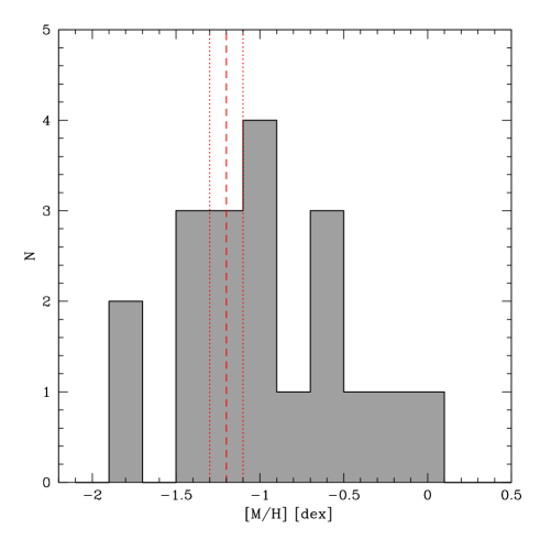
Figure 12: Stellar kinematics and stellar populations for UDGs from the literature compared with UDG11. Histograms (in grey) represent the stellar mass (top-left), velocity dispersion (top-right), age (bottom-left) and metallicity (bottom-right) for UDGs from previous works (Ruiz-Lara et al., 2018; Ferré-Mateu et al., 2018; Chilingarian et al., 2019; van Dokkum et al., 2019; Emsellem et al., 2019; Fensch et al., 2019; Gannon et al., 2021, 2023; Toloba et al., 2018; Martín-Navarro et al., 2019). In all panels, the average value derived for UDG11 and error estimates are marked with the vertical red dashed and dotted lines, respectively. Values are obtained from the fit of the stacked spectrum inside $1R_{\rm e}$, and listed in the first column of Table 2.

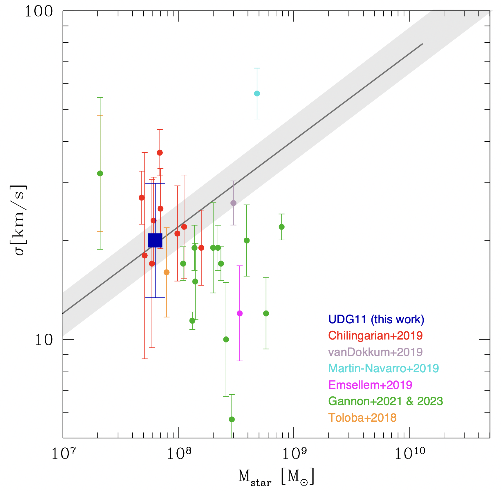
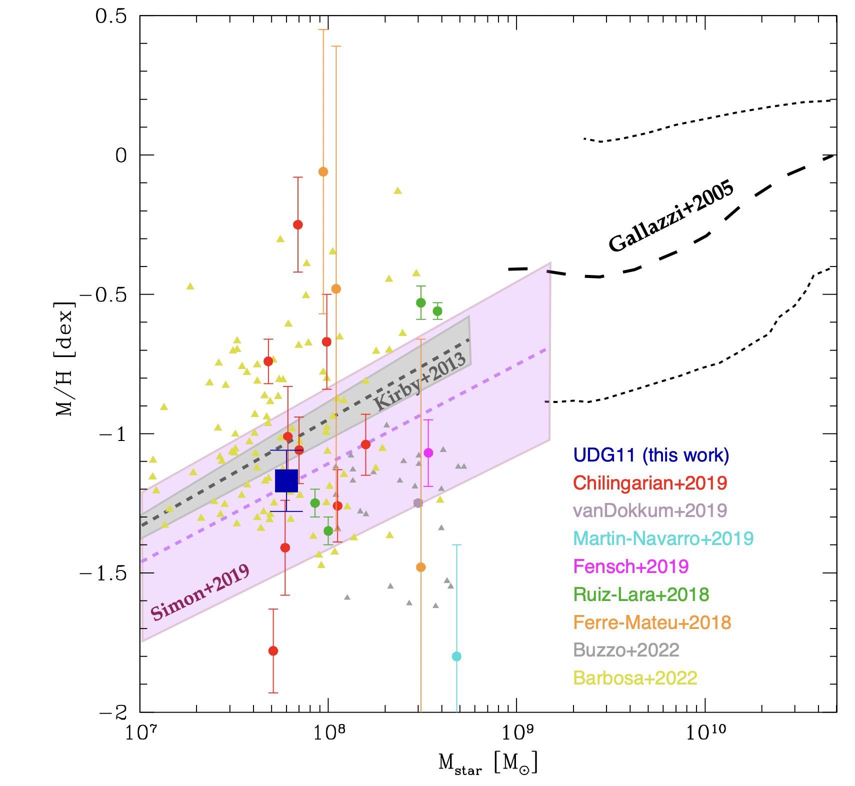
Figure 13: Velocity dispersion and metallicity as function of stellar mass for UDGs. Left panel - $\sigma$-mass relation for UDGs from the literature (coloured points) and UDG11 (blue square). The grey area corresponds to the observed baryonic Tully-Fisher relation (McGaugh, 2012), obtained by scaling the rotation velocity by $\sqrt{3}$. Right panel - Mass-metallicity relation from observations, including UDG11. The mass-metallicity relations found for dwarf galaxies by Kirby et al. (2013) and by Simon (2019) are marked in grey and purple regions, respectively. The average mass-metallicity relation for bright galaxies is marked by the black dashed line, and its range by the two dotted lines (Gallazzi et al., 2005). The metallicity derived by fitting the spectral energy distribution by Buzzo et al. (2022) and Barbosa et al. (2020) are marked with grey and yellow triangles, respectively. In both panels, data-points from Chilingarian et al. (2019) are UDG-like, since only two objects of the sample have $\mu_{0}\geq 24$ mag/arcsec² and $R_{\rm e}\geq 1.5$ kpc.

7 Summary and concluding remarks

In this paper, we have presented the LEWIS project. LEWIS is a large observing programme started in 2021 to obtain the first homogeneous integral-field spectroscopic survey of LSB galaxies, including UDGs, in the Hydra I cluster of galaxies, with MUSE at ESO-VLT. The LEWIS sample consists of 30 galaxies, 22 UDGs and 8 LSB dwarfs, with effective surface brightnesses in the range $25\leq\mu_{\rm e}\leq 27.5$ mag/arcsec² in the $g$ band (Table 1). The total integration time per target varies from 2 hours, for the brightest objects, up to 6 hours for the faintest ones.

With the LEWIS project we expect to constrain i) the fraction of baryonic versus DM content, ii) the star formation history, and iii) the GCs content by means of spectroscopic $S_{N}$, in all sample galaxies. Given the large variety of observed properties for UDGs (mainly based on deep images), and theoretical scenarios, which envisage various possibilities for the formation of this kind of galaxy, the main outcomes of this project are a notable boost to our knowledge of the UDG structure and formation.

LEWIS observations are still ongoing. In this paper we have presented the LEWIS sample and the measured redshift for the 20 targets (16 UDGs and 4 LSB dwarfs) observed so far. Fourteen of them have been confirmed as Hydra I cluster members, with systemic velocities ranging from 3483 km/s to 4302 km/s, which correspond to $\sim$1$\sigma$ from the cluster mean velocity ($V_{\rm sys}=3683\pm 46$ km/s, $\sigma_{\rm cluster}\sim 700$ km/s). Three galaxies of the sample have systemic velocities within $2\sigma_{\rm cluster}$, therefore they might be still considered as cluster members. Finally, the remaining three galaxies with larger or smaller systemic velocities could be considered as background or foreground galaxies, respectively.

To assess the quality of the LEWIS data, we have also described the data analysis that we adopt in this project, for one of the sample galaxies, UDG11, chosen as test case. UDG11 is located far from the cluster core, on the west side, at a distance of $\sim 0.4$ R_vir. It has an absolute $r-$band magnitude of $M_{r}=-14.75$ mag and a stellar mass of $0.63\times 10^{8}$ M_⊙. The MUSE data obtained for this target have a total integration time of 6.10 hours, which allowed us to obtain a SNR$\sim 16$ per spaxel, for the 1D stacked spectrum inside $1R_{\rm e}$. For this target, we have derived the stellar kinematics, constrained the average age and metallicity of the stellar populations, estimated the total number of spectroscopically confirmed GCs, and provided the dynamical mass. All the above quantities are compared with the available measurements for UDGs and dwarf galaxies in literature. Results are summarised below.

• By fitting the stacked spectrum inside $1R_{\rm e}$, on the full MUSE rest-frame wavelength range ($4800-9000$ Å), we obtained a velocity dispersion $\sigma=20\pm 8$ km/s, a metallicity [$M$/H]$=-1.17\pm 0.11$ dex and an age of $10\pm 1$ Gyr.

• The spatially resolved stellar kinematics, obtained from the Voronoi-binned spectra with SNR = 10, show that UDG11 does not show a significant gradient of $V_{\rm sys}$ and $\sigma_{\rm LOS}$ along major and minor photometric axes. The mean value of the velocity dispersion is $\langle\sigma\rangle_{\rm e}=27\pm 8$ km/s, which is consistent with the estimate from the fit of the stacked spectrum inside $1R_{\rm e}$.

• The absence of emission lines in the MUSE cube for UDG11 suggests that this galaxy lacks ionised gas.

• Four point sources in the UDG11 cube have radial velocities consistent with the Hydra I cluster. Two of those four sources appear kinematically associated to UDG11 (with relative velocities $\sim$10-30 km/s). The other two sources, with larger velocities, are classified as intra-cluster GCs. When corrected for our spectroscopic measurement magnitude limit, we obtain an estimated total number of GCs $N_{\rm GC}=5.9^{+2.2}_{-1.8}$, and the corresponding specific frequency is $S_{\rm N}=8.4^{+3.2}_{-2.7}$. This is consistent with the typical $S_{N}$ estimates for dwarf galaxies of similar luminosity (Lim et al., 2018).

• The stellar velocity dispersion, age and metallicity derived for UDG11 are comparable with values derived for other UDGs of similar stellar masses, estimated in previous works (see Fig. 12).

• The total mass inside $1R_{\rm e}$ and the total dynamical mass-to-light ratio estimated for UDG11 are $M_{1/2}\simeq 4\times 10^{8}$ M_⊙ and $M/L_{V}\simeq 14M_{\odot}/L_{\odot}$, respectively. These estimates are comparable to that of Local Group dwarfs of similar total luminosity (Battaglia & Nipoti, 2022), suggesting a dwarf-like DM halo for this UDG.

In summary, we found that UDG11 is old, metal-poor and has a DM content comparable to those observed for dwarf galaxies. Being also gas-poor, all these observed properties might suggest that an external process acted in the past to form UDG11, and that the formation channels based on internal mechanisms could be reasonably excluded (see Sec. 1 and Fig. 1). In particular, UDG11 might have formed as a LSB which then lost its gas and was quenched when it was accreted by the Hydra I cluster.

These results have further proven the power of IF spectroscopic data, and in particular of the MUSE at ESO-VLT, to study the structure of LSB galaxies and to constrain the formation history of UDGs. To date, similar studies are available only for about 35 UDGs in total, mainly in the Coma cluster, because of the challenging observations at such very LSB levels. In particular, IF spectroscopy is available only for a dozen UDGs (Emsellem et al., 2019; Müller et al., 2020; Gannon et al., 2021, 2023). With LEWIS we will make a decisive impact in this field. We will double the number of spectroscopically studied UDGs and establish, for the first time, properties of a (nearly) complete sample of UDGs in a galaxy cluster, Hydra I. This cluster is currently undergoing an active assembly phase, thus offering a range of environments for its members.

Appendix A MUSE reconstructed images and stacked spectra

In this section, for each target observed in the LEWIS sample (see Table1), we show the reconstructed images from the MUSE cube and the stacked spectrum inside $1R_{\rm e}$, including the best fit to derive the redshift estimate. All of them are obtained using the standard data-reduction pipeline with some optimized parameters, as described in Sec. 3.2.

Appendix B Error estimates: general overview

The uncertainties present in the analysis are related to the following sources of errors:

1. Quality of the data (noise and residual sky lines)

2. Uncertainty on the spectral resolution

3. Prior on the regularization

4. Choice of the spectral mask

5. Calibration errors and selection of multiplicative and additive polynomials

Here we describe how we estimate the level of error from these sources of uncertainties:

1. Our MUSE spectrum for UDG11 has a per pixel SNR of 16. This significant amount of noise comes from two sources. The statistics of counting photons, which can be described with a Poissonian function, and a systematic source that includes uncorrected calibration problems, sky line residuals, and other imperfections of the reduction pipeline. While the Poissonian noise is not usually a source of bias, systematic noise can often present severe bias effects if not properly addressed, as its effect on the spectrum can be easily confused as part of the signal.

   We have treated most of the systematic effects using an improved datacube reduction pipeline (see Sec. 3.2) and proper masking of noisy and contaminated regions in the analysed spectra (see e.g., Fig. 5), improving the effective SNR to $\sim$20 per pixel. Therefore, we only benefit from an upper limit on possible biases. We give such an estimate using simulations in Sec. 5, and unless stated, we henceforth assume that most of the errors are dominated by Poisson statistics.

2. An estimate of the typical MUSE’s LSF has been already measured by Bacon et al. (2017) and Emsellem et al. (2019). We have used the equation given by Bacon et al. (2017) to approximate the MUSE’s LSF under the assumption that at the best FWHM achieved by the data, the templates never significantly ($\Delta$FWHM $>0.1$ Å) fall below the resolution of the MUSE spectra. From Bacon et al. (2017), we expect a maximum deviation from the true FWHM at any point of the wavelength axis of about $\Delta$FWHM $=0.1$ Å. This would translate to an uncertainty of $<10$ km/s as shown in Fig. 7.

3. Regularization (stellar populations only): we used the suggested pPXF method to select a regularization parameter depending on the data noise, which is tied to the SNR. In this sense, regularization is not an independent source of uncertainty.

4. Choice of spectral mask: Minor changes on the spectral mask selection can cause small variations on the resulting parameters, therefore, we change it randomly for our error estimation described in Appendix C.

5. Calibration errors: Usually corrected by using multiplicative and additive polynomials. A study of the effect of the additive polynomial degree for this particular source has been already presented in the main text of this study (see Fig. 9). Regarding the effect of Legendre multiplicative polynomials, we have ran several tests to address this effect. We verify that at degrees $8-11$ there are virtually no differences in the total metallicity and median age of the recovered stellar population, but the differences grow up to $0.1$ dex in [$M$/H] and $1$ Gyr in stellar age when using a very low ($5-7$) or high ($>12$) degree. We therefore place a strong prior on a Legendre multiplicative polynomial degree of 10.

   To summarize, we have found that when properly constrained, the above effects have a similar contribution to the total uncertainty.

Appendix C Error bar estimation

C.1 On the velocity dispersion

To determine the error bars on the systemic velocity and velocity dispersion of the $1R_{\rm e}$ stacked spectrum, we decided to apply a bootstrap-like procedure: First, we generate different variations of said stacked spectrum by removing and replacing random regions (with spaxels surrounding $1R_{\rm e}$) within the extraction zone. This corresponds to $10\%$ of all stacked spaxels. Second, we re-fit the spectrum introducing Poissonian noise without drastically reducing the SNR. Effectively, we introduce Poissonian noise that introduces a standard deviation on the SNR per pixel distribution of $<3$. Finally, we fit the generated spectra via exploring a grid of randomly generated input parameters (described in Appendix B), emulating common Monte Carlo approaches. In all cases, we do not perturb the polynomial degrees used as described in Sec.5.4. Our results show that the velocity dispersion measurement on the stacked spectrum has an uncertainty of 10 km/s, which agrees with our simulations (Appendix D).

C.2 On the stellar population

To get age and metallicity uncertainties, we apply the same methodology as above but with the inclusion of mild perturbations on the regularization parameter as a function of S/N, in addition to fixing the velocity dispersion values (within 1$\sigma$) to those obtained in the previous step.

Appendix D Simulations

D.1 Signal-to-noise limitations

As described in Sec. 5.1, from the best fit of the stacked spectrum inside $1R_{\rm e}$ of UDG11 we obtained a velocity dispersion of $\sim 20$ km/s, which is lower than the spectra resolution of MUSE. In addition, we aim at measuring metallicities with uncertainties below $\sim$ 0.3. To achieve this, we require a clear understanding of the performance of pPXF and our pipeline in measuring small variations on the width of the main absorption lines with limited SNR. Therefore, based on the E-MILES models, we simulate mock UDG11-like spectra to study how the retrieved quantities from the pPXF fit vary with the SNR of the spectrum. Firstly, we take a stellar population with log(Age)$=$10 and [$M$/H]$=-$1.2, and construct a synthetic spectrum based on it. Next, we convolve the spectrum with an approximated version of MUSE’s line-spread function (LSF) as presented in Bacon et al. (2017). Finally, we further convolve it with varying kernels to simulate different velocity dispersions. Subsequently, we introduced noise by generating several mock spectra with different signal-to-noise levels, ranging from 5 to 120 per pixel, by adding Poissonian noise. This allows us to evaluate the performance of the fit at very low SNR values. Fig. 7 illustrate the results of this test.

The figures show an unbiased trend that performs relatively well at SNR $\sim 10-15$, when trying to retrieve velocity dispersion as low as $\sigma\sim$ 15 km/s. The error at this level is of about 10 km/s.

D.2 Bias analysis

In order to put a rough upper bound on the maximum degree of bias in our results, under the assumption that all of our noise is systematic, we extract a clean background region of the same size as the one used for the stacked 1D UDG11 spectrum, present on the same cube. Then, we repeat the procedures described in Sec. D, including the background spectrum (containing residual sky lines and other systematics) instead of the random noise. After 1000 simulations, we estimate a maximum bias of around $+0.1$ in metallicity, and a negligible one on the mean stellar age.

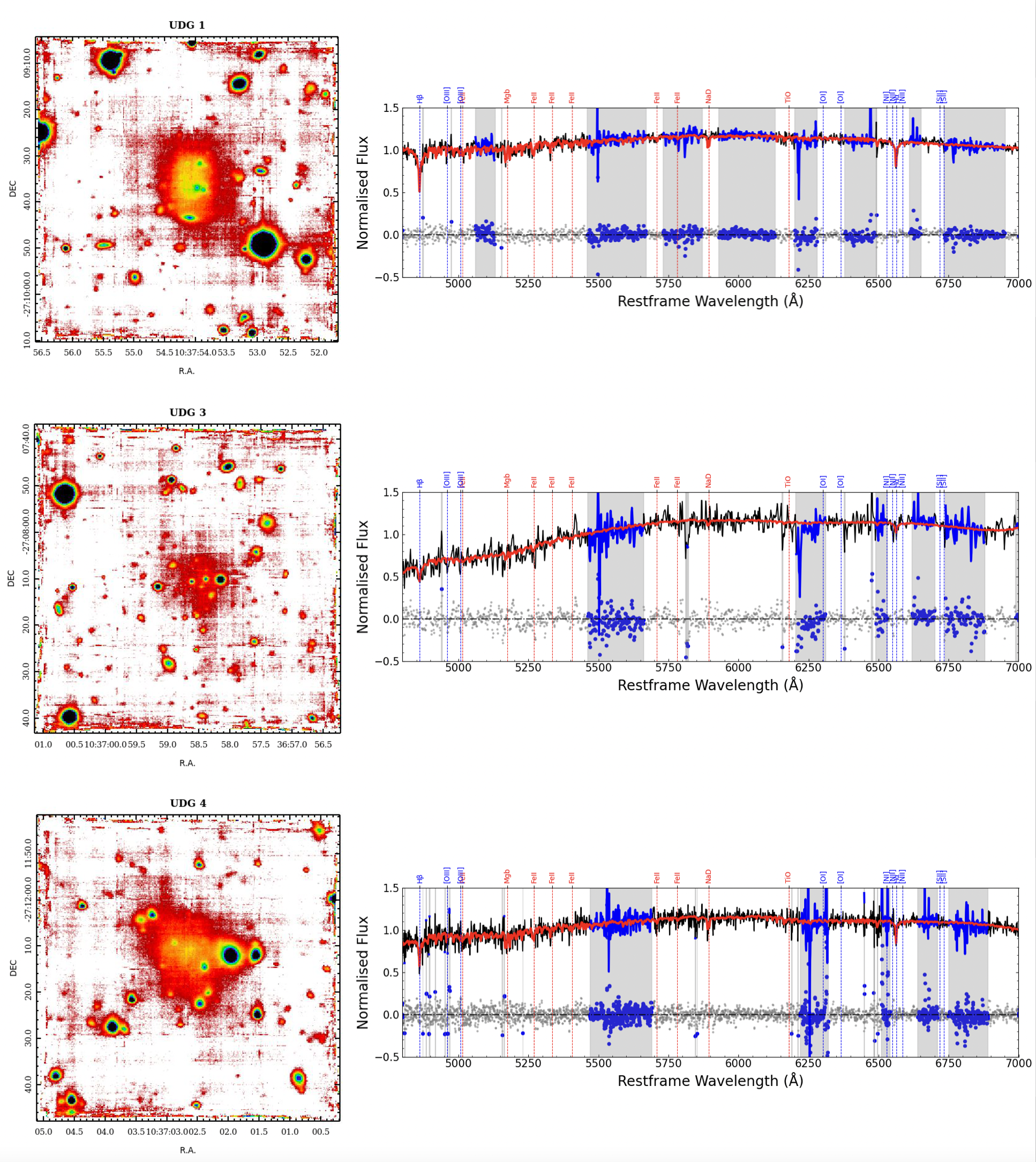
Figure 14: MUSE reconstructed images (left panels) and stacked spectra (right panels) of the observed LEWIS targets. From the top to the lower panels, UDG1, UDG3 and UDG4 are shown, respectively. The red line corresponds to the pPXF best fit using the set-up described in Sec. 4. Grey boxes mark the masked regions, excluded from the fit.

Figure 15: Same as Fig. 14, for UDG7, UDG8 and UDG9.

Figure 16: Same as Fig. 14, for UDG10, UDG12 and UDG13.

Figure 17: Same as Fig. 14, for UDG15, UDG20 and UDG21.

Figure 18: Same as Fig. 14, for UDG22 and UDG23.

Figure 19: Same as Fig. 14, for LSB4, LSB5 and LSB6.

Figure 20: Same as Fig. 14, for LSB7 and LSB8.