Bright quantum photon sources from a topological Floquet resonance

Abstract

Entanglement, a fundamental concept in quantum mechanics, plays a crucial role as a valuable resource in quantum technologies. The practical implementation of entangled photon sources encounters obstacles arising from imperfections and defects inherent in physical systems and microchips, resulting in a loss or degradation of entanglement. The topological photonic insulators, however, have emerged as promising candidates, demonstrating an exceptional capability to resist defect-induced scattering, thus enabling the development of robust entangled sources. Despite their inherent advantages, building bright and programmable topologically protected entangled sources remains challenging due to intricate device designs and weak material nonlinearity. Here we present an advancement in entanglement generation achieved through a non-magnetic and tunable resonance-based anomalous Floquet insulator, utilizing an optical spontaneous four-wave mixing process. Our experiment demonstrates a substantial enhancement in entangled photon pair generation compared to devices reliant solely on topological edge states and outperforming trivial photonic devices in spectral resilience. This work marks a step forward in the pursuit of defect-robust and bright entangled sources that can open avenues for the exploration of cascaded quantum devices and the engineering of quantum states. Our result could lead to the development of resilient quantum sources with potential applications in quantum technologies.

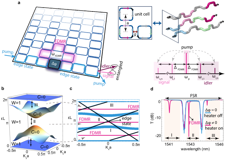
Figure 1: Schematic representation and simulation of a Floquet topological entanglement source. a, A 2D square microring lattice consisting of individual ring resonators arranged in identical unit cells. Each unit cell (inset) comprises three closely coupled microrings arranged in a square formation with the coupling strength $g$ and center-to-center distance $a$. By unrolling each microring from the points shown by black arrows, an equivalent coupled waveguide array can be obtained (inset). Four periodic coupling sequences, in the microring unit cell and in its equivalent waveguide array, are shown by light blue, light pink, light green, and dark pink arrows/segments. Gray color shows uncoupled part of microrings/waveguides. An FDMR with resonance frequency $\omega_{\mathrm{FDMR}}$ can be created by utilizing a thermo-optics effect to introduce a phase shift $\Delta\phi$ in one of the rings along the path of the edge state. The lattice’s periodicity leads to the appearance of multiple equally spaced modes, separated by the frequency of $\Delta_{\mathrm{FDMR}}$. By applying a pump to the system via the edge state and utilizing the SFWM process within the FDMR, we can produce idler-signal entangled photons at various $\Delta_{\mathrm{FDMR}}$ within the system, as illustrated in the lower inset. b, The computed band structure for the photonic anomalous Floquet topological insulator in one Floquet–Brillouin zone with wavenumbers $K_{x}$ and $K_{y}$, comprising one unit cell periodic in both $x$ and $y$ directions. The transmission bands of Floquet states, with Chern number $C=0$, are separated by three topological bandgaps, labeled by (I, II, II), with Winding number $W=1$. c, Projected band diagrams of a semi-infinite lattice limited in the $y$-direction (consisting of 10 unit cells) and extending infinitely in the $x$-direction. The red bands represent the flat bands of Floquet bulk, obtained using a semi-infinite $5\times 5$ supercell, which are distinct from the transmission band manifolds due to a phase detune. d, Simulated transmission spectra of an ideal topological photonic insulator lattice of identical microring resonators with power coupling of $98\%$, considering intrinsic loss, in the presence (pink line) and absence (blue line) of the phase shift $\Delta\phi$.

The unique properties of entanglement and topology hold tremendous potential for advancing quantum technology. Entanglement has emerged as a crucial resource in quantum information [1, 2]. Its applications span diverse disciplines, including quantum sensing [3, 4], computing [5, 6], and communication [7, 8]. Significant progress has been made in the optical domain, especially concerning the generation of entangled states through integrated devices [9, 10], opening up avenues for practical real-world applications [11, 12, 13, 14]. However, preserving and effectively harnessing entanglement face challenges due to inevitable fabrication imperfections and defects in the microchips [15, 16]. These disorders can lead to loss, scattering, and spectral randomness, ultimately affecting the stability and purity of the entanglement [17, 18].

Similarly, topological photonic insulators (TPIs) have attracted considerable attention due to their ability to guide light through topologically-protected edge states [19, 20, 21]. These states have found applications in various domains such as lasing [22, 23, 24], soliton generation [25, 26] and frequency comb [27]. The most intriguing aspect of TPIs is their resilience to scattering caused by defects, making them highly desirable for robust device development, capable of withstanding fabrication imperfections encountered during photon transport [28, 29, 30]. Therefore, utilizing TPI systems for generating nonclassical emissions offers unprecedented possibilities for advancing quantum technology.

Recently, TPIs have been employed for generating robust entangled photons emission using coupled waveguides [31] and microring resonators [32, 33], as well as through Floquet-based TPIs [34]. Nevertheless, the practical implementation of nonclassical sources based on edge states has faced challenges due to the weak nonlinear properties of the materials. Ensuring sufficient pair generation requires either long lattice boundaries, leading to increased material loss, or utilizing high pump powers that introduce noise and reduce the purity of the entanglement. These limitations have constrained the potential applications of TPIs in quantum technologies, especially in scenarios demanding bright entangled emissions, such as long-distance quantum communications. Despite demonstrating resonance enhancement of photon pair generation through spontaneous four-wave mixing (SFWM) in conventional resonators [35, 36, 37, 38, 39, 40], the experimental realization of a bright Floquet TPI entanglement source has remained elusive and unexplored until now.

Here for the first time, we explore entanglement generation in a novel resonance effect called Floquet Defect Mode Resonance (FDMR) in the bulk of a Floquet TPI [41]. We present compelling experimental evidence that demonstrates a substantial enhancement in entangled photon pair generation by harnessing this compact topological cavityless resonance effect. By exciting the wavelength-tunable FDMR and utilizing SFWM in a silicon microring lattice coupled to a topologically-protected edge state, we successfully create a bright quantum photon source. This source demonstrates a second-order cross-correlation of photon pairs approximately 3300 times higher compared to using edge mode without resonance. These results demonstrate the potential of FDMR in significantly improving the efficiency of entangled photon pair generation in TPI-based systems, thereby removing the necessity for high power or extended chip boundaries. Our topological quantum device combines the advantages of integrated topological photonics, tunable localized optical modes, and robustness to disorder, representing a novel approach to generating entangled photon pairs. Such an approach holds great promise for various applications, including the advancement of ultrabright photon-pair generation for quantum information processing and facilitating the development of TPI high-dimensional entangled quantum states [42] as well as quantum logic [43].

Anomalous Floquet resonance mode

Fig. 1a presents the schematic of our Floquet topological photonic insulator, created using two-dimensional (2D) directly-coupled microring resonators [44]. Each unit cell, see the inset of Fig. 1 a, comprises three strongly coupled identical microrings arranged in a square shape with the coupling coefficient $g$. As light propagates around each microring, it evanescently couples to the neighboring rings in a periodic sequence, see Fig. 1(a), with the period equal to the microring circumference $L$. The system thus emulates a periodically driven system with the evolution along the direction of light propagation $z$ rather than time [45]. By varying the coupling between microrings, the topological phase of the lattice can be tuned, leading to the appearance of Chern or anomalous Floquet topological insulators in the weak or strong coupling regimes, respectively as shown in Refs [46, 45, 34]. Our 2D microring lattice follows a similar framework as the Floquet systems and satisfies the following eigenvalue equation for the wavefunction $|\psi_{n}(\textbf{k})\rangle$

$$U_{F}(\textbf{k})|\psi_{n}(\textbf{k})\rangle=e^{i\epsilon_{n}(\textbf{k})L}|\psi_{n}(\textbf{k})\rangle,$$ (1)

where $\epsilon_{n}(\textbf{k})$ is the quasi-energy band of the lattice with the periodicity of $2\pi/L$. The Floquet operator $U_{F}(\textbf{k})=\mathcal{T}e^{i\int_{0}^{L}H(\textbf{k},z^{\prime})dz^{\prime}}$, where $\mathcal{T}$ represents the time-order operator, depends on the Floquet-Bloch Hamiltonian $H(\textbf{k},z)=H_{\mathrm{FB}}(\textbf{k},z)$ that exhibits periodicity along the $z$ direction $H(\textbf{k},z)=H(\textbf{k},z+L)$, with a period of $L$. This characteristic mimics the behavior of a periodically driven Hamiltonian, where the variable $z$ plays the role of time $z\rightarrow{t}$. We can obtain an expression for $H(\textbf{k},z)$ by transforming the microring lattice into an equivalent coupled waveguide array, see the inset of Fig. 1a. In the strong coupling regime, our 2D lattice exhibits three bandgaps with non-zero Winding numbers. All bands possess trivial Chern numbers $C=0$, making it an anomalous Floquet insulator, as shown in the band structure of one Floquet-Brillouin zone of the unit cell in Fig. 1b. To verify the presence of topological edge states, we impose boundaries along the $y$-axis while assuming the lattice extends infinitely along the $x$-axis. From the projected quasi-energy band diagram, we observe the existence of two pseudospin topological edge states in each bandgap, as shown in Fig. 1c.

By exploiting the natural hopping sequence of our 2D lattice and leveraging the edge state’s resilience against local defects, we can achieve the confinement of light within a closed loop, creating a cavityless local resonator. This confinement is attained by introducing a small perturbation in the driving sequence, in the form of a phase shift ($\Delta\phi$), in one of the ring resonators along the edge state’s trajectory, leading to the formation of a flat-band Floquet mode within the 2D lattice. As a result, the light becomes effectively trapped within the loop, giving rise to a locally confined mode referred to as FDMR. This perturbation subsequently modifies the total Hamiltonian of the system $H=H_{\mathrm{FB}}+H_{\mathrm{FDMR}}$ where $H_{\mathrm{FDMR}}=\hbar\omega_{\mathrm{FDMR}}a^{\dagger}a$ describes the FMDR with a resonance frequency $\omega_{\mathrm{FDMR}}$ and annihilation operator $a$. The associated quasienergy of this mode experiences a shift directly proportional to the magnitude of the induced phase, as depicted in Fig. 1c (see Supplementary Materials). This FDMR mode can achieve a large Q-factor, approaching $10^{5}$, compared to other 2D topological resonators [47, 48], mainly because it lacks physical boundaries that would otherwise confine light within the defect resonator. The resonance pattern in FDMR follows the trajectory of the topologically nontrivial Floquet bulk mode with a total circumference of $3L$. Fig. 1d illustrates the simulation of the transmission spectrum of our design in the presence and absence of a phase shift, demonstrating the appearance of the FDMR. Note that, this mode is coupled to the edge state existing within the same bandgap, implying that we can control or access the FDMR via the edge state.

To generate correlated photon pairs through the SFWM process within the bandgap of the topological 2D lattice, we utilize the third-order nonlinearity $\chi^{3}$ in silicon. The Hamiltonian that describes this process is given by

$$H_{\mathrm{non}}=\hbar g_{\text{nl}}\big{(}a_{p}a_{p}a_{s}^{\dagger}a_{i}^{\dagger}+h.c\big{)},$$ (2)

where $g_{\text{nl}}$ is the strength of the SFWM while $a_{p}$ and $a_{s(i)}$ refer to the annihilation operators of the pump and signal (idler) modes, respectively. The Hamiltonian (2) represents a four-photon mixing process in which two photons from the pump are annihilated, resulting in the creation of photons in the idler and signal modes, which were initially in a vacuum state. With the presence of the FDMR, the generation of the photon pairs is significantly enhanced, surpassing the pair generation rate achieved solely with the edge state

$$N_{\mathrm{FDMR}}\propto N_{\mathrm{edge}}\times Q^{3},$$ (3)

where $N_{\mathrm{FDMR}}$ and $N_{\mathrm{edge}}$ are the pair generation rates of the FDMR and edge state, respectively and $Q$ is the quality factor of the FDMR, see the Supplementary Materials.

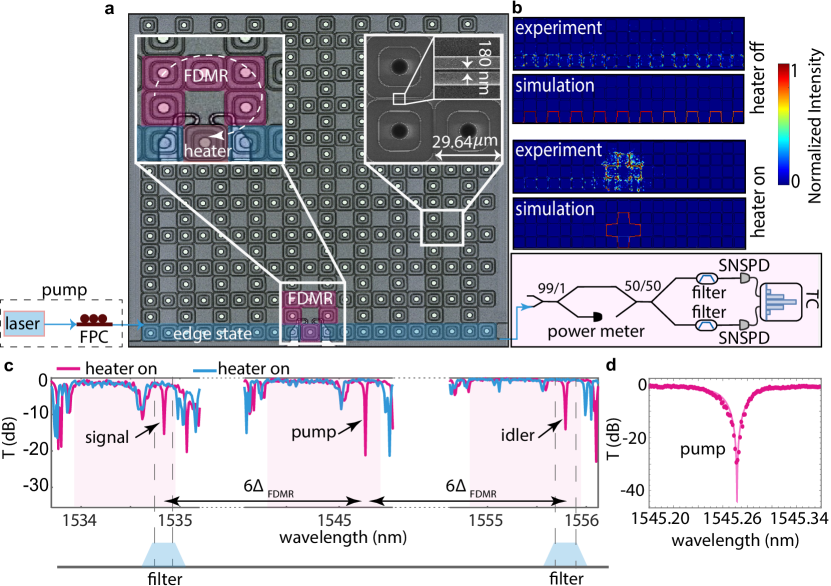
Figure 2: Experimental realization. a, A microscopic image of the anomalous Floquet insulator lattice, featuring a $10\times 10$ unit cells arrangement across a $595.32\times 595.32$ $\mu$m chip. The insets provide detailed scanning electron microscopy (SEM) views of a unit cell and the structure of the heater functioning as a thermo-optics phase shifter. Each microring in our design has a square shape, with side lengths of 29.64 $\mu$m, and rounded corners with a radius of 5 $\mu$m to minimize scattering losses. Additionally, the figure includes a diagram of the experimental setup, which involves a pump laser passing through a fiber polarization controller (FPC) and being injected into the sample via a lensed fiber. The transmitted light is measured using a photon detector and a power meter, two narrow bandpass filters, two Superconducting Nanowire Single-Photon Detectors (SNSPDs), and a Time Controller (TC). b, Near Infrared images of the edge state and FDMR in real-time and comparison with numerical simulations. c, The normalized transmission (T) of the lattice as a function of the pump wavelength. The solid line represents the fitted theoretical model, as detailed in the Supplementary Materials. d Zoomed-in transmission of the FDMR with respect to the wavelength of the pump.

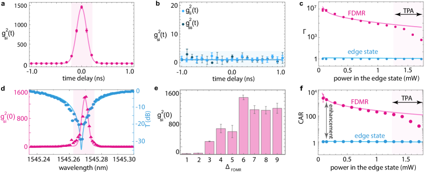
Figure 3: Enhancement of the photon pairs generation. a and b, show the measured second-order cross-correlation $g_{si}^{(2)}(t)$ and the second-order autocorrelation function $g_{ss/ii}^{(2)}(t)$, respectively, for the power in edge state of 0.29 mW. c, Obtained nonclassical parameter, $\Gamma$, for both FDMR and edge state at different pump powers. Increasing the pump power pushes the system to a nonlinear regime such as the two-photon absorption (TPA). d, Illustrates the transmission and $g_{si}^{(2)}(0)$ versus pump wavelengths around the resonance frequency of the FDMR for the pump power of 0.29 mW. e, Shows the measured $g_{si}^{(2)}(0)$ at different $\Delta_{\mathrm{FDMR}}$ at the same powert. f, Display the obtained CAR for FDMR and edge state versus pump power in the edge state. For all panels, the error bars are derived from three independent measurements. For some points, the size of the dots is larger than the error bars. Fitted solid lines in panels a and b utilize the Poissonian distribution while fitting for panels c, d, and f is based on the comprehensive theory outlined in the Supplementary Materials.

Results

We experimentally demonstrate the generation and enhancement of entangled photons within our 2D Floquet lattice. The lattice is structured with a $10\times 10$ unit cell arrangement and fabricated on a Silicon-on-Insulator (SOI) substrate, incorporating a total of 300 individual ring resonators, see Fig. 2a. Each microring in our design is square-shaped and is designed to achieve efficient power coupling, enabling around $g^{2}=98\%$ of the power transfer from one microring to the nearest microring. This design is specifically chosen to achieve the desired anomalous Floquet insulator behavior around the wavelength of 1545 nm.

Fig. 2b presents the real-time field distribution for the edge state and FDMR, as measured via a Near-Infrared camera. These experimental results demonstrate excellent agreement with the numerical simulations obtained by solving the Schrödinger equation. In particular, the edge state exhibits distinct nontrivial light propagation along the boundaries of the lattice. By applying a phase shift in a microring located on the bottom edge of the sample, we observe the emergence of the FDMR mode, characterized by a strongly localized field distribution in a loop pattern.

The chip’s transmission spectrum is measured by injecting a laser into the lattice at the bottom left edge and detecting the output light at the bottom right edge using a powermeter, as displayed in Fig. 2a. During the measurement, the laser’s wavelength is swept from 1530 nm to 1557 nm, equivalent to 13 $\Delta_{\mathrm{FDMR}}$. Note that we define $\Delta_{\mathrm{FDMR}}$ as the frequency spacing of the FDMR which is approximately one-third of the FSR of our TPI, measuring 1.72 nm. The normalized transmission spectrum, shown in blue in Fig. 2c, allows us to identify topologically nontrivial bandgaps, characterized by regions of high and flat transmission as labeled by (I, II, and III). Upon activation of the heater (phase shift), a Floquet bulk mode is lifted into the bandgap, resulting in a flattened energy band and a resonant mode spatially localized in a loop pattern, as demonstrated at the bottom of Fig. 2a (see the inset). The transmission spectrum in the output waveguide, with a phase detune of $\Delta\phi=2.37\pi$, is represented by the pink trace in Fig. 2c. The presence of distinct and adjustable resonance dips within each bandgap of each FSR of the device indicates the excitation of a resonance mode that is coupled to the edge state. In Fig. 2d, a close-up view of the transmission and the theoretical fit for a selected mode is shown. This mode will be utilized for resonance-enhanced entanglement generation.

To generate entangled photon pairs using FDMR, we employ a continuous-wave pump beam with a frequency that corresponds to one of the FDMRs with a $Q=4.843\times 10^{4}$, as indicated by an arrow in Fig. 2c. Maintaining energy conservation via the SFWM process requires the generation of photon pairs for idler and signal modes at different $\Delta_{\mathrm{FDMR}}$ symmetrically distributed around the pump frequency. To measure photon pairs that fulfill this condition and suppress the emission from FDMR modes in different $\Delta_{\mathrm{FDMR}}$, we utilize two narrowband tunable filters. These filters have center wavelengths placed at $6\Delta_{\mathrm{FDMR}}$, both below and above the pump wavelength, see Fig. 2c. This setup enables efficient selection of the desired entangled photon pairs while minimizing interference from unwanted FDMR modes at different $\Delta_{\mathrm{FDMR}}$. We verify the non-classical nature of the photon pairs generated from FDMR by measuring the second-order cross-correlation function defined by $g_{si}^{(2)}(t)=\frac{\langle\hat{n}_{s}\hat{n}_{i}\rangle}{\langle\hat{n}_{s}\rangle.\langle\hat{n}_{i}\rangle}$, where $\hat{n}_{s/i}$ is the photon number of the signal/idler modes. This function determines the normalized probability of detecting signal and idler photons at a specific time separation $t$ and can be measured using coincidence rates of the signal-idler pairs and individual photon counts, see Methods.

Fig. 3a shows the measured second-order cross-correlation function, with a maximum value of $g_{si}^{(2)}(t)\approx 1450\pm 50$ observed at $t=0$ and at a fixed pump power of $0.29$ mW, compelling evidence of time-correlated photon pairs at the FDMR. At the same power, we compare these results with the second-order autocorrelation functions, $g_{ii}^{(2)}(t)\approx 1$ and $g_{ss}^{(2)}(t)\approx 1$, for the idler and signal modes, shown in Fig. 3b. This comparative analysis allows us to examine a formal proof of a non-classical light source i.e. the violation of the Cauchy-Schwarz inequality, $\big{[}g_{si}^{(2)}(0)\big{]}^{2}\leq\big{[}g_{ss}^{(2)}(0)\cdot g_{ii}^{(2)}(0)\big{]}$. Alternatively, we define and measure the nonclassicality parameter

$$\Gamma:=\frac{\big{[}g_{si}^{(2)}(0)\big{]}^{2}}{\big{[}g_{ss}^{(2)}(0)\cdot g_{ii}^{(2)}(0)\big{]}},$$ (4)

for which $\Gamma>1$ indicates a nonclassical source. Fig. 3c illustrates measurements of the parameter $\Gamma$ as a function of the pump power and includes a comparison with the photons generated from the edge state when the FDMR mode is absent. The plot shows the violation of the Cauchy-Schwarz inequality ($\Gamma>1$), indicating a profound enhancement of nonclassical properties in the emitted photons due to the presence of the FDMR and its coupling to the edge state, which effectively increases the cross-correlation. The experimental result is in good agreement with the theoretical model we developed in the Supplemental Materials except at high powers region where the nonlinear effects, such as two-photon absorption (TPA) and pump noise change the single and coincidence count rates. We note that the small size of our chip limits the edge state’s ability to generate significant photon pairs while propagating at the shorter arm of the sample. Hence, unlike Ref. [32] the measured emission from the edge state is primarily composed of pump leakage and lacks considerable nonclassical properties i.e. $\Delta\approx 1$.

Table 1: Comparing the result of entangled photon pairs generation around the $1.55\,\mu$m wavelength, achieved through optically-driven SFWM. Micro-ring resonator ($\mu$-ring), coupled resonator optical waveguide (CROW), topologically protected (TP), pair generation rate (PGR), coincidence-to-accidental rate (CAR), cavityless or not physical boundary.

Integrated photonic sources	On-chip power ($\mu$W)	CAR	PGR	Dimension	TP	Cavityless	Coupling to edge state
$\mu$-ring [39]	7.4	12100	16 kHz	1D	No	No	No
Coupled $\mu$-rings [40]	12	1100	200 Hz	1D	No	No	No
CROW [35]	200	80	1.64kHz	1D	No	No	No
Topological based/edge state [32]	1400	42	-	2D	Yes	-	-
This work	86	2331	30kHz	2D	Yes	Yes	Yes

To investigate the resonance-enhancement of the FDMR, at the pump power of 0.29 mW, the wavelength of the pump was swept across one resonance, allowing for $g_{si}^{(2)}(0)$ to be compared to the transmission of the FDMR, as shown in Fig. 3d. The peak of cross-correlation, pink trace, coincides with the deepest point of the resonance, blue trace, demonstrating successful resonance enhancement of the generation of entangled photon pairs, with 2nd-order cross-correlation up to $\approx$1450. We also measured the $g_{si}^{(2)}(0)$ at different $\Delta_{\mathrm{FDMR}}$ in Fig. 3e.

Another important parameter for evaluating the nonclassical properties of the generated photon pairs is the Coincidence to Accidental Rate (CAR). It serves as a reliable indicator of the signal-to-noise ratio of the entangled photons and is obtained by integrating $g_{si}^{(2)}(t)$ over the peak at $t=0$. The CAR is measured as $\mathrm{CAR}\propto\frac{N_{c}}{N_{s}N_{i}}$, where $N_{c}$ represents the coincident count rate, and $N_{s/i}$ denotes the single count rates of the signal/idler. Note that, all three count rates $N_{j}$ ($j=c,s,i$) scale quadratically with the pump power (see Methods), resulting in the observed inverse dependence of CAR with the square of power in agreement with our theoretical model, see Fig. 3f. This figure also provides a comparison of the CAR between the FDMR and the edge state (heater off) under various pump powers. Our source achieves an exceptional CAR value of $2300$, significantly surpassing the $\mathrm{CAR}\approx 1.01$ obtained with edge states in the absence of the FDMR. Moreover, this performance exceeds what is typically achieved with other similar sources utilizing edge states in larger chips and topologically trivial single and cascaded ring resonators. The result highlights the outstanding performance of the FDMR in enhancing the nonclassical characteristics of the generated photons. In Table 1, we compare our Floquet entangled source and the current state-of-the-art photon-pair sources in silicon. Unlike basic microring resonators [35, 39, 40], FDMR has the capacity to be turned on and off in situ while also having the capability to couple with edge states. Multiple FDMRs can be activated and coupled on a single chip. These characteristics distinguish our system from the traditional approach of entanglement generation using microring resonators.

Discussion

In summary, we have demonstrated the resonance-enhanced generation of entangled photon pairs within anomalous Floquet TPI, operating at room temperature. This achievement is made possible by employing an FDMR coupled to a topological edge mode. To verify the nonclassicality of the generated entangled photons, we conducted measurements of the second-order cross-correlation, tested the nonclassical characteristic of the emission, and provided a comparison with the comprehensive theoretical model that we have developed.

We conclude our discussion by exploring the topological protected properties of our system. Unlike previous approaches that depend on propagating fields in the edge state to generate photon pairs, our approach distinctively employs a confined mode embedded within the bandgap region co-existing with the edge state. Therefore, the FDMR operates as a frequency-tunable source that generates entangled pairs, while the edge state acts as a topologically protected waveguide that delivers the generated photons to the output ports. Consequently, our system acquires the same topologically protected features as those inherently present within the edge state. This unique capability sets the current system apart from other sources of entanglement based on edge state [32, 33, 34], as well as from the topologically trivial photonic devices [35, 36, 37, 38, 39, 40]. We note that defects and disorders at the physical boundaries, where the FDMR forms, have the potential to interfere with the loop, reduce the mode’s quality factor or shift the mode. However, the frequency tunability of the FDMR can partially mitigate these effects. In the Methods, we expand further this discussion and explore various defects along with their impact on the FDMR.

An essential aspect of our sample is its capability to generate entanglement within a relatively small chip due to the compact size of the FDMR. This feature becomes especially crucial when the material loss of the sample affects the nonclassical property of the photon pairs. The compact nature of the FDMR allows for efficient entanglement generation and on-chip distribution, making it well-suited for scenarios where larger devices might encounter challenges related to propagation loss. The exceptional attributes of the FDMR, including its high quality factor, compact size, tunability (on and off), and coupling with the edge state play a critical role in facilitating the generation of bright entangled photon pairs. It opens up possibilities for exploring novel techniques of on-chip entanglement distribution, field-matter interaction, and advancing integrated quantum electrodynamics. In particular, the FDMR can efficiently interact with localized atoms/ions in the substrate, facilitating their integration into a network of cascaded atom-cavity chains connected with edge states. This platform holds promise for the development of on-chip and topologically-protected quantum computing and processing.
Acknowledgments We thank Mohammad Hafezi for helpful comments and discussions and Tyler Zegray for preparing the figures. S.B. acknowledges funding by the Natural Sciences and Engineering Research Council of Canada (NSERC) through its Discovery Grant, funding and advisory support provided by Alberta Innovates (AI) through the Accelerating Innovations into CarE (AICE) – Concepts Program, support from Alberta Innovates and NSERC through Advance Grant project, and Alliance Quantum Consortium. V.V. and T.J. acknowledge funding from NSERC and AI. This project is funded [in part] by the Government of Canada. Ce projet est financé [en partie] par le gouvernement du Canada.
Contributions S.B. and V.V. conceived the ideas. S.B, S.A, T.Z. T.H. and V.V. developed and built the experimental setup. S.B., S.A, M.R, and M.T. analyzed the data. S.B., S.A. T.Z, and M.R. developed the theoretical model and performed the measurements. V.V., T.Z., and S.A. simulated and fabricated the sample. S.A. designed the chip. S.A. and M.K. developed the measurement codes. All the authors contributed in preparing the manuscript.
Disclosures The authors declare no conflicts of interest.
Data Availability Statement Data underlying the results presented in this paper are available upon proper request.

Methods

Device design and Fabrication

We conducted device simulations using Lumerical software with the Mode Solution and Finite-Difference Time-Domain solver. Our simulations involved introducing a TE-polarized mode into waveguide couplers, where the coupling lengths matched the side length of the squared ring. From the simulation results, we calculated the coupling angle $\theta$ and power coupling coefficient $g^{2}=\text{sin}(\theta)^{2}$. Subsequently, we designed the sample and fabricated the device on an SOI chip. The silicon waveguides within our TPI have dimensions of 450 nm in width and 220 nm in height, while the cladding consists of $2\mu$m of top SiO₂ and $2.2\mu$m of bottom SiO₂. Our design includes square-shaped microrings with side lengths of 29.64 $\mu$m, and we integrated rounded corners with a radius of 5 $\mu$m to minimize scattering losses. To achieve efficient power coupling, we precisely set the gaps between the microrings at 180 nm, enabling approximately $98\%$ of power transfer from one microring to the next-nearest microring. This particular design was chosen to attain the desired anomalous Floquet insulator behavior at a wavelength of 1545 nm.

Activation of the FDMR

We initiate the excitation of an FDMR and achieve precise tuning of its resonant frequency by manipulating the phase of one of the ring resonators situated on the lower boundary of the lattice. To facilitate this tuning process, we fabricate a titanium-tungsten (TiW) heater, which covers the rectangular perimeter, and apply current to the heater. As we perform this manipulation, we observe that the resonant wavelength shift $\delta\lambda$ of the FDMR exhibits an approximately linear relationship with the applied heater power $p_{\text{heat}}$, see Supplementary Methods.

Measurement setup

Fig. 2a illustrates our experimental setup designed to test the correlation between the generated photon pairs and evaluate their quantum properties. The setup involves the following components: TE-polarized pump photons generated by an FPC and a tunable continuous-wave laser (Santec TSL-550) at telecom wavelengths. The laser output power ranges from 0.086 mW to 1.73 mW, delivered via a lensed-tip fiber that is butt-coupled to the chip’s facet. The pump and generated wavelengths are collected at the output fiber, with $1\%$ of the light sent to a photon detector and a power meter to measure the device’s transmission spectrum. The remaining light is split into two separate paths using a 50/50 coupler. The signal and idler photons then pass through bandpass filters (Optoplex C-Band 50GHz) to suppress the input pump light by 40dB, as well as other generated photons at different frequencies. Finally, two SNSPDs ”ID Quantique - ID281” detect isolated photons, providing electrical signals to a Time Controller (ID900) with a timing resolution of 100ps.

In our experiments, we initially inject 1mW of pump power from the laser into the lattice at the bottom left edge. We measure the output light from the bottom right edge while sweeping the laser wavelength from 1530nm to 1557nm (5 FSR of the TPI). The total loss from the laser to the power meter is measured as -10.5 dB, accounting for input and output coupling losses (from fiber to chip and vice versa), FPC, and loss in the chip. The losses in the FPC and the chip are measured as 0.24 dB and 2.6 dB/cm, respectively. As a result, for 1mW laser power, the power in the waveguide is estimated as 0.29 mW. The transmission spectrum before and after applying phase detuning is shown in Fig. 2c, respectively by blue and pink traces.

Single and coincidence counts measurement

Taking into account the losses in both the signal and idler channels, the measured coincidence rate can be expressed as $N_{\text{tot},c}=\eta_{i}\eta_{s}N_{c}$, where $\eta_{s/i}$ represents the transmission efficiency from the chip’s output to the SNSPDs, and $N_{c}$ denotes the inferred coincidence rate excluding measurement losses and efficiencies (see Supplementary Materials). In addition to system losses, for the measured signal and idler pair rate, we must consider the noises and residues related to the sidebands of the pump and pump leakage, which exhibit a linear relationship with pump power ($N_{s/i,p}\propto P$). Furthermore, we account for the extra counts associated with the dark counts $D_{s/i}\approx 50$ Hz of the SNSPDs. Consequently, the measured single/idler counts rate can be defined as follows

$$N_{\text{tot},s/i}=\eta_{s/i}N_{s/i}+N_{s/i,p}+D_{s/i}$$ (5)

where $N_{s/i}$ signifies the inferred signal/idler single count rates. In Fig. 4a, we plot the inferred $N_{c}$ as a function of the pump power in the edge state. As anticipated, the coincidence rate exhibits a rise with the increasing pump power.

Second-order correlation function and coincidence-to-accidental rate

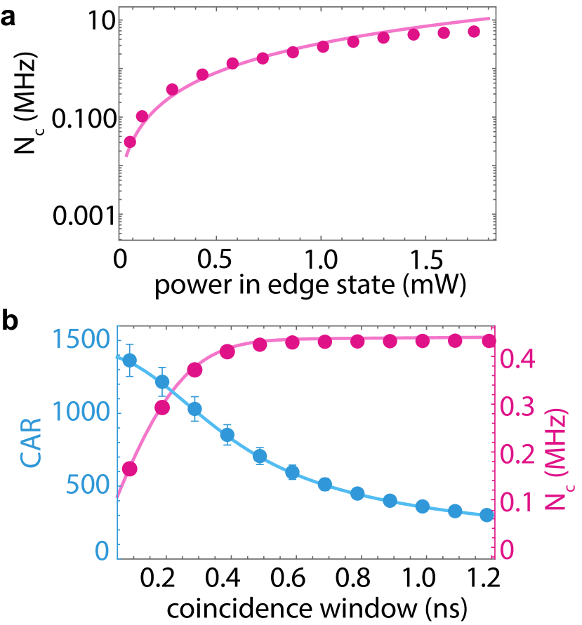
Figure 4: a Coincidence rate $N_{c}$ versus the pump power in the edge state. b Dependency of CAR and coincidence rate $N_{c}$ to the measurement coincidence window.

To characterize the correlation of the generated photon pairs, we use the second-order cross-correlation function $g_{si}^{(2)}(t)$ by measuring single and coincidence counting methods employing the SNSPDs and the Time Controller (TC). This function allows us to determine the normalized probability of detecting signal and idler photons with a time separation of $t$ [49]:

$$g_{si}^{(2)}(t)=\frac{N_{\text{tot},c}}{N_{\text{tot},s}N_{\text{tot},i}}\times\frac{1}{T_{\mathrm{coin}}}$$ (6)

where $T_{\mathrm{coin}}$ is the duration of arrival time called the coincidence window. We analyzed the second-order cross-correlation function $g_{si}^{(2)}(t)$, within the smallest measurable coincidence window, 100 ps, of our Time Controller.

The determination of the coincidence-to-accidental rate (CAR) involved using the coincidence histogram. We achieved this by calculating the ratio of the total coincidence counts, within a coincidence window centered around the peak values, to the accidental counts recorded during the same coincidence window [50]

$$\text{CAR}=\frac{\int_{-t/2}^{t/2}g^{2}_{si}(t)dt}{\int_{\infty-t/2}^{\infty+t/2}g^{2}_{si}(t)dt}.$$ (7)

To obtain the proper coincident window, we first fitted the coincidence counts using a Gaussian function to calculate the variance, $\delta=99.7$ ps, and the full-width half maximum (FWHM) of the coincidence counts as $\text{FWHM}=2\sqrt{2\text{ln}2}\delta=234.8$ ps. Fig. 4 b shows the integration of coincidence count rates, $N_{c}$, over various coincidence windows and their corresponding CARs. As shown in this figure, there is a triad-off between the coincidence rate and CAR at different time windows. Since the coincidence rate gets saturated at coincidence windows greater than 0.5 ns, leading to dropping CAR, we consider the coincidence window$=3\delta\approx 1.2\text{FWHM}=0.3$ ns to calculate CAR at different pump power shown in Fig. 3f.

Resiliency against defect

We emphasize that the nature of FDMR mode comes from the topologically nontrivial behavior of the lattice, in that, the existence of circulating loops in the bulk of the lattice [41, 26] is required to mimic the quantum hall effect that pushes the light to propagate only at the edge of the lattice unidirectionally. In fact, the topology of the lattice makes FDMR loops to be robust to fabrication imperfections as long as the defect doesn’t completely alter the hopping sequence, for instance, by removing one ring in the loop where the FDMR is excited.

To illustrate the resilience of FDMRs, we conducted simulations of the lattice’s transmission spectrum, considering deviations of $10\%$ and $20\%$ in coupling coefficients between microrings and variations in the roundtrip phase of each microring. Our simulations encompassed 50 lattices, incorporating random variations centered around the FDMR loop. The most significant impacts on the transmission spectrum are presented in Fig. 5, shown by the dark green and light blue lines for coupling coefficient and roundtrip phase variations, respectively. This illustration confirms that specific types of defects, whether within the FDMR loop or adjacent microrings, manifest as loss channels. While these defects may alter the quality factor of the FDMR resonance or cause a resonance shift, they are unable to destroy the FDMR loop.

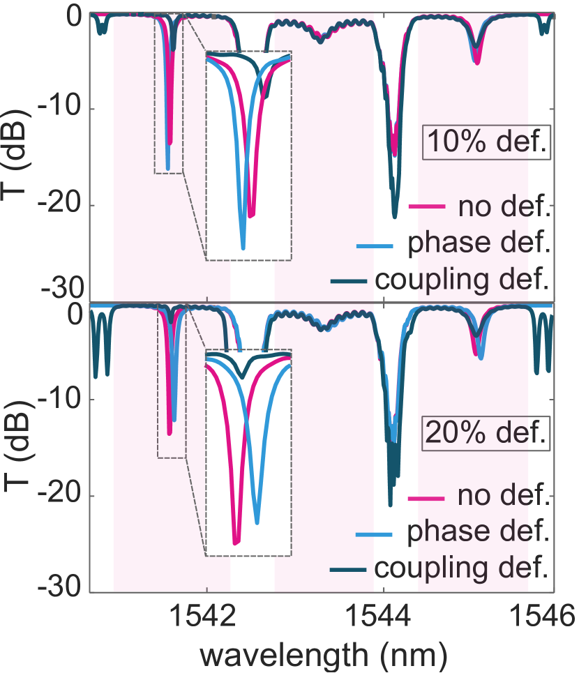
Figure 5: Robustness of FDMR vs fabrication imperfections. a and b, Simulation of respectively $10\%$ and $20\%$ variations in coupling coefficient between microrings and roundtrip phase of the microrings located around the FDMR resonance. Pink lines represent the lattice without defects. Light blue and dark green lines show the maximum changes in FDMR due to coupling defects and roundtrip phase defects, respectively. The maximum change,in terms of both frequency shift and resonance linewidth, are chosen from 50 simulations with random defects in the coupling coefficient representing the variations in the gaps between microrings and roundtrip phase defects which are due to variations in the size of the microrings. As illustrated in this figure the defects in the roundtrip phases cause shifts in resonance and defects in $g$ lead to changes in the Q-factor of the FDMR.

As discussed above, various forms of defects and disorders can appear within our devices. This section aims to elaborate further on distinct scenarios that could potentially impact the efficiency of our system.

1. Defect affecting the edge state: A possible scenario involves the emergence of defects/disorders along the trajectory of the edge state, far away from the region where the FDMR forms. In such an instance, the system demonstrates resilience in the face of defects. The spectral characteristics of the system remain largely unaffected by the presence of such a defect [34]. It is worth noting that this resilience pertains specifically to certain types of defects, as the edge state remains robust against select anomalies. For instance, consider the case of sidewall roughness in the waveguide, which has the potential to induce back-reflection within the device.

2. Impact on neighboring unit cells of the FDMR: In this scenario, the presence of defects surrounds the FDMR mode, yet they do not directly intersect the FDMR loop itself. Instead, the adjacent unit cells function as loss channels, taking energy and photons away from the FDMR mode. Consequently, the introduction of these neighboring defects results in increased intrinsic losses for the mode. Such imperfections in fabrication can manifest in various ways, such as by fluctuations in the spacing between rings composing the FDMR and those situated within neighboring unit cells. These variations exert a direct influence on the overall quality factor of the mode. It’s important to highlight that the mode remains resilient against these defects, provided they do not exceed a certain magnitude (e.g., the absence of a ring within the FDMR). This assertion finds support in our simulation results, depicted in Fig. 5.

3. Defects impacting the FDMR loop: The third category encompasses defects that directly affecting on the rings forming the FDMR. This type of defect yields significant importance. It shares similarities with the second type, potentially inducing frequency shifts due to disordered configurations and resulting in phase alterations. Moreover, these defects possess the capacity to influence the quality factor of the FDMR mode by introducing surface roughness or causing partial light scattering toward adjacent rings. Another consequence involves the potential disruption of extrinsic coupling with the edge state. Such disruptions can yield variations in extrinsic quality factors, either increasing or reducing them. These defects, although impactful, do not possess the capability to destroy the entire mode, as long as the defect’s size remains proportionally smaller than that of a single ring within the loop. Fig. 5 shows simulations depicting these specific defects. Furthermore, we note that the mode’s inherent frequency tunability plays a crucial role in mitigating the effects of defects, particularly those resulting in phase shifts within the loop.

.1 Topological Photonic Insulators

The Floquet-Bloch Hamiltonian of our 2D microring lattice can be derived using a similar approach as for the general 2D microring lattice in [45], except here each unit cell contains three microrings instead of four. We first transform the microring lattice into an equivalent 2D coupled waveguide array by ”cutting” each microring in a unit cell and unrolling it into a straight waveguide with length $L$ equal to the circumference of the microring. Thus, each roundtrip of light circulation in a microring is equivalent to light propagation along the coupled waveguide array of length $L$, which can be divided into a sequence of 4 coupling steps of equal length $L/4$. Denoting the fields in microrings A, B, and C in unit cell $(m,n)$ in the lattice as $\psi_{m,n}^{A},\psi_{m,n}^{B}$ and $\psi_{m,n}^{C}$, respectively, we can write the equations for the evolution of light in the waveguide array along the direction of propagation ($z$-axis) over each period in terms of the coupled mode equations:

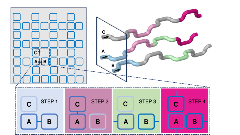
Figure 6: Mapping the coupling sequence of a 2D microring unit cell in the direction of propagation ($z$). The coupled waveguide array is obtained by unrolling the microrings in a unit cell from the points shown by black arrows.

$$-i\frac{\partial{\psi_{m,n}^{A}}}{\partial{z}}=\beta\psi_{m,n}^{A}+k_{a}(1)\psi_{m,n}^{B}+k_{a}(2)\psi_{m,n}^{C}+k_{a}(3)\psi_{m-1,n}^{B}+k_{a}(4)\psi_{m,n-1}^{C}$$ (8)

$$-i\frac{\partial{\psi_{m,n}^{B}}}{\partial{z}}=\beta\psi_{m,n}^{B}+k_{a}(1)\psi_{m,n}^{A}+k_{a}(3)\psi_{m+1,n}^{A}$$ (9)

$$-i\frac{\partial{\psi_{m,n}^{C}}}{\partial{z}}=\beta\psi_{m,n}^{C}+k_{a}(2)\psi_{m,n}^{A}+k_{a}(4)\psi_{m,n+1}^{A}$$ (10)

where $\beta$ is the propagation constant of the microring waveguide mode and $k_{a}(j)$ specifies the coupling between adjacent waveguides in step $j$ of each evolution period, with $k_{a}(j)=4\theta_{a}/L$ in step $j$ and $0$ otherwise. By making use of the Bloch’s boundary conditions $\psi_{m+1,n}=\psi_{m,n}e^{ik_{x}\Lambda}$, $\psi_{m,n+1}=\psi_{m,n}e^{ik_{y}\Lambda}$, where $\Lambda$ is the lattice constant, for each field in the microrings, we can express the Coupled Mode Equations in the form

$$-i\frac{\partial}{\partial z}|\psi(\textbf{k},z)\rangle=[\beta I+H_{FB}(\textbf{k},z)]|\psi(\textbf{k},z)\rangle$$ (11)

where $|\psi\rangle=[\psi_{m,n}^{A},\psi_{m,n}^{B},\psi_{m,n}^{C}]^{T}$, $\textbf{k}=(k_{x},k_{y})$ is the crystal momentum vector, and $I$ is the identity matrix. The Floquet-Bloch Hamiltonian $H_{FB}$ consists of a sequence of 4 Hamiltonians $H_{FB}=\sum_{j}\Theta(z-L_{j})H(j)$ corresponding to coupling steps $j=\{1,2,3,4\}$, which have the explicit forms for $j={1,3}$

$$H(j)= \Bigg{(}\begin{matrix}[c]0&k_{a}e^{-i\delta_{3j}k_{x}\Lambda}&0\\ k_{a}e^{i\delta_{3j}k_{x}\Lambda}&0&0\\ 0&0&0\end{matrix}\ \Bigg{)}$$

and for $j={2,4}$

$$H(j)= \Bigg{(}\ \begin{matrix}[c]0&0&k_{a}e^{-i\delta_{4j}k_{y}\Lambda}\\ 0&0&0\\ k_{a}e^{i\delta_{4j}k_{y}\Lambda}&0&0\\ \end{matrix}\Bigg{)}$$

In the above expressions, $\delta_{ij}=1$ if $i=j$ and 0 otherwise. The Floquet-Bloch Hamiltonian is periodic in $z$ with a periodicity equal to the microring circumference $L$, $H_{FB}(\textbf{k},z)=H_{FB}(\textbf{k},z+L)$. The quasienergy spectrum of the lattice consists of three bands in each Floquet-Brillouin zone, with a flat band state at quasienergies $2m\pi,\ (m\in\mathbb{Z})$. For $\theta_{a}\gtrsim\pi/\sqrt{8}$, all three bandgaps exhibit Anomalous Floquet Insulator behavior with nontrivial winding numbers [45].

The FDMR is created by introducing a periodic perturbation to the Hamiltonian in the form of a phase detune of a microring during a step $j$ in each evolution period. Thus, if a phase detune of $\Delta\phi$ is applied to microring B in a unit cell during step $j$, its equation of motion is modified as

$$-i\frac{\partial{\psi_{m,n}^{B}}}{\partial{z}}=(\beta+\Delta\beta(j))\psi_{m,n}^{B}+k_{a}(1)\psi_{m,n}^{A}+k_{a}(3)\psi_{m+1,n}^{A}$$ (12)

where $\Delta\beta(j)=4\Delta\phi/L$ in step $j$ and zero otherwise. We previously showed in [41] that the spatial field localization pattern of the defect mode depends on which segments of the microring are detuned. To create an FDMR loop, one needs to apply the phase detune to segments $j=1$ and $4$ of microring B (corresponding to the bottom half of the target defect resonator).

We can first construct the Hamiltonian matrix $H_{j}(k_{x})$ for each coupling step $j={1,2,3,4}$ for the $1\times N_{y}$ lattice with Floquet boundary condition on $x$ and zero Dirichlet boundary condition on $y$ (detailed matrix construction is given in [45]). The quasienergy bands over one Floquet-Brillouin zone can be obtained by computing eigenvalues of the Floquet operator $U_{F}(k_{x})=U_{4}(k_{x})U_{3}(k_{x})U_{2}(k_{x})U_{1}(k_{x})$, where $U_{j}(k_{x})=e^{-iH_{j}(k_{x})L/4}$. To compute the quasienergy band for the FDMR at a specific phase detune $\Delta\phi$, we can construct the Hamiltonian matrices $H_{j}(k_{x},k_{y})$ for a supercell consisting of $(N_{x}=10\times N_{y}=10)$ cells with Floquet boundary conditions on all boundaries (detailed matrix construction is given in the Supplementary Information Section S1 of [41]). With the phase detune applied to coupling steps $j=4,1$ of ring B, we can obtain the quasienergy bands of the FDMR modes over one Floquet-Brillouin zone by computing the eigenvalues of the Floquet operator $U_{F}$ of the supercell.

To obtain the intensity distributions of the edge mode and FDMR, shown in Fig. 2(b) of the main text, we can simulate a $(N_{x}=10\times N_{y}=10)$ lattice with zero Dirichlet boundary conditions on all boundaries. With an input waveguide coupled to the bottom left ring A and an output waveguide was coupled to the bottom right ring B, a continuous-wave light signal applied to the upper port of the input waveguide allows for the computation of the field amplitudes in all the microrings in the lattice using the field coupling method presented in [51].

As fully discussed in the supplementary material of Ref. [41], by simulating the field distribution of a microring lattice where both normal bandgap and Floquet topological bandgap exist, it’s been shown that the FDMR defined by its specific loop pattern, Fig.2b of the main text, only exists at topologically nontrivial bandgaps, whereas detuning the phase of a microring in a trivial bandgap trap the light in the defect microring. It is worth mentioning that the nontopological resonance mode in a normal bandgap can not be experimentally excited due to the lack of any traveling mode that could reach and couple to this resonance mode. On the other hand, the FDMR can be experimentally excited using an edge state that coexists in the same topological bandgap.

.2 Theoretical modeling of the pair generation

Considering the FDMR as a local resonator with a resonance frequency $\omega_{\mathrm{FDMR}}$ and the edge state as a waveguide connected to the resonator with a coupling rate $\kappa_{e}$, we can simplify the representation of the FDMR-edge state system as a resonator-waveguide platform, as shown in Fig. 7a. This simplification provides a straightforward approach to effectively characterize and model the system’s dynamics and describe the generation of nonclassical radiation from the FDMR. Note that, the validity of this model is confined to the edge state passband, as illustrated in Fig. 7b. The phenomenological Hamiltonian governing the SFWM of the system in the effective representation is

$$H=\sum_{j=p,s,i}\hbar\omega_{j}a_{j}^{\dagger}a_{j}-\hbar\big{(}g_{\text{nl}}a_{p}^{2}a_{s}^{\dagger}a_{i}^{\dagger}+h.c),$$ (13)

where $a_{j}$ with $j=p,s,i$ are the annihilation operators of pump ($p$), signal ($s$), and idler ($i$). The first term in the Hamiltonian (13) corresponds to the free energy of each mode, while the last term describes the Hamiltonian of SFWM with a nonlinear coupling parameter $g_{\text{nl}}=\frac{3\hbar\omega_{p}^{2}\chi^{(3)}}{4\epsilon_{0}\bar{n}^{4}V_{\text{FDMR}}}$. In this expression, $\chi^{(3)}$ denotes the nonlinear susceptibility, $V_{\text{FMR}}$ represents the mode volume of the FDMR, $\omega_{p}$ is the pump frequency, $\bar{n}$ stands for the average index of refraction of the FDMR, and $\epsilon_{0}$ corresponds to the permittivity of free space.

The dynamics of the system can be described by the quantum Langevin equations of motion [52, 53, 54]

$$\dot{a_{p}} = -(i\omega_{p}+\frac{\kappa_{p}}{2})a_{p}+2ig_{\text{nl}}a_{p}^{\dagger}a_{s}a_{i}+\sqrt{\kappa_{p}^{\text{ext}}}a_{p}^{\text{ext}}+\sqrt{\kappa_{p}^{\text{int}}}a_{p}^{\text{int}},$$

$$\dot{a_{s}} = -(i\omega_{s}+\frac{\kappa_{s}}{2})a_{s}+ig_{\text{nl}}a_{p}^{2}a_{i}^{\dagger}+\sqrt{\kappa_{s}^{\text{ext}}}a_{s}^{\text{ext}}+\sqrt{\kappa_{s}^{\text{int}}}a_{s}^{\text{int}},$$ (14)

$$\dot{a_{i}} = -(i\omega_{i}+\frac{\kappa_{i}}{2})a_{i}+ig_{\text{nl}}a_{p}^{2}a_{s}^{\dagger}+\sqrt{\kappa_{i}^{\text{ext}}}a_{i}^{\text{ext}}+\sqrt{\kappa_{i}^{\text{int}}}a_{i}^{\text{int}},$$

where the total damping rate $\kappa_{j}=\kappa_{j}^{\text{ext}}+\kappa_{j}^{\text{int}}$ of each mode $(j=p,s,i)$ is the sum of intrinsic $\kappa_{j}^{\text{int}}$ and extrinsic $\kappa_{j}^{\text{ext}}$ damping rates. Furthermore, the term $a_{j}^{\text{ext}}(a_{j}^{\text{int}})$ accounts for the noise operator arising from the coupling to the edge state (inaccessible loss channels). When a strong laser pumps the system at the resonance frequency $\omega_{p}$, we can simplify the first equation in (.2) by considering only the steady-state part of the pump and disregarding field fluctuations. In this scenario, the pump can be treated as a classical field with the amplitude

$$\alpha_{p}(\omega)=|\langle a_{p}\rangle|\approx\sqrt{\frac{\kappa_{p}^{\text{ext}}}{(\omega-\omega_{p})^{2}+\kappa_{p}^{2}/4}}\alpha_{in},$$ (15)

where $\alpha_{in}=\sqrt{\frac{P}{\hbar\omega_{p}}}$ and $P$ is the power of the laser in the edge state. Note that, in the derivation of the above equation, we neglected the nonlinear term $2ig_{\text{nl}}\langle a_{p}^{\dagger}a_{s}a_{i}\rangle$ under the assumption of the non-depletion regime [55]. Considering the pump as a classical field, we can solve the equations of motion for the idler and signal in the frequency domain. By taking the Fourier transformation of the second and third equations in (.2), we obtain

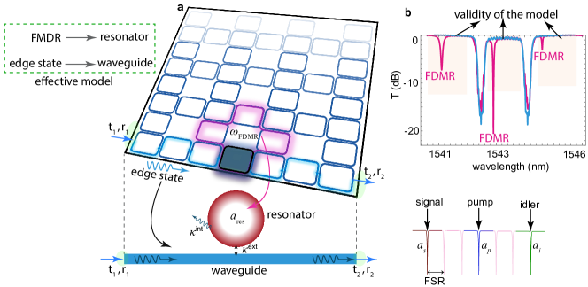
Figure 7: a The coupling between the FDMR and edge state can be represented as a single ring resonator with a radius of R coupled to a trivial waveguide. In this representation, the FDMR functions as a single-mode resonator with a resonance frequency $\omega_{\text{FDMR}}$, an annihilation operator $a_{\text{res}}$, and a Free-Spectral-Range (FSR). To initiate SFWM in this configuration, the system is pumped at mode $a_{p}$, resulting in the generation of photon pairs at the idler $a_{i}$ and signal $a_{s}$ modes, distributed above and below the pump mode. The input and output light undergo reflection and transmission at the facets of the waveguide with parameters $t_{i}$ and $r_{i}$. b The output of the FDMR indicates the regions where the effective resonator-waveguide model remains valid.

$$-i\omega a_{s} = -(i\omega_{s}+\frac{\kappa_{s}}{2})a_{s}+iGa_{i}^{\dagger}+\sqrt{\kappa_{s}^{\text{ext}}}a_{s}^{\text{ext}}+\sqrt{\kappa_{s}^{\text{int}}}a_{s}^{\text{int}},$$ (16)

$$-i\omega a_{i} = -(i\omega_{i}+\frac{\kappa_{i}}{2})a_{i}+iGa_{s}^{\dagger}+\sqrt{\kappa_{i}^{\text{ext}}}a_{i}^{\text{ext}}+\sqrt{\kappa_{i}^{\text{int}}}a_{i}^{\text{int}},$$ (17)

where $G=g_{\text{nl}}|\alpha_{p}|^{2}$ describes the effective nonlinear coupling between idler and signal. These coupled equations can be solved

$$\textbf{a}=\textbf{M}.\textbf{a}_{\textbf{in}}^{\text{ext}}+\textbf{N}.\textbf{a}_{\textbf{in}}^{\text{int}},$$ (18)

where $\textbf{a}=[a_{s},a_{i}^{\dagger}]^{\text{T}}$, $\textbf{a}_{\textbf{in}}^{\text{ext/int}}=[a_{s}^{\text{ext/int}},(a_{i}^{\text{ext/int}})^{\dagger}]^{\text{T}}$ with T stands for the transpose of the matrix, and

$$\textbf{M}(\omega)=\begin{pmatrix}\frac{\sqrt{\kappa_{s}^{\text{ext}}}\chi_{i}^{*}}{\chi_{s}\chi_{i}^{*}-G^{2}}&\frac{iG\sqrt{\kappa_{i}^{\text{ext}}}}{\chi_{s}\chi_{i}^{*}-G^{2}}\\ -\frac{iG\sqrt{\kappa_{s}^{\text{ext}}}}{\chi_{s}\chi_{i}^{*}-G^{2}}&\frac{\sqrt{\kappa_{i}^{\text{ext}}}\chi_{s}}{\chi_{s}\chi_{i}^{*}-G^{2}}\end{pmatrix},\\ \textbf{N}(\omega)=\begin{pmatrix}\frac{\sqrt{\kappa_{s}^{\text{int}}}\chi_{i}^{*}}{\chi_{s}\chi_{i}^{*}-G^{2}}&\frac{iG\sqrt{\kappa_{i}^{\text{int}}}}{\chi_{s}\chi_{i}^{*}-G^{2}}\\ -\frac{iG\sqrt{\kappa_{s}^{\text{int}}}}{\chi_{s}\chi_{i}^{*}-G^{2}}&\frac{\sqrt{\kappa_{i}^{\text{int}}}\chi_{s}}{\chi_{s}\chi_{i}^{*}-G^{2}}\end{pmatrix},$$ (19)

where $\chi_{j}(\omega)=\big{[}-i(\omega-\omega_{j})+\kappa_{j}/2\big{]}$ is the inverse of the field susceptibility with $\chi_{j}^{*}=\chi_{j}^{*}(-\omega)$. Since we are interested in the state of the output fields in the current system, we can rewrite the Eq. (18) in terms of the output fields using the input-output theory $a_{j,\text{in}}^{\text{ext/int}}=a_{j,\text{out}}^{\text{ext/int}}+\sqrt{\kappa_{j}^{\text{ext/int}}}a_{j}$ with $j=s,i$, resulting in

$$\textbf{a}=\textbf{M}.\textbf{a}_{\textbf{out}}^{\text{ext}}+\textbf{N}.\textbf{a}_{\textbf{out}}^{\text{int}}+\textbf{B}.\textbf{a},$$ (20)

where

$$\textbf{B}=\begin{pmatrix}\frac{\kappa_{s}\chi_{i}^{*}}{\chi_{s}\chi_{i}^{*}-G^{2}}&\frac{iG\kappa_{i}^{\text{ext}}}{\chi_{s}\chi_{i}^{*}-G^{2}}\\ -\frac{iG\kappa_{s}^{\text{ext}}}{\chi_{s}\chi_{i}^{*}-G^{2}}&\frac{\kappa_{i}^{\text{ext}}\chi_{s}}{\chi_{s}\chi_{i}^{*}-G^{2}}\end{pmatrix},$$ (21)

Note that the final term in this equation introduces reliance on the higher order of the output field operators $O([\textbf{a}_{\textbf{out}}^{\text{ext/int}}]^{n})$. However, for our analysis, we will disregard this term as our focus is solely on the generation of photon pairs.

The state of photons within the FDMR loop can be determined using the time-dependent Hamiltonian given by $|\psi\rangle=\mathcal{T}e^{-i/\hbar\int_{0}^{t}dtH(t)}|\psi(0)\rangle$, where $\mathcal{T}$ denotes the time order operator and $|\psi(0)\rangle=|0\rangle_{s,i}|0\rangle_{\mathrm{env}}$ represents the initial state of the idler, signal, and environment. Here, all modes are initially in the vacuum state, and hence, we have $a^{\text{ext}}_{s/i}|0\rangle_{s/i}=a^{\text{int}}_{\text{s/i}}|0\rangle_{env}=0$. For weak driving fields, the two-photon state can be simplified

$$|\psi\rangle\simeq\Big{[}1-\frac{i}{\hbar}\int_{0}^{t}dtH(t)\Big{]}|\psi(0)\rangle=\Big{[}1-i\int_{0}^{t}dt\big{(}g_{\text{nl}}a_{p}^{2}a_{s}^{\dagger}a_{i}^{\dagger}+h.c)\Big{]}|\psi(0)\rangle,$$ (22)

where we only considered the nonlinear part of the Hamiltonian. Utilizing the frequency domain representation of the operators

$$O(t)=\frac{1}{\sqrt{2\pi}}\int d\omega e^{-i\omega t}O(\omega),$$ (23)

we get

$$|\psi\rangle=\Big{[}1-\frac{ig_{\text{nl}}}{(2\pi)^{3/2}}\int_{0}^{t}dt\int d\omega d\omega^{\prime}\omega^{\prime\prime}\Big{(}a_{p}(\omega)^{2}a_{s}^{\dagger}(\omega^{\prime})a_{i}^{\dagger}(\omega^{\prime\prime})e^{-i(2\omega-\omega^{\prime}-\omega^{\prime\prime})t}+h.c\Big{)}\Big{]}|\psi(0)\rangle,$$ (24)

Replacing the pump drive with its classical form $a_{p}(\omega)\rightarrow|\alpha_{p}(\omega)|\delta(\omega_{p})$ and perform the time integral, results in

$$|\psi\rangle =\Big{[}1-\frac{ig_{\text{nl}}}{2\pi}\int d\omega^{\prime}d\omega^{\prime\prime}\Big{(}|\alpha_{p}(\omega_{p})|^{2}a_{s}^{\dagger}(\omega^{\prime})a_{i}^{\dagger}(\omega^{\prime\prime})+h.c\Big{)}\delta(2\omega_{p}-\omega^{\prime}-\omega^{\prime\prime})\Big{]}|\psi(0)\rangle$$ (25)

$$=\Big{[}1-\frac{iG}{2\pi}\int d\omega\Big{(}a_{s}^{\dagger}(\omega)a_{i}^{\dagger}(2\omega_{p}-\omega)+h.c\Big{)}\Big{]}|\psi(0)\rangle,$$ (26)

where the term $\delta(2\omega_{p}-\omega^{\prime}-\omega^{\prime\prime})$ fullfiles the phase matching condition $2\omega_{p}=\omega_{s}+\omega_{i}$ required for SFWM. The output state $|\psi\rangle_{\mathrm{out}}$ can be obtained by substituting $a_{s/i}$ with $a_{s/i}^{\text{out}}$ using Eq. (18)

$$|\psi\rangle_{\text{out}} =\int\frac{d\omega}{2\pi}\Big{[}\zeta_{00}(\omega)|0\rangle_{s,i}|0\rangle_{\text{env}}-\zeta_{11}(\omega)|1_{\omega},1_{2\omega_{p}-\omega}\rangle_{s,i}|0\rangle_{\text{env}}-\zeta_{10}(\omega)|1_{\omega},0\rangle_{s,i}|0,1_{2\omega_{p}-\omega}\rangle_{\text{env}}$$

$$-\zeta_{01}(\omega)|0,1_{2\omega_{p}-\omega}\rangle_{s,i}|1_{\omega},0\rangle_{\text{env}}-\eta(\omega)|0\rangle_{s,i}|1_{\omega},1_{2\omega_{p}-\omega}\rangle_{\text{env}}\Big{]},$$

with

$$\zeta_{00}(\omega) = 2\pi\delta(\omega)-iG\big{[}M_{12}^{*}(\omega)M_{22}(2\omega_{p}-\omega)+N_{12}^{*}(\omega)N_{22}(2\omega_{p}-\omega)$$

$$+ M_{11}(\omega)M_{21}^{*}(2\omega_{p}-\omega)+N_{11}(\omega)N_{21}^{*}(2\omega_{p}-\omega)\big{]},$$

$$\zeta_{11}(\omega) = iG\big{[}M_{11}^{*}(\omega)M_{22}(2\omega_{p}-\omega)+M_{12}(\omega)M_{21}^{*}(2\omega_{p}-\omega)\big{]},$$

$$\zeta_{10}(\omega) = iG\big{[}M_{11}^{*}(\omega)N_{22}(2\omega_{p}-\omega)+N_{12}(\omega)M_{21}^{*}(2\omega_{p}-\omega)\big{]},$$ (28)

$$\zeta_{01}(\omega) = iG\big{[}N_{11}^{*}(\omega)M_{22}(2\omega_{p}-\omega)+M_{12}(\omega)N_{21}^{*}(2\omega_{p}-\omega)\big{]},$$

$$\eta(\omega) = iG\big{[}N_{11}^{*}(\omega)N_{22}(2\omega_{p}-\omega)+N_{12}(\omega)N_{21}^{*}(2\omega_{p}-\omega)\big{]},$$

In Eq. (.2), the initial term represents the presence of signal and idler in a vacuum state. The subsequent component characterizes the idler-signal two-photon states, giving rise to coincidences between the idler and signal modes. The third and fourth terms correspond to situations where one photon is present in either the idler or signal mode. This occurrence arises due to the loss of an idler or signal photon, and these terms contribute to the single count rates. Finally, the last term illustrates the loss of the generated photons to the surrounding environment. The parameters $|\zeta_{ij}(\omega)|^{2}$ and $|\eta(\omega)|^{2}$ quantify the probability of each of these described events. Based on this, the photon-pair generation rate is expressed as [56, 55, 57]

$$N_{c}=\int_{-\infty}^{\infty}d\omega|\zeta_{11}(\omega)|^{2}=G^{2}\int_{-\infty}^{\infty}d\omega\Big{|}M_{11}^{*}(\omega)M_{22}(2\omega_{p}-\omega)+M_{12}(\omega)M_{21}^{*}(2\omega_{p}-\omega)\Big{|}^{2}.$$ (29)

The second term of the above equation $M_{12}M_{21}^{*}\propto G^{2}$ represents a higher order pump-dependent correction of the coincidence. In the weak pumping regime $G^{2}\ll\kappa_{s}\kappa_{i}$ we can simplify the above equation

$$N_{c}\approx G^{2}\int_{-\infty}^{\infty}d\omega|M_{11}(\omega)|^{2}|M_{22}(2\omega_{p}-\omega)|^{2}\approx G^{2}\int_{-\infty}^{\infty}d\omega\Big{[}\frac{\kappa_{s}^{\text{ext}}}{(\omega-\omega_{s})^{2}+\kappa_{s}^{2}/4}\Big{]}\times\Big{[}\frac{\kappa_{i}^{\text{ext}}}{(2\omega_{p}-\omega-\omega_{i})^{2}+\kappa_{i}^{2}/4}\Big{]}.$$ (30)

We now can perform the frequency integral and find an analytical expression for the coincidence rate

$$N_{c}\approx\frac{8\pi G^{2}(\kappa_{s}^{\text{ext}}\kappa_{i}^{\text{ext}})(\kappa_{s}+\kappa_{i})}{\kappa_{s}\kappa_{i}\Big{[}(\kappa_{s}+\kappa_{i})^{2}+(2\omega_{p}-\omega_{s}-\omega_{i})\Big{]}},$$ (31)

Considering the phase matching condition $2\omega_{p}=\omega_{s}+\omega_{i}$ we find

$$N_{c}=\frac{8\pi G^{2}(\kappa_{s}^{\text{ext}}\kappa_{i}^{\text{ext}})}{\kappa_{s}\kappa_{i}(\kappa_{s}+\kappa_{i})}=\frac{8\pi g_{\text{nl}}^{2}P^{2}}{(\hbar\omega_{p})^{2}(\kappa_{s}+\kappa_{i})}\Big{(}\frac{\kappa_{s}^{\text{ext}}}{\kappa_{s}}\Big{)}\Big{(}\frac{\kappa_{i}^{\text{ext}}}{\kappa_{i}}\Big{)}\Big{(}\frac{\kappa_{p}^{\text{ext}}}{\kappa_{p}^{2}}\Big{)}^{2},$$ (32)

In the symmetric coupling rates $\kappa=\kappa_{s}=\kappa_{i}=\kappa_{p}$ and critical coupling regime $\kappa_{j}^{\text{ext}}/\kappa_{j}=1/2$ the above equation reduces to

$$N_{c}=\frac{\pi g_{\text{nl}}^{2}P^{2}}{4(\hbar\omega_{p})^{2}\kappa^{3}},$$ (33)

as reported in the main text. In reality, the measured coincidence rate deviates from this equation and is influenced by the detection efficiency and losses in the measurement chain, leading to the modified expression $N_{\text{tot},c}=\eta_{i}\eta_{s}N_{c}$.

The single-count rates for the idler and signal can be expressed as follows

$$N_{s}=\int_{-\infty}^{\infty}d\omega|\zeta_{10}(\omega)|^{2} \approx\frac{8\pi g_{\text{nl}}^{2}P^{2}}{(\hbar\omega_{p})^{2}(\kappa_{s}+\kappa_{i})}\Big{(}\frac{\kappa_{s}^{\text{ext}}}{\kappa_{s}}\Big{)}\Big{(}\frac{\kappa_{i}^{\text{int}}}{\kappa_{i}}\Big{)}\Big{(}\frac{\kappa_{p}^{\text{ext}}}{\kappa_{p}^{2}}\Big{)}^{2},$$ (34)

$$N_{i}=\int_{-\infty}^{\infty}d\omega|\zeta_{01}(\omega)|^{2} \approx\frac{8\pi g_{\text{nl}}^{2}P^{2}}{(\hbar\omega_{p})^{2}(\kappa_{s}+\kappa_{i})}\Big{(}\frac{\kappa_{s}^{\text{int}}}{\kappa_{s}}\Big{)}\Big{(}\frac{\kappa_{i}^{\text{ext}}}{\kappa_{i}}\Big{)}\Big{(}\frac{\kappa_{p}^{\text{ext}}}{\kappa_{p}^{2}}\Big{)}^{2},$$ (35)

Note that, the leakage/residue of the pump, the efficiency of the measurement chain $\eta_{j}$, and the dark counts $D_{j}$ of the photodetectors add extra terms to the single-count rates

$$N_{\text{tot},j}=\eta_{j}N_{j}+N_{j,p}+D_{j},$$ (36)

with $j=s,i$ and as described in the Methods. Note that, the additional noise photons arising from the pump leakage $N_{j,p}=\beta_{j}P$ shows a linear dependency to the pump power $P$ [58, 59]. The coefficient $\beta_{j}$ is affected by imperfections in the bandpass filter and the presence of laser sidebands. These imperfections enable pump photons to reach the photodetectors, leading to an overall increase in the total single counts integrated over the measurement time.

.3 Phase detuning calibration

The spectral width of each bandgap is 1.28nm on average in the wavelength region of interest plotted in Fig. 2b. The FDMR are, on average, detuned 0.92nm from the short-wavelength edge of their respective bandgaps. This equates to 73.4% of the way across each bandgap, or a phase detune of approximately 1.47$\pi$.

.4 Power transmission spectral

In this section, we analyze the transmission spectrum of the FDMR, considering the single-mode Kerr nonlinearity, as depicted in the effective resonator-waveguide representation shown in Fig. 7a. To start, we set $a_{\text{res}}=a_{p}=a_{s}=a_{i}$ in the Hamiltonian (13). This allows us to derive the Hamiltonian that describes the single-mode Kerr nonlinearity and its role in the transmission behavior of the nonlinear FDMR

$$H=\hbar\omega_{\text{FDMR}}a_{\text{res}}^{\dagger}a_{\text{res}}-\hbar g_{\text{nl}}a_{\text{res}}^{\dagger 2}a_{\text{res}}^{2},$$ (37)

The equation of motion describing the dynamics of the system then is given by

$$\dot{a}_{\text{res}}=-\Big{(}i\big{[}\omega_{\text{FDMR}}-2g_{\text{nl}}a_{\text{res}}^{\dagger}a_{\text{res}}\big{]}+\frac{\kappa}{2}\Big{)}a_{\text{res}}+\sqrt{\kappa^{\text{ext}}}a^{\text{ext}}+\sqrt{\kappa^{\text{int}}}a^{\text{int}},$$ (38)

where $\kappa=\kappa^{\text{ext}}+\kappa^{\text{int}}$, with $\kappa^{\text{ext}}$ and $\kappa^{\text{int}}$ represent the extrinsic and intrinsic coupling rates, respectively. Furthermore, $a^{\text{ext}}$ and $a^{\text{int}}$ are the annihilation operators of the input field from the edge state and loss channels, respectively. In the frequency domain, we can solve the coherent response of Eq. (38), leading to

$$\langle a_{\text{res}}(\omega)\rangle=\frac{\sqrt{\kappa^{\text{ext}}}\langle a^{\text{ext}}(\omega)\rangle}{\kappa/2-i\Big{(}\omega-\omega_{\text{FDMR}}+2g_{\text{nl}}\langle a_{\text{res}}^{\dagger}a_{\text{res}}\rangle\Big{)}},$$ (39)

here we consider $\langle a^{\text{int}}\rangle=0$. Using the input-output theory $a_{\text{out}}=a^{\text{ext}}-\sqrt{\kappa^{\text{ext}}}a_{\text{res}}$ we can find the coherent transmission of the system

$$T_{0}(\omega)=\frac{\langle a_{\text{out}}(\omega)\rangle}{\langle a_{\text{ext}}(\omega)\rangle}=1-\frac{\kappa^{\text{ext}}}{\kappa/2-i\Big{(}\omega-\omega_{\text{FDMR}}+2g_{\text{nl}}n_{\text{res}}\Big{)}}$$ (40)

which has a nonlinear dependency to the photons inside the cavity $n_{\text{res}}=\langle a_{\text{res}}^{\dagger}a_{\text{res}}\rangle$, as expected for a cavity-based Kerr nonlinear platforms. In the low-power regime, the nonlinear term $2g_{\text{nl}}$ in the equation becomes negligible, and the transmission function $T_{0}$ follows the standard Lorentzian function of a cavity.

The Total transmission of the system is affected by several factors, which include the reflection and transmission at the input ($r_{1},t_{1}$) and output ($r_{2},t_{2}$) facets of the waveguide, as well as the coupling to and from the edge state. By taking these reflection and transmission parameters into account, we can determine the normalized power transmission at the output of the lensed coupled waveguide facet [60]

$$T(\omega)=\frac{|t_{1}t_{2}|^{2}|T_{0}(\omega)|^{2}}{\Big{|}1-r_{1}r_{2}T_{0}(\omega)^{2}e^{-i\phi}\Big{|}^{2}},$$ (41)

where $\phi$ represents the propagation phase of light in the coupling waveguide and edge state, which depends on the resonance frequency and propagation length. To fit the transmission spectrum of the FDMR, as shown in Fig. 2d of the main text, we used Eq. (41).

Idler				Signal
FSR	$Q_{t}$	$Q_{e}$	$Q_{i}$	$Q_{t}$	$Q_{e}$	$Q_{i}$
1	62918	95050	186120	25471	30966	143542
2	30806	122399	41167	47116	124749	75712
3	47184	82361	110472	52778	83187	144382
4	62374	95585	179523	21536	108772	26852
5	33550	50157	101326	33174	51111	94531
6	54625	88776	142001	51767	78703	151259
7	75958	227300	114081	20122	113791	24445
8	36358	60597	90891	28535	43627	82483
9	46185	74315	122014	39249	61741	107736

Table 2: The extracted values for total $Q_{t}$, extrinsic $Q_{e}$ and intrinsic $Q_{i}$ quality factors for nine FDMR modes.

.5 Second-order correlation function for FDMR

Figure 8 reports the raw data of the second-order cross-correlation function $g^{(2)}_{si}$ and auto-correlation functions of the idler and signal $g^{(2)}_{ss}$ and $g^{(2)}_{ii}$ for different pump powers at the presence of the FDMR. The result indicates the violation of the Cauchy-Schwarz inequality $[g^{(2)}_{si}(t)]^{2}\leq g^{(2)}_{ss}(t)\times g^{(2)}_{ii}(t)$ at time $t=0$.

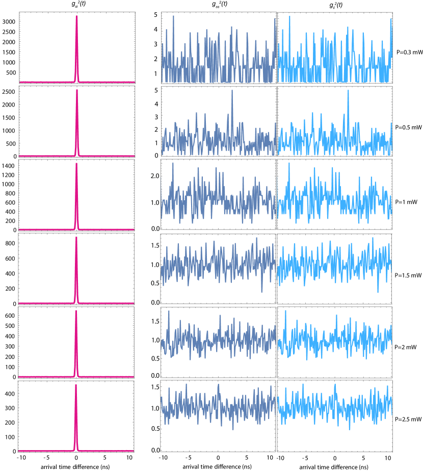
Figure 8: Comparing time-dependent the second-order cross-correlation function $g^{(2)}_{si}(t)$ and auto-correlation functions of the idler and signal $g^{(2)}_{ss}(t)$ and $g^{(2)}_{ii}(t)$ for different pump powers at the presence of the FDMR.

.6 Coincidence rate: FDMR versus edge state

In this section, we present the raw data of the measured coincidence counts of the FDMR and edge state, including the detection efficiency and setup loss without calibration i.e. $N_{\text{tot},c}=\eta_{i}\eta_{s}N_{c}$, as described in the Methods. Due to the small size of our sample and the low efficiency of photon conversion in SFWM, the edge state cannot generate significant photon pairs in the system. This limitation is attributed to the short interaction time available for generating pair-correlated photons in the edge state, which is considerably smaller compared to the resonance condition.

As we increase the power of the laser, noise and pump leakage to the photodetector become prominent. Therefore, no substantial coincidences have been observed in the edge state for various laser powers. In contrast, when the FDMR is activated, a significant level of coincidence has been detected. Figure 9 illustrates that the noise level increases as the laser power is raised.

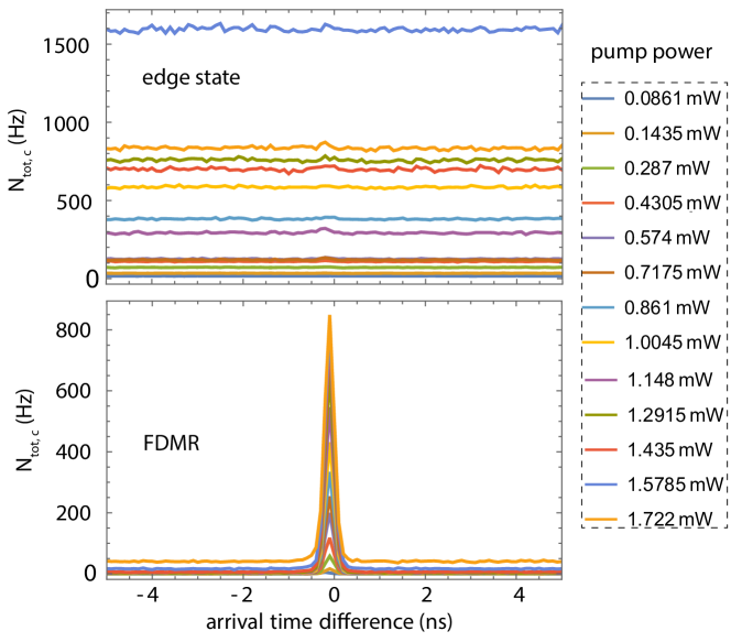
Figure 9: The measured (uncalibrated) coincidence rate of the edge state and the FDMR as a function of arrival time at different pump powers.

.7 Phase detune calibration

To calibrate the heating power used in our experiment and to find its relation with the applied phase detune, $\Delta\phi$, we tuned the heating power from 7 to 27 mW and we measured the wavelength of the excited FDMR shown in Fig. 10a. In addition, we simulated the transmission spectrum of the lattice and we plotted the wavelength of the FDMR for the phase detuning of $\Delta\phi=1.5\pi$ to $2.65\pi$ applied to an entire micoring at the boundary of the lattice, Fig. 10b. The simulation and experimental results show that the wavelength of FDMR is linearly shifted by increasing the phase detune and heating power. By comparing the simulation and experiment, we obtained the $\Delta\phi=2.37\pi$ for excitation of the FDMR at the wavelength of 1545.265 nm.

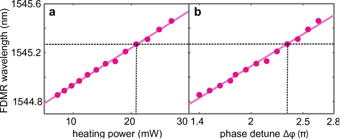
Figure 10: a and b,) Phase detune calibration using plots FDMR wavelength versus heating power and $\Delta\phi$.

References

- [1] Horodecki, R., Horodecki, P., Horodecki, M. & Horodecki, K. Quantum entanglement. Rev. Mod. Phys. 81, 865–942 (2009). URL https://link.aps.org/doi/10.1103/RevModPhys.81.865.
- [2] Gisin, N. Quantum chance: Nonlocality, teleportation and other quantum marvels (Springer, 2014).
- [3] Aslam, N. et al. Quantum sensors for biomedical applications. Nature Reviews Physics 5, 157–169 (2023). URL https://doi.org/10.1038/s42254-023-00558-3.
- [4] Pirandola, S., Bardhan, B. R., Gehring, T., Weedbrook, C. & Lloyd, S. Advances in photonic quantum sensing. Nature Photonics 12, 724–733 (2018). URL https://doi.org/10.1038/s41566-018-0301-6.
- [5] Ladd, T. D. et al. Quantum computers. Nature 464, 45–53 (2010). URL https://doi.org/10.1038/nature08812.
- [6] Harrow, A. W. & Montanaro, A. Quantum computational supremacy. Nature 549, 203–209 (2017). URL https://doi.org/10.1038/nature23458.
- [7] Couteau, C. et al. Applications of single photons to quantum communication and computing. Nature Reviews Physics 1–13 (2023).
- [8] Wehner, S., Elkouss, D. & Hanson, R. Quantum internet: A vision for the road ahead. Science 362, eaam9288 (2018). URL https://www.science.org/doi/abs/10.1126/science.aam9288. eprint https://www.science.org/doi/pdf/10.1126/science.aam9288.
- [9] Wang, J., Sciarrino, F., Laing, A. & Thompson, M. G. Integrated photonic quantum technologies. Nature Photonics 14, 273–284 (2020). URL https://doi.org/10.1038/s41566-019-0532-1.
- [10] Pelucchi, E. et al. The potential and global outlook of integrated photonics for quantum technologies. Nature Reviews Physics 4, 194–208 (2022). URL https://doi.org/10.1038/s42254-021-00398-z.
- [11] Kues, M. et al. On-chip generation of high-dimensional entangled quantum states and their coherent control. Nature 546, 622–626 (2017).
- [12] Shadbolt, P. J. et al. Generating, manipulating and measuring entanglement and mixture with a reconfigurable photonic circuit. Nature Photonics 6, 45–49 (2012).
- [13] Matthews, J. C., Politi, A., Bonneau, D. & O’Brien, J. L. Heralding two-photon and four-photon path entanglement on a chip. Physical review letters 107, 163602 (2011).
- [14] Lu, X. et al. Chip-integrated visible–telecom entangled photon pair source for quantum communication. Nature Physics 15, 373–381 (2019). URL https://doi.org/10.1038/s41567-018-0394-3.
- [15] Topolancik, J., Ilic, B. & Vollmer, F. Experimental observation of strong photon localization in disordered photonic crystal waveguides. Phys. Rev. Lett. 99, 253901 (2007). URL https://link.aps.org/doi/10.1103/PhysRevLett.99.253901.
- [16] Sapienza, L. et al. Cavity quantum electrodynamics with anderson-localized modes. Science 327, 1352–1355 (2010). URL https://www.science.org/doi/abs/10.1126/science.1185080. eprint https://www.science.org/doi/pdf/10.1126/science.1185080.
- [17] Metcalf, B. J. et al. Quantum teleportation on a photonic chip. Nature Photonics 8, 770–774 (2014). URL https://doi.org/10.1038/nphoton.2014.217.
- [18] Burgwal, R. et al. Using an imperfect photonic network to implement random unitaries. Opt. Express 25, 28236–28245 (2017). URL https://opg.optica.org/oe/abstract.cfm?URI=oe-25-23-28236.
- [19] Lu, L., Joannopoulos, J. D. & Soljačić, M. Topological photonics. Nature photonics 8, 821–829 (2014).
- [20] Khanikaev, A. B. & Shvets, G. Two-dimensional topological photonics. Nat. photonics 11, 763–773 (2017).
- [21] Ozawa, T. et al. Topological photonics. Rev. Mod. Phys. 91, 015006 (2019).
- [22] Bandres, M. A. et al. Topological insulator laser: Experiments. Science 359, eaar4005 (2018). URL https://www.science.org/doi/abs/10.1126/science.aar4005. eprint https://www.science.org/doi/pdf/10.1126/science.aar4005.
- [23] St-Jean, P. et al. Lasing in topological edge states of a one-dimensional lattice. Nat. Photonics 11, 651–656 (2017).
- [24] Bahari, B. et al. Nonreciprocal lasing in topological cavities of arbitrary geometries. Science 358, 636–640 (2017).
- [25] Kirsch, M. S. et al. Nonlinear second-order photonic topological insulators. Nature Physics 17, 995–1000 (2021). URL https://doi.org/10.1038/s41567-021-01275-3.
- [26] Mukherjee, S. & Rechtsman, M. C. Observation of floquet solitons in a topological bandgap. Science 368, 856–859 (2020).
- [27] Mittal, S., Moille, G., Srinivasan, K., Chembo, Y. K. & Hafezi, M. Topological frequency combs and nested temporal solitons. Nature Physics 17, 1169–1176 (2021). URL https://doi.org/10.1038/s41567-021-01302-3.
- [28] Rechtsman, M. C. et al. Topological protection of photonic path entanglement. Optica 3, 925–930 (2016).
- [29] Barik, S. et al. A topological quantum optics interface. Science 359, 666–668 (2018). URL https://www.science.org/doi/abs/10.1126/science.aaq0327. eprint https://www.science.org/doi/pdf/10.1126/science.aaq0327.
- [30] Segev, M. & Bandres, M. A. Topological photonics: Where do we go from here? Nanophotonics 10, 425–434 (2020).
- [31] Blanco-Redondo, A., Bell, B., Oren, D., Eggleton, B. J. & Segev, M. Topological protection of biphoton states. Science 362, 568–571 (2018). URL https://www.science.org/doi/abs/10.1126/science.aau4296. eprint https://www.science.org/doi/pdf/10.1126/science.aau4296.
- [32] Mittal, S., Goldschmidt, E. A. & Hafezi, M. A topological source of quantum light. Nature 561, 502–506 (2018).
- [33] Mittal, S., Orre, V. V., Goldschmidt, E. A. & Hafezi, M. Tunable quantum interference using a topological source of indistinguishable photon pairs. Nature Photonics 15, 542–548 (2021). URL https://doi.org/10.1038/s41566-021-00810-1.
- [34] Dai, T. et al. Topologically protected quantum entanglement emitters. Nature Photonics 16, 248–257 (2022). URL https://doi.org/10.1038/s41566-021-00944-2.
- [35] Kumar, R., Ong, J. R., Recchio, J., Srinivasan, K. & Mookherjea, S. Spectrally multiplexed and tunable-wavelength photon pairs at 1.55 μm from a silicon coupled-resonator optical waveguide. Opt. Lett. 38, 2969–2971 (2013). URL https://opg.optica.org/ol/abstract.cfm?URI=ol-38-16-2969.
- [36] Ma, C. et al. Silicon photonic entangled photon-pair and heralded single photon generation with car¿ 12,000 and g (2)(0)¡ 0.006. Optics Express 25, 32995–33006 (2017).
- [37] Ma, Z. et al. Ultrabright quantum photon sources on chip. Physical Review Letters 125, 263602 (2020).
- [38] Afifi, A. E. et al. Contra-directional pump reject filters integrated with a micro-ring resonator photon-pair source in silicon. Optics Express 29, 25173–25188 (2021).
- [39] Guo, K. et al. Nonclassical optical bistability and resonance-locked regime of photon-pair sources using silicon microring resonator. Physical Review Applied 11, 034007 (2019).
- [40] Clementi, M. et al. Programmable frequency-bin quantum states in a nano-engineered silicon device. Nature Communications 14, 176 (2023).
- [41] Afzal, S. & Van, V. Trapping light in a floquet topological photonic insulator by floquet defect mode resonance. APL Photonics 6 (2021).
- [42] Kues, M. et al. On-chip generation of high-dimensional entangled quantum states and their coherent control. Nature 546, 622–626 (2017). URL https://doi.org/10.1038/nature22986.
- [43] Imany, P. et al. High-dimensional optical quantum logic in large operational spaces. npj Quantum Information 5, 59 (2019). URL https://doi.org/10.1038/s41534-019-0173-8.
- [44] Zimmerling, T. J., Afzal, S. & Van, V. Broadband resonance-enhanced frequency generation by four-wave mixing in a silicon floquet topological photonic insulator. APL Photonics 7 (2022).
- [45] Afzal, S. & Van, V. Topological phases and the bulk-edge correspondence in 2D photonic microring resonator lattices. Opt. Express 26, 14567–14577 (2018). URL http://www.opticsexpress.org/abstract.cfm?URI=oe-26-11-14567.
- [46] Liang, G. Q. & Chong, Y. D. Optical resonator analog of a two-dimensional topological insulator. Physical Review Letters 110, 203904 (2013).
- [47] Gao, X. et al. Dirac-vortex topological cavities. Nat. Nanotechnol. 15, 1012–1018 (2020).
- [48] Shao, Z.-K. et al. A high-performance topological bulk laser based on band-inversion-induced reflection. Nat. Nanotechnol. 15, 67–72 (2020).
- [49] Santiago-Cruz, T. et al. Resonant metasurfaces for generating complex quantum states. Science (New York, N.Y.) 377, 991—995 (2022). URL https://doi.org/10.1126/science.abq8684.
- [50] Caspani, L. et al. Integrated sources of photon quantum states based on nonlinear optics. Light: Science & Applications 6, e17100–e17100 (2017). URL https://doi.org/10.1038/lsa.2017.100.
- [51] Tsay, A. & Van, V. Analytic theory of strongly-coupled microring resonators. IEEE Journal of Quantum Electronics 47, 997–1005 (2011).
- [52] Cui, C., Zhang, L. & Fan, L. In situ control of effective kerr nonlinearity with pockels integrated photonics. Nature Physics 18, 497–501 (2022). URL https://doi.org/10.1038/s41567-022-01542-x.
- [53] Barzanjeh, S., Abdi, M., Milburn, G. J., Tombesi, P. & Vitali, D. Reversible optical-to-microwave quantum interface. Phys. Rev. Lett. 109, 130503 (2012). URL https://link.aps.org/doi/10.1103/PhysRevLett.109.130503.
- [54] Arnold, G. et al. Converting microwave and telecom photons with a silicon photonic nanomechanical interface. Nature Communications 11, 4460 (2020). URL https://doi.org/10.1038/s41467-020-18269-z.
- [55] Helt, L. G., Yang, Z., Liscidini, M. & Sipe, J. E. Spontaneous four-wave mixing in microring resonators. Optics letters 35, 3006–3008 (2010).
- [56] Bajoni, D. et al. Micrometer-scale integrated silicon source of time-energy entangled photons. Optica 2, 88–94 (2015). URL https://opg.optica.org/viewmedia.cfm?uri=optica-2-2-88&seq=0&html=truehttps://opg.optica.org/abstract.cfm?uri=optica-2-2-88https://opg.optica.org/optica/abstract.cfm?uri=optica-2-2-88.
- [57] Helt, L. G., Liscidini, M. & Sipe, J. E. How does it scale? comparing quantum and classical nonlinear optical processes in integrated devices. JOSA B 29, 2199–2212 (2012).
- [58] Clemmen, S. et al. Continuous wave photon pair generation in silicon-on-insulator waveguides and ring resonators. Optics Express 17, 16558–16570 (2009). URL https://opg.optica.org/viewmedia.cfm?uri=oe-17-19-16558&seq=0&html=truehttps://opg.optica.org/abstract.cfm?uri=oe-17-19-16558%****␣main.tex␣Line␣800␣****https://opg.optica.org/oe/abstract.cfm?uri=oe-17-19-16558.
- [59] Engin, E. et al. Photon pair generation in a silicon micro-ring resonator with reverse bias enhancement. Opt. Express 21, 27826–27834 (2013). URL http://opg.optica.org/oe/abstract.cfm?URI=oe-21-23-27826.
- [60] Gao, M. et al. Probing material absorption and optical nonlinearity of integrated photonic materials. Nature Communications 13, 3323 (2022). URL https://doi.org/10.1038/s41467-022-30966-5.
Supplementary Materials