Two-loop form factors for diphoton production in quark annihilation channel with heavy quark mass dependence

Abstract

We present the computation of the two-loop form factors for diphoton production in the quark annihilation channel. These quantities are relevant for the NNLO QCD corrections to diphoton production at LHC recently presented in Becchetti:ta . The computation is performed retaining full dependence on the mass of the heavy quark in the loops. The master integrals are evaluated by means of differential equations which are solved exploiting the generalised power series technique.

LON³LO

IFIC/23-32

FTUV-23-0808.6381

1 Introduction

The production of photon pairs (diphotons) at the Large Hadron Collider (LHC) is a very relevant process for phenomenological studies in the context of the Standard Model (SM) ATLAS:2021mbt ; ATLAS:2017cvh ; CMS:2014mvm ; ATLAS:2012fgo and in the search for new physics ATLAS:2023hbp ; ATLAS:2023meo ; ATLAS:2022abz ; CMS:2019pov ; CMS:2016kgr ; ATLAS:2017ayi . In particular, diphoton final states are highly relevant for Higgs boson studies ATLAS:2022fnp ; CMS:2022wpo ; CMS:2021kom ; CMS:2020xrn ; ATLAS:2018hxb ; CMS:2014afl ; ATLAS:2014cnc ; ATLAS:2014yga (and played a crucial role in its discovery ATLAS:2012yve ; CMS:2012qbp ), as they constitute an irreducible background for a Higgs boson decaying into two photons.

Due to its physical relevance, the study of diphoton production requires dedicated and accurate theoretical calculations, in particular including QCD radiative corrections at high perturbative orders. The state of the art for diphoton production is represented by the next-to-next-to-leading order (NNLO) QCD corrections Catani:2011qz ; Campbell:2016yrh ; Catani:2018krb ; Schuermann:2022qdm to the Born subprocess (which proceeds via quark annihilation $q\bar{q}\rightarrow\gamma\gamma$). The relevant scattering amplitudes in the completely massless case have been known in the literature for some time Ametller:1985di ; Parke:1986gb ; Dicus:1987fk ; Barger:1989yd ; Mangano:1990by ; Bern:1994fz ; Signer:1995np ; Balazs:1997hv ; DelDuca:1999pa ; Anastasiou:2002zn ; DelDuca:2003uz .

More recently, scattering amplitudes belonging to higher orders in the strong coupling $\alpha_{s}$ (i.e. beyond the NNLO) have become available (in the massless case): the three-loop matrix element Caola:2022dfa ; the two-loop scattering amplitudes for a photon pair in association with one jet in the leading colour approximation Chawdhry:2020for ; Agarwal:2021grm ; Chawdhry:2021mkw , and, very recently, the full colour case Agarwal:2021vdh . The two-loop scattering amplitudes for diphoton production in gluon fusion Bern:2001df together with the recent computation of diphoton production in association with one jet Chawdhry:2021hkp at NNLO emphasise that all the building blocks are in place for the next-to-next-to-next-to-leading order (N³LO) massless calculation. However, the implementation of slicing subtraction methods to reach the N³LO accuracy could be challenging in this case, due to the presence of a high number of particles in the final state and the use of a photon isolation prescription. More clearly, the NNLO calculation of the diphoton cross section in association with one jet at small diphoton transverse momentum could be very CPU demanding.

In the massive case, the first non-trivial corrections appear at the NNLO, through the inclusion of top quark loops and top quark radiation. The mass effects of the so-called box contribution ($gg\rightarrow\gamma\gamma$) were discussed in ref. Campbell:2016yrh (together with partial N³LO contributions). Due to the large gluon luminosity at the LHC, the size of the box contribution is of the order of the Born subprocess $q\bar{q}\rightarrow\gamma\gamma$. It is therefore of interest to calculate the corrections of the following perturbative order (i.e. N³LO contributions). Regarding the gluon fusion channel only, the simplest approach (which captures very sizable components) is to consider the NLO QCD corrections to the box contribution, since these form a gauge invariant subset Bern:2001df of the whole N³LO gluon fusion channel. In this context, two recent papers have shown the impact of these massive NLO QCD corrections on the gluon fusion channel Maltoni:2018zvp ; Chen:2019fla .

Considering the full NNLO accuracy, there are still three missing ingredients that were not available or not presented together in previous phenomenological studies in the literature: i) the massive one-loop real-virtual contribution ($q\bar{q}\rightarrow\gamma\gamma g$ and $q(\bar{q})g\rightarrow\gamma\gamma q(\bar{q})$), the double real radiation of top quarks ($q\bar{q}\rightarrow\gamma\gamma t\bar{t}$ and $gg\rightarrow\gamma\gamma t\bar{t}$) and the two-loop virtual corrections to the Born sub-process $q\bar{q}\rightarrow\gamma\gamma$.

In this paper we report on the computation of the two-loop form factors for diphoton production in the quark annihilation channel, where the full dependence on the heavy quark mass, which appear in the loops, is retained. This contribution is included in the recently presented phenomenological study of full massive NNLO QCD corrections to diphoton production Becchetti:ta .

The two-loop form factors have been computed employing standard techniques for scattering amplitude calculations. We considered the partonic process $q\bar{q}\to\gamma\gamma$ and the relative two-loop Feynman diagrams, which contain a massive heavy quark loop, as shown in figure 1. The associated amplitude is decomposed into a combination of tensors multiplied by scalar form factors, as described in Peraro:2020sfm , and the scalar integrals appearing in the expressions of the form factors are written in terms of a basis of master integrals (MIs). The decomposition in terms of MIs is performed using Identity-by-Parts (IBPs) relations Chetyrkin:1979bj ; Chetyrkin:1981qh , via the Laporta Algorithm Laporta:2001dd , implemented in the computer code KIRA Maierhofer:2017gsa ; Klappert:2020nbg .

The MIs relevant for this process have been computed by means of the differential equations method Kotikov:1990kg ; Kotikov:1991pm ; Bern:1993kr ; Remiddi:1997ny ; Gehrmann:1999as ; Argeri:2007up ; Henn:2013pwa ; Henn:2014qga . While the integrals associated to the planar topologies have already been studied in the literature Becchetti:2017abb ; Caron-Huot:2014lda ; Bonciani:2003te ; Aglietti:2004tq ; Bonciani:2003hc ; Bonciani:2007eh ; Bonciani:2008ep , a complete computation for the non-planar ones is still not available. Indeed, while the planar MIs admit an analytic solution in terms of Multiple Polylogarithmic functions (MPLs) Goncharov:2001iea ; Goncharov:1998kja ; Goncharov2001 ; Remiddi:1999ew ; Vollinga:2004sn ; Duhr:2019tlz , it is known that the functional space for the analytic solution of the non-planar double-box family Adams:2017tga contains elliptic integrals brown2013multiple ; Broedel:2014vla ; Broedel:2017kkb ; ManinModular ; Brown:mmv ; Adams:2014vja ; Frellesvig:2021hkr ; Frellesvig:2023iwr ; Gorges:2023zgv ; Duhr:2022pch ; Duhr:2022dxb ; Bourjaily:2022bwx . In recent years, a big effort has been devoted to the understanding of the analytic structure of Feynman integrals which do not admit an expression in terms of MPLs. However, even in the cases in which an analytic solution in closed form is available, the numerical evaluation of the functions associated to such solution can be extremely challenging for phenomenological applications Abreu:2022vei ; Abreu:2022cco .

In order to be able to overcome the issues previously described, we choose to exploit the generalised power series method Pozzorini:2005ff ; Aglietti:2007as ; Bonciani:2018uvv ; Lee:2017qql ; Mandal:2018cdj ; Moriello:2019yhu ; Bonciani:2019jyb to solve the systems of differential equations associated to the MIs. This technique, currently implemented in two public computer codes Hidding:2020ytt ; Armadillo:2022ugh , has recently attracted a lot of interest due to its wide range of applicability and it has been successfully employed in several phenomenological applications Becchetti:2020wof ; Bonciani:2021zzf ; Becchetti:ta ; Bonciani:2022jmb . Specifically, in the calculation reported in this paper, we used the software DiffExp Hidding:2020ytt to obtain a semi-analytic solution for the MIs.

The paper is organised as follows. In section 2, we describe the general setup for the computation and we set the context in which the two-loop form factors, presented in this paper, are relevant. We discuss the form factors computation along with their UV singularity structure and the renormalisation procedure. In section 3 instead we report on the MIs calculation. We describe the different integral families that appear in the computation and the approach that we used to solve the differential equations, along with a brief analysis on the geometry underlying the actual analytic solution.

Moreover, as ancillary material attached to this paper, we furnish the analytic expressions of the finite reminder for the form factors, alongside with Mathematica files which allows for a standalone evaluation of the MIs with DiffExp.

2 Computational setup and amplitude structure

In this paper, we consider the two-loop form factors for diphoton production in the quark annihilation channel with a heavy quark loop. At the partonic level, the scattering amplitude proceeds as the Born subprocess:

$$q(p_{1})+\overline{q}(p_{2})\rightarrow\gamma(p_{3})+\gamma(p_{4}).$$ (1)

The kinematics for this process is described by the Mandelstam variables

$$s=-(p_{1}+p_{2})^{2},\;t=-(p_{1}-p_{3})^{2},\;u=-(p_{2}-p_{3})^{2},\;\text{with}\;s+t+u=0,$$ (2)

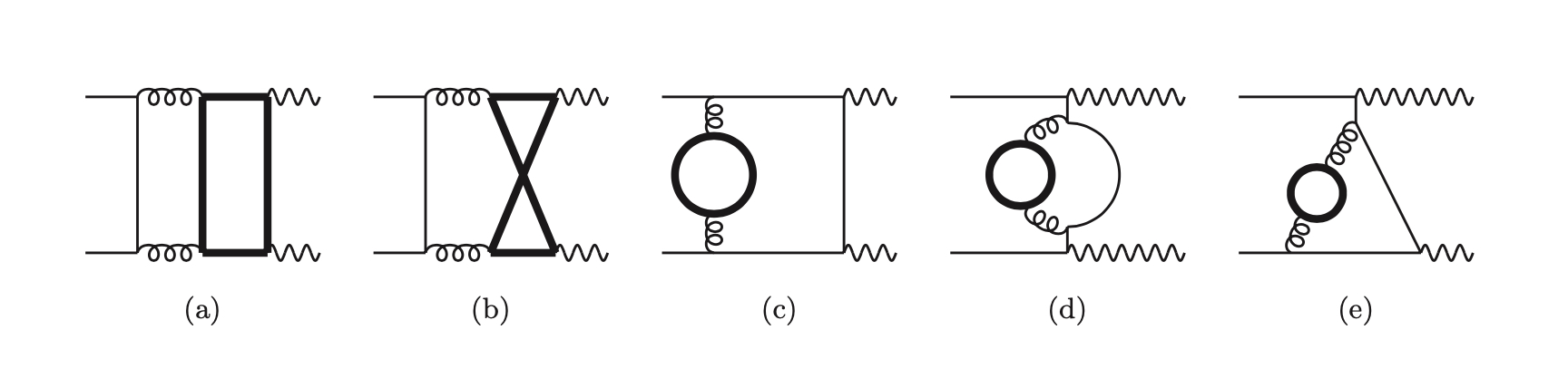
Figure 1: Representative set of two-loop diagrams with internal heavy-quark loops, which contribute at NNLO QCD corrections to diphoton production in the quark annihilation channel. Thin black lines represents light quarks, thick black lines heavy quarks, curly lines gluons and curby lines photons.

where the external particles are on-shell, i.e. $p_{i}^{2}=0$, and we indicate with $m_{t}^{2}$ the heavy-quark squared mass. In order to obtain the scattering amplitude, we generated the relevant Feynman diagrams using the $\tt{FeynArts}$ package Hahn:2000kx . We found a total number of 14 diagrams contributing to the amplitude, the representative ones are shown in fig. 1. We write the scattering amplitude in terms of form factors, which are decomposed into a basis of 72 MIs exploiting IBPs reduction Chetyrkin:1979bj ; Chetyrkin:1981qh ; Laporta:2001dd ; Lee:2012cn ; Lee:2013mka ; Smirnov:2008iw ; Smirnov:2014hma ; Studerus:2009ye ; vonManteuffel:2012np ; Peraro:2019svx ; Maierhofer:2017gsa , as implemented in the software $\tt{Kira}$ Maierhofer:2017gsa .

The MIs contributing to this process can be described by three different scalar integral topologies (modulo exchange of the two final photons). Specifically, the MIs for the Feynman diagrams (a) and (b) in fig. 1 are associated to the integral families PLA and NPL, respectively, as defined in section 3. Similarly, the MIs for the diagrams (c), (d) and (e) can be grouped into one scalar integral family, PLB, also defined in section 3. The MIs of the families PLA and PLB were already known in the literature Becchetti:2017abb . Regarding the non-planar topology NPL, while most of the MIs have already been studied Becchetti:2017abb ; Bonciani:2007eh ; Bonciani:2008ep ; Aglietti:2006tp ; Anastasiou:2006hc ; vonManteuffel:2017hms ; Bonciani:2018uvv , the double-box top-sector have not been considered in the literature yet, and therefore its computation represents an original result by itself.

For this project, we performed an independent calculation of all the MIs by means of the differential equations method Kotikov:1990kg ; Kotikov:1991pm ; Bern:1993kr ; Remiddi:1997ny ; Gehrmann:1999as ; Argeri:2007up ; Henn:2013pwa ; Henn:2014qga . In particular we solved the system of differential equations semi-analytically exploiting the generalised power series expansion technique, as described in Moriello:2019yhu and implemented in the software $\tt{DiffExp}$ Hidding:2020ytt .

The two-loop amplitudes computed in this paper constitute a necessary ingredient of the recently presented full massive NNLO QCD corrections to diphoton production at hadron colliders Becchetti:ta . We anticipate here, that our two-loop form factors, taking into account the full dependence on the top quark mass, are finite (free of IR divergences after UV renormalization). Therefore, they can be included directly (without the use of any IR regularization prescription) in any numerical implementation of the NNLO cross section. In the following paragraph we will illustrate the precedent statement with a specific example based on the $q_{T}$-subtraction method Catani:2007vq ; Catani:2013tia (which can easily be extended to any other subtraction method).

To this end, we consider the following scattering process,

$$h_{1}+h_{2}\rightarrow\gamma\gamma$$ (3)

where $h_{1}$ and $h_{2}$ are the colliding hadrons. At the NNLO, the cross-section for this process can be computed using the $q_{T}$-subtraction method Bozzi:2005wk ; Catani:2007vq ; Catani:2013tia as follows

$$d\sigma^{\gamma\gamma}_{\rm NNLO}=\mathcal{H}^{\gamma\gamma}_{\rm NNLO}\otimes d\sigma^{\gamma\gamma}_{\rm LO}+\left[d\sigma^{\gamma\gamma+{\rm jets}}_{\rm NLO}-d\sigma^{CT}_{\rm NLO}\right].$$ (4)

The terms inside the square brackets $d\sigma^{\gamma\gamma+jets}_{\rm NLO}$ and $d\sigma^{CT}_{\rm NLO}$ represent the cross section for diphoton plus jet production at NLO DelDuca:2003uz and the corresponding counterterm, needed to cancel the associated singularities in the small-$q_{T}$ limit. The coefficient function $\mathcal{H}^{\gamma\gamma}_{\rm NNLO}$ (defined in Bozzi:2005wk ) is the so-called hard-virtual function and it includes the one-loop and two-loop corrections to the Born subprocess. This object admits a perturbative expansion in terms of the strong coupling $\alpha_{S}$:

$$\mathcal{H}^{\gamma\gamma}=1+\frac{\alpha_{S}}{\pi}\mathcal{H}^{\gamma\gamma}_{\rm NLO}+\left(\frac{\alpha_{S}}{\pi}\right)^{2}\mathcal{H}^{\gamma\gamma}_{\rm NNLO}+\cdots\,.$$ (5)

In our particular case (diphoton production) the one-loop contribution to eq. (5) was calculated in Balazs:1997hv , while the massless two-loop contribution was first calculated in Anastasiou:2002zn and later in Caola:2022dfa . The explicit expressions of the hard virtual factor (computed with the previous massless one- and two-loop amplitudes) in the hard resummation scheme are given in Appendix A of ref. Catani:2013tia . The inclusion of the new two-loop massive form factors proceeds by simple addition to that of the massless case Anastasiou:2002zn . After regularising the IR divergences (e.g. in the in the hard resummation scheme) Catani:2013tia present in the massless two-loop amplitude Anastasiou:2002zn , our massive two-loop contribution can be added directly to the massless finite remainder.

After generating all the relevant Feynman diagrams for the process, the amplitude $\mathcal{A}_{q\bar{q},\gamma\gamma}$ has been decomposed in terms of form factors Peraro:2020sfm , and the UV singularities have been regularised in dimensional regularisation. The expression obtained has been used to compute the NNLO corrections to the hard function $\mathcal{H}^{\gamma\gamma}$ coming from two-loop diagrams which involve a massive top quark loop. Specifically, from the knowledge of the finite remainder $\mathcal{A}^{(\text{fin})}_{q\bar{q},\gamma\gamma}$ of the amplitude, we can obtain the hard function from the all-orders relation Catani:2013tia :

$$\mathcal{H}^{\gamma\gamma}=\frac{|\mathcal{A}^{(\text{fin})}_{q\bar{q},\gamma\gamma}|^{2}}{|\mathcal{A}_{q\bar{q},\gamma\gamma}^{(0)}|^{2}},$$ (6)

where $\mathcal{A}_{q\bar{q},\gamma\gamma}^{(0)}$ is the Born-level amplitude for this process:

$$|\mathcal{A}_{q\bar{q},\gamma\gamma}^{(0)}|^{2}=128\,\pi^{2}\,\alpha_{em}^{2}\,Q_{q}^{4}\,N_{c}\left(\frac{t}{u}+\frac{u}{t}\right),$$ (7)

with $\alpha_{em}$, the QED coupling, $Q_{q}$ is the electric charge of the incoming quarks and $N_{c}$ is the number of colours. We also performed a sum over initial and final polarisations and initial colours.

This massive hard-virtual coefficient represents the last missing ingredient necessary to perform a NNLO phenomenological study, for diphoton production at the LHC, which takes into account the complete dependence on the top quark mass Becchetti:ta .

2.1 Form factors

The bare scattering amplitude can be written as

$$\mathcal{A}_{q\bar{q},\gamma\gamma}=\alpha_{em}\,\delta_{ij}\,\epsilon^{\ast\mu}_{\lambda_{3}}(p_{3})\epsilon^{\ast\nu}_{\lambda_{4}}(p_{4})\overline{v}_{s_{2}}(p_{2})\mathcal{A}_{\mu\nu}(s,t,u,m_{t}^{2})u_{s_{1}}(p_{1}),$$ (8)

where $\delta_{ij}$ is the Kronecker delta function with $i$ and $j$ the color indices of the incoming $q\bar{q}$ pair, $\epsilon^{\ast\mu}_{\lambda_{3}}(p_{3})$ and $\epsilon^{\ast\nu}_{\lambda_{4}}(p_{4})$ are external photon polarisation vectors and $\overline{v}_{s_{2}}(p_{2})$, $u_{s_{1}}(p_{1})$ the quark spinors.

The amplitude (8) can be further decomposed in terms of a set of four independent tensors Peraro:2020sfm which are built using external momenta and polarisation vectors:

$$\mathcal{A}_{q\bar{q},\gamma\gamma}=\sum_{k=1}^{4}\mathcal{F}_{k}\,T_{k},$$ (9)

where the $T_{k}$ are chosen as:

$$\begin{split}T_{1}&=\overline{v}_{s_{2}}(p_{2})\not{\epsilon}^{\ast}_{\lambda_{3}}(p_{3})u_{s_{1}}(p_{1})\epsilon^{\ast}_{\lambda_{4}}(p_{4})\cdot p_{2},\\ T_{2}&=\overline{v}_{s_{2}}(p_{2})\not{\epsilon}^{\ast}_{\lambda_{4}}(p_{4})u_{s_{1}}(p_{1})\epsilon^{\ast}_{\lambda_{3}}(p_{3})\cdot p_{1},\\ T_{3}&=\overline{v}_{s_{2}}(p_{2})\not{p}_{3}u_{s_{1}}(p_{1})\epsilon^{\ast}_{\lambda_{3}}(p_{3})\cdot p_{1}\epsilon^{\ast}_{\lambda_{4}}(p_{4})\cdot p_{2},\\ T_{4}&=\overline{v}_{s_{2}}(p_{2})\not{p}_{3}u_{s_{1}}(p_{1})\epsilon^{\ast}_{\lambda_{3}}(p_{3})\cdot\epsilon^{\ast}_{\lambda_{4}}(p_{4}).\end{split}$$ (10)

The decomposition (9) has been achieved also by enforcing the physical conditions $\epsilon_{\lambda_{i}}\cdot p_{i}=0$ for the polarisation vectors, and by choosing as reference vectors for the external photons the condition $\epsilon_{\lambda_{3}}\cdot p_{2}=\epsilon_{\lambda_{4}}\cdot p_{1}=0$, which implies for the photons the polarization sums:

$$\sum_{\lambda_{3}}\epsilon_{\lambda_{3}}^{\mu}\epsilon_{\lambda_{3}}^{*\nu}=g^{\mu\nu}-\frac{p_{2}^{\mu}p_{3}^{\nu}+p_{3}^{\mu}p_{2}^{\nu}}{p_{2}\cdot p_{3}},\hskip 28.45274pt\sum_{\lambda_{4}}\epsilon_{\lambda_{4}}^{\mu}\epsilon_{\lambda_{4}}^{*\nu}=g^{\mu\nu}-\frac{p_{1}^{\mu}p_{4}^{\nu}+p_{4}^{\mu}p_{1}^{\nu}}{p_{1}\cdot p_{4}},$$ (11)

where $g^{\mu\nu}=\operatorname{diag}(1,1,1,1)$. The coefficients of $T_{k}$ are the so-called scalar form factors, $\mathcal{F}_{k}$. These objects are functions of the kinematic invariants of the process, and of the space-time dimension $D$, and they can be written in terms of scalar Feynman integrals. Their expression can be obtained by applying a set of projectors, $\left\{\mathcal{P}_{k}\right\}$, $k=1,2,3,4$, to the amplitude $\mathcal{A}_{q\bar{q},\gamma\gamma}$:

$$\mathcal{F}_{k}=\operatorname{tr}\left\{\sum_{s_{1},s_{2},\lambda_{3},\lambda_{4}}\mathcal{P}_{k}\,\mathcal{A}_{q\bar{q},\gamma\gamma}\right\},$$ (12)

where

$$\mathcal{P}_{1} =\frac{1}{(D-3)t}\left[\frac{u}{2s^{2}}T_{1}^{{\dagger}}-\frac{u}{2s^{2}t}T_{3}^{{\dagger}}\right],$$

$$\mathcal{P}_{2} =\frac{1}{(D-3)t}\left[\frac{u}{2s^{2}t}T_{3}^{{\dagger}}+\frac{u}{2s^{2}}T_{2}^{{\dagger}}\right],$$

$$\mathcal{P}_{3} =\frac{1}{(D-3)t}\left[\frac{\left(Du^{2}-4st\right)}{2s^{2}ut^{2}}T_{3}^{{\dagger}}-\frac{u}{2s^{2}t}T_{1}^{{\dagger}}+\frac{u}{2s^{2}t}T_{2}^{{\dagger}}+\frac{(t-s)}{2sut}T_{4}^{{\dagger}}\right],$$

$$\mathcal{P}_{4} =\frac{1}{(D-3)t}\left[\frac{(t-s)}{2sut}T_{3}^{{\dagger}}+\frac{1}{2u}T_{4}^{{\dagger}}\right].$$ (13)

The form factors $\mathcal{F}_{k}$ admit the following perturbative expansion:

$$\mathcal{F}_{k}=\mathcal{F}_{k}^{(0)}+\left(\frac{\alpha_{S}}{\pi}\right)\mathcal{F}_{k}^{(1)}+\left(\frac{\alpha_{S}}{\pi}\right)^{2}\mathcal{F}_{k}^{(2)}+\cdots\,,$$ (14)

where $\alpha_{S}$ is the strong coupling constant. At leading order we have:

$$\mathcal{F}_{1}^{(0)} =-4\pi\alpha_{em}\delta_{ij}Q_{q}^{2}\,\frac{1}{t}\,,$$

$$\mathcal{F}_{2}^{(0)} =4\pi\alpha_{em}\delta_{ij}Q_{q}^{2}\,\frac{1}{t}\,,$$

$$\mathcal{F}_{3}^{(0)} =4\pi\alpha_{em}\delta_{ij}Q_{q}^{2}\,\frac{2}{tu}\,,$$

$$\mathcal{F}_{4}^{(0)} =-4\pi\alpha_{em}\delta_{ij}Q_{q}^{2}\,\frac{(t-u)}{tu}\,.$$ (15)

The massive corrections, we are interested in, appear starting from the two-loop order. Therefore, they affect only the term $\mathcal{F}_{k}^{(2)}$. For the rest of this paper we will focus just on this contribution, which we will refer to as $\mathcal{F}_{k,\texttt{top}}^{(2)}$. We generated all the relevant Feynman diagrams for this contribution using FeynArts Hahn:2000kx , and we found 14 different two-loop Feynman diagrams, which can be grouped into five different categories, as depicted in fig. 1. We used FORM Kuipers:2012rf ; Ruijl:2017dtg to apply the projectors to the Feynman diagrams and perform the Dirac algebra. The form factors, then, were expressed as a linear combinations of 72 MIs, $\left\{\mathcal{J}_{i}\right\}$, which are defined in Appendix A.

We find the following expression for the form factors $\mathcal{F}_{k,\texttt{top}}^{(2)}$:

$$\mathcal{F}_{k,\texttt{top}}^{(2)}=4\pi\alpha_{em}\delta_{ij}\,C_{F}\left[Q_{q}^{2}\mathcal{F}_{k,\texttt{top};0}^{(2)}+Q_{t}^{2}\mathcal{F}_{k,\texttt{top};2}^{(2)}\right]\,,$$ (16)

where $C_{F}=\frac{N_{c}^{2}-1}{2N_{c}}$ is the Casimir of the fundamental representation of $SU(N_{c})$ and $Q_{t}$ is the electric charge of the top quark running in the loop. The two contributions $\mathcal{F}_{k,\texttt{top};0}^{(2)}$ and $\mathcal{F}_{k,\texttt{top};2}^{(2)}$ are indeed related to different powers of the top electric charge $Q_{t}$. The first contribution $\mathcal{F}_{k,\texttt{top};0}^{(2)}$ is associated to the diagrams (c), (d) and (e) in fig. 1 in which the top quark does not couple to the external photons, while the second contribution $\mathcal{F}_{k,\texttt{top};2}^{(2)}$ comes from the diagrams (a) and (b) where the top quark actually couples with the photon.

We perform our computations in the context of dimensional regularisation. As a consequence, potential ultraviolet (UV) and infrared (IR) singularities can appear in the form factors as poles in the dimensional regulator $\epsilon=(4-D)/2$. However, since the diagrams with a top loop start contributing to the $q\bar{q}$ channel at the two-loop order, $\mathcal{F}_{k,\texttt{top}}^{(2)}$ does not have IR singularities and therefore all the $\epsilon$ poles are of UV origin. Furthermore, $\mathcal{F}_{k,\texttt{top};2}^{(2)}$ is also free of UV divergences and then the UV poles come only from the contribution $\mathcal{F}_{k,\texttt{top};0}^{(2)}$.

2.2 UV Renormalisation

We renormalise the bare form factors in a mixed scheme. The external quark fields are renormalised on shell; the strong coupling constant is renormalised in a scheme in which the light-quark contribution is treated in $\overline{\mbox{MS}}$, while the heavy-quark contribution is renormalised at zero momentum. No renormalisation is needed for the top quark mass $m_{t}^{2}$ at this order in perturbation theory and the same occurs for the external photon field.

We have, then

$$\mathcal{F}_{k}^{R}=Z_{q}\,\mathcal{F}_{k}\left(\alpha_{S}^{B}\to Z_{\alpha_{S}}\alpha_{S}\right)\,,$$ (17)

where the superscript “R” stands for “renormalised”. The renormalisation factors $Z_{q}$ and $Z_{\alpha_{S}}$ admit a perturbative expansion in the strong coupling constant Barnreuther:2013qvf ; Broadhurst:1993mw ; Melnikov:2000qh ; Mitov:2006xs :

$$Z_{q} =1+\left(\frac{\alpha_{S}}{\pi}\right)\delta Z_{q}^{(1)}+\left(\frac{\alpha_{S}}{\pi}\right)^{2}\delta Z_{q}^{(2)}+\mathcal{O}(\alpha_{S}^{4})\,,$$

$$Z_{\alpha_{S}} =1+\left(\frac{\alpha_{S}}{\pi}\right)\delta Z_{\alpha}^{(1)}+\mathcal{O}(\alpha_{S}^{2})\,.$$ (18)

In our renormalisation scheme, we have

$$\delta Z_{q}^{(1)} =0\,,$$

$$\delta Z_{q}^{(2)} =\pi^{-2\epsilon}\Gamma^{2}(1+\epsilon)\,\left(\frac{\mu^{2}}{m_{t}^{2}}\right)^{2\epsilon}\,C_{F}N_{h}T_{F}\,\left(\frac{1}{16\epsilon}-\frac{5}{96}\right)\,,$$

$$\delta Z_{\alpha}^{(1)} =\delta Z_{\alpha,N_{l},\overline{\mathrm{MS}}}^{(1)}+\delta Z_{\alpha,N_{h},\mathrm{OS}}^{(1)}\,,$$ (19)

where

$$\delta Z_{\alpha,N_{l},\overline{\mathrm{MS}}}^{(1)} =-\pi^{-\epsilon}e^{-\gamma\epsilon}\frac{1}{2\epsilon}\left(\frac{11}{6}C_{A}-\frac{1}{3}N_{l}\right)\,,$$

$$\delta Z_{\alpha,N_{h},\mathrm{OS}}^{(1)} =\pi^{-\epsilon}\Gamma(1+\epsilon)\,\left(\frac{\mu^{2}}{m_{t}^{2}}\right)^{\epsilon}\,\frac{N_{h}}{6\epsilon}\,,$$ (20)

$\mu$ is the renormalisation scale, $N_{l}$ is the number of light flavours, in this case $N_{l}=5$, $N_{h}$ is the number of heavy quarks, in this case $N_{h}=1$, the quantity $C_{A}=N_{c}$ is the Casimir of the adjoint representation of $SU(N_{c})$, and $T_{F}=\frac{1}{2}$.

Therefore, the renormalised form factors $\mathcal{F}_{k,\texttt{top}}^{(2)\,R}$ are determined by the following formula:

$$\mathcal{F}_{k,\texttt{top}}^{(2)\,R}=\mathcal{F}_{k,\texttt{top}}^{(2)}+\delta Z_{q}^{(2)}\,\mathcal{F}_{k}^{(0)}+\delta Z_{\alpha,N_{h},\mathrm{OS}}^{(1)}\,\mathcal{F}_{k}^{(1)}\,.$$ (21)

3 Master Integrals Computation

In this section we discuss the details of the MIs computation. Specifically, we define the three scalar integral topologies which describe all the MIs that appear in the amplitude (modulo exchange of final photons). The MIs are computed through the differential equations method. The system of differential equations associated to the MIs is solved semi-analytically employing the generalised power series expansion technique, as described in Moriello:2019yhu and implemented in the software $\tt{DiffExp}$ Hidding:2020ytt . Finally, we show that some of the MIs that appear in the computation admit an analytic solution in terms of elliptic functions.

The system of differential equations for the planar families, PLA and PLB, is in canonical form, while for the non-planar family, NPL, we have canonical differential equations just for the sectors whose analytic solution could be given in terms of MPLs. We notice that the bases of MIs in which we solve the differential equations, which we will refer in the following as $\vec{f}$ for the planar families and $\vec{g}$ for the non-planar one, and the one in which we write the form factors are different. We choose this approach in order to avoid square roots of the kinematic invariants in the expressions of the form factors. In the ancillary material attached to this paper, we furnish the rotation matrices from the bases $\vec{f}$ and $\vec{g}$ to the basis $\left\{\mathcal{J}_{i}\right\}$ defined in Appendix A.

3.1 General Setup

The three integral families which describe the relevant MIs for this process are defined as follows:

$$\mathcal{I}_{\texttt{topo}}(n_{1},...,n_{9})=\int\frac{\mathcal{D}k_{1}\mathcal{D}k_{2}}{D_{1}^{n_{1}}D_{2}^{n_{2}}D_{3}^{n_{3}}D_{4}^{n_{4}}D_{5}^{n_{5}}D_{6}^{n_{6}}D_{7}^{n_{7}}D_{8}^{n_{8}}D_{9}^{n_{9}}},$$ (22)

where topo $\in\left\{\text{PLA},\text{PLB},\text{NPL}\right\}$ labels the families and the scalar products $D_{1},...,D_{9}$ are given in table 1. The indices $n_{1},\cdots,n_{7}$ are non-negative while the indices $n_{8}$ and $n_{9}$ are non-positive.

The computation is done in dimensional regularization with $D=4-2\epsilon$ dimensions, and our convention for the integration measure is

$$\mathcal{D}k=\frac{\operatorname{d}^{D}k}{i\pi^{2-\epsilon}\Gamma(1+\epsilon)}\left(\frac{\mu^{2}}{m_{t}^{2}}\right)^{-\epsilon}\,,$$ (23)

where $\mu$ is the dimensional regularization scale.

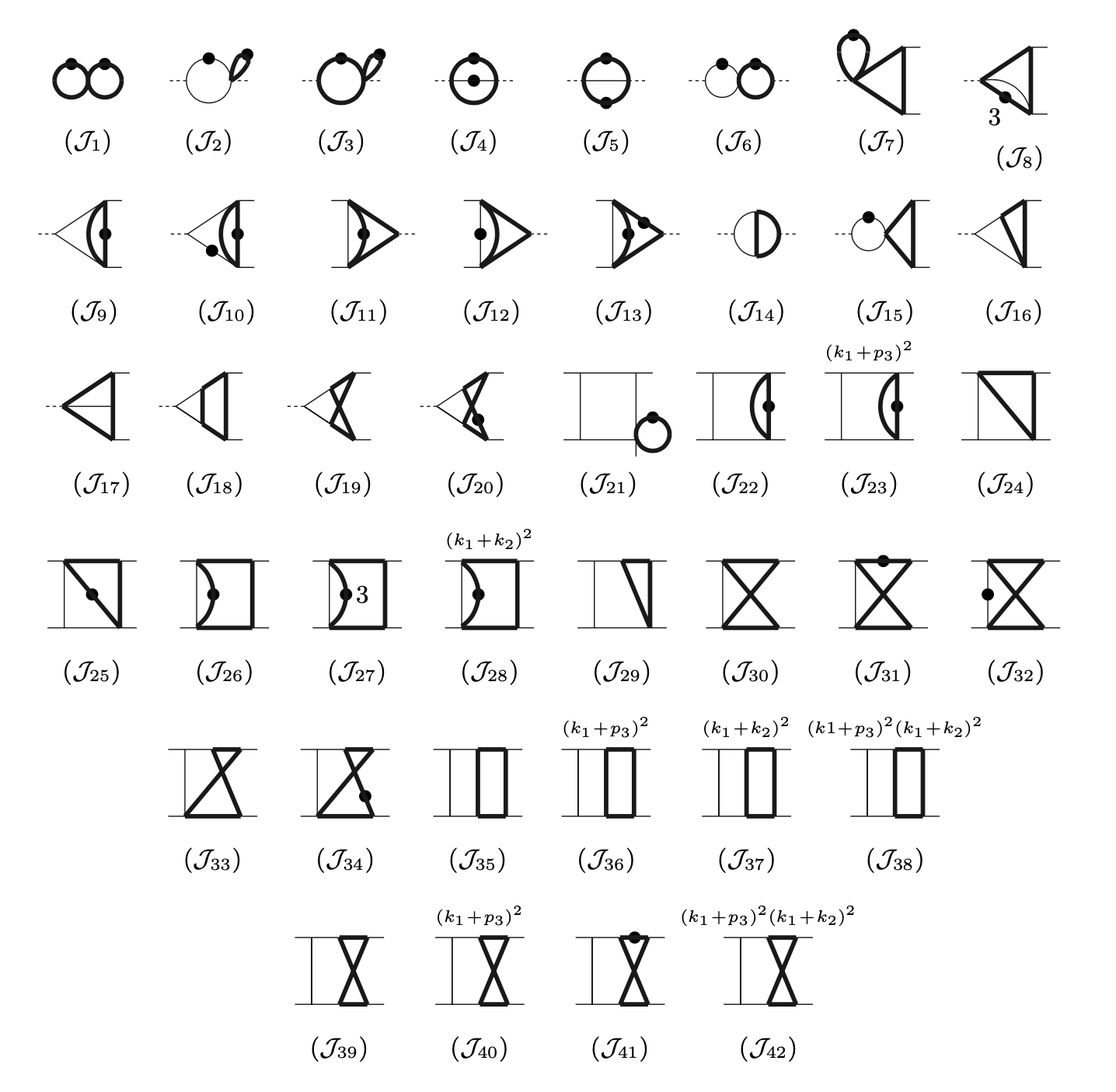
Figure 2: Basis of Master Integrals for the topologies PLA, PLB and NPL. In the figure, the MIs defined with a permutation of the external momenta are not displayed.

With the definitions given in table 1, all the scalar Feynman integrals appearing in the amplitude can be mapped to one of the three integral families, or families obtained by permutation of the external momenta. The MIs appearing in the form factors are listed in appendix A and shown in fig. 2.

Denominator	Integral family PLA	Integral family PLB	Integral family NPL
$D_{1}$	$k_{1}^{2}$	$k_{1}^{2}$	$k_{1}^{2}$
$D_{2}$	$(k_{1}-p_{1})^{2}$	$(k_{1}-p_{1})^{2}$	$(k_{1}-p_{1})^{2}$
$D_{3}$	$(k_{1}+p_{2})^{2}$	$(k_{1}+p_{2})^{2}$	$(k_{1}+p_{2})^{2}$
$D_{4}$	$k_{2}^{2}+m_{t}^{2}$	$k_{2}^{2}+m_{t}^{2}$	$k_{2}^{2}+m_{t}^{2}$
$D_{5}$	$(k_{1}+k_{2}-p_{1})^{2}+m_{t}^{2}$	$(k_{2}-k_{1})^{2}+m_{t}^{2}$	$(k_{1}+k_{2}-p_{1})^{2}+m_{t}^{2}$
$D_{6}$	$(k_{1}+k_{2}+p_{2})^{2}+m_{t}^{2}$	$(k_{1}-p_{1}+p_{3})^{2}$	$(k_{2}-p_{1}-p_{2}+p_{3})^{2}+m_{t}^{2}$
$D_{7}$	$(k_{1}+k_{2}-p_{1}+p_{3})^{2}+m_{t}^{2}$	$(k_{2}+p_{1})^{2}$	$(k_{1}+k_{2}-p_{1}+p_{3})^{2}+m_{t}^{2}$
$D_{8}$	$(k_{1}+p_{3})^{2}$	$(k_{2}+p_{2})^{2}$	$(k_{1}+p_{3})^{2}$
$D_{9}$	$(k_{1}+k_{2})^{2}$	$(k_{2}+p_{3})^{2}$	$(k_{1}+k_{2})^{2}$

Table 1: Routing definition for the three scalar integrals families PLA, PLB and NPL.

3.2 Planar Families PLA and PLB

The scalar integrals family PLA is described by a set of 32 master integrals $\vec{f}(\vec{x},\epsilon)$, where

$$\vec{x}=\left\{y,z\right\},\;\;\;y=\frac{s}{m_{t}^{2}},\;z=\frac{t}{m_{t}^{2}}$$ (24)

is the vector of the kinematic invariants with respect to which we derived the differential equations. The system of differential equations for these integrals has been derived in canonical logarithmic form Henn:2013pwa in ref. Becchetti:2017abb :

$$d\,\vec{f}(\vec{x},\epsilon)=\epsilon\,d\,A(\vec{x})\vec{f}(\vec{x},\epsilon),$$ (25)

where $d$ is the total differential with respect to the kinematic invariants, and the matrix $A(\vec{x})$ is written as linear combinations of logarithms:

$$A(\vec{x})=\sum c_{i}\log(w_{i}(\vec{x})).$$ (26)

The $c_{i}$ represent matrices of rational numbers, while $\mathbf{W}_{PLA}=\left\{w_{i}(\vec{x})\right\}$ is the alphabet of the solution and it is made by algebraic functions of the kinematic invariants. Specifically, the alphabet is made by the following set of 21 letters:

$$\mathbf{W}_{PLA}=\biggl{\{} r_{1},r_{2},r_{3},r_{4},\frac{r_{4}-r_{5}}{r_{4}+r_{5}},y,\frac{r_{1}-y}{r_{1}+y},r_{4}-r_{2}y,\frac{r_{3}+y}{r_{3}-y},\frac{-r_{1}z+r_{1}+r_{5}}{-r_{1}z+r_{1}-r_{5}},\frac{r_{5}-yz+y}{y-yz},\frac{r_{1}z-r_{4}}{r_{1}z+r_{4}},$$

$$\frac{r_{1}z-r_{5}}{r_{1}z+r_{5}},1-z,z,y+z,\frac{r_{2}-z}{r_{2}+z},-\frac{r_{5}-yz+y+2z}{r_{5}-yz+y-2z^{2}},\frac{r_{4}z+r_{4}-r_{5}z}{r_{4}z+r_{4}+r_{5}z},-\frac{-r_{2}+r_{3}+y+z}{r_{2}+r_{3}+y+z},$$

$$\frac{-r_{2}y(z-4)+r_{2}z(r_{2}-z+4)+r_{4}(z-4)}{r_{2}y(z-4)+r_{2}z(r_{2}+z-4)-r_{4}(z-4)}\biggr{\}},$$ (27)

where $r_{1},\cdots,r_{5}$ are a set of square roots of the kinematic invariants:

$$\begin{split}r_{1}&=\sqrt{(y-4)y},\hskip 14.22636ptr_{2}=\sqrt{(z-4)z},\hskip 14.22636ptr_{3}=\sqrt{y(y+4)},\hskip 14.22636ptr_{4}=\sqrt{yz(y(z-4)-4z)},\\ r_{5}&=\sqrt{y\left(y(z-1)^{2}-4z^{2}\right)}.\end{split}$$ (28)

The knowledge of the logarithmic canonical form of the differential equations (25), together with the alphabet structure (3.2) would allow us, in principle, to obtain a fully analytic representation for the system of the MIs. However, the presence of the set of square roots given in Eq. (28) makes the achievement of such analytic expression non trivial. Indeed, these square roots are not simultaneously rationalizable. As a consequence, in order to obtain a fully analytic representation of the solution one would have to exploit symbol level techniques Goncharov:2010jf ; Duhr:2011zq . For the purpose of this project, we found that the semi-analytic evaluation, which we achieved exploiting a generalised power series expansion method, was sufficient to perform phenomenological studies.

The boundary conditions for the system are provided in the origin of kinematic variables $y=z=0$, where all the MIs vanish except for the two masters $f_{1}$ and $f_{2}$, for which we use the following analytical expressions:

$$f_{1} =\epsilon^{2}\,\mathcal{J}_{1}=1,$$

$$f_{2} (y)=-y\,\epsilon^{2}\,\mathcal{J}_{2}(y)=-\left(-y\right)^{-\epsilon}\frac{\Gamma(1-\epsilon)^{2}}{\Gamma(1-2\epsilon)},$$ (29)

where $\mathcal{J}_{1}$ and $\mathcal{J}_{2}$ are the pre-canonical masters shown in fig. 2 and defined in Appendix A.

Regarding the second planar family, PLB, we observe that we do not need to set up a system of differential equations for it. Indeed, every master integral of this family, except $\mathcal{J}_{21}$, is equal to one of the MIs of the two other families (modulus permutations). For $\mathcal{J}_{21}$, by integrating analytically its differential equation, we obtain the following analytical expression:

$$\mathcal{J}_{21}(y,z)= \frac{1}{y\,z}\left[\frac{4}{\epsilon^{3}}\,-\,\frac{2(\log(-y)+\log(-z))}{\epsilon^{2}}\,-\,\frac{5\pi^{2}-6\log(-y)\log(-z)}{3\epsilon}\,+\,\right.$$

$$+2\text{Li}_{3}\left(-\frac{z}{y}\right)-2\log(-z)\text{Li}_{2}\left(-\frac{z}{y}\right)+2\log(-y)\text{Li}_{2}\left(-\frac{z}{y}\right)$$

$$-\log(-y)\log^{2}(-z)+\log(y)\log^{2}(-z)-\log^{2}(-z)\log(y+z)$$ (30)

$$-\log^{2}(-y)\log(y+z)-2\log(-y)\log(y)\log(-z)$$

$$+2\log(-y)\log(-z)\log(y+z)-\pi^{2}\log(y+z)$$

$$+\log^{2}(-y)\log(y)+\frac{\pi^{2}}{3}\log(-y)+\pi^{2}\log(y)$$

$$\left.\quad+\frac{1}{3}\log^{3}(-z)+\frac{4}{3}\pi^{2}\log(-z)-10\zeta(3)\right]\;+\;\mathcal{O}(\epsilon).$$

This formula was cross checked analytically with Henn_2015 and numerically with AMFlow Liu_2023 .

3.3 Non-Planar Family NPL

The non-planar scalar integrals family, NPL, is more complicated to study with respect to the two planar families. The total number of MIs $\vec{g}$ associated to this topology is 36. The system of differential equations can be divided in two different subsets:

• (I) Canonical logarithmic: the subset of MIs whose differential equations is in canonical logarithmic form;

• (II) Elliptic sectors: this subset contains MIs whose analytic solution involve elliptic functions and it is not written in $\epsilon$-factorized form.

The system of differential equations for the subset (I) has been put in canonical logarithmic form. The alphabet $\mathbf{W}_{NPL}$ for this subset is described by the following 30 letters:

$$\mathbf{W}_{NPL}=\biggl{\{} q_{1},q_{3},q_{4},q_{5},q_{6},-\frac{q_{4}-2q_{8}}{q_{4}+2q_{8}},\frac{q_{5}-2q_{8}}{q_{5}+2q_{8}},-\frac{q_{9}-2}{q_{9}+2},q_{9},-\frac{q_{7}y+q_{5}}{q_{5}-q_{7}y},y,-\frac{q_{1}+y}{y-q_{1}},$$

$$q_{4}-q_{2}y,-\frac{q_{3}+y}{y-q_{3}},\frac{q_{1}z-q_{4}}{q_{1}z+q_{4}},-\frac{q_{6}-q_{7}z}{q_{7}z+q_{6}},z,y+z,y+z+4,-\frac{q_{2}+z}{z-q_{2}},\frac{q_{1}y+q_{1}z+q_{5}}{q_{1}y+q_{1}z-q_{5}},$$

$$\frac{q_{2}y+q_{2}z+q_{6}}{q_{2}y+q_{2}z-q_{6}},\frac{-q_{5}+y^{2}+yz}{q_{5}+y^{2}+yz},\frac{q_{3}y-q_{7}y+q_{3}z}{q_{3}y+q_{7}y+q_{3}z},\frac{-q_{6}+yz+z^{2}}{q_{6}+yz+z^{2}},\frac{q_{6}+yz+z^{2}}{-q_{6}+yz+z^{2}},$$

$$-\frac{q_{7}+y+z}{-q_{7}+y+z},-\frac{q_{2}+q_{3}+y+z}{-q_{2}+q_{3}+y+z},-\frac{q_{8}yz-4q_{8}y+q_{6}q_{9}y+q_{8}z^{2}-4q_{8}z-2q_{8}q_{9}z}{q_{8}yz-4q_{8}y+q_{6}q_{9}y+q_{8}z^{2}-4q_{8}z+2q_{8}q_{9}z},$$

$$\frac{-q_{2}y-q_{2}z+q_{4}+z^{2}}{q_{2}y+q_{2}z-q_{4}+z^{2}}\biggr{\}}$$ (31)

where $q_{1},\cdots,q_{9}$ are a set of square roots of the kinematic invariants:

$$\begin{split}q_{1}&=\sqrt{y(y-4)},\hskip 14.22636ptq_{2}=\sqrt{z(z-4)},\hskip 14.22636ptq_{3}=\sqrt{y(y+4)},\hskip 14.22636ptq_{4}=\sqrt{yz(y(z-4)-4z)},\\ q_{5}&=\sqrt{y(y+z)(-4z+y(y+z))},\hskip 14.22636ptq_{6}=\sqrt{z(y+z)\left(y(z-4)+z^{2}\right)},\hskip 14.22636ptq_{7}=\sqrt{(y+z)(y+z+4)},\\ q_{8}&=\sqrt{-yz(y+z)},\hskip 14.22636ptq_{9}=\sqrt{4-z}.\end{split}$$ (32)

The subset (II), which is associated to MIs whose analytic structure involve elliptic functions, contains two sectors (see fig. 3). The first one is a non-planar triangle with a massive loop vonManteuffel:2017hms , shown in fig. 3 (a).

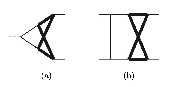
Figure 3: Diagrams representing the two elliptic sectors in the non planar topology NPL. Thin lines represent massless particles, while thick lines massive particles.

This sector has 2 MIs, which admit a representation in terms of elliptic multiple polylogarithms (eMPLs) Broedel:2019hyg .

We choose for them the same normalization as in vonManteuffel:2017hms :

$$g_{31}(y)=y^{2}\epsilon^{4}\mathcal{J}_{19}\,,\hskip 14.22636ptg_{32}(y)=-\frac{y^{2}\epsilon^{4}\left(16+y\right)}{2(1+2\epsilon)}\mathcal{J}_{20}\,.$$ (33)

The second sector whose analytic structure is characterised by the presence of elliptic functions is the top sectors of the topology NPL, i.e. the double-box integral, shown in fig. 3 (b), which contains 4 MIs: $g_{33},g_{34},g_{35}$ and $g_{36}$. We choose, as basis for this sector, the following scalar integrals:

$$\begin{split}g_{33}(y,z)&=-y^{3}\epsilon^{4}\mathcal{J}_{39},\hskip 14.22636ptg_{34}(y,z)=y^{2}\epsilon^{4}\mathcal{J}_{40}\,,\\ g_{35}(y,z)&=y^{4}\epsilon^{4}\mathcal{J}_{41}\,,\hskip 14.22636ptg_{36}(y,z)=-y\epsilon^{4}\mathcal{J}_{42}\,.\end{split}$$ (34)

With this choice of normalization, initial conditions in the origin $y=z=0$ are:

$$g_{1}=f_{1},\hskip 14.22636ptg_{2}(y)=f_{2}(y),\hskip 14.22636ptg_{i}(y=0,z=0)=0,\hskip 14.22636pti=3,\dots,36$$ (35)

where $f_{1}$ and $f_{2}$ are given in Eq. (29).

The non-polylogarithmic structure of this sector is two-fold. First, the differential equations for the MIs $g_{33}$, $g_{34}$, $g_{35}$ and $g_{36}$ contain the triangle integrals $g_{31}$ and $g_{32}$ in the non-homogeneous part of the system. As a consequence the analytic solution of the differential equations requires the integration over kernels that contains eMPLs. Moreover, also the homogeneous part of the differential equations itself contains elliptic functions. This statement can be verified by studying the maximal cut of the double-box integral Henn:2014qga :

$$\mathcal{I}_{db}=\mathcal{J}_{39}\,.$$ (36)

In order to perform such computation it is convenient to follow the loop-by-loop analysis Frellesvig:2017aai ; Harley:2017qut of the Baikov Baikov:1996cd representation of the integral $\mathcal{I}_{db}$. For reader’s convenience, we briefly introduce the basic idea of Baikov representation and its application to maximal cut analysis, and we refer to refs. Baikov:1996cd ; Frellesvig:2017aai ; Harley:2017qut ; Dlapa:2022nct for a proper description of the method. The Baikov representation of an $L$-loop Feynman integral in $D$ dimensions, with E independent external momenta, is written as:

$$\mathcal{I}(a_{1},\cdots,a_{n})=C_{E}^{L}\int\frac{dz_{1}\cdots dz_{n}}{z_{1}^{a_{1}}\cdots z_{n}^{a_{n}}}U^{\frac{E-D+1}{2}}P^{\frac{D-L-E-1}{2}}.$$ (37)

The variables $z_{i}$ are just the scalar products $D_{i}$ which define the integral topology. Indeed, the basic idea of the Baikov representation is to write a scalar Feynman integral in a form where the integration variables are exactly the scalar products associated to the topology. The factors U and P are, respectively, the Gram determinant of the external momenta $p_{1},\cdots,p_{E}$:

$$U=\det G(p_{1},\cdots,p_{E}),$$ (38)

and the Gram determinant of the external momenta together with the loop ones:

$$P=\det G(k_{1},\cdots,k_{L},p_{1},\cdots,p_{E}),$$ (39)

where $G_{ij}(\vec{v})=v_{i}\cdot v_{j}$ is the Gram matrix. The factor $C_{E}^{L}$ is a normalization constant, which is immaterial for the present discussion.

In the Baikov representation the maximal cut of the integral $\mathcal{I}(a_{1},\cdots,a_{n})$ can be calculated from the multivariate residues of the expression (37) Cachazo:2008vp . This operation is more efficiently done within the so-called loop-by-loop approach Frellesvig:2017aai . In a nutshell, in this approach we split the integral under study in subsequent one-loop integrals and then we take the maximal cut of each sub-integral sequentially. Let us consider explicitly our double box integral (36). By inspecting the integrand of (36) we see that it can be split into two one-loop box integrals as follows:

$$\mathcal{I}_{db}=\mathcal{C}\int\frac{dz_{1}dz_{2}dz_{3}dz_{8}}{z_{1}z_{2}z_{3}z_{8}}U_{1}^{\epsilon}P_{1}^{-\frac{1}{2}-\epsilon}\int\frac{dz_{4}dz_{5}dz_{6}dz_{7}}{z_{4}z_{5}z_{6}z_{7}}U_{2}^{\epsilon}P_{2}^{-\frac{1}{2}-\epsilon},$$ (40)

where $\mathcal{C}$ is some overall normalisation constant. $U_{2}$ and $P_{2}$ are Gram determinants associated to the change of variables for a one-loop box integral with loop momentum $k_{2}$, similarly $U_{1}$ and $P_{1}$ are related to change of variables for a box integral with loop momentum $k_{1}$. Then, the maximal cut of the expression (40) is obtained by taking the residue around the simple pole $z_{1}=\cdots z_{7}=0$:

$$\operatorname{MCut}\,\mathcal{I}_{db} =\mathcal{C}\oint_{z_{1}=z_{2}=z_{3}=0}\frac{dz_{1}dz_{2}dz_{3}dz_{8}}{z_{1}z_{2}z_{3}z_{8}}U_{1}^{\epsilon}P_{1}^{-\frac{1}{2}-\epsilon}\oint_{z_{4}=z_{5}=z_{6}=z_{7}=0}\frac{dz_{4}dz_{5}dz_{6}dz_{7}}{z_{4}z_{5}z_{6}z_{7}}U_{2}^{\epsilon}P_{2}^{-\frac{1}{2}-\epsilon}$$

$$=\mathcal{C}\int dz_{8}\frac{1}{s\,z_{8}\sqrt{(z_{8}+t)(z_{8}+s+t)(z_{8}-z_{+})(z_{8}-z_{-})}},$$ (41)

where $z_{\pm}=\frac{1}{2}\left(-s-2t\pm\sqrt{s}\sqrt{s+16m_{t}^{2}}\right)$. As we can see from Eq. (3.3) the result of the maximal cut for the double box non planar integral in fig. 3 (b) is a one-fold integral. It is possible to show that Eq. (3.3) can be written in terms of complete elliptic integrals of first and third kind, where the elliptic curve is given by the polynomial of fourth-order in the integration variable $z_{8}$:

$$y^{2}_{c}=(z_{8}+t)(z_{8}+s+t)(z_{8}-z_{+})(z_{8}-z_{-}).$$ (42)

Remarkably, we observe that the elliptic curve (42) degenerates to the same curve of the massive triangle in fig. 3 (a) vonManteuffel:2017hms ; Broedel:2019hyg ; Abreu:2022vei in the forward limit $t=0$.

3.4 Semi-Analytic solution with Generalised power series

We conclude this section by describing the solution for the systems of differential equations associated to the planar topology PLA and the non-planar topology NPL. As already mentioned, we choose to exploit the generalised power series method, as described in Moriello:2019yhu and implemented in the software DiffExp Hidding:2020ytt , to obtain a semi-analytic solution for the set of MIs. This method has the advantage of not being limited by the functional space in which the MIs would be analytically represented. This feature allows us to avoid the issues connected with the presence of MIs which admit an analytic solution in terms of elliptic integrals, for which both the understanding of their analytic structure and the numerical evaluation can still represent a bottleneck for phenomenological applications.

We exploit the method to build a grid of points for the contribution of the corrections considered in this paper to the hard function $\mathcal{H}^{\gamma\gamma}_{NNLO}$. After interpolation, the grid has been used in the fully massive NNLO phenomenological study for diphoton production in Becchetti:ta . The grid has been generated directly in the physical region of the phase-space for this process:

$$s>0,\;\;\;t=-\frac{s}{2}(1-\cos(\theta)),\;\;\;-s<t<0,$$ (43)

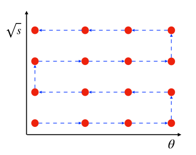
Figure 4: Schematic representation of the procedure exploited to optimise the grid construction within DiffExp. Red dots represents the points in which the MIs are evaluated and the blue dashed lines connect the sequential evaluations.

where $\theta$, $0<\theta<\pi$, is the scattering angle in the partonic center of mass frame.

Since the evaluation time, within DiffExp, for the MIs needed in this process is relatively low, we can build the grid of points as follows. We consider a total number of 13752 points in the following range for the scattering angle $\theta$ and the energy of the center of mass $s$:

$$-0.99<\cos{\theta}<0.99,\;\;\;8\operatorname{GeV}<\sqrt{s}<2.2\operatorname{TeV}.$$ (44)

The points $p_{i,j}$ of the grid are equally spaced in the coordinate system $(s,t)$ as follows:

$$p_{i,j}:=\begin{cases}s_{i}=s_{0}+(s_{f}-s_{0})\frac{i}{572}\\ t_{j}=-\frac{s_{i}}{2}(1-\cos{\theta_{j}}),\;\;\;\cos{\theta_{j}}=\cos{\theta_{0}}+(\cos{\theta_{f}}-\cos{\theta_{0}})\frac{j}{23}\end{cases}$$ (45)

where $s_{0}=64\operatorname{GeV}^{2}$, $s_{f}=4.4\operatorname{TeV}^{2}$, $\cos{\theta_{0}}=-0.99$, $\cos{\theta_{f}}=0.99$ and the indices $i,j$ take the values $i\in[0,572]$, $j\in[0,23]$. We constructed the grid by performing sequential numerical evaluations of the MIs in DiffExp as depicted schematically in figure 4. Starting from the boundary conditions for the systems of differential equations, we perform a first evaluation in the physical point $p_{0,0}$. From this point, at fixed value of $s$, we move along the $\theta$ axis, from $\cos{\theta}=-0.99$ to $\cos{\theta}=0.99$, up to the point $p_{0,23}$. Then, we increase the value of $s$ and we move in the other direction along the $\theta$ axis up to the point $p_{1,0}$, and so on so forth. In order to optimise the grid generation, for each evaluation we use as boundary conditions the value of the MIs obtained at the previous point. This procedure effectively increases the efficiency of the evaluation for the MIs. In particular, we managed to evaluate the MIs in all the points of the grid, with a 16 digits accuracy, in 2.5 hours for the system PLA and 10.5 hours for the system NPL, on a single core laptop.

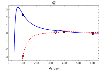
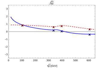
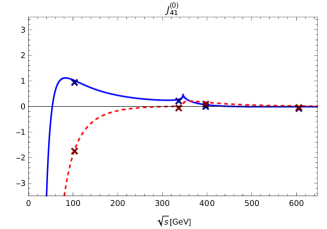
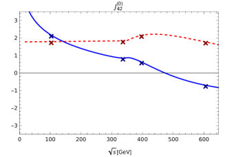
Figure 5: Numerical checks for the non-planar double-box MIs $\mathcal{J}_{39},\mathcal{J}_{40},\mathcal{J}_{41}$ and $\mathcal{J}_{42}$. The plots show the order $\mathcal{O}(\epsilon^{0})$ of the masters. Blue and dashed red lines represent, respectively, the numerical values of real and imaginary part of the MIs obtained with DiffExp. Crossed dots represent numerical values obtained with AMFlow. The evaluations are performed for different values of $\sqrt{s}$ at fixed angle $\theta$ (in this case $\cos{\theta}=0.7$).

Finally, in order to validate our results, we performed numerical checks for the MIs against independent numerical evaluations done with the AMFlow package Liu_2023 , which implements the auxiliary mass flow method Liu:2017jxz ; Liu:2021wks . The MIs have been checked for several points in the physical phase-space region, finding an agreement between the two independent evaluations up to 200 digits of accuracy. As a proof of concept of the numerical checks we show in figure 5 our results for the double-box MIs in the non-planar topology NPL.

4 Conclusions

In this paper we presented the computation of the two-loop form factors for diphoton production in the $q\bar{q}$ channel, where the full dependence on the top quark mass has been retained. This computation represents the only missing ingredient, at two loops, in order to be able to perform a phenomenological study for diphoton production at NNLO Becchetti:ta which fully takes into account the dependence on the top quark mass in all the relevant channels.

The non-planar topology which contributes to this process contains two sectors of MIs whose analytic representation cannot be given in terms of MPLs. In order to be able to exploit our results for phenomenological applications, we computed the MIs by means of differential equations, exploiting the generalised power series technique. This method proves to be of great use for phenomenological applications, especially in cases where the functional space for the MIs contains not only polylogarithmic functions.

Appendix A The master integrals

The MIs appearing in the form factors, modulo permutations of the external momenta, are the following:

$$\mathcal{J}_{1} =\mathcal{I}_{\text{PLA}}(0,0,0,2,0,0,2,0,0),\hskip 28.45274pt\mathcal{J}_{2}(y)=\mathcal{I}_{\text{PLA}}(0,1,2,0,0,0,2,0,0),$$

$$\mathcal{J}_{3}(y) =\mathcal{I}_{\text{PLA}}(0,0,0,2,1,2,0,0,0),\hskip 28.45274pt\mathcal{J}_{4}(y)=\mathcal{I}_{\text{PLA}}(0,0,2,1,2,0,0,0,0),$$

$$\mathcal{J}_{5}(y) =\mathcal{I}_{\text{PLA}}(0,0,1,2,2,0,0,0,0),\hskip 28.45274pt\mathcal{J}_{6}(y)=\mathcal{I}_{\text{PLA}}(0,1,2,0,2,1,0,0,0),$$

$$\mathcal{J}_{7}(y) =\mathcal{I}_{\text{PLA}}(0,0,0,2,1,1,1,0,0),\hskip 28.45274pt\mathcal{J}_{8}(y)=\mathcal{I}_{\text{PLA}}(0,0,1,3,1,0,1,0,0),$$

$$\mathcal{J}_{9}(y) =\mathcal{I}_{\text{PLA}}(0,1,1,2,0,0,1,0,0),\hskip 28.45274pt\mathcal{J}_{10}(y)=\mathcal{I}_{\text{PLA}}(0,1,2,1,0,0,2,0,0),$$

$$\mathcal{J}_{11}(y) =\mathcal{I}_{\text{PLA}}(1,0,0,2,1,1,0,0,0),\hskip 28.45274pt\mathcal{J}_{12}(y)=\mathcal{I}_{\text{PLA}}(2,0,0,1,1,1,0,0,0),$$

$$\mathcal{J}_{13}(y) =\mathcal{I}_{\text{PLA}}(1,0,0,2,1,2,0,0,0),\hskip 28.45274pt\mathcal{J}_{14}(y)=\mathcal{I}_{\text{PLA}}(0,1,1,1,1,1,0,0,0),$$

$$\mathcal{J}_{15}(y) =\mathcal{I}_{\text{PLA}}(0,2,1,0,1,1,1,0,0),\hskip 28.45274pt\mathcal{J}_{16}(y)=\mathcal{I}_{\text{PLA}}(0,1,1,1,0,1,1,0,0),$$

$$\mathcal{J}_{17}(y) =\mathcal{I}_{\text{NPL}}(0,1,0,1,1,1,1,0,0),\hskip 28.45274pt\mathcal{J}_{18}(y)=\mathcal{I}_{\text{PLA}}(0,1,1,1,1,1,1,0,0),$$

$$\mathcal{J}_{19}(y) =\mathcal{I}_{\text{NPL}}(0,1,1,1,1,1,1,0,0),\hskip 28.45274pt\mathcal{J}_{20}(y)=\mathcal{I}_{\text{NPL}}(0,1,1,2,1,1,1,0,0),$$

$$\mathcal{J}_{21}(y,z) =\mathcal{I}_{\text{PLB}}(1,1,1,2,0,1,0,0,0),\hskip 28.45274pt\mathcal{J}_{22}(y,z)=\mathcal{I}_{\text{PLA}}(1,1,1,2,0,0,1,0,0),$$

$$\mathcal{J}_{23}(y,z) =\mathcal{I}_{\text{PLA}}(1,1,1,2,0,0,1,-1,0),\hskip 19.91684pt\mathcal{J}_{24}(y,z)=\mathcal{I}_{\text{PLA}}(1,0,1,1,1,0,1,0,0),$$

$$\mathcal{J}_{25}(y,z) =\mathcal{I}_{\text{PLA}}(1,0,1,2,1,0,1,0,0),\hskip 28.45274pt\mathcal{J}_{26}(y,z)=\mathcal{I}_{\text{PLA}}(1,0,0,2,1,1,1,0,0),$$

$$\mathcal{J}_{27}(y,z) =\mathcal{I}_{\text{PLA}}(1,0,0,3,1,1,1,0,0),\hskip 28.45274pt\mathcal{J}_{28}(y,z)=\mathcal{I}_{\text{PLA}}(1,0,0,2,1,1,1,0,-1),$$

$$\mathcal{J}_{29}(y,z) =\mathcal{I}_{\text{PLA}}(1,1,1,1,1,0,1,0,0),\hskip 28.45274pt\mathcal{J}_{30}(y,z)=\mathcal{I}_{\text{NPL}}(1,0,0,1,1,1,1,0,0),$$

$$\mathcal{J}_{31}(y,z) =\mathcal{I}_{\text{NPL}}(2,0,0,1,1,1,1,0,0),\hskip 28.45274pt\mathcal{J}_{32}(y,z)=\mathcal{I}_{\text{NPL}}(1,0,0,1,2,1,1,0,0),$$

$$\mathcal{J}_{33}(y,z) =\mathcal{I}_{\text{NPL}}(1,1,0,1,1,1,1,0,0),\hskip 28.45274pt\mathcal{J}_{34}(y,z)=\mathcal{I}_{\text{NPL}}(1,1,0,2,1,1,1,0,0),$$

$$\mathcal{J}_{35}(y,z) =\mathcal{I}_{\text{PLA}}(1,1,1,1,1,1,1,0,0),\hskip 28.45274pt\mathcal{J}_{36}(y,z)=\mathcal{I}_{\text{PLA}}(1,1,1,1,1,1,1,-1,0),$$

$$\mathcal{J}_{37}(y,z) =\mathcal{I}_{\text{PLA}}(1,1,1,1,1,1,1,0,-1),\hskip 19.91684pt\mathcal{J}_{38}(y,z)=\mathcal{I}_{\text{PLA}}(1,1,1,1,1,1,1,-1,-1),$$

$$\mathcal{J}_{39}(y,z) =\mathcal{I}_{\text{NPL}}(1,1,1,1,1,1,1,0,0),\hskip 28.45274pt\mathcal{J}_{40}(y,z)=\mathcal{I}_{\text{NPL}}(1,1,1,1,1,1,1,-1,0),$$

$$\mathcal{J}_{41}(y,z) =\mathcal{I}_{\text{NPL}}(1,1,1,1,2,1,1,0,0),\hskip 28.45274pt\mathcal{J}_{42}(y,z)=\mathcal{I}_{\text{NPL}}(1,1,1,1,1,1,1,-1,-1).$$

To complete the whole set of MIs appearing in the form factors, we have to consider also the following masters, obtained from the previous list permuting the kinematic variables ($y$,$z$ and $w=-y-z$):

$$\mathcal{J}_{43}(z) =\mathcal{J}_{2}(z),\hskip 45.52458pt\mathcal{J}_{44}(w)=\mathcal{J}_{2}(w),$$

$$\mathcal{J}_{45}(w) =\mathcal{J}_{4}(w),\hskip 45.52458pt\mathcal{J}_{46}(z)=\mathcal{J}_{4}(z),$$

$$\mathcal{J}_{47}(w) =\mathcal{J}_{5}(w),\hskip 45.52458pt\mathcal{J}_{48}(z)=\mathcal{J}_{5}(z),$$

$$\mathcal{J}_{49}(w) =\mathcal{J}_{8}(w),\hskip 45.52458pt\mathcal{J}_{50}(z)=\mathcal{J}_{8}(z),$$

$$\mathcal{J}_{51}(y,z) =\mathcal{J}_{21}(y,w),\hskip 28.45274pt\mathcal{J}_{52}(y,z)=\mathcal{J}_{22}(y,w),$$

$$\mathcal{J}_{53}(y,z) =\mathcal{J}_{23}(y,w),\hskip 28.45274pt\mathcal{J}_{54}(y,z)=\mathcal{J}_{24}(y,w),$$

$$\mathcal{J}_{55}(y,z) =\mathcal{J}_{25}(y,w),\hskip 28.45274pt\mathcal{J}_{56}(y,z)=\mathcal{J}_{26}(y,w),$$

$$\mathcal{J}_{57}(y,z) =\mathcal{J}_{27}(y,w),\hskip 28.45274pt\mathcal{J}_{58}(y,z)=\mathcal{J}_{28}(y,w),$$

$$\mathcal{J}_{59}(y,z) =\mathcal{J}_{29}(y,w),\hskip 28.45274pt\mathcal{J}_{60}(y,z)=\mathcal{J}_{30}(y,w),$$

$$\mathcal{J}_{61}(y,z) =\mathcal{J}_{31}(y,w),\hskip 28.45274pt\mathcal{J}_{62}(y,z)=\mathcal{J}_{32}(y,w),$$

$$\mathcal{J}_{63}(y,z) =\mathcal{J}_{33}(y,w),\hskip 28.45274pt\mathcal{J}_{64}(y,z)=\mathcal{J}_{34}(y,w),$$

$$\mathcal{J}_{65}(y,z) =\mathcal{J}_{35}(y,w),\hskip 28.45274pt\mathcal{J}_{66}(y,z)=\mathcal{J}_{36}(y,w),$$

$$\mathcal{J}_{67}(y,z) =\mathcal{J}_{37}(y,w),\hskip 28.45274pt\mathcal{J}_{68}(y,z)=\mathcal{J}_{38}(y,w),$$

$$\mathcal{J}_{69}(y,z) =\mathcal{J}_{39}(y,w),\hskip 28.45274pt\mathcal{J}_{70}(y,z)=\mathcal{J}_{40}(y,w),$$

$$\mathcal{J}_{71}(y,z) =\mathcal{J}_{41}(y,w),\hskip 28.45274pt\mathcal{J}_{72}(y,z)=\mathcal{J}_{42}(y,w).$$

References

- (1) M. Becchetti, R. Bonciani, L. Cieri, F. Coro and F. Ripani, Full top-quark mass dependence in diphoton production at NNLO in QCD, 2308.10885.
- (2) ATLAS collaboration, G. Aad et al., Measurement of the production cross section of pairs of isolated photons in collisions at 13 TeV with the ATLAS detector, JHEP 11 (2021) 169, [2107.09330].
- (3) ATLAS collaboration, M. Aaboud et al., Measurements of integrated and differential cross sections for isolated photon pair production in collisions at TeV with the ATLAS detector, Phys. Rev. D 95 (2017) 112005, [1704.03839].
- (4) CMS collaboration, S. Chatrchyan et al., Measurement of differential cross sections for the production of a pair of isolated photons in pp collisions at , Eur. Phys. J. C 74 (2014) 3129, [1405.7225].
- (5) ATLAS collaboration, G. Aad et al., Measurement of isolated-photon pair production in collisions at TeV with the ATLAS detector, JHEP 01 (2013) 086, [1211.1913].
- (6) ATLAS collaboration, G. Aad et al., Search for periodic signals in the dielectron and diphoton invariant mass spectra using 139 fb-1 of collisions at 13 TeV with the ATLAS detector, 2305.10894.
- (7) ATLAS collaboration, G. Aad et al., Search in diphoton and dielectron final states for displaced production of Higgs or Z bosons with the ATLAS detector in s=13 TeV pp collisions, Phys. Rev. D 108 (2023) 012012, [2304.12885].
- (8) ATLAS collaboration, G. Aad et al., Search for boosted diphoton resonances in the 10 to 70 GeV mass range using 138 fb-1 of 13 TeV pp collisions with the ATLAS detector, JHEP 07 (2023) 155, [2211.04172].
- (9) CMS collaboration, A. M. Sirunyan et al., Search for supersymmetry using Higgs boson to diphoton decays at = 13 TeV, JHEP 11 (2019) 109, [1908.08500].
- (10) CMS collaboration, V. Khachatryan et al., Search for high-mass diphoton resonances in proton–proton collisions at 13 TeV and combination with 8 TeV search, Phys. Lett. B 767 (2017) 147–170, [1609.02507].
- (11) ATLAS collaboration, M. Aaboud et al., Search for new phenomena in high-mass diphoton final states using 37 fb-1 of proton–proton collisions collected at TeV with the ATLAS detector, Phys. Lett. B 775 (2017) 105–125, [1707.04147].
- (12) ATLAS collaboration, G. Aad et al., Measurements of the Higgs boson inclusive and differential fiducial cross-sections in the diphoton decay channel with pp collisions at = 13 TeV with the ATLAS detector, JHEP 08 (2022) 027, [2202.00487].
- (13) CMS collaboration, A. Tumasyan et al., Measurement of the Higgs boson inclusive and differential fiducial production cross sections in the diphoton decay channel with pp collisions at = 13 TeV, JHEP 07 (2023) 091, [2208.12279].
- (14) CMS collaboration, A. M. Sirunyan et al., Measurements of Higgs boson production cross sections and couplings in the diphoton decay channel at = 13 TeV, JHEP 07 (2021) 027, [2103.06956].
- (15) CMS collaboration, A. M. Sirunyan et al., A measurement of the Higgs boson mass in the diphoton decay channel, Phys. Lett. B 805 (2020) 135425, [2002.06398].
- (16) ATLAS collaboration, M. Aaboud et al., Measurements of Higgs boson properties in the diphoton decay channel with 36 fb-1 of collision data at TeV with the ATLAS detector, Phys. Rev. D 98 (2018) 052005, [1802.04146].
- (17) CMS collaboration, V. Khachatryan et al., Observation of the Diphoton Decay of the Higgs Boson and Measurement of Its Properties, Eur. Phys. J. C 74 (2014) 3076, [1407.0558].
- (18) ATLAS collaboration, G. Aad et al., Measurement of Higgs boson production in the diphoton decay channel in pp collisions at center-of-mass energies of 7 and 8 TeV with the ATLAS detector, Phys. Rev. D 90 (2014) 112015, [1408.7084].
- (19) ATLAS collaboration, G. Aad et al., Measurements of fiducial and differential cross sections for Higgs boson production in the diphoton decay channel at TeV with ATLAS, JHEP 09 (2014) 112, [1407.4222].
- (20) ATLAS collaboration, G. Aad et al., Observation of a new particle in the search for the Standard Model Higgs boson with the ATLAS detector at the LHC, Phys. Lett. B 716 (2012) 1–29, [1207.7214].
- (21) CMS collaboration, S. Chatrchyan et al., Observation of a New Boson at a Mass of 125 GeV with the CMS Experiment at the LHC, Phys. Lett. B 716 (2012) 30–61, [1207.7235].
- (22) S. Catani, L. Cieri, D. de Florian, G. Ferrera and M. Grazzini, Diphoton production at hadron colliders: a fully-differential QCD calculation at NNLO, Phys. Rev. Lett. 108 (2012) 072001, [1110.2375].
- (23) J. M. Campbell, R. K. Ellis, Y. Li and C. Williams, Predictions for diphoton production at the LHC through NNLO in QCD, JHEP 07 (2016) 148, [1603.02663].
- (24) S. Catani, L. Cieri, D. de Florian, G. Ferrera and M. Grazzini, Diphoton production at the LHC: a QCD study up to NNLO, JHEP 04 (2018) 142, [1802.02095].
- (25) R. Schuermann, X. Chen, T. Gehrmann, E. W. N. Glover, M. Höfer and A. Huss, NNLO Photon Production with Realistic Photon Isolation, PoS LL2022 (2022) 034, [2208.02669].
- (26) L. Ametller, E. Gava, N. Paver and D. Treleani, Role of the QCD Induced Gluon - Gluon Coupling to Gauge Boson Pairs in the Multi - Tev Region, Phys. Rev. D 32 (1985) 1699.
- (27) S. J. Parke and T. R. Taylor, An Amplitude for Gluon Scattering, Phys. Rev. Lett. 56 (1986) 2459.
- (28) D. A. Dicus and S. S. D. Willenbrock, Photon Pair Production and the Intermediate Mass Higgs Boson, Phys. Rev. D 37 (1988) 1801.
- (29) V. D. Barger, T. Han, J. Ohnemus and D. Zeppenfeld, Pair Production of W±, and Z in Association With Jets, Phys. Rev. D 41 (1990) 2782.
- (30) M. L. Mangano and S. J. Parke, Multiparton amplitudes in gauge theories, Phys. Rept. 200 (1991) 301–367, [hep-th/0509223].
- (31) Z. Bern, L. J. Dixon and D. A. Kosower, One loop corrections to two quark three gluon amplitudes, Nucl. Phys. B 437 (1995) 259–304, [hep-ph/9409393].
- (32) A. Signer, One loop corrections to five parton amplitudes with external photons, Phys. Lett. B 357 (1995) 204–210, [hep-ph/9507442].
- (33) C. Balazs, E. L. Berger, S. Mrenna and C. P. Yuan, Photon pair production with soft gluon resummation in hadronic interactions, Phys. Rev. D 57 (1998) 6934–6947, [hep-ph/9712471].
- (34) V. Del Duca, W. B. Kilgore and F. Maltoni, Multiphoton amplitudes for next-to-leading order QCD, Nucl. Phys. B 566 (2000) 252–274, [hep-ph/9910253].
- (35) C. Anastasiou, E. W. N. Glover and M. E. Tejeda-Yeomans, Two loop QED and QCD corrections to massless fermion boson scattering, Nucl. Phys. B 629 (2002) 255–289, [hep-ph/0201274].
- (36) V. Del Duca, F. Maltoni, Z. Nagy and Z. Trocsanyi, QCD radiative corrections to prompt diphoton production in association with a jet at hadron colliders, JHEP 04 (2003) 059, [hep-ph/0303012].
- (37) F. Caola, A. Chakraborty, G. Gambuti, A. von Manteuffel and L. Tancredi, Three-loop helicity amplitudes for quark-gluon scattering in QCD, JHEP 12 (2022) 082, [2207.03503].
- (38) H. A. Chawdhry, M. Czakon, A. Mitov and R. Poncelet, Two-loop leading-color helicity amplitudes for three-photon production at the LHC, JHEP 06 (2021) 150, [2012.13553].
- (39) B. Agarwal, F. Buccioni, A. von Manteuffel and L. Tancredi, Two-loop leading colour QCD corrections to and , JHEP 04 (2021) 201, [2102.01820].
- (40) H. A. Chawdhry, M. Czakon, A. Mitov and R. Poncelet, Two-loop leading-colour QCD helicity amplitudes for two-photon plus jet production at the LHC, JHEP 07 (2021) 164, [2103.04319].
- (41) B. Agarwal, F. Buccioni, A. von Manteuffel and L. Tancredi, Two-Loop Helicity Amplitudes for Diphoton Plus Jet Production in Full Color, Phys. Rev. Lett. 127 (2021) 262001, [2105.04585].
- (42) Z. Bern, A. De Freitas and L. J. Dixon, Two loop amplitudes for gluon fusion into two photons, JHEP 09 (2001) 037, [hep-ph/0109078].
- (43) H. A. Chawdhry, M. Czakon, A. Mitov and R. Poncelet, NNLO QCD corrections to diphoton production with an additional jet at the LHC, JHEP 09 (2021) 093, [2105.06940].
- (44) F. Maltoni, M. K. Mandal and X. Zhao, Top-quark effects in diphoton production through gluon fusion at next-to-leading order in QCD, Phys. Rev. D 100 (2019) 071501, [1812.08703].
- (45) L. Chen, G. Heinrich, S. Jahn, S. P. Jones, M. Kerner, J. Schlenk et al., Photon pair production in gluon fusion: Top quark effects at NLO with threshold matching, JHEP 04 (2020) 115, [1911.09314].
- (46) T. Peraro and L. Tancredi, Tensor decomposition for bosonic and fermionic scattering amplitudes, Phys. Rev. D 103 (2021) 054042, [2012.00820].
- (47) K. G. Chetyrkin, A. L. Kataev and F. V. Tkachov, Higher Order Corrections to Sigma-t (e+ e- — Hadrons) in Quantum Chromodynamics, Phys. Lett. B 85 (1979) 277–279.
- (48) K. G. Chetyrkin and F. V. Tkachov, Integration by Parts: The Algorithm to Calculate beta Functions in 4 Loops, Nucl. Phys. B 192 (1981) 159–204.
- (49) S. Laporta, High precision calculation of multiloop Feynman integrals by difference equations, Int.J.Mod.Phys. A15 (2000) 5087–5159, [hep-ph/0102033].
- (50) C. Anastasiou and A. Lazopoulos, Automatic integral reduction for higher order perturbative calculations, JHEP 07 (2004) 046, [hep-ph/0404258].
- (51) C. Studerus, Reduze-Feynman Integral Reduction in C++, Comput.Phys.Commun. 181 (2010) 1293–1300, [0912.2546].
- (52) A. von Manteuffel and C. Studerus, Reduze 2 - Distributed Feynman Integral Reduction, 1201.4330.
- (53) R. N. Lee, Presenting LiteRed: a tool for the Loop InTEgrals REDuction, 1212.2685.
- (54) R. N. Lee, LiteRed 1.4: a powerful tool for reduction of multiloop integrals, J. Phys. Conf. Ser. 523 (2014) 012059, [1310.1145].
- (55) A. V. Smirnov, Algorithm FIRE – Feynman Integral REduction, JHEP 10 (2008) 107, [0807.3243].
- (56) A. V. Smirnov, FIRE5: a C++ implementation of Feynman Integral REduction, Comput. Phys. Commun. 189 (2014) 182–191, [1408.2372].
- (57) P. Maierhöfer, J. Usovitsch and P. Uwer, Kira—A Feynman integral reduction program, Comput. Phys. Commun. 230 (2018) 99–112, [1705.05610].
- (58) J. Klappert, F. Lange, P. Maierhöfer and J. Usovitsch, Integral reduction with Kira 2.0 and finite field methods, Comput. Phys. Commun. 266 (2021) 108024, [2008.06494].
- (59) A. V. Kotikov, Differential equations method: New technique for massive Feynman diagrams calculation, Phys. Lett. B 254 (1991) 158–164.
- (60) A. V. Kotikov, Differential equation method: The Calculation of N point Feynman diagrams, Phys. Lett. B 267 (1991) 123–127.
- (61) Z. Bern, L. J. Dixon and D. A. Kosower, Dimensionally regulated pentagon integrals, Nucl. Phys. B 412 (1994) 751–816, [hep-ph/9306240].
- (62) E. Remiddi, Differential equations for Feynman graph amplitudes, Nuovo Cim. A 110 (1997) 1435–1452, [hep-th/9711188].
- (63) T. Gehrmann and E. Remiddi, Differential equations for two loop four point functions, Nucl. Phys. B 580 (2000) 485–518, [hep-ph/9912329].
- (64) M. Argeri and P. Mastrolia, Feynman Diagrams and Differential Equations, Int. J. Mod. Phys. A 22 (2007) 4375–4436, [0707.4037].
- (65) J. M. Henn, Multiloop integrals in dimensional regularization made simple, Phys. Rev. Lett. 110 (2013) 251601, [1304.1806].
- (66) J. M. Henn, Lectures on differential equations for Feynman integrals, J. Phys. A 48 (2015) 153001, [1412.2296].
- (67) M. Becchetti and R. Bonciani, Two-Loop Master Integrals for the Planar QCD Massive Corrections to Di-photon and Di-jet Hadro-production, JHEP 01 (2018) 048, [1712.02537].
- (68) S. Caron-Huot and J. M. Henn, Iterative structure of finite loop integrals, JHEP 06 (2014) 114, [1404.2922].
- (69) R. Bonciani, P. Mastrolia and E. Remiddi, Vertex diagrams for the QED form-factors at the two loop level, Nucl. Phys. B 661 (2003) 289–343, [hep-ph/0301170].
- (70) U. Aglietti and R. Bonciani, Master integrals with 2 and 3 massive propagators for the 2 loop electroweak form-factor - planar case, Nucl. Phys. B 698 (2004) 277–318, [hep-ph/0401193].
- (71) R. Bonciani, P. Mastrolia and E. Remiddi, Master integrals for the two loop QCD virtual corrections to the forward backward asymmetry, Nucl. Phys. B 690 (2004) 138–176, [hep-ph/0311145].
- (72) R. Bonciani, A. Ferroglia and A. A. Penin, Heavy-flavor contribution to Bhabha scattering, Phys. Rev. Lett. 100 (2008) 131601, [0710.4775].
- (73) R. Bonciani, A. Ferroglia and A. A. Penin, Calculation of the Two-Loop Heavy-Flavor Contribution to Bhabha Scattering, JHEP 02 (2008) 080, [0802.2215].
- (74) A. B. Goncharov, Multiple polylogarithms and mixed Tate motives, math/0103059.
- (75) A. B. Goncharov, Multiple polylogarithms, cyclotomy and modular complexes, Math. Res. Lett. 5 (1998) 497–516, [1105.2076].
- (76) A. Goncharov, Multiple polylogarithms and mixed Tate motives, math/0103059.
- (77) E. Remiddi and J. A. M. Vermaseren, Harmonic polylogarithms, Int. J. Mod. Phys. A 15 (2000) 725–754, [hep-ph/9905237].
- (78) J. Vollinga and S. Weinzierl, Numerical evaluation of multiple polylogarithms, Comput. Phys. Commun. 167 (2005) 177, [hep-ph/0410259].
- (79) C. Duhr and F. Dulat, PolyLogTools — polylogs for the masses, JHEP 08 (2019) 135, [1904.07279].
- (80) L. Adams, E. Chaubey and S. Weinzierl, Simplifying Differential Equations for Multiscale Feynman Integrals beyond Multiple Polylogarithms, Phys. Rev. Lett. 118 (2017) 141602, [1702.04279].
- (81) F. C. S. Brown and A. Levin, Multiple elliptic polylogarithms, 2013.
- (82) J. Broedel, C. R. Mafra, N. Matthes and O. Schlotterer, Elliptic multiple zeta values and one-loop superstring amplitudes, JHEP 07 (2015) 112, [1412.5535].
- (83) J. Broedel, C. Duhr, F. Dulat and L. Tancredi, Elliptic polylogarithms and iterated integrals on elliptic curves. Part I: general formalism, JHEP 05 (2018) 093, [1712.07089].
- (84) Y. I. Manin, Iterated integrals of modular forms and noncommutative modular symbols, in Algebraic geometry and number theory, vol. 253 of Progr. Math., (Boston), pp. 565–597, Birkhäuser Boston, 2006. math/0502576.
- (85) F. Brown, Multiple modular values and the relative completion of the fundamental group of , 1407.5167v4.
- (86) L. Adams, C. Bogner and S. Weinzierl, The two-loop sunrise graph in two space-time dimensions with arbitrary masses in terms of elliptic dilogarithms, J. Math. Phys. 55 (2014) 102301, [1405.5640].
- (87) H. Frellesvig, On epsilon factorized differential equations for elliptic Feynman integrals, JHEP 03 (2022) 079, [2110.07968].
- (88) H. Frellesvig and S. Weinzierl, On -factorised bases and pure Feynman integrals, 2301.02264.
- (89) L. Görges, C. Nega, L. Tancredi and F. J. Wagner, On a procedure to derive -factorised differential equations beyond polylogarithms, 2305.14090.
- (90) C. Duhr, A. Klemm, F. Loebbert, C. Nega and F. Porkert, Yangian-Invariant Fishnet Integrals in Two Dimensions as Volumes of Calabi-Yau Varieties, Phys. Rev. Lett. 130 (2023) 041602, [2209.05291].
- (91) C. Duhr, A. Klemm, C. Nega and L. Tancredi, The ice cone family and iterated integrals for Calabi-Yau varieties, JHEP 02 (2023) 228, [2212.09550].
- (92) J. L. Bourjaily et al., Functions Beyond Multiple Polylogarithms for Precision Collider Physics, in Snowmass 2021, 3, 2022. 2203.07088.
- (93) S. Abreu, M. Becchetti, C. Duhr and M. A. Ozcelik, Two-loop master integrals for pseudo-scalar quarkonium and leptonium production and decay, JHEP 09 (2022) 194, [2206.03848].
- (94) S. Abreu, M. Becchetti, C. Duhr and M. A. Ozcelik, Two-loop form factors for pseudo-scalar quarkonium production and decay, JHEP 02 (2023) 250, [2211.08838].
- (95) S. Pozzorini and E. Remiddi, Precise numerical evaluation of the two loop sunrise graph master integrals in the equal mass case, Comput. Phys. Commun. 175 (2006) 381–387, [hep-ph/0505041].
- (96) U. Aglietti, R. Bonciani, L. Grassi and E. Remiddi, The Two loop crossed ladder vertex diagram with two massive exchanges, Nucl. Phys. B 789 (2008) 45–83, [0705.2616].
- (97) R. Bonciani, G. Degrassi, P. P. Giardino and R. Gröber, A Numerical Routine for the Crossed Vertex Diagram with a Massive-Particle Loop, Comput. Phys. Commun. 241 (2019) 122–131, [1812.02698].
- (98) R. N. Lee, A. V. Smirnov and V. A. Smirnov, Solving differential equations for Feynman integrals by expansions near singular points, JHEP 03 (2018) 008, [1709.07525].
- (99) M. K. Mandal and X. Zhao, Evaluating multi-loop Feynman integrals numerically through differential equations, JHEP 03 (2019) 190, [1812.03060].
- (100) F. Moriello, Generalised power series expansions for the elliptic planar families of Higgs + jet production at two loops, JHEP 01 (2020) 150, [1907.13234].
- (101) R. Bonciani, V. Del Duca, H. Frellesvig, J. M. Henn, M. Hidding, L. Maestri et al., Evaluating a family of two-loop non-planar master integrals for Higgs + jet production with full heavy-quark mass dependence, JHEP 01 (2020) 132, [1907.13156].
- (102) M. Hidding, DiffExp, a Mathematica package for computing Feynman integrals in terms of one-dimensional series expansions, Comput. Phys. Commun. 269 (2021) 108125, [2006.05510].
- (103) T. Armadillo, R. Bonciani, S. Devoto, N. Rana and A. Vicini, Evaluation of Feynman integrals with arbitrary complex masses via series expansions, Comput. Phys. Commun. 282 (2023) 108545, [2205.03345].
- (104) M. Becchetti, R. Bonciani, V. Del Duca, V. Hirschi, F. Moriello and A. Schweitzer, Next-to-leading order corrections to light-quark mixed QCD-EW contributions to Higgs boson production, Phys. Rev. D 103 (2021) 054037, [2010.09451].
- (105) R. Bonciani, L. Buonocore, M. Grazzini, S. Kallweit, N. Rana, F. Tramontano et al., Mixed Strong-Electroweak Corrections to the Drell-Yan Process, Phys. Rev. Lett. 128 (2022) 012002, [2106.11953].
- (106) R. Bonciani, V. Del Duca, H. Frellesvig, M. Hidding, V. Hirschi, F. Moriello et al., Next-to-leading-order QCD corrections to Higgs production in association with a jet, Phys. Lett. B 843 (2023) 137995, [2206.10490].
- (107) M. J. G. Veltman, Diagrammatica: The Path to Feynman rules, vol. 4. Cambridge University Press, 5, 2012.
- (108) T. Hahn, Generating Feynman diagrams and amplitudes with FeynArts 3, Comput. Phys. Commun. 140 (2001) 418–431, [hep-ph/0012260].
- (109) T. Peraro, FiniteFlow: multivariate functional reconstruction using finite fields and dataflow graphs, JHEP 07 (2019) 031, [1905.08019].
- (110) U. Aglietti, R. Bonciani, G. Degrassi and A. Vicini, Analytic Results for Virtual QCD Corrections to Higgs Production and Decay, JHEP 01 (2007) 021, [hep-ph/0611266].
- (111) C. Anastasiou, S. Beerli, S. Bucherer, A. Daleo and Z. Kunszt, Two-loop amplitudes and master integrals for the production of a Higgs boson via a massive quark and a scalar-quark loop, JHEP 01 (2007) 082, [hep-ph/0611236].
- (112) A. von Manteuffel and L. Tancredi, A non-planar two-loop three-point function beyond multiple polylogarithms, JHEP 06 (2017) 127, [1701.05905].
- (113) S. Catani and M. Grazzini, An NNLO subtraction formalism in hadron collisions and its application to Higgs boson production at the LHC, Phys. Rev. Lett. 98 (2007) 222002, [hep-ph/0703012].
- (114) S. Catani, L. Cieri, D. de Florian, G. Ferrera and M. Grazzini, Universality of transverse-momentum resummation and hard factors at the NNLO, Nucl. Phys. B 881 (2014) 414–443, [1311.1654].
- (115) G. Bozzi, S. Catani, D. de Florian and M. Grazzini, Transverse-momentum resummation and the spectrum of the Higgs boson at the LHC, Nucl. Phys. B 737 (2006) 73–120, [hep-ph/0508068].
- (116) J. Kuipers, T. Ueda, J. A. M. Vermaseren and J. Vollinga, FORM version 4.0, Comput. Phys. Commun. 184 (2013) 1453–1467, [1203.6543].
- (117) B. Ruijl, T. Ueda and J. Vermaseren, FORM version 4.2, 1707.06453.
- (118) P. Bärnreuther, M. Czakon and P. Fiedler, Virtual amplitudes and threshold behaviour of hadronic top-quark pair-production cross sections, JHEP 02 (2014) 078, [1312.6279].
- (119) D. J. Broadhurst, J. Fleischer and O. V. Tarasov, Two loop two point functions with masses: Asymptotic expansions and Taylor series, in any dimension, Z. Phys. C 60 (1993) 287–302, [hep-ph/9304303].
- (120) K. Melnikov and T. v. Ritbergen, The Three loop relation between the MS-bar and the pole quark masses, Phys. Lett. B 482 (2000) 99–108, [hep-ph/9912391].
- (121) A. Mitov and S. Moch, The Singular behavior of massive QCD amplitudes, JHEP 05 (2007) 001, [hep-ph/0612149].
- (122) A. B. Goncharov, M. Spradlin, C. Vergu and A. Volovich, Classical Polylogarithms for Amplitudes and Wilson Loops, Phys. Rev. Lett. 105 (2010) 151605, [1006.5703].
- (123) C. Duhr, H. Gangl and J. R. Rhodes, From polygons and symbols to polylogarithmic functions, JHEP 10 (2012) 075, [1110.0458].
- (124) J. M. Henn, Lectures on differential equations for feynman integrals, Journal of Physics A: Mathematical and Theoretical 48 (mar, 2015) 153001.
- (125) X. Liu and Y.-Q. Ma, AMFlow: A mathematica package for feynman integrals computation via auxiliary mass flow, Computer Physics Communications 283 (feb, 2023) 108565.
- (126) J. Broedel, C. Duhr, F. Dulat, B. Penante and L. Tancredi, Elliptic polylogarithms and Feynman parameter integrals, JHEP 05 (2019) 120, [1902.09971].
- (127) H. Frellesvig and C. G. Papadopoulos, Cuts of Feynman Integrals in Baikov representation, JHEP 04 (2017) 083, [1701.07356].
- (128) M. Harley, F. Moriello and R. M. Schabinger, Baikov-Lee Representations Of Cut Feynman Integrals, JHEP 06 (2017) 049, [1705.03478].
- (129) P. A. Baikov, Explicit solutions of n loop vacuum integral recurrence relations, hep-ph/9604254.
- (130) C. Dlapa, Algorithms and techniques for finding canonical differential equations of Feynman integrals. PhD thesis, Munich U., 2022. 10.5282/edoc.29769.
- (131) F. Cachazo, Sharpening The Leading Singularity, 0803.1988.
- (132) X. Liu, Y.-Q. Ma and C.-Y. Wang, A Systematic and Efficient Method to Compute Multi-loop Master Integrals, Phys. Lett. B 779 (2018) 353–357, [1711.09572].
- (133) X. Liu and Y.-Q. Ma, Multiloop corrections for collider processes using auxiliary mass flow, Phys. Rev. D 105 (2022) L051503, [2107.01864].