Attitude Determination in Urban Canyons: A Synergy between GNSS and 5G Observations

biography

Pinjun Zhengis a PhD student with the Electrical and Computer Engineering Program, King Abdullah University of Science and Technology (KAUST), Thuwal, Saudi Arabia. His current research focuses on mmWave/THz localization and communications.

Xing Liuis a postdoctoral researcher with the Electrical and Computer Engineering Program, King Abdullah University of Science and Technology (KAUST), Thuwal, Saudi Arabia. His current research focuses on precise GNSS positioning and attitude determination.

Tarig Ballalis a research scientist with the Electrical and Computer Engineering Program, King Abdullah University of Science and Technology (KAUST), Thuwal, Saudi Arabia. His research interests lie in the areas of signal and image processing, localization and tracking, in addition to GNSS positioning and attitude determination.

Tareq Y. Al-Naffouriis a professor with the Electrical and Computer Engineering Program, King Abdullah University of Science and Technology (KAUST), Thuwal, Saudi Arabia. His current research focuses on the areas of sparse, adaptive, and statistical signal processing and their applications, as well as machine learning and network information theory.

Abstract

This paper considers the attitude determination problem based on the global navigation satellite system (GNSS) and fifth generation (5G) measurement fusion to address the shortcomings of standalone GNSS and 5G techniques in deep urban regions. The tight fusion of the GNSS and the 5G observations results in a unique hybrid integer- and orthonormality-constrained optimization problem. To solve this problem, we propose an estimation method consisting of the steps of float solution computation, ambiguity resolution, and fixed solution computation. Numerical results reveal that the proposed method can effectively improve the attitude determination accuracy and reliability compared to either the pure GNSS solution or the pure 5G solution.

1 INTRODUCTION

With numerous emerging technologies flourishing in areas such as wireless communications, robotics, and artificial intelligence, many facets of human society are benefiting from intelligent location/attitude-aware services (Di Taranto et al.,, 2014; Alletto et al.,, 2016; Jiang et al.,, 2021). Beyond the location information, determining the user’s attitude information becomes more and more important nowadays (Douik et al.,, 2020; Liu et al.,, 2023). GNSS attitude determination has been widely studied in literature (Giorgi and Teunissen,, 2010; Teunissen,, 2012; Liu et al., 2022b, ; Liu et al.,, 2020; Liu et al., 2022a, ; Liu,, 2023). Compared to other existing attitude determination techniques, such as inertial sensors, GNSS attitude determination enjoys the advantages of being driftless, power efficient, low cost, and requiring minor maintenance. However, in deep urban regions, GNSS performance usually degrades, falling short of meeting the accuracy requirements of many applications. In such environments, the surrounding buildings can block, weaken, reflect, and diffract the GNSS signals, which may result in an insufficient number of visible satellites and/or severe observation errors due to multipath effects (Groves,, 2013; Liu et al.,, 2019). Integrating GNSS and inertial navigation systems is one way to mitigate these limitations in GNSS-deprived environments (Angrisano et al.,, 2010; Falco et al.,, 2017; Wen et al.,, 2021).

Recently, as the exploration of the 5G and sixth generation (6G) wireless communication systems continue to move forward, the provision of high-precision localization services (comprised of the user’s position and attitude) is regarded as an increasingly crucial feature of 5G/6G systems (3GPP,, 2023). Over the years, both the implemented algorithms and the theoretical bounds for achieving localization within 5G/6G systems have been extensively studied (del Peral-Rosado et al.,, 2018; Abu-Shaban et al.,, 2018). Several works on attitude estimation in mmWave/THz multiple-input-multiple-output (MIMO) systems have been reported in the literature, indicating that an attitude estimation accuracy of 0.1 ^∘–1 ^∘ can be achieved in a typical mmWave/THz MIMO system (Zheng et al.,, 2022). However, most of these works rely on the availability of signals from enough 5G/6G base stations, which may not be feasible in dense urban areas. Moreover, calibration errors due to the geometric information of the 5G/6G BSs can result in drastic performance loss (Zheng et al., 2023b, ). To address these limitations, an appealing idea is to integrate measurements from 5G/6G systems together with GNSS observations. Some efforts have been put into developing hybrid 5G/6G-GNSS localization systems, which is a practical solution thanks to the ubiquitous wireless radio resources in urban areas. More specifically, 5G observations have been demonstrated to be useful in GNSS-deprived environments because they can not only improve positioning availability in extreme scenarios but also enhance the estimation accuracy in less severe environments (Zheng et al., 2023c, ). Nonetheless, as an important component of the user state, attitude estimation is rarely discussed in hybrid 5G/6G-GNSS localization systems.

In this work, we develop a novel attitude determination method based on hybrid 5G and GNSS observations, including GNSS pseudo-ranges, GNSS carrier phases, and 5G angle-of-arrivals. By rigorously incorporating these observations, we formulate a constrained weighted least-squares problem to estimate the integer ambiguities of the GNSS carrier phase observations and the rotation matrix of the user platform. Initially, we neglect all the constraints on the underlying unknowns and obtain a closed-form float solution. Then, the integer ambiguities in the GNSS carrier phase observations are resolved using the popular multivariate constrained LAMBDA (MC-LAMBDA) method. Finally, the rotation matrix of the user platform is updated after the integer ambiguity resolution is completed to obtain the fixed solution. We will show that the hybrid method can considerably improve performance compared to the standalone GNSS and 5G solutions. This improvement is attributed to the tight incorporation of the hybrid observations and the well-designed weight matrices which characterize the dispersion of the observations and the initial closed-form solution.

2 HYBRID GNSS-5G ATTITUDE DETERMINATION SYSTEM

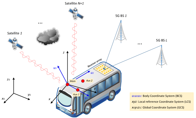
Figure 1: Illustration of a 5G-aided GNSS attitude determination system with $N+1$ GNSS satellites and $L$ 5G BSs. $Main$, $Aux1$, and $Aux2$ are the main and the auxiliary GNSS antennas that define the two baselines, and the BCS is built accordingly. A multi-antenna 5G receiver is equipped to resolve the AoA from different 5G BSs to the receiver array.

2.1 System Description

To take advantage of both GNSS and 5G measurements, a user platform integrating $M+1$ GNSS antennas (which form $M$ baselines) and a multi-antenna 5G receiver is adopted, as shown in Fig. 1. The GNSS observables are the pseudo-range and carrier phase measurements obtained by tracking $N+1$ satellites. These observations are contaminated with errors such as clock biases, instrumental delays, atmospheric delays, and multipath (Teunissen and Montenbruck,, 2017). By double differencing (DD) the pseudo-range and carrier phase observations (i.e. constructing the differences between observations collected at two GNSS antennas from two different satellites), the clock biases, instrumental delays, and atmospheric delays become negligible (Teunissen and Kleusberg,, 2012). The 5G receiver, on the other hand, can receive 5G pilot signals from $L$ BSs (with known positions) and resolve the AoAs of different BSs by applying a channel estimation process (Shahmansoori et al.,, 2018). Hence, we take the estimated AoAs as the 5G observations, whose estimation errors are related to the distance between the specific BS and the receiver, the signal power, the noise level, etc (Zheng et al., 2023a, ). The pilot signals transmitted from different BSs are required to be orthogonal in time and/or frequency to avoid interference between channels.

As depicted in Fig. 1, there are 3 different coordinate systems, namely, body coordinate system (BCS) $u_{1}u_{2}u_{3}$, local reference coordinate system (LCS) $xyz$, and global coordinate system (GCS) $x_{G}y_{G}z_{G}$. The receiver’s BCS is built as follows: the first axis $u_{1}$ is aligned with the first baseline ($Main-Aux1$), the second axis $u_{2}$ is perpendicular to the first, lying in the plane formed by the first two baselines, and the third body axis $u_{3}$ is directed so that $u_{1}u_{2}u_{3}$ forms a right-handed orthogonal frame. In addition, the LCS $xyz$ is defined as keeping the same attitude but a different origin as the GCS (the origins of the LCS and the BCS coincide). The attitude of the user is represented by a rotation matrix ${\bf R}\in\mathrm{SO(3)}$, where $\mathrm{SO(3)}$ denotes the special orthogonal group of 3D rotation matrices as $\mathrm{SO}(3)=\{{\bf R}|{\bf R}^{\mathsf{T}}{\bf R}=\mathbf{I}_{3},\det({\bf R})=1\}.$ The rotation matrix transforms a vector/matrix from the BCS to the LCS. Suppose ${\bf t}^{{\rm B}}$ and ${\bf t}^{{\rm L}}$ represent the coordinates of the same vector expressed in the BCS and the LCS respectively, then they are related through the rotation matrix ${\bf R}$ as

$${\bf t}^{\rm L}={\bf R}{\bf t}^{\rm B}.$$ (1)

2.2 Observation Model

2.2.1 GNSS Observations

Considering a set of $2N$ DD pseudo-range and carrier phase observations obtained at two GNSS antennas (i.e., a single baseline) via tracking the signals from $N+1$ satellites, the functional model is given by

$${\bf y}={\bf A}{\bf z}+{\bf G}{\bf b}+\bm{\epsilon},\quad{\bf Q}({\bf y})=\hbox{\boldmath$\Sigma$}_{\bm{\epsilon}},$$ (2)

where ${\bf y}\in\mathbb{R}^{2N}$ is the vector of DD pseudo-range and carrier phase observations, ${\bf z}\in\mathbb{Z}^{N}$ is the vector of $N$ integer ambiguities, ${\bf b}\in\mathbb{R}^{3}$ denotes the three baseline coordinates (expressed in GCS), and $\bm{\epsilon}\in\mathbb{R}^{2N}$ describes the unmodeled errors. Here, ${\bf A}\in\mathbb{R}^{2N\times N}$ is the design matrix that contains the carrier wavelengths, while ${\bf G}\in\mathbb{R}^{2N\times 3}$ is the matrix formed by the combination of unit line-of-sight vectors. Furthermore, we assume $\bm{\epsilon}$ is an additive white Gaussian noise (AWGN) with zero mean and covariance matrix $\hbox{\boldmath$\Sigma$}_{\bm{\epsilon}}$. Hence, the dispersion on ${\bf y}$, denoted as ${\bf Q}({\bf y})$, is characterized by the covariance matrix $\hbox{\boldmath$\Sigma$}_{\bm{\epsilon}}$.

Since we consider a configuration with multiple GNSS antennas, the observations from different baselines are collected to determine the attitude of the user. For $M+1$ GNSS antennas tracking the same $N+1$ satellites simultaneously, the concatenated observation equation can be formulated as

$${\bf Y}={\bf A}{\bf Z}+{\bf G}{\bf B}+\hbox{\boldmath$\Xi$}_{1},\quad{\bf Q}(\mathrm{vec}({\bf Y}))={\bf P}_{M}\otimes\hbox{\boldmath$\Sigma$}_{\bm{\epsilon}},$$ (3)

where each column of ${\bf Y}\in\mathbb{R}^{2N\times M}$, ${\bf Z}\in\mathbb{Z}^{N\times M}$, and ${\bf B}\in\mathbb{R}^{3\times M}$ contains the pseudo-range and carrier phase observations, the integer ambiguities, and the baseline coordinates for each of the baselines, respectively. The notation $\mathrm{vec}(\cdot)$ stands for the operation of vectorizing a matrix into a vector. Assuming the observations from different baselines keep the same covariance matrix $\hbox{\boldmath$\Sigma$}_{\bm{\epsilon}}$, the covariance matrix of whole observables can be formulated as ${\bf Q}(\mathrm{vec}({\bf Y}))={\bf P}_{M}\otimes\hbox{\boldmath$\Sigma$}_{\bm{\epsilon}}$, where $\otimes$ indicates the Kronecker product and ${\bf P}_{M}\in\mathbb{R}^{M\times M}$ is given by (Teunissen and Kleusberg,, 2012)

$${\bf P}_{M}=\begin{bmatrix}1&0.5&\cdots&0.5\\ 0.5&1&\cdots&0.5\\ \vdots&\vdots&\ddots&\vdots\\ 0.5&0.5&\cdots&1\end{bmatrix}.$$ (4)

Based on (3), the attitude of the user can be connected to observables ${\bf Y}$ through the rotation transformation ${\bf B}={\bf R}{\bf F}$, where ${\bf F}\in\mathbb{R}^{3\times M}$ indicates the baseline coordinates expressed in the BCS. ${\bf F}$ is assumed to be known since we can precisely measure it in advance. Therefore, we can rewrite (3) as

$${\bf Y}={\bf A}{\bf Z}+{\bf G}{\bf R}{\bf F}+\hbox{\boldmath$\Xi$}_{1},\quad{\bf Q}(\mathrm{vec}({\bf Y}))={\bf P}_{M}\otimes\hbox{\boldmath$\Sigma$}_{\bm{\epsilon}}.$$ (5)

For notational convenience, we use ${\bf Q}_{\bf y}$ and ${\bf Q}_{\bf Y}$ to denote ${\bf Q}({\bf y})$ and ${\bf Q}(\mathrm{vec}({\bf Y}))$, respectively.

2.2.2 5G Observations

Consider a down-link scenario for the 5G transmissions. We assume all $L$ 5G BSs work in time-division multiple access (TDMA) mode, where $T$ transmissions of pilot signals are managed by each 5G BS. On the user side, the 5G receiver is an $J_{1}\times J_{2}$ planar antenna array. Thus the received 5G signals at the user platform for the $t$-th transmission from the $\ell$-th BS can be expressed as (Chen et al.,, 2022)

$${\bf y}_{\ell,t}={\bf h}_{\ell}x_{\ell,t}+{\bf n}\in\mathbb{C}^{J_{1}J_{2}\times 1},$$ (6)

where ${\bf h}_{\ell}\in\mathbb{C}^{J_{1}J_{2}\times 1}$ is the channel vector, $x_{\ell,t}$ is the transmitted symbol with a power constraint $|x_{\ell,t}|^{2}=P_{\mathrm{T}}$, and ${\bf n}\sim\mathcal{CN}(\mathbf{0},\sigma^{2}\mathbf{I}_{J_{1}J_{2}})$ denotes the thermal noise at the receiver. Utilizing the far-field model, the $i$-th entry of the channel vector ${\bf h}_{\ell}$ is given by  (Chen et al.,, 2022)

$$h_{\ell,i}=\alpha_{\ell}e^{-j\frac{2\pi f}{c}{\bf p}_{{\rm R},i}^{\mathsf{T}}{\bf t}_{\ell}},$$ (7)

where $\alpha_{\ell}$ denotes the complex gain of the channel between the $\ell$-th BS and the receiver, ${\bf p}_{{\rm R},i}\in\mathbb{R}^{3}$ denotes the position of the $i$-th element of the antenna array at the receiver, and ${\bf t}_{\ell}\in\mathbb{R}^{3}$ represents the direction unit vector that coincides with the AoA of the signal from the $\ell$-th BS to the 5G receiver on the user platform. Note that both ${\bf p}_{{\rm R},i}$ and ${\bf t}_{\ell}$ are expressed in the BCS. Besides, $f$ represents the 5G carrier frequency, $c$ is the speed of light, and $(\cdot)^{\mathsf{T}}$ denotes the transpose operation.

Based on the received symbols ${\bf y}_{\ell,t}$, the AoA vector ${\bf t}_{\ell}$ in the BCS can be estimated via various channel estimators, such as atomic norm minimization (He et al.,, 2021) and ESPRIT (Zheng et al., 2023a, ). Therefore, we define the 5G observables as

$${\bf D}=[{\bf t}_{1},\dots,{\bf t}_{L}]\in\mathbb{R}^{3\times L}.$$ (8)

The dispersion on $\mathrm{vec}({\bf D})$ can be approximated by the inverse of its Fisher information matrix (FIM) (Kay,, 1993; Shahmansoori et al.,, 2018), which we denote as ${\bf Q}_{\bf D}$.

In this work, we assume the position of the user platform ${\bf p}_{\rm U}\in\mathbb{R}^{3}$, which coincides with the origin of the LCS (and the BCS), to be known in the GCS. We further assume the positions of the 5G BSs in the GCS denoted as ${\bf p}_{{\rm B},\ell},\ \ell=1,\dots,L$ to be precisely known. Since we know the positions of the 5G BSs and the user platform, we can compute the columns of ${\bf D}$ expressed in the GCS as

$${\bf t}_{\ell}^{\rm G}=\frac{{\bf p}_{{\rm B},\ell}-{{\bf p}}_{\rm U}}{\|{\bf p}_{{\rm B},\ell}-{{\bf p}}_{\rm U}\|},\quad\ell=1,\dots,L.$$ (9)

Again, the LCS and the GCS have the same attitude but only the origins are different, so ${\bf t}_{\ell}^{\rm L}={\bf t}_{\ell}^{\rm G}$. We further define ${\bf E}=[{\bf t}_{1}^{\rm L},\dots,{\bf t}_{L}^{\rm L}]=[{\bf t}_{1}^{\rm G},\dots,{\bf t}_{L}^{\rm G}]\in\mathbb{R}^{3\times L}$ as the LCS version of ${\bf D}$. Then, according to (1), the 5G observations are related to the user attitude as

$${\bf D}={\bf R}^{\mathsf{T}}{\bf E}+\hbox{\boldmath$\Xi$}_{2},\quad{\bf Q}(\mathrm{vec}({\bf D}))={\bf Q}_{\bf D},$$ (10)

where $\hbox{\boldmath$\Xi$}_{2}\in\mathbb{R}^{3\times L}$ combines additive errors.

2.2.3 Hybrid GNSS-5G Observations

Combining (5) and (10), we have the hybrid observation model for attitude determination as

$$\begin{bmatrix}\mathrm{vec}({\bf Y})\\ \mathrm{vec}({\bf D}^{\mathsf{T}})\end{bmatrix}=\begin{bmatrix}\mathbf{I}\otimes{\bf A}&{\bf F}^{\mathsf{T}}\otimes{\bf G}\\ \mathbf{0}&\mathbf{I}\otimes{\bf E}^{\mathsf{T}}\end{bmatrix}\begin{bmatrix}\mathrm{vec}({\bf Z})\\ \mathrm{vec}({\bf R})\end{bmatrix},$$ (11)

$$\ {\bf Z}\in\mathbb{Z}^{N\times M},\quad{\bf R}\in\mathrm{SO(3)}.$$

Since the GNSS receiver and the 5G receiver are independent, the covariance matrix of the hybrid observables is given by

$${\bf Q}_{{\bf Y},{\bf D}}={\bf Q}([\mathrm{vec}({\bf Y})^{\mathsf{T}},\mathrm{vec}({\bf D}^{\mathsf{T}})^{\mathsf{T}}]^{\mathsf{T}})=\mathrm{blkdiag}({\bf Q}_{\bf Y},{\bf Q}_{\bf D}),$$ (12)

where $\mathrm{blkdiag}(\cdot,\cdot)$ represents constructing a block diagonal matrix from input sub-matrices.

3 ATTITUDE DETERMINATION METHODOLOGY

Based on (11) and (12), the objective function of the hybrid attitude determination problem can be formulated as

$$\min_{{\bf Z}\in\mathbb{Z}^{N\times M},\ {\bf R}\in\mathrm{SO(3)}}\left\|\begin{bmatrix}\mathrm{vec}({\bf Y})\\ \mathrm{vec}({\bf D}^{\mathsf{T}})\end{bmatrix}-\begin{bmatrix}\mathbf{I}\otimes{\bf A}&{\bf F}^{\mathsf{T}}\otimes{\bf G}\\ \mathbf{0}&\mathbf{I}\otimes{\bf E}^{\mathsf{T}}\end{bmatrix}\begin{bmatrix}\mathrm{vec}({\bf Z})\\ \mathrm{vec}({\bf R})\end{bmatrix}\right\|_{{\bf Q}_{{\bf Y},{\bf D}}^{-1}}^{2},$$ (13)

where $\|\cdot\|_{\bf Q}=(\cdot)^{\mathsf{T}}{\bf Q}^{-1}(\cdot)$. The optimization in (13) is a constrained weighted least-squares (LS) problem. Due to the presence of the integer constraints, there exists no closed-form solution for (13). We can first disregard the integer and orthonormality constraints to calculate a closed-form solution for (13), i.e.,a float solution, and then pursue the final constrained solution using a search procedure around the float solution. In the search process, the ambiguities can be resolved based on the integer least-squares (ILS) principle (Teunissen and Tiberius,, 1994). Then, the estimated ambiguities are used to compute the fixed solution.

3.1 The Float Estimator

Without the integer and the orthonormality constraints, based on the LS principle, the normal equations of (13) are given by

$${\bf N}\begin{bmatrix}\mathrm{vec}(\hat{{\bf Z}})\\ \mathrm{vec}(\hat{{\bf R}})\end{bmatrix}=\begin{bmatrix}\mathbf{I}\otimes{\bf A}^{\mathsf{T}}&\mathbf{0}\\ {\bf F}\otimes{\bf G}^{\mathsf{T}}&\mathbf{I}\otimes{\bf E}\end{bmatrix}{\bf Q}_{{\bf Y},{\bf D}}^{-1}\begin{bmatrix}\mathrm{vec}({\bf Y})\\ \mathrm{vec}({\bf D}^{\mathsf{T}})\end{bmatrix},$$ (14)

$${\bf N}=\begin{bmatrix}\mathbf{I}\otimes{\bf A}^{\mathsf{T}}&\mathbf{0}\\ {\bf F}\otimes{\bf G}^{\mathsf{T}}&\mathbf{I}\otimes{\bf E}\end{bmatrix}{\bf Q}_{{\bf Y},{\bf D}}^{-1}\begin{bmatrix}\mathbf{I}\otimes{\bf A}&{\bf F}^{\mathsf{T}}\otimes{\bf G}\\ \mathbf{0}&\mathbf{I}\otimes{\bf E}^{\mathsf{T}}\end{bmatrix}.$$ (15)

That results in the following float solution:

$$\begin{bmatrix}\mathrm{vec}(\hat{{\bf Z}})\\ \mathrm{vec}(\hat{{\bf R}})\end{bmatrix}={\bf N}^{-1}\begin{bmatrix}\mathbf{I}\otimes{\bf A}^{\mathsf{T}}&\mathbf{0}\\ {\bf F}\otimes{\bf G}^{\mathsf{T}}&\mathbf{I}\otimes{\bf E}\end{bmatrix}{\bf Q}_{{\bf Y},{\bf D}}^{-1}\begin{bmatrix}\mathrm{vec}({\bf Y})\\ \mathrm{vec}({\bf D}^{\mathsf{T}})\end{bmatrix}.$$ (16)

The covariance matrix of this float solution is obtained by inversion of the normal matrix, i.e.,

$${\bf Q}_{\mathrm{hybrid}}=\begin{bmatrix}{\bf Q}_{\hat{{\bf Z}}}&{\bf Q}_{\hat{{\bf Z}}\hat{{\bf R}}}\\ {\bf Q}_{\hat{{\bf R}}\hat{{\bf Z}}}&{\bf Q}_{\hat{{\bf R}}}\end{bmatrix}={\bf N}^{-1}.$$ (17)

Now, we can show the superiority of the hybrid solution in (16) by analyzing the covariance matrix ${\bf Q}_{\mathrm{hybrid}}$. Defining ${\bf M}_{1}=[\mathbf{I}\otimes{\bf A},\ {\bf F}^{\mathsf{T}}\otimes{\bf G}]$ and ${\bf M}_{2}=[\mathbf{0},\ \mathbf{I}\otimes{\bf E}^{\mathsf{T}}]$, we have

$${\bf Q}_{\mathrm{hybrid}}^{-1}=\begin{bmatrix}{\bf M}_{1}^{\mathsf{T}}&{\bf M}_{2}^{\mathsf{T}}\end{bmatrix}\begin{bmatrix}{\bf Q}_{\bf Y}^{-1}&\mathbf{0}\\ \mathbf{0}&{\bf Q}_{\bf D}^{-1}\end{bmatrix}\begin{bmatrix}{\bf M}_{1}\\ {\bf M}_{2}\end{bmatrix}=\underbrace{{\bf M}_{1}^{\mathsf{T}}{\bf Q}_{\bf Y}^{-1}{\bf M}_{1}}_{{\bf Q}_{\mathrm{GNSS}}^{-1}}+\underbrace{{\bf M}_{2}^{\mathsf{T}}{\bf Q}_{\bf D}^{-1}{\bf M}_{2}}_{{\bf Q}_{\mathrm{5G}}^{-1}},$$ (18)

where ${\bf Q}_{\mathrm{GNSS}}$ and ${\bf Q}_{\mathrm{5G}}$ represent the covariance matrices of the standalone GNSS and 5G float solutions, respectively. Since the covariance matrices ${\bf Q}_{\mathrm{hybrid}}$, ${\bf Q}_{\mathrm{GNSS}}$, and ${\bf Q}_{\mathrm{5G}}$ are positive semidefinite, we have

$${\bf Q}_{\mathrm{hybrid}}^{-1}\succeq{\bf Q}_{\mathrm{GNSS}}^{-1},\qquad{\bf Q}_{\mathrm{hybrid}}^{-1}\succeq{\bf Q}_{\mathrm{5G}}^{-1},$$ (19)

where ${\bf A}\succeq{\bf B}$ stands for matrix ${\bf A}-{\bf B}$ is positive semidefinite. The relationships in (19) immediately yield (Horn and Johnson,, 2012)

$${\bf Q}_{\mathrm{hybrid}}\preceq{\bf Q}_{\mathrm{GNSS}},\qquad{\bf Q}_{\mathrm{hybrid}}\preceq{\bf Q}_{\mathrm{5G}}.$$ (20)

Hence we have

$$\mathrm{Tr}({\bf Q}_{\mathrm{hybrid}})\leq\mathrm{Tr}({\bf Q}_{\mathrm{GNSS}}),\qquad\mathrm{Tr}({\bf Q}_{\mathrm{hybrid}})\leq\mathrm{Tr}({\bf Q}_{\mathrm{5G}}),$$ (21)

where $\mathrm{Tr}(\cdot)$ returns the trace of a square matrix. Here, (21) stipulates that the error covariance of the hybrid solution (16) is lower than that of either of the standalone GNSS/5G solutions.

3.2 The Multivariate Constrained Estimator

Following a similar procedure to the standard method for GNSS attitude determination (Giorgi and Teunissen,, 2010), the objective function can be decomposed based on the float solution in (16) as follows:

$$\min_{{\bf Z}\in\mathbb{Z}^{N\times M},\ {\bf R}\in\mathrm{SO(3)}} \left\|\begin{bmatrix}\mathrm{vec}({\bf Y})\\ \mathrm{vec}({\bf D}^{\mathsf{T}})\end{bmatrix}-\begin{bmatrix}\mathbf{I}\otimes{\bf A}&{\bf F}^{\mathsf{T}}\otimes{\bf G}\\ \mathbf{0}&\mathbf{I}\otimes{\bf E}^{\mathsf{T}}\end{bmatrix}\begin{bmatrix}\mathrm{vec}({\bf Z})\\ \mathrm{vec}({\bf R})\end{bmatrix}\right\|_{{\bf Q}_{{\bf Y},{\bf D}}^{-1}}^{2}$$ (22)

$$= \left\|\begin{bmatrix}\mathrm{vec}({\bf Y})\\ \mathrm{vec}({\bf D}^{\mathsf{T}})\end{bmatrix}-\begin{bmatrix}\mathbf{I}\otimes{\bf A}&{\bf F}^{\mathsf{T}}\otimes{\bf G}\\ \mathbf{0}&\mathbf{I}\otimes{\bf E}^{\mathsf{T}}\end{bmatrix}\begin{bmatrix}\mathrm{vec}(\hat{\bf Z})\\ \mathrm{vec}(\hat{\bf R})\end{bmatrix}\right\|_{{\bf Q}_{{\bf Y},{\bf D}}^{-1}}^{2}$$

$$\qquad+\mathop{\min}\limits_{{\bf Z}\in\mathbb{Z}^{N\times M}}\left(\left\|{\mathrm{vec}\!\left({\bf Z}-\hat{\bf Z}\right)}\right\|_{{\bf Q}_{\hat{{\bf Z}}}^{-1}}^{2}+\mathop{\min}\limits_{{\bf R}\in\mathrm{SO(3)}}\left\|{\mathrm{vec}\left({\bf R}-\hat{\bf R}\left({\bf Z}\right)\right)}\right\|_{{\bf Q}_{{\hat{{\bf R}}}\left({\bf Z}\right)}^{-1}}^{2}\right).$$

If the integer ambiguities ${\bf Z}$ are known, the float estimate of ${\bf R}$ can be updated as (Giorgi and Teunissen,, 2010)

$$\mathrm{vec}(\hat{{\bf R}}({\bf Z}))=\mathrm{vec}(\hat{{\bf R}})-{\bf Q}_{\hat{{\bf R}}\hat{{\bf Z}}}{\bf Q}_{\hat{{\bf Z}}}^{-1}\mathrm{vec}(\hat{{\bf Z}}-{\bf Z}).$$ (23)

The covariance matrix of the updated solution is given by

$${\bf Q}_{\hat{{\bf R}}({\bf Z})}={\bf Q}_{\hat{{\bf R}}}-{\bf Q}_{\hat{{\bf R}}\hat{{\bf Z}}}{\bf Q}_{\hat{{\bf Z}}}^{-1}{\bf Q}_{\hat{{\bf Z}}\hat{{\bf R}}}.$$ (24)

Note that the first term of the right-hand side of (22) does not depend on $\mathbf{Z}$ and $\mathbf{R}$. Consequently, the integer ambiguities can be resolved based on the following minimization problem:

$$\check{\bf Z}=\mathop{\arg\min}\limits_{{\bf Z}\in\mathbb{Z}^{N\times M}}\mathcal{C}\!\left({\bf Z}\right),$$ (25)

where

$$\mathcal{C}\!\left({\bf Z}\right)=\left\|{\mathrm{vec}\!\left({\bf Z}-\hat{\bf Z}\right)}\right\|_{{\bf Q}_{\hat{{\bf Z}}}^{-1}}^{2}+\mathop{\min}\limits_{{\bf R}\in\mathrm{SO(3)}}\left\|{\mathrm{vec}\left({\bf R}-\hat{\bf R}\left({\bf Z}\right)\right)}\right\|_{{\bf Q}_{{\hat{{\bf R}}}\left({\bf Z}\right)}^{-1}}^{2},$$ (26)

while the fixed solution of the rotation matrix is given by

$$\check{\bf R}=\mathop{\min}\limits_{{\bf R}\in\mathrm{SO(3)}}\left\|{\mathrm{vec}\left({\bf R}-\hat{\bf R}\left(\check{\bf Z}\right)\right)}\right\|_{{\bf Q}_{{\hat{{\bf R}}}\left({\bf Z}\right)}^{-1}}^{2}.$$ (27)

An efficient integer search strategy, either the search-and-shrink or search-and-expansion algorithm, can be utilized to solve (25) (Giorgi and Teunissen,, 2010).

4 Performance Evaluation

4.1 Evaluation Setup

Table 1: The relative positions of the 5G BSs (m)

	BS 1	BS 2	BS 3	BS 4	BS 5	BS 6	BS 7	BS 8
$x$	10	-10	5	-5	15	-15	0	0
$y$	10	-10	10	-10	0	0	15	-15
$z$	10	10	15	15	10	10	10	10

The simulations are implemented using the real data of satellite orbit information and the assumed user position and attitude. We generate GNSS observations based on only GPS constellation. Without further specification, the default number of the tracked GPS satellites that we simulate is 5. We use 4 GNSS antennas which form 3 baselines with unit vectors ${\bf b}_{1}=[1,0,0]^{\mathsf{T}}$, ${\bf b}_{2}=[0,1,0]^{\mathsf{T}}$, and ${\bf b}_{3}=[0,0,1]^{\mathsf{T}}$, in units of meters. We set the standard deviation of the carrier-phase measurements equal to a value $\sigma$ and that of the pseudo-range data equal to $100\sigma$. By default, we set $\sigma=0.001\,\mathrm{m}$. The position of the $i$-th 5G BSs is denoted as ${\bf p}_{i}={\bf p}_{\rm U}+\Delta{\bf p}_{i}$. For trials under different number of 5G BSs, the BS’s relative positions to the user platform, $\Delta{\bf p}_{i},\ i=1,...,8,$ are picked from Table 1. The 5G BSs transmit pilots at a carrier frequency of $28\,\mathrm{GHz}$ with $300\,\mathrm{MHz}$ bandwidth, and the size of the receiver array is set as $5\times 5$ with half-wavelength spacing. By default, we set the number of 5G transmissions at a single observation as $T=128$, and the average transmission power is $17\,\mathrm{dBm}$. We assume the received 5G signals are contaminated by an AWGN with a noise power spectral density of $-174\,\mathrm{dBm/Hz}$. Therefore, the covariance matrix of the 5G observations ${\bf D}$ in (8) can be evaluated by the inverse of the FIM, as specified in (Zheng et al.,, 2022; Zheng et al., 2023a, ).

Throughout the simulation studies, the proposed method is compared with the standalone GNSS and the standalone 5G methods, which use the pure GNSS and the pure 5G observations, respectively. For standalone GNSS estimation, we use the method proposed in (Giorgi and Teunissen,, 2010). For standalone 5G estimation, we use the method proposed in (Zheng et al.,, 2022, Sec. V-C).

4.2 Simulation Results

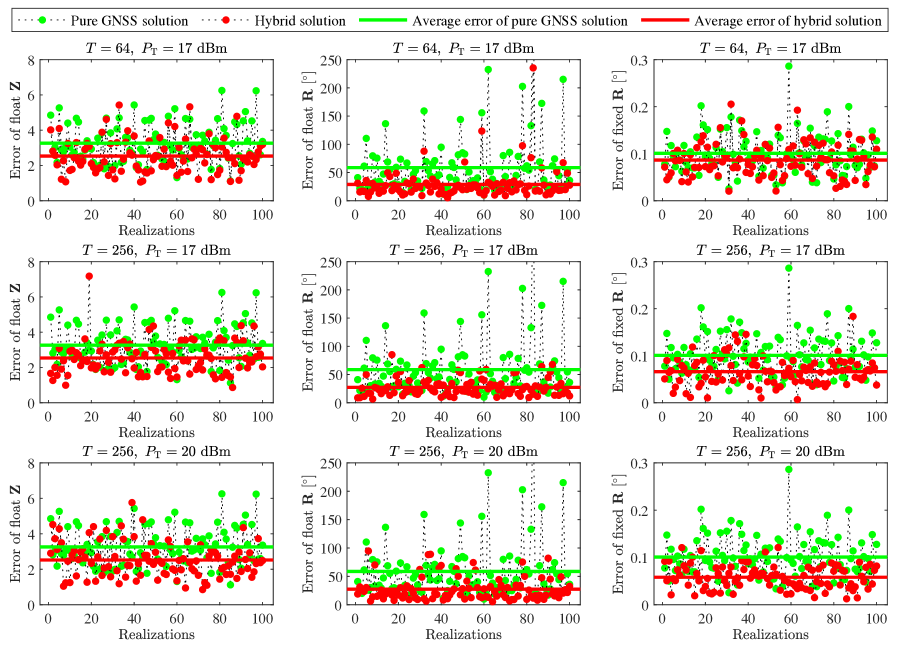
Figure 2: Estimation errors of the float ambiguity ${\bf Z}$, the float attitude ${\bf R}$, and the fixed attitude ${\bf R}$ for the pure GNSS solution and the hybrid solution (aided by a single 5G BS) under setups: (i) $T=64,\ P_{\mathrm{T}}=17\,\mathrm{dBm}$; (ii) $T=256,\ P_{\mathrm{T}}=17\,\mathrm{dBm}$; (iii) $T=256,\ P_{\mathrm{T}}=20\,\mathrm{dBm}$.

We first consider a scenario with a single 5G BS to aid GNSS attitude determination. In this case, a standalone 5G attitude estimation is impossible. Note that the performance of the 5G-based estimation usually depends on the transmission number $T$ and the signal power $P_{\mathrm{T}}$, whose impact will be tested in our simulations. Fig. 2 shows the estimation errors of the float ambiguity ${\bf Z}$, the float attitude ${\bf R}$, and the fixed attitude ${\bf R}$ for the pure GNSS solution and the hybrid solution, under 3 different setups of the 5G transmissions $T$ and signal power $P_{\mathrm{T}}$, i.e.: (i) $T=64,\ P_{\mathrm{T}}=17\,\mathrm{dBm}$; (ii) $T=256,\ P_{\mathrm{T}}=17\,\mathrm{dBm}$; (iii) $T=256,\ P_{\mathrm{T}}=20\,\mathrm{dBm}$. The presented errors are calculated as the Frobenius norm of the difference between the estimated unknown matrices and the true ones. We plot the average errors computed from 100 independent realizations for each setup, and the corresponding average errors are computed and plotted. It can be clearly seen that even a single 5G BS can help reduce the estimation errors of the GNSS attitude determination, in both the float solution and the fixed solution. In addition, the estimation performance can be effectively improved by increasing the 5G transmissions $T$ and the 5G signal power $P_{\mathrm{T}}$.

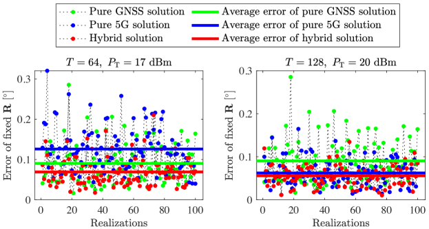
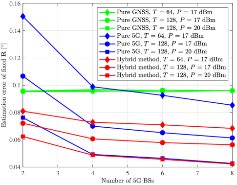
Figure 3: Estimation errors of the fixed attitude solution (of ${\bf R}$) for the pure GNSS solution, the pure 5G solution with 3 BSs, and the hybrid solution (aided by 3 5G BSs) in 2 different setups: (i) $T=64,\ P_{\mathrm{T}}=17\,\mathrm{dBm}$; (ii) $T=128,\ P_{\mathrm{T}}=20\,\mathrm{dBm}$.

Figure 4: The average estimation errors of the pure GNSS solution, the pure 5G solution, and the hybrid solution versus the number of 5G BSs.

Next, we test the estimation performance when the number of 5G BSs is increased to 3. In these cases, a standalone 5G attitude determination is feasible. Therefore, we assess and compare the performance of the pure GNSS solution, the pure 5G solution, and the hybrid solution, to demonstrate the superiority of the proposed hybrid solution. Fig. 4 demonstrates the estimation errors of the fixed attitude ${\bf R}$ for the pure GNSS solution, the pure 5G solution, and the hybrid solution under 2 different setups: (i) $T=64,\ P_{\mathrm{T}}=17\,\mathrm{dBm}$; (ii) $T=128,\ P_{\mathrm{T}}=20\,\mathrm{dBm}$. For each setup, the results from 100 independent realizations are presented along with the average errors. We can observe that the hybrid solution outperforms the two standalone methods under various setups (when the pure GNSS solution outperforms the pure 5G solution or vice versa), which reveals that despite the feasibility of the pure GNSS and 5G solutions, the hybrid method can provide a further performance improvement.

Table 2: Success Rate of the Ambiguity Resolution ($\sigma~{}=~{}0.03\,\mathrm{m},\ T=64$)

	0	1	2	3	4
5	0%	0%	0%	14%	60%
6	0%	0%	0%	26%	63%
7	0%	0%	0%	27%	67%
8	0%	0%	0%	30%	68%

Table 3: Estimation Error of the Fixed Attitude (^∘) ($\sigma~{}=~{}0.03\,\mathrm{m},\ T=64$)

	0	1	2	3	4
5	95.41	80.99	12.81	0.38	0.10
6	92.26	81.37	12.85	0.31	0.09
7	90.76	79.25	9.35	0.26	0.09
8	87.70	79.13	9.31	0.19	0.09

Table 4: Success Rate of the Ambiguity Resolution ($\sigma~{}=~{}0.03\,\mathrm{m},\ T=512$)

	0	1	2	3	4
5	0%	0%	0%	16%	70%
6	0%	0%	0%	21%	71%
7	0%	0%	0%	28%	75%
8	0%	0%	0%	32%	75%

Table 5: Estimation Error of the Fixed Attitude (^∘) ($\sigma~{}=~{}0.03\,\mathrm{m},\ T=512$)

	0	1	2	3	4
5	93.09	80.69	12.69	0.08	0.04
6	86.54	80.31	6.84	0.06	0.03
7	87.90	80.28	7.52	0.06	0.03
8	85.02	81.12	2.44	0.06	0.03

Table 6: Success Rate of the Ambiguity Resolution ($\sigma~{}=~{}0.003\,\mathrm{m},\ T=512$)

	0	1	2	3	4
5	14%	100%	100%	100%	100%
6	98%	100%	100%	100%	100%
7	100%	100%	100%	100%	100%
8	100%	100%	100%	100%	100%

Table 7: Estimation Error of the Fixed Attitude (^∘) ($\sigma~{}=~{}0.003\,\mathrm{m},\ T=512$)

	0	1	2	3	4
5	30.00	0.11	0.06	0.06	0.03
6	1.33	0.11	0.06	0.05	0.03
7	0.21	0.10	0.06	0.05	0.02
8	0.22	0.09	0.06	0.04	0.02

In Fig. 4, we further evaluate the root mean square errors (RMSEs) of the pure GNSS solution, the pure 5G solution, and the hybrid solution, for different numbers of 5G BSs $L=\{2,4,6,8\}$. The RMSE at each point is computed from 10000 independent trials. Three setups are tested, i.e.: (i) $T=64,\ P_{\mathrm{T}}=17\,\mathrm{dBm}$; (ii) $T=128,\ P_{\mathrm{T}}=17\,\mathrm{dBm}$; (iii) $T=128,\ P_{\mathrm{T}}=20\,\mathrm{dBm}$. We can see that the performance of both the pure 5G solution and the hybrid solution improve as the number of 5G BSs increases, while the performance of the pure GNSS solution remains unchanged. In all the tested cases, the hybrid solution outperforms the other two methods. However, we observe that the gap between the errors of the pure 5G solution and the hybrid solution decreases with any increase in the number of 5G BSs $L$, the number of the 5G transmissions $T$, or the 5G signal power $P_{\mathrm{T}}$. This phenomenon indicates a performance saturation of the hybrid solution. Specifically, we can conclude that: (i) By increasing the number of 5G BSs $L$, the number of the 5G transmissions $T$, and/or the 5G transmission power $P_{\mathrm{T}}$, the performance of the pure 5G solution can be improved; (ii) the hybrid method cannot provide a significant performance improvement when the pure 5G solution is already much more accurate than the pure GNSS solution. However, in practical situations, maintaining 5G connection between the user platform and a large number of 5G BSs (with large power and transmission allocation) may not be achievable, where our proposed method can provide a significant performance improvement.

Finally, Table 7–Table 7 demonstrate the success rate of the ambiguity resolution and the average estimation error of the fixed attitude of the proposed hybrid method for different numbers of satellites and different numbers of 5G BSs. Note that the case where $L=0$ coincides with the pure GNSS solution. In these trials, 3 setups are tested: (i) $\sigma~{}=~{}0.03\,\mathrm{m},\ T=64$; (ii) $\sigma~{}=~{}0.03\,\mathrm{m},\ T=512$; (iii) $\sigma~{}=~{}0.003\,\mathrm{m},\ T=512$. First, for high carrier-phase standard deviations $\sigma$ (e.g., $\sigma=0.03$), the standalone GNSS method cannot resolve the integer ambiguity at all with all the tested number of satellites. However, when there are enough 5G BSs involved (e.g., $L=\{3,4\}$), the success rate becomes greater than zero, and the more 5G BSs we utilize, the higher the ambiguity resolution success rate. Consequently, it is naturally observed that the average estimation error is lowered with the increment of the ambiguity resolution success rate. By comparing Table 7 and Table 7, we observe that increasing the number of 5G transmissions also helps lower estimation errors. Furthermore, the results in Table 7 and Table 7 show that even with successfully resolved integer ambiguities, increasing the number of 5G BSs and the number of satellites is helpful in enhancing the attitude estimation accuracy.

5 Conclusion

This paper formulated and solved the hybrid 5G-GNSS attitude determination problem, which is a promising solution in deep urban areas. The observation model of the GNSS and 5G systems are described, where the hybrid observables consist of the GNSS pseudo-ranges, GNSS carrier phases, and 5G AoAs. By rigorously incorporating these observations, a constrained weighted LS problem is constructed. This problem is solved by first obtaining an unconstrained float solution, then applying the MC-LAMBDA procedure to resolve integer ambiguity and obtain the fixed solution. The proposed hybrid solution is compared with the pure GNSS and the pure 5G solutions, which showed the superiority of the proposed hybrid solution in both enhancing the ambiguity resolution success rate and improving the estimation accuracy.

References

- 3GPP, (2023) 3GPP (2023). 3GPP TR 23.700-86 V18.0.0: Study on Architecture Enhancement to support ranging based services and sidelink positioning (Release 18).
- Abu-Shaban et al., (2018) Abu-Shaban, Z., Zhou, X., Abhayapala, T., Seco-Granados, G., and Wymeersch, H. (2018). Error bounds for uplink and downlink 3D localization in 5G millimeter wave systems. IEEE Transactions on Wireless Communications, 17(8):4939–4954.
- Alletto et al., (2016) Alletto, S., Cucchiara, R., Del Fiore, G., Mainetti, L., Mighali, V., Patrono, L., and Serra, G. (2016). An indoor location-aware system for an IoT-based smart museum. IEEE Internet of Things Journal, 3(2):244–253.
- Angrisano et al., (2010) Angrisano, A. et al. (2010). GNSS/INS integration methods. Dottorato di ricerca (PhD) in Scienze Geodetiche e Topografiche Thesis, Universita’degli Studi di Napoli PARTHENOPE, Naple, 21.
- Chen et al., (2022) Chen, H., Sarieddeen, H., Ballal, T., Wymeersch, H., Alouini, M.-S., and Al-Naffouri, T. Y. (2022). A tutorial on terahertz-band localization for 6G communication systems. IEEE Communications Surveys & Tutorials, 24(3):1780–1815.
- Chen et al., (2023) Chen, H., Zheng, P., Keskin, M. F., Al-Naffouri, T. Y., and Wymeersch, H. (2023). Multi-RIS-enabled 3D sidelink positioning. preprint arXiv:2302.12459.
- del Peral-Rosado et al., (2018) del Peral-Rosado, J. A., Raulefs, R., López-Salcedo, J. A., and Seco-Granados, G. (2018). Survey of cellular mobile radio localization methods: From 1G to 5G. IEEE Communications Surveys & Tutorials, 20(2):1124–1148.
- Di Taranto et al., (2014) Di Taranto, R., Muppirisetty, S., Raulefs, R., Slock, D., Svensson, T., and Wymeersch, H. (2014). Location-aware communications for 5G networks: How location information can improve scalability, latency, and robustness of 5G. IEEE Signal Processing Magazine, 31(6):102–112.
- Douik et al., (2020) Douik, A., Liu, X., Ballal, T., Al-Naffouri, T. Y., and Hassibi, B. (2020). Precise 3-D GNSS attitude determination based on Riemannian manifold optimization algorithms. IEEE Transactions on Signal Processing, 68:284–299.
- Falco et al., (2017) Falco, G., Pini, M., and Marucco, G. (2017). Loose and tight GNSS/INS integrations: Comparison of performance assessed in real urban scenarios. Sensors, 17(2):255.
- Giorgi and Teunissen, (2010) Giorgi, G. and Teunissen, P. J. (2010). Carrier phase GNSS attitude determination with the multivariate constrained LAMBDA method. In IEEE Aerospace Conference.
- Groves, (2013) Groves, P. (2013). GNSS solutions: Multipath vs. NLOS signals. how does non-line-of-sight reception differ from multipath interference. Inside GNSS Magazine, 8(6):40–42.
- He et al., (2021) He, J., Wymeersch, H., and Juntti, M. (2021). Channel estimation for RIS-aided mmwave MIMO systems via atomic norm minimization. IEEE Transactions on Wireless Communications, 20(9):5786–5797.
- Horn and Johnson, (2012) Horn, R. A. and Johnson, C. R. (2012). Matrix analysis. Cambridge university press.
- Jiang et al., (2021) Jiang, C., He, Y., Zheng, X., and Liu, Y. (2021). Omnitrack: Orientation-aware RFID tracking with centimeter-level accuracy. IEEE Transactions on Mobile Computing, 20(2):634–646.
- Kay, (1993) Kay, S. M. (1993). Fundamentals of statistical signal processing: estimation theory. Prentice-Hall, Inc.
- Liu, (2023) Liu, X. (2023). GNSS Localization and Attitude Determination via Optimization Techniques on Riemannian Manifolds. PhD thesis.
- (18) Liu, X., Ballal, T., Ahmed, M., and Al-Naffouri, T. Y. (2022a). A GNSS attitude determination algorithm using optimization techniques on Riemannian manifolds. In Proceedings of the 35th International Technical Meeting of the Satellite Division of The Institute of Navigation (ION GNSS+ 2022), pages 2064–2073.
- Liu et al., (2023) Liu, X., Ballal, T., Ahmed, M., and Al-Naffouri, T. Y. (2023). Instantaneous GNSS ambiguity resolution and attitude determination via Riemannian manifold optimization. IEEE Transactions on Aerospace and Electronic Systems, 59(3):3296–3312.
- Liu et al., (2019) Liu, X., Ballal, T., and Al-Naffouri, T. Y. (2019). GNSS-based localization for autonomous vehicles: Prospects and challenges. In 27th European Signal Processing Conference (EUSIPCO).
- Liu et al., (2020) Liu, X., Ballal, T., and Al-Naffouri, T. Y. (2020). GNSS attitude determination using a constrained wrapped least squares approach. In 2020 IEEE/ION Position, Location and Navigation Symposium (PLANS), pages 1135–1139.
- (22) Liu, X., Ballal, T., Chen, H., and Al-Naffouri, T. Y. (2022b). Constrained wrapped least squares: A tool for high-accuracy GNSS attitude determination. IEEE Transactions on Instrumentation and Measurement, 71:1–15.
- Shahmansoori et al., (2018) Shahmansoori, A., Garcia, G. E., Destino, G., Seco-Granados, G., and Wymeersch, H. (2018). Position and orientation estimation through millimeter-wave MIMO in 5G systems. IEEE Transactions on Wireless Communications, 17(3):1822–1835.
- Teunissen, (2012) Teunissen, P. (2012). The affine constrained GNSS attitude model and its multivariate integer least-squares solution. Journal of geodesy, 86(7):547–563.
- Teunissen and Tiberius, (1994) Teunissen, P. and Tiberius, C. (1994). Integer least-squares estimation of the GPS phase ambiguities. In Proceedings of the International Symp. On Kinematic Systems in Geodesy, Aug, 30-Sept. 2, 1994, Banff, Canada, 11 pp.
- Teunissen and Kleusberg, (2012) Teunissen, P. J. and Kleusberg, A. (2012). GPS for Geodesy. Springer Science & Business Media.
- Teunissen and Montenbruck, (2017) Teunissen, P. J. and Montenbruck, O. (2017). Springer handbook of global navigation satellite systems, volume 10. Springer.
- Wen et al., (2021) Wen, W., Pfeifer, T., Bai, X., and Hsu, L.-T. (2021). Factor graph optimization for GNSS/INS integration: A comparison with the extended Kalman filter. NAVIGATION: Journal of the Institute of Navigation, 68(2):315–331.
- Zheng et al., (2022) Zheng, P., Ballal, T., Chen, H., Wymeersch, H., and Al-Naffouri, T. Y. (2022). Coverage analysis of joint localization and communication in THz systems with 3D arrays. TechRxiv preprint.
- (30) Zheng, P., Chen, H., Ballal, T., Valkama, M., Wymeersch, H., and Al-Naffouri, T. Y. (2023a). JrCUP: Joint RIS calibration and user positioning for 6G wireless systems. preprint arXiv:2304.00631.
- (31) Zheng, P., Chen, H., Ballal, T., Wymeersch, H., and Al-Naffouri, T. Y. (2023b). Misspecified Cramér-Rao bound of RIS-aided localization under geometry mismatch. In 2023 IEEE International Conference on Acoustics, Speech and Signal Processing (ICASSP).
- (32) Zheng, P., Liu, X., Ballal, T., and Al-Naffouri, T. Y. (2023c). 5G-aided RTK positioning in GNSS-deprived environments. In 31th European Signal Processing Conference (EUSIPCO).