Non-perturbative $\langle\phi\rangle$, $\langle\phi^{2}\rangle$ and the dynamically generated scalar mass with Yukawa interaction in the inflationary de Sitter spacetime

Abstract

We consider a massless minimally coupled self interacting quantum scalar field coupled to fermion via the Yukawa interaction, in the inflationary de Sitter background. The fermion is also taken to be massless and the scalar potential is taken to be a hybrid, $V(\phi)=\lambda\phi^{4}/4!+\beta\phi^{3}/3!$ ($\lambda>0$). The chief physical motivation behind this choice of $V(\phi)$ corresponds to, apart from its boundedness from below property, the fact that shape wise $V(\phi)$ has qualitative similarity with standard inflationary classical slow roll potentials. Also, its vacuum expectation value can be negative, suggesting some screening of the inflationary cosmological constant. We choose that $\langle\phi\rangle\sim 0$ at early times with respect to the Bunch-Davies vacuum, so that perturbation theory is valid initially. We consider the equations satisfied by $\langle\phi(t)\rangle$ and $\langle\phi^{2}(t)\rangle$, constructed from the coarse grained equation of motion for the slowly rolling $\phi$. We then compute the vacuum diagrammes of various relevant operators using the in-in formalism up to three loop, in terms of the leading powers of the secular logarithms. For a closed fermion loop, we have restricted ourselves here to only the local contribution. These large temporal logarithms are then resummed by constructing suitable non-perturbative equations to compute $\langle\phi\rangle$ and $\langle\phi^{2}\rangle$. $\langle\phi\rangle$ turns out to be at least approximately an order of magnitude less compared to the minimum of the classical potential, $-3\beta/\lambda$, owing to the strong quantum fluctuations. For $\langle\phi^{2}\rangle$, we have computed the dynamically generated scalar mass at late times, by taking the appropriate purely local contributions. Variations of these quantities with respect to different couplings have also been presented.

Keywords : Massless minimal scalar, self interaction, fermions, de Sitter spacetime, tadpoles, resummation, dynamical mass

1 Introduction

It is well accepted by now that the so called hot big bang cosmological model has been amply successful in explaining the redshifts of galaxies, the origin of the cosmic microwave background radiation, abundance of light elements and the formation of large scale cosmic structures of our universe. However, a few puzzling issues such as the spatial flatness of our universe, the horizon problem and the hitherto unobserved relics such as the magnetic monopoles in terms of their scarcity, cannot be addressed by this model [1, 2, 3, 4]. The paradigm of the primordial cosmic inflation is a conjectured phase of very rapid, near exponential accelerated expansion of our very early universe, introduced to provide possible answers to these aforementioned problems. In other words, the primordial inflation can be thought of as an initial condition to our universe. Indeed, inflation does not only solve these problems, but also provides an elegant mechanism to generate primordial quantum cosmological density perturbations, as a seed to the large scale cosmic structures we observe today in the sky, see [3, 4] and references therein for various theoretical and observational aspects of cosmic inflation.

In order to drive an accelerated expansion of the universe, usually some exotic matter with positive energy density but negative isotropic pressure is needed, known as the dark energy, the simplest form of which is regarded as the positive cosmological constant, $\Lambda$. For the latter in particular, the corresponding spacetime in the absence of any other backreaction is known as the de Sitter spacetime, which has an exponential scale factor and a maximal isometry group. Many computations can be done exactly in this background, owing to its maximal symmetry. The early inflationary phase of our universe was expected to be dominated by dark energy/positive cosmological constant, whose density must had been much larger compared to that of we observe today. It is an important task to understand how the inflationary $\Lambda$ got diminished to reach its current observed tiny value. This question seems to become more intriguing once we recall that only about $10\%$ deviation to the current $\Lambda$-value would have made the universe very different from what we observe it today, e.g. [5]. Since we are essentially talking about a time dependent, expanding spacetime background here, we must not ignore the quantum effects which one may reasonably expect to be large in this context. At least a part of the problem then essentially boils down to estimating the backreaction of quantum fields, to see to what extent these backreactions can screen the inflationary $\Lambda$ or break the de Sitter invariance, at the time of the graceful exit, see [5, 6, 7] and references therein. We also refer our reader to e.g. [8, 9, 10, 11, 12, 13, 14] for alternative proposals to the solution of the aforementioned cosmic coincidence as well as the cosmological constant problem. In any case, analysing matter field’s backreaction in the inflationary background seems to be an important and challenging task.

Massless yet conformally non-invariant matter fields such as a massless minimally coupled scalar or gravitons break the de Sitter invariance and can generate non-perturbative effects monotonically growing with time, popularly regarded as the secular effect, at late cosmological times [15]. These effects correspond to the late time, long wavelength infrared modes. There can be instances in which such infrared contributions can be resummed, to produce finite and physically acceptable answers. The problem of resumming the secular effect for infrared gravitons however, remains as an open challenge, see [7] and references therein. The secular effect for a self interacting massless and minimally coupled scalar field coupled to fermions in the de Sitter spacetime will be the chief concern of this paper.

Quantisation of the massless or massive or conformally invariant scalar fields and their comoving Unruh-DeWitt detector responses in the de Sitter spacetime can be seen in [16, 17, 18, 19, 20, 21, 22, 23]. For a massless and minimally coupled scalar, there exists no de Sitter invariant vacuum state, as was pointed out long ago via the computation of the Wightman functions in [20, 21]. The corresponding de Sitter breaking term is given via the logarithm of the scale factor. Consequently, while doing perturbation theory using these scalar two point functions, each internal line in a given Feynman diagram may yield one such logarithm, growing monotonically with time. Such temporal growth would eventually make the amplitude non-perturbatively large, indicating a possible breakdown of the perturbation theory after sufficient number of $e$-foldings. Such secular effects at one and two loops for self interacting scalar field theories, scalar quantum electrodynamics and even in the context of perturbative quantum gravity were computed in [24, 25, 26, 27, 28, 29, 30, 31, 32, 33, 34, 35, 36, 37] and references therein. Attempts to resum such non-perturbative infrared effects in order to extract finite quantities such as the dynamically generated mass at late times can be seen in e.g., [7, 38, 39, 40, 41, 42, 43, 44, 45, 46, 47, 48, 49, 50, 51, 52, 53, 54] (also references therein). Note that such resummation should not be regarded as physically similar to that of the standard renormalisation group, as the secular effect is essentially a long wavelength infrared phenomenon and the renormalisation counterterms play no role while summing them, e.g. [7].

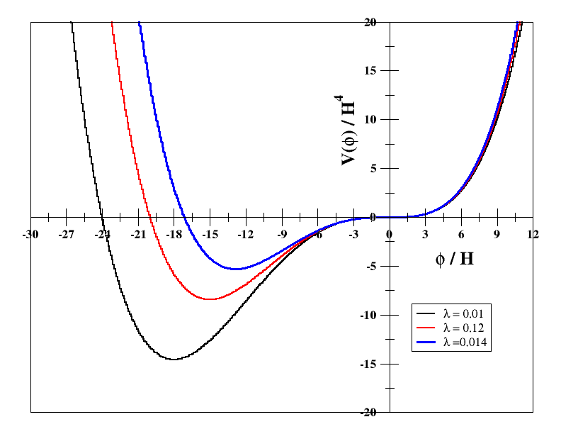
Figure 1: The feature of the self interaction potential for the scalar field, 1, with $\bar{\beta}=\beta/H\sim 0.06$. All relevant quantities are made dimensionless with respect to the de Sitter Hubble constant, $H$. For negative values of $\bar{\beta}$, the minima just gets shifted to the other side of the vertical axis. Although the minima gets deepened with increasing $\bar{\beta}/\lambda$, the potential always remains bounded from below. We also note the shape-wise similarity of this hybrid potential to the standard slow roll (e.g. [4]) ones.

A very efficient and infrared effective method to treat a self interacting scalar field theory non-perturbatively in the inflationary background is the stochastic formalism, proposed in the pioneering works [55, 56]. We further refer our reader to [57, 58, 59, 60, 61, 62, 63, 64, 65] and references therein for recent developments. This method is very efficient for computing expectation values associated with the super-Hubble or infrared part of the scalar field with a potential bounded from below, with respect to some late time equilibrium state. These deep infrared modes receive quantum-kicks from the stochastic forces rendered by the sub-Hubble modes as well as a drag due to the gradient of the potential, similar to that of the Brownian motion. The stochastic formalism basically maps a problem of quantum field theory into a classical statistical one. Putting things together now, all these non-perturbative results strongly suggest that it is the perturbation theory that remains invalid at late times, and proper non-perturbative treatment shows consistency with the de Sitter symmetry, owing to the dynamical mass generation of the scalar. A massive scalar, no matter with how much tiny mass, does not break de Sitter invariance. Computing this dynamically generated mass and the late time back reaction of the scalar energy-momentum tensor non-perturbatively thus are important tasks for any given model, in order to understand how much screening of the inflationary $\Lambda$ is possible.

In this paper we shall investigate the non-perturbative secular effect of a scalar field interacting with fermions via the Yukawa interaction, $g\bar{\psi}\psi\phi$, via quantum field theory. In addition, the scalar is assumed to be endowed with an asymmetric self interaction [52, 53],

$$V(\phi)=\frac{\lambda\phi^{4}}{4!}+\frac{\beta\phi^{3}}{3!}\,\,\,\,\,\,(\lambda>0),$$ (1)

depicted in 1. While a massless minimal scalar with a quartic self interaction in de Sitter spacetime is much well studied, to the best of our knowledge the above hybrid model of potential has not yet been investigated in detail. The physical motivation behind our choice of 1 is as follows. First, we note the shape wise qualitative similarity of $V(\phi)$ with that of the standard slow roll ones. Also, $V(\phi)$ is renormalisable in four spacetime dimensions, making it apt to quantum field theory calculations. Moreover, since $V(\phi)$ is bounded from below we expect the theory to be free from any runaway disaster. We shall assume that the system is located on the flat plateau ($\phi\sim 0$) of the potential initially, in the Bunch-Davies vacuum state. This also means $\phi$ has vanishing vacuum expectation value at the beginning. As time goes on, the system will roll down towards the minimum of the potential. However, due to strong quantum effects the potential will also receive non-trivial radiative corrections. Indeed, it was shown in [52] that the non-perturbative expectation value of $\phi$ at late times with respect to the initial Bunch-Davies vacuum is approximately one order of magnitude less compared to the position of the classical minima, $\phi=-3\beta/\lambda$, of $V(\phi)$. Also note from 1 that the system might generate negative vacuum expectation values at late times, for both $\phi$ and $V(\phi)$, effectively leading to some screening of the inflationary $\Lambda$ [52, 53]. The present paper is an extension of these two earlier works, in the presence of fermions and Yukawa coupling.

Some of the earlier works on the Yukawa theory in the de Sitter background can be seen in, e.g [66, 67, 68, 69, 70, 71]. These works chiefly involve computation of scalar and fermion self energies, renormalisation and some aspects of quantum entanglement. In particular in [68], one loop effective action for the scalar was constructed by integrating out the fermions. However, any self interaction at tree level for the scalar was excluded there. We further refer our reader to [72, 73, 74, 75, 76, 77, 78] for discussion on effective action with Yukawa and four fermion interactions in curved spacetimes.

The rest of the paper is organised is as follows. In the next section and in the two appendices, we sketch the basic technical framework we shall be working in. In 3, we consider the late time, coarse grained equation of motion for the scalar and compute the late time expectation value of $\phi$ with respect to the initial Bunch-Davies vacuum up to three loop order. In 3.4, we do resummation to find out a non-perturbative result. In 4, we perform analogous analysis for $\phi^{2}$ and the dynamical generated late time mass is computed in 4.4. Finally we conclude in 5. We shall work with the mostly positive signature of the metric in $d=4-\epsilon$ ($\epsilon=0^{+}$) dimensions and will set $c=1=\hbar$ throughout. The vacuum expectation value of any operator $O$ will be denoted as $\langle O\rangle$. Also for the sake of brevity and to save space, we shall denote for powers of propagators and logarithms respectively as, $(i\Delta)^{n}\equiv i\Delta^{n}$ and also $(\ln a)^{n}\equiv\ln^{n}a$.

2 The basic set up

The metric for the inflationary de Sitter spacetime reads respectively in the cosmological and conformal temporal coordinates

$$ds^{2}=-dt^{2}+a^{2}(t)d{\vec{x}}^{2}=a^{2}(\eta)\left(-d\eta^{2}+d{\vec{x}}^{2}\right)$$ (2)

where $a(t)=e^{Ht}$ or $a(\eta)=-1/H\eta$ is the de Sitter scale factor and $H=\sqrt{\Lambda/3}$ is the de Sitter Hubble rate. We have the range $0\leq t<\infty$, so that $-H^{-1}\leq\eta<0^{-}$. Note that the temporal level of the initial hypersurface can easily be achieved as we wish, by exploiting the time translation symmetry of the de Sitter spacetime.

The bare Lagrangian density corresponding for the matter sector reads,

$$\sqrt{-g}{\cal L}=\sqrt{-g}\left[-\frac{1}{2}g^{\mu\nu}(\nabla_{\mu}\psi^{\prime})(\nabla_{\nu}\psi^{\prime})-\frac{1}{2}m_{0}^{2}\psi^{\prime 2}-\frac{\lambda_{0}}{4!}\psi^{\prime 4}-\frac{\beta_{0}}{3!}\psi^{\prime 3}-\tau_{0}\psi^{\prime}+i\overline{\Psi}\not{\nabla}\Psi-m_{0f}\overline{\Psi}\Psi-g_{0}\overline{\Psi}\Psi\psi\right]$$ (3)

where $\not{\nabla}=\gamma^{\mu}\nabla_{\mu}$, with $\nabla_{\mu}$ being the spin covariant derivative. Also, since we are working with the mostly positive signature of the metric, we shall take the anti-commutation relation for the $\gamma$-matrices as

$$[\gamma_{\mu},\gamma_{\nu}]_{+}=-2g_{\mu\nu}\,{\bf I}_{d\times d}$$ (4)

Defining the field strength renormalisation, $\phi=\psi^{\prime}/\sqrt{Z_{b}}$ and $\psi=\Psi/\sqrt{Z_{f}}$, we have in $d$-dimensions

$$\sqrt{-g}{\cal L}=-\frac{Z_{b}}{2}\eta^{\mu\nu}a^{d-2}(\partial_{\mu}\phi)(\partial_{\nu}\phi)-\frac{1}{2}Z_{b}m_{0}^{2}\phi^{2}a^{d}-\frac{Z_{b}^{2}\lambda_{0}}{4!}\phi^{4}a^{d}-\frac{\beta_{0}Z_{b}^{3/2}}{3!}\phi^{3}a^{d}-\tau_{0}\sqrt{Z_{b}}\phi\,a^{d}$$

$$-iZ_{f}\overline{\psi}\not{\nabla}\psi\,a^{d}-m_{0f}Z_{f}\overline{\psi}\psi\,a^{d}-g_{0}Z_{f}\sqrt{Z_{b}}\,\overline{\psi}\psi\phi\,a^{d}$$ (5)

We take both scalar and fermion rest masses to be vanishing. We write

$$Z_{b}=1+\delta Z\qquad Zm_{0}^{2}=0+\delta m^{2}\qquad Z^{2}\lambda_{0}=\lambda+\delta\lambda\qquad\beta_{0}Z^{3/2}=\beta+\delta\beta$$

$$\tau_{0}\sqrt{Z}=\alpha\qquad Z_{f}=1+\delta Z_{f}\qquad m_{0f}Z_{f}=0+\delta m_{f}\qquad g_{0}Z_{f}\sqrt{Z}=g+\delta g$$ (6)

The above decomposition splits 5 as

$$\sqrt{-g}{\cal L}=-\frac{1}{2}\eta^{\mu\nu}a^{d-2}(\partial_{\mu}\phi)(\partial_{\nu}\phi)-\frac{\lambda}{4!}\phi^{4}a^{d}-\frac{\beta}{3!}\phi^{3}a^{d}-\alpha\phi a^{d}+i\overline{\psi}\not{\nabla}\psi\,a^{d}-g\,\overline{\psi}\psi\phi\,a^{d}$$

$$-\frac{\delta Z}{2}\eta^{\mu\nu}a^{d-2}(\partial_{\mu}\phi)(\partial_{\nu}\phi)-\frac{1}{2}\delta m^{2}\phi^{2}-\frac{\delta\lambda}{4!}\phi^{4}a^{d}-\frac{\delta\beta}{3!}\phi^{3}a^{d}+iZ_{f}\overline{\psi}\not{\nabla}\psi\,a^{d}-\delta m_{f}\overline{\Psi}\Psi a^{d}-\delta g\,\overline{\psi}\psi\phi\,a^{d}$$ (7)

The propagator for a massless and minimally coupled scalar field in the de Sitter background reads [24],

$$i\Delta(x,x^{\prime})=A(x,x^{\prime})+B(x,x^{\prime})+C(x,x^{\prime})$$ (8)

where

$$A(x,x^{\prime})=\frac{H^{2-\epsilon}\Gamma(1-\epsilon/2)}{4\pi^{2-\epsilon/2}}\frac{1}{y^{1-\epsilon/2}}$$

$$B(x,x^{\prime})=\frac{H^{2-\epsilon}}{(4\pi)^{2-\epsilon/2}}\left[-\frac{2\Gamma(3-\epsilon)}{\epsilon}\left(\frac{y}{4}\right)^{\epsilon/2}+\frac{2\Gamma(3-\epsilon)}{\epsilon\,\Gamma(2-\epsilon/2)}+\frac{2\Gamma(3-\epsilon)}{\Gamma(2-\epsilon/2)}\ln(aa^{\prime})\right]$$

$$C(x,x^{\prime})=\frac{H^{2-\epsilon}}{(4\pi)^{2-\epsilon/2}}\sum_{n=1}^{\infty}\left[\frac{\Gamma(3-\epsilon+n)}{n\Gamma(2-\epsilon/2+n)}\left(\frac{y}{4}\right)^{n}-\frac{\Gamma(3-\epsilon/2+n)}{(n+\epsilon/2)\Gamma(2+n)}\left(\frac{y}{4}\right)^{n+\epsilon/2}\right]$$ (9)

where the de Sitter invariant biscalar interval reads

$$y(x,x^{\prime})=aa^{\prime}H^{2}\Delta x^{2}=aa^{\prime}H^{2}\left[|\vec{x}-\vec{x^{\prime}}|^{2}-(\eta-\eta^{\prime})^{2}\right]$$ (10)

where we have abbreviated $a\equiv a(\eta)$ and $a^{\prime}\equiv a(\eta^{\prime})$. There are four propagators pertaining to the in-in or the Schwinger-Keldysh formalism we shall be using, briefly outlined in A, characterised by suitable four complexified distance functions, $\Delta x^{2}$,

$$\Delta x^{2}_{++}=\left[|\vec{x}-\vec{x^{\prime}}|^{2}-(|\eta-\eta^{\prime}|-i\epsilon)^{2}\right]=(\Delta x^{2}_{--})^{*}$$

$$\Delta x^{2}_{+-}=\left[|\vec{x}-\vec{x^{\prime}}|^{2}-((\eta-\eta^{\prime})+i\epsilon)^{2}\right]=(\Delta x^{2}_{-+})^{*}\qquad(\epsilon=0^{+})$$ (11)

The first two correspond respectively to the Feynman and anti-Feynman propagators, whereas the last two correspond to the two Wightman functions.

From 9, we have in the coincidence limit for all the four propagators

$$i\Delta(x,x)=\frac{H^{2-\epsilon}\Gamma(2-\epsilon)}{2^{2-\epsilon}\pi^{2-\epsilon/2}\Gamma(1-\epsilon/2)}\left(\frac{1}{\epsilon}+\ln a\right)$$ (12)

Using the above expression, we may compute the one loop tadpole (corresponding to the cubic self interaction) and the self energy bubble (corresponding to the quartic self interaction) diagrams. The corresponding one loop renormalisation counterterms read

$$\alpha=-\frac{\beta H^{2-\epsilon}\Gamma(2-\epsilon)}{2^{3-\epsilon}\pi^{2-\epsilon/2}\Gamma(1-\epsilon/2)\epsilon}\qquad\delta m_{\lambda}^{2}=-\frac{\lambda H^{2-\epsilon}\Gamma(2-\epsilon)}{2^{3-\epsilon}\pi^{2-\epsilon/2}\Gamma(1-\epsilon/2)\epsilon}$$ (13)

The square of the scalar propagator reads [25]

$$i\Delta_{++}^{2}(x,x^{\prime})=-\frac{i\mu^{-\epsilon}a^{\prime-4+2\epsilon}\Gamma(1-\epsilon/2)}{2^{3}\pi^{2-\epsilon/2}\epsilon(1-\epsilon)}\delta^{d}(x-x^{\prime})\,+\frac{H^{4}}{2^{6}\pi^{4}}\ln^{2}\frac{\sqrt{e}H^{2}\Delta x^{2}_{++}}{4}-\frac{H^{2}(aa^{\prime})^{-1}}{2^{4}\pi^{4}}\frac{\ln\frac{\sqrt{e}H^{2}\Delta x^{2}_{++}}{4}}{\Delta x^{2}_{++}},$$ (14)

where $\mu$ is the renormalisation scale. This leads to the one loop mass renormalisation counterterm for the cubic sector

$$\delta m_{\beta}^{2}=\frac{\beta^{2}\mu^{-\epsilon}\Gamma(1-\epsilon/2)}{2^{4}\pi^{2-\epsilon/2}\epsilon(1-\epsilon)}$$ (15)

Since the de Sitter spacetime 2 is conformally flat, and a massless fermion is conformally invariant, the propagator for the same corresponds to just the Minkowski space propagator multiplied with appropriate powers of the scale factor, e.g. [67]

$$iS(x,x^{\prime})=\frac{\Gamma(d/2-1)}{4\pi^{d/2}(aa^{\prime})^{(d-1)/2}}i\not{\partial}\frac{1}{(\Delta x^{2})^{d/2-1}}=-\frac{i(d-2)\Gamma(d/2-1)}{4\pi^{d/2}(aa^{\prime})^{(d-1)/2}}\frac{\gamma_{\mu}\Delta x^{\mu}}{(\Delta x^{2})^{d/2}}$$ (16)

There are four fermion propagators, $iS_{\pm\pm}(x,x^{\prime})$, corresponding to the four distance functions defined in 11 in the in-in formalism. Taking now the trace of the square of the above propagator using 4, we have

$${\rm Tr}(iS^{2}(x,x^{\prime}))=\frac{(d-2)^{2}\Gamma^{2}(d/2-1)}{4\pi^{d}(aa^{\prime})^{d-1}}\frac{1}{\Delta x^{2(d-1)}}$$ (17)

Recall that in our notation, $(iS^{2}(x,x^{\prime}))\equiv(iS(x,x^{\prime}))^{2}$ (cf., the end of the preceding section). Using

$$\frac{1}{\Delta x^{2(d-1)}}=\frac{1}{2(d-2)^{2}}\partial^{2}\frac{1}{\Delta x^{2(d-2)}}=\frac{1}{4(d-2)^{2}(d-3)(d-4)}\partial^{4}\frac{1}{\Delta x^{2(d-3)}}$$

and substituting it into 17, we have

$${\rm Tr}(iS_{++}^{2}(x,x^{\prime}))= -\frac{i\mu^{-\epsilon}\Gamma(1-\epsilon/2)}{2^{2}\pi^{2-\epsilon/2}\epsilon(1-\epsilon)(aa^{\prime})^{3-\epsilon/2}}\partial^{2}\delta^{d}(x-x^{\prime})-\frac{i\mu^{-\epsilon}\ln(aa^{\prime})}{2^{3}\pi^{2}(aa^{\prime})^{3}}\partial^{2}\delta^{4}(x-x^{\prime})-\frac{3i\epsilon\mu^{-\epsilon}\ln^{2}(aa^{\prime})}{2^{5}\pi^{2}(aa^{\prime})^{3}}\partial^{2}\delta^{4}(x-x^{\prime})$$ (18)

$$-\frac{1}{2^{8}\pi^{4}(aa^{\prime})^{3}}\partial^{6}\left(\ln^{2}\Delta x_{++}^{2}-2\ln\Delta x^{2}_{++}\right)+{\cal O}(\epsilon^{2})$$

${\rm Tr}(iS_{--}^{2}(x,x^{\prime}))$ is given by the complex conjugation of the above result. ${\rm Tr}(iS_{+-}^{2}(x,x^{\prime}))$ and ${\rm Tr}(iS_{-+}^{2}(x,x^{\prime}))$ are complex conjugate to each other, with the local terms containing the $\delta$-function are absent.

Let us now consider the one loop self energy for scalar due to the Yukawa interaction. It reads

$$g^{2}(aa^{\prime})^{d}{\rm Tr}\left(iS(x^{\prime},x)iS(x,x^{\prime})\right)=-g^{2}(aa^{\prime})^{d}{\rm Tr}\,iS^{2}(x,x^{\prime})$$ (19)

The divergence in the self energy can be absorbed by scalar field strength renormalisation counterterm and a conformal counterterm, such that their combination introduces a term in the Lagrangian density [67]

$$(aa^{\prime})^{d/2}\left(\frac{\delta Z}{aa^{\prime}}\partial^{2}\delta^{d}(x-x^{\prime})\right),$$

whose contribution, when added to the self energy, gives us the scalar field strength renormalisation counterterm

$$\delta Z=-\frac{g^{2}\mu^{-\epsilon}\Gamma(1-\epsilon/2)}{2^{2}\pi^{2-\epsilon/2}\epsilon(1-\epsilon)}$$ (20)

The above expression for the scalar self energy due to the fermion loop will be essential to compute various diagrams for our purpose. We note that the last term on the right hand side of 18 is non-local. However, since it contains six derivatives, and we are interested only in the leading late time secular logarithms, we may safely ignore it, and focus only on the terms containing the $\delta$-functions. In other words, we shall only be interested in the local part of the contribution coming from a closed fermion loop. This also means that we shall not require the fermion Wightman functions $iS_{+-}(x,x^{\prime})$ or $iS_{-+}(x,x^{\prime})$ for our present purpose.

3 Perturbative computation of $\langle\phi\rangle$ and its resummation

We begin with the full equation of motion for the scalar field

$$\Box\phi-\frac{\lambda\phi^{3}}{6}-\frac{\beta\phi^{2}}{2}-g\overline{\Psi}\Psi=0,$$ (21)

and take its expectation value with respect to the initial Bunch-Davies vacuum in the in-in formalism. By the symmetry of the background de Sitter space, we expect that $\langle\phi\rangle$ will be spatially homogeneous. Apart from this, under the slow roll condition and at sufficiently late times or super-Hubble limit, we expect that the second temporal derivative of $\langle\phi\rangle$ will be subleading compared to that of the first derivative. In this context we may also recall that the perturbative $\langle\phi\rangle$ at each order at sufficiently late times has a generic, leading secular behaviour$\sim{\cal N}^{n}$, where ${\cal N}=Ht$ is the number of de Sitter $e$-foldings and $n\geq 2$ is a positive integer [52]. Thus the second temporal derivative of $\langle\phi\rangle$ will indeed be subleading compared to that of the first derivative, for ${\cal N}\gg 1$ at each perturbative order. Putting these in together, we have the equation of motion satisfied by the slowly rolling $\langle\phi\rangle$ in the super-Hubble limit,

$$\frac{d\langle{\phi}\rangle}{dt}+\frac{\lambda}{18H}\langle\phi^{3}\rangle+\frac{\beta}{6H}\langle\phi^{2}\rangle+\frac{g}{3H}\langle\overline{\Psi}\Psi\rangle=0$$ (22)

Note that similar equation can also be found in the stochastic formalism, e.g. [79], in which $\langle\phi\rangle$ basically corresponds to the spatially homogeneous field, coarse grained over a volume larger than the Hubble radius. Also, $\langle\phi\rangle$ found by integrating 22 matches exactly with the one found directly from the tadpoles, as shown in C for the sake of consistency, for the scalar self interaction. Let us now compute the un-differentiated vacuum expectation values appearing in 22.

3.1 Computation of $\langle\phi^{3}\rangle$

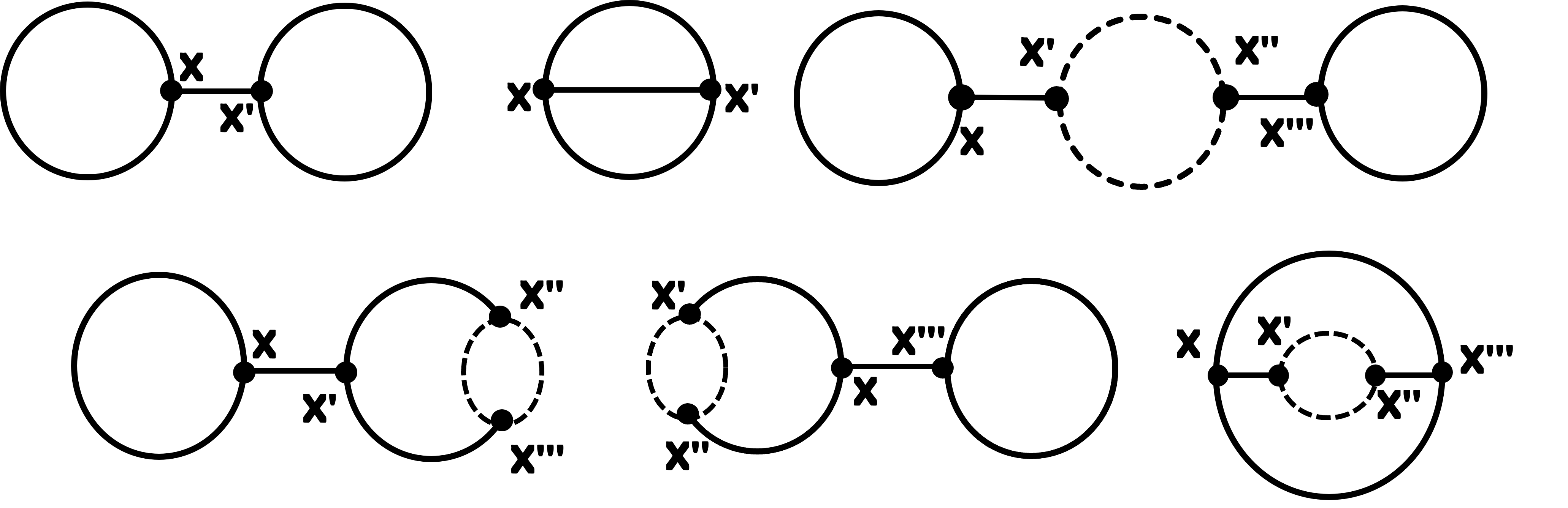
Figure 2: Vacuum diagrams for perturbative computation of $\langle\phi^{3}(x)\rangle$ up to three loop. Solid and dashed lines represent respectively the scalar and the fermion. All primed vertices are integrated over.

In order to compute $\langle\phi^{3}\rangle$ perturbatively, we shall be dealing with six diagrams at ${\cal O}(\beta)$ and ${\cal O}(\beta g^{2})$ as shown in 2. The first diagram in the in-in or Schwinger-Keldysh formalism outlined in A reads

$$-\frac{3i\beta}{2}\int d^{d}x^{\prime}a^{\prime d}i\Delta(x,x)i\Delta(x^{\prime},x^{\prime})\left(i\Delta_{++}(x,x^{\prime})-i\Delta_{+-}(x,x^{\prime})\right)$$ (23)

Note that the tadpoles of this diagram give divergences from 12, which can be canceled via the one loop tadpole counterterm 13. However, we really do not need to bother ourselves with renormalisation for now, as we are essentially working in a late time long wavelength framework. We shall discuss some renormalisation instead in 4.4, where we need to compute some purely local contributions, in order to compute the dynamically generated mass. The leading secular contribution from any diagram is essentially a non-local one free from any ultraviolet divergences, giving one secular logarithm for each internal line. The local contributions contain $\delta$-functions and consist of divergent plus finite parts. The finite part may contain secular logarithms as well but their power are less than the total number of internal lines.

We recall now that $\eta$ is the final time, B. Thus from A, we have for 23

$$\frac{3i\beta}{2}\int d^{d}x^{\prime}a^{\prime d}i\Delta(x,x)i\Delta(x^{\prime},x^{\prime})\left(i\Delta_{+-}(x,x^{\prime})-i\Delta_{-+}(x,x^{\prime})\right)$$

$$=\frac{3i\beta H^{4}}{2^{5}\pi^{4}}\ln a\times\int d\eta^{\prime}a^{\prime 4}\ln a^{\prime}\left(i\Delta_{+-}(k=0,\eta,\eta^{\prime})-i\Delta_{-+}(k=0,\eta,\eta^{\prime})\right)=-\frac{\beta H^{2}}{2^{6}\pi^{4}}\ln^{3}a\,+\,{\cal O}(\ln^{2}a)$$ (24)

where we have used the finite part of 12 and the ingredients of B, derived using the spatial momentum space. We note that the three internal lines of the diagram has yielded the cubic power of the late time secular logarithm at the leading order.

The in-in amplitude for the the second diagram of 2 reads

$$-i\beta\int d^{4}x^{\prime}a^{\prime 4}\left(i\Delta^{3}_{++}(x,x^{\prime})-i\Delta^{3}_{+-}(x,x^{\prime})\right)$$ (25)

Using the expressions given towards the end of A, and the spatial momentum space as discussed in B, we have after some algebra the leading late time result

$$i\beta\int d^{4}x^{\prime}a^{\prime 4}\left(i\Delta^{3}_{+-}(x,x^{\prime})-i\Delta^{3}_{-+}(x,x^{\prime})\right)=-\frac{\beta H^{2}}{2^{4}\times 3\pi^{4}}\ln^{3}a$$ (26)

The third of 2 contains the Yukawa interaction. Recall that we shall work only with the local part of the fermion loop here (cf., the discussion towards the end of 2). This means we may ignore the self-energies due to the fermion Wightman functions, $iS_{\pm\mp}(x,x^{\prime})$. Thus the relevant contribution reads

$$3i\beta g^{2}i\Delta(x,x){\rm Tr}\int d^{4}x^{\prime}d^{4}x^{\prime\prime}d^{4}x^{\prime\prime\prime}(a^{\prime}a^{\prime\prime}a^{\prime\prime\prime})^{4}i\Delta(x^{\prime\prime\prime},x^{\prime\prime\prime})\left[i\Delta_{-+}(x,x^{\prime})i\Delta_{++}(x^{\prime\prime},x^{\prime\prime\prime})iS^{2}_{++}(x^{\prime},x^{\prime\prime})\right.$$

$$\left.+i\Delta_{+-}(x,x^{\prime})i\Delta_{-+}(x^{\prime\prime},x^{\prime\prime\prime})iS^{2}_{--}(x^{\prime},x^{\prime\prime})-i\Delta_{-+}(x,x^{\prime})i\Delta_{+-}(x^{\prime\prime},x^{\prime\prime\prime})iS^{2}_{++}(x^{\prime},x^{\prime\prime})-i\Delta_{+-}(x,x^{\prime})i\Delta_{--}(x^{\prime\prime},x^{\prime\prime\prime})iS^{2}_{--}(x^{\prime},x^{\prime\prime})\right]$$

(27)

It is easy to see that the above integral is non-vanishing only for the temporal hierarchy $\eta^{\prime},\eta^{\prime\prime}\gtrsim\eta^{\prime\prime\prime}$. Using this and the renormalised expression for the scalar self energy due to fermion loop derived towards the end of 2, the above integral becomes

$$\frac{3\beta g^{2}H^{4}}{2^{7}\pi^{6}}\ln a\int d^{4}x^{\prime}d^{4}x^{\prime\prime}d^{4}x^{\prime\prime\prime}(a^{\prime}a^{\prime\prime})a^{\prime\prime\prime 4}\ln a^{\prime\prime\prime}\ln(a^{\prime}a^{\prime\prime})(\partial_{x^{\prime\prime}}^{2}\delta^{4}(x^{\prime}-x^{\prime\prime}))$$

$$\times\left(i\Delta_{+-}(x,x^{\prime})-i\Delta_{-+}(x,x^{\prime})\right)\left(i\Delta_{+-}(x^{\prime\prime},x^{\prime\prime\prime})-i\Delta_{-+}(x^{\prime\prime},x^{\prime\prime\prime})\right)$$ (28)

Integrating 28 now by parts utilising the $\delta$-function, we have

$$\frac{3\beta g^{2}H^{4}}{2^{6}\pi^{6}}\ln a\int d^{4}x^{\prime}d^{4}x^{\prime\prime\prime}a^{\prime\prime\prime 4}\ln a^{\prime\prime\prime}\,\partial^{2}_{x^{\prime}}\left[a^{\prime 2}\ln a^{\prime}\times\left(i\Delta_{+-}(x,x^{\prime})-i\Delta_{-+}(x,x^{\prime})\right)\left(i\Delta_{+-}(x^{\prime},x^{\prime\prime\prime})-i\Delta_{-+}(x^{\prime},x^{\prime\prime\prime})\right)\right]$$

(29)

Let us first evaluate the spatial derivative part, $\partial^{2}_{\vec{x}^{\prime}}$. Introducing the $3$-momentum space as in B, the relevant part of the above integration reads

$$\int d^{3}\vec{x}^{\prime}d^{3}\vec{x}^{\prime\prime\prime}\frac{d^{3}\vec{k}_{1}d^{3}\vec{k}_{2}}{(2\pi)^{6}}\partial^{2}_{\vec{x}^{\prime}}\left[e^{i\vec{k}_{1}\cdot(\vec{x}-\vec{x^{\prime}})}e^{i\vec{k}_{2}\cdot(\vec{x^{\prime}}-\vec{x^{\prime\prime\prime}})}\left(i\Delta_{+-}(k_{1},\eta,\eta^{\prime})-i\Delta_{-+}(k_{1},\eta,\eta^{\prime})\right)\left(i\Delta_{+-}(k_{2},\eta^{\prime},\eta^{\prime\prime\prime})-i\Delta_{-+}(k_{2},\eta^{\prime},\eta^{\prime\prime\prime})\right)\right]$$

$$=-\int d^{3}\vec{x}^{\prime}\frac{d^{3}\vec{k}_{1}}{(2\pi)^{3}}\vec{k}^{2}_{1}e^{i\vec{k}_{1}\cdot(\vec{x}-\vec{x^{\prime}})}\left(i\Delta_{+-}(k_{1},\eta,\eta^{\prime})-i\Delta_{-+}(k_{1},\eta,\eta^{\prime})\right)\left(i\Delta_{+-}(0,\eta^{\prime},\eta^{\prime\prime\prime})-i\Delta_{-+}(0,\eta^{\prime},\eta^{\prime\prime\prime})\right)$$ (30)

We recall that $\left(i\Delta_{+-}(k,\eta,\eta^{\prime})-i\Delta_{-+}(k,\eta,\eta^{\prime})\right)=i/3Ha^{\prime 3}$ at the leading order, irrespective of the value of $k$, B. Performing now the $\vec{x^{\prime}}$ integration gives a $\delta^{3}(\vec{k}_{1})$, forcing thus the integration to vanish, giving us the relevant part of 29,

$$-\frac{3\beta g^{2}H^{4}}{2^{6}\pi^{6}}\ln a\int d^{4}x^{\prime}d^{4}x^{\prime\prime\prime}a^{\prime\prime\prime 4}\ln a^{\prime\prime\prime}\,\partial^{2}_{\eta^{\prime}}\left[a^{\prime 2}\ln a^{\prime}\times\left(i\Delta_{+-}(x,x^{\prime})-i\Delta_{-+}(x,x^{\prime})\right)\left(i\Delta_{+-}(x^{\prime},x^{\prime\prime\prime})-i\Delta_{-+}(x^{\prime},x^{\prime\prime\prime})\right)\right]$$

(31)

Employing the spatial momentum space again, the above integral becomes

$$-\frac{3\beta g^{2}H^{4}}{2^{6}\pi^{6}}\ln a\int d\eta^{\prime}d\eta^{\prime\prime\prime}a^{\prime\prime\prime 4}\ln a^{\prime\prime\prime}\,\partial^{2}_{\eta^{\prime}}\left[a^{\prime 2}\ln a^{\prime}\times\left(i\Delta_{+-}(0,\eta,\eta^{\prime})-i\Delta_{-+}(0,\eta,\eta^{\prime})\right)\left(i\Delta_{+-}(0,\eta^{\prime},\eta^{\prime\prime\prime})-i\Delta_{-+}(0,\eta^{\prime},\eta^{\prime\prime\prime})\right)\right]$$

$$=\frac{\beta g^{2}H^{2}}{2^{6}\times 3\pi^{6}}\ln a\int d\eta^{\prime}d\eta^{\prime\prime\prime}a^{\prime\prime\prime}\ln a^{\prime\prime\prime}\partial^{2}_{\eta^{\prime}}\left(\frac{\ln a^{\prime}}{a^{\prime}}\right)=-\frac{\beta g^{2}H^{2}}{2^{6}\times 3\pi^{6}}\ln a\int\frac{da^{\prime}}{a^{\prime}}\frac{da^{\prime\prime\prime}}{a^{\prime\prime\prime}}\ln a^{\prime\prime\prime}=-\frac{\beta g^{2}H^{2}}{2^{7}\times 9\pi^{6}}\ln^{4}a$$ (32)

where in the last line we have used the temporal hierarchy, $\eta^{\prime}\gtrsim\eta^{\prime\prime\prime}$.

Likewise, the fourth diagram of 2 equals

$$3i\beta g^{2}i\Delta(x,x){\rm Tr}\int d^{4}x^{\prime}d^{4}x^{\prime\prime}d^{4}x^{\prime\prime\prime}(a^{\prime}a^{\prime\prime}a^{\prime\prime\prime})^{4}\left[i\Delta_{-+}(x,x^{\prime})i\Delta_{++}(x^{\prime},x^{\prime\prime})i\Delta_{++}(x^{\prime},x^{\prime\prime\prime})iS^{2}_{++}(x^{\prime\prime},x^{\prime\prime\prime})\right.$$

$$\left.+i\Delta_{-+}(x,x^{\prime})i\Delta_{+-}(x^{\prime},x^{\prime\prime})i\Delta_{+-}(x^{\prime},x^{\prime\prime\prime})iS^{2}_{--}(x^{\prime\prime},x^{\prime\prime\prime})-i\Delta_{+-}(x,x^{\prime})i\Delta_{-+}(x^{\prime},x^{\prime\prime})i\Delta_{-+}(x^{\prime},x^{\prime\prime\prime})iS^{2}_{++}(x^{\prime\prime},x^{\prime\prime\prime})\right.$$

$$\left.-i\Delta_{+-}(x,x^{\prime})i\Delta_{--}(x^{\prime},x^{\prime\prime})i\Delta_{--}(x^{\prime},x^{\prime\prime\prime})iS^{2}_{--}(x^{\prime\prime},x^{\prime\prime\prime})\right]$$ (33)

The above integral is non-vanishing for $\eta^{\prime}\gtrsim\eta^{\prime\prime},\eta^{\prime\prime\prime}$, hence can be written as

$$\frac{3\beta g^{2}H^{2}}{2^{5}\pi^{4}}\ln a\int d^{4}x^{\prime}d^{4}x^{\prime\prime}d^{4}x^{\prime\prime\prime}a^{\prime 4}(a^{\prime\prime}a^{\prime\prime\prime})\ln(a^{\prime\prime}a^{\prime\prime\prime})(\partial^{2}_{x^{\prime\prime\prime}}\delta^{4}(x^{\prime\prime}-x^{\prime\prime\prime}))$$

$$\times\left(i\Delta_{+-}(x,x^{\prime})-i\Delta_{-+}(x,x^{\prime})\right)\left(i\Delta_{+-}(x^{\prime},x^{\prime\prime})i\Delta_{+-}(x^{\prime},x^{\prime\prime\prime})-i\Delta_{-+}(x^{\prime},x^{\prime\prime})i\Delta_{-+}(x^{\prime},x^{\prime\prime\prime})\right)$$

$$=-\frac{3\beta g^{2}H^{2}}{2^{4}\pi^{4}}\ln a\int d^{4}x^{\prime}d^{4}x^{\prime\prime}a^{\prime 4}\partial^{2}_{x^{\prime\prime}}\left[a^{\prime\prime 2}\ln a^{\prime\prime}\left(i\Delta_{+-}(x,x^{\prime})-i\Delta_{-+}(x,x^{\prime})\right)\left(i\Delta^{2}_{+-}(x^{\prime},x^{\prime\prime})-i\Delta^{2}_{-+}(x^{\prime},x^{\prime\prime})\right)\right]$$ (34)

We evaluate the above as earlier. The spatial derivative part of the integral, $\partial^{2}_{\vec{x^{\prime\prime}}}$ vanishes and we obtain by employing the spatial momentum space,

$$-\frac{\beta g^{2}H^{2}}{2^{5}\times 9\pi^{6}}\ln^{4}a$$ (35)

The fifth diagram of 2 equals,

$$3i\beta g^{2}{\rm Tr}\int d^{4}x^{\prime}d^{4}x^{\prime\prime}d^{4}x^{\prime\prime\prime}(a^{\prime}a^{\prime\prime}a^{\prime\prime\prime})^{4}i\Delta(x^{\prime},x^{\prime})\left[i\Delta_{-+}(x,x^{\prime})i\Delta_{-+}(x,x^{\prime\prime})i\Delta_{-+}(x,x^{\prime\prime\prime})iS^{2}_{++}(x^{\prime\prime},x^{\prime\prime\prime})\right.$$

$$\left.+i\Delta_{-+}(x,x^{\prime})i\Delta_{+-}(x,x^{\prime\prime})i\Delta_{+-}(x,x^{\prime\prime\prime})iS^{2}_{--}(x^{\prime\prime},x^{\prime\prime\prime})-i\Delta_{+-}(x,x^{\prime})i\Delta_{-+}(x,x^{\prime\prime})i\Delta_{-+}(x,x^{\prime\prime\prime})iS^{2}_{++}(x^{\prime\prime},x^{\prime\prime\prime})\right.$$

$$\left.-i\Delta_{+-}(x,x^{\prime})i\Delta_{+-}(x,x^{\prime\prime})i\Delta_{+-}(x,x^{\prime\prime\prime})iS^{2}_{--}(x^{\prime\prime},x^{\prime\prime\prime})\right]$$

$$=\frac{3\beta g^{2}H^{2}}{2^{5}\pi^{4}}\int d^{4}x^{\prime}d^{4}x^{\prime\prime}d^{4}x^{\prime\prime\prime}a^{\prime 4}(a^{\prime\prime}a^{\prime\prime\prime})\ln a^{\prime}\ln(a^{\prime\prime}a^{\prime\prime\prime})(\partial^{2}_{x^{\prime\prime\prime}}\delta^{4}(x^{\prime\prime}-x^{\prime\prime\prime}))$$

$$\times\left(i\Delta_{+-}(x,x^{\prime})-i\Delta_{-+}(x,x^{\prime})\right)\left(i\Delta_{+-}(x,x^{\prime\prime})i\Delta_{+-}(x,x^{\prime\prime\prime})-i\Delta_{-+}(x,x^{\prime\prime})i\Delta_{-+}(x,x^{\prime\prime\prime})\right)$$ (36)

The spatial derivative part vanishes as earlier to yield,

$$-\frac{\beta g^{2}H^{2}}{2^{6}\times 3\pi^{6}}\ln^{4}a$$ (37)

The sixth diagram of 2 equals

$$2i\beta g^{2}{\rm Tr}\int d^{4}x^{\prime}d^{4}x^{\prime\prime}d^{4}x^{\prime\prime\prime}(a^{\prime}a^{\prime\prime}a^{\prime\prime\prime})^{4}\left[i\Delta^{2}_{-+}(x,x^{\prime\prime\prime})i\Delta_{-+}(x,x^{\prime})i\Delta_{++}(x^{\prime\prime},x^{\prime\prime\prime})iS^{2}_{++}(x^{\prime},x^{\prime\prime})\right.$$

$$\left.+i\Delta^{2}_{-+}(x,x^{\prime\prime\prime})i\Delta_{+-}(x,x^{\prime})i\Delta_{-+}(x^{\prime\prime},x^{\prime\prime\prime})iS^{2}_{--}(x^{\prime},x^{\prime\prime})-i\Delta^{2}_{+-}(x,x^{\prime\prime\prime})i\Delta_{-+}(x,x^{\prime})i\Delta_{+-}(x^{\prime\prime},x^{\prime\prime\prime})iS^{2}_{++}(x^{\prime},x^{\prime\prime})\right.$$

$$\left.-i\Delta^{2}_{+-}(x,x^{\prime\prime\prime})i\Delta_{+-}(x,x^{\prime})i\Delta_{--}(x^{\prime\prime},x^{\prime\prime\prime})iS^{2}_{--}(x^{\prime},x^{\prime\prime})\right]$$ (38)

For $\eta^{\prime\prime}\gtrsim\eta^{\prime\prime\prime}$, this gives,

$$\frac{\beta g^{2}}{2^{2}\pi^{2}}\int d^{4}x^{\prime}d^{4}x^{\prime\prime}d^{4}x^{\prime\prime\prime}(a^{\prime}a^{\prime\prime})a^{\prime\prime\prime 4}\ln(a^{\prime}a^{\prime\prime})\partial^{2}_{x^{\prime\prime}}\delta^{4}(x^{\prime}-x^{\prime\prime})$$

$$\times\left(i\Delta_{+-}(x,x^{\prime})-i\Delta_{-+}(x,x^{\prime})\right)\left(i\Delta^{2}_{+-}(x,x^{\prime\prime\prime})i\Delta_{+-}(x^{\prime\prime},x^{\prime\prime\prime})-i\Delta^{2}_{-+}(x,x^{\prime\prime\prime})i\Delta_{-+}(x^{\prime\prime},x^{\prime\prime\prime})\right)=-\frac{\beta g^{2}H^{2}}{2^{7}\times 9\pi^{6}}\ln^{4}a$$

(39)

For $\eta^{\prime\prime\prime}\gtrsim\eta^{\prime\prime}$, 38 becomes,

$$\frac{\beta g^{2}}{2^{2}\pi^{2}}\int d^{4}x^{\prime}d^{4}x^{\prime\prime}d^{4}x^{\prime\prime\prime}(a^{\prime}a^{\prime\prime})a^{\prime\prime\prime 4}\ln(a^{\prime}a^{\prime\prime})\partial^{2}_{x^{\prime\prime}}\delta^{4}(x^{\prime}-x^{\prime\prime})$$

$$\times\left(i\Delta^{2}_{+-}(x,x^{\prime\prime\prime})-i\Delta^{2}_{-+}(x,x^{\prime\prime\prime})\right)\left(i\Delta_{+-}(x,x^{\prime})i\Delta_{+-}(x^{\prime\prime\prime},x^{\prime\prime})-i\Delta_{-+}(x,x^{\prime})i\Delta_{-+}(x^{\prime\prime\prime},x^{\prime\prime})\right)=-\frac{\beta g^{2}H^{2}}{2^{6}\times 9\pi^{6}}\ln^{4}a$$

(40)

where we have also used above $i\Delta_{-+}(x^{\prime\prime},x^{\prime\prime\prime})=i\Delta_{+-}(x^{\prime\prime\prime},x^{\prime\prime})$.

Adding the above with 39, the final result for 38 follows. Also, combining this with 24, 26, 32, 35 and 37, we obtain the perturbative result for $\langle\phi^{3}\rangle$ in terms of the leading powers of the secular logarithms

$$\langle\phi^{3}\rangle=-\frac{\beta H^{2}}{2^{6}\times 3\pi^{4}}7\ln^{3}a-\frac{\beta g^{2}H^{2}}{2^{6}\times 9\pi^{6}}7\ln^{4}a+\,{\cal O}(\lambda\beta g^{2})$$ (41)

3.2 Computation of $\langle\phi^{2}\rangle$

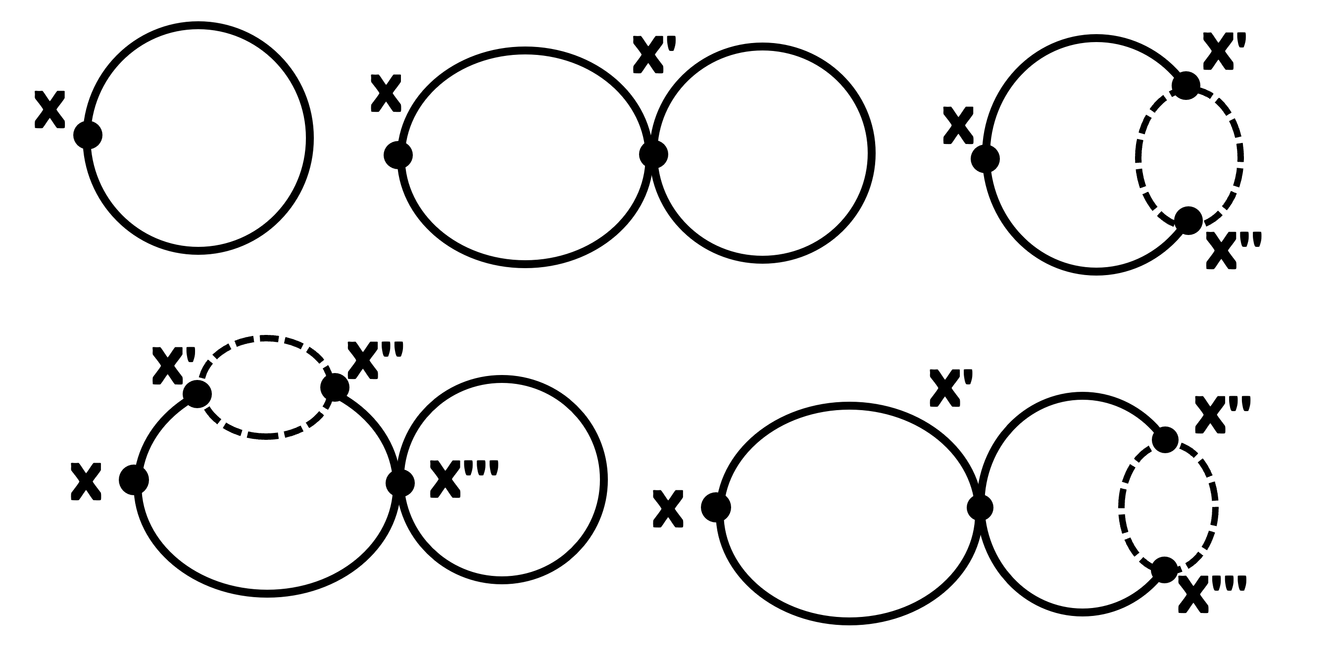
Figure 3: Feynman diagrams for perturbative computation of $\langle\phi^{2}(x)\rangle$ up to three loop. Solid and dashed lines respectively represent the scalar and fermions. All primed vertices are integrated over.

We shall compute the five loop diagrams for the perturbative $\langle\phi^{2}\rangle$, for free theory, ${\cal O}(\lambda)$, ${\cal O}(g^{2})$ and ${\cal O}(\lambda g^{2})$, as shown in 3. The lowest order or free theory value for $\langle\phi^{2}\rangle$ is given by the coincidence limit of any of the four propagators, given by 12 or 115,

$$\frac{H^{2}}{2^{2}\pi^{2}}\ln a$$ (42)

At ${\cal O}(\lambda)$, i.e. the second of 3, we have

$$-\frac{i\lambda}{2}\int d^{4}x^{\prime}a^{\prime 4}i\Delta(x^{\prime},x^{\prime})\left[i\Delta^{2}_{++}(x,x^{\prime})-i\Delta^{2}_{+-}(x,x^{\prime})\right]$$ (43)

After employing the spatial momentum space, its leading late time secular expression equals

$$-\frac{\lambda H^{2}}{2^{4}\times 9\pi^{4}}\ln^{3}a$$ (44)

At ${\cal O}(g^{2})$, i.e. the third of 3, we have following the steps described in the preceding section

$$-2g^{2}{\rm Tr}\int d^{4}x^{\prime}a^{\prime 4}\left[i\Delta_{-+}(x,x^{\prime})i\Delta_{-+}(x,x^{\prime\prime})iS^{2}_{++}(x^{\prime},x^{\prime\prime})+i\Delta_{+-}(x,x^{\prime})i\Delta_{+-}(x,x^{\prime\prime})iS^{2}_{--}(x^{\prime},x^{\prime\prime})\right]$$

$$=-\frac{ig^{2}}{2^{2}\pi^{2}}\int d^{4}x^{\prime}d^{4}x^{\prime\prime}a^{\prime}a^{\prime\prime}\ln(a^{\prime}a^{\prime\prime})(\partial^{2}_{x^{\prime\prime}}\delta^{4}(x^{\prime}-x^{\prime\prime}))\left(i\Delta_{+-}(x,x^{\prime})i\Delta_{+-}(x,x^{\prime\prime})-i\Delta_{-+}(x,x^{\prime})i\Delta_{-+}(x,x^{\prime\prime})\right)$$

$$=\frac{g^{2}H^{2}}{2^{2}\times 3\pi^{4}}\ln^{2}a$$ (45)

where we have taken the local part of the fermion loop as earlier.

The fourth of 3 which is ${\cal O}(\lambda g^{2})$, reads

$$i\lambda g^{2}{\rm Tr}\int d^{4}x^{\prime}d^{4}x^{\prime\prime}d^{4}x^{\prime\prime\prime}(a^{\prime}a^{\prime\prime}a^{\prime\prime\prime})^{4}i\Delta(x^{\prime\prime\prime},x^{\prime\prime\prime})\left[i\Delta_{-+}(x,x^{\prime})i\Delta_{-+}(x,x^{\prime\prime\prime})i\Delta_{++}(x^{\prime\prime},x^{\prime\prime\prime})iS^{2}_{++}(x^{\prime},x^{\prime\prime})\right.$$

$$\left.+i\Delta_{+-}(x,x^{\prime})i\Delta_{-+}(x,x^{\prime\prime\prime})i\Delta_{-+}(x^{\prime\prime},x^{\prime\prime\prime})iS^{2}_{--}(x^{\prime},x^{\prime\prime})-i\Delta_{-+}(x,x^{\prime})i\Delta_{+-}(x,x^{\prime\prime\prime})i\Delta_{+-}(x^{\prime\prime},x^{\prime\prime\prime})iS^{2}_{++}(x^{\prime},x^{\prime\prime})\right.$$

$$\left.-i\Delta_{+-}(x,x^{\prime})i\Delta_{+-}(x,x^{\prime\prime\prime})i\Delta_{--}(x^{\prime\prime},x^{\prime\prime\prime})iS^{2}_{--}(x^{\prime},x^{\prime\prime})\right]$$

$$=\frac{\lambda g^{2}H^{2}}{2^{5}\pi^{4}}\int d^{4}x^{\prime}d^{4}x^{\prime\prime}d^{4}x^{\prime\prime\prime}(a^{\prime}a^{\prime\prime})a^{\prime\prime\prime 4}\ln a^{\prime\prime\prime}\ln(a^{\prime}a^{\prime\prime})(\partial^{2}_{x^{\prime\prime}}\delta^{4}(x^{\prime}-x^{\prime\prime}))\left[i\Delta_{-+}(x,x^{\prime})i\Delta_{-+}(x,x^{\prime\prime\prime})i\Delta_{++}(x^{\prime\prime},x^{\prime\prime\prime})\right.$$

$$\left.-i\Delta_{+-}(x,x^{\prime})i\Delta_{-+}(x,x^{\prime\prime\prime})i\Delta_{-+}(x^{\prime\prime},x^{\prime\prime\prime})-i\Delta_{-+}(x,x^{\prime})i\Delta_{+-}(x,x^{\prime\prime\prime})i\Delta_{+-}(x^{\prime\prime},x^{\prime\prime\prime})+i\Delta_{+-}(x,x^{\prime})i\Delta_{+-}(x,x^{\prime\prime\prime})i\Delta_{--}(x^{\prime\prime},x^{\prime\prime\prime})\right]$$

(46)

For $\eta^{\prime\prime}\gtrsim\eta^{\prime\prime\prime}$, the above becomes

$$\frac{\lambda g^{2}H^{2}}{2^{5}\pi^{4}}\int d^{4}x^{\prime}d^{4}x^{\prime\prime}d^{4}x^{\prime\prime\prime}(a^{\prime}a^{\prime\prime})a^{\prime\prime\prime 4}\ln a^{\prime\prime\prime}\ln(a^{\prime}a^{\prime\prime})(\partial^{2}_{x^{\prime\prime}}\delta^{4}(x^{\prime}-x^{\prime\prime}))\left(i\Delta_{+-}(x,x^{\prime})-i\Delta_{-+}(x,x^{\prime})\right)$$

$$\times\left(i\Delta_{+-}(x,x^{\prime\prime\prime})i\Delta_{+-}(x^{\prime\prime},x^{\prime\prime\prime})-i\Delta_{-+}(x,x^{\prime\prime\prime})i\Delta_{-+}(x^{\prime\prime},x^{\prime\prime\prime})\right)=-\frac{\lambda g^{2}H^{2}}{2^{7}\times 9\pi^{6}}\frac{\ln^{4}a}{3}$$ (47)

For $\eta^{\prime\prime}\lesssim\eta^{\prime\prime\prime}$ on the other hand, we have

$$\frac{\lambda g^{2}H^{2}}{2^{5}\pi^{4}}\int d^{4}x^{\prime}d^{4}x^{\prime\prime}d^{4}x^{\prime\prime\prime}(a^{\prime}a^{\prime\prime})a^{\prime\prime\prime 4}\ln a^{\prime\prime\prime}\ln(a^{\prime}a^{\prime\prime})(\partial^{2}_{x^{\prime\prime}}\delta^{4}(x^{\prime}-x^{\prime\prime}))\left(i\Delta_{+-}(x,x^{\prime\prime\prime})-i\Delta_{-+}(x,x^{\prime\prime\prime})\right)$$

$$\times\left(i\Delta_{+-}(x,x^{\prime})i\Delta_{-+}(x^{\prime\prime},x^{\prime\prime\prime})-i\Delta_{-+}(x,x^{\prime})i\Delta_{+-}(x^{\prime\prime},x^{\prime\prime\prime})\right)=-\frac{\lambda g^{2}H^{2}}{2^{7}\times 9\pi^{6}}\ln^{4}a$$ (48)

Combining the above with 47, the desired result follows.

Finally, for the last of 3, we have the integral

$$i\lambda g^{2}{\rm Tr}\int d^{4}x^{\prime}d^{4}x^{\prime\prime}d^{4}x^{\prime\prime\prime}(a^{\prime}a^{\prime\prime}a^{\prime\prime\prime})^{4}\left[i\Delta_{-+}^{2}(x,x^{\prime})i\Delta_{++}(x^{\prime},x^{\prime\prime})i\Delta_{++}(x^{\prime},x^{\prime\prime\prime})iS^{2}_{++}(x^{\prime\prime},x^{\prime\prime\prime})\right.$$

$$\left.+i\Delta_{-+}^{2}(x,x^{\prime})i\Delta_{+-}(x^{\prime},x^{\prime\prime})i\Delta_{+-}(x^{\prime},x^{\prime\prime\prime})iS^{2}_{--}(x^{\prime\prime},x^{\prime\prime\prime})-i\Delta_{+-}^{2}(x,x^{\prime})i\Delta_{-+}(x^{\prime},x^{\prime\prime})i\Delta_{-+}(x^{\prime},x^{\prime\prime\prime})iS^{2}_{++}(x^{\prime\prime},x^{\prime\prime\prime})\right.$$

$$\left.-i\Delta_{+-}^{2}(x,x^{\prime})i\Delta_{--}(x^{\prime},x^{\prime\prime})i\Delta_{--}(x^{\prime},x^{\prime\prime\prime})iS^{2}_{--}(x^{\prime\prime},x^{\prime\prime\prime})\right]$$

$$=\frac{\lambda g^{2}}{2^{3}\pi^{2}}\int d^{4}x^{\prime}d^{4}x^{\prime\prime}d^{4}x^{\prime\prime\prime}a^{\prime 4}a^{\prime\prime}a^{\prime\prime\prime}\ln(a^{\prime\prime}a^{\prime\prime\prime})(\partial^{2}_{x^{\prime\prime\prime}}\delta^{4}(x^{\prime\prime}-x^{\prime\prime\prime}))\left[i\Delta^{2}_{-+}(x,x^{\prime})i\Delta_{++}(x^{\prime},x^{\prime\prime})i\Delta_{++}(x^{\prime},x^{\prime\prime\prime})\right.$$

$$\left.-i\Delta^{2}_{-+}(x,x^{\prime})i\Delta_{+-}(x^{\prime},x^{\prime\prime})i\Delta_{+-}(x^{\prime},x^{\prime\prime\prime})-i\Delta^{2}_{+-}(x,x^{\prime})i\Delta_{-+}(x^{\prime},x^{\prime\prime})i\Delta_{-+}(x^{\prime},x^{\prime\prime\prime})+i\Delta^{2}_{+-}(x,x^{\prime})i\Delta_{--}(x^{\prime},x^{\prime\prime})i\Delta_{--}(x^{\prime},x^{\prime\prime\prime})\right]$$

(49)

The above integral vanishes for $\eta^{\prime}\lesssim\eta^{\prime\prime},\eta^{\prime\prime\prime}$. Accordingly it becomes,

$$\frac{\lambda g^{2}}{2^{3}\pi^{2}}\int d^{4}x^{\prime}d^{4}x^{\prime\prime}d^{4}x^{\prime\prime\prime}a^{\prime 4}(a^{\prime\prime}a^{\prime\prime\prime})\ln(a^{\prime\prime}a^{\prime\prime\prime})(\partial^{2}_{x^{\prime\prime\prime}}\delta^{4}(x^{\prime\prime}-x^{\prime\prime\prime}))$$

$$\times\left(i\Delta^{2}_{+-}(x,x^{\prime})-i\Delta^{2}_{-+}(x,x^{\prime})\right)\left(i\Delta_{+-}(x^{\prime},x^{\prime\prime})i\Delta_{+-}(x^{\prime},x^{\prime\prime\prime})-i\Delta_{-+}(x^{\prime},x^{\prime\prime})i\Delta_{-+}(x^{\prime},x^{\prime\prime\prime})\right)=-\frac{\lambda g^{2}H^{2}}{2^{6}\times 9\pi^{6}}\ln^{4}a$$

(50)

Combining now 42, 44, 45, 47, 48, 50, we have

$$\langle\phi^{2}\rangle=\frac{H^{2}}{2^{2}\pi^{2}}\ln a-\frac{\lambda H^{2}}{2^{4}\times 9\pi^{4}}\ln^{3}a+\frac{g^{2}H^{2}}{2^{2}\times 3\pi^{4}}\ln^{2}a-\frac{\lambda g^{2}H^{2}}{2^{6}\times 9\pi^{6}}\frac{5\ln^{4}a}{3}+{\cal O}(\lambda^{2}g^{2})$$ (51)

3.3 Computation of $\langle\overline{\Psi}\Psi\rangle$

Figure 4: Loop diagrams for the perturbative computation of $\langle\bar{\Psi}\Psi\rangle$. Dashed and solid lines stand for fermion and scalar respectively. All primed vertices are integrated over. Also for the free theory, $\langle\bar{\Psi}\Psi\rangle=0$, as is evident from 16.

There are four diagrams at ${\cal O}(\beta g)$ and ${\cal O}(\beta g\lambda)$ corresponding to $\langle\bar{\Psi}\Psi(x)\rangle$ up to three loop. For the free theory $\langle\bar{\Psi}\Psi(x)\rangle=-{\rm Tr}\,iS(x,x)=0$, follows from 16. We also note that the fermionic field appearing at the observed vertex at $x$ must be of $+$ kind, in the in-in formalism. The first of 4 then gives, recalling that we are interested only in the local contribution from a closed fermion loop,

$$-\frac{\beta g}{2}\int d^{4}x^{\prime}d^{4}x^{\prime\prime}(a^{\prime}a^{\prime\prime})^{4}{\rm Tr}(iS^{2}_{++}(x,x^{\prime}))\left(i\Delta_{++}(x^{\prime},x^{\prime\prime})-i\Delta_{+-}(x^{\prime},x^{\prime\prime})\right)i\Delta(x^{\prime\prime},x^{\prime\prime})$$

$$=-\frac{i\beta gH^{2}}{2^{6}\pi^{4}}\int d^{4}x^{\prime}d^{4}x^{\prime\prime}\frac{a^{\prime}a^{\prime\prime 4}}{a^{3}}\ln(aa^{\prime})\ln a^{\prime\prime}(\partial_{x^{\prime}}^{2}\delta^{4}(x-x^{\prime}))\left(i\Delta_{+-}(x^{\prime},x^{\prime\prime})-i\Delta_{-+}(x^{\prime},x^{\prime\prime})\right)$$

$$=\frac{i\beta gH^{2}}{2^{5}\pi^{4}}\int d\eta^{\prime\prime}a^{\prime\prime 4}\ln a^{\prime\prime}\partial^{2}_{\eta}\left(\frac{\ln a}{a^{2}}\left(i\Delta_{+-}(0,\eta,\eta^{\prime\prime})-i\Delta_{-+}(0,\eta,\eta^{\prime\prime})\right)\right)$$

$$=\frac{i\beta gH}{2^{5}\pi^{4}}\int da^{\prime\prime}a^{\prime\prime 2}\ln a^{\prime\prime}\partial^{2}_{\eta}\left(\frac{\ln a}{a^{2}}\times\frac{i}{3Ha^{\prime\prime 3}}\right)=-\frac{\beta gH^{2}}{2^{5}\times 3\pi^{4}}\ln^{3}a$$ (52)

The second of 4 reads

$$\frac{i\lambda\beta g}{4}\int d^{4}x^{\prime}d^{4}x^{\prime\prime}d^{4}x^{\prime\prime\prime}(a^{\prime}a^{\prime\prime}a^{\prime\prime\prime})^{4}i\Delta(x^{\prime\prime},x^{\prime\prime})i\Delta(x^{\prime\prime\prime},x^{\prime\prime\prime}){\rm Tr}(iS^{2}_{++}(x,x^{\prime}))$$

$$\times\left(i\Delta_{+-}(x^{\prime},x^{\prime\prime})-i\Delta_{-+}(x^{\prime},x^{\prime\prime})\right)\left(i\Delta_{+-}(x^{\prime\prime},x^{\prime\prime\prime})-i\Delta_{-+}(x^{\prime\prime},x^{\prime\prime\prime})\right)$$

$$=\frac{\lambda\beta gH^{4}}{2^{9}\times\pi^{6}}\int d^{4}x^{\prime}d^{4}x^{\prime\prime}d^{4}x^{\prime\prime\prime}(a^{\prime\prime}a^{\prime\prime\prime})^{4}\ln a^{\prime\prime}\ln a^{\prime\prime\prime}\left(\frac{a^{\prime}\ln(aa^{\prime})}{a^{3}}\right)\partial^{2}_{x^{\prime}}\delta^{4}(x-x^{\prime})$$

$$\times\left(i\Delta_{+-}(x^{\prime},x^{\prime\prime})-i\Delta_{-+}(x^{\prime},x^{\prime\prime})\right)\left(i\Delta_{+-}(x^{\prime\prime},x^{\prime\prime\prime})-i\Delta_{-+}(x^{\prime\prime},x^{\prime\prime\prime})\right)=\frac{\lambda\beta gH^{2}}{2^{10}\times 9\pi^{6}}\ln^{5}a$$ (53)

The third diagram of 4 gives

$$\frac{i\lambda\beta g}{4}\int d^{4}x^{\prime}d^{4}x^{\prime\prime}d^{4}x^{\prime\prime\prime}(a^{\prime}a^{\prime\prime}a^{\prime\prime\prime})^{4}i\Delta(x^{\prime\prime\prime},x^{\prime\prime\prime}){\rm Tr}(iS^{2}_{++}(x,x^{\prime}))$$

$$\times\left(i\Delta_{+-}(x^{\prime},x^{\prime\prime})-i\Delta_{-+}(x^{\prime},x^{\prime\prime})\right)\left(i\Delta^{2}_{+-}(x^{\prime\prime},x^{\prime\prime\prime})-i\Delta^{2}_{-+}(x^{\prime\prime},x^{\prime\prime\prime})\right)$$

$$=\frac{\lambda\beta gH^{2}}{2^{7}\pi^{4}}\int d^{4}x^{\prime}d^{4}x^{\prime\prime}d^{4}x^{\prime\prime\prime}(a^{\prime\prime}a^{\prime\prime\prime})^{4}\ln a^{\prime\prime\prime}\left(\frac{a^{\prime}}{a^{3}}\ln(aa^{\prime})\right)(\partial^{2}_{x^{\prime}}\delta^{4}(x-x^{\prime}))$$

$$\times\left(i\Delta_{+-}(x^{\prime},x^{\prime\prime})-i\Delta_{-+}(x^{\prime},x^{\prime\prime})\right)\left(i\Delta^{2}_{+-}(x^{\prime\prime},x^{\prime\prime\prime})-i\Delta^{2}_{-+}(x^{\prime\prime},x^{\prime\prime\prime})\right)=\frac{\lambda\beta gH^{2}}{2^{8}\times 9\pi^{6}}\frac{\ln^{5}a}{3}$$ (54)

Finally, the last diagram of 4 reads

$$\frac{i\lambda\beta g}{6}\int d^{4}x^{\prime}d^{4}x^{\prime\prime}d^{4}x^{\prime\prime\prime}(a^{\prime}a^{\prime\prime}a^{\prime\prime\prime})^{4}{\rm Tr}(iS^{2}_{++}(x,x^{\prime}))\left(i\Delta_{+-}(x^{\prime},x^{\prime\prime})-i\Delta_{-+}(x^{\prime},x^{\prime\prime})\right)\left(i\Delta^{3}_{+-}(x^{\prime\prime},x^{\prime\prime\prime})-i\Delta^{3}_{-+}(x^{\prime\prime},x^{\prime\prime\prime})\right)$$

$$=\frac{\lambda\beta gH^{2}}{2^{8}\times 9\pi^{6}}\frac{\ln^{5}a}{3}$$ (55)

Combining now 42, 44, 45, 47, 48, 50, we have

$$\langle\bar{\psi}\psi\rangle=-\frac{\beta gH^{2}}{2^{5}\times 3\pi^{4}}\ln^{3}a+\frac{\lambda\beta gH^{2}}{2^{10}\times 9\pi^{6}}\frac{11\ln^{5}a}{3}+{\cal O}(\lambda^{2}\beta g)$$ (56)

The above result, along with 41 and 51 completes our perturbative computation associated with $\langle\phi\rangle$. We next wish to resum this result below in order to find out a non-perturbative expression for the same.

3.4 Resummation and non-perturbative $\langle\phi\rangle$

Substituting now 41, 51 and 56 into 22, we have for the leading secular logarithms up to the order of the perturbation theory we are interested in,

$$\frac{d\langle\bar{\phi}\rangle}{d{\cal N}}+\frac{\bar{\beta}{\cal N}}{2^{3}\times 3\pi^{2}}-\left(\frac{\bar{\beta}g^{2}}{2^{5}\times 9\pi^{4}}+\frac{11\lambda\bar{\beta}}{2^{7}\times 27\pi^{4}}\right){\cal N}^{3}+\frac{\lambda\bar{\beta}g^{2}}{2^{10}\times 9\pi^{6}}\frac{11{\cal N}^{5}}{9}=0$$ (57)

where ${\cal N}=Ht$ is the number of $e$-foldings, $\bar{\beta}=\beta/H$ and $\bar{\phi}=\phi/H$ are dimensionless. Integrating, we have the late time perturbative result

$$\langle\bar{\phi}\rangle=-\frac{\bar{\beta}{\cal N}^{2}}{2^{4}\times 3\pi^{2}}+\left(\frac{\bar{\beta}g^{2}}{2^{7}\times 9\pi^{4}}+\frac{11\lambda\bar{\beta}}{2^{9}\times 27\pi^{4}}\right){\cal N}^{4}-\frac{\lambda\bar{\beta}g^{2}}{2^{10}\times 9\pi^{6}}\frac{11{\cal N}^{6}}{54}$$ (58)

The $g=0$ part of the above equation has also been obtained by directly computing the tadpoles in the IR limit in C, for the sake of consistency. They match exactly. This shows that integrating any vacuum diagram considered here basically corresponds to attaching an external line to the vertex at $x$, and then replacing the original vertex at $x$ by a dummy vertex $x^{\prime}$ and labelling the new external point on the propagator by $x$, so that the diagrams of 11 are generated eventually. Similar argument holds as well when we include the Yukawa interaction.

Defining now a new variable $\langle\bar{\phi}\rangle=-\langle\varphi\rangle$ in 57, we have

$$\frac{d\langle{\varphi}\rangle}{d{\cal N}}=\frac{\bar{\beta}{\cal N}}{2^{3}\times 3\pi^{2}}-\left(\frac{\bar{\beta}g^{2}}{2^{5}\times 9\pi^{4}}+\frac{11\lambda\bar{\beta}}{2^{7}\times 27\pi^{4}}\right){\cal N}^{3}+\frac{\lambda\bar{\beta}g^{2}}{2^{10}\times 9\pi^{6}}\frac{11{\cal N}^{5}}{9}$$ (59)

Following e.g. [50, 51], we wish to integrate the above equation by promoting the $e$-folding ${\cal N}$ to non-perturbative level via inverting 58 by iteratively using the same into itself. Keeping in mind the relevant order of the perturbative theory, we have after some algebra,

$${\cal N}=\frac{2^{2}\sqrt{3}\pi}{\overline{\beta}^{1/2}}\langle\varphi\rangle^{1/2}+\frac{4\sqrt{3}\pi\langle\varphi\rangle^{3/2}}{\bar{\beta}^{3/2}}\left(g^{2}+\frac{11\lambda}{12}\right)+\frac{\lambda g^{2}\pi\langle\varphi\rangle^{5/2}}{\bar{\beta}^{5/2}}\frac{407}{6\sqrt{3}}$$ (60)

which we substitute into 59 to have,

$$\frac{d\langle\varphi\rangle}{d{\cal N}}=\frac{\bar{\beta}^{1/2}\langle\varphi\rangle^{1/2}}{2\sqrt{3}\pi}-\frac{\sqrt{3}\langle\varphi\rangle^{3/2}}{2\pi\bar{\beta}^{1/2}}\left(g^{2}+\frac{11\lambda}{12}\right)-\frac{649\lambda g^{2}}{144\sqrt{3}\pi}\frac{\langle\varphi\rangle^{5/2}}{\bar{\beta}^{3/2}}$$ (61)

Integrating the above equation, we find as ${\cal N}\gg 1$,

$$\langle\bar{\phi}\rangle=-\langle\varphi\rangle=\frac{108\bar{\beta}}{649\lambda g^{2}}\left(g^{2}+\frac{11\lambda}{12}\right)\left[1-\left(1+\frac{649\lambda g^{2}}{162\left(g^{2}+\frac{11\lambda}{12}\right)^{2}}\right)^{1/2}\right]$$ (62)

The above expression is real, vanishes as $\bar{\beta}\to 0$ and flips sign if the cubic coupling does so. On the other hand, we have as $g\to 0$,

$$\langle\bar{\phi}\rangle_{g\to 0}=-0.364\times\frac{\bar{\beta}}{\lambda}$$ (63)

The numerical factor $0.364$ appearing above is slightly smaller than the one found in [52] via direct computation of $\langle\phi\rangle$, using the exact propagators. This corresponds to a trivial error of overcounting a factor of $1/3$ there, while computing the third diagram of 11. (The leading secular expressions for the rest of the diagrams match exactly with that of [52]). Evidently, there is no such mismatch actually, as has been substantiated by the explicit IR effective computations for the tadpoles in C. We also note from 1 that the classical minima of the tree level potential is located at $-3\bar{\beta}/\lambda$, approximately one order of magnitude less than 63. Thus these results indeed manifest strong quantum fluctuations.

62 is one of the main results of this paper. We have plotted the variations of $\langle\bar{\phi}\rangle$ with respect to different coupling parameters in 5. We have also plotted the variation of the same with respect to the number of $e$-foldings in 6. 5 shows that turning on the Yukawa interaction reduces the magnitude of $\langle\bar{\phi}\rangle$. A non-perturbative $\langle\bar{\phi}\rangle$ may effectively act as a cosmological constant at late times. We refer our reader to [52] for an estimation of backreaction due to it. This completes our discussion on the one point function. We now wish to do similar computations for the two point function $\langle\phi^{2}\rangle$ below.

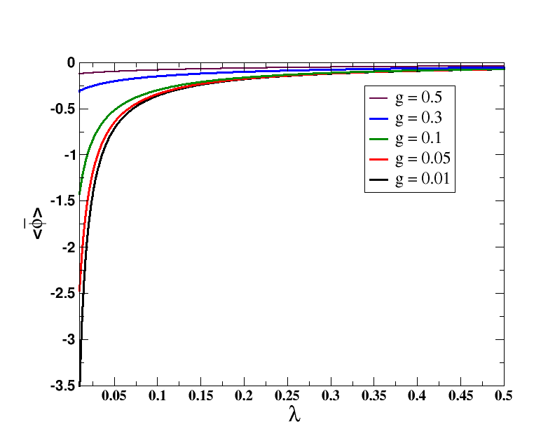
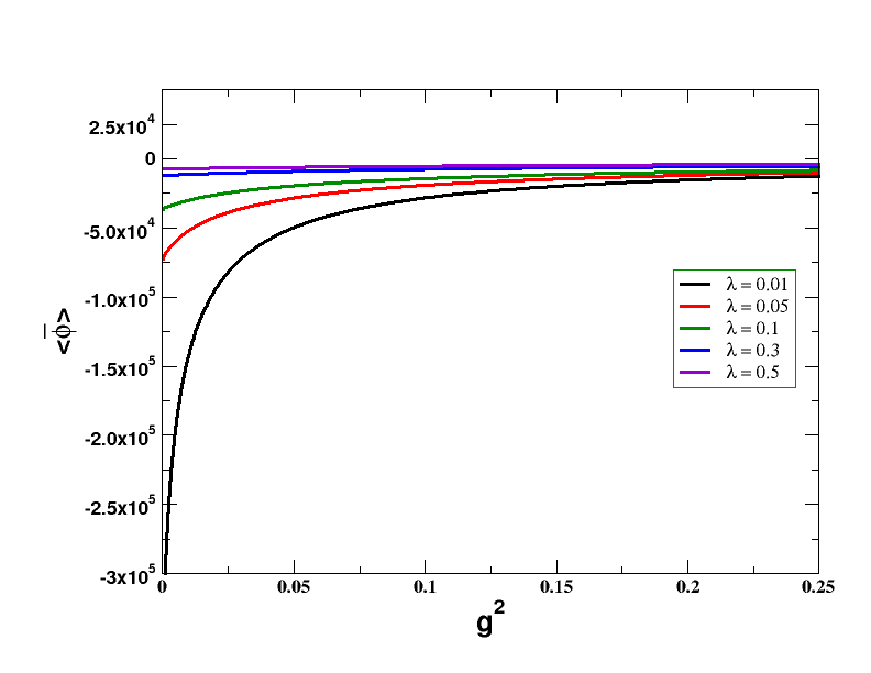
Figure 5: Variation of the non-perturbative $\langle\bar{\phi}\rangle$, 62, with respect to different couplings. Note that it increases with the increasing cubic coupling as is evident from 62, whereas decreases with both increasing quartic and Yukawa couplings. We have taken $\bar{\beta}$ to be positive here. For its negative value, $\langle\bar{\phi}\rangle$ becomes positive.

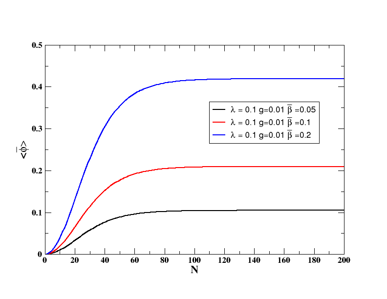
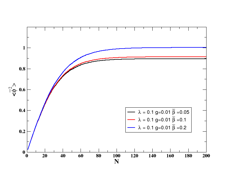
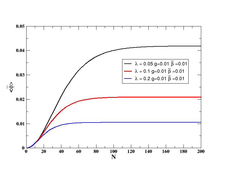
Figure 6: Variation of $\langle\bar{\phi}\rangle$ with respect to the number of $e$-foldings, ${\cal N}$, found from 61 for different values of the couplings.

4 Perturbative computation of $\langle\phi^{2}\rangle$, its resummation and the dynamical mass generation

Taking once again the late time and large scale limit of 21, multiplying it with the scalar $\phi(x)$, and taking the expectation value with respect to the initial Bunch-Davies vacuum, we have in the Heisenberg picture

$$\frac{d\langle\phi^{2}(x)\rangle}{d{\cal N}}=\frac{H^{2}}{4\pi^{2}}-\frac{2}{3H^{2}}\left[\frac{\lambda}{6}\langle\phi^{4}(x)\rangle+\frac{\beta}{2}\langle\phi^{3}(x)\rangle+g\langle\bar{\psi}\psi\phi(x)\rangle\right]$$ (64)

where ${\cal N}=Ht$ is the number of $e$-foldings as earlier and the first term on the right hand side of the above equation corresponds to the free theory result, 115. Setting $\bar{\beta}=0=g$ and employing the Hartree approximation, $\langle\phi^{4}(x)\rangle=3\langle\phi^{2}(x)\rangle^{2}$, one finds the non-perturbative result, $\langle\phi^{2}(x)\rangle\sim\lambda^{-1/2}$ [56]. This result basically contains resummed superdaisy diagrams for the bubble self energy corresponding to the quartic self interaction. Note that in the Hartree approximation the function $\langle\phi^{2}(x)\rangle^{2}$ is purely local, in the sense that it does not contain any integration over spacetime. Accordingly, it indicates the generation of a dynamical scalar mass of order $\lambda^{1/2}$ at late times, even though the scalar field was massless to begin with.

We wish to find out a resummed expression for $\langle\phi^{2}(x)\rangle$ appearing in 64. The correlators appearing in 64 will contain contributions from various loops, like self energies. Such loops can be purely local, purely non-local or mixed type. A local contribution corresponds to the scenario when all the vertices of a self energy loop shrinks to a single point, by the virtue of a $\delta$-function, often divergent requiring renormalisation. A non-local self energy on the other hand, does not contain any such $\delta$-function, and it contains contribution of integrals over spacetime. Both self energies show secular divergences, although the non-local part, as we have mentioned in the preceding section, usually contains greater power of the secular logarithm compared to that of the local part. We wish to resum below both types of these self energies. The local part in particular, will give us the dynamically generated mass of the scalar field at late times.

4.1 Perturbative computation of $\langle\phi^{4}\rangle$

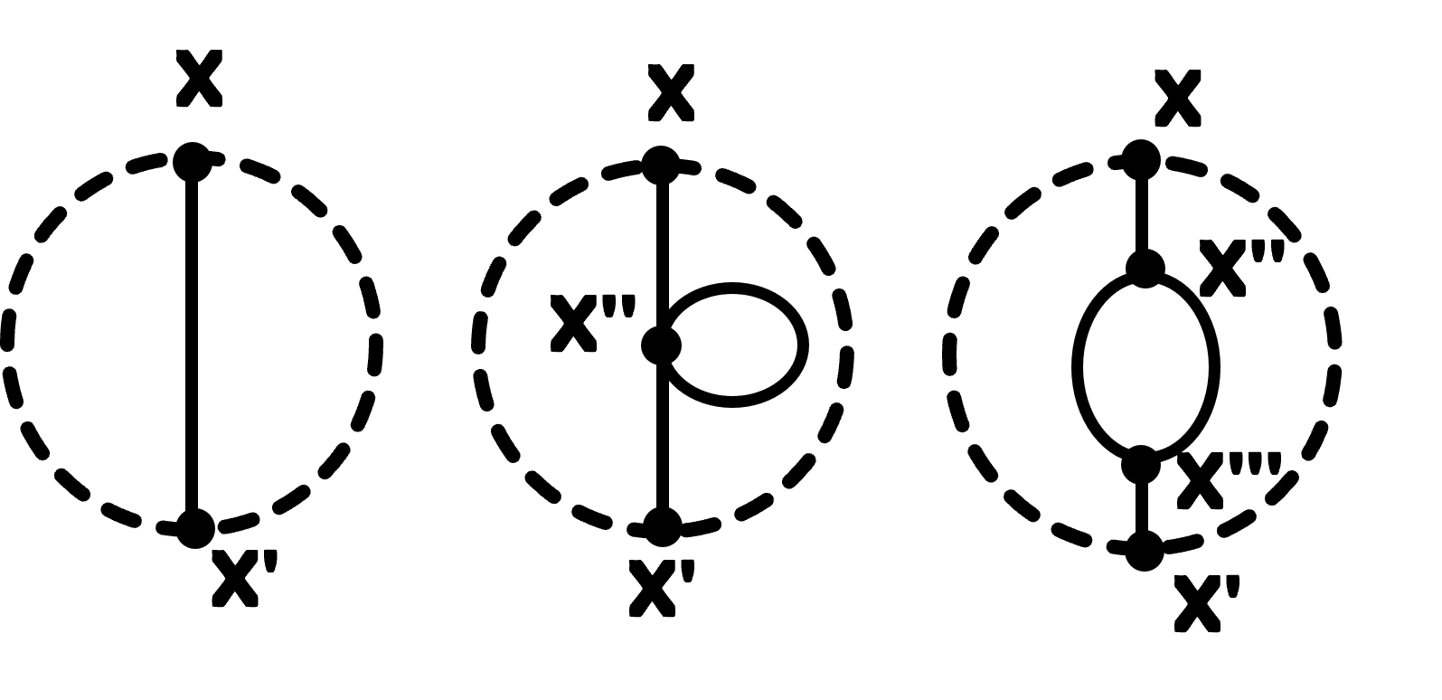
Figure 7: Vacuum diagrams for 64 up to three loop. Solid line denotes scalar whereas dashed line represents fermion. Primed vertices are integrated over. We have not included diagrams for $\langle\phi^{3}\rangle$ here, as it has already been computed earlier in 3.1 (2).

Let us first compute the leading secular contributions in 64. Majority of them are non-local. We first compute $\langle\phi^{4}\rangle$ as given by the first four diagrams of 7. At the lowest order, we have only the local contribution

$$\langle\phi^{4}(x)\rangle=3\langle\phi^{2}(x)\rangle^{2}=\frac{3H^{4}\ln^{2}a}{2^{4}\pi^{4}}$$ (65)

where in the last step we have used 115.

We now wish to compute ${\cal O}(\lambda)$ corrections to $\langle\phi^{4}(x)\rangle$. The connected bubble diagram (the second of 7) reads

$$\langle\phi^{4}(x)\rangle=-3i\lambda i\Delta(x,x)\times\int d^{4}x^{\prime}a^{\prime 4}i\Delta(x^{\prime},x^{\prime})\left(i\Delta_{++}^{2}(x,x^{\prime})-i\Delta_{+-}^{2}(x,x^{\prime})\right)$$ (66)

The leading contribution is non-local and corresponds to the causal part satisfying the temporal hierarchy, $\eta\gtrsim\eta^{\prime}$. Using the tools of spatial momentum space described in B, we find after a little algebra

$$\langle\phi^{4}(x)\rangle=\frac{3i\lambda H^{4}}{2^{4}\pi^{4}}\ln a\int d^{4}x^{\prime}a^{\prime 4}i\ln a^{\prime}\left(i\Delta_{+-}^{2}(x,x^{\prime})-i\Delta_{-+}^{2}(x,x^{\prime})\right)=-\frac{\lambda H^{4}}{2^{5}\times 3\pi^{6}}\ln^{4}a$$ (67)

The third diagram of 7 reads

$$\langle\phi^{4}(x)\rangle=-i\lambda\int d^{4}x^{\prime}a^{\prime 4}i\left(i\Delta_{++}^{4}(x,x^{\prime})-i\Delta_{+-}^{4}(x,x^{\prime})\right)$$ (68)

for which the leading secular part equals

$$\langle\phi^{4}(x)\rangle=i\lambda\int d^{4}x^{\prime}a^{\prime 4}\left(i\Delta_{+-}^{4}(x,x^{\prime})-i\Delta_{-+}^{4}(x,x^{\prime})\right)$$

$$=i\lambda\int d^{4}x^{\prime}a^{\prime 4}\left(i\Delta_{+-}^{2}(x,x^{\prime})+i\Delta_{-+}^{2}(x,x^{\prime})\right)\left(i\Delta_{+-}(x,x^{\prime})+i\Delta_{-+}(x,x^{\prime})\right)\left(i\Delta_{+-}(x,x^{\prime})-i\Delta_{-+}(x,x^{\prime})\right)=-\frac{\lambda H^{4}}{2^{6}\times 3\pi^{6}}\ln^{4}a$$

(69)

The fourth diagram of 7 contains correction due to the Yukawa interactions. Recalling that we are only interested in the contribution coming from the local part of the scalar self energy due to the fermion loop, the corresponding integral is written as

$$\langle\phi^{4}(x)\rangle=-12g^{2}i\Delta(x,x){\rm Tr}\int d^{4}x^{\prime}d^{4}x^{\prime\prime}(a^{\prime}a^{\prime\prime})^{4}\left(i\Delta_{++}(x,x^{\prime})i\Delta_{++}(x,x^{\prime\prime})iS^{2}_{++}(x^{\prime},x^{\prime\prime})+i\Delta_{+-}(x,x^{\prime})i\Delta_{+-}(x,x^{\prime\prime})iS^{2}_{--}(x^{\prime},x^{\prime\prime})\right)$$

(70)

The leading secular contribution for the above integral is given by

$$\frac{g^{2}H^{4}}{2^{3}\pi^{6}}\ln^{3}a$$ (71)

Combining now the above with 65, 67, 69 we have the perturbative result,

$$\langle\phi^{4}(x)\rangle=\frac{3H^{4}\ln^{2}a}{2^{4}\pi^{4}}-\frac{\lambda H^{4}}{2^{6}\pi^{6}}\ln^{4}a+\frac{g^{2}H^{4}}{2^{3}\pi^{6}}\ln^{3}a+\dots$$ (72)

4.2 Perturbative computation of $\langle\phi^{3}\rangle$

All the diagrams necessary to compute $\langle\phi^{3}\rangle$ up to three loop were considered in 3.1, given by 2 and 41.

4.3 Perturbative computation of $\langle\bar{\psi}\psi\phi\rangle$

We now wish to evaluate the last three diagrams of 7 for computing $\langle\bar{\psi}\psi\phi\rangle$. The leading order value of $\langle\bar{\psi}\psi\phi\rangle$ comes at ${\cal O}(g)$. Since we are only interested here in the local part of the square of the fermion propagator, it is clear that the diagram corresponding to this leading order (i.e., the third from the last of 7) will only contain purely local contributions, and hence we wish to discuss its renormalisation here. Using 18, the corresponding integral for $g\langle\bar{\psi}\psi\phi\rangle$ reads

$$-ig^{2}{\rm Tr}\int a^{\prime d}d^{d}x^{\prime}i\Delta_{++}(x,x^{\prime})iS^{2}_{++}(x,x^{\prime})=-\frac{\mu^{-\epsilon}g^{2}\Gamma(1-\epsilon/2)}{2^{2}\pi^{2-\epsilon/2}\epsilon(1-\epsilon)}\int d^{d}x^{\prime}\frac{a^{\prime d}}{(aa^{\prime})^{3-\epsilon/2}}i\Delta_{++}(x,x^{\prime})\partial^{2}_{x^{\prime}}\delta^{d}(x-x^{\prime})$$

$$-\frac{\mu^{-\epsilon}g^{2}}{2^{3}\pi^{2}}\int d^{d}x^{\prime}\frac{a^{\prime d}}{(aa^{\prime})^{3}}\ln(aa^{\prime})i\Delta_{++}(x,x^{\prime})\partial^{2}_{x^{\prime}}\delta^{d}(x-x^{\prime})-\frac{3g^{2}\epsilon}{2^{5}\pi^{2}}\int d^{4}x^{\prime}\frac{a^{\prime}}{a^{3}}\ln^{2}(aa^{\prime})i\Delta_{++}(x,x^{\prime})\partial^{2}_{x^{\prime}}\delta^{4}(x-x^{\prime})$$

(73)

We now consider the scalar field strength renormalisation counterterm (20) contribution, by making the replacement

$$-g^{2}{\rm Tr}\,iS^{2}(x,x^{\prime})\to\frac{ia^{d}\delta Z}{a^{2}(aa^{\prime})^{d}}$$

This cancels the first term on the right hand side of 73, and it gives after integrating by parts

$$\frac{\mu^{-\epsilon}g^{2}\Gamma(2-\epsilon)H^{4-\epsilon}}{2^{3-\epsilon}\pi^{4-\epsilon/2}\Gamma(1-\epsilon/2)\epsilon}\ln a+\frac{3g^{2}H^{4}}{2^{4}\pi^{4}}\ln^{2}a$$ (74)

In order to renormalise the above contribution, we further add the vacuum expectation value of a conformal counterterm,

$$\frac{1}{2}\delta\zeta R\langle\phi^{2}(x)\rangle=\frac{\delta\zeta RH^{2-\epsilon}\Gamma(2-\epsilon)}{2^{3-\epsilon}\pi^{2-\epsilon/2}\Gamma(1-\epsilon/2)}\left(\frac{1}{\epsilon}+\ln a\right)$$ (75)

where we have used 12. Hence the choice

$$\delta\zeta R=-\frac{\mu^{-\epsilon}g^{2}H^{2}}{\pi^{2}\epsilon}$$ (76)

simply cancels the first term of 74. The remaining divergence is constant and hence can be absorbed in a cosmological constant counterterm,

$$\frac{\delta\Lambda}{8\pi G}=\frac{\mu^{-\epsilon}g^{2}H^{4-\epsilon}\Gamma(2-\epsilon)}{2^{3-\epsilon}\pi^{4-\epsilon/2}\Gamma(1-\epsilon/2)\epsilon^{2}}$$ (77)

Thus the renormalised contribution for 73 equals

$$\frac{3g^{2}H^{4}}{2^{4}\pi^{4}}\ln^{2}a$$ (78)

We once again emphasise that the $\delta$-function appearing in 73 has basically converged all functions to the point $x$, asserting the term ‘local’.

The sixth and seventh diagrams of 7 contain both local and non-local contributions. Let us compute the leading or non-local terms first. The sixth diagram reads

$$-\frac{\lambda g}{2}{\rm Tr}\int d^{4}x^{\prime}d^{4}x^{\prime\prime}(a^{\prime}a^{\prime\prime})^{4}i\Delta(x^{\prime},x^{\prime})iS^{2}_{++}(x,x^{\prime\prime})\left(i\Delta_{++}(x,x^{\prime})i\Delta_{++}(x^{\prime\prime},x^{\prime})-i\Delta_{+-}(x,x^{\prime})i\Delta_{+-}(x^{\prime\prime},x^{\prime})\right)$$

$$=-\frac{i\lambda gH^{2}}{2^{5}\pi^{4}}\int d^{4}x^{\prime}a^{\prime 4}\ln a^{\prime}\partial_{x}^{2}\left(\frac{\ln a}{a^{2}}\left(i\Delta^{2}_{+-}(x,x^{\prime})-i\Delta^{2}_{-+}(x,x^{\prime})\right)\right)=-\frac{\lambda gH^{4}}{2^{5}\times 9\pi^{6}}\ln^{4}a$$ (79)

The seventh diagram of 7 reads,

$$ig\beta^{2}{\rm Tr}\int d^{4}x^{\prime}d^{4}x^{\prime\prime}d^{4}x^{\prime\prime\prime}(a^{\prime}a^{\prime\prime}a^{\prime\prime\prime})^{4}iS^{2}_{++}(x,x^{\prime\prime\prime})\left[i\Delta_{++}(x,x^{\prime})i\Delta_{++}(x^{\prime\prime\prime},x^{\prime\prime})i\Delta^{2}_{++}(x^{\prime},x^{\prime\prime})\right.$$

$$\left.-i\Delta_{++}(x,x^{\prime})i\Delta_{+-}(x^{\prime\prime\prime},x^{\prime\prime})i\Delta^{2}_{+-}(x^{\prime},x^{\prime\prime})-i\Delta_{+-}(x,x^{\prime})i\Delta_{++}(x^{\prime\prime\prime},x^{\prime\prime})i\Delta^{2}_{-+}(x^{\prime},x^{\prime\prime})\right.$$

$$\left.+i\Delta_{+-}(x,x^{\prime})i\Delta_{+-}(x^{\prime\prime\prime},x^{\prime\prime})i\Delta^{2}_{--}(x^{\prime},x^{\prime\prime})\right]$$ (80)

For $\eta\gtrsim\eta^{\prime}\gtrsim\eta^{\prime\prime}$, the above integral becomes

$$\frac{g\beta^{2}}{2^{2}\pi^{2}}\int d^{4}x^{\prime}d^{4}x^{\prime\prime}(a^{\prime}a^{\prime\prime})^{4}\partial_{x}^{2}\left[\frac{\ln a}{a^{2}}\left(i\Delta_{+-}(x,x^{\prime})-i\Delta_{-+}(x,x^{\prime})\right)\left(i\Delta_{+-}(x,x^{\prime\prime})i\Delta^{2}_{+-}(x^{\prime},x^{\prime\prime})-{\rm c.c.}\right)\right]$$

$$=\frac{g\beta^{2}}{2^{7}\times 9\pi^{6}}\ln^{5}a$$ (81)

whereas for the hierarchy $\eta\gtrsim\eta^{\prime\prime}\gtrsim\eta^{\prime}$, the contribution is exactly the same as above. Putting things together now, we have the perturbative result at the leading secular order,

$$\langle\bar{\psi}\psi\phi\rangle=\frac{3gH^{4}}{2^{4}\pi^{4}}\ln^{2}a-\frac{\lambda gH^{4}}{2^{5}\times 9\pi^{6}}\ln^{4}a+\frac{g\beta^{2}H^{2}}{2^{6}\times 9\pi^{6}}\ln^{5}a+\dots$$ (82)

Substituting the above along with 41, 72 into 64, we have the perturbative result

$$\frac{d\langle\bar{\phi}^{2}\rangle}{d{\cal N}}=\frac{1}{4\pi^{2}}-\left[\frac{\lambda{\cal N}^{2}}{2^{4}\times 3\pi^{4}}-\frac{\lambda^{2}{\cal N}^{4}}{2^{6}\times 9\pi^{6}}-\frac{7\bar{\beta}^{2}{\cal N}^{3}}{2^{6}\times 9\pi^{4}}+\frac{g^{2}{\cal N}^{2}}{2^{3}\pi^{4}}-\frac{\lambda g^{2}{\cal N}^{4}}{2^{4}\times 27\pi^{6}}+\frac{g^{2}\bar{\beta}^{2}{\cal N}^{5}}{2^{5}\times 27\pi^{6}}\right]$$ (83)

so that we have

$$\langle\bar{\phi}^{2}\rangle=\frac{{\cal N}}{4\pi^{2}}-\frac{\lambda{\cal N}^{3}}{2^{4}\times 9\pi^{4}}+\frac{\lambda^{2}{\cal N}^{5}}{2^{6}\times 45\pi^{6}}+\frac{7\bar{\beta}^{2}{\cal N}^{4}}{2^{6}\times 36\pi^{4}}-\frac{g^{2}{\cal N}^{3}}{2^{3}\times 3\pi^{4}}+\frac{\lambda g^{2}{\cal N}^{5}}{2^{4}\times 135\pi^{6}}-\frac{g^{2}\bar{\beta}^{2}{\cal N}^{6}}{2^{5}\times 162\pi^{6}}$$ (84)

where $\bar{\phi}=\phi/H$ and $\bar{\beta}=\beta/H$ are dimensionless as before. Promoting now 83 to non-perturbative level as earlier, we have

$$\frac{d\langle\bar{\phi}^{2}\rangle}{d{\cal N}}=\frac{1}{4\pi^{2}}-\frac{\lambda\langle\bar{\phi}^{2}\rangle^{2}}{3}+\frac{4\pi^{2}\lambda^{2}\langle\bar{\phi}^{2}\rangle^{4}}{27}-\frac{80\pi^{2}\lambda g^{2}\langle\bar{\phi}^{2}\rangle^{4}}{27}+\frac{7\pi^{2}\bar{\beta}^{2}\langle\bar{\phi}^{2}\rangle^{3}}{9}-2g^{2}\langle\bar{\phi}^{2}\rangle^{2}+\frac{52\pi^{4}g^{2}\bar{\beta}^{2}\langle\bar{\phi}^{2}\rangle^{5}}{27}$$ (85)

The solution to the above equation turns out to be complex for certain values in the parameter space. This is unacceptable, since $\phi(x)$ is hermitian and hence $\langle\phi^{2}\rangle$ must be a real, positive definite quantity. It can be readily verified that the above equation can be integrated only if we ignore the cubic coupling term. In that case we have for large ${\cal N}$,

$$\langle\bar{\phi}^{2}\rangle=\frac{3\sqrt{6g^{2}+\lambda}}{4\pi g\sqrt{10\lambda}}\left[-1+\left(1+\frac{80\lambda g^{2}}{3(6g^{2}+\lambda)^{2}}\right)^{1/2}\right]^{\frac{1}{2}}$$

However, if we understand it correctly, the above result seems to be a bit misleading! This is because we have not attempted to distinguish between the purely local and non-local terms in 85. Let us now consider the purely non-local terms

$$\frac{d\langle\bar{\phi}^{2}\rangle_{\rm NL}}{d{\cal N}}=\frac{4\pi^{2}\lambda^{2}\langle\bar{\phi}^{2}\rangle^{4}_{\rm NL}}{27}-\frac{80\pi^{2}\lambda g^{2}\langle\bar{\phi}^{2}\rangle^{4}_{\rm NL}}{27}+\frac{7\pi^{2}\bar{\beta}^{2}\langle\bar{\phi}^{2}\rangle^{3}_{\rm NL}}{9}+\frac{52\pi^{4}g^{2}\bar{\beta}^{2}\langle\bar{\phi}^{2}\rangle^{5}_{\rm NL}}{27}$$ (86)

which gives

$$\int\frac{d\langle\bar{\phi}^{2}\rangle_{\rm NL}}{\langle\bar{\phi}^{2}\rangle^{3}_{\rm NL}\left[7\bar{\beta}^{2}+\frac{4\lambda}{3}\left(\lambda-20g^{2}\right)\langle\bar{\phi}^{2}\rangle_{\rm NL}+\frac{52\pi^{2}g^{2}\bar{\beta}^{2}}{3}\langle\bar{\phi}^{2}\rangle_{\rm NL}^{2}\right]}=\frac{\pi^{2}{\cal N}}{9}$$ (87)

It is easy to check that the quadratic cannot have real and positive roots for all values of the couplings. Could it possibly indicate that $\langle\bar{\phi}^{2}\rangle_{\rm NL}$ is vanishing? Even though we shall not investigate the asymptotic behaviour of $\langle\bar{\phi}^{2}\rangle_{\rm NL}$ explicitly in this paper, we wish to comment a little bit more on this issue towards the end of the following section, and will argue that possibly a more careful analysis is necessary to predict anything specific about the same. We also note in this context that for a quartic self interaction, it was argued in [47] using the Schwinger-Dyson equation for the Feynman propagator that the same can admit one asymptotically vanishing non-perturbative solution. See also the discussion of [50] on resummed two point correlation function for quartic self interaction beyond local approximation.

4.4 The purely local contribution and the dynamical mass

Let us now consider the purely local contributions to $\langle\phi^{2}(x)\rangle$. The renormalised $\langle\phi^{2}(x)\rangle$ containing contributions only from the local part of the self energy at ${\cal O}(\lambda)$, ${\cal O}(\lambda^{2})$ and ${\cal O}(\beta^{2})$ for one particle irreducible (1PI) diagrams are given by [53],

$$\langle\phi^{2}(x)\rangle_{\rm loc.,Ren.}=-\frac{\lambda H^{2}{\cal N}^{3}}{2^{4}\times 9\pi^{4}}+\frac{\beta^{2}{\cal N}^{3}}{2^{5}\times 9\pi^{4}}+\frac{\lambda^{2}H^{2}{\cal N}^{4}}{2^{9}\times 3\pi^{6}}$$ (88)

Let us now consider the local contribution due to ${\cal O}(g^{2})$ loop correction to the $\lambda\phi^{4}$ term in 64. It reads

$$\frac{i\lambda g^{2}}{2^{2}}i\Delta(x,x){\rm Tr}\int d^{d}x^{\prime}d^{d}x^{\prime\prime}(a^{\prime}a^{\prime\prime})^{d}iS^{2}_{++}(x^{\prime},x^{\prime\prime})i\Delta_{++}(x,x^{\prime})i\Delta_{++}(x,x^{\prime\prime})$$

$$=\frac{\mu^{-\epsilon}\lambda g^{2}\Gamma(1-\epsilon/2)}{2^{4}\pi^{2-\epsilon/2}\epsilon(1-\epsilon)}i\Delta(x,x)\int d^{d}x^{\prime}d^{d}x^{\prime\prime}\frac{(a^{\prime}a^{\prime\prime})^{d}}{(a^{\prime}a^{\prime\prime})^{3-\epsilon}}(\partial_{x^{\prime\prime}}^{2}\delta^{d}(x^{\prime}-x^{\prime\prime}))i\Delta_{++}(x,x^{\prime})i\Delta_{++}(x,x^{\prime\prime})$$

$$=\frac{\mu^{-\epsilon}\lambda g^{2}\Gamma(1-\epsilon/2)}{2^{4}\pi^{2-\epsilon/2}\epsilon(1-\epsilon)}i\Delta(x,x)\int d^{d}x^{\prime}\partial_{x^{\prime}}^{2}\left(a^{\prime 2}i\Delta^{2}_{++}(x,x^{\prime})\right)$$ (89)

where we have used 18. Now, the local part of $i\Delta^{2}_{++}(x,x^{\prime})$ contains a $\delta$-function, 86. The integral $\partial_{x^{\prime}}^{2}\left(a^{\prime 2}i\Delta^{2}_{++}(x,x^{\prime})\right)$ can be converted to a boundary integral making it vanishing. Similarly the ${\cal O}(\beta g^{2})$ local correction to the cubic potential term also vanishes. This happens due to the fact that the scalar self energy due to fermion loop is accompanied by a $\partial^{2}$. However, there is certainly non-vanishing non-local contributions, as evaluated in 70, 71.

Let us now consider the Yukawa term $g\langle\bar{\psi}\psi\phi\rangle$ in 64. Its leading local and renormalised expression was computed in the preceding section, given by 78.

We now wish to compute the local contributions at ${\cal O}(\lambda g^{2})$ and ${\cal O}(\beta^{2}g^{2})$ for the same, where one Yukawa interaction term sits at the unintegrated vertex, $x$ (the last two diagrams of 7). We shall see that these local contributions are non-vanishing unlike the above. We have at ${\cal O}(\lambda g^{2})$,

$$-\frac{\lambda g^{2}}{2}{\rm Tr}\int d^{d}x^{\prime}d^{d}x^{\prime\prime}(a^{\prime}a^{\prime\prime})^{d}iS^{2}_{++}(x,x^{\prime})i\Delta_{++}(x,x^{\prime\prime})i\Delta_{++}(x^{\prime},x^{\prime\prime})i\Delta(x^{\prime\prime},x^{\prime\prime})$$

$$=-\frac{\lambda g^{2}H^{2-\epsilon}\Gamma(2-\epsilon)}{2^{3-\epsilon}\pi^{2-\epsilon/2}\Gamma(1-\epsilon/2)}{\rm Tr}\int d^{d}x^{\prime}d^{d}x^{\prime\prime}(a^{\prime}a^{\prime\prime})^{d}iS^{2}_{++}(x,x^{\prime})i\Delta_{++}(x,x^{\prime\prime})i\Delta_{++}(x^{\prime},x^{\prime\prime})\left(\frac{1}{\epsilon}+\ln a^{\prime\prime}\right)$$ (90)

We add to the above the contribution coming from the one loop mass renormalisation counterterm due to quartic self interaction, $\delta m^{2}_{\lambda}$ given by 13,

$$-g^{2}\delta m_{\lambda}^{2}{\rm Tr}\int(a^{\prime}a^{\prime\prime})^{d}d^{d}x^{\prime}d^{d}x^{\prime\prime}iS_{++}^{2}(x,x^{\prime})i\Delta_{++}(x,x^{\prime\prime})i\Delta_{++}(x^{\prime},x^{\prime\prime})$$

$$=\frac{\lambda H^{2-\epsilon}\Gamma(2-\epsilon)}{2^{3-\epsilon}\pi^{2-\epsilon/2}\Gamma(1-\epsilon/2)\epsilon}{\rm Tr}\int(a^{\prime}a^{\prime\prime})^{d}d^{d}x^{\prime}d^{d}x^{\prime\prime}iS_{++}^{2}(x,x^{\prime})i\Delta_{++}(x,x^{\prime\prime})i\Delta_{++}(x^{\prime},x^{\prime\prime})$$ (91)

so that after using 18 for the square of the fermion propagator, the above equation becomes

$$\frac{i\mu^{-\epsilon}\lambda g^{2}H^{2-\epsilon}\Gamma(1-\epsilon)}{2^{5-\epsilon}\pi^{4-\epsilon}\epsilon}\int d^{d}x^{\prime}d^{d}x^{\prime\prime}\frac{(a^{\prime}a^{\prime\prime})^{d}}{(aa^{\prime})^{3-\epsilon/2}}(\partial^{2}_{x^{\prime}}\delta^{d}(x-x^{\prime}))i\Delta_{++}(x,x^{\prime\prime})i\Delta_{++}(x^{\prime},x^{\prime\prime})\ln a^{\prime\prime}$$

$$+\frac{i\mu^{-\epsilon}\lambda g^{2}H^{2-\epsilon}\Gamma(2-\epsilon)}{2^{6-\epsilon}\pi^{4-\epsilon/2}\Gamma(1-\epsilon/2)}\int d^{d}x^{\prime}d^{d}x^{\prime\prime}\frac{(a^{\prime}a^{\prime\prime})^{d}}{(aa^{\prime})^{3}}\ln(aa^{\prime})(\partial^{2}_{x^{\prime}}\delta^{d}(x-x^{\prime}))i\Delta_{++}(x,x^{\prime\prime})i\Delta_{++}(x^{\prime},x^{\prime\prime})\ln a^{\prime\prime}$$

$$+\frac{3i\epsilon\mu^{-\epsilon}\lambda g^{2}H^{2-\epsilon}\Gamma(2-\epsilon)}{2^{8-\epsilon}\pi^{4-\epsilon/2}\Gamma(1-\epsilon/2)}\int d^{d}x^{\prime}d^{d}x^{\prime\prime}\frac{(a^{\prime}a^{\prime\prime})^{d}}{(aa^{\prime})^{3}}\ln^{2}(aa^{\prime})(\partial^{2}_{x^{\prime}}\delta^{d}(x-x^{\prime}))i\Delta_{++}(x,x^{\prime\prime})i\Delta_{++}(x^{\prime},x^{\prime\prime})\ln a^{\prime\prime}$$ (92)

Let us consider the first integral above. It can as earlier be canceled by the scalar field strength renormalisation counterterm, 20. The second integral turns out to be completely ultraviolet divergent

$$-\frac{\mu^{-2\epsilon}\lambda g^{2}H^{4-\epsilon}\Gamma(1-\epsilon)}{2^{7-\epsilon}\pi^{6-\epsilon}}\frac{\ln^{2}a}{\epsilon}$$ (93)

whereas the third integral pf 92 is completely ultraviolet finite,

$$-\frac{3\lambda g^{2}H^{4}}{2^{8}\pi^{6}}\ln^{3}a$$ (94)

Thus we identify the ultraviolet divergent and finite parts of 92 as

$$-\frac{\mu^{-2\epsilon}\lambda g^{2}H^{4-\epsilon}\Gamma(1-\epsilon)}{2^{7-\epsilon}\pi^{6-\epsilon}}\frac{\ln^{2}a}{\epsilon}-\frac{3\lambda g^{2}H^{4}}{2^{8}\pi^{6}}\ln^{3}a$$ (95)

In order to renormalise the above expression, we add with it the ${\cal O}(\lambda)$ corrections to the conformal counterterm introduced in 76. These corrections respectively correspond to the quartic self interaction and the one loop mass counterterm corresponding to the quartic self interaction. They read

$$-\frac{i\lambda\delta\zeta R}{2^{2}}\int d^{d}x^{\prime}a^{\prime d}i\Delta_{++}^{2}(x,x^{\prime})i\Delta(x^{\prime},x^{\prime})-\frac{i\delta\zeta R\,\delta m_{\lambda}^{2}}{2}\int d^{d}x^{\prime}a^{\prime d}i\Delta^{2}_{++}(x,x^{\prime})$$

$$=\frac{\mu^{-2\epsilon}\lambda g^{2}H^{4-\epsilon}\Gamma(1-\epsilon)}{2^{7-\epsilon}\pi^{6-\epsilon}}\left(\frac{1}{\epsilon^{3}}+\frac{2\ln a}{\epsilon^{2}}+\frac{3\ln^{2}a}{2\epsilon}+\frac{2}{3}\ln^{3}a\right)-\frac{\mu^{-2\epsilon}\lambda g^{2}H^{4-\epsilon}\Gamma(1-\epsilon)}{2^{7-\epsilon}\pi^{6-\epsilon}}\left(\frac{1}{\epsilon^{3}}+\frac{\ln a}{\epsilon^{2}}+\frac{\ln^{2}a}{2\epsilon}+\frac{1}{6}\ln^{3}a\right)$$

$$=\frac{\mu^{-2\epsilon}\lambda g^{2}H^{4-\epsilon}\Gamma(1-\epsilon)}{2^{7-\epsilon}\pi^{6-\epsilon}}\left(\frac{\ln a}{\epsilon^{2}}+\frac{\ln^{2}a}{\epsilon}\right)+\frac{\lambda g^{2}H^{4}}{2^{7}\pi^{6}}\ln^{3}a$$ (96)

The above expression, when combined with 95, cancels the ultraviolet divergence for the $\ln^{2}a$ term. The remaining logarithmic divergence can be canceled as earlier by a conformal counterterm of ${\cal O}(\lambda g^{2})$, leaving us with the renormalised expression for the integral 90,

$$-\frac{\lambda g^{2}H^{4}}{2^{8}\pi^{6}}\ln^{3}a$$ (97)

The diagram at ${\cal O}(\beta^{2}g^{2})$ can be computed in a similar manner. It reads

$$\frac{i\beta^{2}g^{2}}{2}{\rm Tr}\int d^{d}x^{\prime}d^{d}x^{\prime\prime}d^{d}x^{\prime\prime\prime}(a^{\prime}a^{\prime\prime}a^{\prime\prime\prime})^{d}iS^{2}_{++}(x,x^{\prime})i\Delta_{++}(x,x^{\prime\prime})i\Delta_{++}(x^{\prime},x^{\prime\prime\prime})i\Delta^{2}_{++}(x^{\prime\prime},x^{\prime\prime\prime})$$

$$=\frac{\mu^{-\epsilon}\beta^{2}g^{2}\Gamma(1-\epsilon/2)}{2^{4}\pi^{2-\epsilon/2}\epsilon(1-\epsilon)}{\rm Tr}\int d^{d}x^{\prime}d^{d}x^{\prime\prime}(a^{\prime}a^{\prime\prime})^{d}iS^{2}_{++}(x,x^{\prime})i\Delta_{++}(x,x^{\prime\prime})i\Delta_{++}(x^{\prime},x^{\prime\prime})\left(1+\epsilon\ln a^{\prime\prime}+\frac{\epsilon^{2}}{2}\ln^{2}a^{\prime\prime}+{\cal O}(\epsilon^{3})\right)$$

(98)

We add with it the one loop mass renormalisation counterterm contribution due to the cubic self interaction, 15, to have

$$-\delta m_{\beta}^{2}g^{2}{\rm Tr}\int d^{d}x^{\prime}d^{d}x^{\prime\prime}(a^{\prime}a^{\prime\prime})^{d}iS^{2}_{++}(x,x^{\prime})i\Delta_{++}(x,x^{\prime\prime})i\Delta_{++}(x^{\prime},x^{\prime\prime})$$ (99)

which cancels the first divergence (i.e., the first term) of 98. We now have

$$-\frac{i\mu^{-2\epsilon}\beta^{2}g^{2}\Gamma^{2}(1-\epsilon/2)}{2^{6}\pi^{4-\epsilon}\epsilon(1-\epsilon)^{2}}\int d^{d}x^{\prime\prime}\partial_{x}^{2}\left(\frac{(aa^{\prime\prime})^{d}}{a^{6-\epsilon}}i\Delta^{2}_{++}(x,x^{\prime\prime})f(a^{\prime\prime})\right)$$

$$-\frac{i\mu^{-2\epsilon}\beta^{2}g^{2}\Gamma(1-\epsilon/2)}{2^{6}\pi^{4-\epsilon/2}(1-\epsilon)}\int d^{d}x^{\prime\prime}\partial_{x}^{2}\left(\frac{(aa^{\prime\prime})^{d}}{a^{6}}\ln a\,i\Delta^{2}_{++}(x,x^{\prime\prime})f(a^{\prime\prime})\right)$$

$$-\frac{3i\epsilon\mu^{-2\epsilon}\beta^{2}g^{2}\Gamma(1-\epsilon/2)}{2^{7}\pi^{4-\epsilon/2}(1-\epsilon)}\int d^{d}x^{\prime\prime}\partial_{x}^{2}\left(\frac{(aa^{\prime\prime})^{d}}{a^{6}}\ln^{2}a\,i\Delta^{2}_{++}(x,x^{\prime\prime})f(a^{\prime\prime})\right)$$ (100)

where we have abbreviated for the sake of convenience

$$f(a)=\ln a+\frac{\epsilon}{2}\ln^{2}a$$

The first line of the above equation can as earlier be canceled by the scalar field strength renormalisation counterterm’s contribution. The remaining integrals give

$$\frac{\mu^{-3\epsilon}\beta^{2}g^{2}H^{2}\Gamma^{2}(1-\epsilon/2)}{2^{8}\pi^{6-\epsilon}(1-\epsilon)^{2}}\left(\frac{\ln^{2}a}{\epsilon}+\frac{1}{2}\ln^{3}a\right)+\frac{3\beta^{2}H^{2}g^{2}}{2^{9}\pi^{6}}\ln^{3}a$$ (101)

We consider the ${\cal O}(\beta^{2})$ correction to the conformal counterterm, 76,

$$-\frac{\delta\zeta\beta^{2}R}{2^{2}}\int d^{d}x^{\prime}d^{d}x^{\prime\prime}(a^{\prime}a^{\prime\prime})^{d}i\Delta_{++}(x,x^{\prime})i\Delta_{++}(x,x^{\prime\prime})i\Delta^{2}_{++}(x^{\prime},x^{\prime\prime})-\frac{\delta\zeta R\delta m^{2}_{\beta}}{2}\int d^{d}x^{\prime}a^{\prime d}i\Delta^{2}_{++}(x,x^{\prime})$$

$$=-\frac{\mu^{-3\epsilon}\beta^{2}g^{2}H^{2}\Gamma^{2}(1-\epsilon/2)}{2^{8}\pi^{6-\epsilon}(1-\epsilon)^{2}}\left(\frac{1}{\epsilon^{3}}+\frac{2\ln a}{\epsilon^{2}}+\frac{2\ln^{2}a}{\epsilon}+\frac{4}{3}\ln^{3}a\right)+\frac{\mu^{-3\epsilon}\beta^{2}g^{2}H^{2}\Gamma^{2}(1-\epsilon/2)}{2^{8}\pi^{6-\epsilon}(1-\epsilon)^{2}}\left(\frac{1}{\epsilon^{3}}+\frac{\ln a}{\epsilon^{2}}+\frac{\ln^{2}a}{2\epsilon}+\frac{1}{6}\ln^{3}a\right)$$

(102)

The above, when combined with 101, yields

$$\frac{\mu^{-3\epsilon}\beta^{2}g^{2}H^{2}\Gamma^{2}(1-\epsilon/2)}{2^{8}\pi^{6-\epsilon}(1-\epsilon)^{2}}\left(-\frac{\ln a}{\epsilon^{2}}-\frac{\ln^{2}a}{2\epsilon}\right)+\frac{5\beta^{2}H^{2}g^{2}}{2^{9}\times 3\pi^{6}}\ln^{3}a$$ (103)

Now, the logarithmic divergence appearing above can be absorbed by an ${\cal O}(\beta^{2}g^{2})$ conformal counterterm as earlier. However unlike the quartic self interaction, the $\ln^{2}a$ remains. Probably we need to consider terms where both local and non-local terms coincide and the divergence due to the local term cancels the same. We shall not further pursue it here and instead proceed with the finite term appearing in 103. Combining this with 78, 88 and 97, we have from 64 for the local contributions

$$\frac{d\langle\bar{\phi}^{2}\rangle_{\rm loc}}{d{\cal N}}=\frac{1}{4\pi^{2}}-\left(g^{2}+\frac{\lambda}{6}-\frac{\bar{\beta}^{2}}{12}\right)\frac{{\cal N}^{2}}{2^{3}\pi^{4}}+\left(\lambda^{2}+\lambda g^{2}-\frac{5\bar{\beta}^{2}g^{2}}{6}\right)\frac{{\cal N}^{3}}{2^{7}\times 3\pi^{6}}$$ (104)

which reads when promoted to non-perturbative level

$$\frac{d\langle\bar{\phi}^{2}\rangle_{\rm loc}}{d{\cal N}}=\frac{1}{4\pi^{2}}-2\left(g^{2}+\frac{\lambda}{6}-\frac{\bar{\beta}^{2}}{12}\right)\langle\bar{\phi}^{2}\rangle^{2}_{\rm loc}+\frac{1}{6}\left(\lambda^{2}+\lambda g^{2}-\frac{5\bar{\beta}^{2}g^{2}}{6}\right)\langle\bar{\phi}^{2}\rangle^{3}_{\rm loc}$$ (105)

However, the above integration gives complex $\langle\bar{\phi}^{2}\rangle_{\rm loc}$ for certain parameter values, which is once again unacceptable. We can encounter this issue as follows. Note that here we are dealing with the diagrams of 7 in order to compute the first derivative of $\langle\bar{\phi}^{2}\rangle$. Naturally, as we have also discussed below 58 in the context of tadpoles, while integrating this expression we basically introduce an external point on each of these diagrams where two scalar propagators meet. Consequently, the original unintegrated vertex at $x$ now becomes a dummy vertex. This gives us the vacuum expectation value of the scalar two point function in the coincidence limit.

As has been done in C for $\langle\phi\rangle$, let us now perform an explicit computation for $\langle\phi^{2}\rangle$ by considering e.g. the first of 7. When its contribution is integrated with respect to the $e$-foldings, we obtain the second term on the right hand side of 84. As we have stated above, at the diagrammatic level for $\langle\phi^{2}\rangle$, this should be equivalent to introducing an external point $x$ on any of the loops of the first of 7, and subsequently to replace the original vertex at $x$ by a dummy one, say $x^{\prime}$, giving us the ${\cal O}(\lambda)$ contribution,

$$\langle\phi^{2}(x)\rangle=-\frac{i\lambda}{2}\int d^{4}xa^{4}i\Delta(x^{\prime},x^{\prime})\left[i\Delta^{2}_{++}(x,x^{\prime})-i\Delta^{2}_{+-}(x,x^{\prime})\right]$$

It can be easily checked that (e.g. [53]) the above exactly matches with the aforementioned result of 84. Now, since these diagrams for the two point correlator will contain self energy loops, we should take the 1PI diagrams only. However, it is easy to see that there is no such 1PI diagrams corresponding to the last to diagrams of 7. This is because the corresponding integrated version of these two diagrams will contain the external point between $x^{\prime\prime}$ and the initial unintegrated vertex at $x$. Hence it seems reasonable to discard them. Note that we do not need to worry about similar things while computing the scalar one point function, for any diagram corresponding to $\langle\phi\rangle$ contains tadpole (connected to an external point) which cannot be 1PI. Indeed, after ignoring the ${\cal O}(\lambda g^{2})$, ${\cal O}(\beta^{2}g^{2})$ terms in 105, we find a real and positive result for $\langle\bar{\phi}^{2}\rangle_{\rm loc}$, as depicted in 8 and 9.

A finite and non-vanishing $\langle\bar{\phi}^{2}\rangle_{\rm loc}$ also indicates mass for the scalar field, dictated by the formula [80, 81]

$$\frac{m^{2}_{\rm dyn}}{H^{2}}=\frac{3}{8\pi^{2}\langle\bar{\phi}^{2}\rangle_{\rm loc}}$$ (106)

which is depicted in 10. Since the scalar field was massless initially, this mass has generated dynamically. Since a massive scalar, no matter how tiny its mass is, obeys the de Sitter invariance, the dynamical mass generation clearly shows that the secular effect cannot eventually destroy the de Sitter spacetime. However, the backreaction due to the matter field might change the inflationary $\Lambda$ value. We refer our reader for earlier discussion on dynamical mass generation in de Sitter spacetime for a self interacting scalar field [41, 47, 50, 51, 53], and also to [54] in the context of scalar quantum electrodynamics.

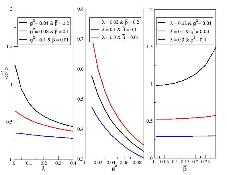
Figure 8: The variation of $\langle\bar{\phi}^{2}\rangle_{\rm loc}$ with respect to different couplings. See main text for discussion.

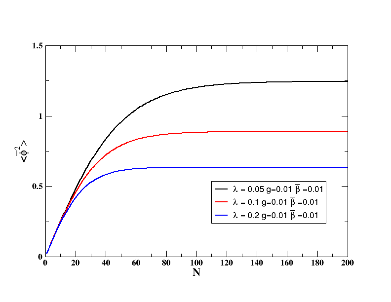
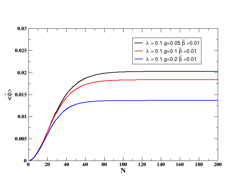
Figure 9: The variation of $\langle\bar{\phi}^{2}\rangle_{\rm loc}$ with respect to the number of $e$-foldings, ${\cal N}$. See main text for discussion.

Figure 10: The variation of the dynamical mass, 106, of the scalar field with respect to different couplings. The decrease in $m^{2}_{\rm dyn}/H^{2}$ with the cubic coupling certainly corresponds to the destabilising effect of the cubic scalar potential.

Before we end, we wish to comment on $\langle\phi^{2}\rangle_{\rm NL}$ mentioned in the previous section. First note that if we accept that we should consider diagrams which only generate 1PI self energy contributions for the scalar two point correlation function, we should further exclude from 85 all such non-desired terms, for example from the group 2. Next, since the scalar has dynamically become massive now, it seems natural that we should incorporate the same into 85, in order to get the correct physics. For the mass term only, $\langle\phi^{2}\rangle$ falls off as $e^{-m^{2}_{\rm dyn}{\cal N}/H^{2}}$. Thus as the simplest approximation, one may wish to treat the non-local terms in 85 as sources and can substitute $\langle\phi^{2}\rangle\sim e^{-m^{2}_{\rm dyn}{\cal N}/H^{2}}$ there, giving $\langle\phi^{2}\rangle_{\rm NL}\to 0$ at late times. However to the best of our understanding, in order to draw any clear conclusion on $\langle\phi^{2}\rangle_{\rm NL}$, it seems that we need a more careful and rigourous analysis regarding the 1PI non-local part of the self energy. Specifically, along with the dynamically generated scalar mass, we should also consider resumming those self energy constributions, instead of making the aforementioned substition of $e^{-m^{2}_{\rm dyn}{\cal N}/H^{2}}$ in place of them. Perhaps we might even need to go to higher order loop computations. This seems to be a non-trivial and technically non-trivial task compared to that of the pure local contributions, and we wish to come back to this issue in a future work.

5 Discussion

In this work we have considered the secular effect for a massless and minimal quantum scalar field with an asymmetric self interaction (1) coupled to massless fermion via the Yukawa interaction, 7, in the inflationary de Sitter background. We note that this potential has shape wise similarity with the standard slow roll inflationary ones. The scalar is initially assumed to be located around the flat region $(\phi\sim 0)$ of the potential, so that perturbation theory with respect to the Bunch-Davies vacuum holds good initially. As time goes on, the system should roll down towards the minima of the potential. However in the due course of this rolling, there will be strong quantum effects, dictated by the secular logarithms, originating from the highly stretched, super-Hubble late time modes. We have considered the late time large wavelength equation of motion for the scalar field, and have constructed the first order differential equations satisfied by $\langle\phi\rangle$ and $\langle\phi^{2}\rangle$ (with respect to the initial Bunch-Davies vacuum), respectively 22, 64. These equations are sourced by vacuum expectation values of various combinations of the field operators. We have computed these vacuum expectation values up to three loop, in terms of the leading secular logarithms. Using these perturbative results, we have constructed next the non-perturbative equations of motion for $\langle\phi\rangle$ and $\langle\phi^{2}\rangle$ and have found out their non-perturbative values respectively in 3 and 4. 62 shows that the magnitude $\langle\phi\rangle$ decreases with increasing Yukawa coupling. We also note that the resulting $\langle\phi\rangle$ is not close to $-3\beta/\lambda$ i.e., the point of classical minimum of the potential, clearly revealing the strong quantum effect. On the other hand, a finite and non-vanishing $\langle\phi^{2}\rangle$ in particular, indicates a dynamically generated mass of the scalar field, 106, which has been investigated in the preceding section. On the other hand, a detailed and systematic analysis for the resummed $\langle\phi^{2}\rangle$ containing the effect of the non-local self-energy as well as the dynamical mass will be reported in a future work (cf., discussion at the end of the preceding section).

We have seen that if we consider all the diagrams for the computation of $\langle\phi^{2}\rangle$, we may obtain complex values for certain parameter ranges (cf., discussion below 105), which is certainly unacceptable for $\phi$ is hermitian. As we have argued, since the diagrams correspond to the derivative of $\langle\phi^{2}\rangle$, and the subsequent integration basically inserts an external point on a scalar line in any diagram, we should first check whether any diagram, after such insertion, yields an 1PI contribution. This not only rules out the non-1PI diagrams for example from the group 2, but also the last two diagrams of 7 which are 1PI to begin with. Note for these two latter diagrammes that the external points after integration are to be inserted between $x$ and $x^{\prime\prime}$, and the original vertices at $x$ becomes dummy. Accordingly, the two resulting diagrams are not 1PI. Perhaps one should keep in mind this algorithm while resumming the scalar two point function. We also note that we did not encounter any such problem while computing $\langle\phi\rangle$, for if we integrate any diagram corresponding to its derivative, we basically generate a non-amputated tadpole, 11. Clearly such diagram cannot be 1PI (cf., the discussion below 105).

It seems to be an important task to compute a non-perturbative vacuum expectation values of the interaction potential and the scalar self interaction potential. Finding out a non-perturbative effective potential seems to be an interesting task too. We wish to come back to these issues in our future publications.

Appendix A The in-in formalism

The standard quantum field theory involves computing $S$-matrix elements of observables with respect to in and out states while the vacuum of the theory is uniquely defined and stable. For a dynamical background such as the de Sitter however, the initial vacuum state is not stable and decays into a final one due to particle pair creation. Apart from this we also note that the interactions cannot be adiabatically turned on and off in a cosmological scenario and in fact they are present all the way throughout. Moreover unlike the flat spacetime, we do not have a freedom to define our initial and final states respectively at temporal past and future infinities. In such backgrounds, one needs the Schwinger-Keldysh or the in-in or the closed time path formalism to compute the expectation value of any operator meaningfully, which we wish to review very briefly below, referring our reader to [82, 83, 84, 85, 86] and references therein for excellent pedagogical detail.

The functional integral representation of the standard in-out matrix elements with respect to the field basis reads

$$\langle\phi|T(O_{1}[\phi])|\psi\rangle=\int\mathcal{D}\phi\,e^{i\int_{t_{i}}^{t_{f}}\sqrt{-g}d^{d}x\mathcal{L}[\phi]}\Phi^{\star}\left[\phi\left(t_{f}\right)\right]O_{1}[\phi]\Psi\left[\phi\left(t_{i}\right)\right]$$ (107)

where $T$ stands for time ordering, $O_{1}[\phi]$ is some observable and $\Phi$, $\Psi$ are the wave functionals with respect to the field kets $|\phi\rangle$ and $|\psi\rangle$ respectively. We also have the representation for anti-time ordering as

$$\langle\psi|\bar{T}(O_{2}([\phi]))|\phi\rangle=\int\mathcal{D}\phi e^{-i\int_{t_{i}}^{t_{f}}\sqrt{-g}d^{d}x\mathcal{L}[\phi]}\Phi\left[\phi\left(t_{i}\right)\right]O_{2}[\phi]\Psi^{\star}\left[\phi\left(t_{f}\right)\right]$$ (108)

Combining the above with 107, we write down the in-in matrix representation

$$\langle\psi|\bar{T}(O_{2}[\phi])T(O_{1}[\phi])|\psi\rangle=\int\mathcal{D}\phi_{+}\mathcal{D}\phi_{-}\delta\left(\phi_{+}\left(t_{f}\right)-\phi_{-}\left(t_{f}\right)\right)e^{i\int_{t_{i}}^{t_{f}}\sqrt{-g}d^{d}x\left(\mathcal{L}\left[\phi_{+}\right]-\mathcal{L}\left[\phi_{-}\right]\right)}\Psi^{\star}\left[\phi_{-}\left(t_{i}\right)\right]O_{2}\left[\phi_{-}\right]O_{1}\left[\phi_{+}\right]\Psi\left[\phi_{+}\left(t_{i}\right)\right]$$

Note that we have used two different kind of scalar fields $\phi_{\pm}$. $\phi_{+}$ evolves the system forward in time and $\phi_{-}$ evolves it backward. $\phi_{+}$ and $\phi_{+}$ are coincident on the final hypersurface at $t=t_{f}$. We also have used the completeness relation on the final hypersurface

$$\int\mathcal{D}\phi\,\Phi[\phi_{-}\left(t_{f}\right)]\Phi^{\star}[\phi_{+}\left(t_{f}\right)]=\delta(\phi_{+}(t_{f})-\phi_{-}(t_{f}))$$

The field excitations corresponding to $\phi_{-}$ always stand for virtual particles, whereas $\phi_{+}$ correspond to both real and virtual excitations.

The Wightman functions in this formalism with respect to the initial vacuum state read

$$i\Delta^{-+}(x,x^{\prime})=\langle\phi^{-}(x)\phi^{+}(x^{\prime})\rangle\qquad\qquad i\Delta^{+-}(x,x^{\prime})=\langle\phi^{-}(x^{\prime})\phi^{+}(x)\rangle$$ (110)

where we have taken $\eta\gtrsim\eta^{\prime}$ above. On the other hand, the Feynman and anti-Feynman propagators for the time ordered and anti-time ordered cases read respectively

$$i\Delta^{++}(x,x^{\prime}) = \theta(\eta-\eta^{\prime})i\Delta^{-+}(x,x^{\prime})+\theta(\eta^{\prime}-\eta)i\Delta^{+-}(x,x^{\prime})$$

$$i\Delta^{--}(x,x^{\prime}) = \theta(\eta^{\prime}-\eta)i\Delta^{-+}(x,x^{\prime})+\theta(\eta-\eta^{\prime})i\Delta^{+-}(x,x^{\prime})$$ (111)

The fermion can also be included in A in a similar manner, by introducing the fields, $\psi^{\pm}$ and the adjoints $\bar{\psi}^{\pm}$. The four fermion propagators $iS^{\pm\pm}$ can also be defined in a similar manner as that of the scalar.

Appendix B Tree level infrared effective scalar propagators

In this Appendix we shall briefly review for the sake of completeness, the infrared (IR) truncated tree level scalar propagators necessary to compute the late time secular effect in the de Sitter spacetime, used in the main body of this paper. The IR effective field theory corresponds to the super-Hubble modes at late cosmological times, immensely stretched due to the enormous spacetime expansion. As the name suggests, this framework is devoid of any ultraviolet divergences. Such field theory corresponds to IR truncated modes written as, e.g. [28],

$$\phi(\eta,\vec{x})|_{\rm IR}=\int\frac{d^{3}\vec{k}}{(2\pi)^{3/2}}\theta(Ha-k)\left[a_{\vec{k}}\,u_{k}(\eta)|_{\rm IR}e^{-i\vec{k}\cdot\vec{x}}+a^{\dagger}_{\vec{k}}\,u^{\star}_{k}(\eta)|_{\rm IR}e^{i\vec{k}\cdot\vec{x}}\right]$$ (112)

where $k=|\vec{k}|$ and the operators satisfy the canonical commutation relation $[a_{\vec{k}},a^{\dagger}_{\vec{k}^{\prime}}]=\delta^{3}(\vec{k}-\vec{k^{\prime}})$. The mode functions $u_{k}(\eta)$ for a massless and minimally coupled scalar in the de Sitter background 2, corresponding to the Bunch-Davies vacuum is given by

$$u_{k}(\eta)=\frac{H}{\sqrt{2k^{3}}}\left(1+ik\eta\right)e^{-ik\eta}$$

The late time ($|H\eta|\ll 1$), super-Hubble IR modes $(k\lesssim aH)$ can be read off as,

$$u_{k}(\eta)|_{\rm IR}\approx\frac{H}{\sqrt{2}k^{3/2}}\left[1+\frac{1}{2}\left(\frac{k}{Ha}\right)^{2}+\frac{i}{3}\left(\frac{k}{Ha}\right)^{3}+\,{\rm subleading~{}terms}\right]$$ (113)

Thus the temporal part of the Bunch-Davies modes approaches nearly a constant in this limit. Substituting this into 112 and dropping the suffix ‘IR’ without any loss of generality, we have

$$\phi(\eta,\vec{x})=\frac{H}{\sqrt{2}}\int\frac{d^{3}\vec{k}}{(2\pi)^{3/2}}\frac{\theta(Ha-k)}{k^{3/2}}\left[a_{\vec{k}}\,e^{-i\vec{k}\cdot\vec{x}}+a^{\dagger}_{\vec{k}}\,e^{i\vec{k}\cdot\vec{x}}\right]+\,{\rm subleading~{}terms}$$ (114)

Using the above and $H\lesssim k\lesssim Ha$ for these mode functions, it is straightforward to compute

$$\langle\phi^{2}(x)\rangle=\frac{H^{2}}{4\pi^{2}}\ln a$$ (115)

which corroborates with the renormalised version of 12. As expected in an IR effective field theory, the coincidence limit expression 115 is free from any ultraviolet divergence.

We also note the canonical momentum conjugate to the IR scalar 114,

$$\dot{\phi}(\eta,\vec{x})=H^{2}\int\frac{d^{3}\vec{k}}{(2\pi)^{3/2}}\frac{\delta(k-Ha)}{\sqrt{2k}}\left[a_{\vec{k}}\,e^{-i\vec{k}\cdot\vec{x}}+a^{\dagger}_{\vec{k}}\,e^{i\vec{k}\cdot\vec{x}}\right]$$ (116)

where the dot denotes differentiation once with respect to the cosmological time. It is now easy to see from 114 that $[\phi(t,\vec{x}),\dot{\phi}(t,\vec{x}^{\prime})]_{\rm IR}\approx 0$. This is a manifestation of the fact that the IR field by and large is no longer quantum, but is stochastic.

Finally, we note the propagators necessary for the in-in computations, A. Defining the spatial Fourier transform,

$$i\Delta(x,x^{\prime})=\int\frac{d^{3}{\vec{k}}}{(2\pi)^{3}}e^{i{\vec{k}}\cdot({\vec{x}}-{\vec{y}})}i\Delta(k,\eta,\eta^{\prime}),$$ (117)

we have from 110 at the leading order

$$i\Delta_{+-}(k,\eta,\eta^{\prime}) \approx\frac{H^{2}\theta(Ha-k)\theta(Ha^{\prime}-k)}{2k^{3}}\left(1+\frac{ik^{3}}{3H^{3}a^{\prime 3}}\right)\qquad(\eta\gtrsim\eta^{\prime})$$ (118)

$$\approx\frac{H^{2}\theta(Ha^{\prime}-k)\theta(Ha-k)}{2k^{3}}\left(1-\frac{ik^{3}}{3H^{3}a^{3}}\right)\qquad(\eta^{\prime}\gtrsim\eta)$$

We also note for our purpose

$$i\Delta_{+-}(k,\eta,\eta^{\prime})-i\Delta_{-+}(k,\eta,\eta^{\prime})\approx\frac{i\theta(Ha-k)\theta(Ha^{\prime}-k)}{3Ha^{\prime 3}}$$

$$i\Delta_{+-}(k,\eta,\eta^{\prime})+i\Delta_{-+}(k,\eta,\eta^{\prime})\approx\frac{H^{2}}{k^{3}}\theta(Ha-k)\theta(Ha^{\prime}-k)\qquad(\eta\gtrsim\eta^{\prime})$$ (119)

The upper limit of the momenta inside any loop will naturally be decided by the step functions appearing above. The lower limit will be taken to be $H$ in our IR effective description, in order to account for the super-Hubble modes [28]. Also in the main text, the temporal argument $\eta$ will be regarded as the final time and any other dummy temporal variable inside the loop will be at most taken to be equal to $\eta$.

Appendix C A consistency check for computation of $\langle\phi\rangle$, 3

Figure 11: One and two loop tadpoles for the scalar self interaction to computate $\langle\phi(x)\rangle$ perturbatively. All primed vertices are integrated over.

In this appendix we wish to show for the sake of consistency that the perturbative expression for $\langle\phi\rangle$ derived in 3 essentially equals the one computed directly from the one and two loop tadpoles, 11. We shall use the in-in formalism and infrared effective propagators outlined in A, B. It will be sufficient to focus only on the scalar sector. Computation of the same using the exact propagator and subsequent renormalisation can be seen in [52].

At one loop (the first of 11), we have in our IR effective formalism

$$\langle\phi\rangle=\frac{i\beta}{2}\int d^{4}x^{\prime}a^{\prime 4}i\Delta(x^{\prime},x^{\prime})\left(i\Delta_{+-}(x,x^{\prime})-i\Delta_{-+}(x,x^{\prime})\right)$$ (120)

Introducing now the spatial momentum space as of B, using 115 ($i\Delta(x,x)=\langle\phi^{2}\rangle$) and 119, the above becomes

$$\langle\phi\rangle=\frac{i\beta H^{2}}{2^{3}\pi^{2}}\int d\eta^{\prime}a^{\prime 4}\ln a^{\prime}\left(i\Delta_{+-}(0,\eta,\eta^{\prime})-i\Delta_{-+}(0,\eta,\eta^{\prime})\right)=-\frac{\beta}{2^{3}\times 3\pi^{2}}\int\frac{da^{\prime}}{a^{\prime}}\ln a^{\prime}=-\frac{\beta{\cal N}^{2}}{2^{4}\times 3\pi^{2}}$$ (121)

where ${\cal N}=Ht$ as earlier. This exactly equals with the one obtained from the first diagram of 3, and subsequently multiplied 42 by $-\beta/6H$ and then integrating it with respect to ${\cal N}$, giving the ${\cal O}(\bar{\beta})$ term on the right hand side of 58.

The second diagram of 11 is two loop, reading

$$\langle\phi\rangle= -\frac{\lambda\beta}{2^{2}}\int d^{4}x^{\prime}d^{4}x^{\prime\prime}(a^{\prime}a^{\prime\prime})^{4}i\Delta(x^{\prime},x^{\prime})i\Delta(x^{\prime\prime},x^{\prime\prime})$$

$$\times\left[i\Delta_{++}(x,x^{\prime})\left(i\Delta_{++}(x^{\prime},x^{\prime\prime})-i\Delta_{+-}(x^{\prime}x^{\prime\prime})\right)+i\Delta_{+-}(x,x^{\prime})\left(i\Delta_{--}(x^{\prime},x^{\prime\prime})-i\Delta_{-+}(x^{\prime},x^{\prime\prime})\right)\right]$$

Note that $\eta$ is the final time. Also, from A, we see that the above integral is non-vanishing only for the temporal hierarchy, $\eta\gtrsim\eta^{\prime}\gtrsim\eta^{\prime\prime}$. Using this and the spatial momentum space and using 119, we have

$$\langle\phi\rangle=-\frac{\lambda\beta H^{4}}{2^{6}\pi^{4}}\int d^{4}x^{\prime}d^{4}x^{\prime\prime}(a^{\prime}a^{\prime\prime})^{4}\ln a^{\prime}\ln a^{\prime\prime}\left(i\Delta_{+-}(x,x^{\prime})-i\Delta_{-+}(x,x^{\prime})\right)\left(i\Delta_{+-}(x^{\prime},x^{\prime\prime})-i\Delta_{-+}(x^{\prime},x^{\prime\prime})\right)$$

$$=-\frac{\lambda\beta H^{4}}{2^{6}\pi^{4}}\int d\eta^{\prime}d\eta^{\prime\prime}(a^{\prime}a^{\prime\prime})^{4}\ln a^{\prime}\ln a^{\prime\prime}\left(i\Delta_{+-}(0,\eta,\eta^{\prime})-i\Delta_{-+}(0,\eta,\eta^{\prime})\right)\left(i\Delta_{+-}(0,\eta^{\prime},\eta^{\prime\prime})-i\Delta_{-+}(0,\eta^{\prime},\eta^{\prime\prime})\right)$$

$$=\frac{\lambda\beta}{2^{6}\times 9\pi^{4}}\int\frac{da^{\prime}}{a^{\prime}}\ln a^{\prime}\int\frac{da^{\prime\prime}}{a^{\prime\prime}}\ln a^{\prime\prime}=\frac{\lambda\beta{\cal N}^{4}}{2^{9}\times 9\pi^{4}}$$ (123)

The above exactly matches with the one obtained from the first of 2 (24), multiplied with $-\lambda/18H$, and then integrating it with respect to ${\cal N}$.

The third diagram of 11 equals

$$-\frac{\lambda\beta}{6}\int d^{4}x^{\prime}d^{4}x^{\prime\prime}(a^{\prime}a^{\prime\prime})^{4}\left[i\Delta_{++}(x,x^{\prime})\left(i\Delta^{3}_{++}(x^{\prime},x^{\prime\prime})-i\Delta^{3}_{+-}(x^{\prime},x^{\prime\prime})\right)+i\Delta_{+-}(x,x^{\prime})\left(i\Delta^{3}_{--}(x^{\prime},x^{\prime\prime})-i\Delta^{3}_{-+}(x^{\prime},x^{\prime\prime})\right)\right]$$

(124)

Thus the above diagram is non-vanishing for the temporal hierarchy, $\eta\gtrsim\eta^{\prime}\gtrsim\eta^{\prime\prime}$. Employing the spatial momentum space, and using then 118, 119, the above integral is evaluated as

$$-\frac{\lambda\beta}{6}\int d^{4}x^{\prime}d^{4}x^{\prime\prime}(a^{\prime}a^{\prime\prime})^{4}\left(i\Delta_{+-}(x,x^{\prime})-i\Delta_{-+}(x,x^{\prime})\right)\left(i\Delta^{3}_{+-}(x^{\prime},x^{\prime\prime})-i\Delta^{3}_{-+}(x^{\prime},x^{\prime\prime})\right)$$

$$=-\frac{\lambda\beta}{6}\int d\eta^{\prime}d\eta^{\prime\prime}\frac{d^{3}\vec{k_{1}}d^{3}\vec{k_{2}}}{(2\pi)^{6}}\left(i\Delta_{+-}(0,\eta,\eta^{\prime})-i\Delta_{-+}(0,\eta,\eta^{\prime})\right)\left(i\Delta_{+-}(k_{1},\eta^{\prime},\eta^{\prime\prime})i\Delta_{+-}(k_{2},\eta^{\prime},\eta^{\prime\prime})i\Delta_{+-}(|\vec{k_{1}}+\vec{k_{2}}|,\eta^{\prime},\eta^{\prime\prime})-{\rm c.c.}\right)$$

$$=\frac{\lambda\beta{\cal N}^{4}}{2^{7}\times 27\pi^{4}}$$ (125)

where ‘c.c.’ denotes complex conjugation. The last expression of the above equation exactly equals the integral of the second diagram of 2 (26) multiplied with $-\lambda/18H$, as earlier.

Finally, we wish to evaluate the last diagram of 11 in a manner similar to the above,

$$\langle\phi\rangle =-\frac{\lambda\beta}{4}\int d^{4}x^{\prime}d^{4}x^{\prime\prime}(a^{\prime}a^{\prime\prime})^{4}i\Delta(x^{\prime\prime},x^{\prime\prime})\left[i\Delta_{++}(x,x^{\prime})\left(i\Delta^{2}_{++}(x^{\prime},x^{\prime\prime})-i\Delta^{2}_{+-}(x^{\prime},x^{\prime\prime})\right)\right.$$ (126)

$$\left.+i\Delta_{+-}(x,x^{\prime})\left(i\Delta^{2}_{--}(x^{\prime},x^{\prime\prime})-i\Delta^{2}_{-+}(x^{\prime},x^{\prime\prime})\right)\right]=\frac{\lambda\beta{\cal N}^{4}}{2^{7}\times 27\pi^{4}}$$

which equals the one obtained by integrating the second diagram of 3 (43), as earlier.

If we combine now 121, 123, 125 and 126, the resulting expression exactly matches with the scalar part (i.e., $g=0$) of 58. This shows a consistency between the approach of 114 and the direct computation of $\langle\phi\rangle$.

References

- [1] W. Rindler, Visual horizons in world models, Mon. Not. Roy. Astron. Soc. 116 662 (1956).
- [2] R. H. Dicke, Gravitation and the Universe, American Philosophical Society (1970).
- [3] S. Weinberg, Cosmology, Oxford Univ. Press (2009).
- [4] V. Mukhanov, Physical Foundations of Cosmology, Cambridge University Press, 2005.
- [5] N. C. Tsamis and R. P. Woodard, Relaxing the cosmological constant, Phys. Lett. B301, 351 (1993).
- [6] C. Ringeval, T. Suyama, T. Takahashi, M. Yamaguchi and S. Yokoyama, Dark energy from primordial infationary quantum fluctuations, Phys. Rev. Lett.105, 121301 (2010) [arXiv:1006.0368 [astro-ph.CO]].
- [7] S. P. Miao, N. C. Tsamis and R. P. Woodard, Summing inflationary logarithms in nonlinear sigma models, JHEP 03, 069 (2022) [arXiv:2110.08715 [gr-qc]].
- [8] T. Inagaki, S. Nojiri and S. D. Odintsov, The One-loop effective action in phi**4 theory coupled non-linearly with curvature power and dynamical origin of cosmological constant, JCAP 06 (2005), 010 [arXiv:gr-qc/0504054 [gr-qc]].
- [9] N. Dadhich, On the measure of spacetime and gravity, Int. J. Mod. Phys. D20, 2739-2747 (2011) [arXiv:1105.3396 [gr-qc]].
- [10] T. Padmanabhan and H. Padmanabhan, CosMIn: The Solution to the Cosmological Constant Problem, Int. J. Mod. Phys. D22, 1342001 (2013) [arXiv:1302.3226 [astro-ph.CO]].
- [11] L. Alberte, P. Creminelli, A. Khmelnitsky, D. Pirtskhalava and E. Trincherini, Relaxing the Cosmological Constant: a Proof of Concept, JHEP12, 022 (2016) [arXiv:1608.05715 [hep-th]].
- [12] S. Appleby and E. V. Linder, The Well-Tempered Cosmological Constant, JCAP07, 034 (2018) [arXiv:1805.00470 [gr-qc]].
- [13] A. Khan and A. Taylor, A minimal self-tuning model to solve the cosmological constant problem, JCAP 10, 075 (2022) [arXiv:2201.09016 [astro-ph.CO]].
- [14] O. Evnin and K. Nguyen, Graceful exit for the cosmological constant damping scenario, Phys. Rev. D 98, no.12, 124031 (2018) doi:10.1103/PhysRevD.98.124031 [arXiv:1810.12336 [gr-qc]].
- [15] E. G. Floratos, J. Iliopoulos and T. N. Tomaras, Tree Level Scattering Amplitudes in De Sitter Space diverge, Phys. Lett. B197, 373 (1987).
- [16] N. A. Chernikov and E. A. Tagirov, Quantum theory of scalar fields in de Sitter space-time, Ann. Inst. H. Poincare Phys. Theor. A 9, 109 (1968)
- [17] T. S. Bunch and P. C. W. Davies, Quantum Field Theory in de Sitter Space: Renormalization by Point Splitting, Proc. Roy. Soc. Lond. A 360, 117-134 (1978).
- [18] A. D. Linde, Scalar Field Fluctuations in Expanding Universe and the New Inflationary Universe Scenario, Phys. Lett. B 116, 335-339 (1982).
- [19] A. A. Starobinsky, Dynamics of Phase Transition in the New Inflationary Universe Scenario and Generation of Perturbations, Phys. Lett. B 117, 175-178 (1982).
- [20] B. Allen, Vacuum States in de Sitter Space, Phys. Rev. D 32, 3136 (1985).
- [21] B. Allen and A. Folacci, Massless minimally coupled scalar field in de Sitter space, Phys. Rev. D 35, 3771 (1987).
- [22] G. Karakaya and V. K. Onemli, Quantum effects of mass on scalar field correlations, power spectrum, and fluctuations during inflation, Phys. Rev. D97, no.12, 123531 (2018) [arXiv:1710.06768 [gr-qc]].
- [23] M. S. Ali, S. Bhattacharya and K. Lochan, Unruh-DeWitt detector responses for complex scalar fields in de Sitter spacetime, JHEP 03, 220 (2021) [arXiv:2003.11046 [hep-th]].
- [24] V. K. Onemli and R. P. Woodard, Superacceleration from massless, minimally coupled , Class. Quant. Grav.19, 4607 (2002) [arXiv:gr-qc/0204065 [gr-qc]].
- [25] T. Brunier, V. K. Onemli and R. P. Woodard, Two loop scalar self-mass during inflation. Class. Quant. Grav. 22, 59 (2005) [gr-qc/0408080].
- [26] E. O. Kahya, V. K. Onemli and R. P. Woodard, A Completely Regular Quantum Stress Tensor with , Phys. Rev. D81, 023508 (2010) [arXiv:0904.4811 [gr-qc]].
- [27] D. Boyanovsky, Condensates and quasiparticles in inflationary cosmology: mass generation and decay widths, Phys. Rev. D85, 123525 (2012) [arXiv:1203.3903 [hep-ph]].
- [28] V. K. Onemli, Vacuum Fluctuations of a Scalar Field during Inflation: Quantum versus Stochastic Analysis, Phys. Rev. D91, 103537 (2015) [arXiv:1501.05852 [gr-qc]].
- [29] T. Prokopec, N. C. Tsamis and R. P. Woodard, Stochastic Inflationary Scalar Electrodynamics, Annals Phys.323, 1324 (2008) [arXiv:0707.0847 [gr-qc]].
- [30] J. H. Liao, S. P. Miao and R. P. Woodard, Cosmological Coleman-Weinberg Potentials and Inflation, Phys. Rev. D99, no.10, 103522 (2019) [arXiv:1806.02533 [gr-qc]].
- [31] S. P. Miao, L. Tan and R. P. Woodard, Bose–Fermi cancellation of cosmological Coleman–Weinberg potentials, Class. Quant. Grav.37, no.16, 165007 (2020) [arXiv:2003.03752 [gr-qc]].
- [32] D. Glavan and G. Rigopoulos, One-loop electromagnetic correlators of SQED in power-law inflation, JCAP02, 021 (2021) [arXiv:1909.11741 [gr-qc]].
- [33] G. Karakaya and V. K. Onemli, Quantum Fluctuations of a Self-interacting Inflaton, arXiv:1912.07963.
- [34] J. A. Cabrer and D. Espriu, Secular effects on inflation from one-loop quantum gravity, Phys. Lett. B 663, 361-366 (2008) [arXiv:0710.0855 [gr-qc]].
- [35] S. Boran, E. O. Kahya and S. Park, Quantum gravity corrections to the conformally coupled scalar self-mass-squared on de Sitter background. II. Kinetic conformal cross terms, Phys. Rev. D 96, no.2, 025001 (2017) [arXiv:1704.05880 [gr-qc]].
- [36] E. T. Akhmedov, F. K. Popov and V. M. Slepukhin, Infrared dynamics of the massive theory on de Sitter space, Phys. Rev. D88, 024021 (2013) [arXiv:1303.1068 [hep-th]].
- [37] E. T. Akhmedov, U. Moschella and F. K. Popov, Characters of different secular effects in various patches of de Sitter space, Phys. Rev. D99, 086009 (2019) [arXiv:1901.07293 [hep-th]].
- [38] G. Moreau and J. Serreau, Backreaction of superhorizon scalar field fluctuations on a de Sitter geometry: A renormalization group perspective, Phys. Rev. D99, no.2, 025011 (2019) [arXiv:1809.03969 [hep-th]].
- [39] G. Moreau and J. Serreau, Stability of de Sitter spacetime against infrared quantum scalar field fluctuations, Phys. Rev. Lett. 122, no. 1, 011302 (2019) [arXiv:1808.00338 [hep-th]].
- [40] F. Gautier and J. Serreau, Scalar field correlator in de Sitter space at next-to-leading order in a 1/N expansion, Phys. Rev. D92, no.10, 105035 (2015) [arXiv:1509.05546 [hep-th]].
- [41] J. Serreau, Renormalization group flow and symmetry restoration in de Sitter space, Phys. Lett. B730, 271 (2014) [arXiv:1306.3846 [hep-th]].
- [42] J. Serreau, Nonperturbative infrared enhancement of nonGaussian correlators in de Sitter space, Phys. Lett. B728, 380 (2014) [arXiv:1302.6365 [hep-th]].
- [43] J. Serreau and R. Parentani, Nonperturbative resummation of de Sitter infrared logarithms in the large-N limit, Phys. Rev. D87, 085012 (2013) [arXiv:1302.3262 [hep-th]].
- [44] R. Z. Ferreira, M. Sandora and M. S. Sloth, Patient Observers and Non-perturbative Infrared Dynamics in Inflation, JCAP02, 055 (2018) [arXiv:1703.10162 [hep-th]].
- [45] C. P. Burgess, L. Leblond, R. Holman and S. Shandera, Super-Hubble de Sitter Fluctuations and the Dynamical RG, JCAP03, 033 (2010) [arXiv:0912.1608 [hep-th]].
- [46] C. P. Burgess, R. Holman and G. Tasinato, Open EFTs, IR effects late-time resummations: systematic corrections in stochastic inflation, JHEP01, 153 (2016) [arXiv:1512.00169 [gr-qc]].
- [47] A. Youssef and D. Kreimer, Resummation of infrared logarithms in de Sitter space via Dyson-Schwinger equations: the ladder-rainbow approximation, Phys. Rev. D89, 124021 (2014) [arXiv:1301.3205 [gr-qc]].
- [48] M. Baumgart and R. Sundrum, De Sitter Diagrammar and the Resummation of Time, arXiv:1912.09502.
- [49] H. Kitamoto, Infrared resummation for derivative interactions in de Sitter space, Phys. Rev. D100, no.2, 025020 (2019) [arXiv:1811.01830 [hep-th]].
- [50] A. Y. Kamenshchik and T. Vardanyan, Renormalization group inspired autonomous equations for secular effects in de Sitter space, Phys. Rev. D102, no.6, 065010 (2020) [arXiv:2005.02504 [hep-th]].
- [51] A. Y. Kamenshchik, A. A. Starobinsky and T. Vardanyan, Massive scalar field in de Sitter spacetime: a two-loop calculation and a comparison with the stochastic approach, Eur. Phys. J. C 82, no.4, 345 (2022).
- [52] S. Bhattacharya, Massless minimal quantum scalar field with an asymmetric self interaction in de Sitter spacetime, JCAP 09, 041 (2022) [arXiv:2202.01593 [hep-th]].
- [53] S. Bhattacharya and N. Joshi, Non-perturbative analysis for a massless minimal quantum scalar with V() = 4/4! + 3/3! in the inflationary de Sitter spacetime, JCAP 03, 058 (2023) [arXiv:2211.12027 [hep-th]].
- [54] T. Prokopec and E. Puchwein, Photon mass generation during inflation: de Sitter invariant case, JCAP 0404, 007 (2004) [astro-ph/0312274].
- [55] A. A. Starobinsky, Stochastic de sitter (inflationary) stage in the early universe, Lect. Notes Phys. 246, 107-126 (1986).
- [56] A. A. Starobinsky and J. Yokoyama, Equilibrium state of a selfinteracting scalar field in the De Sitter background, Phys. Rev. D 50, 6357-6368 (1994) [arXiv:astro-ph/9407016 [astro-ph]].
- [57] G. Cho, C. H. Kim and H. Kitamoto, Stochastic Dynamics of Infrared Fluctuations in Accelerating Universe, doi:10.1142/9789813203952_0018 [arXiv:1508.07877 [hep-th]].
- [58] T. Prokopec, Late time solution for interacting scalar in accelerating spaces, JCAP 11, 016 (2015) [arXiv:1508.07874 [gr-qc]].
- [59] B. Garbrecht, G. Rigopoulos and Y. Zhu, Infrared correlations in de Sitter space: Field theoretic versus stochastic approach, Phys. Rev. D 89, 063506 (2014) [arXiv:1310.0367 [hep-th]].
- [60] V. Vennin and A. A. Starobinsky, Correlation Functions in Stochastic Inflation, Eur. Phys. J. C 75, 413 (2015).
- [61] D. Cruces, Review on Stochastic Approach to Inflation, Universe 8, no.6, 334 (2022) [arXiv:2203.13852 [gr-qc]].
- [62] F. Finelli, G. Marozzi, A. A. Starobinsky, G. P. Vacca and G. Venturi, Generation of fluctuations during inflation: Comparison of stochastic and field-theoretic approaches, Phys. Rev. D79, 044007 (2009) [arXiv:0808.1786 [hep-th]].
- [63] T. Markkanen, A. Rajantie, S. Stopyra and T. Tenkanen, Scalar correlation functions in de Sitter space from the stochastic spectral expansion, JCAP08, 001 (2019) [arXiv:1904.11917 [gr-qc]].
- [64] T. Markkanen and A. Rajantie, Scalar correlation functions for a double-well potential in de Sitter space, JCAP03, 049 (2020) [arXiv:2001.04494 [gr-qc]].
- [65] N. C. Tsamis and R. P. Woodard, Stochastic quantum gravitational inflation, Nucl. Phys. B 724, 295-328 (2005) [arXiv:gr-qc/0505115 [gr-qc]].
- [66] T. Prokopec and R. P. Woodard, Production of massless fermions during inflation, JHEP 10, 059 (2003) [arXiv:astro-ph/0309593 [astro-ph]].
- [67] L. D. Duffy and R. P. Woodard, Yukawa scalar self-mass on a conformally flat background, Phys. Rev. D 72, 024023 (2005) [arXiv:hep-ph/0505156 [hep-ph]].
- [68] S. P. Miao and R. P. Woodard, Leading log solution for inflationary Yukawa, Phys. Rev. D 74, 044019 (2006) [arXiv:gr-qc/0602110].
- [69] B. Garbrecht, Ultraviolet Regularisation in de Sitter Space, Phys. Rev. D74, 043507 (2006) [arXiv:hep-th/0604166]
- [70] D. Boyanovsky, Imprint of entanglement entropy in the power spectrum of inflationary fluctuations, Phys. Rev. D98 023515, (2018), [arXiv:1804.07967].
- [71] S. Bhattacharya and N. Joshi, Decoherence and entropy generation at one loop in the inflationary de Sitter spacetime for Yukawa interaction, [arXiv:2307.13443 [hep-th]].
- [72] D. J. Toms, Effective action for the Yukawa model in curved spacetime, JHEP05, 139 (2018) [arXiv:1804.08350 [hep-th]].
- [73] D. J. Toms, Gauged Yukawa model in curved spacetime, Phys. Rev. D98, no.2, 025015 (2018) [arXiv:1805.01700 [hep-th]].
- [74] D. J. Toms, Yang-Mills Yukawa model in curved spacetime, [arXiv:1906.02515 [hep-th]].
- [75] T. Inagaki, T. Muta and S. D. Odintsov, Nambu-Jona-Lasinio model in curved space-time, Mod. Phys. Lett. A 8 (1993), 2117-2124 [arXiv:hep-th/9306023 [hep-th]].
- [76] T. Inagaki, T. Muta and S. D. Odintsov, Dynamical symmetry breaking in curved space-time: Four fermion interactions, Prog. Theor. Phys. Suppl. 127 (1997), 93 [arXiv:hep-th/9711084 [hep-th]]
- [77] T. Inagaki, S. D. Odintsov and H. Sakamoto, Gauged Nambu-Jona-Lasinio inflation, Astrophys. Space Sci. 360 (2015) no.2, 67 [arXiv:1509.03738 [hep-th]].
- [78] E. Elizalde and S. D. Odintsov, The Higgs-Yukawa model in curved space-time, Phys. Rev. D 51 (1995), 5950-5953 [arXiv:hep-th/9503111 [hep-th]].
- [79] T. Fujita, M. Kawasaki and Y. Tada, Non-perturbative approach for curvature perturbations in stochastic formalism, JCAP 10, 030 (2014) [arXiv:1405.2187 [astro-ph.CO]].
- [80] R. L. Davis, On dynamical mass generation in de Sitter space, Phys. Rev. D45, 2155 (1992).
- [81] M. Beneke and P. Moch, On dynamical mass generation in Euclidean de Sitter space, Phys. Rev. D87, 064018 (2013) [arXiv:1212.3058 [hep-th]].
- [82] K. Chou and Z. Su and B. Hao and L. Yu, Equilibrium and nonequilibrium formalisms made united, Phys. Rep.118, 1 (1985).
- [83] E. Calzetta and B. L. Hu, Closed Time-Path Functional Formalism in Curved Spacetime: Application to Cosmological Back-Reaction Problems, Phys. Rev. D35, 495 (1987).
- [84] E. Calzetta and B. L. Hu, Nonequilibrium quantum fields: Closed-time-path effective action, Wigner function, and Boltzmann equation, Phys. Rev. D37, 2878 (1988).
- [85] S. Weinberg, Quantum contributions to cosmological correlations, Phys. Rev. D72, 043514 (2005).
- [86] P. Adshead, R. Easther and E. A. Lim, The ‘in-in’ Formalism and Cosmological Perturbations, Phys. Rev. D80, 083521 (2009) [arXiv:0904.4207 [hep-th]].