Tackling the Curse of Dimensionality in Large-scale Multi-agent LTL Task Planning via Poset Product

Abstract

Linear Temporal Logic (LTL) formulas have been used to describe complex tasks for multi-agent systems, with both spatial and temporal constraints. However, since the planning complexity grows exponentially with the number of agents and the length of the task formula, existing applications are mostly limited to small artificial cases. To address this issue, a new planning algorithm is proposed for task formulas specified as sc-LTL formulas. It avoids two common bottlenecks in the model-checking-based planning methods, i.e., (i) the direct translation of the complete task formula to the associated Büchi automaton; and (ii) the synchronized product between the Büchi automaton and the transition models of all agents. In particular, each conjuncted sub-formula is first converted to the associated R-posets as an abstraction of the temporal dependencies among the subtasks. Then, an efficient algorithm is proposed to compute the product of these R-posets, which retains their dependencies and resolves potential conflicts. Furthermore, the proposed approach is applied to dynamic scenes where new tasks are generated online. It is capable of deriving the first valid plan with a polynomial time and memory complexity w.r.t. the system size and the formula length. Our method can plan for task formulas with a length of more than $60$ and a system with more than $35$ agents, while most existing methods fail at the formula length of $20$. The proposed method is validated on large fleets of service robots in both simulation and hardware experiments.

I Introduction

Multi-agent systems can be extremely efficient when working concurrently and collaboratively. Linear Temporal Logic (LTL) in [1] has been widely used to specify complex tasks due to its formal syntax and rich expressiveness in various applications, e.g., transportation [2], maintenance [3] and services [4]. The standard framework is based on the model-checking algorithm [1]: First, the task formulas are converted to a Deterministic Robin Automaton (DRA) or Nondeterministic Büchi Automaton (NBA), via off-the-shelf tools such as SPIN [5] and LTL2BA [6]. Second, a product automaton is created between the automaton of formula and the models of all agents, such as weighted finite transition systems (wFTS) [1], Markov decision processes [7] or Petri nets [8]. Last, certain graph search or optimization procedures are applied to find a valid and accepting plan within the product automaton, such as nested-Dijkstra search [4], integer programs [9], auction [10] or sampling-based [11].

Thus, the fundamental step of the aforementioned methods is to translate the task formula into the associated automaton. This translation may lead a double exponential size in terms of the formula length as shown in [6]. The only exceptions are GR(1) formulas [12], of which the associated automaton can be derived in polynomial time but only for limited cases. In fact, for general LTL formulas with length more than $25$, it takes more than $2$ hours and $13GB$ memory to compute the associated NBA via LTL2BA. Although recent methods have greatly reduced the planning complexity in other aspects, the simulated examples are still limited by this translation process. For instance, the sampling-based method [11] avoids creating the complete product automaton via sampling, of which the largest simulated case has $400$ agents and the task formula has only length 14. The planning method [4] decomposes the resulting task automaton into independent sub-tasks for parallel execution. The simulated case scales up to $6$ robots and a task formula of length $18$. Moreover, other existing works such as [13, 14, 15, 16] mostly have a formula length around $6-10$. This limitation hinders greatly its application to more complex robotic missions.

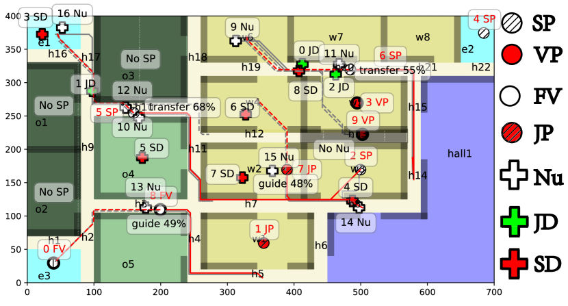
Figure 1: Snapshots of the simulated hospital environment, where a fleet of $17$ robots collaboratively guide visitors, disinfect rooms, and transport patients.

Furthermore, this drawback becomes even more apparent within dynamic scenes where contingent tasks, specified as LTL formulas are triggered by external observations and released to the whole team online. In such cases, most existing approaches compute the automaton associated with the new task, of which the synchronized product with the current automaton is derived, see [15, 16]. Thus, the size of the resulting automaton equals to the product of all automata associated with the contingent tasks, which is clearly a combinatorial blow-up. Consequently, the amount of contingent tasks that can be handled by the aforementioned approaches is limited to hand-picked examples.

To overcome this curse of dimensionality, we propose a new paradigm that is fundamentally different from the model-checking-based method. First, for an LTL formula that consists of numerous sub-formulas of smaller size, we calculate the R-posets of each sub-formula as a set of subtasks and their partial temporal constraints. Then, an efficient algorithm is proposed to compute the product of R-posets associated with each sub-formula. The resulting product of R-posets is demonstrated to be complete in the sense that it retains all subtasks from each R-poset along with their partial orderings and resolves potential conflicts. Given this product, a task assignment algorithm called the time-bound contract net (TBCN) is proposed to assign collaborative subtasks to the agents, subject to the partial ordering constraints. Last but not least, the same algorithm is applied online to dynamic scenes where contingent tasks are triggered and released by online observations. It is shown formally that the proposed method has a polynomial time and memory complexity to derive the first valid plan w.r.t. the system size and formula length. Extensive large-scale simulations and experiments are conducted for a hospital environment where service robots react to online requests such as collaborative transportation, cleaning and monitoring.

Main contribution of this work is three-fold: (i) a systematic method is proposed to tackle task formulas with length more than $30$, which overcomes the limitation of existing translation tools that can only process formulas of length less than $20$ in reasonable time; (ii) an efficient algorithm is proposed to decompose and integrate contingent tasks that are released online, which not only avoids a complete re-computation of the task automaton but also ensures a polynomial complexity to derive the first valid plan; (iii) the proposed task assignment algorithm, TBCN, is fully compatible with both static and dynamic scenarios with interactive objects.

II preliminaries

II-A Linear Temporal Logic and Büchi Automaton

The basic ingredients of Linear Temporal Logic (LTL) formulas are a set of atomic propositions $AP$ in addition to several Boolean and temporal operators. Atomic propositions are Boolean variables that can be either true or false. The syntax of LTL, as given in [1], is defined as: $\varphi\triangleq\top\;|\;p\;|\;\varphi_{1}\wedge\varphi_{2}\;|\;\neg\varphi\;|\;\bigcirc\varphi\;|\;\varphi_{1}\,\textsf{U}\,\varphi_{2},$ where $\top\triangleq\texttt{True}$, $p\in AP$, $\bigcirc$ (next), U (until) and $\bot\triangleq\neg\top$. The derivations of other operators, such as $\Box$ (always), $\Diamond$ (eventually), $\Rightarrow$ (implication) are omitted here for brevity. A complete description of the semantics and syntax of LTL can be found in [1]. Moreover, for a given LTL formula $\varphi$, there exists a Nondeterministic Büchi Automaton (NBA) as follows:

Definition 1.

A NBA $\mathcal{A}\triangleq(S,\,\Sigma,\,\delta,\,(S_{0},\,S_{F}))$ is a 4-tuple, where $S$ are the states; $\Sigma=AP$; $\delta:S\times\Sigma\rightarrow 2^{S}$ are transition relations; $S_{0},S_{F}\subseteq S$ are initial and accepting states. $\blacksquare$

An infinite word $w$ over the alphabet $2^{AP}$ is defined as an infinite sequence $W=\sigma_{1}\sigma_{2}\cdots,\sigma_{i}\in 2^{AP}$. The language of $\varphi$ is defined as the set of words that satisfy $\varphi$, namely, $\mathcal{L}(\varphi)=Words(\varphi)=\{W\,|\,W\models\varphi\}$ and $\models$ is the satisfaction relation. Additionally, the resulting run of $w$ within $\mathcal{A}$ is an infinite sequence $\rho=s_{0}s_{1}s_{2}\cdots$ such that $s_{0}\in S_{0}$, and $s_{i}\in S$, $s_{i+1}\in\delta(s_{i},\,\sigma_{i})$ hold for all index $i\geq 0$. A run is called accepting if it holds that $\inf(\rho)\cap{S}_{F}\neq\emptyset$, where $\inf(\rho)$ is the set of states that appear in $\rho$ infinitely often. A special class of LTL formula called syntactically co-safe formulas (sc-LTL) [1, 17], which can be satisfied by a set of finite sequence of words. They only contain the temporal operators $\bigcirc$, U and $\Diamond$ and are written in positive normal form where the negation operator $\neg$ is not allowed before the temporal operators.

II-B Partially Ordered Set

As proposed in our previous work [3], a relaxed partially ordered set (R-poset) over an NBA $\mathcal{B}_{\varphi}$ is a 3-tuple: $P_{\varphi}=(\Omega_{\varphi},\preceq_{\varphi},\neq_{\varphi})$, where $\Omega_{\varphi}$ is the set of subtasks and $\preceq_{\varphi},\neq_{\varphi}$ are the partial relations defined as follows.

Definition 2 (Subtasks).

[3] The set of subtasks is given by $\Omega_{\varphi}=\{(\ell,\sigma_{\ell},\sigma^{s}_{\ell}),\forall\ell=0,\dots,L\}$, where $\ell$ is the index of subtask $\omega_{\ell}$; $\sigma_{\ell}\subseteq\Sigma$ are the transition labels; $\sigma^{s}_{\ell}\subseteq\Sigma$ are the self-loop labels from Def. 1 . $\blacksquare$

Definition 3 (Partial Relations).

[3] Given two subtasks in $\omega_{h},\omega_{\ell}\in\Omega_{\varphi}$, the following two types of relations are defined: (i) “less equal”: $\preceq_{\varphi}\subseteq\Omega_{\varphi}\times\Omega_{\varphi}$. If $(\omega_{h},\omega_{\ell})\in\preceq_{\varphi}$ or equivalently $\omega_{h}\preceq_{\varphi}\omega_{\ell}$, then $\omega_{\ell}$ can only be started after $\omega_{h}$ is started; (ii) “opposed”: $\neq_{\varphi}\subseteq 2^{\Omega_{\varphi}}$. If $\{\omega_{h},\cdots,\omega_{\ell}\}\in\neq_{\varphi}$ or equivalently $\omega_{h}\neq_{\varphi}\cdots\omega_{\ell}$, subtasks in $\omega_{h},\cdots,\omega_{\ell}$ cannot all be executed simultaneously. $\blacksquare$

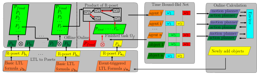
Figure 2: Framework of the proposed method. We firstly change each sub-formula into sets of R-posets with the method in Sec. IV-A . Then, we repeatedly use Alg. 1 to generate the final R-poset which satisfies all formulas of $\varPhi_{\texttt{b}}$. Thirdly, a Time-Bound Bid Net method 2 is given to determine the task sequence of each agent and object. Finally, we generate the event-triggered formula and make an online product of R-posets for online adaption if a new object is found.

III Problem Formulation

III-A Collaborative Multi-agent Systems

Consider a workspace $W\subset\mathbb{R}^{2}$ with $M$ regions of interest denoted as $\mathcal{W}\triangleq\{W_{1},\,\cdots,W_{M}\}$, where $W_{m}\in W$. Furthermore, there is a group of agents denoted by $\mathcal{N}\triangleq\{1,\cdots,N\}$ with different types $\boldsymbol{L}\triangleq\{1,\cdots,L\}$. More specifically, each agent $n\in\mathcal{N}$ belongs to only one type $l=M_{type}(n)$, where $M_{type}:\mathcal{N}\rightarrow\boldsymbol{L}$. Each type of agents $l\in\boldsymbol{L}$ is capable of providing a set of different actions denoted by $\mathcal{A}_{l}$. The set of all actions is denoted as $\mathcal{A}_{a}=\bigcup_{l\in L}\mathcal{A}_{l}=\{a_{1},\cdots,a_{n_{\mathcal{C}}}\}$. Without loss of generality, the agents can navigate between each region via the same transition graph, i.e., $\mathcal{G}=(\mathcal{W},\,\rightarrow_{\mathcal{G}},\,d_{\mathcal{G}})$, where $\rightarrow\subseteq\mathcal{W}\times\mathcal{W}$ represents the allowed transitions; and $d_{\mathcal{G}}:\rightarrow_{\mathcal{G}}\rightarrow\mathbb{R}_{+}$ maps each transition to its duration.

Moreover, there is a set of interactive objects $\mathcal{O}\triangleq\{o_{1},\cdots,o_{U}\}$ with several types $\mathcal{T}\triangleq\{T_{1},\cdots,T_{H}\}$ scattered across the workspace $W$. These objects are interactive and can be transported by the agents from one region to another. An interactive object $o_{u}\in\mathcal{O}$ is described by a three-tuple:

$$o_{u}\triangleq(T_{h_{u}},\,t_{u},\,W^{p}_{u}),$$ (1)

where $T_{h_{u}}\in\mathcal{T}$ is the type of object; $t_{u}\in R^{+}$ is the time when $o_{u}$ appears in workspace $W$; $W^{p}_{u}:R^{+}\rightarrow\mathcal{W}$ is a function that $W^{p}_{u}(t)$ returns the region of $o_{u}$ at time $t\geq t_{u}$; and $W^{p}_{u}(t_{u})\subseteq W$ is the initial region. Additionally, new objects appear in $W$ over time and are then added to the set $\mathcal{O}$. With a slightly abusive of notation, we denote the set of initial objects $\mathcal{O}_{in}$ that already exist in $W$ and the set of online objects $\mathcal{O}_{on}$ that are added during execution, i.e., $\mathcal{O}=\mathcal{O}_{in}\cup\mathcal{O}_{on}$.

To interact with the objects, the agents can provide a series of collaborative behaviors $\mathcal{C}\triangleq\{C_{1},\dots,C_{K}\}$. A collaborative behavior $C_{k}\in\mathcal{C}$ is a tuple defined as follows:

$$C_{k}\triangleq(o_{u_{k}},\{(a_{i},n_{i}),\,i\in\boldsymbol{L}_{k}\})$$ (2)

where $o_{u_{k}}\in\mathcal{O}\cup\{\emptyset\}$ is the interactive object if any; $a_{i}\in\mathcal{A}_{a}$ is the set of cooperative actions required; $0<n_{i}\leq N$ is the number of agents to provide the action $a_{i}$; and $\boldsymbol{L}_{k}$ is the set of action indices associated with the behavior $C_{k}$. Also, $d_{k}$ denotes the execution time of $C_{k}$.

Remark 1.

A behavior can only be executed if the required object is at the desired region. Since objects can only be transported by the agents, it is essential for the planning process to find the correct order of these transporation behaviors. Related works [2, 14] build a transition system to model the interaction between objects and agents, the size of which grows exponentially with the number of agents and objects. $\blacksquare$

Remark 2.

The behavior $\mathcal{C}$ above is similar to the atomic unit of capability temporal logic (CaTL) in [9, 18], which only models static scenarios without interactive objects. $\blacksquare$

III-B Task Specifications

Consider the following two types of atomic propositions: (i) $p^{l}_{m}$ is true when any agent of type $l\in\boldsymbol{L}$ is in region ${W}_{m}\in{\mathcal{W}}$; $p^{r}_{m}$ is true when any object of type $r\in\mathcal{T}$ is in region ${W}_{m}\in{\mathcal{W}}$; Let $\mathbf{p}\triangleq\{p^{l}_{m},\,\forall{W}_{m}\in{\mathcal{W}},l\in L\}\bigcup\{p^{r}_{m},\,\forall{W}_{m}\in{\mathcal{W}},r\in\mathcal{R}\}$. (ii) $(C_{k})^{{u_{k}}}_{k_{1},k_{2}}$ is true when the collaborative behavior $C_{k}$ in (2) is executed with object $o_{u_{k}}$, starting from region ${W}_{k_{1}}$ and ending in region ${W}_{k_{2}}$. Let $\mathbf{c}\triangleq\{(C_{k})^{u_{k}}_{k_{1},k_{2}},\forall C_{k}\in\mathcal{C},o_{u_{k}}\in\mathcal{O},\forall{W}_{k_{1}},{W}_{k_{2}}\in{\mathcal{W}}\}$. Given these propositions, the team-wise task specification is specified as a sc-LTL formula over $\{\mathbf{p},\mathbf{c}\}$:

$$\varphi=(\bigwedge_{i\in\mathcal{I}}\varphi_{\texttt{b}_{i}})\wedge(\bigwedge_{o_{u}\in\mathcal{O}_{on}}\varphi_{\texttt{e}_{u}}),$$ (3)

where $\{\varphi_{\texttt{b}_{i}},\,i=1,\cdots,I\},\{\varphi_{\texttt{e}_{u}},\,o_{u}\in\mathcal{O}_{on}\}$ are two sets of sc-LTL formulas over $\{\mathbf{p},\mathbf{c}\}$. The $\varphi_{\texttt{b}_{i}}$ is specified in advance while $\varphi_{\texttt{e}_{u}}$ is generated online when a new object $o_{u}$ is added to $\mathcal{O}_{on}$. The detailed syntax of sc-LTL is introduced in Sec. II-A.

To satisfy the LTL formula $\varphi$, the complete action sequence of all agents is defined as:

$$\mathcal{J}=(J_{1},J_{2},\cdots,J_{N}),$$ (4)

where $J_{n}\in\mathcal{J}$ is the sequence of $(t_{k},\mathcal{C}_{k},a_{k})$, which means that agent $n$ executes behavior $\mathcal{C}_{k}$ by providing the collaborative service $a_{k}\in\mathcal{A}_{a}$ at time $t_{k}$. In turn, the sequences of actions for an interactive object is defined as:

$$\mathcal{J}^{o}=(J^{o}_{1},J^{o}_{2},\cdots,J^{o}_{U}),$$ (5)

where $J^{o}_{u}=(t_{k},\mathcal{C}_{k})\cdots$ is the sequence of tasks associated with object $o_{u}\in\mathcal{O}$. The task pair $(t_{k},\mathcal{C}_{k})$ is added to $J^{o}_{u}$ if object $o_{u}$ joins behavior $\mathcal{C}_{k}$ at time $t_{k}$. Assume that the duration of formula $\varphi_{\texttt{b}_{i}},\varphi_{\texttt{e}_{i}}$ from being published to being satisfied is given by $D_{i}$, the average efficiency is defined by $\eta\triangleq\frac{\sum_{C_{k}\in J}|\boldsymbol{L}_{k}|d_{k}}{D_{i}}$ as the average duration of all subtasks.

III-C Problem Statement

Problem 1.

Given the sc-LTL formula $\varphi$ defined in (3), synthesize and update the motion and action sequence of agents $\mathcal{J}$ and objects $\mathcal{J}_{o}$ for each agent $n\in\mathcal{N}$ to satisfy $\varphi$ and maximize execution efficient $\eta$. $\blacksquare$

Although maximizing the task efficiency of a multi-agent system is a classical problem, the combination of interactive objects, long formulas and contingent tasks imposes new challenges in terms of exponential complexity [6, 14] and online adaptation [15].

IV Proposed Solution

As shown in Fig. 2, the proposed solution consists of four main components: i) LTL to R-posets, where the R-posets associated with each known formula in $\varphi_{\texttt{b}_{i}}\in\Phi_{\texttt{b}}$ is generated in parallel; ii) Product of R-posets, where the product of existing R-posets is computed incrementally; iii) Task assignment, where subtasks are assigned to the agents given the temporal and spatial constraints specified in the R-posets; iv) Online adaptation, where the product of R-posets is updated given the contingent tasks, and the assignment is adjusted accordingly.

IV-A LTL to R-posets

To avoid the exponential complexity when translating the formula $\varphi$ into NBA, the sub-formulas $\varphi_{\texttt{b}_{i}}\in\varPhi_{\texttt{b}}$ are converted first to R-posets by the method $\texttt{compute\_poset}(\cdot)$ proposed in our earlier work [3]. Particularly, each sub-formula $\varphi_{\texttt{b}_{i}}\in\varPhi_{\texttt{b}}$ is converted into a set of R-posets, denoted by $\mathcal{P}_{\texttt{b}_{i}}=\{P^{\texttt{b}_{i}}_{j}\}$, where $P^{\texttt{b}_{i}}_{j}=(\Omega_{j},\preceq_{j},\neq_{j})$ follows the notations from Def. 3; $\Omega_{j}=(\ell,\sigma_{\ell},\sigma_{\ell}^{s})$ is the set of subtasks each of which consists of the index $\ell$, the subtask labels $\sigma_{\ell}$ and the self-loop labels $\sigma^{s}_{\ell}$ as defined in Def. 2. It is proven that a word is accepting if it satisfies all the constraints imposed by $\mathcal{P}_{\texttt{b}_{i}}$.

Definition 4 (Language of R-poset).

[3] Given a word $w=\sigma^{\prime}_{1}\sigma^{\prime}_{2}\cdots$ satisfying R-poset $P=(\Omega,\preceq,\neq)$, denoted as $w\models P$, it holds that: i) given $\omega_{i_{1}}=(i_{1},\sigma_{i_{1}},\sigma^{s}_{i_{1}})\in\Omega$, there exist $j_{1}$ with $\sigma_{i_{1}}\subseteq\sigma^{\prime}_{j_{1}}$ and $\sigma^{s}_{j_{1}}\cap\sigma^{\prime}_{m_{1}}=\emptyset,\forall m_{1}<j_{1}$; ii) $\forall(\omega_{i_{1}},\omega_{i_{2}})\in\preceq,\exists j_{1}\leq j_{2},\sigma_{i_{2}}\subseteq\sigma^{\prime}_{j_{2}},\forall m_{2}<{j_{2}},\sigma^{s}_{j_{2}}\subseteq\sigma^{\prime}_{m_{2}}$; iii) $\forall(\omega_{i_{1}},\cdots,\omega_{i_{n}})\in\neq,\exists\ell\leq n,\sigma_{i_{\ell}}\not\subseteq\sigma^{\prime}_{j_{1}}$. Language of R-poset $P$ is the set of all word $w$ that satisfies $P$, denoted by $\mathcal{L}(P)\triangleq\{w|w\vDash P\}$. $\blacksquare$

Assuming that $\mathcal{P}_{b_{i}}=\{P^{b_{i}}_{1},P^{b_{i}}_{2},\cdots\}$ is the set of all possible R-posets, it is shown in Lemma 3 of our previous work [3] that: (i) $\mathcal{L}(P^{b_{i}}_{j})\subseteq\mathcal{L}(\mathcal{B}_{b_{i}}),P^{b_{i}}_{j}\in\mathcal{P}^{b_{i}}_{\varphi}$; (ii) $\bigcup_{P^{b_{i}}_{j}\in\mathcal{P}^{b_{i}}_{\varphi}}\mathcal{L}(P_{i})=\mathcal{L}(\mathcal{B}_{b_{i}})$. In other words, the R-posets contain the necessary information for subsequent steps.

IV-B Product of R-posets

To generate a complete R-poset for the whole task $\varPhi_{\texttt{b}}$, we define the product of R-posets as follows:

Definition 5 (Product of R-posets).

The product of two posets $P_{1},P_{2}$ is defined as a set of R-posets $\mathcal{P}^{r}\triangleq\{P^{\prime}_{1},P^{\prime}_{2},\cdots\}$, denoted as $\mathcal{P}^{r}=P_{1}\bigotimes P_{2}$ where $P^{\prime}_{i}$ satisfies two conditions: (i) $w\in\mathcal{L}(P_{1})\cap\mathcal{L}(P_{2}),\forall w\in\mathcal{L}(P^{\prime}_{i}),\forall P^{\prime}_{i}\in\mathcal{P}^{r}$; (ii) $w\in\bigcup_{P^{\prime}_{i}\in\mathcal{P}^{r}}\mathcal{L}(P^{\prime}),\forall w\in\mathcal{L}(P_{1})\cap\mathcal{L}(P_{2})$. $\blacksquare$

Thus, to get the R-poset of formula $\varphi_{1}\land\varphi_{2}$, there is no need to generate the NBA of $\varphi_{1}\land\varphi_{2}$. Instead, we only generate the NBA of $\varphi_{1}$ and $\varphi_{2}$ to find the R-poset $P_{1}$ of $\varphi_{1}$ and $P_{2}$ of $\varphi_{2}$. Then, we generate a set of R-posets $\mathcal{P}^{r}$ by $P_{1},P_{2}$, which satisfies the two conditions in Def.5. Here we present an anytime algorithm $\texttt{Poset\_Prod}(\cdot)$ as in Alg. 1. It generates the product of two R-posets $P_{1}=(\Omega_{1},\preceq_{1},\neq_{1}),P_{2}=(\Omega_{2},\preceq_{2},\neq_{2})$ in the following two steps.

Input : R-poset $P_{1}$, R-poset $P_{2}$, Time budget $t_{b}$

Output : Product R-poset set $\mathcal{P}_{final}$.

1 $\mathcal{P}_{final}=\{\}$,$que=[(\Omega=\Omega_{1},M_{\Omega})]$

2 while  $|que|>0$ and $t<t_{b}$  do

3       $\Omega^{\prime},M^{\prime}_{\Omega}=que.pop()$

4       for $\omega^{2}_{i}\in\Omega_{2}/R(M^{\prime}_{\Omega})$ do

5             for  $\omega^{1}_{j}\in\Omega_{1}/D(M^{\prime}_{\Omega})$, $\omega^{2}_{i}\models\omega^{1}_{j}$ or $\omega^{1}_{j}\models\omega^{2}_{i}$ do

6                   Create $\hat{\Omega}^{\prime},\hat{M}^{\prime}_{\Omega}$ by (6), add them to $que$

7            

8            Create $\hat{\Omega}^{\prime},\hat{M}^{\prime}_{\Omega}$ by (7), add them to $que$

9      for $(\Omega,M_{\Omega})\in que$ with $|D(M_{\Omega})|=|\Omega_{2}|$ do

10             Remove $(\Omega,M_{\Omega})$, $\preceq=\preceq_{\varphi_{1}}\cup M_{\Omega}(\preceq_{\varphi_{2}})$

11             Update $\Omega$ by (9),(10)

12             Find potential ordering. Update $\preceq$, $\Omega$

13            

14            if no conflicts between $\Omega,\preceq$ then

15                   calculate $\neq$, add $\{\Omega,\preceq,\neq\}$ into $\mathcal{P}_{final}$

16            update $t$, if $t<t_{b}$ then return $\mathcal{P}_{final}$

17      

return $\mathcal{P}_{final}$

Algorithm 1 $\texttt{Poset\_Prod}(\cdot)$: Calculate the product between two R-posets

(i) Composition of substasks. In this step, we generate all possible combinations of subtasks which can satisfy both $\Omega_{1}$ and $\Omega_{2}$ in Line 1-1. Namely, a set of subtasks $\Omega^{\prime}=\{\omega^{\prime}_{1},\cdots,\omega^{\prime}_{n^{\prime}}\}$ satisfies $\Omega_{1}$ if for each $\omega^{1}_{i}=(i,{\sigma^{1}_{i}},{\sigma^{s1}_{i}})\in\Omega_{1}$, there is a subtask $\omega^{\prime}_{j}=(j,{\sigma_{j}}^{\prime},{\sigma^{s}_{j}}^{\prime})\in\Omega^{\prime}$ satisfying $\sigma^{1}_{i}\subseteq\sigma^{\prime}_{j}$ and $\sigma^{s1}_{i}\subseteq{\sigma^{s}_{j}}^{\prime}$, or $\omega^{\prime}_{j}\models\omega^{1}_{i}$ for brevity. Since $\Omega^{\prime}=\Omega_{1}$ in Line 1, $\Omega^{\prime}$ clearly satisfies $\Omega_{1}$ with $\forall\omega^{1}_{i}\in\Omega_{1},\omega^{\prime}_{i}\models\omega^{1}_{i}$. Then, a mapping $M_{\Omega}:\Omega_{2}\rightarrow\Omega^{\prime}$ is defined to store the satisfying relationship from $\Omega_{2}$ to $\Omega^{\prime}$, and $\mathcal{D}(M_{\Omega})\in\Omega_{2}$ is the domain of $M_{\Omega}$, $\mathcal{R}(M_{\Omega})$ is the range of $M_{\Omega}$. As all relations are unknown, $M_{\Omega}$, $\mathcal{D}(M_{\Omega})$ and $\mathcal{R}(M_{\Omega})$ are initially set to empty. Namely, if $\omega^{\prime}_{j}\models\omega^{2}_{i}$, we will store $M_{\Omega}(\omega^{2}_{i})=\omega^{\prime}_{j}$ and $M^{-1}_{\Omega}(\omega^{\prime}_{j})=\omega^{2}_{i}$, and add $\omega^{2}_{i}$ into $\mathcal{D}(M_{\Omega})$, $\omega^{\prime}_{j}$ into $R(M_{\Omega})$, where $M^{-1}_{\Omega}$ is the inverse function of $M_{\Omega}$. Then, in Lines 1-1, we use a depth-first-search (DFS) to construct all possible sets of subtasks $\hat{\Omega}^{\prime}$ and corresponding $\hat{M}^{\prime}_{\Omega}$. In Line 1 -1, we check all possible combinations of unrecorded subtask $(\omega^{1}_{j},\omega^{2}_{i}),\omega^{1}_{j}\in\Omega_{1}/R(M^{\prime}_{\Omega}),\omega^{2}_{i}\in\Omega_{2}/D(M^{\prime}_{\Omega})$ whether $\omega^{1}_{j}\models\omega^{2}_{i}$ or $\omega^{2}_{i}\models\omega^{1}_{j}$ holds. If so, we can create a new set of subtasks $\hat{\Omega}^{\prime}$ and a new mapping function $\hat{M}^{\prime}_{\Omega}$ based on $\Omega^{\prime},M^{\prime}_{\Omega}$ in Line 1 as follows:

$$\hat{\Omega}^{\prime} =\Omega^{\prime},\,\hat{\omega}^{\prime}_{j}=(j,\sigma^{1}_{j}\cup\sigma^{2}_{i},\,\sigma^{s1}_{j}\cup\sigma^{s2}_{i}),$$ (6)

$$\hat{M}^{\prime}_{\Omega} =M^{\prime}_{\Omega},\,\hat{M}^{\prime}_{\Omega}(\omega^{2}_{i})=\omega^{\prime}_{j},$$

which means the subtask $\omega^{\prime}_{j}$ in $\Omega^{\prime}$ can be executed to satisfy $\omega^{1}_{j},\omega^{2}_{i}$. Moreover, for each subtasks $\omega^{2}_{i}\in\Omega_{2}/R(M^{\prime}_{\Omega})$, we can always create a set of subtasks $\hat{\Omega}^{\prime}$ and the corresponding mapping function $\hat{M}^{\prime}_{\Omega}$ in Line 1 by appending $\omega^{2}_{i}$ into $\hat{\Omega}^{\prime}$ as $\hat{\omega}^{\prime}_{j}$ such that $\hat{\omega}^{\prime}_{j}\models\omega^{2}_{i}$ holds, i.e.,

$$\hat{\Omega}^{\prime}=\Omega^{\prime},j=|\Omega^{\prime}|+1,\hat{\omega}^{\prime}_{j}=\omega^{2}_{i};$$ (7)

$$\hat{M}^{\prime}_{\Omega}=M^{\prime}_{\Omega},\hat{M}^{\prime}_{\Omega}(\omega^{2}_{i})=\omega^{\prime}_{j},$$

which means the subtask $\omega^{\prime}_{j}$ can be executed to satisfy $\omega^{2}_{i}$.

This step ends if the time budget $t_{b}$ or the search sequence $que$ exhausted as in Line 1. Once $|D(M_{\Omega})|=|\Omega_{2}|$ as in Line 1, it means the $\Omega^{\prime}$ satisfying $\Omega_{1},\Omega_{2}$ is already found. In this case, the next step is triggered.

(ii) Relation calculation. In Lines 1 - 1, given the set of subtasks $\Omega$ and the mapping function $M_{\Omega}$, we calculate the partial relations among them and build a product R-poset $P$. Firstly, in Line 1, we construct the “less-equal” constraint $\preceq$ as follows:

$$\preceq=\preceq_{1}\cup\{(M_{\Omega}({\omega^{2}_{\ell_{1}}}),M_{\Omega}(\omega^{2}_{\ell_{2}}))|(\omega^{2}_{\ell_{1}},\omega^{2}_{\ell_{2}})\in\preceq_{2}\},$$ (8)

which inherits the both less equal relations $\preceq_{1}$ in $P_{1}$ and $\preceq_{2}$ in $P_{2}$. Then, we update $\Omega$ in Line 1 to consider the constraints imposed by the self-loop labels in other subtasks. Specifically, if a new relation $(\omega_{i},\omega_{j})$ is added to $\preceq$ by $(M^{-1}_{\Omega}(\omega^{2}_{i}),M^{-1}_{\Omega}(\omega^{2}_{j}))\in\preceq_{2}$ while $(\omega^{1}_{i},\omega^{1}_{j})\not\in\preceq_{1}$ holds, $\omega_{i}$ is required to be executed before $\omega_{j}$ although $(\omega^{1}_{i},\omega^{1}_{j})$ does not belong to $\preceq_{1}$ of $P_{1}$. In this case, $\sigma_{i}$ and $\sigma^{s}_{i}$ are updated to guarantee the satisfaction of the self-loop labels $\sigma^{s}_{j}$ before executing $\sigma_{j}$. For each subtask $\omega_{i}$, the sets of newly-added suf-subtasks from $\preceq_{1},\preceq_{2}$ are defined as $S^{1}_{p},S^{2}_{p}$, i.e.,

$$S^{1}_{p}= \{\omega_{j}|(\omega_{i},\omega_{j})\in\preceq,(\omega^{1}_{i},\omega^{1}_{j})\not\in\preceq_{1}\},$$ (9)

$$S^{2}_{p}= \{M^{-1}_{\Omega}(\omega_{j})|(\omega_{i},\omega_{j})\in\preceq,(M^{-1}_{\Omega}(\omega^{2}_{i}),M^{-1}_{\Omega}(\omega^{2}_{j}))\not\in\preceq_{2}\},$$

in which are the subtasks that should be executed after $\omega_{i}$ although $\preceq_{1}$ or $\preceq_{2}$ does not require. Thus, the action labels $\sigma_{i}$ and self-loop labels $\sigma^{s}_{i}$ in $\omega_{i}=(i,\sigma_{i},\sigma^{s}_{i})$ are updated accordingly as follows:

$$\hat{\sigma}=\bigcup_{\omega^{1}_{\ell}\in S^{1}_{p}}\sigma^{s1}_{\ell}\cup\bigcup_{\omega^{2}_{\ell}\in S^{2}_{p}}\sigma^{s2}_{\ell},\sigma^{s}_{i}=\hat{\sigma}\cup\sigma^{s}_{i},\sigma_{i}=\hat{\sigma}\cup\sigma_{i},$$ (10)

in which $\sigma^{s}_{i}$ and $\sigma_{i}$ should be executed under the additional labels $\hat{\sigma}$ thus the self-loop labels of $S^{1}_{p},S^{2}_{p}$ are satisfied. In Line 1, we find the potential ordering by checking whether a subtask $\sigma^{s}_{i}$ is in conflicts with another subtask $\sigma_{j}$ while $(\omega_{i},\omega_{j})\not\in\preceq$. If so, an additional ordering $(\omega_{i},\omega_{j})$ will be added to $\preceq$ and $\Omega$ is updated following (9) and (10). Regarding the set of subtasks $\Omega$ that have no conflicts in $\preceq$, we can generate its “not-equal” relations $\neq$ by a simple combination as $\neq_{1}\cup\Big{\{}\{{M_{\Omega}(\omega_{\ell_{i}})}\}|\{\omega_{\ell_{i}}\}\in\neq_{2}\Big{\}}$. Lastly, the resulting poset $P_{i}=(\Omega,\preceq,\neq)$ is added to $\mathcal{P}_{final}$.

As shown in Fig. 2, the above procedure is applied recursively for each pair of R-posets to compute the complete set of R-posets for formula $\varPhi_{b}$. Namely, the first product is computed as $\mathcal{P}_{final}=P_{\texttt{b}_{1}}\otimes P_{\texttt{b}_{2}}$ in the first round. Then, we fetch the best R-poset $P_{final}$ in $\mathcal{P}_{final}$ according to the efficiency measure proposed in our earlier work. It is multiplied with the next $P_{b_{i}}$ as $\mathcal{P}_{final}=P_{final}\otimes P_{\texttt{b}_{i}}$. This procedure is repeated until time budget exhausted or all possible R-posets are found. Thus, the anytime property of calculating the R-posets of $\varphi$ is ensured, so that we can quickly get a $P_{final}$ satisfies all $P_{\texttt{b}_{i}}$ and then continue to get more R-posets.

IV-C Task Assignment

The LTL formulas are converted into a R-poset $P_{c}=(\Omega_{c},\preceq_{c},\neq_{c})$, where each subtask $\omega_{i}\in\Omega_{c}$ represents a collaborative behavior $C_{j}$. Thus, we can redefine the action sequence of each agent $J_{n}\in\mathcal{J}$ as $J_{n}=[(t_{k},\omega_{k},a_{k}),\cdots]$ and the action sequence of each object $J^{o}_{u}\in\mathcal{J}_{o}$ as $J^{o}_{u}=[(t_{k},\omega_{k},a_{k}),\cdots]$. in which we replace the cooperative behavior $C_{k}$ with $\omega_{k}$ since $C_{k}\in\sigma_{k}$.

Input :  R-poset $P_{c}=(\Omega_{c},\preceq_{c},\neq_{c})$

Output : Updated plans $\mathcal{J}$, $\mathcal{J}_{o}$

1 $\Omega_{u}=\Omega_{c},\Omega_{as}=\{\},\mathcal{J}=[],\mathcal{J}_{o}=[]$.

2 while $|\Omega_{u}|>0$ do

3       Get feasible subtask $\Omega_{fe}$ based on $\Omega_{as}$,$P_{c}$ by (11)

4       for $\omega_{i}\in\Omega_{fe}$ do

5             Get time bounds and generate $\mathcal{J}^{i},\mathcal{J}^{i}_{o}$

6      

7      Choose $\omega_{i}$, update $\Omega_{u}$, $\Omega_{as}$, $\mathcal{J}=\mathcal{J}^{i},\mathcal{J}_{o}=\mathcal{J}^{i}_{o}$

8      

9

return $\mathcal{J},\mathcal{J}_{o}$

Algorithm 2 $\texttt{TW\_ContractNet}(\cdot)$: Online task assignment by time bound contract net.

As summarized in Alg. 2, we propose a sub-optimal algorithm called Time Bound Contract Net (TBCN) for the task assignment. Compared with the classical Contract Net method [19], the main differences are: (i) the assigned subtasks should satisfy the temporal constraints in $\preceq_{c},\neq_{c}$; (ii) the cooperative task should be fulfilled by multiple agents; and (iii) interactive objects should be considered as an additional constraints. To begin with, we initialize the set of unassigned subtasks as $\Omega_{u}=\Omega_{c}$, the set of assigned subtasks $\Omega_{as}=\{\}$, and the task sequence of agents $\mathcal{J}$ and objects $\mathcal{J}_{o}$ as Line 2. For the ordering constraints $\preceq_{c}$, if $(\omega_{j},\omega_{i})\in\preceq_{c}$, assigning $(t_{k_{j}},\omega_{j},a_{k_{j}})$ to a task sequence $J_{i}=\cdots(t_{k_{i}},\omega_{i},a_{k_{i}})$ will violate such constraints. Thus, we add a mechanism to avoid creating such cases, i.e., only assign the set of feasible subtasks $\Omega_{fe}$ based on $\Omega_{as}$ in Line 2 :

$$\Omega_{fe}=\{\omega_{i}|\omega_{i}\in\Omega_{u},\forall(\omega_{j},\omega_{i})\in\preceq_{c},\omega_{j}\in\Omega_{as}\},$$ (11)

in which the subtasks may lead to unfeasible action sequences being eliminated.

Then, in Line 2 , any constraint of a subtask $\omega_{i}\in\Omega_{fe}$ is considered as a time instance $t_{1}\in\mathbb{R}^{+}$ which means such constraint can be satisfied after $t_{1}$. Without loss of generality, we assume $\sigma_{i}=\{(C_{k})^{u_{k}}_{k_{1},k_{2}}\}$ meaning that the agents need to execute the behavior $C_{k}$ from region $W_{k_{1}}$ to region $W_{k_{2}}$ using object $u_{k}$. Here, we use three kinds of time bounds to manage the biding process: the global time bound $t^{\omega}_{i}$, the object time bound $t^{o}_{u_{k}}$ and the set of local time bounds $\boldsymbol{T_{s}}$. The global time bound $t^{\omega}_{i}$ is the time instance that the ordering constraints $\preceq_{c}$ and conflict constraints $\neq_{c}$ will be satisfied if behavior $(C_{k})^{u_{k}}_{k_{1},k_{2}}$ is executed after $t^{\omega}_{i}$. For the required object $u_{k}$, assuming its participated last task is $\mathcal{J}^{o}_{u_{k}}[-1]=(t_{\ell},\omega_{\ell})$, the object time bound $t^{o}_{u_{k}}$ should satisfy that:

$$W^{p}_{u}(t)=W_{k_{1}},t\geq t_{\ell}+d_{\ell},,\forall t\geq t^{o}_{u_{k}},$$ (12)

which means the object $u_{k}$ will be at the starting region $W_{k_{1}}$ of the current behavior $(C_{k})^{u_{k}}_{k_{1},k_{2}}$ and ready for it after $t^{o}_{u_{k}}$. Additionally, we set $t^{o}_{u_{k}}=\infty$ if the object is not at $W_{k_{1}}$ after the action sequence $\mathcal{J}^{o}_{u_{k}}$, and we set $t^{o}_{u_{k}}=0$ if the behavior $(C_{k})^{u_{k}}_{k_{1},k_{2}}$ does not require object as $u_{k}=\emptyset$. The set of local time bound is defined as $\boldsymbol{T_{s}}=\{(\mathcal{A}_{n},t^{a}_{n})_{n\in\mathcal{N}}\}$, where $\mathcal{A}_{n}$ is the set of actions agent $n$ can provide for behavior $(C_{k})^{u_{k}}_{k_{1},k_{2}}$, and $t^{a}_{n}$ is the earliest time agent $n$ can arrive region $W_{k_{1}}$. $(\mathcal{A}_{n},t^{a}_{n})$ means agent $n$ can begin behavior $(C_{k})^{u_{k}}_{k_{1},k_{2}}$ after time $t^{a}_{n}$ by providing one of action $a_{\ell}\in\mathcal{A}_{n}$. Using these time bounds, we can determine the agents and their providing actions and generate a new party assignment $\mathcal{J}^{i},\mathcal{J}^{i}_{o}$ to minimize the ending time of subtask $\omega_{i}$. The efficiency $\eta$ of each assignment $\mathcal{J}^{i},\mathcal{J}^{i}_{o},\omega_{i}\in\Omega_{u}$ is calculated in Line 2, and the subtask with max efficiency will be chosen. Afterwards, the chosen subtask is removed from $\Omega_{un}$ and added to $\Omega_{as}$. The action sequences $\mathcal{J},\mathcal{J}_{o}$ are updated accordingly as $\mathcal{J}=\mathcal{J}^{i},\mathcal{J}_{o}=\mathcal{J}^{i}_{o}$ for the next iteration.

Remark 3.

As this algorithm can only assign the subtask in $\Omega$ of R-poset $P_{final}=(\Omega,\preceq,\neq)$, the R-poset should follow an assumption: There exists an action sequence order under the ordering constraints $\preceq$ and conflicts constraints $\neq$ that can transform and interact with the objects in order. That means the formula should not require a behavior to transfer an object at region $W_{1}$ before it has been moved there beforehand.

IV-D Online Adaption

As there are objects added to the workspace online, the agents are required to update their action sequences to satisfy the contingent formulas. The online adaptation has two important parts: the adaptation of R-posets and the adaptation of task sequences. The adaptation of R-posets is to update the R-poset $P_{final}$ based on $P_{final}$ and the R-poset $P_{e_{u}}$ of contingent formula $\varphi_{\texttt{e}_{u}}$, instead of recomputing the R-poset associated with the whole formula from scratch. The definition of online product between on existing R-poset $P_{1}$ and contingent $P_{2}$ is given as:

Definition 6 (Online Product of R-posets).

Given a finite word $w_{0}$, the online product of two R-posets $P_{1},P_{2}$ is defined as a set of R-posets $\mathcal{P}^{r}=\{P^{\prime}_{1},P^{\prime}_{2},\cdots\}$, denoted as $\mathcal{P}^{r}=P_{1}\widetilde{\bigotimes}P_{2}$ where $P^{\prime}_{i}$ satisfies two conditions: (i) if $w_{0}w\in\mathcal{L}(P_{1}),w\in\mathcal{L}(P_{2})$, then $w_{0}w\in\bigcup_{P^{\prime}_{i}\in\mathcal{P}^{r}}\mathcal{L}(P^{\prime})$; (ii) if $w_{0}w\in\mathcal{L}(P^{\prime}_{i})$, $P^{\prime}_{i}\in\mathcal{P}^{r}$, then $w_{o}w\in\mathcal{L}(P_{1}),w\in\mathcal{L}(P_{2})$. $\blacksquare$

The difference between $\otimes$ and $\widetilde{\otimes}$ is that the finished word $w_{0}$ only effects the R-poset $P_{1}$ but not the R-poset $P_{2}$ in $\widetilde{\otimes}$. Thus, once a new formula $\varphi_{\texttt{e}_{u}}$ is added, we will collect the set of finished behaviers $\Omega_{f}\subseteq\Omega_{1}$ from current word $w_{0}$, which cannot effect the R-poset $P_{\texttt{e}_{u}}$ of $\varphi_{\texttt{e}_{u}}$. The method to compute the online product is similar to the Alg. 1, with two minor modifications. Namely, the set of finished subtasks $\Omega_{f}$ is added as an additional input and the condition of the for loop in Line 1 is changed to: for $\omega^{1}_{j}\in\Omega_{1}/D(M^{\prime})/\Omega_{f}$, with $\omega^{2}_{i}\models\omega^{1}_{j}$ or $\omega^{1}_{j}\models\omega^{2}_{i}$ holds. Since $\omega^{1}_{i}$ is already accomplished before $P_{2}$ is proposed, there is no need to require another subtask to satisfy $\omega^{1}_{i}$ again.

In the adaption of task sequences, the task sequences of agents and objects $\mathcal{J},\mathcal{J}_{o}$ are updated given the updated final R-poset $P_{final}=(\Omega,\preceq,\neq)$. First, we compute a set of essential conflict subtasks $\Omega_{ec}$, defined as:

$$\Omega_{ec}= \{\omega_{i}|\omega_{i}\preceq\omega_{j},t_{i}\geq t_{j},\forall\omega_{i},\omega_{j}\in\Omega_{1}/\Omega_{f}\}\cup$$ (13)

$$\{\omega_{i}|\omega_{i}\neq\omega_{j},t_{j}\leq t_{i}\leq t_{j}+d_{j},\forall\omega_{i},\omega_{j}\in\Omega_{1}/\Omega_{f}\},$$

in which is the subtask conflicts the updated ordering constraints $\preceq$ and conflict constraints $\neq$. Then, we compute the set of subtasks $\Omega_{conf}$ that should be removed from $\mathcal{J},\mathcal{J}_{o}$:

$$\Omega_{conf}= \{\omega_{j}|\omega_{i}\preceq\omega_{j},\forall\omega_{i}\in\Omega_{1}/\Omega_{f},\forall\omega_{j}\in\Omega_{ec}\}\cup\Omega_{ec},$$ (14)

in which are the subtasks in $\Omega_{ec}$ and the subtasks whose pre-subtasks will be removed. Given $\Omega_{conf}$ above, we can use $\texttt{TW\_ContractNet}(\cdot)$ to generate a new task sequence for each robot and object. After removing all the subtasks in $\Omega_{conf}$ from $\mathcal{J},\mathcal{J}_{o}$. It is worth mentioning that the step of initialization in Line 2 is changed to: $\Omega_{as}=\Omega_{1}/\Omega_{conf},\Omega_{u}=\Omega_{c}/\Omega_{as}$ and $\mathcal{J},\mathcal{J}_{o}$ are the previous solution with $\Omega_{conf}$ been removed.

IV-E Correctness, Completeness and Complexity Analysis

Theorem 1 (Correctness).

Given two R-posets $P_{\varphi_{1}}=(\Omega_{\varphi_{1}},\preceq_{\varphi_{1}},\neq_{\varphi_{1}}),P_{\varphi_{2}}=(\Omega_{\varphi_{2}},\preceq_{\varphi_{2}},\neq_{\varphi_{2}})$ generated from $\mathcal{B}_{\varphi_{1}},\mathcal{B}_{\varphi_{2}}$, we have $\mathcal{L}(P_{j})\subseteq\mathcal{L}(P_{\varphi_{1}})\cap\mathcal{L}(P_{\varphi_{2}})$, where $P_{j}\in\mathcal{P}_{final}$, $\mathcal{P}_{final}$ is calculated by Alg.1 . $\blacksquare$

Proof.

If a word $w=\sigma^{\prime}_{1}\sigma^{\prime}_{2}\cdots$ satisfies $P_{j}=(\Omega_{j},\preceq_{j},\neq_{j}),P_{j}\in\mathcal{P}_{final}$, it satisfies the three conditions mentioned in Def. 4. In first condition, due to Line 1-1 of Alg. 1, we can infer that for any $\omega^{1}_{n}=(n,\sigma^{1}_{n},\sigma^{s1}_{n})\in\Omega_{\varphi_{1}},$ there exists $\omega_{n}=(n,\sigma_{n},\sigma^{s}_{n})\in\Omega_{j}$, with $\sigma^{1}_{n}\subseteq\sigma_{n},\sigma^{s1}_{n}\subseteq\sigma^{s}_{n}$. Thus, we have $\sigma^{1}_{i_{1}}\subseteq\sigma_{i_{1}}\subseteq\sigma^{\prime}_{\ell_{1}}$ and $\sigma^{s1}_{i_{1}}\cap\sigma^{\prime}_{m_{1}}=\emptyset,\forall m_{1}<\ell_{1}$, which indicates that $w$ satisfies $P_{\varphi_{1}}$ for condition 1. For the second condition, due to Line 1 of Alg. 1, we have $\preceq_{\varphi_{i}}\subseteq\preceq_{j}$. Thus, we can infer that $w$ satisfies $P_{\varphi_{1}}$ for the second condition: Any $(\omega^{1}_{i_{1}},\omega^{1}_{i_{2}})\in\preceq_{\varphi_{1}},$ we have $(\omega_{i_{1}},\omega_{i_{2}})\in\preceq_{j}$, thus $\exists\ell_{1}\leq\ell_{2},\sigma^{1}_{i_{2}}\subseteq\sigma_{i_{2}}\subseteq\sigma^{\prime}_{\ell_{2}},$ and $\forall m_{2}<{\ell_{2}},\sigma^{s1}_{\ell_{2}}\subseteq\sigma^{s}_{\ell_{2}}\subseteq\sigma^{\prime}_{m_{2}}$. Additionally, for the last condition, as the word $w$ satisfied the $\neq_{j}$ order of $P_{j}$. We have $\neq_{\varphi_{1}}\subseteq\neq_{j}$ due to Line 1. Thus, the word $w$ also satisfied the third condition. In the end, we can conclude that $w$ satisfies $P_{\varphi_{1}}$. ∎

Theorem 2 (Completeness).

Given two R-posets $P_{\varphi_{1}},P_{\varphi_{2}}$ getting from $\mathcal{B}_{\varphi_{1}},\mathcal{B}_{\varphi_{2}}$, with enough time budget, Alg.1 returns a set $\mathcal{P}_{final}$ consisting of all final product, and its language $\mathcal{L}(\mathcal{P}_{final})=\bigcup_{P_{i}\in\mathcal{P}_{final}}\mathcal{L}(P_{i})$ is equal to $\mathcal{L}(\mathcal{P}_{final})=\mathcal{L}(P_{\varphi_{1}})\bigcap\mathcal{L}(P_{\varphi_{2}})$. $\blacksquare$

Proof.

Due to Theorem 1, it holds that $\mathcal{L}(\mathcal{P}_{final})\subseteq\mathcal{L}(P_{\varphi_{1}})\bigcap\mathcal{L}(P_{\varphi_{2}})$. Thus, we only need to show that $\mathcal{L}(P_{\varphi_{1}})\bigcap\mathcal{L}(P_{\varphi_{2}})\subseteq\mathcal{L}(\mathcal{P}_{final})$. Given a word $w=\sigma^{\prime}_{1}\sigma^{\prime}_{2}\cdots$ and $w\in\mathcal{L}(P_{\varphi_{1}})\bigcap\mathcal{L}(P_{\varphi_{2}})$, $w$ satisfies the first condition in Def. 4 for both $P_{\varphi_{1}}$ and $P_{\varphi_{2}}$ that: $\forall\omega^{1}_{i_{1}}=(i_{1},\sigma^{1}_{i_{1}},\sigma^{s1}_{i_{1}})\in\Omega_{\varphi_{1}},$ there exists $\sigma^{\prime}_{j_{1}}$ with $\sigma^{1}_{i_{1}}\subseteq\sigma^{\prime}_{j_{1}}$ and $\sigma^{s1}_{j_{1}}\subseteq\sigma^{\prime}_{m_{1}},\forall m_{1}<j_{1}$; $\forall\omega^{2}_{i_{2}}=(i_{2},\sigma^{2}_{i_{2}},\sigma^{s2}_{i_{2}})\in\Omega_{\varphi_{2}}$, there exists $\sigma^{\prime}_{j_{2}}$ with $\sigma^{2}_{i_{2}}\subseteq\sigma^{\prime}_{j_{2}}$ and $\sigma^{s2}_{j_{2}}\subseteq\sigma^{\prime}_{m_{2}},\forall m_{2}<j_{2}$. If $j_{1}=j_{2}$, the step in Line 1 of Alg.1 will generate a subtask $\omega_{i_{1}}\in\Omega_{j}$ with $\omega_{i_{1}}\models\omega^{1}_{i_{1}},\omega^{2}_{i_{2}}$, and $\sigma_{i_{1}}\subseteq\sigma^{\prime}_{j_{1}},\forall m_{3}<j_{1},\sigma^{s}_{j_{1}}\subseteq\sigma^{\prime}_{m_{3}}$. If $j_{1}\neq j_{2}$, the step in Line 1 will generate $\omega_{M_{\Omega}(i_{2})}\models\omega^{2}_{i_{2}}$, with $\sigma_{M_{\Omega}(i_{2})}\subseteq\sigma^{\prime}_{j_{2}},\forall m_{4}<j_{2},\sigma^{s}_{M_{\Omega}(i_{2})}\subseteq\sigma^{\prime}_{m_{4}}$. Thus, there exists $P_{j}\in\mathcal{P}_{final}$ that satisfies the first condition. For the second condition, $\preceq_{j}$ consists of two parts generated by Line 1 and Line 1. Line 1 guarantees that $w\in\mathcal{L}(P_{\varphi_{1}})\cap\mathcal{L}(P_{\varphi_{2}})$. Line 1 guarantees that $w$ does not conflict the self-loop constraints of $P_{\varphi_{1}},P_{\varphi_{2}}$. Thus, the second condition is satisfied. Regarding the third condition, since $\neq_{j}=\neq_{1}\cap M_{\Omega}(\neq_{2})$ holds, $\neq_{j}$ is naturally satisfied by $w$. In conclusion, for any $w\in\mathcal{L}(P_{\varphi_{1}})\cap\mathcal{L}(P_{\varphi_{2}})$, $w\in\mathcal{L}(P_{final})$ holds and vice versa. Thus, $\mathcal{L}(\mathcal{P}_{final})$ is equal to $\mathcal{L}(P_{\varphi_{1}})\bigcap\mathcal{L}(P_{\varphi_{2}})$. ∎

Given a set of sub-formulas $\{\varphi_{\texttt{b}_{i}},i\leq m\}$ and $\max_{i}|\varphi_{\texttt{b}_{i}}|=n$, the complexity of calculating the NBA of the conjunction $\varphi$ is $O(mn\cdot 2^{mn})$, see [6]. Via our method, the complexity of computing the product of any two sub-formulas is $O(n^{3}\cdot{2^{n}})$, while the complexity of computing the first R-poset is only $O(n^{3})$. Thus, the overall complexity to compute the complete R-posets of $\varphi$ is $O(n^{3m}\cdot{2^{mn}})$, while deriving the first solution has a polynomial complexity of $O(m^{2}n^{3})$.

V Experiment

In this section, we show the numerical results in a simulated hospital environment with different types of patients. The agents need to assist the personnel to treat patients, deliver goods and surveil, as specified by sc-LTL formulas online. The proposed approach is implemented in Python3 on top of Robot Operating System (ROS). All benchmarks are run on a laptop with 16 cores, 2.6 GHZ processors, and 32 GB of RAM.

V-A Environment Setup

As showed in Fig. 1, the numerical study simulates in a hospital environment, which consists of the wards $w_{1}\cdots w_{8}$, the operating rooms $o_{1}\cdots o_{5}$, the hall $hall_{1}$, the exits $e_{1}\cdots e_{3}$ and the hallways $h_{1}\cdots h_{22}$. The multi-agent system is employed with 3 Junior Doctors (JD), 6 Senior Doctors (SD), and 8 Nurses (Nu), and 4 types of patients are treated as interactive objects, including Family Visitors (FV), Vomiting Patients (VP), Senior patients (SP) and Junior Patients (JP). The collaborative behaviors and their labels are “primary operate ($P$)”, “advance operate ($A$)”, “disinfect ground ($D$)”, “transfer patient ($T$)”, “collect information ($C$)”, “guide visitor ($G$)”, “supply medicine ($M$)”, “sterilize radiation ($R$)”.

We define a group of basic formulas $\varPhi_{b}$ as the requirement of existing patients $\mathcal{O}_{in}=\{1,2,3,4,5\}$: $\varphi_{\texttt{b}_{1}}=\Diamond D^{\emptyset}_{w7,w7}\land\Diamond(C^{\emptyset}_{w7,w7}\land\neg M^{\emptyset}_{w7,w7}\land\Diamond M^{\emptyset}_{w7,w7})$; $\varphi_{\texttt{b}_{2}}=\Diamond(C^{\emptyset}_{w7,w7}\land\neg G^{1}_{w7,e3}\land\Diamond G^{1}_{w7,e3})\land\neg D^{\emptyset}_{w7,w7}\textsf{U}C^{\emptyset}_{w7,w7}$; $\varphi_{\texttt{b}_{3}}=\Diamond(T^{2}_{w1,o1}\land\neg P^{2}_{o1,o1}\land\Diamond(P^{2}_{o1,o1}\land\neg R^{\emptyset}_{o1,o1}\land\Diamond T^{2}_{o1,w1}\land\Diamond R^{\emptyset}_{o1,o1}))$; $\varphi_{\texttt{b}_{4}}=\Diamond(C^{\emptyset}_{w3,w3}\land\Diamond(T^{3}_{w3,o4}\land\Diamond A^{3}_{o4,o4}\land\neg R^{\emptyset}_{o4,o4}\land\Diamond(T^{3}_{o4,w3}\land\neg A^{3}_{o4,o4}\land\Diamond C^{\emptyset}_{w3,w3})\land\Diamond(R^{\emptyset}_{o4,o4}\land\Diamond D^{\emptyset}_{o4,o4})))$; $\varphi_{\texttt{b}_{6}}=\Diamond(T^{4}_{h5,w5}\land\Diamond C^{\emptyset}_{w5,w5}\land\Diamond M^{\emptyset}_{w5,w5})\land\neg M^{\emptyset}_{w5,w5}\textsf{U}C^{\emptyset}_{w5,w5}$; $\varphi_{\texttt{b}_{7}}=\Diamond(C^{\emptyset}_{w3,w3}\land\neg T^{5}_{w3,e2}\land\Diamond D^{\emptyset}_{w3,w3}\land\Diamond T^{5}_{w3,e2})$.

During execution, if an object $u$ is added to $\mathcal{O}$ at region $W_{i}$ with the goal region $W_{j}$, the corresponding contingent task formula $\varphi_{\texttt{e}_{u}}$ is set differently as: $\Diamond(T^{u}_{i,i}\land\Diamond R^{\emptyset}_{j,j}\land\Diamond D^{\emptyset}_{i,j})\land\neg Nu_{i}\textsf{U}R^{\emptyset}_{i,i}$ with object type $VP$; $\Diamond G^{u}_{i,j}\land\Diamond R^{\emptyset}_{i,i}\land\neg JD_{i}\textsf{U}R^{\emptyset}_{i,i}$ with object type $JP$; $\Diamond(T^{u}_{i,j}\land(\bigwedge_{\ell=1\cdots 3}\neg SP_{o_{\ell}})\land\Diamond M^{\emptyset}_{j,j}\land\Diamond C^{\emptyset}_{j,j})$ with type $SP$; $\Diamond G^{u}_{i,j}\land(\bigwedge_{\ell=1\cdots 5}\neg FV_{o_{\ell}})$ with type $FV$. Specially, the $\neg FV_{o_{\ell}}$ is the set of propositions in p, i.e., the objects of type $FV$ should not enter $o_{\ell}$.

V-B Results

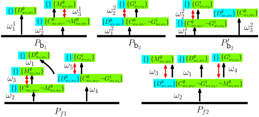
Figure 3: Illustrations of intermediate R-posets. $P_{\texttt{b}_{1}}$ is the R-poset of $\varphi_{\texttt{b}_{1}}$; $P_{\texttt{b}_{2}},P^{\prime}_{\texttt{b}_{2}}$ are the R-posets of$\varphi_{\texttt{b}_{2}}$. $P_{\texttt{b}_{1}}\otimes P_{\texttt{b}_{2}}=\{P_{f1},P_{f2}\}$.

To begin with, the R-posets of $\varphi_{\texttt{b}_{1}}$ and $\varphi_{\texttt{b}_{2}}$ are computed as $\{P_{\texttt{b}_{1}}\},\{P_{\texttt{b}_{2}},P^{\prime}_{\texttt{b}_{2}}\}$, showed in Fig. 3. The subtask $\omega_{i}$ consists of a part (in blue) representing the self-loop labels $\sigma^{s}_{i}$ and a part (in green) representing the action labels $\sigma_{i}$. The directed black arrows represent the $\preceq$ relation and the bidirectional red arrows for the $\neq$ relation. $P_{\texttt{b}_{2}}$ is chosen first to compute the product $P_{\texttt{b}_{1}}\otimes P_{\texttt{b}_{2}}$, as it has less subtasks and ordering constraints compared with $P^{\prime}_{\texttt{b}_{2}}$. $P_{f1},P_{f2}$ are the results of $P_{\texttt{b}_{1}}\otimes P_{\texttt{b}_{2}}$ showed in Fig. 3. We choose $P_{f2}$ for the next iteration instead of $P_{f1}$ for the same reason as $P_{\texttt{b}_{2}}$. More specifically, there are two subtasks $\omega^{1}_{2}\in P_{\texttt{b}_{1}}$ and $\omega^{2}_{1}\in P_{\texttt{b}_{2}}$ with the same requirement $C^{\emptyset}_{w_{7},w_{7}}$ in the action labels, where their self-loop constraints have no conflicts. Thus, we can choose $\omega_{2}\in P_{f2}$ which satisfies both $\omega^{1}_{2}\in P_{\texttt{b}_{1}}$ and $\omega^{2}_{1}\in P_{\texttt{b}_{2}}$ with a mapping function $M(\omega^{2}_{1})=\omega_{2},M(\omega^{2}_{2})=\omega_{4}$, generated from Line 1 in Alg. 1. Otherwise, we can keep these two tasks and as Line 1 in Alg. 1. This case is shown in $P_{f1}$ with the mapping function $M(\omega^{2}_{1})=\omega_{4},M(\omega^{2}_{2})=\omega_{5}$. Moreover, the conflicts between the self-loop labels $\sigma^{s}_{i}$ and the task labels $\sigma_{j}$ are checked in Line 1. Consequently, $(\omega_{2},\omega_{1})$ is added to $\preceq$ without conflicts between $\sigma_{1}$ and $\sigma^{s}_{2}$. As shown in Fig. 4 showed, the final R-poset consists of $21$ subtasks generated offline and $12$ contingent subtasks added online. The length of the task formula $\varphi$ is $33$. The first R-poset is computed in $3.5s$ but the complete R-posets is not exhausted even after $11h$ of computation. This signifies the importance of an anytime algorithm to compute the R-posets.

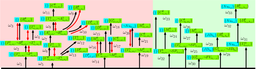
Figure 4: The final R-poset $P_{final}$ after the completion of all tasks.

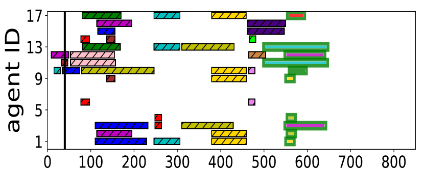
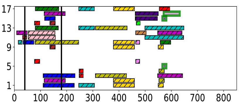
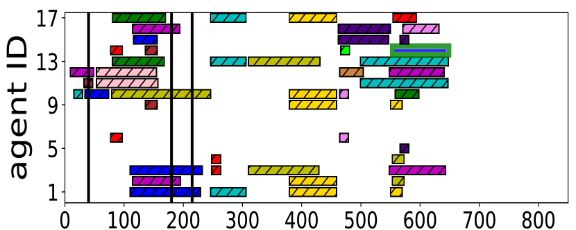
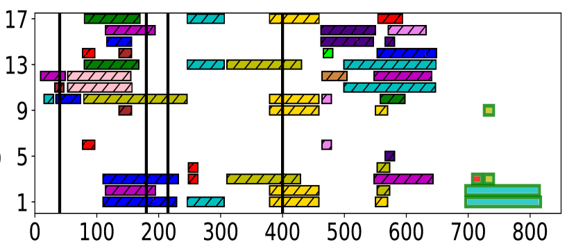
Figure 5: The Gantt graphs during the task execution. The black lines indicate that the additional tasks are added at $40s,180s,215s,400s$, and the green blocks represent contingent tasks added online.

During the task assignment and execution, there exists $5$ objects in $\mathcal{O}_{in}$, and then $5$ additional objects are added in $\mathcal{O}_{on}$ at $4$ different time instances as highlighted in the gantt graph of the complete system in Fig. 5. It can bee seen that all subtasks follow the specified ordering constraints in the R-posets. For instances, although the agents $6,14$ have arrived region $w7$ earlier than $100s$ for their first subtask $\sigma_{16}=\{M^{\emptyset}_{w7,w7}\}$ (in blue), they have to wait until that the subtask $\sigma_{14}=\{C^{\emptyset}_{w7,w7}\}$ has been fulfilled by agent $10$ (in brown), due to the constraints that $(\omega_{14},\omega_{16})\in\preceq,\{\omega_{14},\omega_{16}\}\in\neq$. It is worth noting that task $\omega_{7}$ (in green) cannot be executed at $380s$ before subtask $\omega_{6}$ (in purple) is finished as the required object $3$ has not been transferred to region $o_{4}$. Furthermore, most tasks are executed in parallel without much constraints for efficiency. Comparing to sequential execution, our method can reduce the completion time from $2013.5s$ to $815s$.

After execution, the complete formula $\varphi$ has a length of $62$, which can not be converted to NBA within $5h$. Instead, our algorithm of online adaptation is triggered $4$ times, which takes $10.96s$ in total. In contrast, to compute the products offline will take $32.47s$. The trajectories of agents are shown in Fig. 1 as gray lines while the trajectories for objects are shown in red. It is worth noting that the paths respect both the environment and temporal constraints. For instance, region $h_{13}$ is in shadow and agents of type $Nu$ can not enter due to the label constraints $\neg Nu_{h_{13}}$. Moreover, the $Transfer$ behavior is collaborative and requires two agents with $carry$ function to move an object of type $SP$ to the target region. Thus, the regions $o_{1},o_{2},o_{3}$ are forbidden during the execution of $Transfer$, due to the constraints $\bigwedge_{\ell=1\cdots 3}\neg SP$ caused by the newly-added object $SP$.

V-C Hardware Experiment

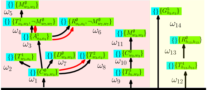
Figure 6: Final R-poset $P_{final}$ in the hardware experiment.

We further test the proposed method on hardware within a simplified hospital environment. The multi-agent system consists of $10$ differential drive mobile robots, with 3 $JD$ in green, 3 $SD$ in yellow and 4 $Nu$ in blue. The basic formulas in $\varPhi_{b}$ are given by: $\varphi_{\texttt{b}_{1}}=\Diamond(C^{\emptyset}_{w3,w3}\land\Diamond(T^{1}_{w3,o4}\land\Diamond(A^{1}_{o4,o4}\land\neg R^{1}_{o4,o4}\land\Diamond(T^{1}_{o4,w3}\land\neg A^{1}_{o4,o4}\land\Diamond C^{\emptyset}_{w3,w3}))\land\Diamond R^{\emptyset}_{o4,o4}));$ $\varphi_{\texttt{b}_{2}}=\Diamond(C^{\emptyset}_{w3,w3}\land\neg T^{2}_{w3,e2}\land\Diamond D^{\emptyset}_{w3,w3}\land\Diamond T^{2}_{w3,e2});$ $\varphi_{\texttt{b}_{3}}=\Diamond(T^{3}_{h5,w2}\land\Diamond C^{\emptyset}_{w2,w2}\land\Diamond M^{\emptyset}_{w2,w2});$ $\varphi_{\texttt{b}_{4}}=\neg M^{\emptyset}_{w2,w2}\textsf{U}C^{\emptyset}_{w2,w2}$.

As shown in Fig. 6, the final R-poset consists of $14$ subtasks of which the part in red background is calculated offline, while the part in yellow is generated online. Subtask $\omega_{1}$ is generated by Line 1 in Alg. 1 as the first $C^{\emptyset}_{w3,w3}$ of $\varphi_{\texttt{b}_{1}}$ and the $C^{\emptyset}_{w3,w3}$ of $\varphi_{\texttt{b}_{2}}$. A new partial relation is added via Line 1 due to the conflicts between $\neg M^{\emptyset}_{w2,w2}$ in $\varphi_{\texttt{b}_{4}}$ and the $M^{\emptyset}_{w_{2},w_{2}}$ in $\varphi_{\texttt{b}_{3}}$. The complete R-poset product is derived in $3.1s$ while the task assignment takes $2.7s$ in average. As shown in Fig. 7, the Gantt graph is updated twice at $5s$ and $100s$ during execution. The proposed TDCN method in Alg. 2 generates a complete assignment based on the given model. However, the movement of agents during real execution requires more time due to drifting and collision avoidance. Nonetheless, the proposed method can adapt to these fluctuations and still satisfy the ordering constraints. The final agent and object trajectories are shown in Fig. 8. Simulation and experiment videos are provided in the supplementary files.

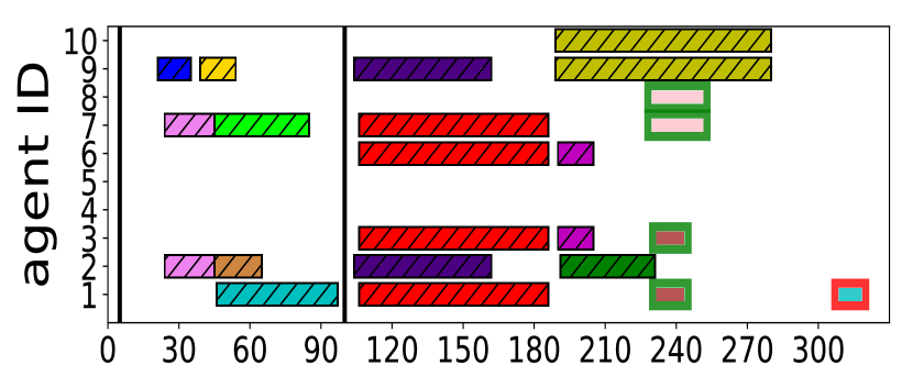
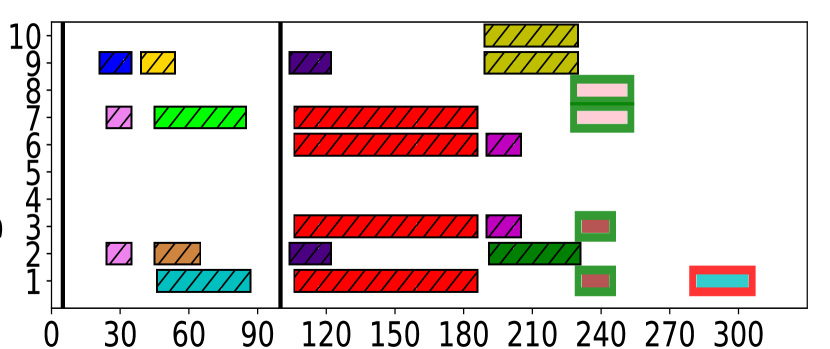
Figure 7: Gantt graph of task execution in the hardware experiment: the actual execution (Left) and the planned execution (Right).

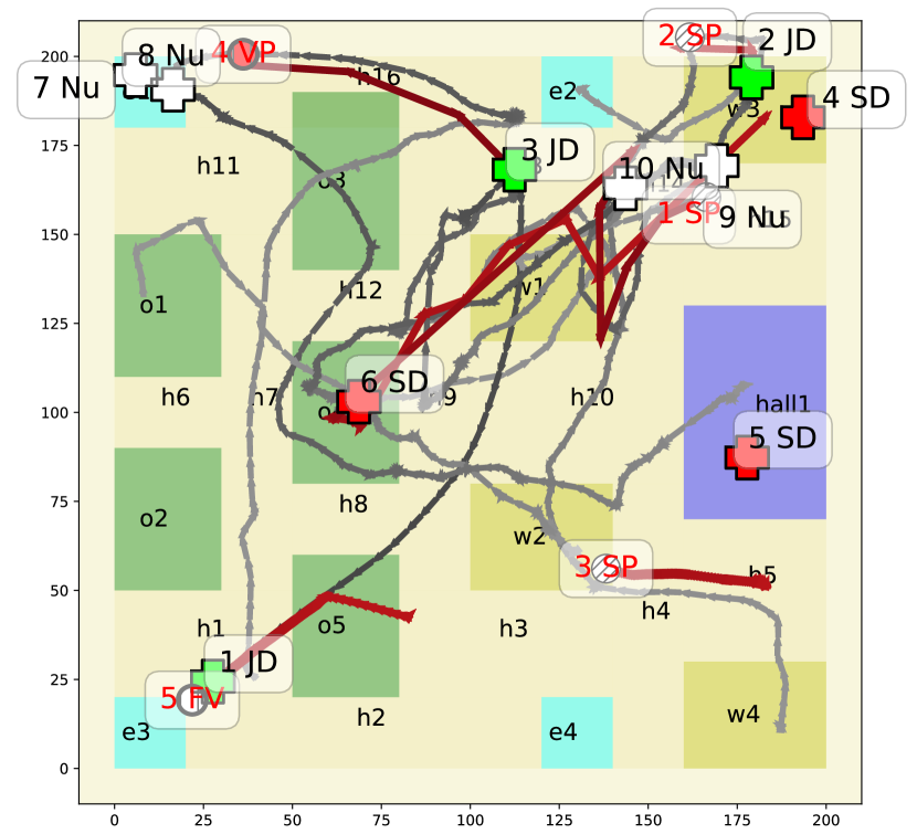
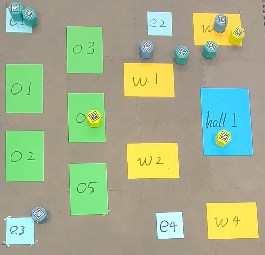
Figure 8: Trajectories of agents in grey and objects in red (Left); a snapshot during execution (Right).

V-D Scalability Analysis

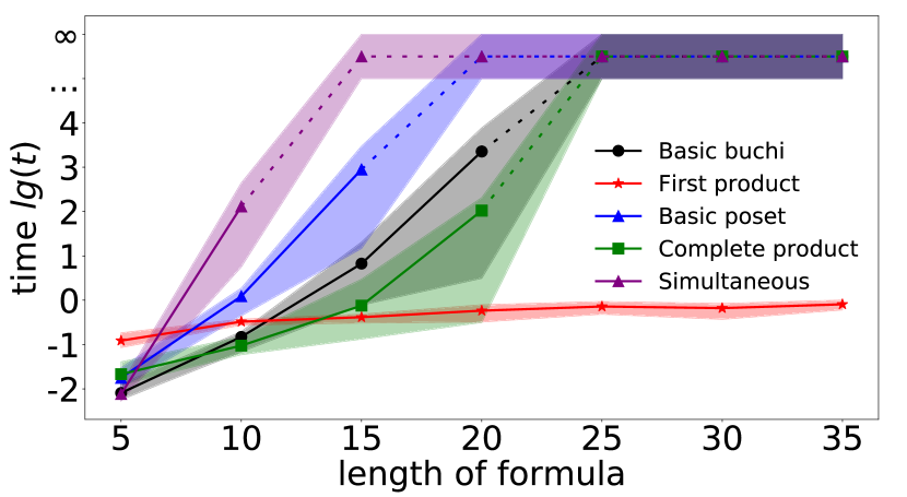
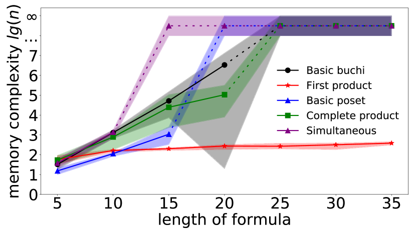
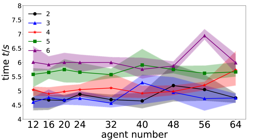
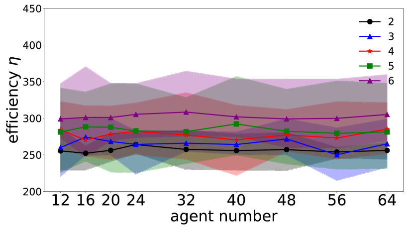
Figure 9: The computation complexity (Upper Left) and memory complexity (Upper Right); The computation time (Lower Left) and execution efficiency (Lower Right) with different number of agents and objects.

To further validate the scalability of the proposed method against existing methods, we evaluate the time and memory complexity for computation both first R-poset and complete R-posets, given a set of task formulas with lengths between $5$ to $40$. All conversions from the LTL formula to NBA is via LTL2BA, against four baselines: (i) the direct translation; (ii) the first R-poset by products; (iii) the complete R-posets by [3]; (iv) the complete R-posets by products; (v) the decomposition algorithm from [20]. As shown in Fig. 9, the computation time and memory both increase quickly with the length of formulas. Most algorithms run out of memory or time when the length exceeds $20$. In comparison, our method can always generate the first valid R-poset in a short time, although the complete product is also infeasible for formulas with length more than $25$. It is consistent with our complexity analysis in Sec. IV-E. Moreover, the computation time is recorded for different number of agents and objects. As shown in Fig. 9, the computation time only increases slightly as the number of agents systems while the number of objects has a larger impact (all under $7s$). This indicates that the proposed assignment algorithm scales well with the system size.

VI Conclusion

In this letter, a new task planning method is proposed for multi-agent system under LTL tasks, to tackle the computational complexity for long and complex task formulas. The direct translation of the complete task formula into the associated NBA is avoided, by instead computing R-posets and their products. The task assignment algorithm can ensure the temporal and collaborative constraints within the R-posets. The proposed methods scale well to long task formulas that are generated online and large system sizes.

References

- [1] Katoen and Joost-Pieter, Principles of model checking. Principles of model checking, 2008.
- [2] C. K. Verginis, Y. Kantaros, and D. V. Dimarogonas, “Planning and control of multi-robot-object systems under temporal logic tasks and uncertain dynamics,” arXiv preprint arXiv:2204.11783, 2022.
- [3] Z. Liu, M. Guo, and Z. Li, “Time minimization and online synchronization for multi-agent systems under collaborative temporal tasks,” arXiv preprint arXiv:2208.07756, 2022.
- [4] P. Schillinger, M. Bürger, and D. V. Dimarogonas, “Simultaneous task allocation and planning for temporal logic goals in heterogeneous multi-robot systems,” The international journal of robotics research, vol. 37, no. 7, pp. 818–838, 2018.
- [5] M. Ben-Ari, “A primer on model checking,” ACM Inroads, vol. 1, no. 1, pp. 40–47, 2010.
- [6] P. Gastin and D. Oddoux, “Fast ltl to büchi automata translation,” in Computer Aided Verification, G. Berry, H. Comon, and A. Finkel, Eds. Berlin, Heidelberg: Springer Berlin Heidelberg, 2001, pp. 53–65.
- [7] X. Ding, S. L. Smith, C. Belta, and D. Rus, “Optimal control of markov decision processes with linear temporal logic constraints,” IEEE Transactions on Automatic Control, vol. 59, no. 5, pp. 1244–1257, 2014.
- [8] M. Kloetzer and C. Mahulea, “Accomplish multi-robot tasks via petri net models,” in 2015 IEEE International Conference on Automation Science and Engineering (CASE), 2015, pp. 304–309.
- [9] K. Leahy, Z. Serlin, C.-I. Vasile, A. Schoer, A. M. Jones, R. Tron, and C. Belta, “Scalable and robust algorithms for task-based coordination from high-level specifications (scratches),” IEEE Transactions on Robotics, vol. 38, no. 4, pp. 2516–2535, 2022.
- [10] P. Schillinger, M. Bürger, and D. V. Dimarogonas, “Hierarchical ltl-task mdps for multi-agent coordination through auctioning and learning,” The international journal of robotics research, 2019.
- [11] Y. Kantaros and M. M. Zavlanos, “A temporal logic optimal controlsynthesis algorithm for large-scale multi-robot systems,” The International Journal of Robotics Research, vol. 39, no. 7, p. 027836492091392, 2020.
- [12] N. Piterman, A. Pnueli, and Y. Sa’ar, “Synthesis of reactive(1) designs,” in Verification, Model Checking, and Abstract Interpretation, E. A. Emerson and K. S. Namjoshi, Eds. Berlin, Heidelberg: Springer Berlin Heidelberg, 2006, pp. 364–380.
- [13] V. Vasilopoulos, Y. Kantaros, G. J. Pappas, and D. E. Koditschek, “Reactive planning for mobile manipulation tasks in unexplored semantic environments,” in International Conference on Robotics and Automation, 2021.
- [14] C. K. Verginis and D. V. Dimarogonas, “Multi-agent motion planning and object transportation under high level goals,” in IFAC World Congress, 2018.
- [15] B. Lacerda, D. Parker, and N. Hawes, “Optimal and dynamic planning for markov decision processes with co-safe ltl specifications,” in 2014 IEEE/RSJ International Conference on Intelligent Robots and Systems, 2014, pp. 1511–1516.
- [16] S. Feyzabadi and S. Carpin, “Multi-objective planning with multiple high level task specifications,” in 2016 IEEE International Conference on Robotics and Automation (ICRA), 2016, pp. 5483–5490.
- [17] C. Belta, B. Yordanov, and E. A. Gol, Formal methods for discrete-time dynamical systems. Springer, 2017, vol. 15.
- [18] X. Luo and M. M. Zavlanos, “Temporal logic task allocation in heterogeneous multirobot systems,” IEEE Transactions on Robotics, vol. 38, no. 6, pp. 3602–3621, 2022.
- [19] Smith, “The contract net protocol: High-level communication and control in a distributed problem solver,” IEEE Transactions on Computers, vol. C-29, no. 12, pp. 1104–1113, 1980.
- [20] F. Faruq, D. Parker, B. Laccrda, and N. Hawes, “Simultaneous task allocation and planning under uncertainty,” in 2018 IEEE/RSJ International Conference on Intelligent Robots and Systems (IROS). IEEE, 2018, pp. 3559–3564.