Studying X-ray spectra from large-scale jets of FR II radio galaxies: application of shear particle acceleration

Abstract

Shear particle acceleration is a promising candidate for the origin of extended high-energy emission in extra-galactic jets. In this paper, we explore the applicability of a shear model to 24 X-ray knots in the large-scale jets of FR II radio galaxies, and study the jet properties by modeling the multi-wavelength spectral energy distributions (SEDs) in a leptonic framework including synchrotron and inverse Compton - CMB processes. In order to improve spectral modelling, we analyze Fermi-LAT  data for five sources and reanalyze archival data of Chandra on 15 knots, exploring the radio to X-ray connection. We show that the X-ray SEDs of these knots can be satisfactorily modelled by synchrotron radiation from a second, shear-accelerated electron population reaching multi-TeV energies. The inferred flow speeds are compatible with large-scale jets being mildly relativistic. We explore two different shear flow profiles (i.e., linearly decreasing and power-law) and find that the required spine speeds differ only slightly, supporting the notion that for higher flow speeds the variations in particle spectral indices are less dependent on the presumed velocity profile. The derived magnetic field strengths are in the range of a few to ten microGauss, and the required power in non-thermal particles typically well below the Eddington constraint. Finally, the inferred parameters are used to constrain the potential of FR II jets as possible UHECR accelerators.

1 Introduction

Radio galaxies are characterized by the large-scale radio emission on scales from kiloparsec (kpc) to megaparsec (Mpc) energized by the jets launched from their active galactic nuclei (AGNs). Based on their observational morphology, they are divided into low-power Fanaroff-Riley type I (FR I) sources and high-power Fanaroff-Riley type II (FR II) sources (Fanaroff & Riley, 1974). Kpc-scale jets in radio galaxies have been studied for several decades. Their multi-wavelength images at radio, optical, and X-ray wavelengths commonly consist of bright knots (Kraft et al., 2002; Clautice et al., 2016; Hardcastle et al., 2016). The radio and optical emission from kpc-scale jets are considered to be produced by synchrotron radiation of electrons, however the origin of the extended X-ray emission is still unclear (Harris & Krawczynski, 2006).

For most knots in FR I jets, the radio, optical, and X-ray spectrum can typically be explained by synchrotron radiation from a single population of electrons (e.g. Perlman et al., 2001; Hardcastle et al., 2001; Sun et al., 2018). The detection of the extended TeV emission from the kpc-scale jet of Centaurus A by the High Energy Stereoscopic System (H.E.S.S.) also supports the synchrotron origin of the X-rays emission (H. E. S. S. Collaboration et al., 2020). On the other hand, in FR II jets the X-ray emission can exhibit much harder spectra than seen in the radio to optical band, which can not be modeled by the synchrotron radiation from a single population of electrons (e.g. Jester et al., 2006, 2007). It has been proposed that such extended X-ray emission could be produced by inverse Compton up-scattering (IC) of cosmic microwave background (IC/CMB) photons (Georganopoulos & Kazanas, 2003; Abdo et al., 2010; McKeough et al., 2016; Wu et al., 2017; Guo et al., 2018; Zhang et al., 2018b), although a large jet (bulk) Lorentz factor $\Gamma$ would then be required on kpc-scales (e.g. Tavecchio et al., 2000; Celotti et al., 2001; Zhang et al., 2010; Zhang et al., 2018a). However, this scenario is challenged by recent polarimetry observations and $\gamma$-ray observations (see also Georganopoulos et al., 2016, for a review), e.g. in the jets of 3C 273 (Perlman et al., 2020; Meyer & Georganopoulos, 2014), PKS 0637-752 (Perlman et al., 2020; Breiding et al., 2023), and PKS 1136-135 (Cara et al., 2013; Breiding et al., 2023). In an alternative scenario, the hard X-ray spectra could be related to the synchrotron radiation of a second electron population that is different from the radio-optical emission (e.g., Jester et al., 2006; Zhang et al., 2009; Georganopoulos et al., 2016; Sun et al., 2018), or to the synchrotron radiation of protons in the extended regions of large-scale jets (Aharonian, 2002; Kundu & Gupta, 2014).

A synchrotron origin of X-rays emission requires $\sim 100$ TeV electrons, which will cool on a timescale of a few thousand years in a typical magnetic field strength of $\sim 10\leavevmode\nobreak\ \mu$G. This corresponds to a distance of several hundred pc. Thus for jet knots of sizes larger than 1 kpc, a distributed (re)acceleration mechanism is required to maintain the diffuse X-ray emission in the knots. Shear acceleration is a promising candidate mechanism for this (Liu et al., 2017; Rieger, 2019; Wang et al., 2021; Tavecchio, 2021). In shearing flows, particles can gain energy by elastically scattering off small-scale magnetic field inhomogeneities embedded in velocity-shearing layers. The process can in principle be understood as a Fermi-type particle acceleration mechanism (Rieger & Duffy, 2004; Rieger et al., 2007; Liu et al., 2017; Lemoine, 2019; Rieger, 2019). The accelerated particle spectra and achievable maximum energies have been extensively studied, and found to be mainly depending on the velocity profile and turbulence spectrum (e.g. Liu et al., 2017; Webb et al., 2018, 2019, 2020; Rieger & Duffy, 2019, 2021, 2022; Wang et al., 2021, 2023). Velocity-shearing flows are naturally expected in AGN jets. For example, high-resolution radio imaging and polarization studies have indicated the presence of velocity gradients transverse to the main jet axes in FR II jets (e.g., Boccardi et al., 2016; Nagai et al., 2014). In general, interaction of a jet with its environment is likely to excite instabilities and introduce velocity shearing. In fact, our recent 3D relativistic magneto-hydrodynamic simulations have shown that shearing layers can be naturally self-generated by a relativistic jet spine interacting with its surrounding medium (Wang et al., 2023).

In a previous paper, we have obtained an exact solution for the steady-state particle spectrum within a Fokker-Planck approach, and used it to successfully reconstruct the observed, diffuse X-ray emission in two exemplary sources: the kpc-scale jet in Cen A (FR I type), and the knots A+B1 and C2 in the jet of 3C 273 (FR II type) (Wang et al., 2021). In this paper, we further explore the application of such a shear acceleration model to a large-sample of X-ray knots in FR II type jets, and study the jet properties by modeling their multi-wavelength data. In Section 2, we describe the details of the data analysis process and show spectral properties for the X-ray and $\gamma$-ray spectrum. In Section 3, we describe the SED modelling in the framework of shear acceleration. In Section 4, we present the fitting results with this shear acceleration model and discuss their implications. The conclusions are given in Section 5.

2 Data

We select a sample of eight FR II radio galaxies with clear morphology and wavelength coverage in the data-set of radio-to-X-ray data from the X-ray jet catalog and the paper Zhang et al. (2018a), including 3C 273, 3C 403, 3C 17, Pictor A, 3C 111, PKS 2152-699, 3C 353, and S5 2007+777. The details of the sources are shown in the following.

3C 273: 3C 273 is an ideal FR II radio galaxy with rich multi-wavelength observations. The origin of the hard X-ray emission from its knots has been actively debated (Jester et al., 2005, 2006; Uchiyama et al., 2006; Jester et al., 2007; Zhang et al., 2010; Zhang et al., 2018a; Wang et al., 2020). It is known to host a super-massive black hole (SMBH) of mass of $\sim 6.6\times 10^{9}\mbox{$\rm M_{\odot}$}$ (Paltani & Türler, 2005), $\rm M_{\odot}$ is the mass of sun. The redshift is z = 0.158, such that $1\arcsec$ corresponds to 2.7 kpc (Sambruna et al., 2001). The jet is about $20\arcsec$ in Chandra observation, which indicates that the projected length of the jet can extend over 50 kpc. Proper-motion studies provide an upper-limit on the velocity $(\Gamma<2.9)$ and a viewing angle of $\theta\sim$ $7\hbox{${}^{\circ}$}$ (Meyer et al., 2016). Marchenko et al. (2017) find that the prominent brightness enhancements in the X-ray and far-ultraviolet jet of 3C 273 can be resolved transversely as extended features with sizes of about 0.5 kpc. We select five X-ray regions, A, B1+B2, B3+C1, C2, and D1+D2H3 to perform the spectral analysis, and combine adjacent knots if they are difficult to distinguish. The radio and optical data are obtained from Jester et al. (2007), and the $\gamma$-ray data are taken from Meyer & Georganopoulos (2014).

3C 403: 3C 403 is one of the best examples of synchrotron X-ray emission from the jet of a powerful narrow-line radio galaxy (Kraft et al., 2005). The mass of its SMBH is $\sim 1.8\times 10^{8}\mbox{$\rm M_{\odot}$}$ as estimated from its K-band bulge luminosity (Vasudevan et al., 2010). According to the unified models of FR II radio galaxies, the jets of narrow-line radio galaxies are at a large viewing angle of $>45\hbox{${}^{\circ}$}$ (Kraft et al., 2005; Barthel, 1989). The east jet of 3C 403 includes two significant X-ray knots, F1 and F6. The measured redshift of the host galaxy is $z=0.059$, corresponding to a luminosity distance of 260.6 Mpc $(1\rm\arcsec=1.127\ kpc)$. The radio and optical data are taken from Kraft et al. (2005) and Werner et al. (2012).

3C 17: We select two X-ray knots (S3.7 and S11.3) in the powerful jet of the radio galaxy 3C 17. The mass of its SMBH is $\sim 5.0\times 10^{8}\mbox{$\rm M_{\odot}$}$ (Sikora et al., 2007). The measured redshift of the host galaxy ($z$ = 0.22) corresponds to a conversion scale of $1\rm\arcsec$ = 3.47 kpc. While we assume a synchrotron origin, we note that given the SED shape and unusual character of S11.3, it cannot be excluded that IC/CMB contributes to the emission from this knot (Massaro et al., 2009; Rahman et al., 2023).The radio, optical, and X-ray data are taken from Massaro et al. (2009).

Pictor A: Pictor A has an unilateral and straight jet in the radio and X-ray energy bands (Gentry et al., 2015). This source harbors a SMBH of mass $\sim 4.0\times 10^{7}\mbox{$\rm M_{\odot}$}$ (Ito et al., 2021). The measured redshift of the host galaxy is $z=0.0304$ $(1\rm\arcsec=0.697\ kpc$ (Hardcastle et al., 2016). Tingay et al. (2000) have estimated a viewing angle $\theta\lesssim 51\hbox{${}^{\circ}$}$ based on Very Long Baseline Array (VLBA) observations. We select three knots, HST-32, HST-106, and HST-112, with radio, optical, and X-ray data taken from Gentry et al. (2015).

3C 111: 3C 111 is a typical FR II radio galaxy with a SMBH of mass $\sim 2.0\times 10^{8}\mbox{$\rm M_{\odot}$}$ (Ito et al., 2021). It is located at a redshift of $z$ = 0.158, corresponding to a luminosity distance of 215 Mpc. Chandra observations by Clautice et al. (2016) report X-ray emission from three knots, K14, K30, and K61 in the northern jet. VLBA observations reveal an angle to the line of sight $\theta\lesssim 20\hbox{${}^{\circ}$}$ and a velocity $\sim$ 0.98 for the entire jet (Oh et al., 2015). The radio and optical data are taken from Clautice et al. (2016), and the $\gamma$-ray data are taken from Zhang et al. (2018a).

PKS 2152-699: PKS 2152-699 is a well-studied FR II radio galaxy at a redshift of $z$ = 0.0283, corresponding to a luminosity distance of 122 Mpc (Ly et al., 2005). This radio galaxy is one of the brightest sources in the southern sky at 2.7 GHz (Ly et al., 2005). Worrall et al. (2012) found a bright knot D about 10$\arcsec$ from the host galaxy and estimate a total time-averaged jet power $4\times 10^{44}\rm erg\ s^{-1}$. The radio and optical data for this knot are taken from Fosbury et al. (1998) and Worrall et al. (2012).

3C 353: The jet of 3C 353 has three significant X-ray knots, E23, E88, and W47 (Kataoka et al., 2008). Swain et al. (1998) estimate a rather large viewing angle of $60\hbox{${}^{\circ}$}<\theta<90\hbox{${}^{\circ}$}$ for the whole jet based on Very Large Array (VLA) observations at 8.4 GHz. The measured redshift of the host galaxy is $z=0.0304$, corresponding to a conversion scale of $1\rm\arcsec$ = 0.60 kpc (Kataoka et al., 2008). The radio, optical, and previous X-ray data are taken from Kataoka et al. (2008).

S5 2007+777: The X-ray jet of S5 2007+777 exhibits properties of both FR I and FR II radio galaxies (Sambruna et al., 2008a). The jet has an angle of $<32\hbox{${}^{\circ}$}$ to the line of sight, and the deprojected jet length significantly exceeds 150 kpc (Sambruna et al., 2008b). The source harbors an SMBH of mass $\sim 2.5\times 10^{7}\mbox{$\rm M_{\odot}$}$ (Wu et al., 2002). The measured redshift of its host galaxy is $z=0.342$, corresponding to a conversion scale of $1\rm\arcsec$ = 4.80 kpc (Sambruna et al., 2008b). We select five X-ray knots, including K3.6, K5.2, K8.5, K11.1, and K15.9. The radio data and the optical upper limits are taken from Sambruna et al. (2008b), and the $\gamma$-ray data are taken from Mondal & Gupta (2019).

2.1 Chandra data analysis

The Chandra X-ray Observatory launched in 1999, provides high resolution ($<0.5\rm\arcsec$) X-ray imaging and spectroscopy in the energy range 0.1 – 10 keV (Weisskopf et al., 2002). The Science Instrument Module of Chandra has two focal plane instruments, the Advanced CCD Imaging Spectrometer (ACIS) and the High Resolution Camera (HRC). The ACIS module is used for spectral analysis. In this paper, the spectral extraction is performed using the CIAO (v4.13) software and the Chandra Calibration Database (CALDB, v4.9.4). The spectral analysis is performed using Sherpa tool.

The X-ray data of the jets in our sample are all from the Chandra X-ray Observatory. Owing to the accumulative exposure and the enhanced software tools of Chandra , we perform an improved analysis for five sources 3C 111, 3C 403, PKS 2152-699, S5 2007+777, and 3C 273 to derive more accurate spectrometric information. The observational information of the five FR II radio galaxies is shown in Table 5 (see the Appendix B). We analyze the Chandra ACIS data following the guidance of $Science$ $Threads$. In order to reduce the deviations caused by the position offsets of different observations, we perform astrometric corrections. The counts image, exposure map, and the weighted PSF map are produced by performing fluximage and mkpsfmap tools, respectively. We obtain the locations of target sources using the wavdetect tool. For observations with more than two times, we perform the cross-matching between the reference observation and the others; we use wcs_match to produce a transform matrix and wcs_update tool to update the coordinates of the shorter observation. We select the longest exposure observation as a reference.

For the spectral analysis, we perform aperture photometry using specextract on each knot. The locations of the selected regions, the corresponding length and width ($L_{\rm knot}$ and $W_{\rm knot}$) of the knot are listed in Table 6 (see the Appendix B), where $L_{\rm knot}$ is the half width at half maximum along the jet, $W_{\rm knot}$ is the half width at half maximum transverse to the jet. We use sherpa package to perform the broadband fitting of multi-observations simultaneously with a single power-law plus the Galactic absorption model. The flux of knots in our sample are extracted in the $0.3-7.0$ keV energy band. We keep the absorption column density $N_{\rm H}$  free, and we do not find evidence for significant deviation for all knots if $N_{\rm H}$  is kept frozen. The X-ray flux densities and reduced chi-square $\chi^{2}$ are listed in Table 1. The signals of X-ray radiation from some knots are too weak, leading $\chi^{2}$ to deviate from 1, and $N_{\rm H}$  hard to be constrained tightly. The errors of flux and photon index are calculated at 90% confidence level. When the spectral indices for some knots are not convergent due to too few photons, we set them to be 1.0. The spectral indices of the X-ray emission are typically in the range of $0.5-1.2$. The spectral index measurement for knot D1+D2H3 in 3C 273 is $1.20^{+0.27}_{-0.11}$. We note that Jester et al. (2006) obtained a somewhat harder X-ray spectrum between $1.02\pm{0.05}$ and $1.04\pm{0.04}$. The difference might partly be related to systematic effects from the corrections for ACIS contamination . Since $N_{\rm H}$  is kept free in our analysis, the error on the spectral index is larger. In general, the spectral indices do not reveal softening along the jet, which indicates that these FR II jets need an efficient distributed acceleration mechanism to explain the harder X-ray spectrum. Assuming a synchrotron origin of the FR II jet emission, the harder X-ray spectra and the differences between the spectral indices of $\alpha_{\rm RO}$ and $\alpha_{\rm OX}$ shown in Table 1 indeed suggest that the radiation from a single electron population cannot explain the radio to X-ray SED.

Table 1: The (re-analyzed) X-ray flux of the knots for different energy bands.

Source	Knot	$\nu F_{\nu}$a	$\nu F_{\nu}{\textsuperscript{b}}$	$\nu F_{\nu}$c	$N_{\rm H}$[$\rm\times 10^{22}/cm^{2}$]d	$\alpha_{\rm X}$ e	reduced $\chi^{2}$	$\alpha_{\rm RO}$	$\alpha_{\rm OX}$
3C 273	A	113$\pm$3.73	155$\pm$4.67	165$\pm$8.67	< 0.03	$0.84^{+0.17}_{-0.01}$	0.55	0.89$\pm$0.01	0.76$\pm$0.01
	B1+B2	84.1$\pm$5.74	102$\pm$6.02	109$\pm$9.68	$0.05\pm{0.03}$	$0.92\pm{0.09}$	0.74	0.95$\pm$0.01	0.81$\pm$0.02
	B3+C1	23.7$\pm$2.91	25.2$\pm$2.96	23.3$\pm$5.20	< 0.09	$1.02^{+0.37}_{-0.17}$	0.42	0.92$\pm$0.01	1.05$\pm$0.03
	C2	24.9$\pm$3.15	29.4$\pm$3.54	30.1$\pm$3.81	< 0.02	$0.94^{+0.15}_{-0.11}$	0.49	0.97$\pm$0.01	1.00$\pm$0.02
	D1+D2H3	54.4$\pm$9.33	49.1$\pm$7.74	39.7$\pm$8.86	< 0.11	$1.20^{+0.27}_{-0.11}$	0.57	1.00$\pm$0.01	1.13$\pm$0.01
3C 403	F1	1.27$\pm$0.43	4.52$\pm$0.76	5.83$\pm$2.86	< 0.86	1.00	0.99	0.58$\pm$0.01	$1.16^{+0.04}_{-0.05}$
	F6	5.80$\pm$0.94	6.07$\pm$0.70	6.37$\pm$1.79	< 0.52	$0.96^{+1.46}_{-0.71}$	1.08	0.71$\pm$0.01	1.17$\pm$0.02
3C 111	K14	3.27$\pm$0.91	9.51$\pm$2.69	32.6$\pm$14.4	$0.58^{+0.56}_{-0.41}$	$0.47^{+0.40}_{-0.38}$	0.45	0.74$\pm$0.01	$0.96^{+0.04}_{-0.06}$
	K30	5.20$\pm$2.02	6.50$\pm$2.65	9.63$\pm$4.33	< $0.95$	$0.72^{+0.79}_{-0.53}$	0.33	0.73$\pm$0.01	$0.89^{+0.05}_{-0.07}$
	K61	14.4$\pm$2.31	15.0$\pm$1.98	16.0$\pm$3.19	$0.77^{+0.51}_{-0.37}$	$0.95^{+0.48}_{-0.44}$	0.53	$1.00^{+0.02}_{-0.03}$	$0.81^{+0.06}_{-0.05}$
PKS 2152-699	D	6.74$\pm$1.67	5.37$\pm$0.99	5.26$\pm$2.53	< 0.29	$1.22^{+0.89}_{-0.42}$	0.29	1.23$\pm$0.01	1.09$\pm$0.03
S5 2007+777	K3.6	0.56$\pm$0.38	1.44$\pm$0.79	< 18.0	< 1.13	1.00	0.50	0.84$\pm$0.02	-
	K5.2	0.71$\pm$0.45	1.90$\pm$0.95	< 15.8	-	1.00	0.99	1.10$\pm$0.02	-
	K8.5	2.68$\pm$0.61	5.19$\pm$0.91	9.76$\pm$3.76	< 0.56	$0.94^{+1.14}_{-0.62}$	0.45	0.72$\pm$0.01	-
	K11.1	0.61$\pm$0.34	1.35$\pm$0.74	< 10.5	< 24.4	1.00	0.40	0.73$\pm$0.02	-
	K15.9	1.68$\pm$0.63	1.77$\pm$0.54	2.22$\pm$1.51	< 9.88	1.00	0.30	0.95$\pm$0.02	-

• Flux in energy range of $0.3-0.8$ keV.

• Flux in energy range of $0.8-2.5$ keV.

• Flux in energy range of $2.5-7.0$ keV.

• Hydrogen-absorbing column density.

• For some knots, the photon counts are not high enough to constrain the index, in which case they are set to be 1.
  Spectral index $\alpha$ and flux are expressed as $F_{\nu}\propto\nu^{-\alpha}$, $\nu$ denotes the frequency. The errors of the flux, $N_{\rm H}$, and $\alpha_{\rm X}$ are calculated at a 90% confidence level. The errors of $\alpha_{\rm RO}$ and $\alpha_{\rm OX}$ are calculated based on the error bars in their corresponding references.

Table 2: The $\gamma$-ray flux of the knots.

Source	Time interval (MET )	$\nu F_{\nu}$a	$\nu F_{\nu}{\textsuperscript{b}}$	$\nu F_{\nu}$c
Pictor A	239557417 - 668590613	10.4$\pm$0.51	3.87$\pm$0.07	2.87$\pm$0.71
3C 17	239557417 - 668305234	7.00$\pm$0.02	1.21$\pm$0.57	-
PKS 2152-699	239557417 - 668305234	7.00$\pm$0.31	1.11$\pm$0.67	-
3C 403	239557417 - 668631991	< 0.70	-	-
3C 353	239557417 - 668933761	< 0.50	-	-

• Flux in the energy range of $0.5-1.3$ GeV.

• Flux in the energy range of $1.3-3.7$ GeV.

• Flux in the energy range of $3.7-10$ GeV.
  MET denotes the Mission Elapsed Time.
  The upper limits are computed at $99\%$ confidence level ($3\sigma$).

2.2 Fermi-LAT data analysis

The Fermi Large Area Telescope (Fermi-LAT), launched in 2008, is a wide field-of-view imaging $\gamma$-ray telescope covering the energy range from about 20 MeV to more than 300 GeV (Atwood et al., 2009). We select Fermi-LAT Pass 8 data around the sources 3C 17, 3C 353, 3C 403, Pictor A, and PKS 2152-699 regions. The observation time is listed in Table 2. We use a 10^∘$\times$10^∘ square region centered at the position of target sources as the region of interest. We process the data through the current Fermitools from conda distribution together with the latest version of the instrument response function P8R3_SOURCE_V3. We select the "source" event class in an energy range from $0.5-10$ GeV for individual source analysis. Both the front and back converted photons are included. To exclude time periods when some spacecraft event affected the data quality, we use the recommended expression (DATA_QUAL > 0) && (LAT_CONFIG == 1). To reduce the background contamination from the earth’s albedo, only the events with zenith angles less than 90^∘ are included. We apply the Python module that implements a maximum likelihood optimization technique for a standard binned analysis . In the background model, we include the sources in the Fermi-LAT ten-year catalog (4FGL-DR2, Ballet et al., 2020). We use the script make4FGLxml.py to generate the source model files, and the parameters for the target sources within 9.0^∘of the center are set free. For the diffuse background components, we use the latest Galactic diffuse emission model gll_iem_v07.fits and isotropic extragalactic emission model iso_P8R3_SOURCE_V3_v1.txt with their normalization parameters free. We assume the target source is a point-like source and has a power-law spectrum. To derive the SED, we divided the energy interval into three equal bins in logarithmic space and performed the maximum likelihood fitting in each energy bin. For 3C 353 and 3C 403, where the signals are detected with a significance of less than $2\sigma$, we calculated the upper limits within $3\sigma$ confidence level. The derived flux calculated within $3\sigma$ confidence level is listed in Table 2, and the SEDs are shown in Figure LABEL:fig:2.

3 SED modeling and fitting

In our shear acceleration model, the radio-to-X-ray data is explained by synchrotron radiation from two populations of electrons (Wang et al., 2021). The low-energy electron population is responsible for the radio to optical emission, and might be related to first-order shock or second-order Fermi acceleration processes (e.g., Rieger et al., 2007; Liu et al., 2017; Tavecchio, 2021). The high-energy electron population is responsible for the UV-to-X-ray observation, and thought to be related to shear acceleration.

For simplicity we assume the low-energy population to have an exponential-cutoff power-law shape at $E\geq E_{\rm min1}$,

$$N_{1}(E)=A_{\rm 1}\left(\frac{E}{E_{0}}\right)^{-\alpha_{\rm 1}}\exp\left[-\left(\frac{E}{E_{\rm cutoff1}}\right)^{2}\right],$$ (1)

where $A_{1}$ is the normalization constant, $\alpha_{\rm 1}$ denotes the spectral index of the low-energy electrons, $E_{\rm cutoff1}$ is the cut-off energy and $E_{0}$ is set equal to 1 TeV, $E_{\rm min1}$ is the minimum energy of the low-energy electron. We note that the corresponding exponential shape might be obtained if diffusion of these electrons proceeds in the Bohm regime (e.g., Zirakashvili & Aharonian, 2007).

For the shear-accelerated high-energy population, we adopt the exact solution of the steady-state Fokker-Planck-type equation at $E\geq E_{\rm min2}$ (Wang et al., 2021),

$$N_{2}(E)=A_{+}E^{-\alpha_{+}}F_{+}(E,q)+A_{-}E^{-\alpha_{-}}F_{-}(E,q)\,.$$ (2)

The power-law spectral indices are given by

$$\alpha_{\pm}={1-q\over 2}\mp\sqrt{{(5-q)^{2}\over 4}+w},$$ (3)

where the $\alpha_{-}$ component dominates the particle spectrum. $w$ is a dimensionless measure of the shear viscosity, while $q$ denotes the power-law index of the turbulent spectrum. Here we adopt a Kolmogorov-type turbulence spectrum ($q=5/3$), which is in general consistent with numerical simulations (Wang et al., 2023). The functions $F_{\pm}(E,q)$ are defined as

$$F_{\pm}(E,q)={{}_{1}F_{1}}\left[{2-\alpha_{\pm}\over q-1},{2\alpha_{\pm}\over 1-q};-{6-q\over q-1}\left(\frac{E}{E_{\rm e,max}}\right)^{q-1}\right],$$ (4)

where $E_{\rm e,max}$ is the cut-off energy, and ${}_{1}F_{1}$ denotes the Kummer’s confluent hyper-geometric function (Abramowitz & Stegun, 1972). The integration constants $A_{\rm\pm}$ can be obtained by the condition $N_{2}(E)\to 0$ at $E\to\infty$ and the normalization of the spectrum.

In general, particle acceleration in shearing flows depends on the underlying flow velocity profile. Here we explore two different velocity profiles: For a linearly decreasing profile with $\beta(r)=\beta_{\rm 0,l}[1-(r/R_{\rm jet})]$, the shear viscosity $w$ can be expressed as (Wang et al., 2023),

$$w_{l}=\frac{10\beta_{\rm 0,l}^{2}}{[\zeta\ln(1-\beta_{\rm 0,l}^{2})+2\beta_{\rm 0,l}\rm tanh^{-1}(\beta_{\rm 0,l})]^{2}}.$$ (5)

where $\beta_{\rm 0,l}$ is the velocity on the jet axis, and $\zeta=W_{\rm sh}/R_{\rm jet}$, is $\sim$ 1/2 for FR II jets following the simulation result, here $R_{\rm jet}$ = $W_{\rm knot}$ denotes the jet radius, and $W_{\rm sh}$ is the width of the shearing region.

For a power-law type velocity profile with $\beta(r)=\beta_{\rm 0,p}/[1+(5r/R_{\rm jet})^{2}]$, where $\beta_{\rm 0,p}$ denotes the spine velocity, $w$ is of the form (Rieger & Duffy, 2022),

$$w_{p}=\frac{(6-q)t_{\rm acc}}{t_{\rm esc}}=116\langle\beta\rangle\ln^{-2}{(1+\Delta\beta)\over(1-\Delta\beta)},$$ (6)

where $\Delta\beta=(\beta_{\rm 0,p}-\beta(R_{\rm jet}))/(1-\beta_{\rm 0,p}\beta(R_{\rm jet}))$ is the relativistic relative velocity, $t_{\rm acc}$ and $t_{\rm esc}$ are the accelerating and the escaping time, respectively, and $\langle\beta\rangle\equiv\textstyle\int_{0}^{R_{\rm jet}}\beta(r)dr/\textstyle\int_{0}^{R_{\rm jet}}dr$ < 1 is a weighted, spatial average of the considered velocity profile. As $\beta_{\rm 0,l}$ and $\beta_{\rm 0,p}$ approach the speed of light ($\beta\rightarrow 1$), one obtains $w$ → 0, and the spectral index becomes $\alpha_{\rm-}=3-q=\frac{4}{3}$, which implies that in a jet with ultra-relativistic velocity, the spectral index of the accelerated electrons $\alpha_{-}$ becomes independent of the shape of the velocity profile (Webb et al., 2018, 2019; Rieger & Duffy, 2019, 2022).

To ensure that electrons can be effectively accelerated, two requirements need to be satisfied: (1) The scattering time is smaller than the acceleration time; (2) the acceleration time is smaller than the cooling time. Combining these two requirements, the corresponding cut-off energy of electrons and the resultant maximum energy of synchrotron photons can be expressed as (Wang et al., 2021),

$$E_{\rm e,{max}}=0.7B_{1}^{-2}W_{\rm sh,0.1}^{-1}w^{-1/2}(1+f)^{-1}\leavevmode\nobreak\ {\rm PeV},$$ (7)

$$E_{\rm\gamma,max}=82.3B_{1}^{-3}W_{\rm sh,0.1}^{-2}w^{-1}(1+f)^{-2}\leavevmode\nobreak\ {\rm keV},$$ (8)

where $B_{1}$ = $B/10\leavevmode\nobreak\ \mu$G is the magnetic field, $f=U_{\rm rad}/U_{\rm B}$ denotes the energy density ratio between the radiation field and the magnetic field with $U_{\rm rad}=4.13\times 10^{-13}(1+z)^{4}$erg cm^-3 for the CMB and $U_{\rm B}=B^{2}/8\pi$, and $W_{\rm sh,0.1}=W_{\rm sh}/0.1{\rm kpc}$ is the width of the shearing region, respectively. We note that Eq. (7) is formally related to the mean acceleration timescale and thus provides an conservative lower limit to the acceleration efficiency. In ultra-relativistic flows, significantly higher energies might be achieved.

We also take into account IC scattering with CMB photons by the two populations of electrons, as well as the absorption caused by the extragalactic background light (EBL) following the model Domínguez et al. (2011) to fit the Fermi-LAT $\gamma$-ray data. We note, however, that Fermi-LAT can not resolve the $\gamma$-ray emission region of FR II radio galaxies, and hence, the $\gamma$-ray emission may originate from the jet or the core. Therefore, the $\gamma$-ray data is only treated as upper limits for the knots in the modeling.

Table 3: Derived parameters from our SED fits

Source	Knot	$W_{\rm e,1}$	$W_{\rm e,2}$	$\alpha_{\rm 1}$	$w$	$E_{\rm cutoff1}$	$B$	$E_{\rm min2}$	$E_{\rm min1}$
		$[\times 10^{56}\rm erg]$	$[\times 10^{54}\rm erg]$			$[\rm TeV]$	$[\mu\rm G]$	$[\rm TeV]$	$[\rm GeV]$
3C 273	A	$48.9^{+0.35}_{-0.69}$	$167^{+1.71}_{-1.37}$	$2.8^{+0.03}_{-0.02}$	$4.45^{+0.10}_{-0.11}$	$1.69^{+0.15}_{-0.18}$	$3.22^{+0.09}_{-0.14}$	$0.47^{+0.08}_{-0.07}$	8.0
	B1+B2	$541^{+7.31}_{-5.90}$	$77.5^{+22.4}_{-23.2}$	$2.5\pm{0.01}$	$5.19^{+0.06}_{-0.07}$	$1.09\pm{0.01}$	$3.37\pm{0.02}$	$1.50^{+0.03}_{-0.04}$	8.0
	B3+C1	$81.8^{+53.2}_{-35.0}$	$32.6^{+6.88}_{-3.26}$	$2.6\pm{0.01}$	$5.70^{+0.33}_{-0.32}$	$1.74\pm{0.04}$	$2.99^{+0.08}_{-0.07}$	$2.16^{+0.31}_{-0.24}$	8.0
	C2	$59.2^{+0.51}_{-0.70}$	$16.3^{+0.42}_{-0.60}$	$2.5\pm{0.01}$	$5.00^{+0.19}_{-0.21}$	$0.94\pm{0.02}$	$4.80^{+0.35}_{-0.45}$	$0.80^{+0.46}_{-0.18}$	8.0
	D1+D2H3	$425^{+12.4}_{-17.3}$	$54.2^{+2.01}_{-3.02}$	$2.7\pm{0.01}$	$5.45\pm{0.07}$	$1.29\pm{0.01}$	$5.03\pm{0.10}$	$0.75\pm{0.03}$	8.0
3C 403	F1	$4.89\pm{0.13}$	$8.62^{+15.2}_{-6.30}\times 10^{-3}$	$1.8\pm{0.01}$	$4.02^{+7.84}_{-3.32}$	$0.46\pm{0.02}$	$3.24^{+0.38}_{-0.33}$	$53.4^{+19.2}_{-42.1}$	2.5
	F6	$2.57^{+0.57}_{-0.41}$	$0.05\pm{0.01}$	$2.0\pm{0.01}$	$2.53^{+1.37}_{-0.83}$	$0.75^{+0.05}_{-0.04}$	$5.11^{+0.59}_{-0.61}$	$29.2^{+12.2}_{-9.73}$	2.5
3C 17	$\rm S3.7$	$0.16^{+0.07}_{-0.04}$	$1.65^{+1.14}_{-0.88}\times 10^{-3}$	$2.6\pm{0.01}$	$3.48^{+0.35}_{-0.32}$	$1.64^{+0.13}_{-0.12}$	$13.4^{+2.13}_{-1.83}$	$14.8^{+2.26}_{-2.63}$	2.0
	S11.3	$1.41^{+1.12}_{-0.59}$	$2.63^{+4.66}_{-2.62}\times 10^{-3}$	$2.8^{+0.05}_{-0.07}$	$2.19^{+0.83}_{-0.79}$	$1.94^{+0.53}_{-0.43}$	$3.98^{+1.57}_{-1.21}$	$13.5^{+11.1}_{-9.83}$	2.0
Pictor A	HST-32	$0.55^{+2.07}_{-1.35}$	$0.08^{+0.05}_{-0.03}$	$2.4\pm{0.01}$	$2.77^{+0.26}_{-0.24}$	$10.6^{+1.67}_{-1.76}$	$4.60^{+0.60}_{-0.61}$	$14.5^{+8.13}_{-8.60}$	4.0
	HST-106	$1.46^{+0.04}_{-0.05}\times 10^{-2}$	$0.02\pm{0.01}$	$2.5^{+0.07}_{-0.04}$	$5.34^{+0.85}_{-0.65}$	$5.77^{+1.97}_{-1.67}$	$4.56^{+0.72}_{-0.58}$	$3.54^{+0.92}_{-0.96}$	4.0
	HST-112	$0.05\pm{0.01}$	$2.89^{+0.57}_{-0.86}\times 10^{-3}$	$2.0\pm{0.03}$	$3.26^{+2.18}_{-1.27}$	$6.50^{+1.10}_{-0.93}$	$4.36^{+1.10}_{-0.86}$	$27.7^{+23.3}_{-16.7}$	4.0
3C 111	K14	$1.10^{+0.27}_{-0.35}$	$0.13^{+0.05}_{-0.13}$	$2.4\pm{0.03}$	$1.79^{+0.76}_{-0.56}$	$2.89^{+0.77}_{-0.62}$	$4.22^{+0.76}_{-0.64}$	$55.0^{+28.1}_{-33.5}$	5.5
	K30	$2.81^{+2.56}_{-1.12}$	$0.52^{+0.10}_{-0.09}$	$2.4^{+0.32}_{-0.01}$	$3.12^{+2.79}_{-1.75}$	$20.2^{+7.86}_{-8.46}$	$3.16^{+0.95}_{-0.71}$	$7.65^{+25.2}_{-6.72}$	5.5
	K61	$1.52^{+0.42}_{-0.33}$	$0.04^{+0.05}_{-0.01}$	$3.0^{+0.27}_{-0.08}$	$5.32^{+2.04}_{-1.41}$	$17.5^{+21.5}_{-10.4}$	$3.89^{+1.00}_{-0.72}$	$24.4^{+16.5}_{-17.4}$	5.5
PKS 2152-699	D	$0.50\pm{0.03}$	$1.37^{+0.53}_{-0.25}\times 10^{-2}$	$2.4^{+0.04}_{-0.06}$	$6.62^{+4.22}_{-2.31}$	$8.33^{+14.4}_{-2.30}$	$2.24^{+0.50}_{-0.45}$	$35.0^{+34.6}_{-25.5}$	10.0
3C 353	E23	$1.91^{+0.98}_{-0.71}$	$0.04^{+0.01}_{-0.02}$	$2.4\pm{0.25}$	$3.84^{+3.33}_{-1.69}$	$13.2^{+17.7}_{-12.8}$	$1.62^{+1.81}_{-0.83}$	$55.3^{+29.2}_{-40.1}$	2.5
	E88	$3.61^{+1.10}_{-1.13}$	$3.42^{+13.8}_{-3.41}\times 10^{-3}$	$2.5^{+0.20}_{-0.17}$	$10.3^{+6.71}_{-6.84}$	$23.9^{+11.4}_{-15.3}$	$1.40^{+0.82}_{-0.45}$	$41.4^{+38.4}_{-29.9}$	2.5
	W47	$18.1^{+70.5}_{-13.8}$	$0.05^{+0.22}_{-0.04}$	$2.4^{+0.21}_{-0.29}$	$2.10^{+1.01}_{-0.65}$	$26.2^{+26.4}_{-17.0}$	$2.34^{+1.50}_{-0.94}$	$47.1^{+36.8}_{-30.7}$	2.5
S5 2007+777	K3.6	$1.20^{+0.12}_{-0.14}$	$0.09^{+0.06}_{-0.07}$	$2.7\pm{0.03}$	$3.28^{+1.18}_{-1.21}$	$24.5^{+17.0}_{-17.6}$	$8.70^{+1.80}_{-1.55}$	$45.7^{+34.0}_{-29.5}$	2.8
	K5.2	$1.65^{+0.12}_{-0.11}$	$0.17^{+0.11}_{-0.10}$	$3.2\pm{0.03}$	$3.13^{+1.23}_{-1.10}$	$23.1^{+17.3}_{-16.0}$	$8.00^{+1.71}_{-1.40}$	$22.0^{+49.5}_{-12.4}$	2.8
	K8.5	$8.58^{+0.86}_{-0.47}$	$0.02^{+1.25}_{-0.01}$	$2.4\pm{0.02}$	$3.62^{+4.42}_{-2.30}$	$1.51^{+4.12}_{-0.66}$	$3.24^{+0.75}_{-0.58}$	$26.8^{+37.2}_{-18.7}$	2.8
	K11.1	$5.39^{+1.30}_{-0.76}$	$0.35^{+0.87}_{-0.34}$	$2.4^{+0.03}_{-0.02}$	$2.72^{+3.57}_{-1.77}$	$17.2^{+20.4}_{-12.3}$	$1.04^{+0.19}_{-0.18}$	$22.0^{+27.1}_{-15.2}$	2.8
	K15.9	$8.80^{+5.78}_{-2.86}$	$0.11^{+1.42}_{-0.10}$	$2.9^{+0.03}_{-0.04}$	$3.10^{+1.32}_{-1.84}$	$12.9^{+11.8}_{-8.35}$	$3.84^{+0.76}_{-0.86}$	$24.2^{+16.8}_{-15.6}$	2.8

• The subscript 1 denotes the parameters of the low-energy electrons, and the parameters with subscript 2 denotes the parameters of the high-energy population.

Table 4: Derived parameters of the jet dynamics.

Source	Knot	${\beta_{\rm 0,l}}$	$\beta_{\rm 0,p}$	$\alpha_{-}$	$E_{\rm e,max}$	$P_{\rm knot}/L_{\rm edd}$	Doppler factor
					[TeV]
3C 273	A	$0.88\pm{0.01}$	$0.85\pm{0.01}$	$2.4\pm{0.02}$	$140^{+12.9}_{-7.0}$	$1.26\pm{0.02}\times 10^{-3}$	1
	B1+B2	$0.86\pm{0.01}$	$0.82\pm{0.01}$	$2.5\pm{0.01}$	$123^{+2.09}_{-1.73}$	$1.40^{+0.03}_{-0.02}\times 10^{-2}$	1
	B3+C1	$0.83\pm{0.01}$	$0.79\pm{0.01}$	$2.5\pm{0.06}$	$178^{+12.9}_{-12.3}$	$2.50^{+1.69}_{-1.08}\times 10^{-3}$	1
	C2	$0.86\pm{0.01}$	$0.83\pm{0.01}$	$2.5^{+0.03}_{-0.04}$	$92.0^{+11.9}_{-18.7}$	$2.06\pm{0.03}\times 10^{-3}$	1
	D1+D2H3	$0.84\pm{0.01}$	$0.80\pm{0.01}$	$2.5\pm{0.01}$	$74.9^{+3.53}_{-3.23}$	$8.89\pm{0.08}\times 10^{-3}$	1
3C 403	F1	$0.90^{+0.09}_{-0.25}$	$0.87^{+0.12}_{-0.31}$	$2.3^{+1.72}_{-0.74}$	$154^{+242}_{-89.1}$	$1.64^{+0.23}_{-0.49}\times 10^{-2}$	1
	F6	$0.97^{+0.02}_{-0.06}$	$0.94^{+0.03}_{-0.06}$	$2.0^{+0.28}_{-0.19}$	$78.8^{+37.6}_{-29.9}$	$9.27^{+2.32}_{-1.97}\times 10^{-3}$	1
3C 17	S3.7	$0.93^{+0.01}_{-0.02}$	$0.90\pm{0.02}$	$2.1\pm{0.07}$	$64.5^{+26.1}_{-18.6}$	$2.62^{+1.25}_{-0.67}\times 10^{-4}$	$2.72^{+0.30}_{-0.28}$
	S11.3	$0.98\pm{0.01}$	$0.95\pm{0.03}$	$1.9^{+0.18}_{-0.19}$	$483^{+614}_{-257}$	$1.53^{+1.26}_{-0.66}\times 10^{-3}$	$5.03^{+8.45}_{-1.85}$
Pictor A	HST-32	$0.96\pm{0.01}$	$0.93\pm{0.01}$	$2.0^{+0.06}_{-0.05}$	$146^{+53.3}_{-35.7}$	$1.66^{+0.58}_{-0.46}\times 10^{-2}$	$0.70\pm{0.08}$
	HST-106	$0.85^{+0.02}_{-0.04}$	$0.81^{+0.03}_{-0.04}$	$2.5^{+0.15}_{-0.12}$	$107^{+40.6}_{-31.8}$	$4.10^{+1.40}_{-1.90}\times 10^{-4}$	1
	HST-112	$0.94^{+0.05}_{-0.10}$	$0.91^{+0.05}_{-0.10}$	$2.1^{+0.27}_{-0.42}$	$255^{+235}_{-127}$	$1.43^{+0.41}_{-0.37}\times 10^{-3}$	1
3C 111	K14	$0.99^{+0.01}_{-0.07}$	$0.97^{+0.02}_{-0.08}$	$1.8^{+0.41}_{-0.33}$	$319^{+523}_{-157}$	$2.12^{+0.71}_{-0.64}\times 10^{-3}$	$2.02^{+0.90}_{-2.00}$
	K30	$0.94^{+0.05}_{-0.12}$	$0.91^{+0.07}_{-0.13}$	$2.0^{+0.52}_{-0.39}$	$408^{+544}_{-224}$	$5.18^{+5.31}_{-2.46}\times 10^{-3}$	1
	K61	$0.85^{+0.06}_{-0.08}$	$0.81^{+0.07}_{-0.09}$	$2.5^{+0.34}_{-0.26}$	$123^{+85.6}_{-55.1}$	$3.09^{+0.11}_{-0.01}\times 10^{-3}$	1
PKS 2152-699	D	$0.80^{+0.09}_{-0.13}$	$0.75^{+0.11}_{-0.16}$	$2.7^{+0.62}_{-0.40}$	$851^{+643}_{-378}$	-	1
3C 353	E23	$0.91^{+0.07}_{-0.13}$	$0.88^{+0.08}_{-0.15}$	$2.2^{+0.58}_{-0.35}$	$2413^{+4367}_{-1892}$	-	1
	E88	$0.69^{+0.24}_{-0.13}$	$0.61^{+0.29}_{-0.17}$	$3.2^{+0.83}_{-1.12}$	$1427^{+2265}_{-857}$	-	1
	W47	$0.98^{+0.01}_{-0.04}$	$0.95^{+0.02}_{-0.04}$	$1.9^{+0.22}_{-0.15}$	$1125^{+1747}_{-738}$	-	$0.28^{+0.34}_{-0.12}$
S5 2007+777	K3.6	$0.94^{+0.03}_{-0.07}$	$0.91^{+0.05}_{-0.06}$	$2.1^{+0.23}_{-0.26}$	$15.2^{+12.6}_{-6.12}$	$2.31^{+0.35}_{-0.40}\times 10^{-2}$	1
	K5.2	$0.94^{\pm}{0.05}$	$0.91^{+0.05}_{-0.06}$	$2.1\pm{0.24}$	$18.2^{+14.2}_{-7.58}$	$4.25^{+0.50}_{-0.54}\times 10^{-2}$	1
	K8.5	$0.92^{+0.07}_{-0.17}$	$0.89^{+0.09}_{-0.20}$	$2.2^{+0.76}_{-0.50}$	$109^{+71.6}_{-69.3}$	$0.22^{+0.04}_{-0.05}$	1
	K11.1	$0.96^{+0.03}_{-0.15}$	$0.93^{+0.05}_{-0.08}$	$2.1^{+0.32}_{-0.23}$	$290^{+243}_{-116}$	$0.14\pm{0.04}$	1
	K15.9	$0.95^{+0.04}_{-0.06}$	$0.92^{+0.07}_{-0.06}$	$2.1^{+0.26}_{-0.41}$	$67.8^{+89.3}_{-25.8}$	$0.23^{+0.17}_{-0.08}$	1

• $P_{\rm knot}$ is not been calculated for 3C 353 and PKS 2152-699 as the unknown of mass of SMBH.

The fitting of multi-wavelength SEDs is performed with the open-source code Naima (Zabalza, 2015), which allows Markov Chain Monte Carlo (MCMC) fitting using emcee package (Foreman-Mackey et al., 2013). To reduce the number of free parameters in our model, we fix $E_{\rm min1}$ (list in Table 3) based on the minimum frequency of the radio data and use the same value for different knots in the same jet. The total energy of the lower-energy electron population $W_{\rm e,1}$, the total energy of the high-energy electron population $W_{\rm e,2}$, $\alpha_{\rm 1}$, $w$, $E_{\rm cutoff1}$, $B$, and the minimum energy of the high-energy electron population $E_{\rm min2}$ are left as free parameters.

4 Results

We apply the aforementioned shear acceleration model to the multi-wavelength observations of the 24 selected knots. The best-fit parameters and their derived parameters are listed in Table 3 and 4. We also show the best-fit SEDs in Figure LABEL:fig:1, LABEL:fig:2, and LABEL:fig:3. In these figures, the red points or upper limits are Chandra or Fermi-LAT data that have been re-analyzed in this paper, the black data points are taken from the references, see Sect. 2 for details. The lines represent the SED fitting with emission the maximum-likelihood value. The individual contributions by the two populations are marked with dotted and dashed lines, respectively.

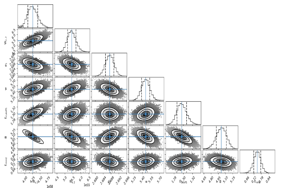
Figure 4: The corner image of knot D1+D2H3 of 3C 273.

We divide these sources into three sub-groups based on their wavelength coverage in the data-set. (1) The knots in 3C 273, shown in Figure LABEL:fig:1, have multi-wavelength measurements with the largest data-set, which provide the tightest constraint on the model parameters. We take the corner plot of knot D1+D2H3 for 3C 273 as an example to show the relationship between the different parameters in Figure 4, the maximum likelihood parameter vector is indicated with the cross. (2) The knots in the sources 3C 403, 3C 17, Pictor A, 3C 111, and PKS 2152-699 have also multi-wavelength measurements but with less data points, as shown in Figure LABEL:fig:2. For example, there is only one radio data point for the knots of 3C 403, Pictor A, and 3C 111, and the error bars in the X-ray data are slightly larger due to the lower photon statistics. (3) For the knots in 3C 353 and S5 2007+777 in Figure LABEL:fig:3, optical measurements are missing or only upper limits available. Thus the constraint on $E_{\rm cutoff1}$ and $E_{\rm min2}$ is weak.

From Table 3, we find that the parameters change only slightly for different knots in the same jet, especially for 3C 273, which contains plenty of data points. In general, the lower-energy electron population has a higher total energy content in all the sources, with $W_{\rm e,1}\sim(10^{54}-5\times 10^{58})$ ergs, while $W_{\rm e,2}\sim(10^{51}-2\times 10^{56})$ ergs for the high-energy electron population.

The magnetic field strength is in the range $B\sim(1-14)\leavevmode\nobreak\ \mu$G for the different knots. Within the jet, the magnetic field varies slightly for the different knots. For 3C 273 and 3C 403, there is a slightly increasing trend for the magnetic field strength of the knots. For the low-energy electron population, the spectral indices range from $\alpha_{\rm 1}\sim 1.8-3.2$, with a significant clustering around $2.5$, and the typical cutoff energies are in the range $E_{\rm cutoff1}\sim(0.4-26)$ TeV.

For the high-energy population, we find $E_{\rm min2}\sim(0.4-55)$ TeV and $w\sim(2-10)$. The difference in the shear viscous parameter ($w$) relates to their jet profiles through Eqs. 5 and 6. The corresponding spectral index $\alpha_{-}$ of the high-energy electron population can be obtained from Eq. 3, and is in the range $\sim 1.4-3.2$, with some significant clustering around $2$. Generally, a harder spectrum requires a higher spine velocity, as shown in Table 4. For both power-law and linearly decreasing velocity profiles we find jet-spine velocities that are mostly compatible with mildly relativistic (i.e., $\Gamma\lesssim 4$) flow speeds, perhaps apart from 3C 111 (K14), 3C 353 (W47), and 3C 17 (S11.3). In general, the derived spine velocities for a power-law profile are slightly smaller than the ones for a linear profile. There are velocity constraints or measurements for some jets (such as 3C 273 and 3C 111) from their proper motions (Meyer et al., 2016; Oh et al., 2015), our derived jet velocities are generally in agreement with them.

For different knots in the same jets, the variation of velocities ($\beta_{\rm 0,l}$ or $\beta_{\rm 0,p}$) is insignificant, suggesting that the X-ray jet can maintain its speed over a large scale. In particular, for 3C 273, the knot speeds differ only slightly. This is consistent with radio observations, which suggested that the jet of 3C 273 does not decelerate substantially from knot A to knot D1 (Meyer & Georganopoulos, 2014; Conway et al., 1993). For 3C 353, the model indicates that the jet speed is higher in knot W47 than in knot E23 and knot E88. We note that knot W47 belongs to the counter-jet (at a distance in between the other two knots), while E23 and E88 belong to the main jet (Kataoka et al., 2008).

The cut-off energy of the high-energy population can be derived from Eq. 7, and can well exceed 100 TeV (e.g., in 3C 273). In several cases, however, particularly for sources of sub-group (3), e.g., 3C 353, the cut-off energy is not really constrained given the current data. A decreasing trends of $E_{\rm e,max}$ from inner to outer knots can be found in most knots of 3C 273 and 3C 403.

In Table 4, we also show the ratio between the knot power $P_{\rm knot}$ and the Eddington luminosity $L_{\rm edd}$ for the X-ray knots in FR II jets, where we calculate $P_{\rm knot}$ based on the velocity from the linear profile,

$$P_{\rm knot}\simeq\frac{(W_{\rm e,1}+W_{\rm e,2})c\beta_{\rm 0,l}}{2L_{\rm knot}/\sin\theta},$$ (9)

where $c$ is the speed of light. As we set $E_{\rm min1}\geq 2.5\,{\rm GeV}>m_{p}c^{2}$, this is a good approximation of the jet kinetic energy. Values of the viewing angle $\theta$ for different jets are discussed in Section 2. For 3C 273, we use $\theta=7\hbox{${}^{\circ}$}$. For 3C 353 and 3C 403, we use the lower limits on the viewing angles $\theta=60\hbox{${}^{\circ}$}$ and $\theta=45\hbox{${}^{\circ}$}$, respectively. For the other sources, we adopt the upper limits of the viewing angle $\theta$. The length of the knots $L_{\rm knot}$ is listed in Table 6. Typically, the resultant knot power for the different jets is in the range $P_{\rm knot}\sim 10^{42}-10^{46}\rm erg\ s^{-1}$. For 3C 17, $\theta$ is unknown, hence the Doppler factor $\delta$ is uncertain, thus we assume $\delta=\Gamma$ to obtain $P_{\rm knot}$ for S11.3 and S3.7. In general, the required high power is essentially driven by the first electron component.

The Eddington luminosity $L_{\rm edd}=1.25\times 10^{38}\,(\rm M_{\rm BH}/\mbox{$\rm M_{\odot}$})\,\rm erg\ s^{-1}$ can be obtained using the SMBH masses ($\rm M_{\rm BH}$) reported in Section 2. We do not employ $L_{\rm edd}$ for 3C 353 and PKS 2152-699 given the lack of information on their SMBH mass. Instead, for PKS 2152-699, Breiding et al. (2023) have estimated a time-averaged jet kinetic power ($L_{\rm kin}$) $\sim 4\times 10^{44}\rm erg\ s^{-1}$, our result ($\sim 1.7\times 10^{44}\rm erg\ s^{-1}$) is consistent with their findings, which also take into account the thermal energy of the gas. For all the knots, we find that the power required to reproduce the multi-wavelength emission is smaller than the Eddington luminosity, see Table 4, i.e. $P_{\rm knot}/L_{\rm edd}\sim(10^{-4}-0.2)$.

We note that we originally did not consider beaming effects ($\delta$ = 1), except for 3C 17. However, the possibility of high flow speeds up to 0.99 (bulk Lorentz factors $\Gamma\sim$ 10) as inferred for knots HST-32 (Pictor A), K14 (3C 111), and W47 (3C 353), indicates that relativistic effects and Doppler boosting could be important, thus we obtain the Doppler factor for these knots, where $\delta^{-1}=\Gamma(1-\beta_{\rm 0,l}\cos{\theta})$ and $\Gamma=(1-\beta_{\rm 0,l}^{2})^{-\frac{1}{2}}$.

5 Summary and discussion

In this work we have studied a large sample of X-ray knots from FR II jets within the framework of gradual shear acceleration and constrained the jet properties by modeling their multi-wavelength data. For this, we reanalyzed Chandra ACIS data for 15 knots in five sources taking new observations into account, and analyzed Fermi-LAT Pass 8 data for five jets with archival data. The X-ray spectra are compatible with a single power-law model in the energy range 0.3 -7.0 keV. The resultant X-ray photon indices reveal variations ranging from 0.5 to 1.2. The photon indices in the X-ray energy band are clearly different from those in the radio and the optical band, indicating that the emission cannot be explained by synchrotron radiation from a single population of electrons. Hence we explore a scenario where two populations of electrons contribute to the observed emission. In particular, we consider the high-energy electron population to be energized by shear acceleration and being responsible for the X-rays (e.g., Tavecchio, 2021; Wang et al., 2021).

Our model for the two electron populations has seven major free parameters: the total energy ($W_{\rm e,1}$), the spectral index ($\alpha_{\rm 1}$), and the cutoff energy ($E_{\rm cutoff1}$) of the low-energy electron population, the total energy ($W_{\rm e,2}$) and the minimum energy ($E_{\rm min2}$) of the high-energy electron population, shear viscosity parameter ($w$), and the mean magnetic field ($B$), as defined in Eqs. (1-6). We use the Naima software package to perform the fitting of the multi-wavelength SEDs and to derive the best-fit and uncertainty distributions of those parameters through the MCMC algorithm. According to the wavelength coverage in the data-set, we have divided our sample into three subgroups, i.e., (1) the knots in 3C 273, (2) the knots in the sources 3C 403, 3C 17, Pictor A, 3C 111, and PKS 2159-699, (3) the knots in 3C 353 and S5 2007+777.

The results are summarized in Tables 3 and 4, and Figures LABEL:fig:1-LABEL:fig:3. We find that in these sources, the magnetic field is between $B\sim(1-14)\leavevmode\nobreak\ \mu$G. For the shear-accelerated electron population, an injection at $E_{\rm min2}\sim(0.4-55)$ TeV is required and the cutoff energy is typically around some hundreds of TeV. The shear viscous parameter ($w$) is typically in the range of $w\sim(2,10)$, corresponding to electron spectral indices $\alpha_{-}$ in the range $\sim 1.8-3.2$. With the exemption of S11.3 (3C 17) where a hard spectrum appears and where an IC/CMB interpretation might be possible due to its uncertain jet inclination, our results indicate that shear acceleration can be an efficient mechanism for accelerating electrons to high energy, producing the required particle spectra. The corresponding spine velocities are in the range $\beta_{\rm 0,l}\sim 0.69-0.99$ for a linear profile, and $\beta_{\rm 0,p}\sim 0.61-0.97$ for a power-law profile, and (with possible exception of K14, W47, and S11.3) in principle all compatible with mildly relativistic ($\Gamma\lesssim 4$), large-scale jet flow speeds. The small difference between the derived $\beta_{\rm 0,l}$ and $\beta_{\rm 0,p}$ is in agreement with the expectation that the spectral indices depend less on velocity profiles for higher-velocity spines (Rieger & Duffy, 2022; Wang et al., 2023). Within the jet, the derived velocities for different knots are statistically consistent with each other. For all the knots, we find that the required power to produce the multi-wavelength emission is smaller than the Eddington luminosity with a ratio $P_{\rm knot}/L_{\rm edd}\sim(10^{-4}-0.2)$.

The parameters of the knots in 3C 273 can be tightly constrained, which allows the study of possible variations in the knots. No significant variations are found for the parameters of the low-energy population ($E_{\rm cutoff1}$ and $\alpha_{\rm 1}$), while some variations are found for the parameters ($E_{\rm e,max}$) of the high-energy population, especially in C2 and D1+D2H3. These differences further support that the two electron populations are produced by different processes. We also found that except for C2, there is a decreasing tendency for $\alpha_{\rm X}$ and a decreasing trend for $E_{\rm e,max}$ from the inner to the outer knots, while the derived velocities are compatible with each other. The change of the magnetic field may be related to the dynamics of the jet, which can affect shear acceleration via the changing of velocity profiles or the particle injection process. This needs to be explored in the future.

The jets of AGNs are potential ultra-high-energy cosmic-ray (UHECR) accelerators according to the Hillas criterion (Hillas, 1984; Aharonian, 2002). In the framework of shear acceleration, it is found that the maximum energies UHECRs may reach is $E_{\rm p,max}\simeq 3Z\xi^{\frac{1}{2-q}}\Delta W_{\rm sh,0.1}\left(\frac{B}{30\mu\rm G}\right)\rm EeV$ (Rieger & Duffy, 2019), where $\xi\leq 1$ is the turbulence energy density ratio and $Z$ is the atomic number. Hence, in the case of strong turbulence with $\xi=1$, protons and nuclei could in principle be accelerated to $E_{\rm p,max}\sim(1-30)Z$ EeV in those FR II sources through shear acceleration. This provides further support that the large-scale jets of FR II radio galaxies could serve as UHECR accelerators.

The current analysis substantiates a picture where the X-ray emission from large-scale AGN jets is predominantly related to synchrotron radiation of a second population of electrons reaching multi-TeV energies. Meanwhile, deep multi-wavelength observations of FR II jets have revealed a general trend that the X-ray emission region is narrower than the radio one (e.g. Marchenko et al. (2017)) and displays an offset with the radio along the jet (e.g. Kataoka et al. (2008)). In the framework of shear acceleration, this may be related to the shearing profile of the jet, where the velocity gradient may be nonuniform in the jet. For example, in the outer sheath the velocity gradient can be smaller than at the interface of the spine and sheath as indicated by the simulations (Wang et al., 2023), thus the particle acceleration in the outer sheath may be less efficient. Such details can be investigated by high-resolution simulations of full jet propagation in the future.

6 data availability

The Fermi-LAT data used in this work are publicly available, which is provided online by the NASA-GSFC Fermi Science Support Center. The Chandra ACIS data used in work are publicly available, which is provided online by the Chandra Data Archive.

Appendix A Figures

Appendix B Tables

Table 5: $Chandra$ observations of the re-analyzed FR II sources.

Source	${\rm ObsID}$	${\rm ExpTime}$[ks]	${\rm StartDate}$ (YYY-MM-DD)	Source	${\rm ObsID}$	${\rm ExpTime}$[ks]	${\rm StartDate}$ (YYY-MM-DD)
3C 111	$14990$	$92.100$	$2013-01-10$	3C 273	$459$	$38.670$	$2000-01-10$
	$16219$	$143.41$	$2014-11-04$		$1711$	$27.120$	$2000-06-14$
	$19615$	$22.540$	$2017-12-26$		$1712$	$27.450$	$2000-06-14$
	$19616$	$23.500$	$2019-01-03$		$2463$	$26.690$	$2001-06-13$
	$20907$	$28.160$	$2017-12-29$		$2464$	$29.460$	$2001-06-13$
	$20908$	$27.230$	$2017-12-29$		$2471$	$24.890$	$2001-06-15$
	$22023$	$15.690$	$2018-12-30$		$3456$	$24.530$	$2002-06-05$
	$22024$	$19.600$	$2018-12-29$		$3457$	$24.850$	$2002-06-05$
	$22025$	$16.180$	$2019-01-06$		$3574$	$29.340$	$2002-06-04$
	$22026$	$12.760$	$2019-01-07$		$4430$	$27.150$	$2003-07-07$
3C 403	$2968$	$49.470$	$2002-12-07$		$4431$	$26.420$	$2003-07-07$
	$12741$	$7.9500$	$2010-11-27$		$4876$	$37.460$	$2003-11-24$
PKS 2152-699	$11530$	$56.750$	$2010-01-22$		$4877$	$34.860$	$2004-02-10$
	$12088$	$58.360$	$2010-01-20$		$4878$	$34.090$	$2004-04-26$
	$16083$	$121.17$	$2014-07-19$		$4879$	$35.580$	$2004-07-28$
	$16084$	$57.310$	$2014-07-16$		$5169$	$29.680$	$2004-06-30$
S5 2007+777	$5709$	$36.050$	$2005-05-23$		$5170$	$28.400$	$2004-06-30$
					$7364$	$2.0100$	$2007-01-15$
					$7365$	$2.1200$	$2007-07-10$
					$8375$	$29.550$	$2007-06-25$
					$9703$	$29.700$	$2008-05-08$
					$14455$	$29.550$	$2012-07-16$
					$17393$	$29.540$	$2015-07-14$
					$18421$	$29.600$	$2016-06-27$
					$19867$	$26.910$	$2017-06-26$
					$20709$	$29.570$	$2018-07-04$
					$21815$	$29.590$	$2019-07-03$
					$22828$	$28.410$	$2020-07-06$
					$24585$	$25.590$	$2021-06-10$

Table 6: X-ray positions and sizes of the knots

Source	Knot	${\rm RA(hh:mm:ss)}$	${\rm Dec(dd:mm:ss)}$	${L_{\rm knot}(\rm\arcsec)}$b	${W_{\rm knot}(\rm\arcsec)}$c
3C 273 a	A	$12:29:06.14$	$+02:02:58.87$	0.94 (2.53 $\rm kpc)$	1.33 (3.60 $\rm kpc)$
	B1+B2	$12:29:06.03$	$+02:02:57.55$	0.94 (2.53 $\rm kpc)$	1.31 (3.53 $\rm kpc)$
	B3+C1	$12:29:05.94$	$+02:02:56.13$	0.77 (2.08 $\rm kpc)$	1.05 (2.84 $\rm kpc)$
	C2	$12:29:05.88$	$+02:02:55.11$	0.70 (1.89 $\rm kpc)$	1.02 (2.76 $\rm kpc)$
	D1+D2H3	$12:29:05.81$	$+02:02:53.62$	1.01 (2.72 $\rm kpc)$	1.02 (2.74 $\rm kpc)$
3C 403	F1	$19:52:19.12$	$+02:30:33.30$	3.60 (4.06 $\rm kpc)$	3.60 (4.06 $\rm kpc)$
	F6	$19:52:17.57$	$+02:30:33.20$	3.60 (4.06 $\rm kpc)$	3.60 (4.06 $\rm kpc)$
3C 17	S3.7	$00:38:20.77$	$-02:07:41.60$	0.46 (1.60 $\rm kpc)$	0.18 (0.60 $\rm kpc)$
	S11.3	$00:38:21.20$	$-02:07:45.90$	0.40 (1.40 $\rm kpc)$	0.30 (1.00 $\rm kpc)$
Pictor A	HST-32	$05:19:46.69$	$-45:46:37.35$	3.60 (2.48 $\rm kpc)$	3.60 (2.48 $\rm kpc)$
	HST-106	$05:19:39.73$	$-45:46:22.80$	3.60 (2.48 $\rm kpc)$	3.60 (2.48 $\rm kpc)$
	HST-112	$05:19:39.20$	$-45:46:21.80$	4.00 (2.80 $\rm kpc)$	2.00 (1.40 $\rm kpc)$
3C 111	K14	$04:18:22.50$	$+38:01:43.06$	3.60 (3.42 $\rm kpc$)	3.60 (3.42 $\rm kpc$)
	K30	$04:18:23.48$	$+38:01:50.60$	2.49 (2.42 $\rm kpc)$	1.55 (1.50 $\rm kpc)$
	K61	$04:18:25.66$	$+38:02:05.26$	2.89 (2.80 $\rm kpc)$	2.13 (2.07 $\rm kpc)$
PKS 2152-699	D	$21:57:07.07$	$-69:41:14.77$	1.73 (0.97 $\rm kpc)$	1.73 (0.97 $\rm kpc)$
3C 353	E23	$17:20:29.70$	$-00:58:41.60$	1.20 (0.72 $\rm kpc$)	1.20 (0.72 $\rm kpc$)
	E88	$17:20:32.80$	$-00:58:26.60$	1.50 (0.90 $\rm kpc$)	1.50 (0.90 $\rm kpc$)
	W47	$17:20:29.70$	$-00:58:41.60$	2.00 (1.20 $\rm kpc$)	2.00 (1.20 $\rm kpc$)
S5 2007+777	K3.6	$20:05:30.25$	$+77:52:42.31$	0.83 (3.98 $\rm kpc)$	0.83 (3.98 $\rm kpc)$
	K5.2	$20:05:29.69$	$+77:52:42.50$	0.62 (3.00 $\rm kpc)$	0.62 (3.00 $\rm kpc)$
	K8.5	$20:05:28.45$	$+77:52:41.18$	0.62 (3.00 $\rm kpc)$	0.62 (3.00 $\rm kpc)$
	K11.1	$20:05:27.51$	$+77:52:39.39$	0.62 (3.00 $\rm kpc)$	0.62 (3.00 $\rm kpc)$
	K15.9	$20:05:26.29$	$+77:52:38.66$	0.62 (3.00 $\rm kpc)$	0.62 (3.00 $\rm kpc)$

• As the adjacent knots in 3C 273 jet cannot be resolved in the X-ray band, we combined multiple knot regions to perform the spectral analysis.

• $L_{\rm knot}$ is the half width at half maximum along the jet.

• $W_{\rm knot}$ is the half width at half maximum transverse to the jet. The $L_{\rm knot}$ and $W_{\rm knot}$ of 3C 273, 3C 17, 3C 353, and Pictor A are taken from Jester et al. (2006), Massaro et al. (2009), Kataoka et al. (2008), and Gentry et al. (2015), respectively.

References

- Abdo et al. (2010) Abdo A. A., et al., 2010, Science, 328, 725
- Abramowitz & Stegun (1972) Abramowitz M., Stegun I. A., 1972, Handbook of Mathematical Functions
- Aharonian (2002) Aharonian F. A., 2002, MNRAS, 332, 215
- Atwood et al. (2009) Atwood W. B., et al., 2009, ApJ, 697, 1071
- Ballet et al. (2020) Ballet J., Burnett T. H., Digel S. W., Lott B., 2020, arXiv e-prints, p. arXiv:2005.11208
- Barthel (1989) Barthel P. D., 1989, ApJ, 336, 606
- Boccardi et al. (2016) Boccardi B., Krichbaum T. P., Bach U., Mertens F., Ros E., Alef W., Zensus J. A., 2016, A&A, 585, A33
- Breiding et al. (2023) Breiding P., Meyer E. T., Georganopoulos M., Reddy K., Kollmann K. E., Roychowdhury A., 2023, MNRAS, 518, 3222
- Cara et al. (2013) Cara M., et al., 2013, ApJ, 773, 186
- Celotti et al. (2001) Celotti A., Ghisellini G., Chiaberge M., 2001, MNRAS, 321, L1
- Clautice et al. (2016) Clautice D., et al., 2016, ApJ, 826, 109
- Conway et al. (1993) Conway R. G., Garrington S. T., Perley R. A., Biretta J. A., 1993, A&A, 267, 347
- Domínguez et al. (2011) Domínguez A., et al., 2011, MNRAS, 410, 2556
- Fanaroff & Riley (1974) Fanaroff B. L., Riley J. M., 1974, MNRAS, 167, 31P
- Foreman-Mackey et al. (2013) Foreman-Mackey D., Hogg D. W., Lang D., Goodman J., 2013, PASP, 125, 306
- Fosbury et al. (1998) Fosbury R. A. E., Morganti R., Wilson W., Ekers R. D., di Serego Alighieri S., Tadhunter C. N., 1998, MNRAS, 296, 701
- Gentry et al. (2015) Gentry E. S., et al., 2015, ApJ, 808, 92
- Georganopoulos & Kazanas (2003) Georganopoulos M., Kazanas D., 2003, ApJ, 589, L5
- Georganopoulos et al. (2016) Georganopoulos M., Meyer E., Perlman E., 2016, Galaxies, 4, 65
- Guo et al. (2018) Guo S.-C., Zhang H.-M., Zhang J., Liang E.-W., 2018, Research in Astronomy and Astrophysics, 18, 070
- H. E. S. S. Collaboration et al. (2020) H. E. S. S. Collaboration et al., 2020, Nature, 582, 356
- Hardcastle et al. (2001) Hardcastle M. J., Birkinshaw M., Worrall D. M., 2001, MNRAS, 326, 1499
- Hardcastle et al. (2016) Hardcastle M. J., et al., 2016, MNRAS, 455, 3526
- Harris & Krawczynski (2006) Harris D. E., Krawczynski H., 2006, ARA&A, 44, 463
- Hillas (1984) Hillas A. M., 1984, ARA&A, 22, 425
- Ito et al. (2021) Ito S., Inoue Y., Kataoka J., 2021, ApJ, 916, 95
- Jester et al. (2005) Jester S., Röser H. J., Meisenheimer K., Perley R., 2005, A&A, 431, 477
- Jester et al. (2006) Jester S., Harris D. E., Marshall H. L., Meisenheimer K., 2006, ApJ, 648, 900
- Jester et al. (2007) Jester S., Meisenheimer K., Martel A. R., Perlman E. S., Sparks W. B., 2007, MNRAS, 380, 828
- Kataoka et al. (2008) Kataoka J., et al., 2008, ApJ, 685, 839
- Kraft et al. (2002) Kraft R. P., Forman W. R., Jones C., Murray S. S., Hardcastle M. J., Worrall D. M., 2002, ApJ, 569, 54
- Kraft et al. (2005) Kraft R. P., Hardcastle M. J., Worrall D. M., Murray S. S., 2005, ApJ, 622, 149
- Kundu & Gupta (2014) Kundu E., Gupta N., 2014, MNRAS, 444, L16
- Lemoine (2019) Lemoine M., 2019, Phys. Rev. D, 99, 083006
- Liu et al. (2017) Liu R.-Y., Rieger F. M., Aharonian F. A., 2017, ApJ, 842, 39
- Ly et al. (2005) Ly C., De Young D. S., Bechtold J., 2005, ApJ, 618, 609
- Marchenko et al. (2017) Marchenko V., Harris D. E., Ostrowski M., Stawarz Ł., Bohdan A., Jamrozy M., Hnatyk B., 2017, ApJ, 844, 11
- Massaro et al. (2009) Massaro F., Harris D. E., Chiaberge M., Grandi P., Macchetto F. D., Baum S. A., O’Dea C. P., Capetti A., 2009, ApJ, 696, 980
- McKeough et al. (2016) McKeough K., et al., 2016, ApJ, 833, 123
- Meyer & Georganopoulos (2014) Meyer E. T., Georganopoulos M., 2014, ApJ, 780, L27
- Meyer et al. (2016) Meyer E. T., et al., 2016, ApJ, 818, 195
- Mondal & Gupta (2019) Mondal S., Gupta N., 2019, Astroparticle Physics, 107, 15
- Nagai et al. (2014) Nagai H., et al., 2014, ApJ, 785, 53
- Oh et al. (2015) Oh J., et al., 2015, Journal of Korean Astronomical Society, 48, 299
- Paltani & Türler (2005) Paltani S., Türler M., 2005, A&A, 435, 811
- Perlman et al. (2001) Perlman E. S., Biretta J. A., Sparks W. B., Macchetto F. D., Leahy J. P., 2001, ApJ, 551, 206
- Perlman et al. (2020) Perlman E. S., Clautice D., Avachat S., Cara M., Sparks W. B., Georganopoulos M., Meyer E., 2020, Galaxies, 8, 71
- Rahman et al. (2023) Rahman A. A., Sahayanathan S., Zahoor M., Subha P. A., 2023, arXiv e-prints, p. arXiv:2302.08111
- Rieger (2019) Rieger F. M., 2019, Galaxies, 7, 78
- Rieger & Duffy (2004) Rieger F. M., Duffy P., 2004, ApJ, 617, 155
- Rieger & Duffy (2019) Rieger F. M., Duffy P., 2019, ApJ, 886, L26
- Rieger & Duffy (2021) Rieger F. M., Duffy P., 2021, ApJ, 907, L2
- Rieger & Duffy (2022) Rieger F. M., Duffy P., 2022, ApJ, 933, 149
- Rieger et al. (2007) Rieger F. M., Bosch-Ramon V., Duffy P., 2007, Ap&SS, 309, 119
- Sambruna et al. (2001) Sambruna R. M., Urry C. M., Tavecchio F., Maraschi L., Scarpa R., Chartas G., Muxlow T., 2001, ApJ, 549, L161
- Sambruna et al. (2008a) Sambruna R. M., Donato D., Cheung C. C. Tavecchio F., Maraschi L., 2008a, in Rector T. A., De Young D. S., eds, Astronomical Society of the Pacific Conference Series Vol. 386, Extragalactic Jets: Theory and Observation from Radio to Gamma Ray. p. 94 (arXiv:0707.1321)
- Sambruna et al. (2008b) Sambruna R. M., Donato D., Cheung C. C., Tavecchio F., Maraschi L., 2008b, ApJ, 684, 862
- Sikora et al. (2007) Sikora M., Stawarz Ł., Lasota J.-P., 2007, ApJ, 658, 815
- Sun et al. (2018) Sun X.-N., Yang R.-Z., Rieger F. M., Liu R.-Y., Aharonian F., 2018, A&A, 612, A106
- Swain et al. (1998) Swain M. R., Bridle A. H., Baum S. A., 1998, ApJ, 507, L29
- Tavecchio (2021) Tavecchio F., 2021, MNRAS, 501, 6199
- Tavecchio et al. (2000) Tavecchio F., Maraschi L., Sambruna R. M., Urry C. M., 2000, ApJ, 544, L23
- Tingay et al. (2000) Tingay S. J., et al., 2000, AJ, 119, 1695
- Uchiyama et al. (2006) Uchiyama Y., et al., 2006, ApJ, 648, 910
- Vasudevan et al. (2010) Vasudevan R. V., Fabian A. C., Gandhi P., Winter L. M., Mushotzky R. F., 2010, MNRAS, 402, 1081
- Wang et al. (2020) Wang Z.-J., Zhang J., Sun X.-N., Liang E.-W., 2020, ApJ, 893, 41
- Wang et al. (2021) Wang J.-S., Reville B., Liu R.-Y., Rieger F. M., Aharonian F. A., 2021, MNRAS, 505, 1334
- Wang et al. (2023) Wang J.-S., Reville B., Mizuno Y., Rieger F. M., Aharonian F. A., 2023, MNRAS, 519, 1872
- Webb et al. (2018) Webb G. M., Barghouty A. F., Hu Q., le Roux J. A., 2018, ApJ, 855, 31
- Webb et al. (2019) Webb G. M., Al-Nussirat S., Mostafavi P., Barghouty A. F., Li G., le Roux J. A., Zank G. P., 2019, ApJ, 881, 123
- Webb et al. (2020) Webb G. M., Mostafavi P., Al-Nussirat S., Barghouty A. F., Li G., le Roux J. A., Zank G. P., 2020, ApJ, 894, 95
- Weisskopf et al. (2002) Weisskopf M. C., Brinkman B., Canizares C., Garmire G., Murray S., Van Speybroeck L. P., 2002, PASP, 114, 1
- Werner et al. (2012) Werner M. W., Murphy D. W., Livingston J. H., Gorjian V., Jones D. L., Meier D. L., Lawrence C. R., 2012, ApJ, 759, 86
- Worrall et al. (2012) Worrall D. M., Birkinshaw M., Young A. J., Momtahan K., Fosbury R. A. E., Morganti R., Tadhunter C. N., Verdoes Kleijn G., 2012, MNRAS, 424, 1346
- Wu et al. (2002) Wu X.-B., Liu F. K., Zhang T. Z., 2002, A&A, 389, 742
- Wu et al. (2017) Wu J., Ghisellini G., Hodges-Kluck E., Gallo E., Ciardi B., Haardt F., Sbarrato T., Tavecchio F., 2017, MNRAS, 468, 109
- Zabalza (2015) Zabalza V., 2015, in 34th International Cosmic Ray Conference (ICRC2015). p. 922 (arXiv:1509.03319)
- Zhang et al. (2009) Zhang W., MacFadyen A., Wang P., 2009, ApJ, 692, L40
- Zhang et al. (2010) Zhang J., Bai J. M., Chen L., Liang E., 2010, ApJ, 710, 1017
- Zhang et al. (2018a) Zhang J., Du S.-s., Guo S.-C., Zhang H.-M., Chen L., Liang E.-W., Zhang S.-N., 2018a, ApJ, 858, 27
- Zhang et al. (2018b) Zhang J., Zhang H.-M., Yao S., Guo S.-C., Lu R.-J., Liang E.-W., 2018b, ApJ, 865, 100
- Zirakashvili & Aharonian (2007) Zirakashvili V. N., Aharonian F., 2007, A&A, 465, 695