Towards Clip-Free Quantized Super-Resolution Networks: How to Tame Representative Images

Abstract

Super-resolution (SR) networks have been investigated for a while, with their mobile and lightweight versions gaining noticeable popularity recently. Quantization, the procedure of decreasing the precision of network parameters (mostly FP32 to INT8), is also utilized in SR networks for establishing mobile compatibility. This study focuses on a very important but mostly overlooked post-training quantization (PTQ) step: representative dataset (RD), which adjusts the quantization range for PTQ. We propose a novel pipeline (clip-free quantization pipeline, CFQP) backed up with extensive experimental justifications to cleverly augment RD images by only using outputs of the FP32 model. Using the proposed pipeline for RD, we can successfully eliminate unwanted clipped activation layers, which nearly all mobile SR methods utilize to make the model more robust to PTQ in return for a large overhead in runtime. Removing clipped activations with our method significantly benefits overall increased stability, decreased inference runtime up to 54% on some SR models, better visual quality results compared to INT8 clipped models - and outperforms even some FP32 non-quantized models, both in runtime and visual quality, without the need for retraining with clipped activation.

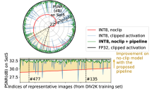
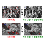
Figure 1: PSNR on Set5 [Bevilacqua et al.(2012)Bevilacqua, Roumy, Guillemot, and line Alberi Morel] for XCAT [Ayazoglu and Bilecen(2023)] (radial & y-axis), where the model is individually quantized with 800 different representative images on DIV2K [Agustsson and Timofte(2017)] (angular & x-axis). We aim to get closer to the circumference. For clarity, we sort INT8 no-clip PSNR values (red) and use the same sorted indices for the rest. The no-clip INT8 XCAT model with CFQP outperforms the same model when RD is not augmented.The no-clip INT8 model with CFQP yields fewer outliers in the output data (right), increasing the visual quality.

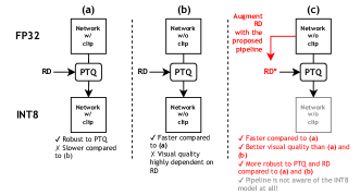
Figure 2: Most SR networks to be gone under PTQ includes a clipped activation at the end to limit the output range (a). If the clip is removed, the visual quality gets very unstable (i.e., not robust to PTQ) (b), most of the time making the network useless. We propose an RD augmentation pipeline (CFQP, c), which only utilizes the outputs of the FP32 model to be quantized and show significant improvements over (a) & (b).

1 Introduction

Super-resolution (SR) is a widely studied ill-posed inverse problem that involves generating high-resolution (HR) images from low-resolution (LR) ones. Despite remarkable progress achieved through deep learning on SR networks, the emphasis has been predominantly on enhancing the quality of SR results rather than addressing the efficiency and deployment challenges associated with resource-constrained mobile platforms. One promising technique to address this challenge is post-training quantization (PTQ), which compresses the model size by decreasing the precision of network parameters (commonly from FP32 to INT8), reducing the inference time.

However, despite its effectiveness, PTQ can significantly drop network performance if not applied correctly. It becomes more critical, especially on low-level computer vision tasks such as SR. Recent advancements in efficient & mobile SR methods [Ayazoglu(2021), Ignatov et al.(2021)Ignatov, Timofte, Denna, and Younes, Ignatov and Timofte(2023), Li et al.(2022)Li, Zhang, Timofte, and Gool, Zamfir et al.(2023)Zamfir, Conde, and Timofte, Conde et al.(2023)Conde, Zamfir, Timofte, et al.] reveal that using a clipped activation layer (mostly clipped ReLU) at the end of the network model aids in keeping the visual quality consistent in FP32 training and PTQ processes, but with a cost of an increase in the inference which is more noticeable on limited hardware. The clipping operation helps PTQ to be more stable because the FP32 model has already been forced to map its output values to the correct range. Hence, quantizing those values would not yield out-of-range results, keeping the output visual quality consistent between INT8 and FP32 models as much as possible.

That said, one very important yet neglected part of these previously followed procedures is that PTQ already determines a range for the quantization internally (hence the clipping range) using the given representative dataset (RD). This means that most of the previous studies have not selected their representative datasets with any optimization, hence having to rely on the additional clipped activation at the network’s end to force the PTQ to set its quantization range to whatever the clipped activation layer’s range is. Most other works use all the training set, take random subsets, or individual images to construct RD. Still, they do not have an optimized approach and do not aim to eliminate the clipped activations for SR models.

Hence, this paper aims to optimize the overlooked part of choosing RD by performing extensive experiments and observations. Based on our observations, we propose clip-free quantization pipeline (CFQP) for RD to make the INT8 network more robust to PTQ, which eliminates the need for clipped activations to keep the visual quality consistent (Figure 1 and 2.c). Our pipeline consists of determining good and bad images for PTQ based on the number of outlier pixel numbers and ranges, and improves the bad ones only by utilizing the outputs of the corresponding FP32 model. Our contributions are as follows:

• We prove that the RD’s for SR yields better performance when they only have a single representative image (RI), eliminating the need for constructing an unnecessarily large RD. This also serves as one-shot quantization.

• We show that even if the model is trained with RGB images, choosing RD as grayscale yields much higher PSNR scores after PTQ compared to RGB.

• We determine whether an image is a good or a bad RI candidate by only looking at the output response of corresponding FP32 models.

• We propose CFQP to augment and improve bad RI’s, which improve the overall INT8 model and eliminate the need for clipped activations. The no-clip INT8 models with our modified RI’s outperform the same no-clip and clipped INT8 models without augmented RI’s, and even some FP32 models in terms of PSNR. With a high ratio (99.1%), our proposed pipeline makes every bad image a good candidate for RI.

• Given the need for clipped activations is alleviated, we achieve significant SR model inference speedups (up to 54%) compared to their clipped counterparts on various mobile devices.

2 Related Work

Quantization is frequently used and applied on image/video SR models, motivated by the ongoing challenges and related workshops [Ignatov and Timofte(2023), Li et al.(2022)Li, Zhang, Timofte, and Gool]. In addition, there are also studies to improve quantization accuracy, like using new quantization-aware loss functions [Zhuo et al.(2022)Zhuo, Chen, Ramakrishnan, Chen, Feng, Lin, Zhang, and Shen] or rearranging activation functions like clipping [Choi et al.(2018)Choi, Wang, Venkataramani, Chuang, Srinivasan, and Gopalakrishnan]. On the other hand, there are some notable works on representative dataset (RD) effects. PTQ and RD are considered together in cross-domain calibration studies [Haichao Yu(2021)]. However, it does not aim to classify good representative images in the training dataset and improve others. Besides the cross-domain, dataset distillation is also a recent field to create a condensed dataset, but generally aimed at training networks and includes no alteration in image content [Ruonan Yu(2023)].

Apart from these, Zhang et al. proposed a method to select representative images for PTQ [Zhang et al.(2022)Zhang, Gao, Fan, Zhao, Yang, and Yan]. They use clustering: which may vary for different datasets, does not benefit from the FP32 model output information, and does not try to improve the bad-performing representative images, unlike ours. Yuan et alalso did some benchmark tests considering PTQ [Yuan et al.(2023)Yuan, Liu, Wu, Yang, Wu, Sun, Liu, Wang, and Wu]. In a small section, they mention a calibration dataset selection. Still, it does not include a detailed investigation, and we have shown some conflicting results with justifications about the selection of representative dataset size.

3 Preliminary Experiments

In this section, we explain our setup and ask & answer the relevant questions related to the selection of RD. We have conducted multiple experiments to find satisfying answers to the proposed questions, ultimately leading us to our CFQP proposal.

3.1 Model Selection and Training

We utilize 5 mobile-friendly, diverse in structure & activations SR models with upscaling rate x3: XCAT [Ayazoglu and Bilecen(2023)], ABPN [Du et al.(2021)Du, Liu, Tang, and Wu], ESPCN [Shi et al.(2016)Shi, Caballero, Huszar, Totz, Aitken, Bishop, Rueckert, and Wang], FSRCNN [Dong et al.(2016)Dong, Loy, and Tang], and RFDNNet [Liu et al.(2020)Liu, Tang, and Wu]. The selection of networks and the reason for x3 is to be consistent with the recent and comparable mobile SR challanges [Conde et al.(2023)Conde, Zamfir, Timofte, et al., Ignatov and Timofte(2023), Li et al.(2022)Li, Zhang, Timofte, and Gool]. If the clip is enabled, we trained with clipped ReLU at the end of the networks. We opted for TensorFlow (TF) for training FP32 models and applied INT8 PTQ using TensorFlow Lite. We also considered ONNX and PyTorch; however, we stuck with our decision due to TF being the most mature one in model quantization. Models are trained for 400 epochs, each consuming randomly picked 16x16 low-resolution patches from DIV2K [Agustsson and Timofte(2017)] training set (800 images) with a batch size of 8. We stick with DIV2K for quantization experiments because we noticed that mobile networks do not benefit from the abundance of training data due to their small number of parameters, although Flickr has nearly thrice of images compared to DIV2K (Table 6). We use all images of the DIV2K validation set for validation. Adam optimizer is utilized with $\beta_{1,2}$ = 0.99 and 0.999, respectively. The learning rate schedule is as follows: we start the training with 4e-4, linearly increase to 25e-4 in the first ten epochs, and decrease to 4e-5 in the remaining epochs. We employ Set5 [Bevilacqua et al.(2012)Bevilacqua, Roumy, Guillemot, and line Alberi Morel] for the test set and measure all PSNR values on the Y channels, compliant with the common convention. For quantization, static-PTQ is used. From now on, PTQ denotes static-PTQ unless specified otherwise.

3.2 Observations

Models	XCAT				ABPN				ESPCN				FSRCNN				RFDNNet
Precision	FP32		INT8		FP32		INT8		FP32		INT8		FP32		INT8		FP32		INT8
Clip	✓	✗	✓	✗	✓	✗	✓	✗	✓	✗	✓	✗	✓	✗	✓	✗	✓	✗	✓	✗
$PSNR_{R=RGB}$	32.87	32.98	32.63	26.57	33.13	33.18	32.85	26.13	32.23	32.23	31.18	24.92	32.83	32.83	31.35	25.69	33.02	32.97	32.23	25.62
$PSNR_{R=Gray}$			32.31	28.48			32.52	28.44			30.85	26.26			31.12	27.24			31.76	27.05
$\Delta_{R=RGB}$	-0.11		6.06		-0.05		6.72		$\sim$0		6.26		$\sim$0		5.66		-0.05		6.61
$\Delta_{R=Gray}$			3.83				4.08				4.59				3.88				4.71

Table 1: Average PSNR of the investigated SR models evaluated on Set5. R=RGB and R=Gray indicate the channels of the representative image for INT8 PTQ. $\Delta$ is the PSNR difference between clip and no-clip models. Note that we construct 800 different RD’s with a single image for each network, then average the resulting INT8 networks’ PSNR values.

Do clipped activations really affect PTQ? Table 1 clearly shows that removing the clip without any additional care for INT8 PTQ hinders the PSNR drastically ($\Delta$ values), but increases the latency significantly as shown in Table 5. Therefore, it is worthwhile to eliminate the clipped activation without sacrificing the visual quality since PTQ inherently applies clipping to the network by using the data statistics in RD anyway.

Hence, now the issue boils down to how to characterize RD such that it can replace the clipped activation layer.

RD Size	RD	XCAT				ABPN				ESPCN				FSRCNN				RFDNNet
		all RD	min	max	avg	all RD	min	max	avg	all RD	min	max	avg	all RD	min	max	avg	all RD	min	max	avg
5	Good images	32.84	32.57	32.85	32.72	33.11	32.86	33.11	33.00	31.44	30.86	31.82	31.53	32.03	30.41	32.01	31.40	32.28	29.79	32.16	31.54
5	Bad images	22.95	22.95	25.70	24.05	20.93	20.93	24.84	23.41	20.20	20.20	23.43	21.94	21.48	21.47	24.85	23.49	21.60	21.72	24.09	23.16
5	Random selections from good and bad	23.69	23.47	32.85	29.50	24.22	24.39	33.11	29.67	21.74	21.83	31.79	28.04	22.40	21.83	31.79	28.04	23.08	21.83	31.79	28.04
		22.95	22.95	31.71	27.22	20.93	20.93	33.04	26.87	20.20	20.20	31.82	25.46	21.47	21.47	31.80	26.60	21.71	21.72	31.89	26.11
		22.95	22.95	32.86	28.95	20.93	20.93	33.04	28.83	20.20	20.20	31.79	27.21	21.47	21.47	31.49	27.77	21.72	21.72	32.04	27.89
10	Good + bad	22.95	22.95	32.85	28.38	20.93	20.93	33.11	28.20	20.20	20.20	31.82	26.73	21.48	21.47	32.02	27.44	21.60	21.72	32.16	27.35
100	DIV2K training images	22.08	22.08	32.85	28.19	21.61	21.61	33.06	28.13	19.87	19.87	31.79	26.04	19.40	31.96	19.39	26.89	20.75	20.72	32.04	26.83

Table 2: The effect of the size of RD on Set5 PSNR for no-clip INT8 models. all RD denotes the PSNR where the model is quantized with all images in RD. We also pick each image from the RD’s stated with their sizes, create new RD’s with size one, perform PTQ, evaluate the INT8 models, and state the resulting PSNR’s min, max, and avg values. Notice that the existence of bad images inside RD considerably decreases the overall performance.

Does the number of images in RD affect the PTQ quality? In our study, good RD images are the ones that have the smallest PSNR difference between their clipped INT8 and no-clip INT8 models, and vice versa for the bad ones. We experimented with different-sized RD’s and concluded that including only a single image in the RD during PTQ is the most straightforward and tractable solution. This is because if there are multiple images in the RD, bad representative images are observed to overpower the others and lead to a worse quantized model in the end, too. This can be observed from the results in Table 2.

From now on, we continue with RD’s only consisting of a single image. RD with size one and representative image (RI) denote the same concept unless specified otherwise.

Is PTQ dependent on the number of channels of RI? Table 1 reveals that the PSNR differences between INT8 clipped and no-clip models ($\Delta$) are minimized when the RI is chosen as grayscale instead of RGB. Hence, it would be more logical to work on grayscale representative images and try to make $\Delta$ as small as possible by altering them. Note that this is surprisingly valid when the input images to the network are RGB, but the RI is grayscale.

From now on, we continue with RIs only consisting of a grayscale image.

What can indicate good representative images? To find a common point in those good images, we construct 800 grayscale RI’s, perform PTQ on five different no-clip & clipped FP32 SR models, and evaluate the resulting INT8 models on Set5. The findings are given in Figure 3.

One interesting finding is that the response of the FP32 network to the corresponding representative image yields a correlation with $\Delta_{R=Gray}$ in Table 1. To see it in action, consider image #234 in DIV2K training set in Figure 3. The corresponding models when RI is set as #234 have significant PSNR gaps between their clipped INT8 and the no-clip INT8 models (hence #234 is a bad image). Then, when #234 is given to no-clip FP32 models (XCAT is considered for demonstration without loss of generality), 26.6% of the output pixels are observed to be out-of-range (>255, <0). Note that the more out-of-range the FP32 outputs (red areas in Figure 3), the more it is inclined towards yielding a lower PSNR. The opposite happens for #235, where even some no-clip INT8 models perform better than their clipped counterparts (negative $\Delta_{R=Gray}$, a very good image for RI).

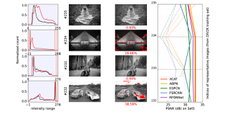
Figure 3: PSNR scores of some of the quantized SR models with different representative images (right). Dashed lines are no-clip INT8 models, and solid lines are clipped INT8. The response of corresponding FP32 models when the selected representative images are given as inputs (middle). Outlier pixels are marked with red, stated with their percentages. The histograms of the input (black) and output data (red) of the FP32 model (left), where the red areas in the histograms match with the distribution of outlier pixels.

Hence, we conclude that the number of outliers in the FP32 model’s response to the corresponding RI gives us a measure of whether the image is good or bad, correlated with $\Delta_{R=Gray}$. Therefore, if we reduce the outliers, we may also decrease $\Delta_{R=Gray}$ and increase the PTQ stability. This also means that we can understand whether a representative image would be considered as good or bad without performing PTQ. Then, if we correctly identify and use good representative images, we can omit the clipped activation layer without any loss in the INT8 model.

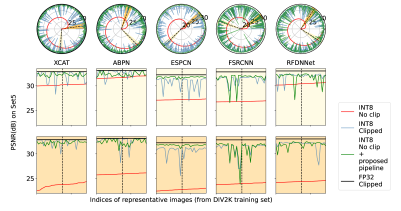
Figure 7: PSNR on Set5 (radial & y-axis) for different models, where each model is quantized with different RI selections (angular & x-axis). Our proposed pipeline applied on the no-clip INT8 (green) outperforms the no-clip INT8 by directly using RI images (red). For clarity, we sort INT8 no-clip PSNR values (red) and use the same sorted indices for the rest of the data for consistency.

Even though Figure 3 only shows a very small subset of possible RIs, we show our proposal’s positive effect and generalizability in Figure 7 later on. It is also worth noting that we also investigated other image characteristics (like their histograms) before passing it through the no-clip FP32 network but did not capture relevant correlations with the PTQ quality (Table 3, 4). We also experimented with masking out the outlier sections with other healthy regions from the same image but did not achieve satisfactory results.

Models	#105$\rightarrow$#508	#508	#105	#001$\rightarrow$#216	#216	#001	#416$\rightarrow$#176	#176	#416
XCAT	22.472	22.956	32.860	22.982	23.471	32.850	29.403	23.764	32.716
ABPN	21.980	20.933	33.026	22.445	24.849	33.115	29.418	24.195	32.864
ESPCN	23.720	20.208	31.544	24.382	21.838	31.628	28.856	21.654	31.820
FSRCNN	21.564	21.475	31.492	21.879	24.497	32.019	19.394	24.233	31.801
RFDNNet	23.955	21.723	32.044	20.463	23.454	32.165	26.044	24.098	31.893

Table 3: PSNR on Set5 for no-clip INT8 models, where histogram matching is applied to RI images. # denote the image index in DIV2K training set. When good image histograms are mapped onto the bad ones, an improvement is not observed, showing that the histogram is not a correlation factor.

	XCAT				ABPN				ESPCN				FSRCNN				RFDNNet
	0°	90°	180°	270°	0°	90°	180°	270°	0°	90°	180°	270°	0°	90°	180°	270°	0°	90°	180°	270°
#105	32.86	32.83	32.87	32.86	33.03	33.05	32.78	32.99	31.54	31.53	31.36	31.64	31.49	31.43	31.38	31.51	32.04	31.59	32.20	32.14
#508	22.96	23.25	23.21	22.64	20.93	20.61	21.24	18.79	20.21	20.07	19.29	20.02	21.48	21.52	21.62	20.89	21.72	21.63	22.07	21.90

Table 4: PSNR on Set5 for no-clip INT8 models, where given RI’s are rotated. Despite the rotation not changing the histogram, the output PNSR’s are different.

How can be systematically find good representative images and improve the bad ones? The procedure of finding good & bad images based on the previous observations is easy: if the image yields low the number of outlier pixels after the no-clip FP32 model, then quantizing that no-clip FP32 model with that image set as the representative will yield a well-performing no-clip INT8 model, and vice versa for the bad one. What about improving the bad RIs? At this stage, we propose our RI augmentation pipeline (CFQP) in Section 4.

4 Methods and Pipeline

This section presents our two methods for choosing good RI’s and improving the bad ones. Ultimately, we combine those methods to create CFQP.

Method #1: Good Representative Selection: Method #1 given in Figure 4 aims to separate good RI from bad. Based on the previous observations, we put three constraints that a good RI needs to satisfy after passing through the FP32 network: it has zero outliers, has to have min-max values close to 0-255, and its min-max values need not deviate much from the min-max of the original RI. All algorithmic design parameters are discussed in Section 3 and observed to be valid for most of the considered data. The first and second constraints stem from avoiding dividing the pixel values into 255 bins during PTQ, therefore eliminating decreasing the quantization quality due to having wider bins than required. The third constraint ensures that the FP32 model does not change or shift the pixel distribution of RI, as this will also cause the inferred images from the INT8 model to have color shifts, making the network unpractical. We empirically tuned the maximum min-max pixel difference to 5, deviation pixel difference to 5, maximum out-of-range pixels threshold as 25, and maximum shift thresholds as 10, respectively, by using 10 images from the DIV2K train set. These hyperparameters are easy to adjust, and our choices are observed to work on nearly all DIV2K train set (800 images).

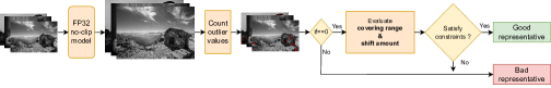
Figure 4: The procedure of selecting good representative images.

Table 7 shows the PSNR values of these selected images for different models. As seen, the images selected by Method #1 are confirmed to be the good ones. No-clip with good RI mostly performs better than the clipped cases. The next step is to augment the other images such that they also perform good.

Method #2: Enhancement of Bad Representatives: The goal of this method is to bring the pixel of FP32 outputs of the bad RIs into the 0-255 range (i.e., decrease the count of outlier values) without distorting the textural information significantly. As stated in Section 3, modifying the input RI histograms does not yield satisfactory results. Hence, we have investigated several other image processing techniques and discovered that blurring the image achieves our goal for this method. This can be also verified from Figure 3 as well. The models usually overshoot the high-frequency content of the image (such as edges, corners, etc.), and low-pass filtering them keeps the overall structure of the original image and eliminates the high-frequency content, reducing the generation of outliers. Therefore, we used several blurring techniques in CFQP as well (Algorithm 1, 2, and 3).

Algorithm 1 GB

  if $ON(Image)$$\neq 0$ then

     $Image\Leftarrow GB(Image)$

  end if

Algorithm 2 LIBB

  while $ON(Image)\neq 0$ or $IN\neq Thr$  do

     $Image\Leftarrow LIBB(Image)$

     $IN\Leftarrow IN+1$

  end while

Algorithm 3 LIPB

  while $ON(Image)\neq 0$ or $IN\neq Thr$  do

     $Image\Leftarrow LIPB(Image)$

     $IN\Leftarrow IN+1$

  end while

ON is outlier number after the image is inferred in the no-clip FP32 model, IN is iteration number, Thr is threshold for iteration number, GB is Global Blur, LIBB is Local Iterative Box Blur, and LIPB is Local Iterative Point Blur. For all, we experimented with different blur parameters (3x3, 5x5, 7x7 kernels) and observed that 3x3 works the best.

Global Blur (GB, Algorithm 1): A 3x3 homogeneous blur filter is applied on the whole image. We observed a significant drop in outlier numbers for most bad representatives. After we used that blurred image as RI, we observed a dramatic increase in the PSNR values of INT8 models, given in Section 5. Extra blurring also causes a significant drop in the INT8 visual quality output, causing the textural information to disappear. Therefore, GB is not applied iteratively.

Local Iterative Box Blur (LIBB, Algorithm 2): A 3x3 homogeneous filter is applied to a rectangular region in the image. This box is defined by four lines, including outlier pixels with the highest height, lowest height, highest width, and lowest width. This blur drops outlier numbers in the box region without touching the unproblematic pixels. However, it may create unwanted new outlier pixels at the box’s border. To address this issue, we apply the filter iteratively to reduce outlier numbers further. We limit the number of iterations using a threshold to avoid excessive blurring (hence decreasing the PSNR score).

Local Iterative Point Blur (LIPB, Algorithm 3): LIPB approach is similar to the LIBB. We observed that large box areas in LIBB may not always be effective in improving the PSNR score. Therefore, we used another mechanism to reduce the blurred regions in an extreme case. We masked outlier pixels on the FP32 model’s output image (HR) and blurred on corresponding points in the input (LR) image so we would not touch other unproblematic regions. It can be considered a trade-off; averaging is done among very few pixels where most are outliers, but the blurring of unproblematic regions is minimized.

4.1 Proposed Pipeline Structure

We combine Method 1 and 2 to construct our CFQP. Method 1 decides whether the image is good enough for RD. If not, the image undergoes the augmentation procedure. Method 2 applies three distinct blur operations to the image. The image quality as an RI is measured by checking the outlier numbers, determined by the response of the FP32 model. It is an interactive structure such that Method 2 benefits from the FP32 model output to measure outlier numbers, which will determine the RI to quantize the same FP32 model. After the blurs, Method 2 selects the best image based on the minimum outlier number. This selected image becomes the new RI for quantization. Consequently, models have as many RIs as the training dataset, and each one can be employed to quantize the model. To pick among them, one may use methods like RANSAC among the possible selections. The pipeline is presented in Section 5, and the effect of the pipeline can be examined visually by comparing Figure 3 with Figure 8.

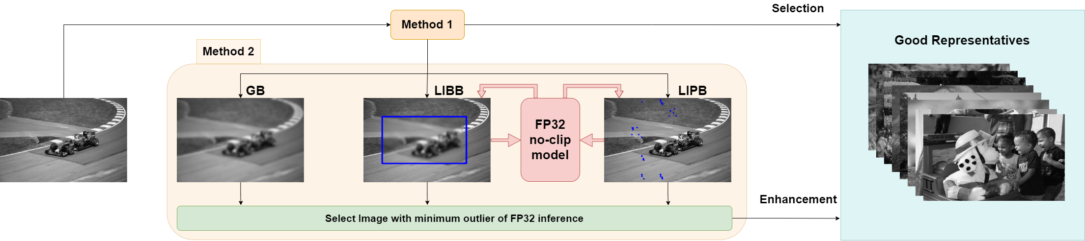
Figure 5: Workflow of CFQP.

5 Results

We provide the results of our proposed work in Table 5, 7, and Figure 6, 7, 8. Our extensive experiments reveal that CFQP performs as intended and as discussed in previous sections.

	XCAT			ABPN			ESPCN			FSRCNN			RFDNNet
	✓	✗	$\uparrow$	✓	✗	$\uparrow$	✓	✗	$\uparrow$	✓	✗	$\uparrow$	✓	✗	$\uparrow$
CPU	458	379	20.8%	779	715	9.0%	328	213	54.0%	1610	1564	2.9%	904	810	11.6%
TFLite GPU	460	445	3.4%	790	781	1.2%	342	339	0.9%	667	554	20.4%	484	465	4.1%
Android NNAPI	451	416	8.4%	254	197	28.9%	187	155	20.6%	309	275	12.4%	600	545	10.1%
Qualcomm Hexagon	377	338	11.5%	178	150	18.7%	113	91	24.2%	1207	1206	0%	519	498	4.2%
Qualcomm QNN GPU	502	375	33.9%	772	728	6.0%	322	213	51.2%	1605	1552	3.4%	917	836	9.7%

Table 5: Average runtime (ms) on different backends for clipped (✓) INT8 models, no-clip INT8 (✗) models, and the improvement over no-clip INT8 models ($\uparrow$). We achieve 14.86% $\uparrow$ on average for all models. The input tensor dimension is 640x360, and the inferences are repeated 20 times. [Ignatov et al.(2019)Ignatov, Timofte, Kulik, Yang, Wang, Baum, Wu, Xu, and Van Gool] is used for inference on Xiaomi RedMi Note 8 mobile phone.

Models	Test sets
	Set5	Set14	BSD100	Urban100
XCAT	32.98/32.86	29.41/29.36	28.38/28.34	26.30/26.20
ABPN	33.18/33.00	29.51/29.52	28.51/28.43	26.56/26.42
ESPCN	32.23/32.72	28.89/28.85	28.04/28.43	25.56/25.86
FSRCNN	32.83/32.72	29.25/29.31	28.27/28.24	26.01/25.96
RFDNNet	32.97/32.27	29.33/29.35	28.39/28.67	26.24/26.04

Table 6: PSNR of FP32 models on different train sets (DIV2K/Flickr).

$\Delta$	INT8	INT8*	$\Delta$	INT8	INT8*
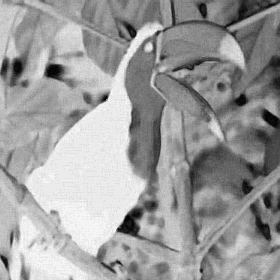
	21.21/0.896	33.40/0.958		24.64/0.914	33.00/0.948

Figure 6: No-clip XCAT PSNR/SSIM results. * whose RI is undergone our pipeline yield better results. Notice the color inconsistencies due to unaltered bad RI (DIV2K train #736).

Test	Models	Clipped		No-Clip
		M1	M1	M1	M1	$\text{\cancel{M1}}\rightarrow\text{M2}$
Set5	XCAT	32.329 (15)	32.310 (785)	32.640 (15)	28.409 (785)	32.346 (785)
	ABPN	32.492 (15)	32.526 (785)	32.975 (15)	28.360 (785)	32.276 (785)
	ESPCN	31.139 (8)	30.855 (792)	31.501 (8)	26.213 (792)	31.758 (792)
	FSRCNN	31.232 (13)	31.124 (787)	31.529 (13)	27.178 (787)	31.439 (787)
	RFDNNet	32.167 (7)	31.766 (793)	32.079 (7)	27.012 (793)	31.798 (793)
Set14	XCAT	28.956 (15)	28.890 (785)	29.131 (15)	26.516 (785)	28.910 (785)
	ABPN	29.042 (15)	28.956 (785)	29.360 (15)	26.380 (785)	28.906 (785)
	ESPCN	28.239 (8)	28.616 (792)	28.478 (8)	25.089 (792)	28.649 (792)
	FSRCNN	28.096 (13)	28.149 (787)	28.241 (13)	25.539 (787)	28.271 (787)
	RFDNNet	29.058 (7)	28.906 (793)	28.877 (7)	25.605 (793)	28.748 (793)
BSD100	XCAT	28.094 (15)	28.126 (785)	28.216 (15)	25.907 (785)	28.126 (785)
	ABPN	28.165 (15)	28.196 (785)	28.408 (15)	26.069 (785)	28.150 (775)
	ESPCN	27.494 (8)	27.821 (792)	27.684 (8)	24.960 (792)	27.843 (792)
	FSRCNN	27.611 (13)	27.736 (787)	27.723 (13)	25.452 (787)	27.785 (787)
	RFDNNet	28.231 (7)	28.149 (793)	28.165 (7)	25.459 (793)	28.073 (793)
Urban100	XCAT	25.964 (15)	25.967 (785)	26.137 (15)	24.328 (785)	25.845 (775)
	ABPN	26.197 (15)	26.261 (785)	26.440 (15)	24.318 (785)	25.943 (775)
	ESPCN	25.211 (8)	25.104 (792)	25.349 (8)	23.056 (792)	25.448 (792)
	FSRCNN	25.410 (13)	25.444 (787)	25.420 (13)	23.537 (787)	25.397 (787)
	RFDNNet	26.046 (7)	25.922 (793)	25.971 (7)	23.619 (793)	25.815 (793)

Table 7: Average of differently quantized models with the images (good) in Method 1 (M1), images which are rejected (bad) by Method 1 (M1) , and the bad images improved by our Method 2 ($\text{\cancel{M1}}\rightarrow\text{M2}$) on 4 different validation sets. Each PNSR entry is the average of (n) differently quantized models, where their representative images are chosen from DIV2K training set (800).

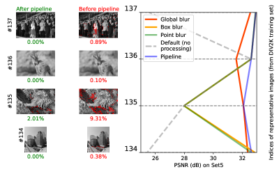
Figure 8: PSNR on Set5 for no-clip XCAT for the possible RI selections. The best augmentation methods for the corresponding RI and the FP32 output responses are also provided. Our proposed pipeline gives us the best augmentation selections for RI on average.

6 Conclusion

In this work, we showed the importance of representative image selection for PTQ. Specifically, we have presented a novel RI selection and enhancement pipeline (CFQP) for PTQ of no-clip SR networks. It is based on reducing outlier values in images with the selected image augmentation methods, making every image in a training dataset a candidate for RI. Results reveal that our proposed method on no-clip INT8 models outperforms clipped INT8 model counterparts regarding visual quality and provides a faster inference due to clipping removal. For future work, we aim to work on creating good representative images using generative networks.

References

- [Agustsson and Timofte(2017)] Eirikur Agustsson and Radu Timofte. Ntire 2017 challenge on single image super-resolution: Dataset and study. In The IEEE Conference on Computer Vision and Pattern Recognition (CVPR) Workshops, July 2017.
- [Ayazoglu(2021)] Mustafa Ayazoglu. Extremely lightweight quantization robust real-time single-image super resolution for mobile devices. In Proceedings of the IEEE/CVF Conference on Computer Vision and Pattern Recognition (CVPR) Workshops, pages 2472–2479, June 2021.
- [Ayazoglu and Bilecen(2023)] Mustafa Ayazoglu and Bahri Batuhan Bilecen. Xcat - lightweight quantized single image super-resolution using heterogeneous group convolutions and cross concatenation. In Computer Vision – ECCV 2022 Workshops, pages 475–488, Cham, 2023. Springer Nature Switzerland.
- [Bevilacqua et al.(2012)Bevilacqua, Roumy, Guillemot, and line Alberi Morel] Marco Bevilacqua, Aline Roumy, Christine Guillemot, and Marie line Alberi Morel. Low-complexity single-image super-resolution based on nonnegative neighbor embedding. In Proceedings of the British Machine Vision Conference, pages 135.1–135.10. BMVA Press, 2012.
- [Choi et al.(2018)Choi, Wang, Venkataramani, Chuang, Srinivasan, and Gopalakrishnan] Jungwook Choi, Zhuo Wang, Swagath Venkataramani, Pierce I-Jen Chuang, Vijayalakshmi Srinivasan, and Kailash Gopalakrishnan. PACT: parameterized clipping activation for quantized neural networks. CoRR, 2018.
- [Conde et al.(2023)Conde, Zamfir, Timofte, et al.] Marcos V Conde, Eduard Zamfir, Radu Timofte, et al. Efficient deep models for real-time 4k image super-resolution. ntire 2023 benchmark and report. In Proceedings of the IEEE/CVF Conference on Computer Vision and Pattern Recognition, 2023.
- [Dong et al.(2016)Dong, Loy, and Tang] Chao Dong, Chen Change Loy, and Xiaoou Tang. Accelerating the super-resolution convolutional neural network. In Bastian Leibe, Jiri Matas, Nicu Sebe, and Max Welling, editors, Computer Vision – ECCV 2016, pages 391–407, Cham, 2016. Springer International Publishing.
- [Du et al.(2021)Du, Liu, Tang, and Wu] Zongcai Du, Jie Liu, Jie Tang, and Gangshan Wu. Anchor-based plain net for mobile image super-resolution. In Proceedings of the IEEE/CVF Conference on Computer Vision and Pattern Recognition (CVPR) Workshops, pages 2494–2502, June 2021.
- [Haichao Yu(2021)] Humphrey Shi Haichao Yu, Linjie Yang. Is in-domain data really needed? a pilot study on cross-domain calibration for network quantization. In Proceedings of the IEEE/CVF Conference on Computer Vision and Pattern Recognition, 2021.
- [Ignatov and Timofte(2023)] Andrey Ignatov and Radu Timofte. Efficient and accurate quantized image super-resolution on mobile npus, mobile ai & aim 2022 challenge: Report. In Computer Vision – ECCV 2022 Workshops, pages 92–129, Cham, 2023. Springer Nature Switzerland.
- [Ignatov et al.(2019)Ignatov, Timofte, Kulik, Yang, Wang, Baum, Wu, Xu, and Van Gool] Andrey Ignatov, Radu Timofte, Andrei Kulik, Seungsoo Yang, Ke Wang, Felix Baum, Max Wu, Lirong Xu, and Luc Van Gool. Ai benchmark: All about deep learning on smartphones in 2019, 10 2019.
- [Ignatov et al.(2021)Ignatov, Timofte, Denna, and Younes] Andrey Ignatov, Radu Timofte, Maurizio Denna, and Abdel Younes. Real-time quantized image super-resolution on mobile npus, mobile ai 2021 challenge: Report. In Proceedings of the IEEE/CVF Conference on Computer Vision and Pattern Recognition (CVPR) Workshops, pages 2525–2534, June 2021.
- [Li et al.(2022)Li, Zhang, Timofte, and Gool] Yawei Li, Kai Zhang, Radu Timofte, and Van Gool. Ntire 2022 challenge on efficient super-resolution: Methods and results. In Proceedings of the IEEE/CVF Conference on Computer Vision and Pattern Recognition (CVPR) Workshops, pages 1062–1102, June 2022.
- [Liu et al.(2020)Liu, Tang, and Wu] Jie Liu, Jie Tang, and Gangshan Wu. Residual feature distillation network for lightweight image super-resolution, 2020.
- [Ruonan Yu(2023)] Xinchao Wang Ruonan Yu, Songhua Liu. Dataset distillation: A comprehensive review. In IEEE Transactions on Pattern Analysis and Machine Intelligence, 2023.
- [Shi et al.(2016)Shi, Caballero, Huszar, Totz, Aitken, Bishop, Rueckert, and Wang] Wenzhe Shi, Jose Caballero, Ferenc Huszar, Johannes Totz, Andrew P. Aitken, Rob Bishop, Daniel Rueckert, and Zehan Wang. Real-time single image and video super-resolution using an efficient sub-pixel convolutional neural network. In Proceedings of the IEEE Conference on Computer Vision and Pattern Recognition (CVPR), June 2016.
- [Yuan et al.(2023)Yuan, Liu, Wu, Yang, Wu, Sun, Liu, Wang, and Wu] Zhihang Yuan, Jiawei Liu, Jiaxiang Wu, Dawei Yang, Qiang Wu, Guangyu Sun, Wenyu Liu, Xinggang Wang, and Bingzhe Wu. Benchmarking the reliability of post-training quantization: a particular focus on worst-case performance, 2023.
- [Zamfir et al.(2023)Zamfir, Conde, and Timofte] Eduard Zamfir, Marcos V Conde, and Radu Timofte. Towards real-time 4k image super-resolution. In Proceedings of the IEEE/CVF Conference on Computer Vision and Pattern Recognition, 2023.
- [Zhang et al.(2022)Zhang, Gao, Fan, Zhao, Yang, and Yan] Zhao Zhang, Yangcheng Gao, Jicong Fan, Zhongqiu Zhao, Yi Yang, and Shuicheng Yan. SelectQ: Calibration Data Selection for Post-Training Quantization, 11 2022.
- [Zhuo et al.(2022)Zhuo, Chen, Ramakrishnan, Chen, Feng, Lin, Zhang, and Shen] Shaojie Zhuo, Hongyu Chen, Ramchalam Kinattinkara Ramakrishnan, Tommy Chen, Chen Feng, Yicheng Lin, Parker Zhang, and Liang Shen. An empirical study of low precision quantization for tinyml, 2022.