Self-consistent autocorrelation for finite-area bias correction in roughness measurement

Abstract

Scan line levelling, a ubiquitous and often necessary step in AFM data processing, can cause a severe bias on measured roughness parameters such as mean square roughness or correlation length. Although bias estimates have been formulated, they aimed mainly at assessing the severity of the problem for individual measurements. Practical bias correction methods are still missing. This work exploits the observation that the bias of autocorrelation function (ACF) can be expressed in terms of the function itself, permitting a self-consistent formulation. From this two correction approaches are developed, both with the aim to obtain convenient formulae which can be easily applied in practice. The first modifies standard analytical models of ACF to incorporate, in expectation, the bias and thus actually match the data the models are used to fit. The second inverts the relation between true and estimated ACF to realise a model-free correction. Both are tested using simulated and experimental data and found effective.

Keywords: Scanning Probe Microscopy, roughness, autocorrelation, bias

1 Introduction

Recently a couple of works drew attention to how roughness measurement by atomic force microscopy (AFM) are impacted by levelling/background subtraction [1, 2], in particular line levelling, a ubiquitous and often necessary step in AFM data processing [3, 4, 5, 6]. The classic results for the effect of mean value subtraction on statistical quantities [7, 8, 9] were generalised in a theoretical framework covering many common levelling methods. The mean square roughness $\sigma$, as well as many other quantities, becomes biased. For 1D data and 1D scan line levelling the bias of estimate $\hat{\sigma}$ can be written (in expectation):

$$\mathrm{E}[\hat{\sigma}^{2}]=\sigma^{2}-2\int_{0}^{1}G(tL)\,C(t)\,\rmd t\;.$$ (1)

Function $G$ is the true autocorrelation function (ACF) of the roughness and $C$ a complicated function capturing correlation/spectral properties of the specific levelling method. The second term expresses the measurement bias, which can often be severe [8, 1, 2]. Explicit expressions are known for several common levelling methods and autocorrelation function forms. [1] It should be noted that is more correct to call $G$ the autocovariance function and reserve the term autocorrelation for the function normalised to variance, but both are commonly used. The bias problem is not unique to AFM and profilometry data levelling. Similar problems occur for autocovariance function estimation from locally smoothed (detrended) data [10, 11].

Ultimately, the bias and variance depend on the ratio $\alpha=T/L$ of correlation length $T$ and scan line length $L$. The bias further increases with ‘aggressivity’ of the levelling procedure [8, 1]. The ratio $\alpha$ must be kept small for reliable results. If scan line levelling and similar 1D corrections are applied to images the error is proportional to $\alpha$ (not $\alpha^{2}$ as one might assume for 2D image data), which can be difficult to keep sufficiently small. Even when scan lines are not levelled explicitly, the computation of 1D ACF imposes the condition of zero mean value on image rows, corresponding to degree-0 polynomial levelling. The length $L$ is, sadly, also often not set deliberately but instead to what ‘feels right’ [2]. This then translates to $\alpha$ which is way too large—sometimes far beyond instrumental constraints. Reported results are then unnecessarily skewed. Bias estimation procedures have been proposed, either simple and coarse [2] or more detailed [1], allowing one to check whether it is within reasonable bounds. The simplest (and coarsest) estimate of relative bias of $\hat{\sigma}$ is $-n\alpha$, where $n$ is the number of terms in the scan line levelling polynomial, usually equal to its degree plus one.

Unfortunately, all the estimates suffer from a chicken and egg problem. They require knowing the correlation length $T$, or even the form of the ACF, which are not known a priori. They should be the outputs of our measurement. Therefore, they must be estimated from experimental data, and these estimates are again biased. The experimental $T$ (denoted $\hat{T}$) is underestimated because the entire ACF is affected in a similar manner as $\sigma^{2}$, as illustrated in figure 1. Consequently, although such estimates can help with judging the bias for a particular measurement or guide towards a better choice of scanning parameters, they cannot be applied in a logically consistent manner. They are thus of limited use for actual correction of the biased results. Clearly, the problem is not yet satisfactorily solved. In order to deal with the bias pervading all the roughness parameters we need a self-consistent method which does not require a priori knowledge of the result. It should also be convenient to have practical impact and allow wide adoption. Here we aim to provide this missing piece.

Figure 1: The effect of scan line polynomial levelling using polynomials of various degrees on the estimated ACF. The beginning of the curve (small distances) is biased, whereas for larger distances the ACF estimate is not converged and exhibits oscillations [8].

The overall plan is fairly straightforward. We being from the observation that the value of ACF at zero is $\sigma^{2}$, that is $\sigma^{2}=G(0)$. Formula (1) can thus be also written

$$\mathrm{E}[\hat{G}(0)]=G(0)-2\int_{0}^{1}G(tL)\,C(t)\,\rmd t\;.$$ (2)

The second (bias) term is linear in $G$. Suppose an expression of the same form could be obtained for $G$ as a whole (we show later that it is indeed the case)

$$\mathrm{E}[\hat{G}]=G-RG\;.$$ (3)

Here $R$ is a linear operator expressing the bias, now of the entire ACF. It again captures the properties of the specific levelling procedure. Expression (3) ties self-consistently together the true and estimated ACF. We can say that the ACF knows about its own bias. The relation can be formally inverted

$$G=(1-R)^{-1}\mathrm{E}[\hat{G}]\;,$$ (4)

yielding unbiased $G$ from the biased estimate $\hat{G}$ (in expectation). This is the adventurous option—it is not immediately obvious such inversion would be numerically feasible.

The conservative option is to employ expression (3) directly. Assume, for instance, that the roughness is Gaussian. The true ACF has then the form

$$G_{\mathrm{Gauss}}(\tau)=\sigma^{2}\exp\left(-\frac{\tau^{2}}{T^{2}}\right)\;.$$ (5)

Conventionally, we fit the experimental ACF $\hat{G}(\tau)$ with the ideal model $G_{\mathrm{Gauss}}(\tau)$ with $\sigma$ and $T$ as free parameters. But it is clearly the wrong model. It does not describe the experimental ACF, which never conforms to the theoretical form. The correct model is

$$G_{\mathrm{Gauss}}(\tau)-RG_{\mathrm{Gauss}}(\tau)$$ (6)

and can be obtained by applying $R$ to $G_{\mathrm{Gauss}}(\tau)$.

The questions are what is the form or operator $R$, whether $R$ and $(1-R)^{-1}$ can be reasonably evaluated and how well the bias correction works in practice. They are answered in the following sections. The general expression for $R$ is derived in section 2, which the reader can skip on the first reading. Section 3 provides elementary formulae and procedures for practical bias correction and section 4 tests their effectiveness using simulations and real AFM data.

2 Bias of ACF after levelling

The calculation of $R$ follows the general scheme and notation introduced in Ref. 1 (sections 3.1 and 3.3), including treating the data as continuous functions. Since scan line levelling is the dominant source of bias even for image data [2], we consider the 1D case. Denote $\varphi_{j}$ orthonormal basis functions used for background subtraction by linear fitting, with $j$ distinguishing the functions. If $\varphi_{j}$ are polynomials then $j\in\{0,1,2,\dots n-1\}$ is their degree, but the index may not be a simple integer in other cases. Summations over $j$ are, therefore, written below only formally.

Levelled data are computed by subtracting the projection onto the span of $\varphi_{j}$

$$\hat{z}(x)=z(x)-\sum_{j}a_{j}\varphi_{j}(x)\;,$$ (7)

with coefficients $a_{j}$ equal to the dot products

$$a_{j}=\int_{0}^{L}z(x)\,\varphi_{j}(x)\,\rmd x\;.$$ (8)

The ACF is estimated as

$$\hat{G}(\tau)=\frac{1}{L-\tau}\int_{0}^{L-\tau}\hat{z}(x)\,\hat{z}(x+\tau)\,\rmd x\;.$$ (9)

Substituting expressions (7) into (9) gives for $\hat{G}(\tau)$

$$\frac{1}{L-\tau}\int_{0}^{L-\tau}\left[z(x)-\sum_{j}a_{j}\varphi_{j}(x)\right]\left[z(x+\tau)-\sum_{k}a_{k}\varphi_{k}(x+\tau)\right]\rmd x\;,$$ (10)

which can be expanded into four terms corresponding to the combinations of $z$ and $\varphi$:

$$\hat{G}(\tau)=\hat{G}_{1}(\tau)-\hat{G}_{2}(\tau)-\hat{G}_{3}(\tau)+\hat{G}_{4}(\tau)\;.$$ (11)

Taking expectations,

$$\eqalign{\mathrm{E}[\hat{G}_{1}(\tau)]&=G(\tau)\cr\mathrm{E}[\hat{G}_{2}(\tau)]&=\frac{1}{L-\tau}\sum_{j}\int_{0}^{L-\tau}\int_{0}^{L}G(x^{\prime}-x+\tau)\,\varphi_{j}(x)\,\varphi_{j}(x^{\prime})\,\rmd x^{\prime}\,\rmd x\cr\mathrm{E}[\hat{G}_{3}(\tau)]&=\frac{1}{L-\tau}\sum_{k}\int_{0}^{L-\tau}\int_{0}^{L}G(x^{\prime}-x)\,\varphi_{k}(x+\tau)\,\varphi_{j}(x^{\prime})\,\rmd x^{\prime}\,\rmd x\cr\mathrm{E}[\hat{G}_{4}(\tau)]&=\frac{1}{L-\tau}\sum_{j,k}\left[\int_{0}^{L}\int_{0}^{L}G(x^{\prime\prime}-x^{\prime})\,\varphi_{k}(x^{\prime})\,\varphi_{j}(x^{\prime\prime})\,\rmd x^{\prime}\,\rmd x^{\prime\prime}\right.\cr&\hphantom{=\frac{1}{L-\tau}\sum[}\times\left.\int_{0}^{L-\tau}\varphi_{j}(x)\varphi_{k}(x+\tau)\,\rmd x\right]\;,}$$ (12)

where we utilised the linearity of expectation and that for any $a$ and $b$

$$\mathrm{E}[z(a)z(b)]=G(b-a)=G(a-b)\;.$$ (13)

In a similar manner as in formula (1) for the bias of $\sigma^{2}$, one term (here $\mathrm{E}[\hat{G}_{1}]$) gives the unbiased $G(\tau)$ and the remaining terms combine to give the bias $RG(\tau)$.

2.1 Linear operator $R$

In principle, formulae (12) can already be considered a representation of the operator $R$. However, it is more natural (and useful) to write it explicitly

$$\mathrm{E}[\hat{G}(\tau)]=G(\tau)-\int_{0}^{L}R(\tau,u)\,G(u)\,\rmd u\;.$$ (14)

Meaning in $\mathrm{E}[\hat{G}_{2}(\tau)]$ we must set $u=x^{\prime}-x+\tau$, transform the domain of integration (which splits the integral into three) and obtain

$$\eqalign{\mathrm{E}[\hat{G}_{2}(\tau)]=\frac{1}{L-\tau}\sum_{j}\Bigl{[}\Bigr{.}&\int_{0}^{L-\tau}G(u)\,c_{j,[0,L-\tau-u]}(\tau+u)\,\rmd u\cr&+\int_{0}^{\tau}G(u)\,c_{j,[0,L-\tau]}(\tau-u)\,\rmd u\cr&+\int_{\tau}^{L}G(u)\,c_{j,[u-\tau,L-\tau]}(\tau-u)\,\rmd u\Bigl{.}\Bigr{]}\;.}$$ (15)

The symmetry of $G$ was utilised to ensure its argument is always positive and thus from interval $[0,L]$. Functions $c_{j}$ again express the correlation properties of $\varphi_{j}$, in analogy to Ref. 1. However, as the various integrals are over different subintervals of $[0,L]$ they are more complicated here, defined

$$c_{j,[a,b]}(\delta)=\int_{a}^{b}\varphi_{j}(x)\,\varphi_{j}(x+\delta)\,\rmd x\;.$$ (16)

Finally, in order to transform the expression to the form (14), we replace the integration limits for $u$ using the indicator function

$$\chi_{[a,b]}(x)=\cases{1&if $a\leq x\leq b$\cr 0&otherwise}$$ (17)

resulting in

$$\eqalign{\mathrm{E}[\hat{G}_{2}(\tau)]=\frac{1}{L-\tau}\int_{0}^{L}G(u)\sum_{j}\Bigl{[}\Bigr{.}&\chi_{[0,L-\tau]}(u)\,c_{j,[0,L-\tau-u]}(\tau+u)\cr&+\chi_{[0,\tau]}(u)\,c_{j,[0,L-\tau]}(\tau-u)\cr&+\chi_{[\tau,L]}(u)\,c_{j,[u-\tau,L-\tau]}(\tau-u)\Bigl{.}\Bigr{]}\,\rmd u\;.}$$ (18)

The term in square brackets is one piece of $R(\tau,u)$ in the form required by (14)—the one corresponding to $\hat{G}_{2}$. The second piece, corresponding to $\hat{G}_{3}$, is obtained using the same steps. The last piece contains integrals combining $\varphi_{j}$ and $\varphi_{k}$ for $j\neq k$ that cannot be expressed using (16). If we define

$$c_{j,k,b}(\delta)=\int_{0}^{b}\varphi_{j}(x)\,\varphi_{k}(x+\delta)\,\rmd x\;.$$ (19)

it can be written

$$\mathrm{E}[\hat{G}_{4}(\tau)]=\frac{1}{L-\tau}\int_{0}^{L}G(u)\sum_{j,k}[c_{j,k,L-u}(u)+c_{k,j,L-u}(u)]c_{j,k,L-\tau}(\tau)]\,\rmd u$$ (20)

Therefore, the final expression for $R(\tau,u)$ is

$$\eqalign{R(\tau,u)&=\frac{1}{L-\tau}\sum_{j}\Bigl{[}\chi_{[0,L-\tau]}(u)\bigl{(}c_{j,[0,L-\tau-u]}(\tau+u)+c_{j,[\tau+u,L]}(-\tau-u)\bigr{)}\Bigr{.}\cr&\hphantom{=\frac{1}{L-\tau}\sum}+\chi_{[0,\tau]}(u)\bigl{(}c_{j,[0,L-\tau]}(\tau-u)+c_{j,[\tau,L]}(u-\tau)\bigr{)}\cr&\hphantom{=\frac{1}{L-\tau}\sum}+\chi_{[\tau,L]}(u)\bigl{(}c_{j,[u-\tau,L-\tau]}(\tau-u)+c_{j,[\tau,L+\tau-u]}(u-\tau)\bigr{)}\Bigl{.}\Bigr{]}\cr&\hphantom{=}-\frac{1}{L-\tau}\sum_{j,k}\bigl{[}c_{j,k,L-u}(u)+c_{k,j,L-u}(u)\bigr{]}c_{j,k,L-\tau}(\tau)}$$ (21)

2.2 Polynomial levelling

A polynomial basis $\varphi_{j}$ has symmetries which can be used simplify $R(\tau,u)$ somewhat. We first note that the expression is not unwieldy because we failed to express it more elegantly. The operator is inherently complicated, with a number of discontinuities in the derivative. Even for mean value subtraction, when the single basis function $\varphi_{0}$ is a constant, we get

$$R_{0}(\tau,u)=\frac{2}{L}\left[\chi_{[0,L-\tau]}(u)\frac{L-\tau-u}{L-\tau}+\chi_{[0,\tau]}(u)\frac{u-\tau}{L-\tau}+\frac{(L-u)\tau}{L(L-\tau)}\right]\;,$$ (22)

illustrated in figure 2. Although only function values for small $\tau$ and $u$ are important and some of the discontinuities do not affect expansions for small $\tau$ and $u$, $R(\tau,u)$ is not totally differentiable at $(0,0)$. A small-$\tau$ approximation of the entire integral in (14) is possible only because the integral is a smoother function than $R(\tau,u)$ itself.

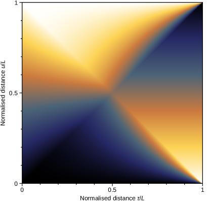
Figure 2: Linear operator $R_{0}(\tau,u)$ for mean value subtraction, normalised to $L$ (equivalent to putting $L=1$). The false colour scale corresponds to the interval $[0,2]$.

For general polynomials, we note that Legendre polynomials $\mathrm{P}_{n}(x)$ on interval $[-1,1]$ are either even or odd, $\mathrm{P}_{n}(-x)=(-1)^{n}\mathrm{P}_{n}(x)$. For the orthonormal basis functions on $[0,L]$ it translates to

$$\varphi_{j}(L-x)=(-1)^{j}\varphi(x)\;.$$ (23)

From this we can easily see that

$$c_{j,k,L-\tau}(\tau)=(-1)^{j+k}c_{k,j,L-\tau}(\tau)\;.$$ (24)

Terms with $j+k$ odd can be omitted as they mutually cancel. And for $j+k$ even only terms with $j<k$ can be kept, multiplied by 2. Together with the relation $c_{j,j,b}=c_{j,[0,b]}$, permitting rewriting terms with $j=k$, these rules eliminate most of the terms in the second summation in (21). In fact, for degree 1 no such term remains, giving

$$\eqalign{R_{1}(\tau,u)&=\frac{1}{L-\tau}\sum_{j=0}^{1}\Bigl{[}\chi_{[0,L-\tau]}(u)\bigl{(}c_{j,[0,L-\tau-u]}(\tau+u)+c_{j,[\tau+u,L]}(-\tau-u)\bigr{)}\Bigr{.}\cr&\hphantom{=\frac{1}{L-\tau}\sum}+\chi_{[0,\tau]}(u)\bigl{(}c_{j,[0,L-\tau]}(\tau-u)+c_{j,[\tau,L]}(u-\tau)\bigr{)}\cr&\hphantom{=\frac{1}{L-\tau}\sum}+\chi_{[\tau,L]}(u)\bigl{(}c_{j,[u-\tau,L-\tau]}(\tau-u)+c_{j,[\tau,L+\tau-u]}(u-\tau)\bigr{)}\cr&\hphantom{=\frac{1}{L-\tau}\sum}-2c_{j,[0,L-u]}(u)c_{j,[0,L-\tau]}(\tau)\Bigl{.}\Bigr{]}\cr}$$ (25)

A similar simplification is possible for other bases formed by even and odd functions $\varphi_{j}$, for instance sines and cosines, although the indexing by $j$ may differ (and sines and cosines are more natural to handle in the frequency domain). However, the small-$(\tau,u)$ expansion for a specific basis is still tedious and better evaluated using symbolic algebra software.

Maxima [12] was used to obtain the practical formulae summarised in the following section. The expansions were terminated at $\alpha^{2}$ terms. The first reason is that preliminary numerical experiments showed that the leading $\alpha^{1}$ terms is not always sufficient and without the second term there is a tendency to overcorrection. The general form of $\sigma^{2}$ bias for polynomial levelling contains only even-power terms after $\alpha^{2}$ (equation (27) in Ref. 1). Therefore, there is no third order term in the expansion and higher powers are negligible. Finally, the low smoothness of $R$ at zero means that more accurate expansions would not be, in general, Taylor-like and would have to include more complicated ACF-specific terms. For this reason it is advantageous to express analytical models of ACF in terms of $\alpha=T/L$ and $s=\tau/T$ as it makes them smoother functions. In model-free inversion there is no $T$. Therefore, the formulation has to be done in terms of $t=\tau/L$ instead of $s$.

3 Practical formulae

3.1 Corrected models

The (biased) discrete ACF is estimated from data values $z_{k}$ [8]

$$\hat{G}_{k}=\frac{1}{N-k}\sum_{m=0}^{N-1-k}z_{m}z_{m+k}\;,$$ (26)

where $\tau=k\Delta_{x}$ if $\Delta_{x}$ is the sampling step. It is fitted by an ACF model function. Simple models have only two free parameters, $\sigma$ and $T$. The classic Gaussian ACF model (5) and analogous exponential model

$$G_{\mathrm{exp}}(\tau)=\sigma^{2}\exp\left(-\frac{\tau}{T}\right)=\sigma^{2}\rme^{-s}\;.$$ (27)

are replaced with the leading terms of $(G-BG)(\tau)$ expanded for small $\alpha$ and $\tau$. In particular, the Gaussian model is replaced with

$$G_{\mathrm{Gauss}}^{\mathrm{bias}}(\tau)=\sigma^{2}\left[\rme^{-s^{2}}(1+n^{2}\alpha^{2})-\sqrt{\pi}n\alpha+\sqrt{\pi}n\alpha^{2}s\bigl{(}n\mathop{\mathrm{erf}}(s)-1\bigr{)}\right]$$ (28)

and the exponential model with

$$G_{\mathrm{exp}}^{\mathrm{bias}}(\tau)=\sigma^{2}\left[\rme^{-s}(1+2n^{2}\alpha^{2})-2n\alpha+2n(n-1)\alpha^{2}s\right]\;.$$ (29)

where $s=\tau/T$, $\alpha=T/L$ and erf denotes the error function (antiderivative of Gaussian). If evaluation of special functions is not possible or desirable erf can be replaced for instance by a Padé-style approximation as it only occurs in the second order term.

The superscript ^bias indicates the models take into account the bias of the data (26) they are used to fit. Models (28) and (29) should be fitted from zero to approximately the first zero crossing, i.e. up to the first $k$ for which $G_{k}<0$. The biased models do not have any additional free parameters. Nevertheless, they contain two additional inputs, the profile or scan line length $L$ and the number of terms $n$ of the line levelling polynomial—which is one plus its degree. The full profile length must be entered as $L$, not the length of ACF data which are often cut to a shorter interval of $\tau$.

3.2 Model-free inversion

For an ACF of an unknown form, although still quickly monotonically decreasing, we note that the leading terms in an $(\alpha,t)$ expansion originate from integrals

$$M_{0}[G]=\int_{0}^{\infty}G(u)\,\rmd u\quad\hbox{and}\quad M_{1}[G]=\int_{0}^{\infty}uG(u)\,\rmd u\;.$$ (30)

For the discrete experimental ACF $\hat{G}_{k}$ it leads to the equations

$$\hat{G}_{k}=G^{\mathrm{c}}_{k}-\frac{2n}{N}\left(1+\frac{k}{N}\right)\sum_{m=0}^{K-1}G^{\mathrm{c}}_{m}+\frac{2n^{2}}{N^{2}}\left(1+\frac{2k}{N}\right)\sum_{m=0}^{K-1}mG^{\mathrm{c}}_{m}\;.$$ (31)

This is a set of $K$ linear equations for corrected $G^{\mathrm{c}}_{m}$ with $m=0,1,2,\dots,K-1$. Index $K$ represents a cut-off after which the function is assumed to be negligible or the data not usable, i.e. again around the first zero crossing.

Although the equations could also be written in a explicitly matrix-like form

$$\sum_{m=0}^{K-1}R_{k,m}G^{\mathrm{c}}_{m}=\hat{G}_{k}$$ (32)

with

$$R_{k,m}=\delta_{km}-\frac{2n}{N}\left(1+\frac{k}{N}\right)+\frac{2n^{2}}{N^{2}}\left(1+\frac{2k}{N}\right)m\;,$$ (33)

the form (31) shows that in this case the matrix multiplication, which would normally require $\Omega(K^{2})$ operations, reduces to two much simpler summations requiring only $\Omega(K)$ operations because the sums

$$S_{0}[G^{\mathrm{c}}]=\sum_{m=0}^{K-1}G^{\mathrm{c}}_{m}\quad\hbox{and}\quad S_{1}[G^{\mathrm{c}}]=\sum_{m=0}^{K-1}mG^{\mathrm{c}}_{m}$$ (34)

do not depend on $k$. Therefore, they only have to be computed once:

$$\sum_{m=0}^{K-1}R_{k,m}G^{\mathrm{c}}_{m}=G^{\mathrm{c}}_{k}-\frac{2n}{N}\left(1+\frac{k}{N}\right)S_{0}[G^{\mathrm{c}}]+\frac{2n^{2}}{N^{2}}\left(1+\frac{2k}{N}\right)S_{1}[G^{\mathrm{c}}]\;.$$ (35)

The same holds for multiplication with $R^{\mathrm{T}}$ which simplifies to

$$\sum_{m=0}^{K-1}R^{\mathrm{T}}_{k,m}G^{\mathrm{c}}_{m}=G^{\mathrm{c}}_{k}-\frac{2n}{N}\left(1-\frac{kn}{N}\right)S_{0}[G^{\mathrm{c}}]-\frac{2n}{N^{2}}\left(1-\frac{2kn}{N}\right)S_{1}[G^{\mathrm{c}}]$$ (36)

The linear system

$$R^{\mathrm{T}}TG^{\mathrm{c}}=R^{\mathrm{T}}\hat{G}$$ (37)

has a positive definite matrix. Therefore, the method of conjugated gradients [13, 14] can be used to solve it quickly as all matrix multiplications (35) and (36) are computationally cheap. Starting from the initial estimate $G^{\mathrm{c}}_{k}=\hat{G}_{k}$, only a couple of iterations are required for convergence.

4 Numerical and experimental examples

4.1 Simulated data—Gaussian ACF

We first compare the performance of standard and biased Gaussian roughness models (5) and (28) using simulated data. Synthetic rough Gaussian surfaces were generated using the spectral method with $T=20\,\hbox{px}$. The correlation length is in the typical range for real AFM images, regardless of the physical dimensions of the scanned area. The mean square roughness $\sigma$ was set to 1 as it is only a scaling parameter. The image size varied from 100 px to 2000 px, corresponding to $\alpha$ from 0.01 to 0.2 (in the reverse order). The discrete ACF (26) was evaluated using the standard Fast Fourier Transform method, after levelling image rows using polynomials with degrees from 0 to 2.

The polynomial levelling was, of course, not actually necessary here because the simulated data were ideal and had neither tilt nor bow. It simulated the effect of preprocessing that would be applied to measured data. Tilt or bow could be added beforehand, but it would be pointless. The levelling would subtract them again, together with a part of the roughness—which is the effect we are studying.

Marquardt–Levenberg algorithm was used for the non-linear least squares fitting to obtain $\sigma$ and $T$. Both models were fitted to data up to the first zero crossing. The entire procedure was repeated with randomly generated Gaussian surfaces hundreds of times (with more repetitions for smaller images for which the variances are larger). The means and standard deviations are plotted in figure 3.

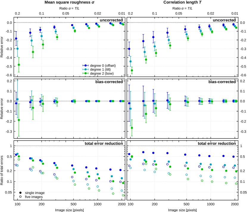
Figure 3: Comparison of fitting the biased Gaussian ACF model (28) with the standard one (5) (for correlation length of 20 px). Error bars represent single-image standard deviations. Results for different polynomial degrees are slightly offset horizontally for visual clarity.

The biased model (28) clearly succeeded at bias reduction. For both parameters and almost all image sizes the bias becomes so small that it is no longer an issue. The only exception is very small images which are only several correlation lengths large ($\alpha\lesssim 1/10$). Although bias usually still decreases, it is at the cost of considerably increased variance. Too much roughness information is missing in such small areas. Using them for roughness evaluation is just wrong and the correction cannot change it.

The correction generally trades the bias for variance, i.e. the parameters have larger variances than for the standard model. For reasonable $T/L$ the trade-off is advantageous. The total error $(\hbox{variance}+\hbox{bias}^{2})^{1/2}$ decreases as illustrated in the bottom row of figure 3. The improvement is more marked for $\sigma$ where it can be an order of magnitude, whereas for $T$ it ranges from about $2\times$ to $5\times$. The improvement is larger for higher polynomial degrees. It is because the bias is larger in absolute value, but of the same functional form. Hence, the same correction is able to deal with a larger bias.

Full circles in figure 3 correspond to the worst case scenario of a single-image roughness measurement. Multiple scans reduce the variance, the dominant contribution for the improved model, but do not help with bias, the dominant contribution for the standard one. This is illustrated in the plot of total error reduction for five-image evaluation (open circles).

4.2 Simulated data—inversion

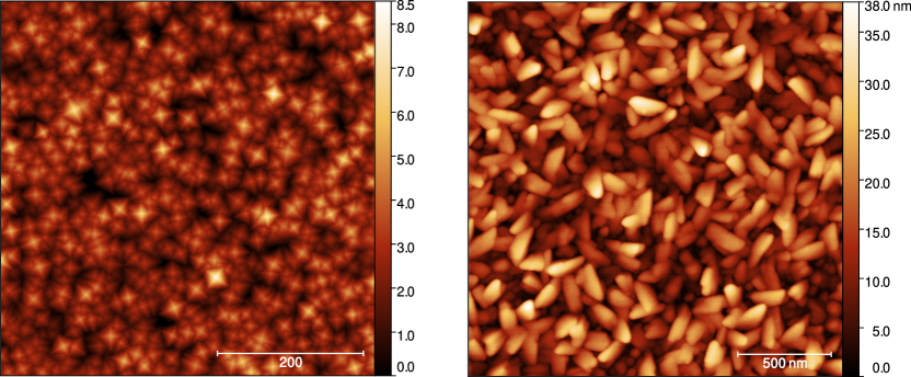
Figure 4: Small parts ($512\times 512$) of surfaces used in the model-free correction (inversion) examples. Left: simulated random pyramids. Right: polycrystalline SrO thin film.

For model-free correction (inversion) random pyramidal surfaces with an unknown ACF were generated using Gwyddion [15] Objects function which generates surfaces by sequential ‘extrusion’ [16]. The pyramids were randomly oriented and the pattern was large-scale isotropic. The generated images were $8000\times 8000$ pixels, corresponding to approximately 700 correlation lengths $(\alpha\approx 0.0015)$. A small ($512\times 512$) part of one such image is shown in figure 4. Smaller images of various sizes were again cut from the large base image and used to estimate the ACF.

The corrected ACF was computed by cutting $\hat{G}_{k}$ slightly beyond the first zero crossing (10 % farther) and solving the linear system (31) as described in section 3.2. Roughness parameters $\sigma$ and $T$ were again evaluated from both the biased and corrected ACF. In particular $\sigma$ was calculated from the relation $\sigma^{2}=G_{0}$ and $T$ as the distance at which the ACF first falls to $G_{0}/\rme$ ($\rme$ being Euler’s number). The $1/\rme\approx 0.368$ threshold is consistent with the analytic models (5) and (27), although it should be noted that roughness measurement standards often set the threshold differently, 0.2 being a common choice [17].

The comparison also requires true values of $\sigma$ and $T$. They were obtained using angularly averaged 2D ACF, which was averaged over all generated images. The data were artificial and did not contain any tilt, bow, sample bending or other type of background. Therefore, the only preprocessing necessary before the computation of 2D ACF was the subtraction of the mean value from the entire image. The relative bias introduced by this operation is of the order of $\alpha^{2}$ [8, 1], i.e. $<10^{-5}$ and thus negligible.

The results are plotted in figure 5. The overall trends are similar as for the modified Gaussian model fitting, but the accuracy improvements are more moderate. Although an improvement by factor of 2 is still not negligible, it is only observed for degree 2 levelling. For mean value subtraction the correction may not be worth the effort (at least with single-image evaluation) and can in fact even make the total error slightly larger. While $\sigma$ is corrected almost perfectly, $T$ appears slightly overcorrected, leaving a small bias and weakening the effectiveness, especially for large images where the error is already small. Multi-image evaluation (open circles) again increases the total error improvement.

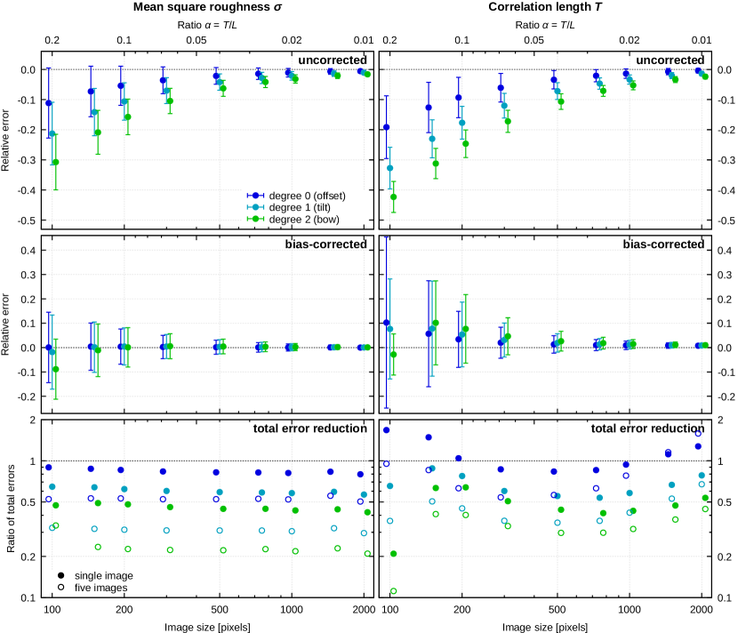
Figure 5: Comparison of roughness parameters $\sigma$ and $T$ obtained from uncorrected and model-free corrected ACF curves for a random pyramidal surface. Error bars represent single-image standard deviations. Results for different polynomial degrees are slightly offset horizontally for visual clarity.

We also tested how the correction depends on the ACF cut-off point by choosing the interval from 10% shorter to 40% longer than to the first zero crossing. The effect can be assessed using the accuracy of $\sigma$ and $T$ or differences between the corrected and true ACF curves. All the dependencies are generally quite flat and often without any clear trend. This is a reassuring result because it means the correction is not sensitive to the cut-off point precise location. As expected, for very tiny images (large $\alpha$) shortening the interval improves the accuracy somewhat. For large images (small $\alpha$) the trend was sometimes slightly opposite. Overall, however, cutting at the first zero crossing or moderately beyond it appeared to work well.

4.3 Rough thin film—inversion

A test with real rough surface would ideally be done with a sample whose ACF is precisely known. However, even standard rough samples do not have the ACF specified. Furthermore, the objective is to verify that the bias caused by limited area can be corrected. Meaning the resulting ACF is close to ACF which would be obtained by measuring a very large (or infinite) area. The same approach as in the previous section can thus be used. In fact, comparing measurements on small and huge areas allows us to study the effect in isolation—as opposed to comparison with a reference ACF where any observed difference could have a variety of possible causes.

An SrO thin film, prepared by atomic layer deposition, with large-scale uniformly and isotropically rough upper surface was chosen for the demonstration (see figure 4). The texture is formed by nanocrystals and is clearly non-Gaussian. Images were acquired using a Bruker Dimension Icon atomic force microscope in ScanAsyst mode with a standard ScanAsyst-air probe and scan rate of 0.2 Hz. In order to follow the 2D ACF route, a large image without scan line artefacts is necessary. The absence of scan line artefacts means 2D polynomial levelling is sufficient, leaving only bias proportional to $\alpha^{2}$ (or higher powers). A scan of area $12\times 12\,\hbox{\textmu m}^{2}$ with pixel resolution of $3072\times 3072$ was selected for the evaluation. The correlation length to scan size ratio was estimated as $\alpha\approx 0.0037$, meaning the relative bias following from background subtraction was $<10^{-3}$. The long scanning time resulted to drift, which was estimated from the acquired image using Gwyddion Compensate drift function. Its primary effect on the ACF is slight smearing along the abscissa as distances in the $xy$ plane are distorted, in particular in the slow scanning axis. The relative changes were estimated below $1.5\times 10^{-3}$ and thus negligible. The resulting ACF is plotted in figure 6 (each subplot) and separately also in figure 7.

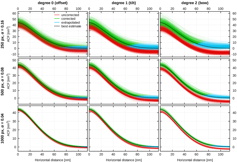
Figure 6: Autocorrelation functions obtained by model-free correction for rough SrO film surface, compared to uncorrected ACF and the best-estimate ACF. Each curve corresponds to one subimage cut from the large base image.

The large image was then cut to smaller images of various sizes and processed as above, assuming subimages are reasonable approximations of measurements on smaller areas. The uncorrected (red) and corrected (green) ACF computed for each subimage are plotted in figure 6 for three selected sizes and all three polynomial degree 0–2. The corrected ACF curves were extrapolated beyond the cut-off points by a simple subtraction of the last computed correction from all further data (cyan).

The correction is clearly effective. The green (corrected) curves, although spread slightly more than the red (uncorrected), are centred on the best estimate ACF. Deviations are noticeable only for the highest degree and the far ends of the curves, where there is a tendency to overcorrection.

5 Discussion

We first remark on the normalisation factor in (26) which is sometimes taken to be $1/N$ instead of $1/(N-k)$ because of positive definiteness and/or variance [7, 18, 19]. It corresponds to dividing the integrals in section 2 by $L$ instead of $L-\tau$. However, the estimator with $N-k$ denominator is unbiased, or at least it would be without background subtraction. Furthermore, a constant denominator $N$ does not generalise to irregular regions and other cases where varying amount of data is available for different distances $\tau$ [15]. Therefore, in this context $N-k$ is the appropriate choice.

5.1 Interpretation of results

Figure 6 almost looks too good to be true. One has to be careful with its interpretation. Everything was computed from the same large base image. The clustering of the green curves around the best estimate shows that we removed the bias tied to smaller scan areas. However, they do not necessarily cluster around the true ACF. In the example with synthetic Gaussian and pyramidal data, the surfaces were uniform and could be made infinite for all practical purposes. But for real rough surfaces, the issues of uniformity, representativeness and the statistical character of roughness are much more tangled. It should also be noted that roughness measurement is also affected by tip sharpness and probe-sample interaction in general [20, 21, 22, 23], sampling step [21, 24], calibration, scanning speed and feedback loop settings [22], defects, and other effects not analysed here as we attempt to isolate those related to the finite area.

The measurement of a neighbour region (somewhat smaller, $8\times 8\,\hbox{\textmu m}^{2}$) results in a slightly different ACF, as illustrated in figure 7. Subimages taken from this scan yield curves centred on its own best-estimate ACF. The bias estimates for the two images are approximately $3\times 10^{-4}$ and $6\times 10^{-4}$. The relative standard deviations of $G(0)=\sigma^{2}$ are proportional to $\alpha$ [8] were estimated as $2\times 10^{-3}$ and $3\times 10^{-3}$. They are all too small to explain the difference of almost 6 % between the two curves. The correlation length does not capture the scale at which real textures can be considered uniform. Although surface heights become uncorrelated for points considerably farther apart than $T$, the texture itself varies along the surface. The characteristic scale of these variations can be much longer than $T$ even if the texture is ultimately large-scale uniform. Scanning such large areas is seldom feasible and we have to rely on multiple independent scans.

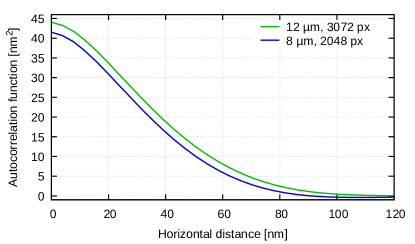
Figure 7: Comparison of best-estimate ACF obtained using independent scans of two different areas.

5.2 Comparison with spectral density

Two other functions are commonly used to characterise spatial properties of roughness, height-height correlation function [8] (sometimes also called structure function) and power spectrum density function (PSDF). Height-height correlation function $H$ is directly related to ACF by $H(\tau)+2G(\tau)=2\sigma^{2}$, so the results can be translated. PSDF is the Fourier transform of ACF and is probably the most commonly utilised function [21, 25]. The effect of levelling is suppression of low-frequency components [2].

The low-frequency components can be excluded from fitting, similarly how the ends of spectral range are avoided in PSDF stitching [26, 27, 18, 21, 28]. However, the peak around zero frequency is where almost all the spectral weight lies. It is also the least affected by noise, discontinuities and smoothing effects such as tip convolution [22, 21, 25]. It is often critical in roughness analysis. However, it is the region worst affected by levelling, and possibly in a non-trivial manner. In the case of ACF the worst affected region is far from the origin and it is never used for analysis. Around the origin, levelling manifests as the subtraction of a slowly varying function. An approach similar to the one developed here can perhaps be formulated also for PSDF—Ref. 1, for instance, gives hints at spectral reinterpretation. However, what would be the equivalent of model-free correction for PSDF is not clear.

5.3 Zero crossing

The model-free correction procedure relies on the true ACF monotonically and quickly decaying to zero. In particular, expressions (34) must give good approximations of integrals (30) (or similar integrals, but up to $L$ instead of infinity). Even though it is true for many types of real roughness, at least approximately, some violate this condition. For instance if the surface is locally periodic/corrugated the true ACF crosses zero, possibly many times. It may be possible to modify the correction procedure for this case, but likely at the cost of reliability. And although the approach of fitting $\hat{G}_{k}$ with biased model remains intact in principle, the first zero crossing may no longer be a good choice of fitting cut-off.

All the procedures utilise the zero crossing for choosing the cut-off in some manner. Must there always be a zero crossing? By splitting the sum $z_{m}z_{k}$ over all $m$ and $k$ into triangular parts and correcting for the double-counted diagonal

$$\sum_{m,k=0}^{N-1}z_{m}z_{k}=2\sum_{k=0}^{N-1}\sum_{m=0}^{N-1-k}z_{m+k}z_{k}-\sum_{k=0}^{N-1}z_{k}^{2}=2\sum_{k=0}^{N-1}(N-k)\hat{G}_{k}-N\hat{G}_{0}\;.$$ (38)

The left hand side is zero since the mean value of $z$ is zero. Therefore,

$$-\frac{N}{2}\hat{G}_{0}+\sum_{k=0}^{N-1}(N-k)\hat{G}_{k}=\frac{N}{2}\hat{G}_{0}+\sum_{k=1}^{N-1}(N-k)\hat{G}_{k}=0$$ (39)

and $\hat{G}_{k}$ must take both signs. As for the crossing location, the leading term approximation of the analytical models or (31) is a small constant (proportional to $M_{0}[G]$ or $S_{0}[G]$). If ACF decays quickly, the first zero crossing occurs when the true ACF is equal to this constant. And this is also when $S_{0}[G]$ and $S_{1}[G]$ can be assumed to give good approximations to the corresponding integrals.

For biased model fitting, the heuristic zero-crossing rule is further supported by the following:

• The rule is simple and easy to implement both manually and in code.

• Fitting only data of the ACF apex at origin is an ill-conditioned problem. The optimal bias–variance trade-off invariably includes the side slopes in the fit. Shortening the interval too much cannot be beneficial.

• Although fitting beyond the zero crossing may be beneficial, often the ACF is not converged in this region and telling where useful data end is difficult.

• Numerical simulations support the zero crossing as a good choice (section 4.2).

6 Conclusion

The goal of this work was to correct the finite-area bias in autocorrelation function (ACF) evaluation in roughness measurements, which includes the correction of parameters like the mean square roughness and correlation length. Starting from the observation that it should be possible to express the bias of measured ACF in terms of ACF itself, we developed a self-consistent formulation and used it to propose two types of bias correction. One was a modification of standard analytical ACF models to take into account the bias of the data they should fit. The other was a model-free correction procedure based on inverting the self-consistent relations by solving a set of linear equations. Their effectiveness was tested using simulated and measured data.

The two corrections behave similarly. They appear most helpful in the cases when they are also needed the most, that is the common moderate scan line lengths, as data for too short scan lines are not salvageable and for very long profiles the bias may already be small. Furthermore, they are more beneficial for higher levelling polynomial degrees for which the bias is worse. Both also trade bias for variance and thus the accuracy improvement is larger when multiple scans are evaluated. Modified (biased) analytical ACF models do not require any fundamental changes to the evaluation and can even be used to re-analyse existing raw ACF data. Based on numerical results, the measurement of Gaussian roughness, fitting the experimental ACF with a modified model has substantial advantages and few downsides and can probably be recommended quite universally. The model-free correction (inversion) procedure proposed for ACF of an unknown form is computationally efficient and worked surprisingly well in the selected test cases. A simple zero crossing based criterion was proposed for choosing the subset of discrete ACF data to use in the inversion. However, open question remains regarding the application of the procedure to ACFs of more complicated forms as the simple criterion may then no longer be suitable. The second correction method thus should be currently considered more an interesting concept to explore in further works.

Acknowledgements

I would like to thank my colleagues Marek Eliáš and Lenka Zajíčková for the rough samples used in the experimental part. This research was funded by Czech Science Foundation under project GACR 21-12132J. The CzechNanoLab project LM2023051 funded by MEYS CR is acknowledged for the financial support of the measurements and sample fabrication at CEITEC Nano Research Infrastructure.

References

References

- [1] Nečas D, Klapetek P and Valtr M 2020 Meas. Sci. Technol. 31 094010
- [2] Nečas D, Valtr M and Klapetek P 2020 Sci. Rep. 10 15294
- [3] Starink J P and Jovin T M 1996 Surface Science 359 291–305
- [4] Erickson B W, Coquoz S, Adams J D, Burns D J and Fantner G E 2012 Beilstein J. Nanotechnol. 3 747–758
- [5] Wang Y, Lu T, Li X and Wang H 2018 Beilstein J. Nanotechnol. 9 975–985 ISSN 2190-4286
- [6] Marinello F, Bariani P, Chiffre L D and Savio E 2007 Meas. Sci. Technol. 18 689
- [7] Anderson T W 1971 The Statistical Analysis of Time Series Wiley series in probability and mathematical statistics (New York: John Wiley & Sons)
- [8] Zhao Y, Wang G C and Lu T M 2000 Characterization of Amorphous and Crystalline Rough Surface – Principles and Applications (Experimental Methods in the Physical Sciences vol 37) (San Diego: Academic Press)
- [9] Krishnan V and Chandra K 2015 Probability and Random Processes 2nd ed (Wiley)
- [10] Hyndman R and Wand M 1997 Australian Journal of Statistics 39 313–324
- [11] Park C, Hannig J and Kang K H 2009 Statistica Sinica 19 1511–1530
- [12] Maxima 2023 Maxima, a computer algebra system. version 5.45.1 URL https://maxima.sourceforge.io/
- [13] Hestenes M R and Stiefel E 1952 J. Res. Nat. Bur. Stand. 49 409–436
- [14] Golub G H and Meurant G 2010 Matrices, Moments and Quadrature with Applications (New Jersey: Princeton University Press)
- [15] Nečas D and Klapetek P 2012 Cent. Eur. J. Phys. 10 181–188
- [16] Nečas D and Klapetek P 2021 Nanomaterials 11 1746
- [17] ISO 25178 2012 Geometric product specifications (GPS) – surface texture: Areal
- [18] Panda S, Panzade A, Sarangi M and Roy Chowdhury S K 2016 Journal of Tribology 139 031402
- [19] Bittani S 2019 Model Identification and Data Analysis (Agawam: Wiley)
- [20] Sedin D L and Rowlen K L 2001 Appl. Surf. Sci. 182 40–48 ISSN 0169-4332
- [21] Jacobs T D, Junge T and Pastewka L 2017 Surface Topography: Metrology and Properties 5 013001
- [22] González Martínez J F, Nieto-Carvajal I, Abad J and Jaime C 2012 Nano Express 7 174
- [23] Leach R, Weckenmann A, Coupland J and Hartmann W 2014 Surface Topography: Metrology and Properties 2 035001
- [24] Sanner A, Nöhring W G, Thimons L A, Jacobs T D and Pastewka L 2022 Applied Surface Science Advances 7 100190
- [25] Rutigliani V, Lorusso G F, Simone D D, Lazzarino F, Rispens G, Papavieros G, Gogolides E, Constantoudis V and Mack C A 2018 Setting up a proper power spectral density (PSD) and autocorrelation analysis for material and process characterization Metrology, Inspection, and Process Control for Microlithography XXXII (Proc. SPIE vol 10585) ed Ukraintsev V A and Adan O p 105851K
- [26] Duparre A, Ferre-Borrull J, Gliech S, Notni G, Steinert J and Bennett J 2002 Appl. Opt. 41 154–171
- [27] Gong Y, Misture S T, Gao P and Mellott N P 2016 The Journal of Physical Chemistry C 120 22358–22364
- [28] Klapetek P, Yacoot A, Grolich P, Valtr M and Nečas D 2017 Meas. Sci. Technol. 28 034015