Uncertainty Estimation of Transformers’ Predictions via Topological Analysis of the Attention Matrices

Abstract

Determining the degree of confidence of deep learning model in its prediction is an open problem in the field of natural language processing. Most of the classical methods for uncertainty estimation are quite weak for text classification models. We set the task of obtaining an uncertainty estimate for neural networks based on the Transformer architecture. A key feature of such mo-dels is the attention mechanism, which supports the information flow between the hidden representations of tokens in the neural network. We explore the formed relationships between internal representations using Topological Data Analysis methods and utilize them to predict model’s confidence. In this paper, we propose a method for uncertainty estimation based on the topological properties of the attention mechanism and compare it with classical methods. As a result, the proposed algorithm surpasses the existing methods in quality and opens up a new area of application of the attention mechanism, but requires the selection of topological features.

1 Introduction

In deep learning theory, Transformers are a class of neural networks for processing text data. During the training stage model recognizes grammatical and semantic relationships between words in a sentence through the interaction between their internal representations. The permanent exchange of information between token representations allows the model to determine which of the words are most important for understanding each other. This interaction is called the Attention mechanism and ensures high accuracy of Transformers predictions on the main types of NLP problems, including text classification.

However, for the practical use of neural networks, one should consider not only the percentage of correct predictions, but also the degree of confidence in each prediction. Transformers solving a text classification problem can produce unreliable answers. First, as typical classification models, they are poorly calibrated in probability  Guo et al. (2017). We expect that the incorrect predictions of the neural network correspond to a low (close to $0.5$) probability of the selected class. But classification models tend to overestimate their confidence in the prediction, resulting in a shift in probabilities closer to one. Secondly, Transformers suffer from adversarial attacks  Guo et al. (2021): a small perturbation in the input of the attacked model causes a significant change in its output. Therefore, it is crucial to have a mechanism to identify untrustworthy predictions in situations where model errors are unacceptable.

This issue is addressed to uncertainty estimation methods. The simplest way to get an uncertainty estimate for classification task is the output of the Softmax layer of the model, interpreted as a probability. More advanced approaches are Bayesian and ensemble methods, as well as MC dropout, which will be discussed in detail in the  2 Section. When applied to Transformers, these approaches have low computational efficiency or require significant modifications of the model setting.

The use of hidden representations of data has a potential to improve the quality of uncertainty estimates for Transformers. An effective method for detecting objects that such models regard as outliers uses the distances between the embeddings of the last layer  Vazhentsev et al. (2022). It is based on the fact that the neural network maps from the space of objects to the space of internal representations, in which the concept of distance can be defined. Objects from the same distribution correspond to closely spaced embeddings, while internal outlier representations are far away from them. This method is resource efficient, shows consistently high results in metrics, and points to the promise of using Transformers’ internal mechanism to estimate uncertainty.

In this paper, we develop the idea of determining the degree of model confidence in the prediction by its internal response to the input tokens. To characterize the structure of the Attention mechanism, we use its graph representation and apply methods of topological data analysis to it. Our main contributions are listed below:

• We obtain a complete description of the attention mechanism as a set of topological statistics. Topological features can characterize each attention matrix independently (feature type $1$) or pairs of attention matrices located in the different parts of the network (feature type $2$). While in earlier works  Cherniavskii et al. (2022),  Kushnareva et al. (2021) only features of type $1$ are considered, we are using features of type $2$ to analyze Transformers for the first time. We show that topological statistics help improve the estimate of model uncertainty.

• We propose an approximation of the model confidence by a trainable analog of the probability for each prediction. We introduce suitable training pipeline and loss function for connecting topological statistics with uncertainty of predictions.

• Our confidence prediction algorithm outperforms baseline methods on three models determining grammatical correctness of sentences in English, Russian and Italian, respectively.

2 Related work

There are several ways to estimate uncertainty for deep neural networks. For classification models one can utilize the output of the Softmax layer, interpreted as a class probability. The authors of  Geifman and El-Yaniv (2017) propose a Softmax Response method based on the maximum probability $p(y|x)$ of belonging to the class $y=c\in C$ at the model output. The higher this probability, the more confident the model is in the prediction:

$$u_{SR}(x)=1-\max_{c\in C}p(y=c|x)$$ (1)

The main advantage of this approach is that it does not require additional calculations: the required estimate is obtained automatically at the output of the last layer of the model. However, Softmax probabilities are not really credible, as models tend to be overconfident  Guo et al. (2017).

The classical method for uncertainty estimation, which has a fundamental theoretical proof, is the Bayesian approach  Blundell et al. (2015). It initially sets a prior distribution on the model parameters, and then, based on the training samples, calculates the posterior distribution on the weights. In order to apply the Bayesian approach in practice, various approximations are used  Van Amersfoort et al. (2020) and the choice of approximation greatly affects the quality of the estimate. In general, Bayesian neural networks capable of obtaining reliable estimates of uncertainty require significant changes in the training scheme and learn more slowly than classical neural networks.

For classical neural networks, there is another way to introduce variability into the model parameters without changing the architecture and learning process  Lakshminarayanan et al. (2017). It is based on training deep ensembles: several copies of the original model are trained independently and after that predictions of the resulting uncorrelated models are averaged. However, the quality of the uncertainty estimate increases with the number of models in the ensemble, and, accordingly, with the computational cost of their training.

The ideas of the previous two methods are developed by the more resource-efficient Monte Carlo (MC) Dropout method  Gal and Ghahramani (2016). It interprets the dropout layer, widely known regularization technique in deep neural networks, as a Bayesian approximation of a probabilistic model: a Gaussian process. Neural networks with different sets of deactivated neurons can be considered as Monte Carlo samples from the space of all possible neural networks. So, the same uncertainty estimation methods work for them as for ensembles. It is important that dropout must be enabled at the testing stage for the diversity of the predictions, as opposed to the classical use of the layer at the training stage. The main advantage of this approach is that single trained model is enough to estimate the uncertainty, while the disadvantage is the amount of computation for neural network runs with different sets of disabled neurons. Other approaches that can provide uncertainty estimation for deep neural networks train a separate head for this goal Kendall and Gal (2017); Kail et al. (2022). While these approaches often focuses on computer vision, they can be adopted as well in the natural language processing.

There are also methods for uncertainty estimation which use the Mahalanobis distance - a generalization of the Euclidean distance for vectors of random variables - between the internal representations of the training and test objects. The article  Lee et al. (2018) explores the use of the Mahalanobis distance between the test samples and the nearest class conditional Gaussian distribution as an uncertainty estimate:

$$u_{md}=\min_{c\in C}(h_{i}-\mu_{c})^{T}\Sigma^{-1}(h_{i}-\mu_{c})$$ (2)

where $h_{i}$ is the hidden representation of the test sample, $\mu_{c}$ is the centroid of the $C$ class, $\Sigma$ is the covariance matrix of the hidden representations of the training samples. An advantage of this method is that it does not require significant changes in the architecture of the model and the memory and time costs of training and storing multiple copies of the model. Obtaining an uncertainty estimate only adds a small amount of computation to the model testing phase. A disadvantage of this approach is the need to obtain internal representations for the whole training examples, which may take more time than several forward passes of the neural network on the test dataset for MC dropout evaluation. This is due to the fact that the training dataset is much larger than the test dataset.

As a result, each of the existing methods for uncertainty estimation of neural network predictions has its own benefits and limitations, which, in turn, strongly depend on the task, the amount of available resources and the required quality of the estimate. In terms of the ratio of computational efficiency and reliability of the obtained estimate, the MC dropout methods and the Mahalanobis distance between internal representations are leading. However, most comparisons of methods for uncertainty estimation in the literature are carried out for computer vision problems and their effectiveness for problems of natural analysis is still unclear. Also, in works where uncertainty is evaluated for Transformers  Shelmanov et al. (2021),  Vazhentsev et al. (2022), the approaches and modifications proposed to them only occasionally consider the key feature of the architecture, namely the Attention mechanism. The proposed algorithm for calibrating neural model predictions by the degree of confidence not only produces high-quality estimates specifically for the NLP task, but also opens up another potential area of application of the attention mechanism - uncertainty estimation.

3 Problem Statement

3.1 Confidence Score

We formalize the problem of estimating uncertainty for a pretrained Transformer model with fixed weights. For each sample $x$, we need to get the Confidence Score $c(x)\in[0,1]$ expressing the degree of confidence of the neural network in the prediction $f_{\theta}(\bf{x})$. The task of uncertainty estimation in our case is to find the function $c(Attention(x))$.

3.2 Testing Method

The search for a suitable metric for our problem is complicated due to the fact that uncertainty estimation belongs to the class of unsupervised problems. There are no targets for a measure of the model’s confidence in its prediction in the training dataset.

In order to correctly evaluate the estimate of model uncertainty, we focus on the correlation between the confidence of the model and the accuracy of its predictions. We use the following test pipeline:

• For each of the $N$ test samples, we get the prediction of the neural network and the Confidence Score.

• We rank objects by Confidence Score in ascending order: from less confident objects to more confident ones. We calculate and save the accuracy score on the whole test dataset.

• We iteratively remove the $r$ least confident samples and calculate the metric on $N-ir$ remaining samples, where $i$ is the iteration number.

• On the graph, we display the dependence of the accuracy score for the remaining subset on the portion of removed objects $\frac{ir}{N}$

The graph of the obtained dependence is called Accuracy Rejection Curve  Nadeem et al. (2009) and the area under the graph is used as the numerical value of the metric. It is common to calculate the area from the accuracy level for the whole test dataset, not taking into account the rectangular area below this level.

The plot of the Accuracy Rejection curve can be interpreted as follows: a model correctly calibrated for uncertainty makes errors mainly on examples with a low Confidence Score. The graph shows that after removing a small number of such uncertain examples, the accuracy of predictions on the remaining subset increases significantly. In practice, one can ask experts to make predictions on these examples instead of a neural network, and thus the probability of error for a hybrid system from a model and experts will be minimized. The most effective method for assessing uncertainty in this case minimizes the number of examples that must be given to experts for analysis.

4 Method Description

In this section, we consider in more detail topological statistics of the Attention mechanism and propose a training scheme for our method.

4.1 Topological analysis of the Attention mechanism

Attention matrix has an equivalent representation in the form of a weighted directed graph $G$. The vertices of such a graph are the tokens of the input sequence, and the weights of the edges are the attention weights for each pair of tokens. The direction of the edge is chosen from the request token to the key token. Using this method, for each input sentence, we get $N_{l}*N_{h}$ attention graphs, where $N_{l}$ is the number of layers, $N_{h}$ is the number of Transformer heads.

Our task is to extract from graph representations a set of numerical statistics for each sentence  Kushnareva et al. (2021). First, we calculate graph features: the number of vertices, edges, connected components, simple cycles, and Betti numbers. This set of statistics is not exhaustive, as it does not involve edge weights. The way to take into account the presence of weights is to construct a filtration - a family of graphs $\{G^{t_{i}}\}$ obtained from the original one by removing edges with a weight less than the threshold $t_{i}$  barcode. Successive reduction of edges leads to a change in the structure of the graph and its main properties listed above. The methods of topological data analysis make it possible to quantitatively describe the evolution of graph properties by determining for each property the time of its appearance and disappearance in the filtration (the corresponding thresholds are denoted by $t_{birth}$ and $t_{death}$). The set of intervals between $t_{birth}$ and $t_{death}$ is called a barcode and is a measure of the stability of the attention structure of  Cherniavskii et al. (2022) graphs. The most stable and pronounced graph properties will have the largest barcode length. We extract the following numerical statistics from barcodes: sum, mean, variance and entropy of barcode lengths, number of barcodes with appearance/disappearance times less/greater than the threshold value.

An analysis of attention graphs  Kovaleva et al. (2019) taken from different heads and layers of the network shows that in the process of filtering graphs have similar structural elements/patterns. In the article Clark et al. (2019) these patterns are divided into several main types: attention to the current, previous and next tokens, attention to service [SEP] and [CLS] tokens. The authors Kushnareva et al. (2021) propose a graph representation method for attention patterns and introduce template features based on it. Numerically, it is equal to the Frobenius norm of the difference between the attention matrix and the incidence matrix of the attention pattern.

The topological features listed above are calculated independently for attention graphs from different layers and heads of the network, however, the attention mechanisms in different parts of the model are trained jointly and it is better to take into account the connection between them. The cross-barcode method Barannikov et al. (2021) develops the idea of barcodes and allows to compare the distributions of attention weights on different layers and heads of the neural network. Consider two attention graphs $G^{w}$ and $G^{w^{\prime}}$, where $w$ and $w^{\prime}$ are attention weights, as well as a matrix composed of pairwise minimum of the weights $M=min(w,w^{\prime})$ and the corresponding graph $G^{min(w,w^{\prime})}$. The main difference from barcodes is that the filtering is performed for the graph $G^{w,w^{\prime}}$ constructed from $G^{w}$ and $G^{min(w,w^{\prime})}$. After filtering, we get a set of intervals $(t_{birth},t_{death})$ and calculate the value of the topological feature as the total length of the cross-barcode segments. Intuitively, the cross-barcode expresses simpler graph properties (the number of simple cycles, connected components, etc.), which, at a fixed $\alpha$ threshold, have already appeared/disappeared in one of the graphs, but have not yet appeared/disappeared in another graph .

Using the methods above, from the graph representation of the attention matrices for each input sentence, we obtain a set of topological features of 4 types:

• graph statistics (graph features)

• features obtained from barcodes
  (barcode/ripser features)

• features obtained from attention patterns
  (template features)

• features obtained from cross-barcodes
  (cross-barcode features)

The first 3 types of features are calculated for attention matrices independently and belong to the first type, the last type of features is calculated for pairs of matrices and belongs to the second type.

The linguistic interpretation of features is that graph structures are used in lexicology to describe the laws of semantic changes in a language Hamilton et al. (2016). The evolution of the meaning of a word over time can be represented as a graph in which the edges are proportional to the semantic shift relative to different meanings of the word. A similar evolutionary process occurs within a neural model as the hidden representation of a word changes from the initial layers of the network to deeper layers. Groups of tokens with strong mutual influence form separate clusters in a graph representation, just as words related in meaning and syntactically in a sentence form phrases. Barcodes highlight the dominant, most stable semantic relationships between words, and attention patterns highlight the main directions of interaction between context tokens.

4.2 Confidence predictor model and its training

Formally, given the input set of features $(z_{1},z_{2},\cdots z_{n})$, the algorithm should produce the number Confidence Score $c\in[0,1]$. This range of values allows us to interpret the Confidence Score as a probability, thus the problem of estimating the confidence of the Transformer in the prediction is reduced to a standard binary classification problem. We use a separate Score Predictor model for it, consisting of several fully connected layers and activation functions between them. The last activation function should be sigmoid to limit the output of the model to $[0,1]$. The simplicity of the architecture is explained by the high risk of overfitting. We get an increase in the predictive ability of the model by more careful selection and aggregation of topological features instead of making the network deeper.

The key point is to build the loss function for our model. Cross-entropy, which is widely used by models for binary classification, does not suit us, since the target distribution of the Confidence Score is not available. Also, optimizing the loss function should reward the neural network for obtaining uncertainty estimates that truly reflect Transformer’s ability to predict the correct class for any input. Similar to the method proposed in  DeVries and Taylor (2018), we choose the cross-entropy modification as the loss function, in which the probability at the output of the model is calibrated using the Confidence Score.

Let embeddings of words in a sentence $(x_{1},x_{2},\cdots x_{n})$, the corresponding set of topological features $(z_{1},z_{2},\cdots z_{m})$, Transformer output $\mathbf{p}=\mathrm{Softmax}(f(\mathbf{x},\mathbf{\theta}))$ and the uncertainty estimate for this prediction obtained from the Score Predictor model $c=\mathrm{Sigmoid}(g(\mathbf{z},\mathbf{w}))$, while $p_{1},p_{2},c\in[0,1],p_{1}+p_{2}=1$. Then the calibrated probability is obtained by interpolating between the Transformer’s prediction and its one-hot target distribution $\mathbf{y}$ with the degree of interpolation determined by the Confidence Score: $p^{\prime}_{i}=cp_{i}+(1-c)y_{i}$. The final loss function

$$L=-\sum_{i=1}^{2}\log(p^{\prime}_{i})y_{i}-\lambda\log(c)$$ (3)

is the sum of cross-entropy with calibrated probability and regularization, which penalizes the model for uncertain predictions. The ratio of the main loss and regularization is determined by the $\lambda$ hyperparameter.

Let’s analyze how Confidence Score affects the dynamics of the loss function. For $c\rightarrow 1$ (case of sure prediction) $p\rightarrow p^{{}^{\prime}}$ and the value of the loss is determined by the original Transformer prediction without any uncertainty estimate. On the contrary, for $c\rightarrow 0$, instead of an uncertain prediction, the loss function receives the target distribution, preventing the error from growing. If $c$ is between 0 and 1, then the calibrated probability becomes closer to the target penalty cost in the regularization term. In general, a decrease in the loss function corresponds to an increase in the Confidence Score on correct predictions and a decrease in it on erroneous predictions, which is what we need. It is also important that all transformations in the error functional are differentiable, but only the parameters of the Score Predictor model are trained. Any change in the weights of the Transformer will lead to a change in the topology of the attention mechanism and will require recalculation of topological features, so the weights of the Transformer are fixed in the process of estimating the uncertainty.

5 Experiments

This section provides implementation details of our uncertainty estimation algorithm, data and model details, and experimental results.

5.1 Data

We are experimenting on 3 Corpus of Linguistic Acceptability (CoLA)  Warstadt et al. (2019) datasets, consisting of sentences in English, Italian and Russian. Each sentence has a target value: 1 for grammatically correct sentences, 0 otherwise. Basic information about datasets is given in the Appendix A.

5.2 Models

The standard approach to using BERT-like models is to finetune the pre-trained models  Devlin et al. (2019) that are publicly available. Pre-trained neural networks have sufficient generalization ability to condition on a specific task in just a few epochs of retraining with a low learning rate.

In this work, we use pre-trained BERT-base-cased models from the Transformers library. Hyperparameters of finetuning and final model metrics are given in the Appendix A.

5.3 Basic Methods

We compare the results of our algorithm with three classical methods of uncertainty estimation: Softmax Response, MC Dropout, Mahalanobis estimator. The implementation of the last two methods was based on the code for the article  Vazhentsev et al. (2022). Also, we checked the strategy of training the Score Predictor on the BERT embeddings extracted from its classification part instead of topological statistics. This approach is successfully used in the article  DeVries and Taylor (2018) for computer vision tasks, however, the decrease in the performance of this method for NLP tasks provides motivation for applying TDA methods instead.

5.4 Extraction of topological features

Each of the BERT-like neural networks considered in this paper contains 12 layers and 12 heads on each layer, respectively, for each input object, we extract 144 attention matrices. Then, for each matrix, we extract 3 types of type 1 topological features, discussed in detail in the 4.1 section: graph features, barcode features, template features. We calculate features of type 2 between pairs of attention matrices $A_{ik}$ and $A_{kj}$, where the first index corresponds to the layer number, the second index is the head number, $i,j,k\in\{0,12\}$. An example of a barcode for a test sample object is shown in the Appendix D. Barcodes are calculated using the Ripser++ Zhang et al. (2020) library, and cross-barcodes are calculated using the MTopDiv Barannikov et al. (2021) library. The algorithms implemented in these libraries use advanced optimizations, which can significantly reduce the time for computing topological features. As a result, for each input feature we get vectors of dimension (12, 12, 7) graph features, (12, 12, 14) barcode features, (12, 12, 5) template features, (12, 12, 144) cross-barcode features. The first dimension corresponds to the layer number, the second - to the head number, the third - to the subtype of the topological feature. All subtypes of topological features are listed in the Appendix C. To train the Score Predictor model, the selected feature vectors are concatenated along the third dimension.

5.5 Training setup of the Score Predictor

The model that predicts the Confidence Score takes a set of topological statistics as input and converts it into a scalar value of the uncertainty score as an output. It is training by minimizing the Confidence Loss introduced in the 4.2 section, so outputs of the Transformer Softmax layer and the distribution of target values for the original classification task are also given to the model as input. High quality estimates were obtained by Score Predictor model containing 2 fully connected layers with sigmoids as activation functions. Our optimal setup also includes the Adam optimization method and the training hyperparameters listed in the Appendix E.

5.6 Analysis of topological features of the first type

Let us consider separately the topological features of the first type. The total number of components in the vectors of topological features of 3 types for one object is $12*12*(7+14+5)=$3744. Considering that the number of objects in the training samples does not exceed 10000, the use of 3744 embeddings would guarantee overfitting. So it was necessary to reduce the number of components in the feature vector, and we considered two methods:

• averaging over all layers and all heads of the Transformer

• selection of the components that contribute most to the prediction using Shapley values Lundberg and Lee (2017)

Feature aggregation method	En-CoLA	Ita-CoLA	Ru-CoLA
averaging over all heads and layers	0.079	0.088	0.075
selection via Shapley values	0.087	0.093	0.080

Table 1: Area under Accuracy Rejection curves for different methods of aggregation of topological features

The results of training the Score Predictor model only on the first type of topological features are given in the Table 1.

For each model, selection of the most significant components improved the uncertainty estimate in relation to simple averaging. Therefore, in further experiments, we feed the Score Predictor model with two components of topological features of the first type that most affect the result. Feature selection process via Shapley values is considered in detail in Appendix B.

5.7 Analysis of topological features of the second type

Since we found out earlier that the last layer attentions are the most informative for us, we also calculate cross-barcodes along this layer. We fix the index $k$ equal to 12, vary the indices $i$, $j$ and observe how the quality of the uncertainty estimation changes, when the Score Predictor receives the pairwise attention statistics of the matrices $Aik$ and $Akj$.

Table 2 shows the change in the metric when adding cross-barcodes to the English-language setup. According to the experimental results, there is a small portion of the optimal pairs of attention matrices. Cross-barcode calculated for such pair improves the uncertainty estimate for our topological method, for example, the pair $A_{12,12}$ and $A_{12,9}$. These pairs are located in the lower right corner of the table, which corresponds to the 7-12 layer and head indices in the Transformer. The remaining pairs of attention matrices barely improve the performance of Score Predictor.

	(12, 1)	(12, 3)	(12, 5)	(12, 7)	(12, 9)	(12, 11)
(2, 12)	0.085	0.085	0.085	0.086	0.086	0.086
(4, 12)	0.086	0.089	0.085	0.087	0.088	0.085
(6, 12)	0.086	0.087	0.087	0.086	0.087	0.088
(8, 12)	0.086	0.087	0.085	0.086	0.088	0.091
(10, 12)	0.085	0.086	0.087	0.086	0.087	0.086
(12, 12)	0.088	0.086	0.085	0.090	0.096	0.094

Table 2: Area under Accuracy Rejection curves for the topological method with the addition of cross-barcodes between the $A_{ik}$ and $A_{kj}$ matrices. The indices $(i,k)$ attention of the matrix $A_{ik}$ are placed vertically, the indices $(k,j)$ attention of the matrix $A_{kj}$ are placed horizontally

As a result, we supplement the set of topological features of the first type with the two most informative cross-barcodes. Further, our final results are given for the Score Predictor, trained only on best-performing topological features of each type.

6 Results

The area under the Accuracy Rejection curve for each method is presented in the Table  3. This metric has a theoretical upper bound, which depends on the accuracy of Transformer’s predictions on the full dataset. It can be interpreted as confidence of an Oracle, for which the condition $\forall x,x^{\prime}\rightarrow C(x)>C(x^{\prime})$ is satisfied, where $x$ is a correctly recognized object, $x^{\prime}$ is an incorrectly recognized object , $C(x)$ and $C(x^{\prime})$ are the corresponding Confidence Score values. Consequently, the plot of the Accuracy Rejection curve for an Oracle increases linearly while only incorrectly classified objects are disappearing from the subset, and then reaches a constant value of $1$.

Method type	Method name	En-CoLA	Ita-CoLA	Ru-CoLA
Basic Methods	Softmax Response	0.068	0.085	0.073
	MC Dropout 1	0.071	0.084	0.076
	Mahalanobis estimator 2	0.083	0.091	0.080
	Embedding estimator 3	0.075	0.090	0.074
Our methods	Topological estimator without cross-barcodes	0.087	0.092	0.080
	Topological estimator with cross-barcodes	0.098	0.099	0.085
Oracle Upper Bound		0.124	0.121	0.118

Table 3: Area under Accuracy Rejection curves for the considered methods

For all benchmarks we have considered, topological methods outperforms basic methods, and the addition of cross-barcode statistics leads to a significant increase in metric. This effect is most pronounced for the English-language BERT and leads to increase of 12 percent relative to the method using only topological statistics of first type, and the least pronounced for the Russian-language BERT, where the increase is 2 times less. Among the baselines, Softmax Response and MC Dropout show poor quality of uncertainty estimates, while Mahalanobis estimator gives a consistently reliable estimate and is practically comparable to our topological method without cross-barcodes. The results of the Embedding estimator method are not stable: for the Transformer working with Italian texts, they are close to the topological method without cross-barcodes, but for other models the Embedding estimator is inferior to the topological methods.

We highlight the key features of compared methods on the example of English-language benchmark. The graph 1 shows the Accuracy Rejection curves for the two basic methods, the Oracle upper estimate and our topological method using cross-barcodes. Firstly, the Accuracy Rejection curve for our method lies above the corresponding curves of the base methods and reaches a constant value earlier. Secondly, the main interest in practice is the initial part of the curve with rejection rate in $[0,0.2]$. For the topological method, this section is convex, while for the basic methods, the character of the initial sections is closer to linear. In practical application, convexity is preferable, since it means a noticeable increase in metric when only a small number of objects are removed.

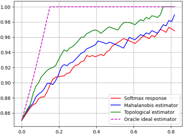
Figure 1: Accuracy rejection curves of the selected methods for the BERT-base model on the En-CoLA test set

7 Conclusion

Existing studies in the intersection of TDA and NLP domains prove that use of topological features of attention maps can boost classification performance. We show that topological statistics also allow to obtain an uncertainty estimates of Transformer predictions, and the quality of the estimates is superior to that of baselines. We prove this by experiments on three BERT models to determine the linguistic acceptability of sentences in English, Russian and Italian, respectively. The confidence prediction by topological method demonstrates an increase compared to the best of the basic methods up to 16 percent in metric.

Our algorithm for determining the confidence of the Transformer in its prediction uses two main types of topological statistics: features calculated for each attention matrix independently and pairwise statistics. The use of features of the second type for attention mechanism is our innovation and cross-barcodes significantly boost the quality of uncertainty estimation by proposed methods.

We found out that the location of the attention matrix in the Transformer affects the contribution of topological statistics. On average, the last layer features are the most informative, however, to achieve the highest possible quality of the estimate, careful selection of features is required. For topological features calculated independently, this process can be automated by selecting components with highest Shapley values.

Limitations

Our method also has some limitations: 1) Feature extraction slows down the inference (on average 20 sec per sample is required for feature computation with GPU acceleration). 2) Selection of the most informative attention matrices should be fully automatized. Calculation of topological statistics of both types only on a limited small set of attention matrices will significantly speed up our method and, quite likely, not reduce the quality of the uncertainty estimation. Optimization of mentioned calculations will be our main direction for further work in this area.

Appendix A Datasets and pretrained models info

Size of training and test sets for each benchmark is given in Table 4. Finetuning setups for BERT-base-cased models and final metrics are presented in the Table 5.

Appendix B Shapley values

Shapley values were introduced in game theory to distribute the payoff fairly among the players in a team according to the contribution of each of them to the result. In our case, the individual components of the vectors act as players, and the Shapley values express the influence of each component on the prediction. To calculate these values, we use the SHAP library. An example of the analysis of one subtypes of a graph feature (number of vertices) is shown in the graph 2 The largest variance of Shapley values corresponds to the greatest influence of the component on the prediction. According to the graph, the components from the last layer of the Transformer turned out to be the most important, since their indices are in the range of 130-144. Probably, the reason for the significance of the components from the last layer are caused by BERT finetuning. This process only affects the weights of the last layer, so they probably catches more specific properties of data than initial layers.

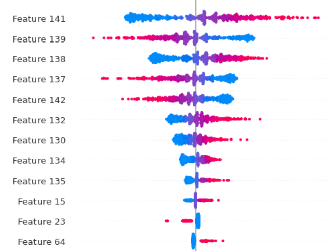
Figure 2: Analysis of graph feature components using Shapley values. The number of the component is plotted along the vertical axis, and the Shapley values along the horizontal axis. The color gradient from blue to pink corresponds to the increase in the absolute value of the graph feature

Dataset	Training set size	Test set size
En-CoLA	8551	527
Ita-CoLA	7801	946
Ru-CoLA	7869	984

Table 4: Number of sentences in datasets

Model	Dataset	Epochs	Batch size	Learning rate	Accuracy
BERT-base	En-CoLA	3	32	3e-5	0.850
	Ita-CoLA	3	64	3e-5	0.866
RuBERT	Ru-CoLA	3	32	3e-5	0.802

Table 5: Model configuration and final metrics on the test set

Appendix C Feature sybtypes

1. Graph statistics:

   • Number of vertices

   • Number of simple loops

   • Number of connectivity components

   • Number of edges

   • Average vertex degree

   • Betti numbers

2. Features received from barcodes:

   • Sum of barcode lengths

   • Variance of barcode lengths

   • Entropy of barcode lengths

   • Birth time of the longest barcode

   • Number of barcodes along the homology dimension

   • Number of barcodes with birth/death times greater than/less than a fixed threshold

3. Features obtained from attention patterns:

   • Distance to previous token

   • Distance to current token

   • Distance to next token

   • Distance to classification token

   • Distance to punctuation marks

4. Features obtained from cross-barcodes:

   • Sum of lengths of cross-barcode segments

Appendix D Cross-barcode sample

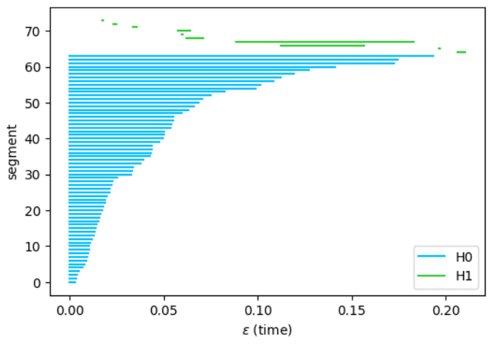
Figure 3: An example of a cross-barcode between pairs of Attention matrices, given by the numbers of the layer and the head of the Transformer (6, 11) and (11, 6). H0 and H1 correspond to 0- and 1-dimensional homology

Appendix E Training configuration of Score Predictor

By grid search we selected the optimal set of training hyperparameters:

N epochs = 250, learning rate = $1e^{-3}$, $\lambda=0.01$

References

- Barannikov et al. (2021) Serguei Barannikov, Ilya Trofimov, Grigorii Sotnikov, Ekaterina Trimbach, Alexander Korotin, Alexander Filippov, and Evgeny Burnaev. 2021. Manifold topology divergence: a framework for comparing data manifolds. In Advances in Neural Information Processing Systems, volume 34, pages 7294–7305. Curran Associates, Inc.
- Blundell et al. (2015) Charles Blundell, Julien Cornebise, Koray Kavukcuoglu, and Daan Wierstra. 2015. Weight uncertainty in neural network. In Proceedings of the 32nd International Conference on Machine Learning, volume 37, pages 1613–1622. PMLR.
- Cherniavskii et al. (2022) Daniil Cherniavskii, Eduard Tulchinskii, Vladislav Mikhailov, Irina Proskurina, Laida Kushnareva, Ekaterina Artemova, Serguei Barannikov, Irina Piontkovskaya, Dmitri Piontkovski, and Evgeny Burnaev. 2022. Acceptability judgements via examining the topology of attention maps. In Findings of the Association for Computational Linguistics: EMNLP 2022, pages 88–107, Abu Dhabi, United Arab Emirates. Association for Computational Linguistics.
- Clark et al. (2019) Kevin Clark, Urvashi Khandelwal, Omer Levy, and Christopher D. Manning. 2019. What does BERT look at? an analysis of BERT’s attention. In Proceedings of the 2019 ACL Workshop BlackboxNLP: Analyzing and Interpreting Neural Networks for NLP, pages 276–286, Florence, Italy. Association for Computational Linguistics.
- Devlin et al. (2019) Jacob Devlin, Ming-Wei Chang, Kenton Lee, and Kristina Toutanova. 2019. BERT: Pre-training of deep bidirectional transformers for language understanding. In Proceedings of the 2019 Conference of the North American Chapter of the Association for Computational Linguistics: Human Language Technologies, Volume 1 (Long and Short Papers), pages 4171–4186, Minneapolis, Minnesota. Association for Computational Linguistics.
- DeVries and Taylor (2018) Terrance DeVries and Graham W. Taylor. 2018. Learning confidence for out-of-distribution detection in neural networks. ArXiv, abs/1802.04865.
- Gal and Ghahramani (2016) Yarin Gal and Zoubin Ghahramani. 2016. Dropout as a bayesian approximation: Representing model uncertainty in deep learning. In Proceedings of The 33rd International Conference on Machine Learning, volume 48 of Proceedings of Machine Learning Research, pages 1050–1059. PMLR.
- Geifman and El-Yaniv (2017) Yonatan Geifman and Ran El-Yaniv. 2017. Selective classification for deep neural networks. In Advances in Neural Information Processing Systems, volume 30. Curran Associates, Inc.
- Guo et al. (2017) Chuan Guo, Geoff Pleiss, Yu Sun, and Kilian Q. Weinberger. 2017. On calibration of modern neural network. In Proceedings of the 34th International Conference on Machine Learning, volume 70, pages 1321–1330.
- Guo et al. (2021) Chuan Guo, Alexandre Sablayrolles, Hervé Jégou, and Douwe Kiela. 2021. Gradient-based adversarial attacks against text transformers. In Proceedings of the 2021 Conference on Empirical Methods in Natural Language Processing, pages 5747–5757, Online and Punta Cana, Dominican Republic. Association for Computational Linguistics.
- Hamilton et al. (2016) William L. Hamilton, Jure Leskovec, and Dan Jurafsky. 2016. Diachronic word embeddings reveal statistical laws of semantic change. In Proceedings of the 54th Annual Meeting of the Association for Computational Linguistics (Volume 1: Long Papers), pages 1489–1501, Berlin, Germany. Association for Computational Linguistics.
- Kail et al. (2022) Roman Kail, Kirill Fedyanin, Nikita Muravev, Alexey Zaytsev, and Maxim Panov. 2022. Scaleface: Uncertainty-aware deep metric learning. arXiv preprint arXiv:2209.01880.
- Kendall and Gal (2017) Alex Kendall and Yarin Gal. 2017. What uncertainties do we need in bayesian deep learning for computer vision? Advances in neural information processing systems, 30.
- Kovaleva et al. (2019) Olga Kovaleva, Alexey Romanov, Anna Rogers, and Anna Rumshisky. 2019. Revealing the dark secrets of BERT. In Proceedings of the 2019 Conference on Empirical Methods in Natural Language Processing and the 9th International Joint Conference on Natural Language Processing (EMNLP-IJCNLP), pages 4365–4374, Hong Kong, China. Association for Computational Linguistics.
- Kushnareva et al. (2021) Laida Kushnareva, Daniil Cherniavskii, Vladislav Mikhailov, Ekaterina Artemova, Serguei Barannikov, Alexander Bernstein, Irina Piontkovskaya, Dmitri Piontkovski, and Evgeny Burnaev. 2021. Artificial text detection via examining the topology of attention maps. In Proceedings of the 2021 Conference on Empirical Methods in Natural Language Processing, pages 635–649, Online and Punta Cana, Dominican Republic. Association for Computational Linguistics.
- Lakshminarayanan et al. (2017) Balaji Lakshminarayanan, Alexander Pritzel, and Charles Blundell. 2017. Simple and scalable predictive uncertainty estimation using deep ensembles. In Advances in Neural Information Processing Systems, volume 30. Curran Associates, Inc.
- Lee et al. (2018) Kimin Lee, Kibok Lee, Honglak Lee, and Jinwoo Shin. 2018. A simple unified framework for detecting out-of-distribution samples and adversarial attacks. In Advances in Neural Information Processing Systems, volume 31. Curran Associates, Inc.
- Lundberg and Lee (2017) Scott M Lundberg and Su-In Lee. 2017. A unified approach to interpreting model predictions. In Advances in Neural Information Processing Systems, volume 30. Curran Associates, Inc.
- Nadeem et al. (2009) Malik Sajjad Ahmed Nadeem, Jean-Daniel Zucker, and Blaise Hanczar. 2009. Accuracy-rejection curves (arcs) for comparing classification methods with a reject option. In International Workshop on Machine Learning in Systems Biology.
- Shelmanov et al. (2021) Artem Shelmanov, Evgenii Tsymbalov, Dmitri Puzyrev, Kirill Fedyanin, Alexander Panchenko, and Maxim Panov. 2021. How certain is your Transformer? In Proceedings of the 16th Conference of the European Chapter of the Association for Computational Linguistics: Main Volume, pages 1833–1840, Online. Association for Computational Linguistics.
- Van Amersfoort et al. (2020) Joost Van Amersfoort, Lewis Smith, Yee Whye Teh, and Yarin Gal. 2020. Uncertainty estimation using a single deep deterministic neural network. In Proceedings of the 37th International Conference on Machine Learning, volume 119, pages 9690–9700. PMLR.
- Vazhentsev et al. (2022) Artem Vazhentsev, Gleb Kuzmin, Artem Shelmanov, Akim Tsvigun, Evgenii Tsymbalov, Kirill Fedyanin, Maxim Panov, Alexander Panchenko, Gleb Gusev, Mikhail Burtsev, Manvel Avetisian, and Leonid Zhukov. 2022. Uncertainty estimation of transformer predictions for misclassification detection. In Proceedings of the 60th Annual Meeting of the Association for Computational Linguistics (Volume 1: Long Papers), pages 8237–8252, Dublin, Ireland. Association for Computational Linguistics.
- Warstadt et al. (2019) Alex Warstadt, Amanpreet Singh, and Samuel Bowman. 2019. Neural network acceptability judgments. Transactions of the Association for Computational Linguistics, 7.
- Zhang et al. (2020) Simon Zhang, Mengbai Xiao, and Hao Wang. 2020. Gpu-accelerated computation of vietoris-rips persistence barcodes. In 36th International Symposium on Computational Geometry (SoCG 2020). Schloss Dagstuhl-Leibniz-Zentrum für Informatik.