The modified Yule-Walker method for multidimensional infinite-variance periodic autoregressive model of order 1

Abstract

The time series with periodic behavior, such as the periodic autoregressive (PAR) models belonging to the class of the periodically correlated processes, are present in various real applications. In the literature, such processes were considered in different directions, especially with the Gaussian-distributed noise. However, in most of the applications, the assumption of the finite-variance distribution seems to be too simplified. Thus, one can consider the extensions of the classical PAR model where the non-Gaussian distribution is applied. In particular, the Gaussian distribution can be replaced by the infinite-variance distribution, e.g. by the $\alpha-$stable distribution. In this paper, we focus on the multidimensional $\alpha-$stable PAR time series models. For such models, we propose a new estimation method based on the Yule-Walker equations. However, since for the infinite-variance case the covariance does not exist, thus it is replaced by another measure, namely the covariation. In this paper we propose to apply two estimators of the covariation measure. The first one is based on moment representation (moment-based) while the second one - on the spectral measure representation (spectral-based). The validity of the new approaches are verified using the Monte Carlo simulations in different contexts, including the sample size and the index of stability of the noise. Moreover, we compare the moment-based covariation-based method with spectral-based covariation-based technique. Finally, the real data analysis is presented.

1 Introduction

In many real applications, one can observe the periodic behavior of the data. Very often the periodicity is not visible in the raw time series but in its characteristics, like in the sample autocovariance function. In that case, the model that can be useful to the data description belongs to the class of periodically correlated processes (called also cyclostationary processes). The periodically correlated processes are useful in various real applications, including mechanical systems (Antoni, 2009; Antoni et al., 2004), hydrology (Brelsford and Jones, 1967; Bukofzer, 1987), climatology and meteorology (Bloomfield et al., 1994; Dargaville et al., 2003), economics (Broszkiewicz-Suwaj et al., 2004; Franses, 1996), medicine and biology (Donohue et al., 1993; Fellingham and Sommer, 1984) and many others. The idea of periodically correlated processes was initiated in (Guzdenko, 1959; Gladyshev, 1961), and then extensively extended by many authors. One of the most known members of the periodically correlated discrete-time models is the periodic autoregressive moving average (PARMA) time series, (Jones and Brelsford, 1968; Troutman, 1979). The one-dimensional PARMA models were examined in many statistical papers (Hipel and McLeod, 1994; Adams and Goodwin, 1995; Lund and Basawa, 2000; Basawa and Lund, 2001; Shao and Lund, 2004; Anderson and Meerschaert, 2005; Ursu and Turkman, 2012; Anderson et al., 2013). The PARMA models are considered as the natural extension of the classical autoregressive moving average (ARMA) time series (Brockwell and Davis, 2002), where instead of the constant-coefficient the periodic parameters are used. It is worth mentioning, the PARMA models can be also treated as the special case of the time-dependent coefficients ARMA time series (Makagon et al., 2004; Jachan et al., 2007; Zielinski et al., 2008). In the classical version, the PARMA models are based on the Gaussian distribution of the noise.

Although the theory of the finite-variance PARMA models is still extended, the assumption of the finite second moment of the given process (mostly Gaussian distributed) is inappropriate for many real applications. Thus, many theoretical models with non-Gaussian distribution were considered in different applications e.g. finance (Mittnik and Rachev, 2000), physics (Takayasu, 1984), electricity market (Nowicka-Zagrajek and Weron, 2002), technical diagnostics (Żak et al., 2019, 2017; Chen et al., 2018), geophysical science (Palacios and Steel, 2006; Gosoniu et al., 2006), and many others. One can also find the research studies related to PARMA models with the infinite-variance distribution of the noise (Kruczek et al., 2020, 2017a; Nowicka and Wyłomańska, 2006). However, when we analyze the time series models without the assumption of the finite second moment of the distribution, the classical methods to the parameters’ estimation and statistical investigation can not be directly applied. The main problem in such analysis results from the infinite theoretical autocovariance function that is a base for many statistical methods. Thus, dedicated algorithms need to be introduced. In the literature, one can find the algorithms for the estimation of the parameters for the infinite-variance constant-coefficient ARMA (Gallagher, 2001; Kruczek et al., 2017a) as well as PARMA (Kruczek et al., 2017a) time series. In many of the cases, the noise is described by the $\alpha-$stable distribution that is the most known member of the infinite-variance class of distributions (Samorodnitsky and Taqqu, 1994).

Similar to the multidimensional ARMA models (also called vector ARMA, VARMA) known in the literature (Kang, 1981; Swift, 1990; Hallin and Saidi, 2005; Brockwell et al., 2012), one may also consider the multivariate version of the PARMA models. They can be also treated as an example of the multivariate ARMA models with time-varying coefficients (Peiris, 1988; Bertha and Golinval, 2017; Alj et al., 2017). In the literature, one may find the research papers devoted to the multidimensional PAR (or PARMA) models (Tzafestas, 1985; Ula, 1990, 1993; Sivakumar, 2017; Santos and Scotto, 2019). However, similar as in one-dimensional case, also in the multivariate one, the mentioned above multivariate PARMA models are based mostly on the multidimensional Gaussian distribution. However, when we analyze the real multivariate data, this assumption seems to be too simple to model different phenomena. Thus, similar to the one-dimensional case, one can consider the multidimensional PARMA models with infinite-variance multidimensional distribution which seems to be more proper for real applications. Very often in real examples, two or even more components of the same process are examined at the same time and the dependence between them is crucial to model the data accurately. What more, when the external sources appear, then the non-Gaussian (impulsive) behavior of the components is observed. The perfect example is the energy market, where the obvious periodicity of the data exists, and the components such as energy price and energy demand are related. In a one-dimensional case, the energy data were modeled by using the PARMA time series (Broszkiewicz-Suwaj et al., 2004) also by using the non-Gaussian $\alpha-$stable distribution (Kruczek et al., 2017a). In our recently published paper, we start the research related to the theoretical properties of the multidimensional PAR models with multivariate $\alpha-$stable noise (Grzesiek et al., 2020a).

However, when we analyze the PAR models with the assumption of infinite-variance distribution, one can consider the estimation methods that take into consideration the non-Gaussian behavior. In a one-dimensional case the appropriate methods were proposed for stationary AR models (Kruczek et al., 2019; Gallagher, 2001; Kruczek et al., 2017a) and also for PAR time series (Kruczek et al., 2017a). In this paper, we extend the research and propose a new estimation method for the multivariate PAR models with infinite-variance multidimensional noise. Here we concentrate on the estimation method which extends the classical Yule-Walker algorithm widely used in the Gaussian case for VAR and PAR time series (Brockwell and Davis, 2002). However, in the finite-variance case, the Yule-Walker algorithm is based on the autocovariance and cross-covariance function of a given time series. In the infinite-variance case, these functions are infinite, thus, similar to one-dimensional case (Gallagher, 2001; Kruczek et al., 2017a), here we replace the classical measure by the alternative one adequate for infinite-variance processes. We use the auto-covariation and cross-covariation functions that are properly defined for $\alpha-$stable models (Kokoszka and Taqqu, 1997). The auto-covariation and cross-covariation functions (as well as other alternative dependency measures) were analyzed in our recent papers in different directions, see for instance (Grzesiek et al., 2020a, 2019a, 2019b, b). The main attention we pay to the PAR(1) models with multidimensional $\alpha-$stable noise. The validity of the new method is presented for the simulated data and for real time series.

The paper is organized in the following way. In Section 2 we recall the multidimensional $\alpha$-stable distribution together with the covariation measure used to quantify the dependence within the random vector. In Section 3 we present the definition of a multidimensional periodic autoregressive model based on the $\alpha-$stable distribution, the form of the bounded solution for multidimensional PAR(1) time series together with the formulas for the corresponding auto- and cross-covariation functions. In Section 4 we introduce new covariation-based estimation procedure for the parameters of multidimensional $\alpha-$stable PAR(1) time series model. Section 5 contains the simulation study. In Section 6 we present the real data analysis. Section 7 concludes the paper.

2 The multidimensional symmetric $\alpha-$stable distribution

The definition of a general multidimensional $\alpha-$stable random vector $\textbf{Z}=(Z_{1},Z_{2},\ldots,Z_{m})$ can be given using the characteristic function (Miller, 1978; Weron, 1984; Samorodnitsky and Taqqu, 1994), which in a special case of the symmetric vectors ($S\alpha S$), taken under consideration in this paper, takes the following form

$$\Phi_{\alpha}(\boldsymbol{\theta})=\exp\left\{-\int_{S_{m}}|\langle\boldsymbol{\theta},\textbf{s}\rangle|^{\alpha}\Gamma(\mathrm{d}s)\right\}.$$ (1)

where $0<\alpha\leq 2$ is a stability parameter (or stability index), $\Gamma(\cdot)$ is a finite symmetric spectral measure on the unit sphere $S_{m}$ of ${{{\rm I{\!}\rm R}}}^{m}$, and $\langle\cdot,\cdot\rangle$ denotes the scalar product. The measure $\Gamma(\cdot)$ in Eq. (1) is called the spectral measure of the random vector Z and uniquely defines the distribution. Moreover, the spectral measure defines the dependence structure between the $\alpha-$stable vector components. For $S\alpha S$ random vector Z we introduce the following notation

$$\mathbf{Z}\sim S_{\alpha}(\Gamma).$$ (2)

More properties of the one-dimensional and multidimensional $\alpha-$stable distribution the readers can find for instance in (Samorodnitsky and Taqqu, 1994; Miller, 1978; Weron, 1984; Zolotarev, 1986).

2.1 Dependence measure for $\alpha-$stable random variables

To describe the dependence structure of $S\alpha S$ random vectors one can use the measure called covariation. For a $S\alpha S$ random vector $(X,Y)$ with the stability index $1<\alpha\leqslant 2$, the covariation of $X$ on $Y$ is defined as an intergral with respect to the spectral measure $\Gamma(\cdot)$ of $(X,Y)$, namely it is a real number determined as follows

$$CV(X,Y)=\int_{S_{2}}s_{1}s_{2}^{\langle\alpha-1\rangle}\Gamma(\mathrm{d}s),$$ (3)

where $x^{\langle a\rangle}$ is a so-called signed power, i.e., $x^{\langle a\rangle}=|x|^{a}sign(x).$ Alternatively, for all $1\leq q<\alpha$ the covariation can be defined as follows (Samorodnitsky and Taqqu, 1994)

$$CV(X,Y)=\frac{E[XY^{\langle q-1\rangle}]\sigma^{\alpha}_{Y}}{E|Y|^{q}},$$ (4)

where $\sigma_{Y}$ is the scale parameter of $Y$, i.e., $\sigma_{Y}=\left(\int_{S_{2}}|s_{2}|^{\alpha}\Gamma(\mathrm{d}s)\right)^{\frac{1}{\alpha}}$. In (Samorodnitsky and Taqqu, 1994) the authors proved that covariation defined in Eq. (4) is a value independent on $q$.

The covariation defined above is additive and linear in the first argument, i.e. for the symmetric $\alpha-$stable random variables $X_{1},X_{2},Y$ and the real numbers $a_{1},a_{2}$ we have (Samorodnitsky and Taqqu, 1994)

$$CV(a_{1}X_{1}+a_{2}X_{2},Y)=a_{1}CV(X_{1},Y)+a_{2}CV(X_{2},Y).$$

However, the additivity property in the second argument, i.e. $CV(Y,X_{1}+X_{2})=CV(Y,X_{1})+CV(Y,X_{2})$, holds only if $X_{1}$ and $X_{2}$ are independent (Samorodnitsky and Taqqu, 1994). Moreover, for the covariation the following scaling property holds (Samorodnitsky and Taqqu, 1994)

$$CV(a_{1}X,a_{2}Y)=a_{1}a_{2}^{\left\langle\alpha-1\right\rangle}CV(X,Y).$$

Another important property is the fact that for independent random variables $X$ and $Y$ the covariation reduces to zero, namely $CV(X,Y)=0$, but the implication in the opposite direction is not true (Samorodnitsky and Taqqu, 1994). Moreover, for $\alpha=2$ (Gaussian case), the covariation is proportional to the classical second-moment-based covariance measure, i.e. $2CV(X,Y)=Cov(X,Y)$. It is important to mention that in general the measure is non-symmetric in the arguments, i.e. $CV(X,Y)\neq CV(Y,X)$. Furthermore, for $1<\alpha<2$ the measure given in Eq. (3) determines a covariation norm on the linear space of jointly symmetric $\alpha-$stable random variables denoted as follows (Samorodnitsky and Taqqu, 1994)

$$\|X\|_{\alpha}=(CV(X,X))^{1/\alpha}.$$ (5)

The covariation can be also used to measure the interdependence (auto-dependence) within a one-dimensional time series $\{X(t)\}$, $t\in{\mathbb{Z}}$. In this case, the function is called the auto-covariation and from Eq. (4) it can be expressed in the following form

$$CV(X(t),X(s))=\frac{E[X(t)X(s)^{\langle q-1\rangle}]\sigma^{\alpha}_{X(s)}}{E|X(s)|^{q}},$$ (6)

where $t,s\in\mathbb{Z}$. Moreover, the formula for the auto-covariation can be generalized to the case of the multivariate time series $\{\mathbf{X}(t)\}=\{X_{1}(t),\ldots,X_{m}(t)\}$, $t\in{\mathbb{Z}}$ for which we additionally observe the dependence between the component time series $\{X_{i}(t)\}$ and $\{X_{j}(t)\}$ for $i\neq j$. To describe that kind of dependence (cross-dependence) one can use the cross-covariation given, similarly as in the previous case, by the following formula (Grzesiek et al., 2020b, a; Grzesiek and Wyłomańska, 2019)

$$CV(X_{i}(t),X_{j}(s)=\frac{E[X_{i}(t)X_{j}(s)^{\langle q-1\rangle}]\sigma^{\alpha}_{X_{j}(s)}}{E|X_{j}(s)|^{q}},$$ (7)

where $t,s\in\mathbb{Z}$ and $j\neq i$.

2.2 Estimation of covariation

2.2.1 Estimation of covariation based on moments

In this subsection, we present how to estimate the auto-covariation and the cross-covariation functions for the stationary $\alpha-$stable processes. In practice, instead of estimating the exact measures given in Eqs. (6-7) one often estimates their normalized versions, i.e. the covariation divided by the scale parameter of the second argument raised to the power of $\alpha$ with $q=1$, see (Gallagher, 2001).

Let $\{x(t)\}$ denote a trajectory of stationary one-dimensional time series, where $t=1,\ldots,L$ and $L$ is the trajectory length. The estimator of normalized auto-covariation takes the following form

$$\widehat{NCV}(h)=\widehat{NCV}(X(t),X(t-h))=\frac{\sum_{t=r}^{l}x(t)sign(x(t-h))}{\sum_{t=r}^{L}\left|x(t)\right|},$$ (8)

where $r=max(1,1+h)$ and $l=min(L,L+h)$. For the multidimensional time series with a trajectory $\{\textbf{x}(t)\}=\{(x_{1}(t),\ldots,x_{m}(t))\}$, where $t=1,\ldots,L$ and $L$ is the trajectory length, we estimate the normalized cross-covariation function using the following formula

$$\widehat{NCV}_{i,j}(h)=\widehat{NCV}(X_{i}(t),X_{j}(t-h))=\frac{\sum_{t=r}^{l}x_{i}(t)sign(x_{j}(t-h))}{\sum_{t=r}^{L}\left|x_{j}(t)\right|}$$ (9)

where $r=max(1,1+h),l=min(L,L+h)$ and $i,j=1,\ldots,m$. Let us notice that for $i=j$ the estimator given in Eq. (9) simplifies to this presented in Eq. (8).

2.2.2 Estimation of covariation based on spectral measure

As an alternative to the methodology presented above, in order to estimate the auto-covariation and the cross-covariation, we can directly apply the formula presented in Eq. (3). Namely, following the approach proposed by (Kruczek et al., 2017b), the covariation of jointly $S\alpha S$ random vector $(X_{1},X_{2})$ with spectral measure $\Gamma(\cdot)$ can be estimated as follows

$$\widehat{CV}(X_{1},X_{2})=\sum_{j=1}^{L}s_{1,j}(s_{2,j})^{\langle\alpha-1\rangle}\Gamma^{*}(\textbf{s}_{j}).$$ (10)

In the above-given formula, $\Gamma^{*}(\cdot)$ is a discrete approximation of the spectral measure $\Gamma(\cdot)$ and $\textbf{s}_{j}=(s_{1,j},s_{2,j})$ denotes the location of spectral measure’s masses on unit sphere in ${{\rm I{\!}\rm R}}^{2}$.

It is important to emphasize that an arbitrary spectral measure $\Gamma(\cdot)$ can be approximated by a discrete measure $\Gamma^{*}(\cdot)$ in such a way that the densities corresponding to both random vectors are uniformly close. For the details of the construction of such approximation, including the number, locations and weights of the point masses, we refer the readers to the results given in (Byczkowski et al., 1993).

As one can notice, calculating the covariation using Eq. (10) requires the estimation of a discrete spectral measure $\Gamma^{*}$. In the literature, there are variety of methods proposed for this purpose (Cheng and Rachev, 1995; Pivato and Seco, 2003; Ogata, 2013; Mohammadi et al., 2015; Sathe and Upadhye, 2020). In the following part of the paper, we decide to apply the widely-used approach introduced by (Nolan et al., 2001). The chosen estimation procedure is known as the projection method since it is based on one-dimensional projections of the considered random vector. In the two-dimensional case the method was consider also by (McCulloch, 1995).

Since the time series considered in our paper is non-stationary, to estimate the auto- or cross-covariation functions of the model we cannot directly apply the estimator mentioned above. However, the estimators used in the procedure introduced in Section 4 are based on the ones given above since the proposed method involves estimating the auto- and cross-covariation functions corresponding to a number of stationary sub-samples driven from a trajectory of non-stationary process.

3 Periodic autoregressive model with multidimensional $\alpha-$stable noise

In this section, we consider the periodic autoregressive (PAR) model with $S\alpha S$ distribution. We start our consideration by recalling the general definition of a one-dimensional and multidimensional $\alpha-$stable PAR model of order $p\in{{\mathbb{N}}}$ (denoted as PAR(p)). Then, we focus on the time series examined in this paper, namely the $m$-dimensional PAR model of order $1$.

Definition 1.

(Kruczek et al., 2017a) (One-dimensional PAR(p) model) A time series $\{X(t)\}$, $t\in{\mathbb{Z}}$ is called the one-dimensional $\alpha-$stable periodic autoregressive model of order $p$ with a period $T\in{\mathbb{N}}$ if for each $t\in{{\mathbb{Z}}}$ it satisfies the following equation

$$X(t)=\theta_{1}(t)X(t-1)+\ldots+\theta_{p}(t)X(t-p)+Z(t),$$ (11)

where $\{Z(t)\}$, $t\in{\mathbb{Z}}$ is a sequence of independent $S\alpha S$ random variables which characteristic function defined in Eq. (1) and $\theta_{1}(t),\ldots,\theta_{p}(t)$ are the periodic parameters (periodicity with respect to $t\in{{\mathbb{Z}}}$) with the period equal to $T$.

Definition 2.

(Multidimensional PAR(p) model) A time series $\{\textbf{X}(t)\}=\{X_{1}(t),\ldots,X_{m}(t)\}$ is called the m-dimensional $\alpha-$stable periodic autoregressive model of order $p$ with a period $T\in{\mathbb{N}}$ if for each $t\in{{\mathbb{Z}}}$ it satisfies the following system of equations

$$\textbf{X}(t)=\mathbf{\Theta_{1}}(t)\textbf{X}(t-1)+\ldots+\mathbf{\Theta_{p}}(t)\textbf{X}(t-p)+\textbf{Z}(t),$$ (12)

where $\{\textbf{Z}(t)\}=\{Z_{1}(t),\ldots,Z_{m}(t)\}$ is the m-dimensional $S\alpha S$ random vector in ${{{\rm I{\!}\rm R}}}^{m}$ with the characteristic function defined in Eq. (1) and $\mathbf{\Theta_{1}}(t),\ldots,\mathbf{\Theta_{p}}(t)$ are the $m\times m$ coefficient matrices periodic in $t$ with same period equal to $T$. Additionally, we assume that $\textbf{Z}(t)$ is independent of $\textbf{Z}(t+h)$ for all $h\neq 0$.

Remark 1.

If the period $T$ is equal to $1$, then the periodic autoregressive models presented in Definitions 1 and 2 reduce to the one-dimensional and $m$-dimensional, respectively, autoregressive (AR) time series with the coefficients constant in time.

As we mentioned before, in this paper we focus on multidimensional $\alpha-$stable periodic autoregressive model of order 1. More precisely, we consider the $m$-dimensional time series $\{\textbf{X}(t)\}=\{X_{1}(t),\ldots,X_{m}(t)\}$ satisfying Eq. (12) with $p=1$. For the elements of the coefficient matrix $\mathbf{\Theta}(t)=\mathbf{\Theta}_{1}(t)$ we propose the following notation

$$\Theta(t)=\left[\begin{array}[]{cccc}\theta_{11}(t)&\theta_{12}(t)&\ldots&\theta_{1m}(t)\\ \theta_{21}(t)&\theta_{22}(t)&\ldots&\theta_{2m}(t)\\ \ddots&\ddots&\ddots&\ddots\\ \theta_{m1}(t)&\theta_{m2}(t)&\ldots&\theta_{mm}(t)\\ \end{array}\right],$$ (13)

where ${\theta_{ij}(t)}$ are periodic in $t$ with period equal to $T$ for $i,j\in\{1,\ldots,m\}$. We mention here that the simplified version of the above-defined PAR(1) model, namely the two-dimensional time series with $p=1$, was considered by the authors in (Grzesiek et al., 2020a) and the form of the bounded solution for the $m$-dimensional PAR(1) model is analogous to the one presented in (Grzesiek et al., 2020a) for bivariate case. Namely, based on the theorem formulated in (Peiris and Thavansewaran, 2001), in the Hilbert space of symmetric $\alpha-$stable random variables with $1<\alpha<2$ with the covariation norm defined in Eq. (5), the bounded solution of Eq. (12) with $p=1$ has the form

$$\mathbf{X}\left(t\right)=\sum_{j=0}^{+\infty}g(t,t-j+1)\mathbf{Z}\left(t-j\right),$$ (14)

where $g(t,t-j+1)$ is given as follows

$$g(t,t-j+1)=\begin{cases}I&\mbox{when}~{}j=0,\\ \Theta(t)\Theta(t-1)...\Theta(t-j+1)&\mbox{when}~{}j>0.\end{cases}$$ (15)

Moreover, the conditions guaranteeing the absolute convergence with probability $1$ of the solution for all $t\in{\mathbb{Z}}$ are given as follows

$$\sum_{j=0}^{+\infty}|g_{rl}(t,t-j+1)|<+\infty$$ (16)

for all $r,l\in\{1,2,\ldots,m\}$, where $g_{rl}(t,t-j+1)$ is the $(r,l)$ element of $g(t,t-j+1)$. Below we formulate the expressions for the cross-covariation of the $m$-dimensional $\alpha-$stable PAR(1) model’s components.

Lemma 1.

Let $\{\mathbf{X}(t)\}=\{X_{1}(t),\ldots,X_{m}(t)\}$, $t\in{\mathbb{Z}}$ be the bounded solution of Eq. (12) with $p=1$ presented by Eq. (14). Then for $t,s\in{\mathbb{Z}}$ the cross-covariation is given as follows

1. if $s\geq t$

   $$\mathrm{CV}(X_{r}(s),X_{l}(t))=\\ \sum_{j=0}^{+\infty}\int_{S_{m}}\left(g_{l1}({t},{t-j+1})s_{1}+g_{l2}({t},{t-j+1})s_{2}+\ldots+g_{lm}({t},{t-j+1})s_{m}\right)^{\langle\alpha-1\rangle}\\ \left(g_{r1}({s},{t-j+1})s_{1}+g_{r2}({s},{t-j+1})s_{2}+\ldots+g_{rm}({s},{t-j+1})s_{m}\right)\Gamma(ds),$$ (17)

2. if $s\leq t$

   $$\mathrm{CV}(X_{r}(s),X_{l}(t))=\\ \sum_{j=0}^{+\infty}\int_{S_{m}}\left(g_{l1}({t},{s-j+1})s_{1}+g_{l2}({t},{s-j+1})s_{2}+\ldots+g_{lm}({t},{s-j+1})s_{m}\right)^{\langle\alpha-1\rangle}\\ \left(g_{r1}({s},{s-j+1})s_{1}+g_{r2}({s},{s-j+1})s_{2}+\ldots+g_{rm}({s},{s-j+1})s_{m}\right)\Gamma(ds),$$ (18)

where $r,l\in\{1,\ldots,m\}$ and $r\neq l$.

Proof.

The proof of Lemma 1 is given in Appendix A. ∎

The formulas for the cross-covariation given in Lemma 1 can be simplified if we assume that the multidimensional $\alpha-$stable PAR(1) model consists of the components dependent only through the noise, i.e. the coefficients matrix given in Eq. (13) has nonzero elements only on diagonal. In this case, the components of the matrix given in Eq. (15) are given by

$$g_{rl}(t,t-j+1) =0\quad \text{for}~{}r\neq l$$ (19)

$$g_{rl}(t,t-j+1) =g_{rr}(t,t-j+1)=\theta_{rr}(t)\theta_{rr}(t-1)\ldots\theta_{rr}(t-j+1)\quad \text{for}~{}r=l.$$ (20)

Moreover, since for any $j=NT+k$, $N\in{\mathbb{N}}$, $k\in\{0,1,..,T-1\}$ one can show that

$$g_{rr}(t,t-j+1)=P_{r}^{N}g_{rr}(t,t-k+1),$$ (21)

where $P_{r}=\theta_{rr}(1)\theta_{rr}(2)...\theta_{rr}(T)$, the conditions given in Eq. (16) simplify to the fact that $|P_{r}|<1$ for all $r\in\{1,\ldots,m\}$. The formulas for the cross-covariation corresponding to the simplified model are presented in the Lemma given below.

Lemma 2.

Let $\{\mathbf{X}(t)\}=\{X_{1}(t),\ldots,X_{m}(t)\}$, $t\in{\mathbb{Z}}$ be the bounded solution of a simplified version of Eq. (12) with $p=1$ given by Eq. (14) with $\theta_{rl}=0$ for $r\neq l$ in Eq. (13). Then for $t,s\in{\mathbb{Z}}$ the cross-covariation is given as follows

1. if $s\geq t$

   $$\mathrm{CV}(X_{r}(s),X_{l}(t))=\\ \frac{g_{rr}(s,t+1)\,\int_{S_{m}}s_{l}^{\langle\alpha-1\rangle}s_{r}\Gamma(ds)}{1-P_{l}^{\langle\alpha-1\rangle}P_{r}}\sum_{k=0}^{T-1}\left(g_{ll}({t},{t-k+1})\right)^{\langle\alpha-1\rangle}g_{rr}({t},{t-k+1}),$$ (22)

2. if $s\leq t$

   $$\mathrm{CV}(X_{r}(s),X_{l}(t))=\\ \frac{g_{ll}(t,s+1)^{\langle\alpha-1\rangle}\,\int_{S_{m}}s_{l}^{\langle\alpha-1\rangle}s_{r}\Gamma(ds)}{1-P_{l}^{\langle\alpha-1\rangle}P_{r}}\sum_{k=0}^{T-1}\left(g_{ll}({s},{s-k+1})\right)^{\langle\alpha-1\rangle}g_{rr}({s},{s-k+1}),$$ (23)

where $r,l\in\{1,\ldots,m\}$ and $r\neq l$.

Proof.

The proof follows directly from Lemma 1 and the formulas given in Eqs. (19), (20) and (21). ∎

Let us notice that since for $r=1,\ldots,m$ the coefficients $\theta_{rr}(t)$ in Eq. (13) are periodic with respect to $t$ with the period equal to $T$, the cross-covariation given in Lemma 2 is also periodic in $s\in{\mathbb{Z}}$ for any $s-t\in{\mathbb{Z}}$ with the period equal to $T$. As it was mentioned, the two-dimensional version of the process considered in this paper was examined in the authors previous article where they analyze the asymptotic relation between the dependence measures in symmetric $\alpha-$stable case, see (Grzesiek et al., 2020a).

4 Estimation method for multidimensional PAR(1) model with $\alpha-$stable distribution

In this section, we present a new procedure leading to the estimation of the parameters corresponding to the m-dimensional PAR(1) time series with $\alpha-$stable distribution satisfying Eq. (12) with $p=1$. The method is based on covariation (based on moment) defined in Section 2.2.1.

Let $\{\mathbf{X}(t)\}=\{(X_{1}(t),\ldots,X_{m}(t)\}$ be the bounded solution of Eq. (12) with $p=1$ given by Eq. (14). Moreover, let us assume that the period is known and equal to $T\in{\mathbb{N}}$. Now, since each $t\in{\mathbb{Z}}$ can be expressed as $t=nT+v$, where $v=1,\ldots,T$ and $n\in{\mathbb{Z}}$, one can rewrite the corresponding autoregressive equation in a different form

$$\textbf{X}(nT+v)=\mathbf{\Theta}(nT+v)\textbf{X}(nT+v-1)+\textbf{Z}(nT+v).$$ (24)

Let us multiply the above equation by vector $\mathrm{sign}(\textbf{X}(nT+v-1))^{\prime}$, where

$$\mathrm{sign}(\textbf{X}(nT+v-1))=\left[\begin{array}[]{c}\mathrm{sign}(X_{1}(nT+v-1))\\ \mathrm{sign}(X_{2}(nT+v-1))\\ \vdots\\ \mathrm{sign}(X_{m}(nT+v-1))\\ \end{array}\right].$$

Then, by taking the expectation we get

$$E[\textbf{X}(nT+v)\mathrm{sign}(\textbf{X}(nT+v-1))^{\prime}]=\\ \mathbf{\Theta}(v)E[\textbf{X}(nT+v-1)\mathrm{sign}(\textbf{X}(nT+v-1))^{\prime}]+E[\textbf{Z}(nT+v)\mathrm{sign}(\textbf{X}(nT+v-1))^{\prime}],$$ (25)

since $\Theta(nT+v)=\Theta(v)$ because $\Theta(t)$ is periodic in $t$ with period $T$. Let us notice that the last component in Eq. (25) vanishes since for all $r,l=1,\ldots,m$ we have

$${\mathrm{E}}[{Z}_{r}(nT+v)\mathrm{sign}({X}_{l}(nT+v-1))]=E[{Z_{r}}(nT+v)]E[\mathrm{sign}({X}_{l}(nT+v-1))]=0.$$

Finally, let us multiply Eq. (25) by the following $m\times m$ matrix

$$\left[\begin{array}[]{ccccc}\frac{1}{E|X_{1}(nT+v-1)|}&0&\ldots&0\\ 0&\frac{1}{E|X_{2}(nT+v-1)|}&\ldots&0\\ \ldots&\ldots&\ldots&\ldots\\ 0&0&\ldots&\frac{1}{E|X_{m}(nT+v-1)|}\\ \end{array}\right],$$ (26)

which leads to the system of equations given below

$$\mathbf{NCV}^{v}(1)=\mathbf{\Theta}(v)\mathbf{NCV}^{(v-1)}(0),$$ (27)

where $\mathbf{NCV}^{v}(h)$ is the $m\times m$ normalized covariation matrix with the elements taking the following form

$$NCV_{r,l}^{v}(h)=NCV(X_{r}(nT+v),X_{l}(nT+v-h))=\frac{E[X_{r}(nT+v)sign(X_{l}(nT+v-h)]}{E\left|X_{l}(nT+v-h)\right|},$$ (28)

where $v=1,\ldots,T$ and $r,l=1,\ldots,m$. Let us note that according to (Samorodnitsky and Taqqu, 1994) the expected values ${\mathrm{E}}|X_{l}(nT+v-h)|$ for $l=1,\ldots,m$ in Eq. (26) are non-zero.

In our method, to determine the unknown coefficients matrices ${\Theta}(v)$, where $v=1,\ldots,T$, we replace the elements of normalized covariation matrices given in Eq. (27) by their estimators, i.e. we consider the following system of equations

$$\widehat{\mathbf{NCV}}^{v}(1)=\widehat{\Theta}(v)\widehat{\mathbf{NCV}}^{(v-1)}(0),$$ (29)

for $v=1,\ldots,T$. Let us note that since the considered model is non-stationary, to calculate the empirical auto- and cross-covariation we cannot directly apply the estimators given in Section 2.2.1. Therefore, for the matrix ${\mathbf{NCV}^{v}}(h)$ we need to introduce a modified estimator which takes the following form

$$\widehat{NCV}_{r,l}^{v}(h)=\frac{\sum_{n=n_{0}}^{N-1}x_{r}(nT+v)sign(x_{l}(nT+v-h))}{\sum_{n=n_{0}}^{N-1}\left|x_{l}(nT+v-h)\right|},$$ (30)

where $v=1,\ldots,T$, $N=\lfloor\frac{L}{T}\rfloor$ and $L$ is the trajectory length,

$$n_{0}=\left\{\begin{matrix}0&\text{\qquad when $v>0$ and $v-h>0$,}\\ 1&\text{otherwise,}\end{matrix}\right.$$ (31)

$r,l=1,2,\ldots,m$, and $\{\textbf{x}(t)\}=\{x_{1}(t),\ldots,x_{m}(t)\}$, $t=1,\ldots,L$ denotes a sample trajectory of length $L$ corresponding to the m-dimensional time series $\{\mathbf{X}(t)\}=\{(X_{1}(t),\ldots,X_{m}(t))\}$. Let us note that this is equivalent to estimating the normalized cross-covariation of sub-samples $\{x_{r}(v),x_{r}(T+v),\ldots,x_{r}((N-1)T+v)\}$ and $\{x_{l}(v-h),x_{l}(T+v-h),\ldots,x_{l}((N-1)T+v-h)\}$ where $r,l=1,\ldots,m$.

When the matrices $\widehat{\mathbf{NCV}}^{(v-1)}(0)$ given in Eq. (29) are non-singular for $v=1,\ldots,T$, to calculate $\widehat{\mathbf{\Theta}}(v)$ we can use the following formula

$$\widehat{\Theta}(v)=\widehat{\mathbf{NCV}}^{v}(1){\widehat{\mathbf{NCV}}^{(v-1)}(0)}^{-1}.$$ (32)

However, in Appendix B we propose an algorithm which enables solving Eq. (29) regardless of whether $\widehat{\mathbf{NCV}}^{(v-1)}(0)$ is non-singular or singular but when the system in Eq. (29) is consistent. In this case, for $v=1,\ldots,T$, we estimate $\widehat{\mathbf{\Theta}}(v)$ by using

$$\widehat{\Theta}(v)={SOLUTION}_{1}\left(\widehat{\mathbf{NCV}}^{(v-1)}(0),\widehat{\mathbf{NCV}}^{v}(1)\right),$$

where $SOLUTION_{1}$ is an algorithm presented in Appendix B. Moreover, we remind that

$$\widehat{\mathbf{NCV}}^{v}(1)=\left[\begin{array}[]{cccc}\frac{\sum_{n=r}^{N-1}x_{1}(nT+v)sign(x_{1}(nT+v-1))}{\sum_{n=r}^{N-1}\left|x_{1}(nT+v-1))\right|}&\ldots&\ldots&\frac{\sum_{n=r}^{N-1}x_{1}(nT+v)sign(x_{m}(nT+v-1))}{\sum_{n=r}^{N-1}\left|x_{m}(nT+v-1))\right|}\\[5.0pt] \frac{\sum_{n=r}^{N-1}x_{2}(nT+v)sign(x_{1}(nT+v-1))}{\sum_{n=r}^{N-1}\left|x_{1}(nT+v-1))\right|}&\ldots&\ldots&\frac{\sum_{n=r}^{N-1}x_{2}(nT+v)sign(x_{m}(nT+v-1))}{\sum_{n=r}^{N-1}\left|x_{m}(nT+v-1))\right|}\\[5.0pt] \ldots&\ldots&\ldots&\ldots\\[5.0pt] \frac{\sum_{n=r}^{N-1}x_{m}(nT+v)sign(x_{1}(nT+v-1))}{\sum_{n=r}^{N-1}\left|x_{1}(nT+v-1))\right|}&\ldots&\ldots&\frac{\sum_{n=r}^{N-1}x_{m}(nT+v)sign(x_{m}(nT+v-1))}{\sum_{n=r}^{N-1}\left|x_{m}(nT+v-1))\right|},\end{array}\right]$$

and

$$\widehat{\mathbf{NCV}}^{(v-1)}(0)=\left[\begin{array}[]{cccc}1&\ldots&\ldots&\frac{\sum_{n=r}^{N-1}x_{1}(nT+v-1)sign(x_{m}(nT+v-1))}{\sum_{n=r}^{N-1}\left|x_{m}(nT+v-1))\right|}\\[5.0pt] \frac{\sum_{n=r}^{N-1}x_{2}(nT+v-1)sign(x_{1}(nT+v-1))}{\sum_{n=r}^{N-1}\left|x_{1}(nT+v-1))\right|}&1&\ldots&\frac{\sum_{n=r}^{N-1}x_{2}(nT+v-1)sign(x_{m}(nT+v-1))}{\sum_{n=r}^{N-1}\left|x_{m}(nT+v-1))\right|}\\[5.0pt] \ldots&\ldots&\ldots&\ldots\\[5.0pt] \frac{\sum_{n=r}^{N-1}x_{m}(nT+v-1)sign(x_{1}(nT+v-1))}{\sum_{n=r}^{N-1}\left|x_{1}(nT+v-1))\right|}&\ldots&\ldots&1\end{array}\right],$$

where $r$ is given in Eq. (31), $v=1,\ldots,T$ and $\{\textbf{x}(t)\}=\{x_{1}(t),\ldots,x_{m}(t)\}$, $t=1,\ldots,L$ is a sample trajectory of length $L$ corresponding to the m-dimensional time series $\{\mathbf{X}(t)\}=\{(X_{1}(t),\ldots,X_{m}(t))\}$.

Moreover, we introduce a new estimation technique based on Yule-Walker method using the covariation based on spectral measure presented in Eq. (3). In this method, to estimate the unknown coefficient matrices ${\Theta}(v)$, where $v=1,\ldots,T$, we replace the elements of estimated normalized covariation matrices given in Eq. (29) by estimated covariation matrices based spectral measure given in Section 2.2.2, i.e. we consider the following system of equations

$$\widehat{\mathbf{CV}}^{v}(1)=\widehat{\Theta}(v)\widehat{\mathbf{CV}}^{(v-1)}(0),$$ (33)

for $v=1,\ldots,T$. When the matrices $\widehat{\mathbf{CV}}^{(v-1)}(0)$ given in Eq. (33) are non-singular for $v=1,\ldots,T$, to calculate $\widehat{\mathbf{\Theta}}(v)$ we can use the following formula

$$\widehat{\Theta}(v)=\widehat{\mathbf{CV}}^{v}(1){\widehat{\mathbf{CV}}^{(v-1)}(0)}^{-1}.$$ (34)

Or

$$\widehat{\Theta}(v)={SOLUTION}_{1}\left(\widehat{\mathbf{CV}}^{(v-1)}(0),\widehat{\mathbf{CV}}^{v}(1)\right),$$

where $SOLUTION_{1}$ is an algorithm presented in Appendix B.

Solving the system of linear equations in the proposed approach produces biases in the estimates. This is also demonstrated in the presented simulation study (see Section 5). Naturally, the bias is due to many similar or even overlapped quantities in the equations, which leads to ill-conditioned matrices. One can try to reduce the bias applying the corrections for the obtained estimators. Such a practice is often used especially for small trajectory lengths. In the considered case, the corrections can be obtained by the empirical analysis. However, the main goal of this paper is to demonstrate the idea of the new estimation methodology. Its further improvements need to be investigated in the future study as a separate issue.

5 Simulation study

In this section, to verify the performance of the estimation procedures, we apply the proposed methods to two multidimensional PAR(1) time series models, i.e one is two-dimensional and second is three-dimensional versions of the PAR(1) time series models satisfying Eq. (12) with $p=1$. Let us assume that $\{\mathbf{X}(t)\}=\{[(X_{1}(t),X_{2}(t))]^{\prime}\}$ is two-dimensional PAR(1) time series model with two-dimensional symmetric $\alpha-$stable noise $\{\mathbf{Z}(t)\}=\{[Z_{1}(t),Z_{2}(t)]^{\prime}\}$ with $1<\alpha<2$ and the following spectral measure

$$\Gamma=\gamma_{1}\delta\left(\left(z_{1},z_{2}\right)\right)+\gamma_{2}\delta\left(\left(-z_{1},-z_{2}\right)\right)+\gamma_{3}\delta\left(\left(-z_{1},z_{2}\right)\right)+\gamma_{4}\delta\left(\left(z_{1},-z_{2}\right)\right),$$ (35)

where $\gamma_{1}=\gamma_{2}=\nu$ and $\gamma_{3}=\gamma_{4}=\xi$. For the $\alpha-$stable noise we take the following parameters: $z_{1}=1/2$, $z_{2}=\sqrt{3}/2$, $\nu=0.5$, and $\xi=0.2$.

Let us assume that $\{\mathbf{X}(t)\}=\{[(X_{1}(t),X_{2}(t),X_{3}(t))]^{\prime}\}$ is three-dimensional PAR(1) time series model with the three-dimensional symmetric $\alpha-$stable noise $\{\mathbf{Z}(t)\}=\{[Z_{1}(t),Z_{2}(t),Z_{3}(t)]^{\prime}\}$ with $1<\alpha<2$ and the following spectral measure

$$\Gamma=\gamma_{1}\delta\left(\left(z_{1},z_{2},z_{3}\right)\right)+\gamma_{2}\delta\left(\left(-z_{1},-z_{2},-z_{3}\right)\right)+\gamma_{3}\delta\left(\left(-z_{1},z_{2},z_{3}\right)\right)+\gamma_{4}\delta\left(\left(z_{1},-z_{2},-z_{3}\right)\right)\\ +\gamma_{5}\delta\left(\left(z_{1},-z_{2},z_{3}\right)\right)+\gamma_{6}\delta\left(\left(-z_{1},z_{2},-z_{3}\right)\right)+\gamma_{7}\delta\left(\left(z_{1},z_{2},-z_{3}\right)\right)+\gamma_{8}\delta\left(\left(-z_{1},-z_{2},z_{3}\right)\right),$$ (36)

where $\gamma_{1}=\gamma_{2}=\nu_{1}$, $\gamma_{3}=\gamma_{4}=\xi_{1}$, $\gamma_{5}=\gamma_{6}=\nu_{2}$ and $\gamma_{7}=\gamma_{4}=\xi_{2}$. For the $\alpha-$stable noise we take the following parameters: $z_{1}=1/2$, $z_{2}=1/2$, $z_{3}=\sqrt{2}/2$, $\nu_{1}=0.1$, $\xi_{1}=0.2$, $\nu_{2}=0.3$ and $\xi_{2}=0.5$.

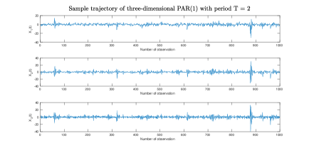
We mention here that an exact method for simulating the multidimensional $\alpha$-stable random vectors is presented in (Modarres and Nolan, 1994). In the simulation study presented here two PAR(1) models, denoted as Model 1 (two-dimensional PAR(1) model) and Model 2 (three-dimensional PAR(1) model), that correspond to $T=3$ and $T=2$, respectively, with the following coefficient matrices

$$\Theta(1)=\left[\begin{array}[]{cc}0.5&0.1\\ -0.6&0.4\\ \end{array}\right],\quad\Theta(2)=\left[\begin{array}[]{cc}0.8&-0.1\\ 0.3&0.7\\ \end{array}\right],\quad\Theta(3)=\left[\begin{array}[]{cc}0.1&-0.4\\ -0.5&0.3\\ \end{array}\right]$$ (37)

for Model 1, and

$$\Theta(1)=\left[\begin{array}[]{ccc}0.8&-0.2&0.7\\ 0.1&0.5&-0.6\\ 0.4&0.3&-0.1\\ \end{array}\right],\quad\Theta(2)=\left[\begin{array}[]{ccc}0.4&-0.1&0.3\\ 0.5&-0.2&0.4\\ -0.3&0.8&-0.6\end{array}\right]$$ (38)

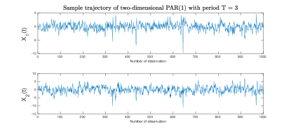
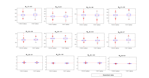
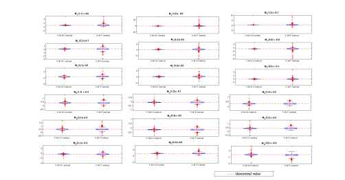
for Model 2. Sample trajectories of length $L=1000$ of the considered time series are given in Figs. 1 and 6 for Model 1 and Model 2 respectively. Next, we estimate PAR coefficient matrices for Model 1 and Model 2 using Y-W methods based on moment-based covariation (Y-W-CV method) and spectral measure-based covariation (Y-W-T method) given in Section 4. The results are obtained by both estimation method using the Monte-Carlo simulations, namely, for each model, we generate $M=1000$ trajectories of length $L=1000$. Also, we compare the estimated coefficient matrices using Y-W-CV method with using the Y-W-T method. In Figs. 2 and 7, we present the boxplots of the estimated coefficient matrices using both methods for Model 1 and Model 2, respectively. As one can see, the medians of the values taken by estimators using both methods are close to the real values of the coefficient matrices. We can observe that the Y-W-CV-based estimators are narrower in comparison to Y-W-T ones. Thus, the Y-W-CV method is preferable here and will be further used for real data analysis presented in the next section. From Figs. 2 and 7 one can suppose that the variances for the coefficients from different periods are different. There is no reason for that as all coefficients are estimated in the same way. This is due to the arrangement of the figures (i.e. application of different scales on the subplots) applied to compare the results between two estimation methods.

Figure 1: Sample trajectories of the two-dimensional $\alpha-$stable PAR(1) time series of length $L=1000$ with $T=3$ - Model 1. The coefficient matrices are given in Eq. (37), $\alpha=1.8$ and the spectral measure is defined in Eq. (35).

Figure 2: The boxplots of estimated coefficient matrices for the two-dimensional $\alpha-$stable PAR(1) time series of length length $L=1000$ with $T=3$ - Model 1. The coefficient matrices are given in Eq. (37), $\alpha=1.8$ and the spectral measure is defined in Eq. (35). The boxplots on left hand side of all panels describe the estimated coefficient matrices values using Y-W-CV method while the right boxplots using the Y-W-T method. The results are obtained by using Monte-Carlo simulations with the number of repetitions equal to $M=1000$.

Figure 3: The graph presenting the results (medians and 90% empirical confidence intervals using empirical quantiles function) for the Y-W-CV estimation method applied to the two-dimensional $\alpha-$stable PAR(1) time series of length $L=500$ with $T=3$ - Model 1. The coefficient matrices are given in Eq. (37), the spectral measure is defined in Eq. (35) and $\alpha$ is changing from $\alpha=1.1$ to $\alpha=1.9$. The results are obtained by using Monte-Carlo simulations with the number of repetitions equal to $M=1000$.

Figure 4: The graph presenting the results (medians and 90% empirical confidence intervals using empirical quantiles function) for the Y-W-CV estimation method applied to the two-dimensional $\alpha-$stable PAR(1) time series of length $L=1000$ with $T=3$ - Model 1. The coefficient matrices are given in Eq. (37), the spectral measure is defined in Eq. (35) and $\alpha$ is changing from $\alpha=1.1$ to $\alpha=1.9$. The results are obtained by using Monte-Carlo simulations with the number of repetitions equal to $M=1000$.

Figure 5: The graph presenting the results (medians and 90% empirical confidence intervals using empirical quantiles function) for the Y-W-CV estimation method applied to the two-dimensional $\alpha-$stable PAR(1) time series of length $L=2000$ with $T=3$ - Model 1. The coefficient matrices are given in Eq. (37), the spectral measure is defined in Eq. (35) and $\alpha$ is changing from $\alpha=1.1$ to $\alpha=1.9$. The results are obtained by using Monte-Carlo simulations with the number of repetitions equal to $M=1000$.

Figure 6: Sample trajectories of the three-dimensional $\alpha-$stable PAR(1) time series of length $L=1000$ with $T=2$ - Model 2. The coefficient matrices are given in Eq. (38), $\alpha=1.8$ and the spectral measure is defined in Eq. (36).

Figure 7: The boxplots of estimated coefficient matrices for the three-dimensional $\alpha-$stable PAR(1) time series of length length $L=1000$ with $T=2$ - Model 2. The coefficient matrices are given in Eq. (38), $\alpha=1.8$ and the spectral measure is defined in Eq. (36). The boxplots on left hand side of all panels describe the estimated coefficient matrices values using Y-W-CV method while the right boxplots using the Y-W-T method. The results are obtained by using Monte-Carlo simulations with the number of repetitions equal to $M=1000$.

Figure 8: The graph presenting the results (medians and 90% empirical confidence intervals using empirical quantiles function) for the Y-W-CV estimation method applied to the three-dimensional $\alpha-$stable PAR(1) time series of length $L=500$ with $T=2$ - Model 2. The coefficient matrices are given in Eq. (38), the spectral measure is defined in Eq. (36) and $\alpha$ is changing from $\alpha=1.1$ to $\alpha=1.9$. The results are obtained by using Monte-Carlo simulations with the number of repetitions equal to $M=1000$.

Figure 9: The graph presenting the results (medians and 90% empirical confidence intervals using empirical quantiles function) for the Y-W-CV estimation method applied to the three-dimensional $\alpha-$stable PAR(1) time series of length $L=1000$ with $T=2$ - Model 2. The coefficient matrices are given in Eq. (38), the spectral measure is defined in Eq. (36) and $\alpha$ is changing from $\alpha=1.1$ to $\alpha=1.9$. The results are obtained by using Monte-Carlo simulations with the number of repetitions equal to $M=1000$.

Figure 10: The graph presenting the results (medians and 90% empirical confidence intervals using empirical quantiles function) for the Y-W-CV estimation method applied to the three-dimensional $\alpha-$stable PAR(1) time series of length $L=2000$ with $T=2$ - Model 2. The coefficient matrices are given in Eq. (38), the spectral measure is defined in Eq. (36) and $\alpha$ is changing from $\alpha=1.1$ to $\alpha=1.9$. The results are obtained by using Monte-Carlo simulations with the number of repetitions equal to $M=1000$.

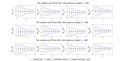
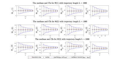
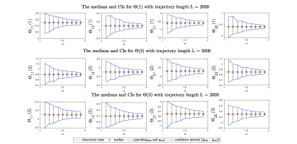
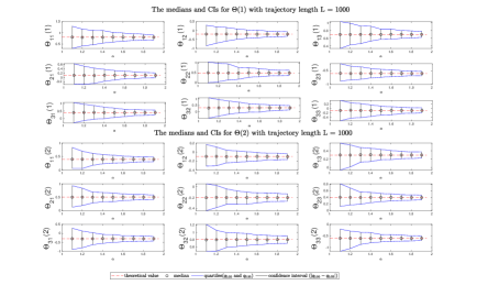
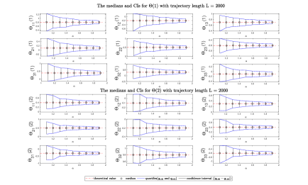
For the considered time series models, we want to evaluate the accuracy of the proposed Y-W-CV estimation procedure for different values of the stability index and different trajectory lengths. Therefore, for both models we generate $M=1000$ sample trajectories of the lengths $L$ with $\alpha$ changing from $\alpha=1.1$ to $\alpha=1.9$. Based on the simulated trajectories, we estimate the unknown coefficients of the model using the proposed Y-W-CV method. For the outcomes corresponding to each value of $\alpha$ we calculate the median and the quantiles of order $0.05$ and $0.95$ ($90\%$ empirical confidence intervals using empirical quantiles function). For Model 1 and Model 2, the results are presented in Figs. 3-5 and Figs. 8-10, respectively, for the trajectories of length $L=500$, $L=1000$ and $L=2000$. As one can observe, for both models the medians of the values taken by the estimated coefficients are close to theoretical ones and the length of the calculated empirical confidence intervals decreases if the values of $\alpha$ and $L$ increase.

6 Real data analysis

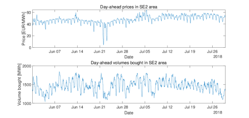
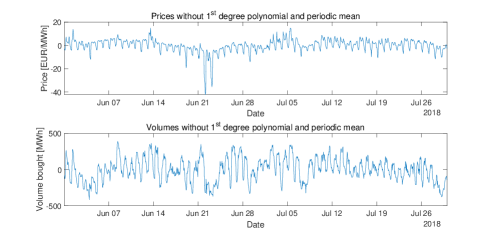
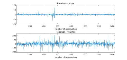
In this section, the application of the considered model to the real data is presented. The analyzed dataset comes from the Nord Pool power day-ahead market for the Swedish SE2 area and contains two hourly time series – prices (dat, a) and volumes bought (dat, b) – from 31st May 2018 through 29th July 2018 . In both trajectories, presented in Fig. 11, there are 1440 observations. The data are taken from the energy market and thus, we expect the periodic behavior related to the $T=24$, as we are considering hourly data and thus the periodic model is a natural choice. On the other hand, it is obvious that the prices and volumes bought are related. Thus, the two-dimensional model is proposed. Finally, the data are expected to be non-Gaussian (large observations are visible in both datasets). Thus, the $\alpha-$stable distribution seems to be justified for the distribution of the residual vector. From each trajectory, the fitted first-degree polynomial and the periodic mean are subtracted. To the data without these components, presented in Fig. 12, the two-dimensional $\alpha$-stable PAR(1) model with period $T$ is now fitted, using the Y-W-CV method introduced in Section 4. The estimated values for all $2\cdot 2\cdot 24=96$ coefficients are presented in Table 2 in Appendix C.

Figure 11: The analyzed dataset: hourly prices (top panel) and volumes bought (bottom panel) in Swedish SE2 area in the Nord Pool power day-ahead market from 31st May 2018 through 29th July 2018.

Figure 12: The analyzed prices (top panel) and volumes (bottom panel) series with the fitted first-degree polynomial and the periodic mean (with period $T=24$) subtracted.

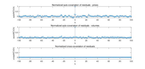
The obtained residual series are illustrated in Fig. 13. First, we check if each residual vector consists of independent observations. As we assume the residuals are $\alpha$-stable distributed, the auto-covariation measure is used. The top and middle panels of Figs. 14 present the estimated normalized auto-covariations for each residual vector. In both cases, there are no signs of a significant interdependence. However, one can see that the situation is not perfect. Especially for the price data the normalized auto-covariation takes no zero values for $h\neq 0$. The data are used here to demonstrate the possible applications of the presented methodology, and probably the proposed model is not the optimal one. However, it can be used as a preliminary description of the specific behavior visible in the data. Moreover, as one can see in the bottom panel of Fig. 14, the estimated values of normalized cross-covariation indicate that there is no dependence between the residual vector components. This is also confirmed by the estimated spectral measure presented in Fig. 17 in Appendix D.

Figure 13: The obtained residuals for prices (top panel) and volumes (bottom panel) series.

Figure 14: Top panel: normalized auto-covariation of prices’ residual series, middle panel: normalized auto-covariation of volumes’ residual series, bottom panel: normalized cross-covariation of residuals.

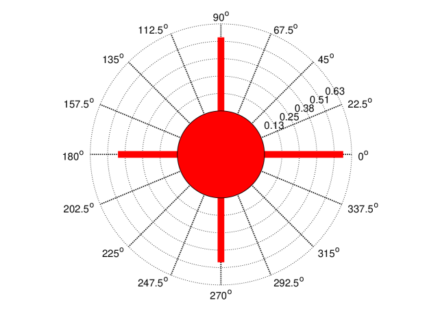
Next, we analyze the distribution of the residuals and check whether they can be considered as a sample of a two-dimensional $S\alpha S$ vector. Separately, for each residual series, the parameters of the $\alpha$-stable distribution are estimated using the McCulloch method (McCulloch, 1996). To confirm that both vectors can be treated as $\alpha$-stable distributed samples, we perform the Monte Carlo-based Anderson-Darling (A-D) test with 1000 simulations (Borak et al., 2011). The results are presented in Table 1. From the obtained empirical p-values, one can conclude that there is no reason to reject the hypothesis about the $\alpha$-stable distribution in both cases. Table 1 also contains the estimated values of the parameter $\alpha$ for both residual vector. One can see that they are close to each other hence one can claim the residuals constitute two-dimensional vector from $\alpha-$stable distribution. The estimated spectral measure corresponding to the residual vector (after the normalization by the estimated scale parameters) is presented in Fig. 17 given in Appendix D. The estimated point masses and weight suggest that the components of the two-dimensional $\alpha$-stable vector can be considered as independent. Moreover, the estimated spectral measure indicates that the measure is symmetric.

Table 1: Empirical p-values of the Anderson-Darling test based on 1000 Monte Carlo simulations and estimated values of stability index $\alpha$ for residual series.

residuals	p-value of A-D test	estimated value of $\alpha$
prices	0.2060	1.4095
volumes	0.1720	1.4103

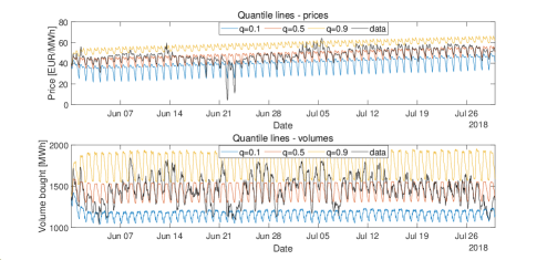
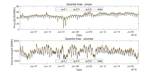
Finally, we have generated the quantile lines, using the following procedure. The 5000 trajectories of the two-dimensional $\alpha$-stable PAR(1) model with period $T=24$ and estimated parameters are simulated. The residuals are simulated from the two-dimensional $\alpha-$stable distribution with the estimated spectral measure and $\alpha$ parameter equal to the mean of the estimated stability indices obtained for components of the residual vector. Using these trajectories, we construct the quantile lines, taking quantiles of order $q=0.1,\,0.5,\,0.9$. To compare them with the original dataset, the previously subtracted deterministic components (first-degree polynomials and periodic means) are added to the simulated series. This comparison, illustrated in Fig. 15, confirms that the considered model can be used for description of the examined data. Moreover, in Fig. 16 we present also the one-step ahead conditional quantiles constructed based on the fitted model. This plot also confirms that the model is appropriate for the considered real data.

Figure 15: Quantile lines, based on the 5000 simulated trajectories of the two-dimensional $\alpha$-stable PAR(1) model with period $T=24$ and with estimated parameters (with added deterministic components) in comparison with the original dataset.

Figure 16: Quantile lines of one-step ahead predictions, based on the 5000 simulated trajectories of the two-dimensional $\alpha$-stable PAR(1) model with period $T=24$ and with estimated parameters (with added deterministic components) in comparison with the original dataset.

7 Conclusions and future study

In this paper, the multidimensional PAR model with infinite-variance distribution is considered. The special attention we have paid to new estimation methods dedicated to the model. These method are based on the generalized Yule-Walker equations where the classical auto- and cross-covariance functions are replaced by the auto- and cross-covariation functions, properly defined for the $\alpha-$stable models. The presented simulation results indicate the validity of the proposed methodology. Moreover, we compare the Y-W-CV method with Y-W-T method. The presented simulation study indicates the Y-W-CV technique is more effective than Y-W-T. However, one can conclude that the dispersion of the new estimator is still a challenging task. Finally, the new approach was applied for the real-time series to show the possible applications of the introduced methodology. Although the fitted model is not perfect for the analyzed data, the presented analysis demonstrates how to proceed in order to fit the multidimensional periodic model with non-Gaussian characteristics.

Although the new approach is introduced and its validity is examined in this paper, there are still a few important open questions. The first one is the proper identification of the model order. In the classical Gaussian case, there are known information criteria that can be useful here. Also in a one-dimensional infinite-variance case, several attempts have been made in this area (Kruczek et al., 2017a). However, according to our knowledge, there is still a space for the new algorithms of the proper model recognition for the multidimensional infinite-variance models. The second issue is the identification of the period $T$. In this paper for real data analysis, it is assumed that $T$ is known. However, for many real applications, this value is not given and needs to be estimated. In case when the data are Gaussian or finite-variance-distributed, there are known methods for period identification, like coherent or incoherent statistics based on the autocovariance function (Broszkiewicz-Suwaj et al., 2004). In the $\alpha-$stable case, the problem is much more complicated. One of the possible approaches is based on the replacement of the autocovariance function by the adequate dependency measure. The similar problem was discussed in (Kruczek et al., 2020) for vibration data. However this issue needs to be carefully investigated and thus, we decide to consider it as the future study.

The possible extension of the presented methodology is the introduction of the new estimation algorithms for the time-varying AR models when the assumption of Gaussian distribution is not valid. Thus, we see here a huge potential for further research and further application of the introduced methodology.

Data Availability Statement

Not applicable.

8 Declarations

Funding
The work of P. Giri and S. Sundar was supported by Indian Institute of Technology Madras, India under the Project No. SB20210848MAMHRD008558 ”Centre for Computational Mathematics and Data Science, Department of Mathematics, IIT Madras Chennai India”.
The work of A. Wyłomańska was supported by the National Center of Science under Opus Grant 2020/37/B/HS4/00120 ”Market risk model identification and validation using novel statistical, probabilistic, and machine learning tools”.
The work of W. Żuławiński was supported by National Center of Science under Sheng2 project No. UMO-2021/40/Q/ST8/00024 ”NonGauMech - New methods of processing non-stationary signals (identification, segmentation, extraction, modeling) with non-Gaussian characteristics for the purpose of monitoring complex mechanical structures”.
Conflicts of interest/Competing interests
The authors have no conflicts of interest to declare that are relevant to the content of this article.
Availability of data and material
The data were available and downloaded in September 2020.
Code availability
Not applicable
Authors’ contributions
Conceptualization: [ S. Sundar, A. Wylomanska, P. Giri, A. Grzesiek, W. Żuławiński], Methodology: [A. Wylomanska, P. Giri, A. Grzesiek], Formal analysis and investigation: [ P. Giri, A. Grzesiek, W. Żuławiński], Writing - original draft preparation: [P. Giri,A. Grzesiek, W. Żuławiński, A. Wylomanska]; Writing - review and editing: [P. Giri,A. Grzesiek, A. Wylomanska], Supervision: [S. Sundar, A. Wylomanska]

Appendix A The proof of Lemma 1

From [Samorodnitsky and Taqqu, 1994], the cross-covariation given in Eq. (7) can be calculated using the following formula

$$\mathrm{CV}(X_{r}(s),X_{l}(t))=\frac{1}{\alpha}\frac{\sigma^{\alpha}(\theta_{1},\theta_{2})}{\partial\theta_{1}}\bigg{\rvert}_{\theta_{1}=0,\theta_{2}=1},$$

where $\sigma^{\alpha}(\theta_{1},\theta_{2})$ denotes the scale parameter of $\theta_{1}X_{r}(s)+\theta_{2}X_{l}(t)$. Note that for $s\geq t$

$$\exp\{-\sigma^{\alpha} (\theta_{1},\theta_{2})\}={\mathrm{E}}\left[\exp\left\{i\left(\theta_{1}X_{r}(s)+\theta_{2}X_{l}(t)\right)\right\}\right]$$

$$=\exp\Bigg{\{}-\Bigg{(}\sum_{j=0}^{-(t-s)+1}\int_{S_{m}}|\theta_{1}g_{r1}(s,{s-j+1})s_{1}+\ldots+\theta_{m}g_{rm}(s,{s-j+1})s_{m}|^{\alpha}\Gamma(ds)$$

$$\hskip 28.45274pt+\sum_{j=-(t-s)}^{+\infty}\int_{S_{m}}|\left(\theta_{1}g_{r1}(s,{s-j+1})+\theta_{2}g_{l1}({t},{s-j+1})\right)s_{1}+\ldots$$

$$\hskip 28.45274pt+\big{(}\theta_{1}g_{rm}(s,{s-j+1})+\theta_{2}g_{lm}({t},{s-j+1})\big{)}s_{m}|^{\alpha}\Gamma(ds)\Bigg{)}\Bigg{\}}.$$

And consequently

$$\mathrm{CV}(X_{r}(s),X_{l}(t))=\sum_{j=0}^{+\infty}\int_{S_{m}}\left(g_{l1}({t},{t-j+1})s_{1}+g_{l2}({t},{t-j+1})s_{2}+\ldots+g_{lm}({t},{t-j+1})s_{m}\right)^{\langle\alpha-1\rangle}\\ \left(g_{r1}({s},{t-j+1})s_{1}+g_{r2}({s},{t-j+1})s_{2}+\ldots+g_{rm}({s},{t-j+1})s_{m}\right)\Gamma(ds).$$

By proceeding similarly one can show that for $s\leq t$

$$\mathrm{CV}(X_{r}(s),X_{l}(t))=\sum_{j=0}^{+\infty}\int_{S_{m}}\left(g_{l1}({t},{s-j+1})s_{1}+g_{l2}({t},{s-j+1})s_{2}+\ldots+g_{lm}({t},{s-j+1})s_{m}\right)^{\langle\alpha-1\rangle}\\ \left(g_{r1}({s},{s-j+1})s_{1}+g_{r2}({s},{s-j+1})s_{2}+\ldots+g_{rm}({s},{s-j+1})s_{m}\right)\Gamma(ds).$$

∎

Appendix B An Algorithms to solve system of equations

In this section, we present an algorithm (method) to solving the consistent system of equations (29). Since the normalized-covariation-based matrix is positive semi-definite matrix, therefore it can be singular or non-singular matrix i.e $\widehat{\mathbf{NCV}}^{(v-1)}(0)$ for each $v=1,\ldots,T$ can be singular or non-singular. If $\hat{NCV}^{(v-1)}(0)$ is singular and system of equations given in Eq. (29) are consistent. Then the solution $\hat{\Theta}(v)$ exists but it is not unique. So in this case, we need a numerical method for solving system of equations. There are many methods available in literature but in this paper we used the latest and very popular numerical method named by Bi-conjugate gradient stabilized method i.e BICGSTAB. This method can be use for non-singular case also. In both cases, we can use the following method (algorithm) to solve the system of equations (29).

procedure $SOLUTION_{1}$($\widehat{\mathbf{NCV}}^{(v-1)}(0)$ , $\widehat{\mathbf{NCV}}^{v}(1)$) $\triangleright$ where $\widehat{\mathbf{NCV}}^{(v-1)}(0)$ and $\widehat{\mathbf{NCV}}^{v}(1)$ are $m\times m$ matrices

     $A_{v}\leftarrow\widehat{\mathbf{NCV}}^{(v-1)}(0)^{\prime}$ $\triangleright$ where $\widehat{\mathbf{NCV}}^{(v-1)}(0)^{\prime}$ is transpose of $\widehat{\mathbf{NCV}}^{(v-1)}(0)$

     $B_{v}\leftarrow\widehat{\mathbf{NCV}}^{v}(1)^{\prime}$ $\triangleright$ where $\widehat{\mathbf{NCV}}^{v}(1)^{\prime}$ is transpose of $\widehat{\mathbf{NCV}}^{v}(1)$

     for $i=1,2$

     $\mathbf{\Theta_{v}}(:,i)\leftarrow BICGSTAB(A_{v},B_{v}(:,i),tol,maxit,M_{1},M_{2})$ $\triangleright$ where $\mathbf{\Theta_{v}}(:,i)$ is $i^{th}$ column of $\mathbf{\Theta_{v}}$ and $M=M_{1}M_{2}\sim A_{v}$ is preconditioned.

     end

     $\mathbf{\Theta}_{v}\leftarrow\mathbf{\Theta}_{v}^{\prime}$ $\triangleright$ where $\mathbf{\Theta}_{v}=\mathbf{\Theta}(v)$

     return $\mathbf{\Theta}(v)$

Algorithm 1 The algorithm to solving system of equation (29)

where $BICGSTAB$ is a method (algorithm) with preconditioned to solve linear system of equations A x = b (say), where A is coefficient matrix whether A can be singular or non-singular, x is vector of unknown and b is known vector. It is latest and updated method. For more details of $BICGSTAB$ see [Ocłoń et al., 2013, Saad, 2003, Barrett et al., 1994, van der Vorst, 1992].

Appendix C Values of estimated parameters for the analyzed data

Table 2: Estimated values of the fitted model’s parameters.

$v$	$\widehat{\Theta}_{11}(v)$	$\widehat{\Theta}_{12}(v)$	$\widehat{\Theta}_{21}(v)$	$\widehat{\Theta}_{22}(v)$
1	1.0226	0.0014	1.8911	0.9637
2	1.0560	0.0005	0.6924	0.9514
3	1.0896	0.0014	-0.1668	0.9449
4	1.0284	-0.0026	-0.6131	0.9920
5	0.7265	0.0054	-1.4507	0.9904
6	0.7508	0.0001	4.3211	0.9230
7	0.9214	-0.0002	11.4943	0.8547
8	1.0841	0.0009	6.7091	1.0086
9	0.9445	-0.0029	-1.5941	0.9819
10	0.9374	-0.0007	0.7084	0.9002
11	1.0180	-0.0007	-4.2928	1.0619
12	0.8873	-0.00003	-0.7590	0.9210
13	0.9757	0.0026	3.5708	0.9038
14	0.9979	-0.0004	-1.6383	1.0344
15	1.0264	-0.0017	1.0125	0.9504
16	0.9862	-0.0019	-2.6817	0.9845
17	0.9803	0.0010	-3.9416	0.9087
18	1.0461	0.0007	8.0590	0.7278
19	0.9967	-0.0004	2.2757	0.9442
20	0.9141	-0.0005	1.2990	0.8396
21	0.9555	-0.00003	-2.3115	0.9922
22	0.9654	0.0005	0.7507	0.9437
23	1.0466	-0.0015	0.8990	0.9548
24	1.0265	0.0004	0.0823	0.7418

Appendix D Estimated spectral measure

Figure 17: Estimated spectral measure for the residual series (with normalized components) of the fitted model.

References

- dat [a] [dataset] Nord Pool. Hourly day-ahead prices in SE2 area, 31st May 2018 - 29th July 2018. https://www.nordpoolgroup.com/en/Market-data1/Dayahead/Area-Prices/ALL1/Hourly/ (column SE2), a.
- dat [b] [dataset] Nord Pool. Hourly day-ahead volumes bought in SE2 area, 31st May 2018 - 29th July 2018. https://www.nordpoolgroup.com/en/Market-data1/Dayahead/Volumes/ALL1/Hourly11/ (column SE2 Buy), b.
- Adams and Goodwin [1995] G. J. Adams and G. C. Goodwin. Parameter estimation for periodic ARMA models. J. Time Ser. Anal., 16(2):127–145, 1995.
- Alj et al. [2017] A. Alj, R. Azrak, C. Ley, and G. Mélard. Asymptotic properties of QML estimators for VARMA models with time-dependent coefficients. Scand. J. Stat., 44(3):617–635, 2017.
- Anderson and Meerschaert [2005] P. L. Anderson and M. M. Meerschaert. Parameter estimation for periodically stationary time series. J. Time Ser. Anal., 26(4):489–518, 2005.
- Anderson et al. [2013] P. L. Anderson, M. M. Meerschaert, and K. Zhang. Forecasting with prediction intervals for periodic autoregressive moving average models. J. Time Ser. Anal., 34(2):187–193, 2013.
- Antoni [2009] J. Antoni. Cyclostationarity by examples. Mech. Syst. Signal Process., 23(4):987–1036, 2009.
- Antoni et al. [2004] J. Antoni, F. Bonnardot, A. Raad, and M. El Badaoui. Cyclostationary modelling of rotating machine vibration signals. Mech. Syst. Signal Process., 18(6):1285–1314, 2004.
- Barrett et al. [1994] R. Barrett, M. Berry, T. Chan, J. Demmel, J. Donato, J. Dongarra, V. Eijkhout, R. Pozo, C. Romine, and H. van der Vorst. Templates for the Solution of Linear Systems: Building Blocks for Iterative Methods. Society for Industrial and Applied Mathematics, 1994.
- Basawa and Lund [2001] I. V. Basawa and R. Lund. Large sample properties of parameter estimates for periodic ARMA models. J. Time Ser. Anal., 22(6):651–663, 2001.
- Bertha and Golinval [2017] M. Bertha and J.-C. Golinval. Identification of non-stationary dynamical systems using multivariate ARMA models. Mech. Syst. Signal Process., 88:166–179, 2017.
- Bloomfield et al. [1994] P. Bloomfield, H. Hurd, and R. Lund. Periodic correlation in stratospheric ozone time series. J. Time Ser. Anal., 15:127–150, 1994.
- Borak et al. [2011] S. Borak, A. Misiorek, and R. Weron. Models for heavy-tailed asset returns. In Statistical Tools for Finance and Insurance, pages 21–55. Springer, 2011.
- Brelsford and Jones [1967] M. Brelsford and R. Jones. Time series with periodic structure. Biometrika, 54:403–407, 1967.
- Brockwell et al. [2012] P. Brockwell, A. Lindner, and B. Vollenbroeker. Strictly stationary solutions of multivariate ARMA equations with i.i.d. noise. Ann. Inst. Stat. Math., 64:1089–1119, 2012.
- Brockwell and Davis [2002] P. J. Brockwell and R. A. Davis. Introduction to Time Series and Forecasting. New York: Springer, 2002.
- Broszkiewicz-Suwaj et al. [2004] E. Broszkiewicz-Suwaj, A. Makagon, R. Weron, and A. Wyłomańska. On detecting and modeling periodic correlation in financial data. Physica A, 336(1-2):196–205, 2004.
- Bukofzer [1987] D. Bukofzer. Optimum and suboptimum detector performance for signals in cyclostationary noise. J. Ocean. Eng., 12:97–115, 1987.
- Byczkowski et al. [1993] T. Byczkowski, J. P. Nolan, and R. B. Approximation of multidimensional stable densitiess. Journal of Multivariate Analysis, 46:13–31, 1993.
- Chen et al. [2018] Z. Chen, S. X. Ding, T. Peng, C. Yang, and W. Gui. Fault detection for non-Gaussian processes using generalized canonical correlation analysis and randomized algorithms. IEEE Trans. Ind. Electron., 65(2):1559–1567, 2018.
- Cheng and Rachev [1995] B. N. Cheng and S. T. Rachev. Multivariate stable futures prices. Mathematical Finance, 5(2):133–153, 1995.
- Dargaville et al. [2003] R. Dargaville, S. Doney, and I. Fung. Inter-annual variability in the interhemispheric atmospheric CO2 gradient. Tellus B, 15:711–722, 2003.
- Donohue et al. [1993] K. Donohue, J. Bressler, T. Varghese, and N. Bilgutay. Spectral correlation in ultrasonic pulse-echo signal processing. IEEE Trans. Ultrason. Ferroelectr. Freq. Control, 40:330–337, 1993.
- Fellingham and Sommer [1984] L. Fellingham and F. Sommer. Ultrasonic characterization of tissue structure in the in vivo human liver and spleen. IEEE Trans. Sonics Ultrason., 31:418–428, 1984.
- Franses [1996] P. Franses. Periodicity and Stochastic Trends in Economic Time Series. Oxford University Press, Oxford, 1996.
- Gallagher [2001] C. M. Gallagher. A method for fitting stable autoregressive models using the autocovariation function. Stat. Probab. Lett., 53:381–390, 2001.
- Gladyshev [1961] E. G. Gladyshev. Periodically correlated random sequences. Sov. Math., 2:385–388, 1961.
- Gosoniu et al. [2006] L. Gosoniu, P. Vounatsou, N. Sogoba, and T. Smith. Bayesian modelling of geostatistical malaria risk data. Geospat. Health, 1(1):127–139, 2006.
- Grzesiek and Wyłomańska [2019] A. Grzesiek and A. Wyłomańska. Asymptotic behavior of the cross-dependence measures for bidimensional AR(1) model with stable noise. Accepted in Banach Center Publ., 2019. , Located at: https://arxiv.org/abs/1911.10894.
- Grzesiek et al. [2019a] A. Grzesiek, S. Sundar, and A. Wyłomańska. Fractional lower order covariance-based estimator for bidimensional AR(1) model with stable distribution. Int. J. Adv. Eng. Sci. Appl. Math., 11:217–229, 2019a.
- Grzesiek et al. [2019b] A. Grzesiek, M. Teuerle, and A. Wyłomańska. Cross-codifference for bidimensional VAR(1) models with infinite variance. Published online in Commun. Stat. Simul. Comput., 2019b. doi: 10.1080/03610918.2019.1670840.
- Grzesiek et al. [2020a] A. Grzesiek, P. Giri, S. Sundar, and A. Wyłomańska. Measures of cross-dependence for bidimensional periodic AR(1) model with stable distribution. Accepted in J. Time Ser. Anal., 2020a. doi: 10.1111/jtsa.12548.
- Grzesiek et al. [2020b] A. Grzesiek, M. Teuerle, G. Sikora, and A. Wyłomańska. Spatial-temporal dependence measures for stable bivariate AR(1). J. Time Ser. Anal., 41(3):454–475, 2020b.
- Guzdenko [1959] L. Guzdenko. The small fluctuation in essentially nonlinear autooscillation system. Dokl. Akad. Nauk USSR, 125:62–65, 1959.
- Hallin and Saidi [2005] M. Hallin and A. Saidi. Testing non-correlation and non-causality between multivariate ARMA time series. J. Time Ser. Anal., 26(1):83–105, 2005.
- Hipel and McLeod [1994] K. W. Hipel and A. I. McLeod. Chapter 14 Periodic Models. In Time Series Modelling of Water Resources and Environmental Systems, volume 45 of Developments in Water Science, pages 483–524. Elsevier, 1994.
- Jachan et al. [2007] M. Jachan, G. Matz, and F. Hlawatsch. Time-frequency ARMA models and parameter estimators for underspread nonstationary random processes. IEEE Trans. Signal Process., 55(9):4366–4381, 2007.
- Jones and Brelsford [1968] R. Jones and W. Brelsford. Time series with periodic structure. Biometrika, 54:403–408, 1968.
- Kang [1981] H. Kang. Necessary and sufficient conditions for causality testing in multivariate ARMA models. J. Time Ser. Anal., 2(2):95–101, 1981.
- Kokoszka and Taqqu [1997] P. Kokoszka and M. Taqqu. The asymptotic behavior of quadratic forms in heavy-tailed strongly dependent random variables. Stoch. Process. Their Appl., 66:21–40, 1997.
- Kruczek et al. [2017a] P. Kruczek, A. Wyłomańska, M. Teuerle, and J. Gajda. The modified Yule-Walker method for alpha-stable time series models. Physica A, 469:588–603, 2017a.
- Kruczek et al. [2017b] P. Kruczek, A. Wyłomańska, M. Teuerle, and J. Gajda. The modified Yule-Walker method for alpha-stable time series models. Physica A, 469:588––603, 2017b.
- Kruczek et al. [2019] P. Kruczek, W. Żuławiński, P. Pagacz, and A. Wyłomańska. Fractional lower order covariance based-estimator for Ornstein-Uhlenbeck process with stable distribution. Math. Appl., 47(2):259–292, 2019.
- Kruczek et al. [2020] P. Kruczek, R. Zimroz, and A. Wyłomańska. How to detect the cyclostationarity in heavy-tailed distributed signals. Signal Process., 172:107514, 2020.
- Lund and Basawa [2000] R. Lund and I. V. Basawa. Recursive prediction and likelihood evaluation for periodic ARMA models. J. Time Ser. Anal., 21(1):75–93, 2000.
- Makagon et al. [2004] A. Makagon, A. Weron, and A. Wyłomańska. Bounded solutions for ARMA model with varying coefficients. Applicationes Mathematicae, 31:273–285, 2004.
- McCulloch [1995] J. McCulloch. Estimation of bivariate stable spectral representation by the projection method. Computational Economics, 16:47–62, 1995.
- McCulloch [1996] J. H. McCulloch. Financial applications of stable distributions. In Statistical Methods in Finance, volume 14 of Handbook of Statistics, pages 393–425. Elsevier, 1996.
- Miller [1978] G. Miller. Properties of certain symmetric stable distributions. J. Multivar. Anal., 8(3):346–360, 1978.
- Mittnik and Rachev [2000] S. Mittnik and S. T. Rachev. Stable Paretian Models in Finance. New York: Wiley, 2000.
- Modarres and Nolan [1994] R. Modarres and J. P. Nolan. A method for simulating stable random vectors. Comput. Stat., 9:11–19, 1994.
- Mohammadi et al. [2015] M. Mohammadi, A. Mohammadpour, and H. Ogata. On estimating the tail index and the spectral measure of multivariate -stable distributions. Metrika: International Journal for Theoretical and Applied Statistics, 78(5):549–561, 2015.
- Nolan et al. [2001] J. Nolan, A. Panorska, and J. McCulloch. Estimation of stable spectral measures. Mathematical and Computer Modelling, 34(9):1113–1122, 2001.
- Nowicka and Wyłomańska [2006] J. Nowicka and A. Wyłomańska. The dependence structure for PARMA models with alpha-stable innovations. Acta Phys. Pol. B, 37(11):3071–3081, 2006.
- Nowicka-Zagrajek and Weron [2002] J. Nowicka-Zagrajek and R. Weron. Modeling electricity loads in California: ARMA models with hyperbolic noise. Signal Process., 82(12):1903–1915, 2002.
- Ocłoń et al. [2013] P. Ocłoń, S. Łopata, and M. Nowak. Comparative study of conjugate gradient algorithms performance on the example of steady-state axisymmetric heat transfer problem. Arch. Thermodyn., (3):15–44, 2013.
- Ogata [2013] H. Ogata. Estimation for multivariate stable distributions with generalized empirical likelihood. Journal of Econometrics, 172(2):248–254, 2013.
- Palacios and Steel [2006] M. B. Palacios and M. F. J. Steel. Non-Gaussian Bayesian geostatistical modeling. J. Am. Stat. Assoc., 101(474):604–618, 2006.
- Peiris [1988] M. S. Peiris. On the prediction of multivariate ARMA processes with a time dependent covariance structure. Commun. Stat. Theory Methods, 17(1):27–37, 1988.
- Peiris and Thavansewaran [2001] M. S. Peiris and A. Thavansewaran. Multivariate stable ARMA processes with time dependent coefficients. Metrika, 54:131–138, 2001.
- Pivato and Seco [2003] M. Pivato and L. Seco. Estimating the spectral measure of a multivariate stable distribution via spherical harmonic analysis. Journal of Multivariate Analysis, 87(2):219–240, 2003.
- Saad [2003] Y. Saad. Iterative Methods for Sparse Linear Systems. Society for Industrial and Applied Mathematics, 2003.
- Samorodnitsky and Taqqu [1994] G. Samorodnitsky and M. S. Taqqu. Stable Non-Gaussian Random Processes: Stochastic Models with Infinite Variance. New York: Chapman & Hall, 1994.
- Santos and Scotto [2019] I. Santos, C. Pereira and M. Scotto. On the theory of periodic multivariate INAR processes. Statistical Papers, 2019.
- Sathe and Upadhye [2020] A. M. Sathe and N. S. Upadhye. Estimation of the parameters of multivariate stable distributions. Communications in Statistics - Simulation and Computation, 2020. Published Online. DOI: 10.1080/03610918.2020.1784432.
- Shao and Lund [2004] Q. Shao and R. Lund. Computation and characterization of autocorrelations and partial autocorrelations in periodic ARMA models. J. Time Ser. Anal., 25(3):359–372, 2004.
- Sivakumar [2017] B. Sivakumar. Chaos in Hydrology: Bridging Determinism and Stochasticity. Dordrecht: Springer, 2017.
- Swift [1990] A. L. Swift. Orders and initial values of non-stationary multivariate ARMA models. J. Time Ser. Anal., 11(4):349–359, 1990.
- Takayasu [1984] H. Takayasu. Stable distribution and Lévy process in fractal turbulence. Prog. Theor. Phys., 72(3):471–479, 1984.
- Troutman [1979] B. Troutman. Some results in periodic autoregression. Biometrika, 66:219–228, 1979.
- Tzafestas [1985] S. Tzafestas. Multidimensional Systems - Techniques and Applications. New York: M.Dekker, 1985.
- Ula [1990] T. A. Ula. Periodic covariance stationarity of multivariate periodic autoregressive moving average processes. Water Resour. Res., 26(5):855–861, 1990.
- Ula [1993] T. A. Ula. Forecasting of multivariate periodic autoregressive moving-average processes. J. Time Ser. Anal., 14(6):645–657, 1993.
- Ursu and Turkman [2012] E. Ursu and K. F. Turkman. Periodic autoregressive model identification using genetic algorithms. J. Time Ser. Anal., 33(3):398–405, 2012.
- van der Vorst [1992] H. van der Vorst. Bi-CGSTAB: A fast and smoothly converging variant of Bi-CG for the solution of nonsymmetric linear systems. SIAM J. Sci. Stat. Comput., 13(2):631–644, 1992.
- Weron [1984] A. Weron. Stable processes and measures; a survey. In D. Szynal and A. Weron, editors, Probability Theory on Vector Spaces III, pages 306–364, Berlin, Heidelberg, 1984. Springer.
- Żak et al. [2017] G. Żak, A. Wyłomańska, and R. Zimroz. Data driven iterative vibration signal enhancement strategy using alpha-stable distribution. Shock. Vib., Article ID 3698370:11 pages, 2017.
- Żak et al. [2019] G. Żak, A. Wyłomańska, and R. Zimroz. Periodically impulsive behaviour detection in noisy observation based on generalised fractional order dependency map. Appl. Acoust., 144:31–39, 2019.
- Zielinski et al. [2008] J. Zielinski, N. Bouaynaya, D. Schonfeld, and W. O’Neill. Time-dependent ARMA modeling of genomic sequences. BMC Bioinform., 9 (Suppl 9):S14, 2008.
- Zolotarev [1986] V. M. Zolotarev. One-dimensional stable distributions. Translations of Mathematical Monographs. Providence: American Mathematical Society, 1986.