Well-posedness of a Nonlinear Acoustics – Structure Interaction Model

Barbara Kaltenbacher, Amjad Tuffaha
Abstract

We establish local-in-time and global in time well-posedness for small data, for a coupled system of nonlinear acoustic structure interactions. The model consists of the nonlinear Westervelt equation on a bounded domain with non homogeneous boundary conditions, coupled with a 4th order linear equation defined on a lower dimensional interface occupying part of the boundary of the domain, with transmission boundary conditions matching acoustic velocities and acoustic pressures. While the well-posedness of the Westervelt model has been well studied in the literature, there has been no works on the literature on the coupled structure acoustic interaction model involving the Westervelt equation. Another contribution of this work, is a novel variational weak formulation of the linearized system and a consideration of various boundary conditions.


Department of Mathematics
University of Klagenfurt
Klagenfurt, Austria
e-mail: barbara.kaltenbacher@aau.at


Department of Mathematics
American University of Sharjah
Sharjah, UAE
e-mail: atufaha@aus.edu


1 Introduction

In this paper, we study the interaction of a nonlinear acoustic fluid or gas with an elastic plate, a situation that is practically relevant, e.g., in the context of high intensity ultrasound; think, e.g., of a cavity enclosed by a thin wall [5] or a thin structure immersed in an ultrasound cleaning device [43].

One of the classical models of nonlinear acoustics (and probably the most widely used one) is the Westervelt equation [49], a quasilinear second order damped wave equation. For its analysis in the practically relevant case of a smooth bounded domain $\Omega$ we refer to, e.g., [28, 25, 21, 38, 47]; the free space case $\Omega=\mathbb{R}^{3}$ is considered in, e.g., [10] and local in time results for vanishing damping can be found in, e.g., [13, 11, 29]. Advanced models such as Kuznetsov’s equation [32], the Jordan-Moore-Gibson-Thompson (JMGT) equation [19, 41, 48, 45] and the Blackstock-Crighton-Brunnhuber-Jordan (BCBJ) equation [4, 8, 6] have been analyzed in, e.g., [10, 11, 20, 22, 21, 23, 24, 29, 26, 27, 38, 40].

For some recent work on the mathematical analysis of acoustics-structure interaction problems we refer to, e.g., [1, 2, 3, 34, 35] and the references therein. Most of these models involve a linear or semi-linear wave equation coupled with linear and nonlinear plate models. Another important aspect in the study of the mathematics of acoustics-structure interactions is control analysis, see for example [16, 17, 37, 50]. However, to the best of the authors’ knowledge, there are no results on well-posedness of nonlinear acoustics-structure interaction models involving the Westervelt equation.

The model we consider consists of the Westervelt equation defined on a bounded domain and coupled with a 4th order linear plate equation defined on a lower dimensional interface occupying a part of the boundary of the domain. The coupling is realized through the acoustic pressure which acts as a lifting force on the structural plate equation, in addition to a velocity matching condition involving the normal pressure gradient. We also consider the possibility of mixed type non-homogeneous boundary conditions on the rest of the boundary such as Dirichlet, Neumann, and absorbing boundary conditions. Well-posedness of the Westervelt equations under these various mixed boundary conditions were considered in [12] with vanishing boundary data. Considering non-zero boundary data, we aim at laying the foundations for practically relevant control problems in future research.

Our main result in this paper, is firstly the existence of energy level weak solutions for the linearized model, and secondly the existence of local and global-in-time smooth solutions for the full nonlinear model. In particular, we provide a novel variational formulation of the coupled problem, that allows us to analyze the linearized problem (Proposition 3.5 and Corollary 3.7). Using this together with a fixed point argument, we establish local and global in time well-posedness for sufficiently small data (Theorem 4.4). Challenges in the analysis of the model arise due to the well-known potential degeneracy of the Westervelt equation (which it shares with basically all other models of nonlinear acoustics) in addition to the low regularity due to mixed boundary conditions. In particular, coupling to the plate provides less regularity than, e.g., prescribed Dirichlet or Neumann boundary values would do. This requires a different approach as compared to the existing literature on the analysis of the Westervelt equation, e.g., [28, 39, 40]. We note that in the mixed Dirichlet/Neumann boundary conditions, additional assumptions on the domain have to be imposed since classical elliptic regularity does not hold in general [44, 46]. This assumption allows us to control the $L^{\infty}$ norm of the pressure and hence avoid degeneracy without having to control the full Sobolev norm.

The paper is organized as follows. Section 2 introduces the model and Section 3 provides the analysis of its linearization. In Section 4 we prove well-posedness of the nonlinear acoustics – plate model and in Section 5 we give a brief outlook on related further research questions.

1.1 Notation

We will use the function space $H^{2}_{\Delta}(\Omega):=\{u\in L^{2}(\Omega)\,:\,u\in L^{2}(\Omega),\,\Delta u\in L^{2}(\Omega)\}\supset H^{2}(\Omega)$

Moreover, we abbreviate by $C^{\Omega}_{\Gamma}$ the constant in the Poincaré-Friedrichs type inequality

$$\|v\|_{H^{1}(\Omega)}\leq C^{\Omega}_{\Gamma}\Bigl{(}\|\nabla v\|_{L^{2}(\Omega)}^{2}+\|v\|_{L^{2}(\Gamma)}^{2}\Bigr{)}^{1/2}\text{ for all }v\in H^{1}(\Omega)$$ (1.1)

for some regular boundary part $\Gamma\subseteq\partial\Omega$ with nonvanishing measure.

The norm of some continuous embedding $X(\Omega)\to Y(\Omega)$ for some Sobolev or Lebesgue spaces $X(\Omega)$, $X(\Omega)$ will be denoted by $C^{\Omega}_{X,Y}$.

We will sometimes drop the subscript in $\|\cdot\|_{L^{2}(\Omega)}$ (but not in the boundary norms, since this could cause confusion) and skip the trace operator whenever it is clear that we are taking some boundary trace of a function defined in $\Omega$.

The topological dual of a normed space $X$ will be denoted by $X^{\star}$.

2 Model

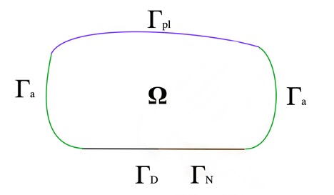
We consider a system of partial differential equations modeling the interaction between nonlinear acoustic waves and an isotropic, homogeneous plate. We take a domain $\Omega\subset\mathbb{R}^{3}$ with a $C^{1}$ boundary $\partial\Omega$ consisting of four different parts $\Gamma_{pl}$, $\Gamma_{a}$, $\Gamma_{D}$ and $\Gamma_{N}$, the plate coupling, absorbing, and excitation boundary parts, respectively. Each of these boundary parts is assumed to be regular in the sense that it is either empty or has positive measure and the interfaces between them are assumed to be Lipschitz curves. An exemplary geometric setup is depicted in figure 1.

Refer to caption
Figure 1: Domain setup (example)

The model consists of the Westervelt equation defined in the variable $p$ representing acoustic pressure

$\displaystyle(1-2kp)p_{tt}-c^{2}\Delta p-b\Delta p_{t}=2k(p_{t})^{2}~{}~{}\mbox{in}~{}~{}\Omega\times[0,T]$ (2.1)

and a $4$th order plate equation defined on $\Gamma_{pl}$ in the mid surface displacement variable $w$, forced by the trace of the pressure variable $p$

$\displaystyle\rho w_{tt}+\delta\Delta_{pl}^{2}w+\beta(-\Delta_{pl})^{\gamma}w_{t}=\kappa p+h~{}~{}$ $\displaystyle\mbox{on}~{}~{}\Gamma_{pl}\times[0,T],$ (2.2)

where $\Delta_{pl}$ is the Laplace-Beltrami operator on $\Gamma_{pl}$, equipped with homogeneous Dirichlet boundary conditions, and $h$ is a given forcing function. 111See, e.g., [35] for this type of coupling in a velocity potential formulation (rather than the pressure formulation we are using here). Here, the constants $\rho>0$, $c>0$, $\delta>0$ represent the mass density, the speed of sound and the ratio of plate stiffness to plate thickness respectively, while $b>0$, $\beta>0$, and $\gamma\geq 0$ are damping parameters. The parameter $\kappa>0$ is a coupling coefficient and $k$ is the nonlinearity parameter of the acoustic medium. The operator $(-\Delta_{pl})^{\gamma}$ is the spectrally defined power of the symmetric positive definite operator $(-\Delta_{pl})$; for its definition, see, e.g., [36, Section 2.1.1].

Accordingly, the boundary conditions we assume on the plate are of hinged type:

$\displaystyle w=\Delta_{pl}w=0~{}~{}\mbox{on}~{}~{}\partial\Gamma_{pl}\times[0,T].$ (2.3)

We also impose another boundary condition connecting the plate equation and the Westervelt equation which ensures continuity of inertial forces across the interface

$\displaystyle\partial_{\nu}{p}=-\rho w_{tt}~{}~{}$ $\displaystyle\mbox{on}~{}~{}\Gamma_{pl}\times[0,T].$ (2.4)

Note that the pressure $p$ is related to the particle velocity $v$ through the (linearized) momentum balance $\rho_{fl}v_{t}=-\nabla p$ where $\rho_{fl}$ is the mass density of the fluid.

On the boundary component $\Gamma_{a}$, we impose the absorbing boundary conditions

$\displaystyle p_{t}+c\partial_{\nu}{p}=a~{}~{}$ $\displaystyle\mbox{on}~{}~{}\Gamma_{a}\times[0,T]$ (2.5)

where the typical value of the boundary function is $a\equiv 0$ in order to avoid spurious reflections on the boundary of the computational domain $\Omega$, see, e.g., the review articles [14, 18] and the references therein.

Finally, we allow for mixed Dirichlet and/or Neumann boundary condition on the boundary components $\Gamma_{D}$ and $\Gamma_{N}$,

$$p=g_{D}~{}~{}\mbox{on}~{}~{}\Gamma_{D}\times[0,T]$$ (2.6)
$$\partial_{\nu}{p}=g_{N}~{}~{}\mbox{on}~{}~{}\Gamma_{N}\times[0,T],$$ (2.7)

where $g_{D}$ and $g_{N}$ are given functions. Subsets with $g_{D}=0$ and $g_{N}=0$ correspond to sound-soft and sound-hard boundary parts, respectively; nonvanishing values of $g_{D}$ and $g_{N}$ represent an excitation control action; in case of Neumann conditions, e.g., by some piezoelectric transducer array in ultrasonics.

Remark 2.1 (damping).

While the damping term in the plate equation is not needed for part of the well-posedness analysis, it is useful to achieve independence of estimates on the final time $T$ and to extract additional regularity of $p$ via the interface identity (3.10), see Remark 4.5 below.

On the contrary, strong damping in the Westervelt equation is essential even for only local in time well-posedness, since due to the lack of spatial regularity resulting from the mixed boundary conditions, the techniques from, e.g., [13, 29] would not be applicable here.

3 Linearized Model

3.1 Reformulation, Linearization, and some Auxiliary Results

We will reformulate the model in terms of $\widetilde{w}$ defined as

$\displaystyle\widetilde{w}=w_{tt}$ (3.8)

so that the boundary conditions on $\Gamma_{pl}$ are written as

$\displaystyle\rho\widetilde{w}_{tt}+\delta\Delta_{pl}^{2}\widetilde{w}+\beta(-\Delta_{pl})^{\gamma}\widetilde{w}_{t}=\kappa p_{tt}+\widetilde{h}~{}~{}$ $\displaystyle\mbox{on}~{}~{}\Gamma_{pl}\times[0,T]$ (3.9)

with $\widetilde{h}=h_{tt}$ and

$\displaystyle\partial_{\nu}{p}=-\rho\widetilde{w}~{}~{}$ $\displaystyle\mbox{in}~{}~{}\Gamma_{pl}\times[0,T].$ (3.10)

We also start our analysis on a linear variable coefficient version of (2.1)

$\displaystyle\alpha\,p_{tt}-c^{2}\Delta p-b\Delta p_{t}=f~{}~{}\mbox{in}~{}~{}\Omega\times[0,T]$ (3.11)

(having in mind $\alpha=\alpha(t,x)=(1-2kp)$, $f=f(t,x)=2k(p_{t})^{2}$), thus altogether

$\displaystyle\alpha\,p_{tt}-c^{2}\Delta p-b\Delta p_{t}$ $\displaystyle=f~{}~{}\mbox{in}~{}~{}\Omega\times[0,T]$ (3.12)
$\displaystyle c\partial_{\nu}{p}+p_{t}$ $\displaystyle=a~{}~{}\mbox{in}~{}~{}\Gamma_{a}\times[0,T]$
$\displaystyle p$ $\displaystyle=g_{D}~{}~{}\mbox{on}~{}~{}\Gamma_{D}\times[0,T]$
$\displaystyle\partial_{\nu}{p}$ $\displaystyle=g_{N}~{}~{}\mbox{on}~{}~{}\Gamma_{N}\times[0,T]$
$\displaystyle\partial_{\nu}{p}$ $\displaystyle=-\rho\widetilde{w}~{}~{}\mbox{on}~{}~{}\Gamma_{pl}\times[0,T]$
$\displaystyle\rho\widetilde{w}_{tt}+\delta\Delta_{pl}^{2}\widetilde{w}+\beta(-\Delta_{pl})^{\gamma}\widetilde{w}_{t}$ $\displaystyle=\kappa p_{tt}+\widetilde{h}~{}~{}\mbox{on}~{}~{}\Gamma_{pl}\times[0,T]$
$\displaystyle\widetilde{p}(0)$ $\displaystyle=p_{0},~{}~{}\widetilde{p}_{t}(0)=p_{1}.$

We homogenize the Dirichlet and Neumann conditions on $\Gamma_{D}$, $\Gamma_{N}$ as well as the absorbing condition on $\Gamma_{a}$ in order to be able to consider $g_{D}=0$, $g_{N}=0$, $a=0$ in the following. To this end, we decompose the solution $p$ into $\bar{p}$ and $\widetilde{p}$ where $\bar{p}$ serves as an extension of the inhomogeneous boundary data $g_{D}$, $g_{N}$, $a$ to the interior by satisfying the initial boundary value problem IBVP

$\displaystyle\alpha\,\bar{p}_{tt}-c^{2}\Delta\bar{p}-b\Delta\bar{p}_{t}$ $\displaystyle=0~{}~{}\mbox{in}~{}~{}\Omega\times[0,T]$ (3.13)
$\displaystyle c\partial_{\nu}{\bar{p}}+\bar{p}_{t}$ $\displaystyle=a~{}~{}\mbox{in}~{}~{}\Gamma_{a}\times[0,T]$
$\displaystyle\bar{p}$ $\displaystyle=g_{D}~{}~{}\mbox{on}~{}~{}\Gamma_{D}\times[0,T]$
$\displaystyle\partial_{\nu}{\bar{p}}$ $\displaystyle=g_{N}~{}~{}\mbox{on}~{}~{}\Gamma_{N}\times[0,T]$
$\displaystyle\partial_{\nu}{\bar{p}}$ $\displaystyle=0~{}~{}\mbox{on}~{}~{}\Gamma_{pl}\times[0,T]$
$\displaystyle\bar{p}(0)$ $\displaystyle=0,~{}~{}\bar{p}_{t}(0)=0.$
Lemma 3.1.

Under the assumptions $\alpha,\frac{1}{\alpha}\in L^{\infty}(0,T;L^{\infty}(\Omega))$, $\alpha_{t}\in L^{1}(0,T;L^{\infty}(\Omega))$ (with small enough norm), $\alpha_{tt}\in L^{2}(0,T;L^{3}(\Omega))$, $\nabla\alpha\in L^{2}(0,T;L^{3}(\Omega))$, $a_{ttt}\in L^{2}(0,t;L^{2}(\Gamma_{a}))$, $g_{D\,ttt}\in L^{\infty}(0,T;H^{1/2}(\Gamma_{D}))$, $g_{D\,tttt}\in L^{1}(0,T;H^{1/2}(\Gamma_{D}))$, and $g_{N\,ttt}\in W^{1,1}(0,T;H^{-1/2}(\Gamma_{N}))$, there exists a unique solution $\bar{p}\in W^{3,\infty}(0,T;H^{1}(\Omega))\cap H^{3}(0,T;H^{2}_{\Delta}(\Omega))$ with $\textup{tr}_{\Gamma_{a}}\bar{p}_{tttt}\in L^{2}(0,T;L^{2}(\Gamma_{a}))$ to the IBVP (3.13).

In addition, for any $t\in(0,T)$, $\bar{p}$ satisfies the energy estimate

$$\mathcal{E}^{p}_{1}[\bar{p}](t)+\int_{0}^{T}\mathcal{E}^{p}_{1}[\bar{p}](s)\,ds\leq C\Bigl{(}\mathcal{E}^{p}_{1}[\bar{p}](0)+G[a,g_{D},g_{N}]+G[a_{t},g_{D\,t},g_{N\,t}]\Bigr{)},$$ (3.14)

where $\mathcal{E}^{p}_{1}[\bar{p}]=\mathcal{E}^{p}[\bar{p}](t)+\mathcal{E}^{p}[\bar{p}_{t}](t)$, cf. (3.24), (3.25), and

$\displaystyle G[a,g_{D},g_{N}]:=\|a_{t}\|_{L^{2}(0,t;L^{2}(\Gamma_{a}))}^{2}+\|g_{D\,tt}\|_{L^{2}(0,T;H^{1/2}(\Gamma_{D}))}^{2}+\|g_{N\,t}\|_{W^{1,1}(0,t;H^{-1/2}(\Gamma_{N}))}^{2}$ (3.15)

The constant $C$ depends on the coefficients $b$, $c$, $\rho$, $\delta$, $\kappa$, $\|\frac{1}{\alpha}\|_{L^{\infty}(0,T;L^{\infty}(\Omega))}$, $\|\alpha_{t}\|_{L^{1}(0,T;L^{\infty}(\Omega))}$, but not directly on $T$.

The proof of the above lemma goes analogously to the proof of e.g., [30, Theorem 1]; its most crucial steps are given in the appendix.

The remaining part $\widetilde{p}$ together with $\widetilde{w}$ then satisfies the equation

$\displaystyle\alpha\,\widetilde{p}_{tt}-c^{2}\Delta\widetilde{p}-b\Delta\widetilde{p}_{t}$ $\displaystyle=f~{}~{}\mbox{in}~{}~{}\Omega\times[0,T]$ (3.16)
$\displaystyle c\partial_{\nu}{\widetilde{p}}+\widetilde{p}_{t}$ $\displaystyle=0~{}~{}\mbox{in}~{}~{}\Gamma_{a}\times[0,T]$
$\displaystyle\widetilde{p}$ $\displaystyle=0~{}~{}\mbox{on}~{}~{}\Gamma_{D}\times[0,T]$
$\displaystyle\partial_{\nu}{\widetilde{p}}$ $\displaystyle=0~{}~{}\mbox{on}~{}~{}\Gamma_{N}\times[0,T]$
$\displaystyle\partial_{\nu}{\widetilde{p}}$ $\displaystyle=-\rho\widetilde{w}~{}~{}\mbox{on}~{}~{}\Gamma_{pl}\times[0,T]$
$\displaystyle\rho\widetilde{w}_{tt}+\delta\Delta_{pl}^{2}\widetilde{w}+\beta(-\Delta_{pl})^{\gamma}\widetilde{w}_{t}$ $\displaystyle=\kappa\widetilde{p}_{tt}+\kappa\bar{p}_{tt}+\widetilde{h}~{}~{}\mbox{on}~{}~{}\Gamma_{pl}\times[0,T]$
$\displaystyle\widetilde{p}(0)$ $\displaystyle=p_{0},~{}~{}\widetilde{p}_{t}(0)=p_{1}.$

We thus continue by considering (3.16) with $\widetilde{h}+\kappa\bar{p}_{tt}$ replaced by $\widetilde{h}\in W^{1,1}(0,T;L^{2}(\Gamma_{pl}))$ while supressing the tilde notation for the $p$ variable, that is, we study (3.12) with $g_{D}=0$, $g_{N}=0$, $a=0$. In fact, the high temporal regularity $\bar{p}\in W^{3,\infty}(0,T;L^{2}(\Omega))$ in Lemma 3.1 is motivated by the need for $\widetilde{h}+\kappa\bar{p}_{tt}\in W^{1,1}(0,T;L^{2}(\Gamma_{pl}))$.

In the energy estimates below, we will see that the plate equation sometimes does not yield sufficient regularity of the trace $p|_{\Gamma_{pl}}$ and we thus need to bound the values of $p$ on $\Gamma_{pl}$ by relying on its interior regularity in $\Omega$ and a trace estimate. While our energy estimates will allow us to bound $\|\Delta p\|_{L^{2}(\Omega)}+\|\nabla p\|_{L^{2}(\Omega)}$ we cannot expect full $H^{2}(\Omega)$ regularity from elliptic estimates – again due to the fact that boundary conditions are too weak. Thus, the following trace estimate (with $\vec{\varphi}=\nabla p$ in mind) will be useful.

Lemma 3.2.

For a function $\vec{\varphi}\in L^{2}(\Omega)^{d}$ with $\mathop{\rm div}\nolimits{\vec{\varphi}}\in L^{2}(\Omega)$, the trace $\vec{\varphi}\cdot\nu$ is a well defined element in $H^{-1/2}(\partial\Omega)$, the following inequality holds

$\displaystyle\|\vec{\varphi}\cdot\nu\|_{H^{-1/2}(\partial\Omega)}\leq C^{tr}_{-1/2}\Bigl{(}\|\vec{\varphi}\|_{L^{2}(\Omega)^{d}}+\|\mathop{\rm div}\nolimits\vec{\varphi}\|_{L^{2}(\Omega)}\Bigr{)}$ (3.17)

where $C^{tr}_{-1/2}$ is the norm of the inverse trace operator $H^{1/2}(\partial\Omega)\to H^{1}(\Omega)$.

Proof.

The estimate follows by a duality argument, using the identity $\int_{\partial\Omega}\vec{\varphi}\cdot\nu\,v\,dS=\int_{\Omega}\mathop{\rm div}\nolimits(\vec{\varphi}\bar{v})\,dx$ for sufficiently smooth $\vec{\varphi}$, where $\bar{v}\in H^{1}(\Omega)$ is an extension of $v\in H^{1/2}(\partial\Omega)$, such that $\text{tr}_{\partial\Omega}\bar{v}=v$, and employing density. $\Box$

For the same reason of $p(t)$ only being contained in the space $H^{2}_{\Delta}(\Omega)$ but not necessarily in $H^{2}(\Omega)$, when taking limits in the Galerkin approximation below, we will rely on the following auxiliary result.

Lemma 3.3.

The operator $\Delta:H^{2}_{\Delta}(\Omega)\to L^{2}(\Omega)$ is weakly closed.

Proof.

For any sequence $(p^{n})_{n\in\mathbb{N}}$ such that (a) $p_{m}\rightharpoonup p$, (b) $\Delta p_{m}\rightharpoonup P$ in $L^{2}(\Omega)$, we have, for any $\phi\in C_{0}^{\infty}(\Omega)$

$\displaystyle\int_{\Omega}\Delta p^{n}\,\phi\,dx=\int_{\Omega}p^{n}\Delta\phi\,dx\to\int_{\Omega}p\Delta\phi\,dx\text{ as }n\to\infty\ \text{ due to (a)}$
$\displaystyle\int_{\Omega}\Delta p^{n}\,\phi\,dx\to\int_{\Omega}P\phi\,dx\text{ as }n\to\infty\ \text{ due to (b)}$

and therefore

$$\text{for all }\phi\in C_{0}^{\infty}(\Omega)\,:\ \int_{\Omega}p\Delta\phi\,dx=\int_{\Omega}P\phi\,dx.$$

Thus $\Delta p$ exists as a weak derivative and by uniqueness coincides with $P$ a.e., which also implies that $\Delta p\in L^{2}(\Omega)$. $\Box$

3.2 Weak Formulation of the Linearized System

With the test and Ansatz space

$$V=\{(\phi,\psi)\in H^{2}(\Omega)\times H^{2}(\Gamma_{pl})\,:\,\partial_{\nu}{\phi}=-\rho\psi\text{ on }\Gamma_{pl},\ \partial_{\nu}{\phi}=0\mbox{ on }\Gamma_{N}\}$$ (3.18)

a variational formulation of (3.12) can be given by

$\displaystyle(p(t),\widetilde{w}(t))\in V\text{ for a.e. }t\in(0,T)\text{ and }\text{for all }(\phi,\psi)\in V\,:$ (3.19)
$\displaystyle\int_{\Omega}\Bigl{(}\nabla p_{tt}\cdot\nabla\phi+\tfrac{c^{2}}{\alpha}\Delta p\,\Delta\phi+\tfrac{b}{\alpha}\Delta p_{t}\,\Delta\phi\Bigr{)}\,dx+\tfrac{\rho}{\kappa}\int_{\Gamma_{pl}}\Bigl{(}\rho\widetilde{w}_{tt}\psi+\delta\Delta_{pl}\widetilde{w}\,\Delta_{pl}\psi+\beta(-\Delta_{pl})^{\gamma}\widetilde{w}_{t}\psi\Bigr{)}\,dS$
$\displaystyle+\int_{\Gamma_{a}}c\partial_{\nu}p_{t}\,\partial_{\nu}\phi\,dS\ =\int_{\Omega}\tfrac{f}{\alpha}\,(-\Delta\phi)\,dx+\tfrac{\rho}{\kappa}\int_{\Gamma_{pl}}\widetilde{h}\,\psi\,dS$
$\displaystyle(p,p_{t})(0)=(p_{0},p_{1}),\quad(\widetilde{w},\widetilde{w}_{t})(0)=(\widetilde{w}_{0},\widetilde{w}_{1})$

Indeed, we have the following equivalence

Lemma 3.4.

If $(p,\widetilde{w})\in\bigl{(}H^{2}(0,T;H^{1}(\Omega))\cap H^{1}(0,T;H^{2}_{\Delta}(\Omega))\bigr{)}$ $\times\bigl{(}H^{2}(0,T;H^{2}(\Gamma_{pl})^{*})\cap H^{1}(0,T;L^{2}(\Gamma_{pl}))\cap L^{\infty}(0,T;H^{2}(\Gamma_{pl}))\bigr{)}$ 222Recall the notation $H^{2}_{\Delta}(\Omega):=\{u\in L^{2}(\Omega)\,:\,u,\,\Delta u\in L^{2}(\Omega)\}\supset H^{2}(\Omega)$ solves (3.19) and the following compatibility conditions are satisfied:

$$p_{1}+c\partial_{\nu}p_{0}=0\text{ on }\Gamma_{a},\quad p_{0}=0\text{ and }p_{1}=0\text{ on }\Gamma_{D}$$ (3.20)

Then $(p,\widetilde{w})$ solves (3.12) with $g_{D}=0$, $g_{N}=0$, $a=0$ (that is, (3.16)) in an $L^{2}(0,T;L^{2}(\Omega))\times L^{2}(0,T;H^{2}(\Gamma_{pl})^{*})$ sense.

If additionally the following compatibility conditions hold on $\Gamma_{pl}$

$\displaystyle\widetilde{w}_{0}=\kappa p_{0}-\delta\Delta_{pl}^{2}w_{0}-\beta(-\Delta_{pl})^{\gamma}w_{1}+\widetilde{h}(0),\quad\widetilde{w}_{1}=\kappa p_{1}-\delta\Delta_{pl}^{2}w_{1}-\beta(-\Delta_{pl})^{\gamma}\widetilde{w}_{0}+\widetilde{h}_{t}(0),$ (3.21)
$\displaystyle\partial_{\nu}p_{0}=-\rho\widetilde{w}_{0},\quad\partial_{\nu}p_{1}=-\rho\widetilde{w}_{1}$

then with $w(t):=w_{0}+w_{1}t+\int_{0}^{t}\int_{0}^{s}\widetilde{w}(r)\,dr\,ds$, the pair $(p,w)$ solves (3.11) and (2.2) in an $L^{2}(0,T;L^{2}(\Omega))\times L^{2}(0,T;L^{2}(\Gamma_{pl}))$ sense with boundary conditions (2.4), (2.5), and (2.6).

Proof.

Integrating by parts and then using $\partial_{\nu}\phi=-\rho\psi$ on $\Gamma_{pl}$ we obtain from (3.19)

$\displaystyle 0=$ $\displaystyle\int_{\Omega}\Bigl{(}p_{tt}-\tfrac{c^{2}}{\alpha}\Delta p-\tfrac{b}{\alpha}\Delta p_{t}-\tfrac{f}{\alpha}\Bigr{)}(-\Delta\phi)\,dx+\int_{\partial\Omega}p_{tt}\partial_{\nu}\phi\,dS$
$\displaystyle+\tfrac{\rho}{\kappa}\int_{\Gamma_{pl}}\Bigl{(}\rho\widetilde{w}_{tt}+\delta\Delta_{pl}^{2}\widetilde{w}+\beta(-\Delta_{pl})^{\gamma}\widetilde{w}_{t}-\widetilde{h}\Bigr{)}\psi\,dS+\int_{\Gamma_{a}}c\partial_{\nu}p_{t}\,\partial_{\nu}\phi\,dS$
$\displaystyle=$ $\displaystyle\int_{\Omega}\Bigl{(}p_{tt}-\tfrac{c^{2}}{\alpha}\Delta p-\tfrac{b}{\alpha}\Delta p_{t}-\tfrac{f}{\alpha}\Bigr{)}(-\Delta\phi)\,dx+\int_{\Gamma_{a}}(c\partial_{\nu}p_{t}+p_{tt})\,\partial_{\nu}\phi\,dS+\int_{\Gamma_{D}}p_{tt}\partial_{\nu}\phi\,dS$
$\displaystyle+\tfrac{\rho}{\kappa}\int_{\Gamma_{pl}}\Bigl{(}\rho\widetilde{w}_{tt}+\delta\Delta_{pl}^{2}\widetilde{w}+\beta(-\Delta_{pl})^{\gamma}\widetilde{w}_{t}-\kappa p_{tt}-\widetilde{h}\Bigr{)}\psi\,dS$

Now, if we choose test functions $(\phi,\psi)\in V$ such that $\psi=0$ and $\partial_{\nu}{\phi}=0$ on $\partial\Omega$, we obtain

$\displaystyle 0=$ $\displaystyle\int_{\Omega}\Bigl{(}p_{tt}-\tfrac{c^{2}}{\alpha}\Delta p-\tfrac{b}{\alpha}\Delta p_{t}-\tfrac{f}{\alpha}\Bigr{)}(-\Delta\phi)\,dx.$

Note that given any function $q\in L^{2}(\Omega)$, one can find a function $\phi\in H^{2}(\Omega)$ such that $-\Delta\phi=q$ in $\Omega$ and $\partial_{\nu}{\phi}=0$ on the boundary. Hence, we may conclude that

$\displaystyle 0=$ $\displaystyle\int_{\Omega}\Bigl{(}p_{tt}-\tfrac{c^{2}}{\alpha}\Delta p-\tfrac{b}{\alpha}\Delta p_{t}-\tfrac{f}{\alpha}\Bigr{)}\,q\,dx$

holds for all $q\in L^{2}(\Omega)$, and thus (3.11) is satisfied in the $L^{2}$ sense. On the other hand, if we choose the test functions $(\phi,\psi)\in V$ such that $\Delta\phi=0$ in $\Omega$, with $\partial_{\nu}{\phi}=\psi=0$ on $\Gamma_{pl}$, and $\partial_{\nu}{\phi}=0$ on $\Gamma_{a}$, $\partial_{\nu}{\phi}=u$ on $\Gamma_{D}$ or vice versa $\partial_{\nu}{\phi}=0$ on $\Gamma_{D}$, $\partial_{\nu}{\phi}=u$ on $\Gamma_{a}$ respectively for some arbitrary function $u\in H^{1/2}(\Gamma_{D})$ or $u\in H^{1/2}(\Gamma_{a})$, we obtain

$\displaystyle\int_{\Gamma_{D}}p_{tt}\,u\,dS=0\mbox{ for all }u\in H^{1/2}(\Gamma_{D})$

and

$\displaystyle\int_{\Gamma_{a}}(c\partial_{\nu}p_{t}+p_{tt})\,u\,dS=0\mbox{ for all }u\in H^{1/2}(\Gamma_{a}).$

Therefore, from the compatibility conditions (3.20), we conclude that (2.6) and (2.5) hold in $H^{-1/2}$ on $\Gamma_{D}$ and $\Gamma_{a}$ with $g_{D}=0$, $a=0$, respectively, .

To recover the plate equation (3.9), we select test functions $(\phi,\psi)\in V$ with $\Delta\phi=0$ and $\partial_{\nu}{\phi}=0$ on $\Gamma_{a}$ and $\Gamma_{D}$, so that we obtain

$\displaystyle\int_{\Gamma_{pl}}\Bigl{(}\rho\widetilde{w}_{tt}+\delta\Delta_{pl}^{2}\widetilde{w}+\beta(-\Delta_{pl})^{\gamma}\widetilde{w}_{t}-\kappa p_{tt}-\widetilde{h}\Bigr{)}\psi\,dS=0$

for all $\psi\in H^{2}(\Gamma_{pl})$, and hence the pair $(\widetilde{w},\widetilde{w}_{t})$ satisfies equation (3.9) in $H^{2}(\Gamma_{pl})^{*}$.

If we integrate (3.9) and (3.10) twice in time, and utilize the additional compatibility conditions (3.21), we obtain that $(w,w_{t})$ satisfy (2.2) and (2.4).

$\Box$

3.3 Well-Posedness of the Linearized System

To prove well-posedness, as an intermediate result we will show existence of a solution to the following weaker variational formulation

$\displaystyle(p,\widetilde{w})\in U\text{ and }\text{for all }(q,\widetilde{v})\in C^{\infty}([0,T],V),\,(q(T),\widetilde{v}(T))=(0,0)\,:$ (3.22)
$\displaystyle\int_{0}^{T}\Bigl{\{}\int_{\Omega}\Bigl{(}-\nabla p_{t}\cdot\nabla q_{t}+\tfrac{c^{2}}{\alpha}\Delta p\,\Delta q+\tfrac{b}{\alpha}\Delta p_{t}\,\Delta q\Bigr{)}\,dx$
$\displaystyle\qquad+\tfrac{\rho}{\kappa}\int_{\Gamma_{pl}}\Bigl{(}-\rho\widetilde{w}_{t}\widetilde{v}_{t}+\delta\Delta_{pl}\widetilde{w}\,\Delta_{pl}\widetilde{v}+\beta(-\Delta_{pl})^{\gamma}\widetilde{w}_{t}\widetilde{v}\Bigr{)}\,dS+\int_{\Gamma_{a}}c\partial_{\nu}p_{t}\,\partial_{\nu}q\,dS\Bigr{\}}\,dt$
$\displaystyle=\int_{0}^{T}\Bigl{\{}\int_{\Omega}\tfrac{f}{\alpha}\,(-\Delta q)\,dx+\tfrac{\rho}{\kappa}\int_{\Gamma_{pl}}\widetilde{h}\,\widetilde{v}\,dS+\int_{\Omega}\nabla p_{1}\cdot\nabla q(0)\,dx+\tfrac{\rho}{\kappa}\int_{\Gamma_{pl}}\rho\widetilde{w}_{1}\widetilde{v}(0)\,dS\Bigr{\}}$
$\displaystyle p(0)=p_{0},\quad\widetilde{w}(0)=\widetilde{w}_{0}$

in the solution space

$$U=(W^{1,\infty}(0,T;H^{1}(\Omega))\cap H^{1}(0,T;H^{2}_{\Delta}(\Omega)))\times(W^{1,\infty}(0,T;L^{2}(\Gamma_{pl}))\cap L^{\infty}(0,T;H^{2}(\Gamma_{pl})))$$ (3.23)

induced by the energy

$\displaystyle\mathcal{E}[p,\widetilde{w}](t):=$ $\displaystyle\mathcal{E}^{p}[p](t)+\mathcal{E}^{w}[\widetilde{w}](t)\text{ where }$ (3.24)
$\displaystyle\mathcal{E}^{p}[p](t):=$ $\displaystyle\|p_{t}(t)\|_{H^{1}(\Omega)}^{2}+\|\Delta p(t)\|_{L^{2}(\Omega)}^{2}+b\|\Delta p_{t}\|_{L^{2}(0,t;L^{2}(\Omega))}^{2}+\|\partial_{\nu}p_{t}\|_{L^{2}(0,t;L^{2}(\Gamma_{a}))}^{2}$
$\displaystyle\mathcal{E}^{w}[\widetilde{w}](t):=$ $\displaystyle\|\widetilde{w}_{t}(t)\|_{L^{2}(\Gamma_{pl})}^{2}+\|\Delta_{pl}\widetilde{w}(t)\|_{L^{2}(\Gamma_{pl})}^{2}+\beta\|(-\Delta_{pl})^{\gamma/2}\widetilde{w}_{t}\|_{L^{2}(0,t;L^{2}(\Gamma_{pl}))}^{2}$

where we track dependency on the damping parameters $b$, $\beta$. Later on, also the higher energy

$$\mathcal{E}_{1}[p,\widetilde{w}]:=\mathcal{E}[p,\widetilde{w}]+\mathcal{E}[p_{t},\widetilde{w}_{t}]$$ (3.25)

will be used.

Accordingly, we define the energy of the initial data

$\displaystyle\mathcal{E}[p,\widetilde{w}](0):={\|p_{1}\|_{H^{1}(\Omega)}^{2}}+\|\Delta p_{0}\|_{L^{2}(\Omega)}^{2}+\|\widetilde{w}_{1}\|_{L^{2}(\Gamma_{pl})}^{2}+\|\Delta_{pl}\widetilde{w}_{0}\|_{L^{2}(\Gamma_{pl})}^{2}$ (3.26)

and the norms of the boundary/interior sources

$\displaystyle F[f,\widetilde{h}]:=\|f\|_{L^{1}(0,T;L^{2}(\Omega))}^{2}+\|\widetilde{h}\|_{L^{1}(0,T;L^{2}(\Gamma_{pl}))}^{2}$ (3.27)
Proposition 3.5.
  1. (i)

    Suppose for some arbitrary $T\in(0,\infty]$, that $\alpha$, $\frac{1}{\alpha}$ $\in L^{\infty}(0,T;L^{\infty}(\Omega))$, $\alpha_{t}~{}\in L^{1}(0,T;L^{\infty}(\Omega))$ with $\bar{\alpha}:=\|\frac{\alpha_{t}}{\alpha}\|_{L^{1}(0,T;L^{\infty}(\Omega))}<1/4$, $f\in L^{1}(0,T;L^{2}(\Omega))$, $\widetilde{h}\in L^{1}(0,T;L^{2}(\Gamma_{pl}))$, $\nabla p_{1},\Delta p_{0}\in L^{2}(\Omega)$, and $\widetilde{w}_{1},\Delta_{pl}\widetilde{w}_{0}\in L^{2}(\Gamma_{pl})$. If $\Gamma_{D}=\emptyset$ we additionally assume $\nabla\alpha\in L^{\infty}(0,T;L^{3}(\Omega))$ with $\widetilde{\alpha}_{2}=\|\alpha^{-3/2}\nabla\alpha\|_{L^{2}(0,t;L^{3}(\Omega))}$ and $\widetilde{\alpha}_{\infty}=\|\alpha^{-3/2}\nabla\alpha\|_{L^{\infty}(0,t;L^{3}(\Omega))}$ small enough.

    Then there exists a solution $(p,\widetilde{w})$ to (3.22) in $U$ defined in (3.23), which for any $t\in(0,T)$ satisfies the energy estimate

    $$\mathcal{E}[p,\widetilde{w}](t)\leq C\Bigl{(}\mathcal{E}[p,\widetilde{w}](0)+F[f,\widetilde{h}]\Bigr{)}$$ (3.28)
  2. (ii)

    Moreover,

    $\displaystyle\mathcal{E}[p,\widetilde{w}](t)+\int_{0}^{t}\mathcal{E}[p,\widetilde{w}](s)\,ds$ (3.29)
    $\displaystyle\leq C\Bigl{(}\mathcal{E}[p,\widetilde{w}](0)+b\|\Delta p_{0}\|_{L^{2}(\Omega)}^{2}+\|\partial_{\nu}{p_{0}}\|_{L^{2}(\Gamma_{a})}^{2}+\beta\|(-\Delta_{pl})^{\gamma/2}\widetilde{w}_{0}\|_{L^{2}(\Gamma_{pl})}^{2}+F[f,\widetilde{h}]\Bigr{)}$
  3. (iii)

    If, in addition to (i), $f_{t}\in L^{1}(0,T;L^{2}(\Omega))$, $\widetilde{h}_{t}\in L^{1}(0,T;L^{2}(\Gamma_{pl}))$, $\nabla p_{2}$, $\Delta p_{1}$ $\in L^{2}(\Omega)$, and $\widetilde{w}_{2},\Delta_{pl}\widetilde{w}_{1}$ $\in L^{2}(\Gamma_{pl})$, $\partial_{\nu}{p_{2}}=-\rho\widetilde{w}_{2}$ on $\Gamma_{pl}$, where $p_{2}:=\tfrac{1}{\alpha(0)}\Bigl{(}c^{2}\Delta p_{0}+b\Delta p_{1}+f(0)\Bigr{)}$, $\widetilde{w}_{2}\>=\frac{1}{\rho}\Bigl{(}-\delta\Delta_{pl}^{2}\widetilde{w}_{0}-\beta(-\Delta_{pl})^{\gamma}\widetilde{w}_{1}+\kappa p_{2}+\widetilde{h}(0)\Bigr{)}$ then $(p,\widetilde{w})$ satisfies the energy estimate

    $$\mathcal{E}_{1}[p,\widetilde{w}](t)\leq C\Bigl{(}\mathcal{E}_{1}[p,\widetilde{w}](0)+F[f,\widetilde{h}]+F[f_{t},\widetilde{h}_{t}]\Bigr{)}$$ (3.30)

    for $\mathcal{E}_{1}[p,\widetilde{w}](t):=\mathcal{E}[p,\widetilde{w}](t)+\mathcal{E}[p_{t},\widetilde{w}_{t}](t)$. The solution $(p,\widetilde{w})$ to (3.16) exists and is unique in

    U:={(p,w~)U:(pt,w~t)U} with U defined in (3.23).assignsuperscript𝑈conditional-set𝑝~𝑤𝑈subscript𝑝𝑡subscript~𝑤𝑡𝑈 with U defined in (3.23).U^{\prime}:=\{(p,\widetilde{w})\in U\,:\,(p_{t},\widetilde{w}_{t})\in U\}\text{ with $U$ defined in \eqref{U}.} (3.31)
  4. (iv)

    Moreover, under the conditions (i), (ii), (iii),

    $\displaystyle\mathcal{E}_{1}[p,\widetilde{w}](t)+\int_{0}^{t}\mathcal{E}_{1}[p,\widetilde{w}](s)\,ds$ (3.32)
    C(1[p,w~](0)+bΔp0L2(Ω)2+bΔp1L2(Ω)2+νp0L2(Γa)2+νp1L2(Γa)2\displaystyle\leq C\Bigl{(}\mathcal{E}_{1}[p,\widetilde{w}](0)+b\|\Delta p_{0}\|_{L^{2}(\Omega)}^{2}+b\|\Delta p_{1}\|_{L^{2}(\Omega)}^{2}+\|\partial_{\nu}{p_{0}}\|_{L^{2}(\Gamma_{a})}^{2}+\|\partial_{\nu}{p_{1}}\|_{L^{2}(\Gamma_{a})}^{2}
    $\displaystyle\qquad\qquad+\beta\|(-\Delta_{pl})^{\gamma/2}\widetilde{w}_{0}\|_{L^{2}(\Gamma_{pl})}^{2}+\beta\|(-\Delta_{pl})^{\gamma/2}\widetilde{w}_{1}\|_{L^{2}(\Gamma_{pl})}^{2}+F[f,\widetilde{h}]+F[f_{t},\widetilde{h}_{t}]\Bigr{)}$

The constants $C$ in (i), (ii), (iii) depend on the coefficients $b$, $c$, $\rho$, $\delta$, $\kappa$, $\|\frac{1}{\alpha}\|_{L^{\infty}(0,T;L^{\infty}(\Omega))}$, $\|\alpha_{t}\|_{L^{1}(0,T;L^{\infty}(\Omega))}$, but not directly on $T$.

Proof.

Step 1 Galerkin approximation: (note that this is still done on (3.19) rather than (3.22))
We use an $L^{2}$ orthonormal eigensystem $(\phi_{j},\lambda_{j})_{j\in\mathbb{N}}$ of the negative Laplacian on $\Omega$ with homogeneous Neumann values on $\Gamma_{pl}\cup\Gamma_{N}$ and homogeneous Dirichlet values on $\Gamma_{D}$

$$-\Delta\phi_{j}=\lambda_{j}\phi_{j}\text{ in }\Omega,\qquad\partial_{\nu}{\phi}_{j}=0\text{ on }\Gamma_{pl}\cup\Gamma_{N}\,,\qquad\phi=0\text{ on }~{}\Gamma_{D}$$

and an $L^{2}_{\rho}$ orthonormal eigensystem $(\psi_{i},\mu_{i})_{i\in\mathbb{N}}$ of the negative Laplace Beltrami operator with Dirichlet boundary conditions on $\Gamma_{pl}$, which we harmonically extend to functions $\widetilde{\phi}_{i}$ on $\Omega$ such that

$$-\Delta\widetilde{\phi}_{i}=0\text{ in }\Omega,\quad\partial_{\nu}{\widetilde{\phi}}_{i}=-\rho\psi_{i}\text{ on }\Gamma_{pl}\,,\quad\partial_{\nu}{\widetilde{\phi}}_{i}=0\text{ on }\Gamma_{a}\cup\Gamma_{N}\,,\quad\widetilde{\phi}_{i}=0\text{ on }~{}\Gamma_{D}.$$

Our Galerkin spaces are then defined by $V^{n}:=\mbox{span}((\phi_{1},0),\ldots,(\phi_{n},0),\,(\widetilde{\phi}_{1},\psi_{1}),\ldots,(\widetilde{\phi}_{n},\psi_{n}))$. For any fixed $n\in\mathbb{N}$ we make the ansatz

$$p^{n}:=\sum_{j=1}^{n}p^{n}_{j}(t)\phi_{j}+\sum_{i=1}^{n}\widetilde{w}_{i}^{n}(t)\widetilde{\phi}_{i},\qquad\widetilde{w}^{n}:=\sum_{i=1}^{n}\widetilde{w}_{i}^{n}(t)\psi_{i}$$

so that in particular $\partial_{\nu}{p}^{n}=-\rho\widetilde{w}^{n}$ holds on $\Gamma_{pl}$ and due to smoothness of the involved eigenfunctions, $(p^{n},\widetilde{w}^{n})\,\in V$. Inserting into (3.19) and testing with $(\phi_{\ell},0)$, $(\widetilde{\phi}_{k},\psi_{k})$, we end up with the following ODE system for the coefficient vector functions $\underline{p}^{n}$, $\underline{\widetilde{w}}^{n}$:

$\displaystyle\text{diag}(\lambda_{1},\ldots,\lambda_{n})(\underline{p}^{n})^{\prime\prime}+bM^{n}(t)(\underline{p}^{n})^{\prime}+c^{2}M^{n}(t)(\underline{p}^{n})+D^{n}(\underline{\widetilde{w}}^{n})^{\prime\prime}+C^{n}(\underline{\widetilde{w}}^{n})^{\prime}(t)=f^{p,n}$ (3.33)
$\displaystyle\rho(\underline{\widetilde{w}}^{n})^{\prime\prime}+\beta\text{diag}(\mu_{1}^{\gamma},\ldots,\mu_{n}^{\gamma})(\underline{\widetilde{w}}^{n})^{\prime}+\delta\text{diag}(\mu_{1}^{2},\ldots,\mu_{n}^{2})(\underline{\widetilde{w}}^{n})=f^{\widetilde{w},n}$ (3.34)

where

$\displaystyle M^{n}_{j,\ell}(t)=\lambda_{j}\lambda_{\ell}\int_{\Omega}\tfrac{1}{\alpha}\phi_{j}\,\phi_{\ell}\,dx+c\int_{\Gamma_{a}}\partial_{\nu}{\phi}_{j}\,\partial_{\nu}{\phi}_{\ell}\,dS\,,\quad$
$\displaystyle C^{n}_{i,\ell}=c\int_{\Gamma_{a}}\partial_{\nu}{\widetilde{\phi}}_{i}\,\partial_{\nu}{\phi}_{\ell}\,dS\,,\quad D^{n}_{i,\ell}=\rho\int_{\Gamma_{pl}}\psi_{i}\,\phi_{\ell}\,dS\,,$
$\displaystyle f^{p,n}_{\ell}(t)=\lambda_{\ell}\int_{\Omega}\tfrac{f}{\alpha}\phi_{\ell}\,dx,\qquad f^{\widetilde{w},n}_{k}(t)=\int_{\Gamma_{pl}}\rho\,\widetilde{h}\,\psi_{k}\,dS,$

due to the fact that

$$\int_{\Omega}\nabla\widetilde{\phi}_{i}\,\nabla\phi_{\ell}\,dx=\int_{\Gamma_{pl}}\partial_{\nu}{\widetilde{\phi}_{i}}\phi_{\ell}\,dS=-\rho\int_{\Gamma_{pl}}\psi_{i}\,\phi_{\ell}\,dS,\quad\int_{\Omega}\tfrac{b}{\alpha}\Delta\widetilde{\phi}_{i}\,\Delta\phi_{\ell}\,dx=0,\quad\int_{\Omega}\tfrac{c^{2}}{\alpha}\Delta\widetilde{\phi}_{i}\,\Delta\phi_{\ell}\,dx=0.$$

Note that $\alpha$ depends on space and time so $M^{n}$ is in general not a diagonal matrix but clearly positive definite. Existence of a solution (3.33), (3.34) on $(0,T)$ follows from standard ODE results and the fact that this ODE system is only triangularly coupled so that (3.34) can be solved for $\underline{\widetilde{w}}^{n}$ independently of (3.33) and then $\underline{\widetilde{w}}^{n}$ inserted into (3.33).

Step 2 energy estimates:
(We here aim for $T$ independence of estimates in view of our goal of proving global in time well-posednenss.)
Replacing $\phi$ with $p^{n}_{t}$ and $\psi$ with $\frac{\kappa}{\rho}\widetilde{w}^{n}_{t}$ in (3.19), abbreviating $\|\cdot\|=\|\cdot\|_{L^{2}(\Omega)}$ and using the identity

$$\frac{1}{2}\frac{d}{dt}\int_{\Omega}\frac{1}{\alpha}v^{2}\,dx=\int_{\Omega}\Bigl{(}\frac{1}{\alpha}v\,v_{t}-\frac{1}{2}\frac{\alpha_{t}}{\alpha^{2}}v^{2}\Bigr{)}\,dx$$ (3.35)

we obtain

$\displaystyle\frac{1}{2}\frac{d}{dt}\|\nabla p^{n}_{t}\|^{2}+\frac{1}{2}c^{2}\frac{d}{dt}\left\|\frac{1}{\sqrt{\alpha}}\Delta p^{n}\right\|^{2}+b\,\left\|\frac{1}{\sqrt{\alpha}}\Delta p^{n}_{t}\right\|^{2}+c\,\|\partial_{\nu}p^{n}_{t}\|_{L^{2}(\Gamma_{a})}^{2}$ (3.36)
$\displaystyle+\frac{1}{2}\rho\frac{d}{dt}\|\widetilde{w}^{n}_{t}\|_{L^{2}(\Gamma_{pl})}^{2}+\frac{1}{2}\delta\frac{d}{dt}\|\Delta_{pl}\widetilde{w}^{n}\|_{L^{2}(\Gamma_{pl})}^{2}+\beta\|(-\Delta_{pl})^{\gamma/2}\widetilde{w}^{n}\|_{L^{2}(\Gamma_{pl})}^{2}$
$\displaystyle=\int_{\Omega}\Bigl{(}-\frac{c^{2}}{2}\frac{\alpha_{t}}{\alpha^{2}}(\Delta p^{n})^{2}-\frac{f}{\alpha}\Delta p^{n}_{t}\Bigr{)}\,dx+\int_{\Gamma_{pl}}\widetilde{h}\,\widetilde{w}^{n}_{t}\,dS$
$\displaystyle\leq\frac{c^{2}}{2}\left\|\frac{\alpha_{t}}{\alpha}\right\|_{L^{\infty}(\Omega)}\left\|\frac{1}{\sqrt{\alpha}}\Delta p^{n}\right\|^{2}+\frac{1}{2b}\left\|\frac{1}{\sqrt{\alpha}}f\right\|^{2}+\frac{b}{2}\left\|\frac{1}{\sqrt{\alpha}}\Delta p^{n}_{t}\right\|^{2}$
$\displaystyle\qquad+\|\widetilde{h}\|_{L^{2}(\Gamma_{pl})}\,\|\widetilde{w}^{n}_{t}\|_{L^{2}(\Gamma_{pl})}$

After integrating with respect to time and taking the supremum with respect to $t$ on both sides of (3.36) we obtain

$\displaystyle\|\nabla p^{n}_{t}\|_{L^{\infty}(0,T;L^{2}(\Omega))}^{2}+c^{2}(1-\bar{\alpha})\left\|\frac{1}{\sqrt{\alpha}}\Delta p^{n}\right\|_{L^{\infty}(0,T;L^{2}(\Omega))}^{2}+b\,\left\|\frac{1}{\sqrt{\alpha}}\Delta p^{n}_{t}\right\|_{L^{2}(0,T;L^{2}(\Omega))}^{2}+2c\,\|\partial_{\nu}p^{n}_{t}\|_{L^{2}(0,T;L^{2}(\Gamma_{a}))}^{2}$ (3.37)
$\displaystyle+\frac{\rho}{2}\|\widetilde{w}^{n}_{t}\|_{L^{\infty}(0,T;L^{2}(\Gamma_{pl}))}^{2}+\delta\|\Delta_{pl}\widetilde{w}^{n}\|_{L^{\infty}(0,T;L^{2}(\Gamma_{pl}))}^{2}+\beta\|(-\Delta_{pl})^{\gamma/2}\widetilde{w}_{t}\|_{L^{2}(0,T;L^{2}(\Gamma_{pl}))}^{2}$
$\displaystyle\leq\|\nabla p_{1}\|^{2}+c^{2}\left\|\frac{1}{\sqrt{\alpha(0)}}\Delta p_{0}\right\|^{2}+\rho\|\widetilde{w}_{1}\|_{L^{2}(\Gamma_{pl})}^{2}+\delta\|\Delta_{pl}\widetilde{w}_{0}\|_{L^{2}(\Gamma_{pl})}^{2}$
$\displaystyle\qquad+\frac{1}{b}\left\|\frac{1}{\sqrt{\alpha}}f\right\|_{L^{1}(0,T;L^{2}(\Omega))}^{2}+\frac{2}{\rho}\|\widetilde{h}\|_{L^{1}(0,T;L^{2}(\Gamma_{pl}))}^{2}$

where we have used Young’s inequality in $\int_{0}^{t}\|\widetilde{h}\|_{L^{2}(\Gamma_{pl})}\,\|\widetilde{w}^{n}_{t}\|_{L^{2}(\Gamma_{pl})}\,ds\leq\|\widetilde{h}\|_{L^{1}(0,T;L^{2}(\Gamma_{pl}))}\|\widetilde{w}^{n}_{t}\|_{L^{\infty}(0,T;L^{2}(\Gamma_{pl}))}\leq\frac{1}{\rho}\|\widetilde{h}\|_{L^{1}(0,T;L^{2}(\Gamma_{pl}))}^{2}+\frac{\rho}{4}\|\widetilde{w}^{n}_{t}\|^{2}_{L^{\infty}(0,T;L^{2}(\Gamma_{pl}))}$.

In case of $\Gamma_{D}\not=\emptyset$, this together with the Poincaré-Friedrichs inequality (1.1) already yields the energy estimate (3.28) for $(p^{n},\widetilde{w}^{n})$ in place of $(p,\widetilde{w})$. Otherwise we need to bound the $L^{2}(\Omega)$ norm of $p^{n}_{t}(t)$ separately in order to arrive at its full $H^{1}(\Omega)$ norm.

Step 2.b control of $L^{2}(\Omega)$ norm in case $\Gamma_{D}=\emptyset$:

Taking $(\phi,\psi)\in V$ in (3.19) such that $-\Delta\phi=p^{n}_{t}$, $\partial_{\nu}{\phi}=\begin{cases}0&\text{if}~{}~{}B_{a}p^{n}_{t}=0\\ -\frac{B_{a}p^{n}_{t}}{|B_{a}p^{n}_{t}|^{2}}\frac{1}{\alpha}(c^{2}B_{a}p^{n}+bB_{a}p^{n}_{t})&\text{ otherwise }\end{cases}$ with $B_{a}v:=c\partial_{\nu}{v}+v_{t}$, $\partial_{\nu}{\phi}=0$ on $\Gamma_{N}\cup\Gamma_{pl}$ and accordingly $\psi=0$, we obtain

$\displaystyle\frac{1}{2}\frac{d}{dt}\|p^{n}_{t}\|^{2}+\frac{1}{2}c^{2}\Bigl{(}\frac{d}{dt}\left\|\frac{1}{\sqrt{\alpha}}\nabla p^{n}\right\|^{2}+\int_{\Omega}\frac{\alpha_{t}}{\alpha^{2}}|\nabla p^{n}|^{2}\,dx\Bigr{)}+b\,\left\|\frac{1}{\sqrt{\alpha}}\nabla p^{n}_{t}\right\|^{2}$
$\displaystyle=\int_{\Omega}\Bigl{(}\frac{f}{\alpha}p^{n}_{t}+\frac{1}{\alpha^{2}}p^{n}_{t}\nabla\alpha\cdot(c^{2}\nabla p^{n}+b\nabla p^{n}_{t})\Bigr{)}\,dx-\int_{\partial\Omega}\Bigl{(}B_{a}p^{n}_{t}\,\partial_{\nu}{\phi}-(c^{2}\partial_{\nu}{p^{n}}+b\partial_{\nu}{p^{n}_{t}})\frac{1}{\alpha}p^{n}_{t}\Bigr{)}\,dS,$

where

$$\int_{\Gamma_{a}}\Bigl{(}B_{a}p^{n}_{t}\,\partial_{\nu}{\phi}-(c^{2}\partial_{\nu}{p^{n}}+b\partial_{\nu}{p^{n}_{t}})\frac{1}{\alpha}p^{n}_{t}\Bigr{)}\,dS=c\int_{\Gamma_{a}}\frac{1}{\alpha}p_{t}^{2}\,dS+\frac{b}{c}\int_{\Gamma_{a}}\frac{1}{\alpha}\frac{d}{dt}[p_{t}^{2}]\,dS.$$

Integrating in time yields

$\displaystyle\frac{1}{2}\|p^{n}_{t}(t)\|^{2}+\frac{c^{2}}{2}\Bigl{(}\left\|\frac{1}{\sqrt{\alpha}}\nabla p^{n}(t)\right\|^{2}+\int_{0}^{t}\int_{\Omega}\frac{\alpha_{t}}{\alpha^{2}}|\nabla p^{n}|^{2}\,dx\,ds\Bigr{)}+\int_{0}^{t}b\left\|\frac{1}{\sqrt{\alpha}}\nabla p^{n}_{t}\right\|^{2}\,dx\,ds$ (3.38)
$\displaystyle+c\int_{0}^{t}\left\|\frac{1}{\sqrt{\alpha}}p^{n}_{t}\right\|^{2}_{L^{2}(\Gamma_{a})}\,ds+\frac{b}{c}\Bigl{(}\left\|\frac{1}{\sqrt{\alpha}}p^{n}_{t}(t)\right\|^{2}_{L^{2}(\Gamma_{a})}+\int_{0}^{t}\int_{\Gamma_{a}}\frac{\alpha_{t}}{\alpha^{2}}|p^{n}|^{2}\,ds\Bigr{)}$
$\displaystyle=\frac{1}{2}\|p^{n}_{1}\|^{2}+\frac{c^{2}}{2}\left\|\frac{1}{\sqrt{\alpha}}\nabla p^{n}_{0}\right\|+\frac{b}{c}\left\|\frac{1}{\sqrt{\alpha}}p^{n}_{1}\right\|^{2}_{L^{2}(\Gamma_{a})}+\underbrace{\int_{0}^{t}\int_{\Omega}\Bigl{(}\frac{f}{\alpha}p^{n}_{t}+\frac{1}{\alpha^{2}}p^{n}_{t}\nabla\alpha\cdot(c^{2}\nabla p^{n}+b\nabla p^{n}_{t})\Bigr{)}\,dx\,ds}_{(0)}$
$\displaystyle\quad-c^{2}\rho\underbrace{{\int_{0}^{t}}\int_{\Gamma_{pl}}\frac{1}{\alpha}{\widetilde{w}^{n}}p^{n}_{t}\,dS\,ds}_{(I)}-b\rho\underbrace{{\int_{0}^{t}}\int_{\Gamma_{pl}}\frac{1}{\alpha}{\widetilde{w}^{n}_{t}}p^{n}_{t}\,dS\,ds}_{(II)}.$

We estimate

$\displaystyle(O)\leq$ $\displaystyle\|\tfrac{f}{\alpha}\|_{L^{1}(0,t;L^{2}(\Omega))}\|p^{n}_{t}\|_{L^{\infty}(0,t;L^{2}(\Omega))}+c^{2}\|\tfrac{1}{\sqrt{\alpha}}\nabla p^{n}\|_{L^{\infty}(0,t;L^{2}(\Omega))}\|p^{n}_{t}\|_{L^{2}(0,t;L^{6}(\Omega))}\|\alpha^{-3/2}\nabla\alpha\|_{L^{2}(0,t;L^{3}(\Omega))}$
$\displaystyle+b\|\tfrac{1}{\sqrt{\alpha}}\nabla p^{n}_{t}\|_{L^{2}(0,t;L^{2}(\Omega))}\|p^{n}_{t}\|_{L^{2}(0,t;L^{6}(\Omega))}\|\alpha^{-3/2}\nabla\alpha\|_{L^{\infty}(0,t;L^{3}(\Omega))}$

where due to (1.1)

$$\|p^{n}_{t}\|_{L^{2}(0,t;L^{6}(\Omega))}\leq C_{H^{1},L^{6}}^{\Omega}\|p^{n}_{t}\|_{L^{2}(0,t;H^{1}(\Omega))}\leq C_{H^{1},L^{6}}^{\Omega}C^{\Omega}_{\Gamma_{a}}\Bigl{(}\|\nabla p^{n}_{t}\|_{L^{2}(0,t;L^{2}(\Omega))}^{2}+\|p^{n}_{t}\|_{L^{2}(0,t;L^{2}(\Gamma_{a}))}^{2}\Bigr{)}^{1/2}\,.$$

The terms (I) and (II) can be estimated by

$\displaystyle(I)\leq$ $\displaystyle\frac{c^{2}\rho}{\underline{\alpha}}\|\widetilde{w}^{n}\|_{L^{2}(0,t;H^{1/2}(\Gamma_{pl}))}\|p^{n}_{t}\|_{L^{2}(0,t;H^{-1/2}(\Gamma_{pl}))}$
$\displaystyle(II)\leq$ $\displaystyle\frac{b\rho}{\underline{\alpha}}\|\widetilde{w}^{n}_{t}\|_{L^{2}(0,t;H^{1/2}(\Gamma_{pl}))}\|p^{n}_{t}\|_{L^{2}(0,t;H^{-1/2}(\Gamma_{pl}))}$

where the terms containing ${\widetilde{w}^{n}}$ can be estimated by the 8th and 9th terms in (3.44) and

$\displaystyle\|p^{n}_{t}\|_{L^{2}(0,t;H^{-1/2}(\Gamma_{pl}))}$ $\displaystyle\leq C^{\Gamma_{pl}}_{H^{1/2},H^{-1/2}}C^{tr}_{1/2}\|p^{n}_{t}\|_{L^{2}(0,t;H^{1}(\Omega){)}}$
$\displaystyle\leq C^{\Gamma_{pl}}_{H^{1/2},H^{-1/2}}C^{tr}_{1/2}C^{\Omega}_{\Gamma_{a}}\Bigl{(}\|\nabla p^{n}_{t}\|_{L^{2}(0,t;L^{2}(\Omega))}^{2}+\|p^{n}_{t}\|_{L^{2}(0,t;L^{2}(\Gamma_{a}))}^{2}\Bigr{)}^{1/2}\,.$

After using Young’s inequality, this provides us with the lower order energy estimate

$\displaystyle\frac{1}{2}\|p^{n}_{t}\|_{L^{\infty}(0,T;L^{2}(\Omega))}^{2}+c^{2}(1-\bar{\alpha}-\widetilde{\alpha}_{2})\left\|\frac{1}{\sqrt{\alpha}}\nabla p^{n}\right\|_{L^{\infty}(0,T;L^{2}(\Omega))}^{2}$ (3.39)
$\displaystyle\ +\Bigl{(}\frac{\min\{b(1-\widetilde{\alpha}_{\infty}),c\}}{\|\alpha\|_{L^{\infty}(\Omega)}(C^{\Omega}_{\Gamma_{a}})^{2}}-(c^{2}\widetilde{\alpha}_{2}+b\widetilde{\alpha}_{\infty})(C^{\Omega}_{H^{1},L^{6}})^{2}\Bigr{)}\|p^{n}_{t}\|_{L^{2}(0,T;H^{1}(\Omega))}^{2}+\tfrac{b}{c}(1-\bar{\alpha})\left\|\frac{1}{\sqrt{\alpha}}p^{n}_{t}\right\|_{L^{2}(0,T;L^{2}(\Gamma_{a}))}^{2}$
$\displaystyle\leq\|p_{1}\|^{2}+c^{2}\left\|\frac{1}{\sqrt{\alpha(0)}}\nabla p_{0}\right\|^{2}+\frac{1}{2}\left\|\frac{1}{\sqrt{\alpha}}f\right\|_{L^{1}(0,T;L^{2}(\Omega))}^{2}+\widetilde{C}(\mathcal{E}[p,\widetilde{w}](0)+F[f,\widetilde{h}])$

where $\widetilde{\alpha}_{2}=\|\alpha^{-3/2}\nabla\alpha\|_{L^{2}(0,t;L^{3}(\Omega))}$, $\widetilde{\alpha}_{\infty}=\|\alpha^{-3/2}\nabla\alpha\|_{L^{\infty}(0,t;L^{3}(\Omega))}$.

Step 2.c equipartition of energy: To show (ii), we substitute $\phi=p^{n}$ and $\psi=\frac{\kappa}{\rho}\widetilde{w}^{n}$ in (3.19) and use (3.35), which yields the equipartition of energy identity

$\displaystyle-\|\nabla p^{n}_{t}\|^{2}+\frac{d}{dt}\int_{\Omega}\nabla p^{n}_{t}\cdot\nabla p^{n}\,dx+c^{2}\left\|\frac{1}{\sqrt{\alpha}}\Delta p^{n}\right\|^{2}+\frac{1}{2}b\,\frac{d}{dt}\left\|\frac{1}{\sqrt{\alpha}}\Delta p^{n}\right\|^{2}+\frac{1}{2}c\,\frac{d}{dt}\|\partial_{\nu}p^{n}\|_{L^{2}(\Gamma_{a})}^{2}$
$\displaystyle-\rho\|\widetilde{w}^{n}_{t}\|_{L^{2}(\Gamma_{pl})}^{2}+\rho\frac{d}{dt}\int_{\Gamma_{pl}}\widetilde{w}^{n}_{t}\widetilde{w}^{n}\,dS+\delta\|\Delta_{pl}\widetilde{w}^{n}\|_{L^{2}(\Gamma_{pl})}^{2}+\frac{1}{2}\beta\frac{d}{dt}\|(-\Delta_{pl})^{\gamma/2}\widetilde{w}\|_{L^{2}(\Gamma_{pl})}^{2}$
$\displaystyle=\int_{\Omega}\Bigl{(}-b\frac{\alpha_{t}}{{2}\alpha^{2}}(\Delta p^{n})^{2}-\frac{f}{\alpha}\Delta p^{n}\Bigr{)}\,dx+\int_{\Gamma_{pl}}\,\widetilde{h}\,\widetilde{w}^{n}\,dS$

and, similarly to above, using $\int_{\Gamma_{pl}}\,\widetilde{h}\,\widetilde{w}^{n}\,dS$ $\leq\|\widetilde{h}\|_{H^{2}(\Gamma_{pl})^{*}}\|\widetilde{w}^{n}\|_{H^{2}(\Gamma_{pl})}$
$\leq\|\widetilde{h}\|_{H^{2}(\Gamma_{pl})^{*}}\|\Delta_{pl}\widetilde{w}^{n}\|_{L^{2}(\Gamma_{pl})}\|(-\Delta_{pl})^{-1}\|_{L^{2}(\Omega)\to H^{2}(\Omega)}$, the estimate

$\displaystyle c^{2}\left\|\frac{1}{\sqrt{\alpha}}\Delta p^{n}\right\|_{L^{2}(0,T;L^{2}(\Omega))}^{2}+\frac{b}{4}(1-2\bar{\alpha})\,\left\|\frac{1}{\sqrt{\alpha}}\Delta p^{n}\right\|_{L^{\infty}(0,T;L^{2}(\Omega))}^{2}+\frac{c}{2}\,\|\partial_{\nu}p^{n}\|_{L^{\infty}(0,T;L^{2}(\Gamma_{a}))}^{2}$ (3.40)
$\displaystyle+\frac{\delta}{2}\|\Delta_{pl}\widetilde{w}^{n}\|_{L^{2}(0,T;L^{2}(\Gamma_{pl}))}^{2}+\frac{1}{2}\beta\|(-\Delta_{pl})^{\gamma/2}\widetilde{w}^{n}\|_{L^{\infty}(0,T;L^{2}(\Gamma_{pl}))}^{2}$
$\displaystyle\leq\underbrace{\|\nabla p^{n}_{t}\|_{L^{2}(0,T;L^{2}(\Omega))}^{2}}_{{I}}+\int_{\Omega}\nabla p^{n}_{1}\cdot\nabla p^{n}_{0}\,dx+\sup_{t\in(0,T)}\int_{\Omega}-\nabla p^{n}_{t}\cdot\nabla p^{n}\,dx$
$\displaystyle+\underbrace{\rho\|\widetilde{w}^{n}_{t}\|_{L^{2}(0,T;L^{2}(\Gamma_{pl}))}^{2}}_{{II}}+\rho\int_{\Gamma_{pl}}\widetilde{w}^{n}_{1}\,\widetilde{w}^{n}_{0}\,dS+\rho\sup_{t\in(0,T)}\int_{\Gamma_{pl}}-\widetilde{w}^{n}_{t}\,\widetilde{w}^{n}\,dS$
$\displaystyle+\frac{b}{2}\,\left\|\frac{1}{\sqrt{\alpha(0)}}\Delta p_{0}\right\|^{2}+\frac{c}{2}\,\|\partial_{\nu}p_{0}\|_{L^{2}(\Gamma_{a})}^{2}+\frac{1}{2}\beta\|(-\Delta_{pl})^{\gamma/2}\widetilde{w}_{0}\|_{L^{2}(\Gamma_{pl})}^{2}$
$\displaystyle\qquad+\frac{1}{b}\left\|\frac{1}{\sqrt{\alpha}}f\right\|_{L^{1}(0,T;L^{2}(\Omega))}^{2}+\frac{1}{2\delta\rho^{2}}\|(-\Delta_{pl})^{-1}\|_{L^{2}(\Omega)\to H^{2}(\Omega)}\||\widetilde{h}\||_{L^{2}(0,T;H^{2}(\Gamma_{pl})^{*})}^{2}.$

In case $\Gamma_{D}\neq\emptyset$, we may estimate the underlined term $I$ by the following

$\displaystyle\|\nabla p^{n}_{t}\|_{L^{2}(0,T;L^{2}(\Omega)}\leq C_{\Delta}(\|\Delta p^{n}_{t}\|_{L^{2}(0,T;H^{-1}(\Omega))}+\|\partial_{\nu}p^{n}_{t}\|_{L^{2}(0,T;H^{-1/2}(\Gamma_{a}\cup\Gamma_{N}\cup\Gamma_{pl})})$ (3.41)
$\displaystyle\leq C_{\Delta}(C^{\Omega}_{L^{2},H^{-1}}\|\Delta p^{n}_{t}\|_{L^{2}(0,T;L^{2}(\Omega)}+\|\partial_{\nu}p^{n}_{t}\|_{L^{2}(0,T;H^{-1/2}(\Gamma_{a})}+\rho\|\widetilde{w}^{n}_{t}\|_{L^{2}(0,T;H^{-1/2}(\Gamma_{a})}),$

which together with (3.10) allows us to bound I by the damping terms on the left hand side of (3.37), that is, the third, fourth, and seventh terms. Estmiate (3.41) follows from elliptic estimates applied to the Laplace equation with mixed Neumann Dirichlet boundary conditions

$\displaystyle{-}\Delta\phi$ $\displaystyle=f\text{ in }\Omega,$
$\displaystyle\partial_{\nu}\phi$ $\displaystyle=g\text{ on }\Gamma_{a}\cup\Gamma_{N}\cup\Gamma_{pl},$
$\displaystyle\phi$ $\displaystyle=0\text{ on }\Gamma_{D},$

whose unique solution by the Lax-Milgram Theorem satisfies the inequality

$$\|\phi\|_{H^{1}}\leq{C_{\Delta}}(\|f\|_{H^{-1}}+\|g\|_{H^{-1/2}(\Gamma_{N}\cup\Gamma_{pl}\cup\Gamma_{a})})$$ (3.42)

see, e.g., [31, p.  125].

Note that in case $\Gamma_{D}=\emptyset$, considering instead

$\displaystyle-\Delta\phi+\phi$ $\displaystyle=f+\phi\text{ in }\Omega,$
$\displaystyle\partial_{\nu}\phi$ $\displaystyle=g\text{ on }\Gamma_{a}\cup\Gamma_{N}\cup\Gamma_{pl},$

we only have

$\displaystyle\|\nabla p^{n}_{t}\|_{L^{2}(0,T;L^{2}(\Omega){)}}$ (3.43)
$\displaystyle\leq C_{\Delta}(C^{\Omega}_{L^{2},H^{-1}}\|\Delta p^{n}_{t}\|_{L^{2}(0,T;L^{2}(\Omega)}+\|\partial_{\nu}p^{n}_{t}\|_{L^{2}(0,T;H^{-1/2}(\Gamma_{a}\cup\Gamma_{N}\cup\Gamma_{pl})}+\|p_{t}\|_{L^{2}(0,T;H^{-1}(\Omega))})$

which requires an additional estimate to control the $L^{2}$ norm of $p_{t}$. For this purpose we use the third term in (3.39).

The term II in (3.40) is bounded by the plate damping term with coefficient $\beta$ in (3.37).

We recall that $\Delta_{pl}$ is the Laplace-Beltrami operator equipped with homogeneous Dirichlet boundary conditions, cf. (2.3), which by elliptic regularity allows us to recover the full $H^{2}$ norm of $\widetilde{w}^{n}$.

Combining (3.40) with (3.37) and the control of the $L^{2}$ norm by either Poincaré-Friedrichs or Step 2.b yields the energy estimate

$\displaystyle\|p^{n}_{t}\|_{L^{\infty}(0,t;H^{1}(\Omega))}^{2}+(1+b)\|\Delta p^{n}\|_{L^{\infty}(0,t;L^{2}(\Omega))}^{2}+b\|\Delta p^{n}_{t}\|_{L^{2}(0,t;L^{2}(\Omega))}^{2}+\|\Delta p^{n}\|_{L^{2}(0,t;L^{2}(\Omega))}^{2}$ (3.44)
$\displaystyle+\|\partial_{\nu}p^{n}\|_{L^{\infty}(0,t;L^{2}(\Gamma_{a}))}^{2}+\|\partial_{\nu}p^{n}_{t}\|_{L^{2}(0,t;L^{2}(\Gamma_{a}))}^{2}$
$\displaystyle+\|\widetilde{w}^{n}_{t}\|_{L^{\infty}(0,T;L^{2}(\Gamma_{pl}))}^{2}+\|\Delta_{pl}\widetilde{w}^{n}\|_{L^{\infty}(0,T;L^{2}(\Gamma_{pl}))}^{2}+{\|\Delta_{pl}\widetilde{w}^{n}\|_{L^{2}(0,T;L^{2}(\Gamma_{pl}))}^{2}}$
$\displaystyle{}+\beta\|(-\Delta_{pl})^{\gamma/2}\widetilde{w}^{n}_{t}\|_{L^{2}(0,t;L^{2}(\Gamma_{pl}))}^{2}+\beta\|(-\Delta_{pl})^{\gamma/2}\widetilde{w}^{n}\|_{L^{\infty}(0,t;L^{2}(\Gamma_{pl}))}^{2}$
$\displaystyle\leq C\Bigl{(}\|p_{1}\|_{H^{1}(\Omega)}^{2}+(1+b)\|\Delta p_{0}\|_{L^{2}(\Omega)}^{2}+\|\partial_{\nu}p_{0}\|_{L^{2}(\Gamma_{a})}^{2}+\|\widetilde{w}_{1}\|_{L^{2}(\Gamma_{pl})}^{2}+\|\Delta_{pl}\widetilde{w}_{0}\|_{L^{2}(\Gamma_{pl})}^{2}$
$\displaystyle\qquad\qquad+\beta\|(-\Delta_{pl})^{\gamma/2}\widetilde{w}_{0}\|_{L^{2}(\Gamma_{pl})}^{2}+F[f,\widetilde{h}]+\|\widetilde{h}\|_{L^{1}(0,t;H^{2}(\Gamma_{pl})^{*})}^{2}\Bigr{)}$

whose weak limit can be written as (3.29).

Step 3 weak limits:
According to Step 1, for each $n\in\mathbb{N}$, $\nabla p^{n}_{tt}$ and $\widetilde{w}^{n}_{tt}$ exist and lie in $L^{2}(0,T;L^{2}(\Omega))$ and $L^{2}(0,T;L^{2}(\Gamma_{pl}))$, respectively (even though we cannot estimate these norms uniformly in $n$). Therefore, we can take the $L^{2}(0,T)$ inner product of (3.33), (3.34) (that is, the Galerkin projection of (3.22)) with arbitrary $C_{c}^{\infty}(0,T)$ functions $v$ and integrate by parts with respect to time to arrive at

$\displaystyle\text{for all }(\phi^{n},\psi^{n})\in V^{n},\ v\in C^{\infty}(0,T),\,v(T)=0\,:$ (3.45)
$\displaystyle\int_{0}^{T}\Bigl{\{}\int_{\Omega}\Bigl{(}-\nabla p^{n}_{t}\cdot\nabla\phi^{n}v^{\prime}+\tfrac{c^{2}}{\alpha}\Delta p^{n}\,\Delta\phi^{n}v+\tfrac{b}{\alpha}\Delta p^{n}_{t}\,\Delta\phi^{n}v\Bigr{)}\,dx$
$\displaystyle\qquad+\tfrac{\rho}{\kappa}\int_{\Gamma_{pl}}\Bigl{(}-\rho\widetilde{w}^{n}_{t}\psi^{n}v^{\prime}+\delta\Delta_{pl}\widetilde{w}^{n}\,\Delta_{pl}\psi^{n}v+\beta(-\Delta_{pl})^{\gamma}\widetilde{w}^{n}_{t}\,\psi^{n}v\Bigr{)}\,dS+\int_{\Gamma_{a}}c\partial_{\nu}p^{n}_{t}\,\partial_{\nu}\psi^{n}v\,dS\Bigr{\}}\,dt$
$\displaystyle=\int_{0}^{T}\Bigl{\{}\int_{\Omega}\tfrac{f}{\alpha}\,(-\Delta\phi^{n})\,dx+\tfrac{\rho}{\kappa}\int_{\Gamma_{pl}}\widetilde{h}\,\psi^{n}\,dS\Bigr{\}}\,v\,dt+\Bigl{(}\int_{\Omega}\nabla p^{n}_{1}\cdot\nabla\phi^{n}\,dx+\int_{\Gamma_{pl}}{\tfrac{\rho^{2}}{\kappa}}\Bigl{(}-\widetilde{w}^{n}_{1}\psi^{n}\,dS\Bigr{)}v(0)\,.$

The energy estimates from Step 2 allow us to extract a subsequence of the Galerkin approximations that weakly * converges in $U$ (which is the dual of a separable space) to some $(p,\widetilde{w})\in U$. Taking limits along this subsequence in (3.45) relying on Lemma 3.3 yields (3.22) and by weak* lower semicontinuity of the energy functional on the left hand side of (3.28), the limit $(p,\widetilde{w})$ also satisfies the energy estimate (3.28).

Step 4 attainment of the initial conditions:
By uniform boundedness of $(p^{n},\widetilde{w}^{n})$ in $L^{\infty}(0,T;{H_{\Delta}^{2}(\Omega)}\times H^{2}(\Gamma_{pl}))\cap C([0,T],H^{1}(\Omega)\times L^{2}(\Gamma_{pl}))$, respectively, using [51, Lemma 3.1.7] we can conclude that along the subsequence from Step 3 we have weak convergence of $(p^{n}(0),\widetilde{w}^{n}(0))$ in ${H_{\Delta}^{2}(\Omega)}\times H^{2}(\Gamma_{pl})$ to $(p(0),\widetilde{w}(0))$ and since at the same time $(p^{n}(0),\widetilde{w}^{n}(0))$ (the Galerkin projected initial data) converges to $(p_{0},\widetilde{w}_{0})$ even strongly in ${H_{\Delta}^{2}(\Omega)}\times H^{2}(\Gamma_{pl})$, the initial conditions are satisfied by $(p,\widetilde{w})$ in ${H_{\Delta}^{2}(\Omega)}\times H^{2}(\Gamma_{pl})$.

Step 5 higher regularity in time; proof of (iii):
To prove (iii) we use the fact that by time differentiation, $(p^{\prime},\widetilde{w}^{\prime}):=(p^{(n)}_{t},\widetilde{w}^{n}_{t})$ solves (3.19) with $(f,\widetilde{h})$ replaced by $(f^{\prime},\widetilde{h}^{\prime})$, where $f^{\prime}=f_{t}-\frac{\alpha_{t}}{\alpha}(f+c^{2}\Delta p^{n}+b\Delta p^{n}_{t})$, $\widetilde{h}^{\prime}=\widetilde{h}_{t}$. Applying (i) with

$\displaystyle\|f^{\prime}\|_{L^{1}(0,T;L^{2}(\Omega))}$ $\displaystyle\leq\|f_{t}\|_{L^{1}(0,T;L^{2}(\Omega))}+\|\tfrac{\alpha_{t}}{\alpha}\|_{L^{1}(0,T;L^{\infty}(\Omega))}\|f+c^{2}\Delta p^{n}+b\Delta p^{n}_{t}\|_{L^{\infty}(0,T;L^{2}(\Omega))}$
$\displaystyle\leq\|f_{t}\|_{L^{1}(0,T;L^{2}(\Omega))}+\bar{\alpha}\Bigl{(}\|f\|_{L^{\infty}(0,T;L^{2}(\Omega))}+C\Bigl{(}\mathcal{E}[p,\widetilde{w}](0)+F[f,\widetilde{h}]\Bigr{)}\Bigr{)}\Bigr{)}$

and taking weak limits implies the assertion.

Step 6 uniqueness:
In view of linearity it only remains to prove that the solution to the homogeneous equation vanishes. To this end, note that for $(p,\widetilde{w})\in U$ we can perform the testing from Step 2 of the proof of Proposition 3.5 to the infinite dimensional version of (3.19). In the homogeneous case $f=0$, $\widetilde{h}=0$, $(p_{0},\widetilde{w}_{0})=(0,0)$, $(p_{1},\widetilde{w}_{1})=(0,0)$, this results in $\mathcal{E}[p,\widetilde{w}]\equiv 0$, thus $(p,\widetilde{w})\equiv 0$.

Step 7 proof of (iv):
The proof of (iv) goes analogously to the one of (ii), by testing the time differentiated equation (cf. Step 5) with $(p^{n}_{t},\widetilde{w}^{n}_{t})$. $\Box$

Remark 3.6 (exponential decay).

In particular, if $f=0$, $\widetilde{h}=0$, the energy estimate (3.29) in Proposition 3.5 implies exponential decay of $\|\nabla p_{t}\|_{L^{2}(\Omega)}^{2}+\|\Delta p\|_{L^{2}(\Omega)}^{2}$ and — via (3.10) as well as $\|\partial_{\nu}{p}\|_{H^{-1/2}(\Gamma_{pl})}\leq C^{tr}_{1/2}\Bigl{(}\|\nabla p\|_{L^{2}(\Omega)}+\|\Delta p\|_{L^{2}(\Omega)}\Bigr{)}$, cf. Lemma 3.2 — also of $\|\widetilde{w}\|_{H^{-1/2}(\Gamma_{pl})}$.

To extend the result to inhomogeneous Dirichlet, Neumann, and impedance conditions, we make use of the decomposition $p=\bar{p}+\widetilde{p}$, estimating $\bar{p}$ by Lemma 3.1 and $\widetilde{p}$ by Proposition 3.5. To obtain energy estimates on $p=\bar{p}+\widetilde{p}$, we use the fact that $\sqrt{\mathcal{E}^{p}}$ is a seminorm, in particular it satisfies the triangle inequality. For the definitions of $\mathcal{E}$, $\mathcal{E}^{p}$, $F[f,\widetilde{h}]$ and $G[a,g_{D},g_{N}]$, we refer to (3.24), (3.27), (3.15).

Corollary 3.7.

Let, the regularity assumptions on the data of Lemma 3.1 and of Proposition 3.5 (i), (iii) as well as the compatibility conditions

$\displaystyle p_{1}+c\partial_{\nu}{p_{0}}=a(0),\ p_{2}+c\partial_{\nu}{p_{1}}=a_{t}(0)$ $\displaystyle\text{ on }\Gamma_{a}$ (3.46)
$\displaystyle p_{0}=g_{D}(0),\ p_{1}=g_{D\,t}(0),\ p_{2}=g_{D\,tt}(0)$ $\displaystyle\text{ on }\Gamma_{D}$
$\displaystyle\partial_{\nu}{p_{0}}=g_{N}(0),\ \partial_{\nu}{p_{1}}=g_{N\,t}(0)\ \partial_{\nu}{p_{2}}=g_{N\,tt}(0)$ $\displaystyle\text{ on }\Gamma_{N}$
$\displaystyle\partial_{\nu}p_{0}=-\rho\widetilde{w}_{0},\ \partial_{\nu}p_{1}=-\rho\widetilde{w}_{1},\ \partial_{\nu}p_{2}=-\rho\widetilde{w}_{2}$ $\displaystyle\text{ on }\Gamma_{pl}$

where $p_{2}:=\tfrac{1}{\alpha(0)}\Bigl{(}c^{2}\Delta p_{0}+b\Delta p_{1}+f(0)\Bigr{)}$, $\widetilde{w}_{2}\>=\frac{1}{\rho}\Bigl{(}-\delta\Delta_{pl}^{2}\widetilde{w}_{0}-\beta(-\Delta_{pl})^{\gamma}\widetilde{w}_{1}+\kappa p_{2}+\widetilde{h}(0)\Bigr{)}$

be satisfied.

Then there exists a solution $(p,\widetilde{w})$ to (3.12) in $U^{\prime}$ and the estimate

$\displaystyle\|\mathcal{E}_{1}[p,\widetilde{w}]\|_{L^{\infty}(0,T)}\leq C\Bigl{(}\mathcal{E}_{1}[p,\widetilde{w}](0)+F[f,\widetilde{h}]+F[f_{t},\widetilde{h}_{t}]+G[a,g_{D},g_{N}]+G[a_{t},g_{D\,t},g_{N\,t}]\Bigr{)}$ (3.47)

holds. The solution is unique in $U^{\prime}$.

If additionally the assumptions of Proposition 3.5 (ii), (iv) hold, then

$\displaystyle\|\mathcal{E}_{1}[p,\widetilde{w}]\|_{L^{\infty}(0,T)}+\|\mathcal{E}_{1}[p,\widetilde{w}]\|_{L^{1}(0,T)}$ (3.48)
C(1[p,w~](0)+bΔp0L2(Ω)2+bΔp1L2(Ω)2+νp0L2(Γa)2+νp1L2(Γa)2\displaystyle\leq C\Bigl{(}\mathcal{E}_{1}[p,\widetilde{w}](0)+b\|\Delta p_{0}\|_{L^{2}(\Omega)}^{2}+b\|\Delta p_{1}\|_{L^{2}(\Omega)}^{2}+\|\partial_{\nu}{p_{0}}\|_{L^{2}(\Gamma_{a})}^{2}+\|\partial_{\nu}{p_{1}}\|_{L^{2}(\Gamma_{a})}^{2}
$\displaystyle\qquad\qquad+\beta\|(-\Delta_{pl})^{\gamma/2}\widetilde{w}_{0}\|_{L^{2}(\Gamma_{pl})}^{2}+\beta\|(-\Delta_{pl})^{\gamma/2}\widetilde{w}_{1}\|_{L^{2}(\Gamma_{pl})}^{2}$
$\displaystyle\qquad\qquad+F[f,\widetilde{h}]+F[f_{t},\widetilde{h}_{t}]+G[a,g_{D},g_{N}]+G[a_{t},g_{D\,t},g_{N\,t}]\Bigr{)}$

The constant $C$ depends on the coefficients $b$, $c$, $\rho$, $\delta$, $\kappa$, $\|\frac{1}{\alpha}\|_{L^{\infty}(0,T;L^{\infty}(\Omega))}$, $\|\alpha_{t}\|_{L^{1}(0,T;L^{\infty}(\Omega))}$, but not directly on $T$.

4 Local and Global in Time Well-posedness of the Nonlinear Model

To first of all prove local in time well-posedness of the quasilinear coupled system

$\displaystyle(1-2kp)\,p_{tt}-c^{2}\Delta p-b\Delta\widetilde{p}_{t}$ $\displaystyle=2k(p_{t})^{2}~{}~{}\mbox{in}~{}~{}\Omega\times[0,T]$ (4.49)
$\displaystyle c\partial_{\nu}{p}+p_{t}$ $\displaystyle=a~{}~{}\mbox{in}~{}~{}\Gamma_{a}\times[0,T]$
$\displaystyle p$ $\displaystyle=g_{D}~{}~{}\mbox{on}~{}~{}\Gamma_{D}\times[0,T]$
$\displaystyle\partial_{\nu}{p}$ $\displaystyle=g_{N}~{}~{}\mbox{on}~{}~{}\Gamma_{N}\times[0,T]$
$\displaystyle\partial_{\nu}{p}$ $\displaystyle=-\rho\widetilde{w}~{}~{}\mbox{on}~{}~{}\Gamma_{pl}\times[0,T]$
$\displaystyle\rho\widetilde{w}_{tt}+\delta\Delta_{pl}^{2}\widetilde{w}+\beta(-\Delta_{pl})^{\gamma}\widetilde{w}_{t}$ $\displaystyle=\kappa p_{tt}+\widetilde{h}~{}~{}\mbox{on}~{}~{}\Gamma_{pl}\times[0,T]$
$\displaystyle\widetilde{p}(0)$ $\displaystyle=p_{0},~{}~{}\widetilde{p}_{t}(0)=p_{1}.$

we construct $(p,\widetilde{w})$ as a fixed point of the map

Λ:WU,(q,v)(p,w~) solving (3.12) with α=12kqf=2k(qt)2:Λformulae-sequencemaps-to𝑊superscript𝑈𝑞𝑣𝑝~𝑤 solving (3.12) with α=12kqf=2k(qt)2\Lambda:W\mapsto U^{\prime},\quad(q,v)\to(p,\widetilde{w})\text{ solving \eqref{pwlin} with $\alpha=1-2kq$, $f=2k(q_{t})^{2}$}

on the following subset $W$ of the solution space $U^{\prime}$ (cf. (3.31), (3.23))

$\displaystyle W=\{(q,v)\in U^{\prime}:$ $\displaystyle\|q\|_{L^{\infty}(0,T;L^{\infty}(\Omega))}\leq M_{1},\ {\|\mathcal{E}[q,v]\|_{L^{\infty}(0,T)}}\leq M_{2},\ {\|\mathcal{E}[q_{t},v_{t}]\|_{L^{\infty}(0,T)}}\leq M_{3},$
$\displaystyle(q(0),q_{t}(0))=(p_{0},p_{1}),\ (v(0),v_{t}(0))=(\widetilde{w}_{0},\widetilde{w}_{1})$
$\displaystyle c\partial_{\nu}{q}+q=a\text{ on }\Gamma_{a},\ q=g_{D}\text{ on }\Gamma_{D},\ \partial_{\nu}{q}=g_{N}\text{ on }\Gamma_{N},\ \partial_{\nu}{q}=-\rho v\text{ on }\Gamma_{pl}\},$

where $0<M_{1}<\frac{1}{2k}$ and $0<M_{2}$, $0<M_{3}$ are to be chosen in a suitable way, where the first of these requirements is supposed to avoid degeneracy of the coefficient $\alpha=1-2kq$.

For the latter purpose, a crucial step in the proof invariance of the set $W$ under the map $\Lambda$ is to control the $L^{\infty}([0,T]\times\Omega)$ norm of $q$ in terms of its energy. This is here impeded by the fact that the reduced boundary regularity limits applicability of elliptic regularity in the sense that we cannot conclude $H^{2}(\Omega)\subseteq H^{2}_{\Delta}(\Omega)$ (and then use continuity of the embedding $H^{2}(\Omega)\to L^{\infty}(\Omega)$). We thus proceed with some results allowing us to obtain an $L^{\infty}(\Omega)$ bound on $p(t)$ from reasonable assumptions on the boundary data.

To this end, in case of nonempty Dirichlet boundary, we make use of the following result,

Lemma 4.1.

([44, Theorem 5]) Suppose that $\Omega$, $\Gamma_{D}$ and $\partial\Omega\setminus\Gamma_{D}$ are regular in the sense that for any $r$ in a dense subset of $L^{2}(\Omega)$, the elliptic problem $-\Delta u+u=r$ has an $H^{2}(\Omega)$ solution such that $u|_{\Gamma_{D}}$, $\partial_{\nu}{u}|_{\Gamma_{D}}$ are essentially bounded and $z\in H^{2}(\Omega)$ exist such that

$$\text{essinf}_{x\in\Omega}z(x)>0,\quad\text{esssup}_{x\in\Omega}\Delta z(x)<\infty,\quad z\geq 1\text{ a.e. on }\Gamma_{D},\quad\partial_{\nu}{z}\geq 1\text{ a.e. on }\partial\Omega\setminus\Gamma_{D}$$

Then there exist $K>0$ such that any solution $u$ to

$\displaystyle-\Delta u+u$ $\displaystyle=\mathfrak{f}\textup{ in }\Omega$ (4.50)
$\displaystyle u$ $\displaystyle=\mathfrak{g}_{D}\textup{ on }\Gamma_{D}$
$\displaystyle\partial_{\nu}{u}$ $\displaystyle=\mathfrak{g}_{N}\textup{ on }\partial\Omega\setminus\Gamma_{D}$

satisfies the estimate

$$\|u\|_{L^{\infty}(\Omega)}\leq K(\|\mathfrak{f}\|_{L^{2}(\Omega)}+\|\mathfrak{g}_{D}\|_{L^{\infty}(\Gamma_{D})}+\|\mathfrak{g}_{N}\|_{L^{\infty}(\Gamma_{D})})$$

We mention in passing that [44, Theorem 5] also gives an explicit expression of $K$ in terms of $z$, as well as examples of domains satisfying these conditions referring also to [33, Chapter 3, Section 9]. We also point to [9, 12, 46].

Lemma 4.2.

Let $s\in(0,\frac{1}{2})$, $\mathfrak{f}\in L^{2}(\Omega)$, $\mathfrak{g}_{D}\in L^{\infty}(\Gamma_{D})$, ${\mathfrak{g}_{N}}\in X_{\mathfrak{g}}$, and either

  • (a)

    $\Gamma_{D}\not=\emptyset$ and the regularity conditions of Lemma 4.1 on $\partial\Omega$, $\Gamma_{D}$ hold and $X_{\mathfrak{g}}=H^{s}(\partial\Omega\setminus\Gamma_{D})\cap L^{\infty}(\partial\Omega\setminus\Gamma_{D})$ or

  • (b)

    $\Gamma_{D}=\emptyset$, $X_{\mathfrak{g}}=H^{s}(\partial\Omega)$.

Then there exist a constant $K$ independent of ${\mathfrak{g}_{D}}$, ${\mathfrak{g}_{N}}$, $\mathfrak{f}$, such that for any solution $u$ to (4.50), the estimate

$$\|u\|_{L^{\infty}(\Omega)}\leq K(\|\mathfrak{f}\|_{L^{2}(\Omega)}{+\|\mathfrak{g}_{D}\|_{L^{\infty}(\Gamma_{D})}+\|\mathfrak{g}_{N}\|_{X_{\mathfrak{g}}}})$$

holds. In case (b) we additionally have

$$\|u\|_{H^{3/2+s}(\Omega)}\leq K(\|\mathfrak{f}\|_{L^{2}(\Omega)}+\|\mathfrak{g}_{N}\|_{X_{\mathfrak{g}}}).$$
Proof.

In case (a) we apply Lemma 4.1. In case (b) the assertion follows from standard results for the Laplace Neumann problem together with continuity of the embedding $H^{3/2+s}(\Omega)\to L^{\infty}(\Omega)$ $\Box$

We use Lemma 4.2 in order to bound $\|\alpha\|_{L^{\infty}}$, $\|\frac{1}{\alpha}\|_{L^{\infty}}$, $\|\alpha_{t}\|_{L^{1}(0,T;L^{\infty}(\Omega))}$ and in case of $\Gamma_{D}=\emptyset$ also $\|\nabla\alpha\|_{L^{2}(0,T;L^{3}(\Omega))}$, $\|\nabla\alpha\|_{L^{\infty}(0,T;L^{3}(\Omega))}$, as required by Proposition 3.5.

Lemma 4.3.

Let $M_{1}\leq\frac{1}{4k}$ and $M_{2}(1+T^{1/2})$, $M_{3}(1+T)$ as well as $\|g_{D}\|_{L^{\infty}(0,T;H^{1+s}(\Gamma_{D}))}$, $\|g_{N}\|_{L^{\infty}(0,T;H^{s}(\Gamma_{N}))}$, $\|g_{N\,t}\|_{L^{1}(0,T;H^{s}(\Gamma_{N}))}$ be small enough for some $s\in(0,1/2)$, where
in case (a) $\Gamma_{D}\not=\emptyset$ we assume that $\Gamma_{a}=\emptyset$ and the regularity conditions from Lemma 4.1 on $\partial\Omega$, $\Gamma_{D}$ on $\partial\Omega$, $\Gamma_{D}$ are satisfied

Then for any $(q,v)\in W$, the functions $\alpha=1-2kq$, $f=2kq_{t}^{2}$ satisfy the following.

  1. 1.

    For all $(t,x)\in\Omega\times[0,T]$, we have $\frac{1}{2}\leq\alpha(t,x)\leq\frac{3}{2}$.

  2. 2.

    $\alpha_{t}\in L^{1}(0,T;L^{\infty}(\Omega))$ with $\bar{\alpha}=\|\frac{\alpha_{t}}{\alpha}\|_{L^{1}(0,T;L^{\infty}(\Omega))}<1/2$

  3. 3.

    In case $\Gamma_{D}=\emptyset$, $\nabla\alpha\in L^{2}(0,T;L^{3}(\Omega))$ with $\widetilde{\alpha}_{2}=\|\alpha^{-3/2}\nabla\alpha\|_{L^{2}(0,T;L^{3}(\Omega))}<1/4$,
    $\widetilde{\alpha}_{\infty}=\|\alpha^{-3/2}\nabla\alpha\|_{L^{\infty}(0,T;L^{3}(\Omega))}<1/4$

  4. 4.

    $f\in W^{1,1}(0,T;L^{2}(\Omega))$.

Proof.

The estimate 1. immediately follows from the definition of $W$ with $M_{1}\leq\frac{1}{4k}$ and

$$1-\|\alpha-1\|_{L^{\infty}(0,T;L^{\infty}(\Omega))}\leq\alpha(t,x)\leq 1+\|\alpha-1\|_{L^{\infty}(0,T;L^{\infty}(\Omega))}$$

with

$$\|\alpha-1\|_{L^{\infty}(0,T;L^{\infty}(\Omega))}=2k\|q\|_{L^{\infty}(0,T;L^{\infty}(\Omega))}\leq 2kM_{1}\leq\frac{1}{2}$$

To prove 2. we invoke the two cases of Lemma 4.2 separately:

In case (b) $\Gamma_{D}=\emptyset$, relying on the control of the $L^{2}(\Omega)$ norm of $q_{t}$ and $\Delta q_{t}$ as established in the proof of Proposition 3.5), we can simply set

$${\mathfrak{g}_{N}}=\begin{cases}-\tfrac{1}{c}q_{tt}(t)&\textup{ on }\Gamma_{a}\\ -\rho v_{t}(t)&\textup{ on }\Gamma_{pl}\\ g_{N\,t}&\textup{ on }\Gamma_{N}\end{cases}\qquad\mathfrak{f}=-\Delta q_{t}(t)+q_{t}(t).$$ (4.51)

to obtain

$\displaystyle\|\alpha_{t}\|_{L^{1}(0,T;L^{\infty}(\Omega))}=2k\|q_{t}\|_{L^{1}(0,T;L^{\infty}(\Omega))}$ (4.52)
$\displaystyle\leq 2kK\Bigl{(}\|-\Delta q_{t}+q_{t}\|_{L^{1}(0,T;L^{2}(\Omega))}+C^{tr}_{H^{s}}\tfrac{1}{c}\|q_{tt}\|_{L^{1}(0,T;H^{s+1/2}(\Omega))}+\rho\|v_{t}\|_{L^{1}(0,T;H^{s}(\Gamma_{pl}))}+\|g_{N\,t}\|_{L^{1}(0,T;H^{s}(\Gamma_{N}))}\Bigr{)}$
$\displaystyle\leq 2kK(\widetilde{C}\sqrt{\sup_{t\in(0,T)}\mathcal{E}[q_{t},v_{t}]+\int_{0}^{T}\mathcal{E}[q_{t},v_{t}]\,ds}+\|g_{N\,t}\|_{L^{1}(0,T;H^{s}(\Gamma_{N}))})$
$\displaystyle\leq 2kK(\widetilde{C}\sqrt{(1+T)\sup_{t\in(0,T)}\mathcal{E}[q_{t},v_{t}]}+\|g_{N\,t}\|_{L^{1}(0,T;H^{s}(\Gamma_{N}))}).$

Here we have used the fact that for $s\in[0,1/2)$ the concatenation of $H^{s}$ boundary functions is again an $H^{s}$ boundary function, see, e.g., [15, Corollary 1.4.4.5.] combined with the arguments in [30, Appendix]. Thus by choosing $s\geq 0$ $(1+T)M_{3}$ and $\|g_{N\,t}\|_{L^{1}(0,T;H^{s}(\Gamma_{N}))}$ small enough, so that $2kK(\widetilde{C}M_{3}+\|g_{N\,t}\|_{L^{1}(0,T;H^{s}(\Gamma_{N}))})\leq 1/2$, we obtain 2.

Likewise

$\displaystyle\|\nabla\alpha\|_{L^{\infty}(0,T;L^{3}(\Omega))}$ $\displaystyle\leq C^{\Omega}_{H^{s+1/2},L^{3}}\|\alpha\|_{L^{\infty}(0,T;H^{s+3/2}(\Omega))}=2kC^{\Omega}_{H^{s+1/2},L^{3}}\|q\|_{L^{\infty}(0,T;H^{s+3/2}(\Omega))}$
$\displaystyle\leq 2kKC^{\Omega}_{H^{s+1/2},L^{3}}(\widetilde{C}(1+T)\sup_{t\in(0,T)}\mathcal{E}[q,v](t)+\|g_{N}\|_{L^{\infty}(0,T;H^{s}(\Gamma_{N})}).$

and similarly for $\|\nabla\alpha\|_{L^{2}(0,T;L^{3}(\Omega))}$ in $\widetilde{\alpha}_{2}$ thus implying 3. provided $(1+T)M_{2}$, $(1+T)M_{3}$, $\|g_{N}\|_{L^{\infty}(0,T;H^{s}(\Gamma_{N}))}$ are small enough.

In case (a) $\Gamma_{D}\not=\emptyset$, the energy controls $\|q_{t}(t)\|_{L^{2}(\Omega)}$ due to Poincaré’s inequality and we set ${\mathfrak{g}_{N}}$, $\mathfrak{f}$ according to (4.51). From $v_{t}(t)\in H^{r}(\Gamma_{pl})\subseteq L^{\infty}(\Gamma_{pl})$ and $q_{tt}\in H^{r}(\Gamma_{a})\subseteq L^{\infty}(\Gamma_{a})$ with $r>1$ we would obtain ${\mathfrak{g}_{N}}\in H^{s}(\Gamma_{N})\cap L^{\infty}(\Gamma_{N})$ for any $s\in(0,\frac{1}{2})$ and could use Lemma 4.2 (a) to conclude 2.

However, the available energy estimates do not provide $q_{tt}(t)\in H^{r}(\Gamma_{a})$ for any $r>1$. To achieve this, we would have to derive higher order energy estimates, which would lead to stronger assumptions on smoothness of the data. In order to avoid this problem we assume $\Gamma_{a}=\emptyset$ in case (a) $\Gamma_{D}\not=\emptyset$. Therewith it suffices to bound

$$\|v_{t}(t)\|_{H^{r}(\Gamma_{pl})}\leq C^{\Gamma_{pl}}_{H^{2},H^{r}}\mathcal{E}[q_{t},v_{t}](t),$$

and the assertion follows analogously to case (b).

For $f$ and $f_{t}$ we obtain

$$\|f\|_{L^{1}(0,T;L^{2}(\Omega))}=2k\|q_{t}\|_{L^{1}(0,T;L^{4}(\Omega))}^{2}\leq 2k(C^{\Omega}_{H^{1},H^{4}})^{2}\|q_{t}\|_{L^{1}(0,T;H^{1}(\Omega))}^{2},$$
$$\|f_{t}\|_{L^{1}(0,T;L^{2}(\Omega))}=4k\|q_{tt}q_{t}\|_{L^{1}(0,T;L^{2}(\Omega))}\leq 4k\|q_{tt}\|_{L^{\infty}(0,T;L^{2}(\Omega))}\|q_{t}\|_{L^{1}(0,T;L^{\infty}(\Omega))}$$

where $\|q_{t}\|_{L^{1}(0,T;H^{1}(\Omega))}$ and $\|q_{tt}\|_{L^{\infty}(0,T;L^{2}(\Omega))}$ can be bounded by some constant multiple of $\int_{0}^{T}\mathcal{E}[q,v](t)\,dt$ and $\sup_{t\in(0,T)}\mathcal{E}[q_{t},v_{t}](t)$, respectively, and $\|q_{t}\|_{L^{1}(0,T;L^{\infty}(\Omega))}$ has already been bounded in the proof of 2. $\Box$

Theorem 4.4.

In case $\Gamma_{D}\not=\emptyset$ assume that $\Gamma_{a}=\emptyset$ and the regularity conditions from Lemma 4.1 on $\partial\Omega$, $\Gamma_{D}$ are satisfied.

Let $T>0$ be arbitrary, then there exists constants $m_{1}>0$, $m_{2}>0$ and $m_{3}>0$ possibly depending on $T$ such that for initial conditions $(p_{0},p_{1},\widetilde{w}_{0},\widetilde{w}_{1})$ and data $(a,g_{D},g_{N},\widetilde{h})$ satisfying the regularity assumptions of Corollary 3.7 as well as the compatibility conditions (3.46) with $p_{2}:=\tfrac{1}{1-2kp_{0}}\Bigl{(}c^{2}\Delta p_{0}+b\Delta p_{1}+2kp_{1}^{2}\Bigr{)}$, $\widetilde{w}_{2}\>=\frac{1}{\rho}\Bigl{(}-\delta\Delta_{pl}^{2}\widetilde{w}_{0}-\beta(-\Delta_{pl})^{\gamma}\widetilde{w}_{1}+\kappa p_{2}+\widetilde{h}(0)\Bigr{)}$ and

$\displaystyle\mathcal{E}_{1}[p,\widetilde{w}](0)\leq m_{1},$
$\displaystyle F[{2k\bar{p}_{t}^{2},\widetilde{h}+\bar{p}_{tt}}]+F[{4k\bar{p}_{t}\bar{p}_{tt},\widetilde{h}_{t}+\bar{p}_{ttt}}]+G[a,g_{D},g_{N}]{+G[a,g_{D\,t},g_{N\,t}]}\leq m_{2},$
$\displaystyle\|g_{D}\|_{L^{\infty}(0,T;H^{1+s}(\Gamma_{D}))}+\|g_{N}\|_{L^{\infty}(0,T;H^{s}(\Gamma_{N}))}{+\|g_{N\,t}\|_{L^{1}(0,T;H^{s}(\Gamma_{N}))}}\leq m_{3}$

for some $s\in(0,1/2)$, there exists a unique solution $(p,\widetilde{w})$ in the set $W$ to (4.49).

This solution satisfies the energy estimate

$\displaystyle\mathcal{E}_{1}[p,\widetilde{w}](t)+\int_{0}^{t}\mathcal{E}_{1}[p,\widetilde{w}](s)\,ds\leq C\Bigl{(}\int_{0}^{t}\mathcal{E}_{1}[p,\widetilde{w}](s)\,ds\Bigr{)}^{2}$ (4.53)
$\displaystyle+C\Bigl{(}\mathcal{E}_{1}[p,\widetilde{w}](0)+b\|\Delta p_{0}\|_{L^{2}(\Omega)}^{2}+b\|\Delta p_{1}\|_{L^{2}(\Omega)}^{2}+\|\partial_{\nu}{p_{0}}\|_{L^{2}(\Gamma_{a})}^{2}+\|\partial_{\nu}{p_{1}}\|_{L^{2}(\Gamma_{a})}^{2}$
$\displaystyle\qquad\qquad+\beta\|(-\Delta_{pl})^{\gamma/2}\widetilde{w}_{0}\|_{L^{2}(\Gamma_{pl})}^{2}+\beta\|(-\Delta_{pl})^{\gamma/2}\widetilde{w}_{1}\|_{L^{2}(\Gamma_{pl})}^{2}+F[0,\widetilde{h}]+F[0,\widetilde{h}_{t}]\Bigr{)}$

If additionally $\widetilde{h}+\bar{p}_{tt}\in W^{1,1}(0,\infty;H^{2}(\Gamma_{pl})^{*})$, $g_{N\,t}\in W^{2,1}(0,{\infty};H^{-1/2}(\Gamma_{N}))$, then $m_{1},m_{2},m_{3}$ can be chosen independently of $T$ and the solution exists globally in time, that is, the assertion above is valid with $T=\infty$.

If additionally the forcing data $a,g_{D},g_{N},\widetilde{h}$ vanish, then $\mathcal{E}_{1}[p,\widetilde{w}](t)$ decays exponentially

Proof.

Step 1 Invariance of solution map:
We let $(q,v)\in W$ and consider equation (3.12) with $\alpha=1-2kq$ and $f=2k(q_{t})^{2}$. By Lemma 4.3, $\alpha$ and $f$ satisfy the assumptions of Proposition 3.5 (i), (iii) and thus, due to our assumptions on the data there exists a solution $\Lambda(q,v)=(p,\widetilde{w})\in U^{\prime}$. To show that $\Lambda$ maps $W$ into itself for suitably chosen $m_{1},m_{2}>0$, we employ the energy estimate (3.47) in Corollary  3.7, that together with our assumptions on smallness of the data implies

$$\mathcal{E}[p,\widetilde{w}](t)+\mathcal{E}[p_{t},\widetilde{w}_{t}](t)\leq C\Bigl{(}m_{1}+m_{2}).$$

Choosing $m_{1}$, $m_{2}$ small enough thus allows us to conclude $\mathcal{E}[p,\widetilde{w}](t)\leq M_{2}$, $\mathcal{E}[p_{t},\widetilde{w}_{t}](t)\leq M_{3}$ Additionally, analogously to Lemma 4.3 2., we estimate the $L^{\infty}(0,T;L^{\infty}(\Omega))$ norm of $p$ using Lemma  4.2 to obtain

$$\|p\|_{L^{\infty}(0,T;L^{\infty}(\Omega))}\leq C(m_{1}+m_{2}+m_{3})$$

thus, by choosing $m_{1},m_{2},m_{3}$ small enough, $\|p\|_{L^{\infty}(0,T;L^{\infty}(\Omega))}\leq M_{1}$.

Step 2 Contraction estimates:
We next show that the solution map $\Lambda:(q,v)\to(p,\widetilde{w})$ is a contraction on $W$ in the topology of the space $U$. In particular, let $(p_{1},\widetilde{w}_{1})$ and $(p_{2},\widetilde{w}_{2})$ be the solutions of (3.12)corresponding to $(q_{1},v_{1})$ and $(q_{2},v_{2})$ in $W$. We denote the differences of solutions by $(\hat{p},\hat{w})$ and $(\hat{q},\hat{v})$; that is $\hat{p}=p_{1}-p_{2}$, $\hat{w}=\widetilde{w}_{1}-\widetilde{w}_{2}$, $\hat{q}=q_{1}-q_{2}$, $\hat{v}=v_{1}-v_{2}$. We also denote by $\alpha_{1}=1-2kq_{1}$, $\alpha_{2}=1-2kq_{2}$ while $f_{1}=2kq_{1\,t}^{2}$ and $f_{2}=2kq_{2\,t}^{2}$. Then $(\hat{p},\hat{w})$ satisfies (3.16) with $(f,\widetilde{h})$ replaced by $(\hat{f},0)$ where $\hat{f}=f_{1}-f_{2}-\frac{\alpha_{1}-\alpha_{2}}{\alpha_{1}\alpha_{2}}(c^{2}\Delta p_{2}+b\Delta p_{2\,t})$ and homogeneous initial conditions. We apply Proposition 3.5 (i) with the estimate

$\displaystyle\|\hat{f}\|_{L^{1}(0,T;L^{2}(\Omega))}\leq$ $\displaystyle 2k\|q_{1\,t}+q_{2\,t}\|_{L^{2}(0,T;L^{4}(\Omega))}\|\hat{q}_{t}\|_{L^{2}(0,T;L^{4}(\Omega))}$
$\displaystyle+8k\|\hat{q}\|_{L^{2}(0,T;L^{\infty}(\Omega))}(c^{2}{\|\Delta p_{2}\|_{L^{2}(0,T;L^{2}(\Omega))}}+b\|\Delta p_{2\,t}\|_{L^{2}(0,T;L^{2}(\Omega))}),$

where we have used

$$f_{1}-f_{2}=2k(q_{1\,t}+q_{2\,t})(q_{1\,t}-q_{2\,t}),\qquad\left|\frac{\alpha_{1}-\alpha_{2}}{\alpha_{1}\alpha_{2}}\right|\leq 4|\alpha_{1}-\alpha_{2}|=8k|q_{1}-q_{2}|,$$

Together with continuity of the embedding $H^{1}(\Omega)\to L^{4}(\Omega)$ and Lemma 4.2 this yields

$\displaystyle\|(\hat{p},\hat{w})\|_{U}=$ $\displaystyle\sqrt{\|\mathcal{E}[\hat{p},\hat{w}]\|_{L^{\infty}(0,T)}}\leq\sqrt{CF[\hat{f},0]}=\sqrt{C}\|\hat{f}\|_{L^{1}(0,T;L^{2}(\Omega))}$ (4.54)
$\displaystyle\leq$ $\displaystyle 2k\sqrt{C}\|(\hat{q},0)\|_{U}\sqrt{\mathcal{E}[q_{1},0]+\mathcal{E}[q_{2},0]+\|\mathcal{E}[p_{2},0]\|_{L^{\infty}(0,T)}+\|\mathcal{E}[p_{2},0]\|_{L^{2}(0,T)}}$
$\displaystyle\leq$ $\displaystyle 2k\sqrt{C}\|(\hat{q},\hat{v})\|_{U}(1+\sqrt{T})\sqrt{3M_{2}}.$

We then choose $M_{2}$ sufficiently small so that

$$2k\sqrt{C}(1+\sqrt{T})\sqrt{3M_{2}}<1$$

and we get a contraction estimate.

Local in time well-posedness:
The Picard sequence $(p_{n},\widetilde{w}_{n})$ therefore converges to a fixed point of $\Lambda$ (that is, a solution $(p,\widetilde{w})$ to (4.49)) in the norm topology of the weaker space $U$. Moreover, since $W$ is a ball in $U^{\prime}$ and thus weakly-* compact in $U^{\prime}$ due to the Banach-Alaoglu Theorem, we can extract a weakly* convergent subsequence $(p_{n_{k}},\widetilde{w}_{n_{k}})$ with limit $(\bar{p},\bar{\widetilde{w}})\in W$. Due to uniqueness of limits we have $(p,\widetilde{w})=(\bar{p},\bar{\widetilde{w}})\in W$.

The energy estimate (4.53) follows from (4.53) together with $F(f,\widetilde{h}]=F[f,0]+F[0,\widetilde{h}]$ cf. (3.27) and the estimate

$\displaystyle F[f,0]+F[f_{t},0]=\|f\|_{L^{1}(0,t;L^{2}(\Omega))}^{2}+\|f_{t}\|_{L^{1}(0,t;L^{2}(\Omega))}^{2}$ $\displaystyle=4k^{2}\Bigl{(}\|p_{t}\|_{L^{2}(0,t;L^{4}(\Omega))}^{4}+2\|p_{t}\,p_{tt}\|_{L^{1}(0,t;L^{2}(\Omega))}^{2}\Bigr{)}$
$\displaystyle\leq 12k^{2}(C^{\Omega}_{H^{1},L^{4}})^{2}\Bigl{(}\int_{0}^{t}\mathcal{E}_{1}(s)\,ds\Bigr{)}^{2}$

Global in time well-posedness:
If additionally $\widetilde{h}\in W^{1,1}(0,\infty;H^{2}(\Gamma_{pl})^{*})$, $g_{N\,t}\in W^{2,1}(0,\infty;H^{-1/2}(\Gamma_{N}))$, we can replace the definition of $W$ by

$\displaystyle W=\{(q,v)\in U^{\prime}:$ $\displaystyle\|q\|_{L^{\infty}(0,T;L^{\infty}(\Omega))}\leq M_{1},\ {\|\mathcal{E}[q,v]\|_{L^{\infty}(0,T)}+\|\mathcal{E}[q,v]\|_{L^{1}(0,T)}}\leq M_{2},$
$\displaystyle{\|\mathcal{E}[q_{t},v_{t}]\|_{L^{\infty}(0,T)}+\|\mathcal{E}[q_{t},v_{t}]\|_{L^{1}(0,T)}}\leq M_{3},$
$\displaystyle(q(0),q_{t}(0))=(p_{0},p_{1}),\ (v(0),v_{t}(0))=(\widetilde{w}_{0},\widetilde{w}_{1})$
$\displaystyle c\partial_{\nu}{q}+q=a\text{ on }\Gamma_{a},\ q=g_{D}\text{ on }\Gamma_{D},\ \partial_{\nu}{q}=g_{N}\text{ on }\Gamma_{D},\ \partial_{\nu}{q}=-\rho v\text{ on }\Gamma_{pl}\},$

and use the fact that Lemma 4.3 then holds with $M_{2}$, $M_{3}$ as well as $\|g_{D}\|_{L^{\infty}(0,T;H^{1+s}(\Gamma_{D}))}$, $\|g_{N}\|_{L^{\infty}(0,T;H^{s}(\Gamma_{N}))}$, $\|g_{N\,t}\|_{L^{1}(0,T;H^{s}(\Gamma_{N}))}$ small enough, cf., e.g., the next to last estimates in (4.52), (4.54).

Exponential decay follows from the energy estimate (4.53) by barrier’s method, cf., e.g., [28]. $\Box$

Remark 4.5.

When dropping the possibility of having Dirichlet and absorbing boundary conditions, that is, consider the case $\partial\Omega=\Gamma_{N}\cup\Gamma_{pl}$, $\partial\Gamma_{N}=\partial\Gamma_{pl}$, we can actually achieve more spatial regularity. Indeed, replacing part of the hinged boundary condition by the trace of the Neumann data

$$\rho\widetilde{w}=-g_{N}|_{\partial\Gamma_{N}}\,\quad\Delta\widetilde{w}=0\quad\text{ on }\partial\Gamma_{pl},$$

and assuming $g_{N}(t)\in H^{1/2}(\Gamma_{N})$, via (3.10) we achieve $\partial_{\nu}{p}\in H^{1/2}(\partial\Omega)$ and thus, together with $p(t)\in H^{2}_{\Delta}(\Omega)$, recover $p(t)$ in $H^{2}(\Omega)$ by means of elliptic regularity. The same holds true for the first and second time derivative of $p$ so that we end up with the solution spaces

$\displaystyle U=$ $\displaystyle(W^{1,\infty}(0,T;H^{1}(\Omega))\cap H^{1}(0,T;H^{2}(\Omega)))\times(W^{1,\infty}(0,T;L^{2}(\Gamma_{pl}))\cap L^{\infty}(0,T;H^{2}(\Gamma_{pl})))$
$\displaystyle U^{\prime}=$ $\displaystyle\{(p,\widetilde{w})\in U\,:\,(p_{t},\widetilde{w}_{t})\in U\}$

in place of (3.23), (3.31).

5 Outlook

We have kept track of the damping coefficients $b$ and $\beta$ in the estimates in order to open up the possibility of considering vanishing damping (see, e.g., [29] for Westervelt alone). While this appears hopeless for $b$, it might be possible to recover some of estimates in a $\beta$ uniform way. A similar question arises for boundary damping if we replace (2.5) by $p_{t}+\sigma\partial_{\nu}{p}=a$ considering $\sigma\to 0$.
As already mentioned above, $g_{N}$, and $h$ could be used as controls and an analysis of related optimization problems along the lines of, e.g., [7] could be of interest.
Likewise, optimizing the shape of $\Gamma_{pl}$ could be of practical relevance.

Appendix

Proof.

(Lemma 3.1)
Since the Galerkin discretiztion step can be done very similarly to, e.g., [42], we focus on energy estimates here.

Differentiating (3.13) twice with respect to time and testing with $-\frac{1}{\alpha}\Delta\bar{p}_{ttt}$, we obtain

$\displaystyle 0=$ $\displaystyle\frac{1}{2}\frac{d}{dt}\|\nabla\bar{p}_{ttt}\|^{2}-\int_{\partial\Omega}\bar{p}_{tttt}\partial_{\nu}{\bar{p}_{ttt}}\,dS-2\int_{\Omega}\frac{\alpha_{t}}{\alpha}\bar{p}_{ttt}\Delta\bar{p}_{ttt}\,dx-\int_{\Omega}\frac{\alpha_{tt}}{\alpha}\bar{p}_{tt}\Delta\bar{p}_{ttt}\,dx$
$\displaystyle+\frac{1}{2}c^{2}\frac{d}{dt}\left\|\frac{1}{\sqrt{\alpha}}\Delta\bar{p}_{tt}\right\|^{2}+\frac{1}{2}c^{2}\int_{\Omega}\frac{\alpha_{t}}{\alpha^{2}}|\Delta\bar{p}_{tt}|^{2}\,dx+b\left\|\frac{1}{\sqrt{\alpha}}\Delta\bar{p}_{ttt}\right\|^{2}$

where

$\displaystyle-\int_{\partial\Omega}\bar{p}_{tttt}\partial_{\nu}{\bar{p}_{ttt}}\,dS=$ $\displaystyle\frac{1}{c}\Bigl{(}\|\bar{p}_{tttt}\|_{L^{2}(\Gamma_{a})}^{2}-\int_{\Gamma_{a}}\bar{p}_{tttt}a_{ttt}\,dS\Bigr{)}-\int_{\Gamma_{D}}g_{D\,tttt}\partial_{\nu}{\bar{p}_{ttt}}\,dS$
$\displaystyle-\frac{d}{dt}\int_{\Gamma_{N}}\bar{p}_{ttt}g_{N\,ttt}\,dS+\int_{\Gamma_{N}}\bar{p}_{ttt}g_{N\,tttt}\,dS$

Thus, integrating with respect to time we obtain

$\displaystyle\frac{1}{2}\|\nabla\bar{p}_{ttt}\|_{L^{\infty}(0,t;L^{2}(\Omega))}^{2}+\frac{1}{2}c^{2}\left\|\frac{1}{\sqrt{\alpha}}\Delta\bar{p}_{tt}\right\|_{L^{\infty}(0,t;L^{2}(\Omega))}^{2}+b\left\|\frac{1}{\sqrt{\alpha}}\Delta\bar{p}_{ttt}\right\|_{L^{2}(0,t;L^{2}(\Omega))}^{2}+\frac{1}{c}\|\bar{p}_{tttt}\|_{L^{2}(0,t;L^{2}(\Gamma_{a}))}^{2}$ (5.55)
$\displaystyle\leq\frac{1}{c}\|\bar{p}_{tttt}\|_{L^{2}(0,t;L^{2}(\Gamma_{a}))}\|a_{ttt}\|_{L^{2}(0,t;L^{2}(\Gamma_{a}))}+\|\partial_{\nu}{\bar{p}_{ttt}}\|_{{L^{\infty}}(0,t;H^{-1/2}(\Gamma_{D}))}\|g_{D\,tttt}\|_{{L^{1}}(0,t;H^{1/2}(\Gamma_{D}))}$
$\displaystyle\quad+\|\bar{p}_{ttt}\|_{L^{\infty}(0,t;H^{1/2}(\Gamma_{N}))}\Bigl{(}\|g_{N\,ttt}\|_{L^{\infty}(0,t;H^{-1/2}(\Gamma_{N}))}+\|g_{N\,tttt}\|_{L^{1}(0,t;H^{-1/2}(\Gamma_{N}))}\Bigr{)}$
$\displaystyle\quad+c^{2}\tfrac{1}{\underline{\alpha}}\|\tfrac{\alpha_{t}}{\alpha}\|_{L^{1}(0,T;L^{\infty}(\Omega))}\|\Delta\bar{p}_{tt}\|_{L^{\infty}(0,t;L^{2}(\Omega))}^{2}+2\|\tfrac{\alpha_{t}}{\alpha}\|_{L^{2}(0,T;L^{3}(\Omega))}\|\bar{p}_{ttt}\|_{L^{\infty}(0,t;L^{6}(\Omega))}\|\Delta\bar{p}_{ttt}\|_{L^{2}(0,t;L^{2}(\Omega))}$
$\displaystyle\quad+\|\tfrac{\alpha_{tt}}{\alpha}\|_{L^{2}(0,T;L^{3}(\Omega))}\|\bar{p}_{tt}\|_{L^{\infty}(0,t;L^{6}(\Omega))}^{2}\|\Delta\bar{p}_{ttt}\|_{L^{2}(0,t;L^{2}(\Omega))}^{2}$

with $\tfrac{1}{\underline{\alpha}}=\left\|\frac{1}{\alpha}\right\|_{L^{\infty}(0,T;L^{\infty}(\Omega))}$.

We also test with $\frac{1}{\alpha}\bar{p}_{ttt}$, which yields

$\displaystyle 0=$ $\displaystyle\frac{1}{2}\frac{d}{dt}\|\bar{p}_{ttt}\|^{2}-2\int_{\Omega}\frac{\alpha_{t}}{\alpha}\bar{p}_{ttt}^{2}\,dx-\int_{\Omega}\frac{\alpha_{tt}}{\alpha}\bar{p}_{tt}\bar{p}_{ttt}\,dx$
$\displaystyle\quad+\frac{1}{2}c^{2}\frac{d}{dt}\left\|\frac{1}{\sqrt{\alpha}}\nabla\bar{p}_{tt}\right\|^{2}+\frac{1}{2}c^{2}\int_{\Omega}\frac{\alpha_{t}}{\alpha^{2}}|\nabla\bar{p}_{tt}|^{2}\,dx+b\left\|\frac{1}{\sqrt{\alpha}}\nabla\bar{p}_{ttt}\right\|^{2}$
$\displaystyle-\int_{\Omega}(c^{2}\nabla{\bar{p}_{tt}}+b\nabla{\bar{p}_{ttt}})\cdot\nabla\alpha\,\tfrac{1}{\alpha^{2}}p_{ttt}-\int_{\partial\Omega}(c^{2}\partial_{\nu}{\bar{p}_{tt}}+b\partial_{\nu}{\bar{p}_{ttt}})\tfrac{1}{\alpha}p_{ttt}\,dS,$

where

$\displaystyle\int_{\partial\Omega}(c^{2}\partial_{\nu}{\bar{p}_{tt}}+b\partial_{\nu}{\bar{p}_{ttt}})\tfrac{1}{\alpha}p_{ttt}\,dS=c\Bigl{(}\|\tfrac{1}{\sqrt{\alpha}}\bar{p}_{ttt}\|_{L^{2}(\Gamma_{a})}^{2}-\int_{\Gamma_{a}}\tfrac{1}{\alpha}\bar{p}_{ttt}a_{tt}\,dS\Bigr{)}$
$\displaystyle\quad+\frac{b}{c}\Bigl{(}\frac{1}{2}\frac{d}{dt}\|\tfrac{1}{\sqrt{\alpha}}\bar{p}_{ttt}\|_{L^{2}(\Gamma_{a})}^{2}+\int_{\Gamma_{a}}\bigl{(}\tfrac{\alpha_{t}}{\alpha^{2}}|\bar{p}_{ttt}|^{2}-\tfrac{1}{\alpha}\bar{p}_{ttt}a_{ttt}\bigr{)}\,dS\Bigr{)}$
$\displaystyle-\int_{\Gamma_{D}}(c^{2}\partial_{\nu}{\bar{p}_{tt}}+b\partial_{\nu}{\bar{p}_{ttt}})\tfrac{1}{\alpha}g_{D\,ttt}\,dS-\int_{\Gamma_{N}}(c^{2}g_{N\,tt}+bg_{N\,ttt})\tfrac{1}{\alpha}\bar{p}_{ttt}\,dS,$

thus, after integration with respect to time,

$\displaystyle\frac{1}{2}(1-2\bar{\alpha})\|\bar{p}_{ttt}\|_{L^{\infty}(0,t;L^{2}(\Omega))}^{2}+\frac{1}{2}c^{2}(1-\bar{\alpha})\left\|\frac{1}{\sqrt{\alpha}}\nabla\bar{p}_{tt}\right\|_{L^{\infty}(0,t;L^{2}(\Omega))}^{2}+b\left\|\frac{1}{\sqrt{\alpha}}\nabla\bar{p}_{ttt}\right\|_{L^{2}(0,t;L^{2}(\Omega))}^{2}$ (5.56)
$\displaystyle\hskip 142.26378pt+c\|\frac{1}{\sqrt{\alpha}}\bar{p}_{ttt}\|_{L^{2}(0,t;L^{2}(\Gamma_{a}))}^{2}+\frac{b}{c}(1-\bar{\alpha})\|\frac{1}{\sqrt{\alpha}}\bar{p}_{ttt}\|_{L^{\infty}(0,t;L^{2}(\Gamma_{a}))}^{2}$
$\displaystyle\leq\|\tfrac{\alpha_{tt}}{\alpha}\|_{L^{2}(0,T;L^{2}(\Omega))}\|\bar{p}_{tt}\|_{L^{\infty}(0,t;L^{4}(\Omega))}\|\bar{p}_{ttt}\|_{L^{2}(0,t;L^{4}(\Omega))}$
$\displaystyle\quad+\tfrac{1}{\underline{\alpha}}\|\tfrac{\nabla\alpha}{\alpha}\|_{L^{2}(0,t;L^{3}(\Omega)}\|\bar{p}_{ttt}\|_{L^{\infty}(0,t;L^{6}(\Omega))}\Bigl{(}c^{2}\|\nabla\bar{p}_{tt}\|_{L^{2}(0,t;L^{2}(\Omega))}+b\|\nabla\bar{p}_{ttt}\|_{L^{2}(0,t;L^{2}(\Omega))}\Bigr{)}$
$\displaystyle\quad+c\|\tfrac{1}{\sqrt{\alpha}}\bar{p}_{ttt}\|_{L^{2}(0,t;L^{2}(\Gamma_{a}))}\|\tfrac{1}{\sqrt{\alpha}}a_{tt}\|_{L^{2}(0,t;L^{2}(\Gamma_{a}))}+\tfrac{b}{c}\|\tfrac{1}{\sqrt{\alpha}}\bar{p}_{ttt}\|_{L^{2}(0,t;L^{2}(\Gamma_{a}))}\|\tfrac{1}{\sqrt{\alpha}}a_{ttt}\|_{L^{2}(0,t;L^{2}(\Gamma_{a}))}$
$\displaystyle\quad+\tfrac{1}{\underline{\alpha}}\Bigl{(}{c^{2}\|\partial_{\nu}{\bar{p}_{tt}}\|_{L^{\infty}(0,t;H^{-1/2}(\Gamma_{D}))}\|g_{D\,ttt}\|_{L^{1}(0,t;H^{1/2}(\Gamma_{D}))}+b\|\partial_{\nu}{\bar{p}_{ttt}}\|_{L^{\infty}(0,t;H^{-1/2}(\Gamma_{D}))}\|g_{D\,ttt}\|_{L^{1}(0,t;H^{1/2}(\Gamma_{D}))}}\Bigr{)}$
$\displaystyle\quad+\tfrac{1}{\underline{\alpha}}\|\bar{p}_{ttt}\|_{L^{\infty}(0,t;H^{1/2}(\Gamma_{N}))}\Bigl{(}c^{2}\|g_{N\,tt}\|_{L^{1}(0,t;H^{-1/2}(\Gamma_{N}))}+b\|g_{N\,ttt}\|_{L^{1}(0,t;H^{-1/2}(\Gamma_{N}))}\Bigr{)}$

In case $\Gamma_{D}\not=\emptyset$ we can estimate

$$\|\partial_{\nu}{\bar{p}_{ttt}}\|_{L^{\infty}(0,t;H^{-1/2}(\Gamma_{D}))}\leq C^{tr}_{-1/2}\|\bar{p}_{ttt}\|_{L^{\infty}(0,t;H^{1})}\leq C^{tr}_{-1/2}C^{\Omega}_{\Gamma_{D}}\Bigl{(}\|\nabla\bar{p}_{ttt}\|_{L^{\infty}(0,t;L^{2}(\Omega))}^{2}+\|g_{D\,ttt}\|_{L^{\infty}(0,t;L^{2}(\Gamma_{D}))}^{2}\Bigr{)}^{1/2}$$

using (1.1) and employing the higher order energy estimate (5.55).
If $\Gamma_{D}=\emptyset$ an estimate of $\|\partial_{\nu}{\bar{p}_{ttt}}\|_{L^{\infty}(0,t;H^{-1/2}(\Gamma_{D}))}$ is anyway not needed and actually the lower order energy estimate (5.56) suffices to obtain $p_{ttt}\in L^{1}(0,T;L^{2}(\Omega))$, which suffices for our purposes.

We combine (5.55), (5.56), assume $\bar{\alpha}=\|\tfrac{\alpha_{t}}{\alpha}\|_{L^{1}(0,T;L^{\infty}(\Omega))}$ to be small enough and apply Young’s inequality as well as continuity of the embedding $H^{1}(\Omega)\to L^{6}(\Omega)$, to arrive at the energy estimate

$\displaystyle\|\bar{p}_{ttt}\|_{L^{\infty}(0,t;H^{1}(\Omega))}^{2}+\left\|\frac{1}{\sqrt{\alpha}}\Delta\bar{p}_{tt}\right\|_{L^{\infty}(0,t;L^{2}(\Omega))}^{2}+b\left\|\frac{1}{\sqrt{\alpha}}\Delta\bar{p}_{ttt}\right\|_{L^{2}(0,t;L^{2}(\Omega))}^{2}+\|\bar{p}_{tttt}\|_{L^{2}(0,t;L^{2}(\Gamma_{a}))}^{2}$
$\displaystyle\leq C\Bigl{(}\|a_{ttt}\|_{L^{2}(0,t;L^{2}(\Gamma_{a}))}^{2}{+\|g_{D\,ttt}\|_{L^{\infty}(0,T;H^{1/2}(\Gamma_{D}))}^{2}+\|g_{D\,tttt}\|_{L^{1}(0,T;H^{1/2}(\Gamma_{D}))}^{2}}+\|g_{N\,ttt}\|_{W^{1,1}(0,t;H^{-1/2}(\Gamma_{N}))}^{2}\Bigr{)}$

Analogous estimates obtained by testing the original equation and its time differentiated version with $-\frac{1}{\alpha}\Delta\bar{p}_{t}$ and $-\frac{1}{\alpha}\Delta\bar{p}_{tt}$, respectively, yield

$$\mathcal{E}^{p}_{1}[\bar{p}](t)\leq C\Bigl{(}\mathcal{E}^{p}_{1}[\bar{p}](0)+G[a,g_{D},g_{N}]+G[a_{t},g_{D\,t},g_{N\,t}]\Bigr{)}.$$ (5.57)

Likewise, with two equipartition of energy estimates obtained by testing the original equation with $-\frac{1}{\alpha}\Delta\bar{p}$ and its time differentiated version by $-\frac{1}{\alpha}\Delta\bar{p}_{t}$, we obtain (3.14).

$\Box$

References

  • [1] George Avalos and Pelin G. Geredeli. Uniform stability for solutions of a structural acoustics pde model with no added dissipative feedback. Mathematical Methods in the Applied Sciences, 39:5497–5512, 2016.
  • [2] George Avalos and Pelin G. Geredeli. Stability analysis of coupled structural acoustics pde models under thermal effects and with no additional dissipation. Mathematische Nachrichten, 292(5):939–960, 2019.
  • [3] Andrew R. Becklin and Mohammad A. Rammaha. Hadamard well-posedness for a structure acoustic model with a supercritical source and damping terms. Evolution Equations and Control Theory, 10(4):797–836, 2021.
  • [4] D.T. Blackstock. Approximate equations governing finite-amplitude sound in thermoviscous fluids. Tech Report GD/E Report GD-1463-52 (General Dynamics Corp., Rochester, New York, 1963.
  • [5] M. D. Brown, E. Z. Zhang, B. E. Treeby, P. C. Beard, and B. T. Cox. Reverberant cavity photoacoustic imaging. Optica, 6(6):821–822, Jun 2019.
  • [6] R. Brunnhuber and P.M. Jordan. On the reduction of Blackstock’s model of thermoviscous compressible flow via Becker’s assumption. Int. J. Non-Linear Mech., 78:131–132, 2016.
  • [7] Christian Clason, Barbara Kaltenbacher, and Slobodan Veljović. Boundary optimal control of the Westervelt and the Kuznetsov equations. J. Math. Anal. Appl., 356(2):738–751, 2009.
  • [8] D. G. Crighton. Model equations of nonlinear acoustics. Ann. Rev. Fluid Mech., 11:11–33, 1979.
  • [9] Monique Dauge. Neumann and mixed problems on curvilinear polyhedra. Integral Equations Operator Theory, 15(2):227–261, 1992.
  • [10] A. Dekkers and A. Rozanova-Pierrat. Cauchy problem for the Kuznetsov equation. Discrete Contin. Dyn. Syst., 39(1):277–307, 2019.
  • [11] A. Dekkers and A. Rozanova-Pierrat. Models of nonlinear acoustics viewed as approximations of the Navier-Stokes and Euler compressible isentropic systems. Commun. Math. Sci., 18(8):2075–2119, 2020.
  • [12] Adrien Dekkers, Anna Rozanova-Pierrat, and Alexander Teplyaev. Mixed boundary valued problems for linear and nonlinear wave equations in domains with fractal boundaries. Calc. Var. Partial Differential Equations, 61(2):Paper No. 75, 44, 2022.
  • [13] Willy Dörfler, Hannes Gerner, and Roland Schnaubelt. Local well-posedness of a quasilinear wave equation. Applicable Analysis, 95(9):2110–2123, 2016.
  • [14] Dan Givoli. Computational absorbing boundaries. In S. Marburg and B. Nolte, editors, Computational Acoustics of Noise Propagation in Fluids, chapter 5, pages 145–166. Springer-Verlag, Berlin Heidelberg, 2008.
  • [15] P. Grisvard. Elliptic problems in nonsmooth domains. Pitman Advanced Pub. Program Boston, 1985.
  • [16] Max D. Gunzburger, editor. Active Control of Acoustic Pressure Fields Using Smart Material Technologies, New York, NY, 1995. Springer New York.
  • [17] Max D. Gunzburger, editor. Active Control of Acoustic Pressure Fields Using Smart Material Technologies, New York, NY, 1995. Springer New York.
  • [18] Thomas Hagstrom. Radiation boundary conditions for the numerical simulation of waves. Acta Numerica, 8:47–106, 1999.
  • [19] P. M. Jordan. Second-sound phenomena in inviscid, thermally relaxing gases. Discrete Contin. Dyn. Syst., 19(7):2189, 2014.
  • [20] B. Kaltenbacher. Well-posedness of a general higher order model in nonlinear acoustics. Appl. Math. Lett., 63:21–27, 2017.
  • [21] B. Kaltenbacher and I. Lasiecka. Well-posedness of the Westervelt and the Kuznetsov equation with nonhomogeneous Neumann boundary conditions. Discrete Contin. Dyn. Syst. Suppl., pages 763–773, 2011.
  • [22] B. Kaltenbacher and I. Lasiecka. An analysis of nonhomogeneous Kuznetsov’s equation: Local and global well-posedness; exponential decay. Math. Nachr., 285(2-3):295–321, 2012. DOI 10.1002/mana.201000007.
  • [23] B. Kaltenbacher, I. Lasiecka, and R. Marchand. Wellposedness and exponential decay rates for the Moore-Gibson-Thompson equations arising in high intensity ultrasound. Control Cybern., 2012. (invited volume).
  • [24] B. Kaltenbacher, I. Lasiecka, and M.A. Pospieszalska. Wellposedness and exponential decay of the energy in the nonlinear Jordan-Moore-Gibson-Thompson equation arising in high intensity ultrasound. Math. Models Methods Appl. Sci., 22(11):1250035, 2012.
  • [25] B. Kaltenbacher, I. Lasiecka, and S. Veljovic. Well-posedness and exponential decay for the Westervelt equation with inhomogeneous Dirichlet boundary data. In J. Escher et al (Eds): Parabolic Problems: Herbert Amann Festschrift, pages 357–387. Birkhaeuser, Basel, 2011. refereed (Progress in Nonlinear Differential Equations and Their Applications, Vol. 60).
  • [26] B. Kaltenbacher and V. Nikolić. The inviscid limit of third-order linear and nonlinear acoustic equations. SIAM J. Appl. Math., 81:1461–1482, 2021. see also arXiv:2101.05488 [math.AP].
  • [27] B. Kaltenbacher and M. Thalhammer. Fundamental models in nonlinear acoustics part I. Analytical comparison. Math. Models Methods Appl. Sci., 28:2403–2455, 2018. arxiv:1708.06099 [math.AP].
  • [28] Barbara Kaltenbacher and Irena Lasiecka. Global existence and exponential decay rates for the Westervelt equation. Discrete and Continuous Dynamical Systems¿ Series S, 2(3):503, 2009.
  • [29] Barbara Kaltenbacher and Vanja Nikolić. Parabolic approximation of quasilinear wave equations with applications in nonlinear acoustics. SIAM Journal on Mathematical Analysis, 54:1593–1622, 2022. see also arXiv:2011.07360.
  • [30] Barbara Kaltenbacher and Gunther Peichl. The shape derivative for an optimization problem in lithotripsy. Evol. Equ. Control Theory, 5(3):399–429, 2016.
  • [31] S Kesavan. Topics in Functional Analysis and Applications. New Age Publishers, 2003.
  • [32] V. Kuznetsov. Equations of nonlinear acoustics. Soviet Physics-Acoustics, 16(4):467–470, 1971.
  • [33] O. A. Ladyzhenskaya and N. N. Ural’tseva. Linear and Quasilinear Equations of Elliptic Type. Izd. Nauka, Moscow, 1964. (Engl. Transl.: Acad. Press, New York, 1968.).
  • [34] Irena Lasiecka. Mathematical control theory of coupled PDEs. SIAM, 2002.
  • [35] Irena Lasiecka and José H. Rodrigues. Weak and strong semigroups in structural acoustic Kirchhoff-Boussinesq interactions with boundary feedback. J. Differential Equations, 298:387–429, 2021.
  • [36] Anna Lischke, Guofei Pang, Mamikon Gulian, Fangying Song, Christian Glusa, Xiaoning Zheng, Zhiping Mao, Wei Cai, Mark M. Meerschaert, Mark Ainsworth, and George Em Karniadakis. What is the fractional laplacian? a comparative review with new results. Journal of Computational Physics, 404:109009, 2020.
  • [37] Yu-Xiang Liu. Exact boundary controllability of the structural acoustic model with variable coefficients. Applicable Analysis, 102(9):2524–2539, 2023.
  • [38] S. Meyer and M. Wilke. Global well-posedness and exponential stability for Kuznetsov’s equation in $L_{p}$-spaces. Evol. Eq. Control Theory, 2:365–378, 2013.
  • [39] Stefan Meyer and Mathias Wilke. Optimal regularity and long-time behavior of solutions for the Westervelt equation. Applied Mathematics & Optimization, 64(2):257–271, 2011.
  • [40] Kiyoshi Mizohata and Seiji Ukai. The global existence of small amplitude solutions to the nonlinear acoustic wave equation. Journal of Mathematics of Kyoto University, 33(2):505–522, 1993.
  • [41] F. Moore and W. Gibson. Propagation of weak disturbances in a gas subject to relaxation effects. J. Aerospace Sci., 27(2):117–127, 1960.
  • [42] Vanja Nikolić. Local existence results for the Westervelt equation with nonlinear damping and Neumann as well as absorbing boundary conditions. J. Math. Anal. Appl., 427(2):1131–1167, 2015.
  • [43] L.G. Olson. Finite element model for ultrasonic cleaning. Journal of Sound and Vibration, 126(3):387–405, 1988.
  • [44] Michael Plum. Explicit $H_{2}$-estimates and pointwise bounds for solutions of second-order elliptic boundary value problems. J. Math. Anal. Appl., 165(1):36–61, 1992.
  • [45] Reinhard Racke and Belkacem Said-Houari. Global well-posedness of the cauchy problem for the 3d jordan–moore–gibson–thompson equation. Communications in Contemporary Mathematics, 23(07):2050069, 2023/07/27 2020.
  • [46] Giuseppe Savaré. Regularity and perturbation results for mixed second order elliptic problems. Comm. Partial Differential Equations, 22(5-6):869–899, 1997.
  • [47] G. Simonett and M. Wilke. Well-posedness and longtime behavior for the Westervelt equation with absorbing boundary conditions of order zero. J. Evol. Eq., 17(1):551–571, Mar 2017.
  • [48] Ph. Thompson. Compressible Fluid Dynamics. McGraw-Hill, New York, NY, 1972.
  • [49] Peter J Westervelt. Parametric acoustic array. The Journal of the Acoustical Society of America, 35(4):535–537, 1963.
  • [50] Fengyan Yang, Pengfei Yao, and Goong Chen. Boundary controllability of structural acoustic systems with variable coefficients and curved walls. Mathematics of Control, Signals, and Systems, 30(1):5, 2018.
  • [51] Songmu Zheng. Nonlinear evolution equations. CRC Press, 2004.