Robust Lagrangian and Adversarial Policy Gradient for Robust Constrained Markov Decision Processes

Abstract

The robust constrained Markov decision process (RCMDP) is a recent task-modelling framework for reinforcement learning that incorporates behavioural constraints and that provides robustness to errors in the transition dynamics model through the use of an uncertainty set. Simulating RCMDPs requires computing the worst-case dynamics based on value estimates for each state, an approach which has previously been used in the Robust Constrained Policy Gradient (RCPG). Highlighting potential downsides of RCPG such as not robustifying the full constrained objective and the lack of incremental learning, this paper introduces two algorithms, called RCPG with Robust Lagrangian and Adversarial RCPG. RCPG with Robust Lagrangian modifies RCPG by taking the worst-case dynamics based on the Lagrangian rather than either the value or the constraint. Adversarial RCPG also formulates the worst-case dynamics based on the Lagrangian but learns this directly and incrementally as an adversarial policy through gradient descent rather than indirectly and abruptly through constrained optimisation on a sorted value list. A theoretical analysis first derives the Lagrangian policy gradient for the policy optimisation of both proposed algorithms and then the adversarial policy gradient to learn the adversary for Adversarial RCPG. Empirical experiments injecting perturbations in inventory management and safe navigation tasks demonstrate the competitive performance of both algorithms compared to traditional RCPG variants as well as non-robust and non-constrained ablations. In particular, Adversarial RCPG ranks among the top two performing algorithms on all tests.

1 Introduction

Reinforcement learning (RL) is the standard framework for interactively learning in a complex environment. Being based on maximising a long-term utility function, traditional RL does not take into account the various behavioural constraints that would be desired for the policy of the agent (e.g. to ensure safety or to follow legal and moral norms). Moreover, RL systems are typically put into practice based on the assumption that the transition dynamics are specified in a perfectly accurate model. This is often not the case: for instance, in applications such as robotic control and recommendation, one may want to learn from a simulated environment rather than the true environment as this will be more safe.

Due to allowing to learn policies that satisfy long-term behavioural constraints, constrained Markov decision processes (CMDPs) [1] have become the de facto standard for safe reinforcement learning [2]. CMDPs formulate a constraint-cost function in addition to the reward function. To formulate long-term behavioural constraints, CMDPs restrict the expected cumulative constraint-cost to be below a threshold.

Tied to safety is the concept of robustness, which is the ability to retain performance even when the true environment changes or differs from the training environment. Robustness is represented in RL by robust Markov Decision Processes (RMDPs) [3, 4], which conceptualise robustness in terms of the uncertainty over the transition dynamics model of the MDP. While there are alternatives for robust RL such as domain randomisation [5] and meta-learning [6], these solutions are less theoretically sound.

Russel et al. (2020) previously proposed the framework of Robust CMDPs (RCMDPs) [7], which optimises the CMDP with the worst-case dynamics model in the uncertainty set, effectively combining RMDPs and CMDPs. To optimise RCMDP policies, Russel et al. propose the Robust Constrained Policy Gradient (RCPG) algorithm [7], which combines a policy gradient algorithm with a Lagrangian relaxation for constraints and a worst-case dynamics computation for robustness. RCPG regularly recomputes the worst-case dynamics by sorting the list of values from each state and then performing constrained minimisation of the value subject to the norm constraints (i.e. the maximal distance to the expected, or “nominal”, dynamics). The algorithm may not be optimal for learning robust policies since a) the algorithm does not consider the combined objective of rewards and constraint-costs; b) immediately presenting worst-case dynamics may prevent learning important and representative patterns; and c) due to repeatedly performing constrained optimisation over a sorted value list, the transition distributions of all state-action pairs can be subject to large changes whenever a state has a changed value estimate.

With the aim of solving these three problems, this paper proposes two algorithms. First, to mitigate problem a), a variant of RCPG is introduced, called RCPG with Robust Lagrangian, which computes the worst-case over the Lagrangian, which combines the expected cumulative reward with the expected cumulative constraint-cost into a single objective. Second, to mitigate all three problems, an algorithm called Adversarial RCPG is proposed, which uses an adversary to minimise the Lagrangian of the current RL policy subject to the constraints of the uncertainty set (e.g. the traditional L1 or L2 norm defined around the nominal model). Adversarial RCPG addresses the above-mentioned limitations of RCPG by: a) directly targetting the Lagrangian rather than either the worst-case value or constraint-cost; b) starting incrementally from the nominal dynamics and gradually making the problem more difficult and/or less representative of the data; and c) directly learning the transition dynamics by a gradual gradient descent.

The paper is organised as follows. Section 2 provides the prelimininaries, including the basic concepts and notations within the framework of RCMDPs. Works related to RCMDPs are then discussed and compared to Adversarial RCPG in Section 3. After formulating Adversarial RCPG (see Section 4), it is supported by two policy gradient theorems, one for the target policy and one for the adversary (see Section 5). Experiments demonstrate Adversarial RCPG compared to RCPG and non-constrained and non-robust counterparts, outperforming them on perturbation tests on inventory management and safe navigation‘ domains (see Section 6).

2 Preliminaries

The RCMDP framework is defined by a tuple $(\mathcal{S},\mathcal{A},r,c,d,\gamma,P_{*},\mathcal{P})$, where $\mathcal{S}$ is the state space, $\mathcal{A}$ is the action space, $r$ is the reward function, $c$ is the constraint-cost function, $d$ is the budget of expected cumulative constraint-cost, $\gamma$ is the discount factor, $P_{*}$ is the unknown true transition dynamics model, and $\mathcal{P}$ is the uncertainty set which includes many candidate transition dynamics models. The value of executing a policy from a given state $s\in\mathcal{S}$ given a particular transition model $P\in\mathcal{P}$ is given by the expected discounted cumulative reward,

$$V_{\pi,P}(s)=\mathbb{E}\left[\sum_{t=0}^{\infty}\gamma^{t}r(s_{t})|s_{0}=s,a_{t}\sim\pi(s_{t}),s_{t+1}\sim P_{s_{t},a_{t}}\right]\,.$$ (1)

Analogously, the expected discounted cumulative constraint-cost is denoted by

$$C_{\pi,P}(s)=\mathbb{E}\left[\sum_{t=0}^{\infty}\gamma^{t}c(s_{t})|s_{0}=s,a_{t}\sim\pi(s_{t}),s_{t+1}\sim P_{s_{t},a_{t}}\right]\,.$$ (2)

Denoting $P^{+}:=\min_{P\in\mathcal{P}}V_{\pi,P}(s)$, the objective within the RCMDP framework is given by

$$\max_{\pi}V_{\pi,P^{+}}(s)\quad\text{s.t.}\quad C_{\pi,P^{+}}(s)\leq d\,.$$ (3)

Note that instead of the worst-case over the value, $P^{+}$ may also be defined as the worst-case over the constraint-cost.

3 Related work

RCMDPs are a recent field of endeavour with few directly related works. Below section summarises the directly related works as well as works combining CMDPs with other notions of robustness.

3.1 RCMDP related works

Russel et al. [7, 8] formulate RCMDPs which introduce uncertainty in the transition dynamics and the objective of the learner is to maximise the value subject to a limited constraint-cost budget. They propose the Robust Constrained Policy Gradient (RCPG) provides a policy gradient algorithm for robust-constrained RL with L1-norm uncertainty sets. For constraints, the algorithm uses Lagrange relaxation [9] to formulate the constrained problem into an unconstrained problem. While this technique is common in CMDP works (e.g. [10, 11]), it is applied in a robust setting where the worst-case value is computed based on a list of sorted values or constraint-costs and the efficient algorithm by Petrik et al. (2005) [12]. Lyapunov-based reward shaping has also been shown theoretically to yield convergence – albeit to a local optimum – although its benefits have not been demonstrated in practice [8]. Adversarial RCPG modifies the RCPG algorithm by replacing the worst-case value computation with an adversarial training scheme where the adversary provides transition dynamics that minimise the Lagrangian of the policy’s RCMDP objective. The training is incremental, starting from the nominal model and gradually forcing to learn in less representative and often more difficult CMDPs. These features help provide learning progress as well as robustness to the full constrained objective.

Other works related to RCMDPs are tailored to somewhat different purposes. Explicit Explore, Exploit, or Escape (E4) [13] provides a framework for safe exploration based on RCMDPs and unknown reward and constraint-cost functions. The approach distinguishes between known states, where the CMDP model and therefore the value function is approximately correct, and unknown states, where a worst-case assumption is taken on the transitions and the constraint-cost. The approach yields near-optimal policies for the underlying CMDP in polynomial time while satisfying the constraint-cost budget at all times. While the approach has solid theoretical support, maintaining safety throughout exploration is not always the primary concern and comes at significant training costs. The present paper assumes the state-action trajectories are already available such that safe exploration is not required. Mankowitz et al. (2020) introduce the R3C objective [14], combining the worst-case value and the worst-case constraint over distinct simulators with different parametrisations being run for one step from the current state computed from the nominal model. Avoiding to explicitly compute the transition dynamics matrix makes it applicable to large scale domains such as control problems. However, the number of simulators must be limited (e.g. 4 distinct transition dynamics), thereby reducing the worst-case robustness and the scope of robustness. The present paper focuses on L1 uncertainty sets derived from state-action trajectories; such sets include a much wider range of dynamics and do not require significant prior knowledge of the environment (e.g. the internal parameters of a simulator) for their construction.

3.2 Other approaches to robustifying CMDPs

Other approaches propose techniques other than worst-case optimisation to robustify CMDPs. Some works assume that transition dynamics are known but the reward and constraint functions are not. For instance, Zheng et al. (2020) [15] have previously used a robust version of LP in the context of UCRL, which estimates an upper confidence bound on the cost and the reward. Another approach is to base the objective on the percentiles of the value and/or cost distribution. In this context, the conditional value at risk (CVaR) is an often-used metric; for instance, PG-CVaR and AC-CVaR [16] consider a CVaR of the value function (in a non-constrained approach) and later approaches use the CVaR for defining a cost critic for the CMDP [17, 18]. Other works have also explored the use of Lyapunov stability to ensure safe exploration within CMDPs [19]. Concepts of stability and safe exploration are complementary to RCMDPs, and indeed have been investigated in theory but not in practice [8, 13]. Compared to these examplary approaches, the RCMDP framework focuses on the uncertainty in dynamics models, making it particularly useful when transition dynamics are estimated from observational data. When a baseline policy is available, one can rely on this policy instead of aiming for an analytic optimum whenever the uncertainty is too broad for a state-action pair. For instance, SPIBB considers safe policy improvement across the uncertainty set in the sense of guaranteeing at least the performance of a baseline policy [20]; as shown in Satija et al. [21], this approach can be extended to a multi-objective framework and then reformulated into a CMDP.

4 Adversarial RCPG

Adversarial RCPG modifies RCPG by directly using a function approximator for the worst-case dynamics and by combining the values and constraints into a single objective. This is achieved by updating, by policy gradient, an adversary $\pi_{\text{adv}}$ that selects the dynamics that minimise Lagrangian that the policy $\pi$ is maximising. Before explaining the details of Adversarial RCPG, this section first presents the original RCPG algorithm.

4.1 Robust-Constrained Policy Gradient

RCPG finds the saddle point of the Lagrangian for a given budget $d$. Denoting $\pi_{\theta}$ as the policy parametrised by $\theta$ and $\lambda$ as the Lagrangian multiplier, and $P^{+}$ as the worst-case transition dynamics, the objective is given by

$$\min_{\lambda\geq 0}\max_{\pi_{\theta}}L(\lambda,\pi_{\theta};P^{+})=V_{\pi_{\theta},P^{+}}(s)-\lambda\left(C_{\pi_{\theta},P^{+}}(s)-d\right)\,.$$ (4)

Denoting $f(\theta;P^{+}):=V_{\pi_{\theta},P^{+}}(s)$ and $g(\theta;P^{+}):=C_{\pi_{\theta},P^{+}}(s)-d$, the aim is to find the policy $\pi_{\theta}$ such that the gradient is a null-vector; that is,

$$\nabla_{\theta}L(\lambda,\pi_{\theta};P^{+})=\frac{df(\theta;P^{+})}{d\theta}-\lambda\frac{dg(\theta;P^{+})}{d\theta}=\mathbf{0}$$ (5)

and

$$\nabla_{\lambda}L(\lambda,\pi_{\theta};P^{+})=g(\theta)=\mathbf{0}\,.$$ (6)

To optimise the above objective, sampling of limited-step trajectories is repeated for a large number of independent iterations starting from a randomly selected state. Based on the large number of trajectories collected, one then performs gradient descent in $\lambda$ and gradient ascent in $\theta$. The hat notation in the expression $\hat{C}_{\pi_{\theta},P^{+}}(s)$ is used to indicate an estimate of the expected cumulative constraint-cost for a given state $s\in\mathcal{S}$ .

Estimating the worst-case distribution

RCPG is formulated based on L1 uncertainty sets of the type $\mathcal{P}_{s,a}=\{P\in\Delta^{S}:||P-\hat{P}_{s,a}||_{1}\leq\alpha\}$. In this case, computing the worst-case distribution, also known as the “inner problem”, is equivalent to a constrained optimisation problem that minimises the value over the subset of the probability simplex that satisfies the norm constraints:

$$P^{+}=\operatorname*{arg\,min}_{P}V^{+}=P^{\intercal}\hat{V}\quad\text{s.t.} \quad||P-\hat{P}_{s,a}||_{1}\leq\alpha$$ (7)

$$\quad\mathbf{1}^{\intercal}P=1\,.$$

RCPG solves the innner problem based on linear programming or related constrained optimisation algorithms (e.g. Petrik et al. [12] present a special purpose algorithm that solves the problem with $O(S\log S)$ time complexity). This assumes the availability of a tabular approximation or a critic network of the expected cumulative reward (or constraint-cost, whichever quantity is being “robustified”). A tabular representation is not scalable so in general a critic network can be used. In this case, one needs to first compute the critic for each state in the state space, then sort the list, and finally construct the worst-case distribution based on an algorithm such as that of Petrik et al. [12].

Learning problems of RCPG

The RCPG algorithm has several features in its learning that could be improved. First, the RCPG objective is based on one worst-case transition dynamics model in the uncertainty set, the RCPG objective provides robustness to either the worst-case value or the worst-case constraint-cost but not the desired Lagrangian objective combining both. Second, RCPG training results in only training on the worst case, which may be too challenging as well as unrepresentative, limiting the relevant patterns to be learned; instead, a more gradual learning process would likely be more advantageous. Third, RCPG is at risk to a single point of failure because if the critic estimates the worst state erroneously then due to recomputing the solution to the inner problem this state will be sampled at an excessively high rate as the next state for all the state-action pairs – the extent of the excess will depend on the norm constraints. This results in abrupt changes in the distributions, again making an incremental learning process difficult.

4.2 RCPG with Robust Lagrangian

A relatively straightforward way to solve the first learning problem of RCPG is to directly robustify the Lagrangian. RCPG with Robust Lagrangian replaces Eq. 7 with

$$P^{+}=\operatorname*{arg\,min}_{P}L^{+}=P^{\intercal}\hat{V}-\lambda\hat{C}\quad\text{s.t.} \quad||P-\hat{P}_{s,a}||_{1}\leq\alpha$$ (8)

$$\quad\mathbf{1}^{\intercal}P=1\,,$$

thereby robustifying the full Lagrangian objective of Eq. 4. As shown in Theorem 1, the same policy gradient algorithm can be used for optimising the Lagrangian.

4.3 Adversarial RCPG

While RCPG with Robust Lagrangian provides a suitable objective, it does not address the other learning problems of RCPG. The Adversarial RCPG algorithm is proposed to mitigate all three learning problems. It learns an adversarial policy $\pi_{\text{adv}}:\mathcal{S}\times\mathcal{A}\to\Delta^{S}$ which approximates the robust Lagrangian dynamics model $P^{+}$ from Eq. 4 to robustify the full constrained objective. The adversarial policy network is learned by gradient descent together with the policy such that it incrementally updates the dynamics to be more challenging, starting from the nominal distribution $\hat{P}$, and that it avoids sudden distribution shifts in the process. The resulting algorithm is shown in Algorithm 1).

As in RCPG, the Lagrangian is of the form

$$\max_{\pi_{\theta}}L(\lambda,\pi_{\theta};P)=V_{\pi_{\theta},P}(s)-\lambda(C_{\pi_{\theta},P}-d)\,.$$ (9)

Instead of selecting $P=\operatorname*{arg\,min}_{P\in\mathcal{P}}V$ or $P=\operatorname*{arg\,min}_{P\in\mathcal{P}}C$ as in RCPG, the adversarial policy is trained based on

$$\min_{\pi_{\text{adv}}}L(\lambda,\pi_{\theta};\pi_{\text{adv}})\quad\text{s.t.} \quad||\pi_{\text{adv}}(s,a)-\hat{P}_{s,a}||_{1}\leq\alpha(s,a)\forall(s,a)\in\mathcal{S}\times\mathcal{A}\,.$$

The constrained optimisation problem of the adversary is then also solved using a Lagrangian formulation, according to

$$\max_{\lambda_{\text{adv}}\geq 0}\min_{\pi_{\text{adv}}} L_{\text{adv}}(\lambda_{\text{adv}},\pi_{\text{adv}})=L(\lambda,\pi_{\theta};\pi_{\text{adv}})+\sum_{s,a}\lambda_{\text{adv}}\left(||\pi_{\text{adv}}(s,a)-\hat{P}_{s,a}||_{1}-\alpha(s,a)\right)\,,$$

where the multiplier is the same for all state-action pairs to make the optimisation problem scalable to large state-action spaces.

The distribution of states depends crucially on the adversary, and this distribution should be within an L1-norm of $\alpha(s,a)$ for all $(s,a)\in\mathcal{S}\times\mathcal{A}$. Minimising the L1 norm based on samples obtained from $\pi_{\text{adv}}$ itself may lead to a system hack, in the sense that the adversarial policy may learn to sample states which have minimal L1 norm rather than minimising the L1 norm independent of the state-action pairs observed. Therefore, to compute the gradient for the L1 norm (l.42) for the adversarial policy update, a new random batch with random state-action samples is used for each gradient such that overall the norm is being reduced regardless of the state-action pairs encountered (see Algorithm 2). By contrast, the term $\Delta P$ (l.44) is used for updating the multiplier only, so there is no risk for such system hacks; therefore, it is based directly based on the samples from the adversary, which gives more impact of frequently observed state-action pairs on the multiplier. This approach was then empirically verified to satisfy the norm constraints.

Algorithm 1 Offline optimisation with Adversarial RCPG

1:procedure Offline-Optimisation(Policy $\pi_{\theta}$,
nominal transition dynamics model $\hat{P}$,
uncertainty set $\mathcal{P}$,
number of nominal episodes $I_{\text{nom}}$,
constraint-cost budget $d$,
trajectory length $T$,
learning rate schedules $\eta_{1}$ and $\eta_{2}$)

2:     $\triangleright$ Set batch with all or selected state-action pairs

3:     $B=\mathcal{S}\times\mathcal{A}$

4:     $\triangleright$ Fit adversary to nominal based on the batch $B$

5:     $\theta_{\text{adv}}\leftarrow\operatorname*{arg\,min}_{\theta_{\text{adv}}}\text{MAE}\left(\pi_{\text{adv}}(B)-\hat{P}(B)\right)$

6:     Trajectories $\xi=[]$.

7:     for $i=1,2,\dots,I$ do $\triangleright$ independent iterations

8:         Randomly select starting state $s\in\mathscr{S}$.

9:         $\triangleright$ Simulate worst-case trajectory

10:         for  $t=0,1,\dots,T-1$  do

11:              if  $s$ is terminal then

12:                  break

13:              end if

14:              Action $a\leftarrow\pi_{\theta}(s)$.

15:              $c_{t}\leftarrow c(s,a)$. $r_{t}\leftarrow r(s,a)$.

16:              if $i>I_{\text{nom}}$ then

17:                  $s^{\prime}\sim\pi_{\text{adv}}(s,a)$. $\triangleright$ Adversarial distribution

18:              else

19:                  $s^{\prime}\sim\hat{P}_{s,a}$. $\triangleright$ Nominal distribution

20:              end if

21:              Gradient $\nabla_{t}\leftarrow\nabla_{\theta}\log\left(\pi_{\theta}(a|s)\right)$.

22:              Gradient $\nabla_{t}^{\text{adv}}\leftarrow\nabla_{\theta_{\text{adv}}}\log\left(\pi_{\text{adv}}\right)$.

23:              $s\leftarrow s^{\prime}$.

24:         end for

25:         $T_{\text{stop}}\leftarrow t$.

26:         $\triangleright$ Optimise the policy

27:         Initialise $V\leftarrow 0$.

28:         Initialise $C\leftarrow 0$.

29:         Initialise $\mathbf{V}_{t+1}\leftarrow 0$.

30:         for $t=T_{\text{stop}}-1,T_{\text{stop}}-2,\dots,0$  do

31:              $\triangleright$ Policy objective

32:              $\triangleright$ $\max_{\theta}V(\theta)\,\,s.t.\,\,C(\theta)\leq d$

33:              $\triangleright$ $L(\theta)=V(\theta)-\lambda\left(C(\theta)-d\right)$

34:              $V\leftarrow r_{t}+\gamma V$

35:              $C\leftarrow c_{t}+\gamma C$

36:              $\mathbf{V}_{t}\leftarrow V-\lambda C$.

37:              $\theta\leftarrow\theta+\eta_{1}(k)*\mathbf{V}_{t}\nabla_{t}$ $\triangleright$ $dL/d\theta$ (Lagrangian policy gradient)

38:              $\lambda\leftarrow\lambda+\eta_{2}(k)*(C-d)$ $\triangleright$ $dL/d\lambda$

39:              $\triangleright$ Adversary objective

40:              $\triangleright$ $\min_{\theta_{\text{adv}}}L(\theta;\theta_{\text{adv}})\,\,s.t.\,\,\Delta P\leq\alpha$

41:              $\triangleright$ $L_{\text{adv}}(\theta_{\text{adv}})=L(\theta;\theta_{\text{adv}})+\lambda_{\text{adv}}\left(\Delta P-\alpha\right)$

42:              $\nabla P\leftarrow$compute-nominal-deviation-grad() $\triangleright$ See procedure below

43:              $\theta_{\text{adv}}\leftarrow\theta_{\text{adv}}-\eta_{1}(k)*\left(\mathbf{V}_{\text{next}}\nabla_{t}^{\text{adv}}+\lambda_{\text{adv}}\nabla P\right)$ $\triangleright$ $dL_{\text{adv}}/d\theta_{\text{adv}}$

44:              $\Delta P\leftarrow||\pi_{\text{adv}}(s_{t},a_{t})-\hat{P}_{s_{t},a_{t}}||_{1}$.

45:              $\lambda_{\text{adv}}\leftarrow\lambda_{\text{adv}}+\eta_{2}(k)*\left(\Delta P-\alpha(s_{t},a_{t})\right)$ $\triangleright$ $dL_{\text{adv}}/d\lambda_{\text{adv}}$

46:              $\mathbf{V}_{\text{next}}\leftarrow\mathbf{V}$.

47:         end for

48:     end for

49:     return $\pi_{\theta}$

50:end procedure

Algorithm 2 Computing gradient for deviation from nominal.

1:procedure Compute-nominal-deviation-grad(
parameters $\theta_{\text{adv}}$)

2:     $\triangleright$ Set batch with small number of samples ($N_{\text{samp}}$)

3:     $B\leftarrow\texttt{random}(\mathcal{S}\times\mathcal{A},N_{\text{samp}})$

4:     for $i\in 1,\dots,B$ do

5:         $\alpha[i]\leftarrow\alpha(s[i],a[i])$.

6:         $\text{nom}[i]\leftarrow\hat{P}(s[i],a[i])$

7:         $y[i]\leftarrow\pi_{\text{adv}}(:|s[i],a[i])$.

8:         $\text{dev}[i]=\max\left(0,||y[i]-\text{nom}[i]||_{1}-\alpha[i]\right)$

9:     end for

10:     return $\nabla_{\theta_{\text{adv}}}\texttt{mean}(\text{dev})$

11:end procedure

4.4 Uncertainty Set and Uncertainty Budget

Uncertainty sets can be constructed in many ways. Methods of choice include sets based on Hoeffding inequality and Bayesian methods [22]. The experiments select L1 uncertainty sets based on Hoeffding inequality, which have state-action dependent transitions according to

$$\mathcal{P}_{s,a}=\{P:||P-\hat{P}_{s,a}||<\alpha(s,a)\}\,,$$ (10)

where $\hat{P}$ is the nominal model, and $\alpha(s,a)$ is the uncertainty budget for state-action pair $(s,a)$. The uncertainty budget is set according to $\alpha(s,a)=\sqrt{\frac{2}{n(s,a)}\ln\left(\frac{2^{S}SA}{\delta})\right)}$, where $1-\delta$ represents confidence and $n(s,a)$ the number of visitations of the state-action pair. This uncertainty set ensures with probability at least $1-\frac{\delta}{SA}$ that $P^{*}_{s,a}\in\mathcal{P}_{s,a}$, and therefore by union bound, that $P^{*}\in\mathcal{P}$ with probability at least $1-\delta$ [22]. To encourage stochasticity in case of limited samples, each state-action pair $(s,a)$ is initialised with a pseudo-count $n(s,a)\leftarrow 1$, representing the uniform distribution as a weak prior belief. In the experiments of Section 6, $\delta=0.10$ for a $90\%$ confidence interval.

5 Lagrangian Policy Gradient Theorems

To prove that the desired objectives are indeed being optimised by Adversarial RCPG, two Lagrangian policy gradients are required, one for the policy and one for the adversary. Two theorems are formulated to this end. The first theorem shows that the Lagrangian of the policy can indeed be maximised using a simple policy gradient as in l.36–37 in Algorithm 1. The second theorem shows that the chosen adversary indeed follows the gradient steps to minimise the Lagrangian of the policy.

5.1 Deriving the Robust Lagrangian Policy Gradient

The key realisation for optimising the Lagrangian is that in CMDPs ,both the value and the constraint-cost are quantities that are an expected cumulative quantity (with the same discounting factor). This is handy in that it helps to make use of previously existing results using a simple reformulation of the Lagrangian in terms of rewards and the immediate constraint-costs.

Theorem 1.

Lagrangian policy gradient theorem. Let $\pi:\mathcal{S}\to\Delta^{S}$ be a stochastic policy, let $P$ be the transition dynamics, let $s_{0}$ be the starting state, and for any state-action pair $(s,a)\in\mathcal{S}\times\mathcal{A}$ define $\mathbf{Q}_{\pi}(s,a)=Q_{\pi}(s,a)-\lambda C_{\pi}(s,a)$ and analogously $\mathbf{V}_{\pi}(s)=Q_{\pi}(s,a)-\lambda C_{\pi}(s,a)$. Then it follows that

$$\nabla_{\theta}\mathbf{V}_{\pi}(s_{0})\propto\mathbb{E}_{\pi,P}\left[\mathbf{Q}_{\pi}(s_{t},a_{t})\nabla_{\theta}\log\left(\pi(a_{t}|s_{t})\right)\right]\,.$$ (11)

Proof:
The proof reformulates the CMDP as a Lagrangian MDP [23]. After introducing some additional notation $\mathbf{r}(s,a)=r(s,a)-\lambda c(s,a)$, the proof of the robust constrained policy gradient theorem follows analogous argumentation to the proof of the policy gradient theorem in Sutton & Barto [24]. The complete proof is shown in Appendix A.

As a consequence of this theorem, updating with steps according to $\mathbf{Q}_{\pi}(s_{t},a_{t})\nabla_{\theta}\log\left(\pi(a_{t}|s_{t})\right)$ will follow the gradient of the Lagrangian $L=V_{\pi}(s_{0})-\lambda(C_{\pi}(s_{0})-d)$ since the term $\lambda d$ is a constant. Since $P$ is arbitrarily chosen, this also holds for the model $P^{+}$ corresponding to the robust Lagrangian $L^{+}$ as defined in Eq. 8.

5.2 Deriving the Lagrangian Adversarial Policy Gradient

Theorem 2.

Lagrangian adversarial policy gradient theorem. Let $\pi_{\text{adv}}:\mathcal{S}\times\mathcal{A}\to\Delta^{S}$ be the adversary replacing the transition dynamics of the CMDP, let $s_{0}$ be the starting state, and for any state-action pair $(s,a)\in\mathcal{S}\times\mathcal{A}$ define $\mathbf{Q}_{\pi}(s,a)=Q_{\pi}(s,a)-\lambda C_{\pi}(s,a)$ and analogously $\mathbf{V}_{\pi}(s)=Q_{\pi}(s,a)-\lambda C_{\pi}(s,a)$. Then it follows that

$$\nabla_{\theta_{\text{adv}}}\mathbf{V}(s_{0})=\sum_{k=0}^{H}\mathbb{E}\left[\mathbf{V}(s_{k+1})\nabla_{\theta_{\text{adv}}}\log\left(\pi_{\text{adv}}(s_{k+1}|s_{k},a_{k})\right)\right]\,.$$ (12)

Proof:
The proof uses a formalism similar to the previous proof but this time expands the gradient with respect to $\nabla_{\theta_{\text{adv}}}$. The full proof is given in Appendix B.

This theorem implies that applying consecutive updates of $\mathbf{V}_{\pi}(s_{t+1})\nabla_{\theta_{\text{adv}}}\log\left(\pi_{\text{adv}}(s_{t+1}|s_{t},a_{t})\right)$ for $t=0,\dots,H$ will move $\pi_{\text{adv}}$ along the gradient of the objective.

Table 1: Comparison of algorithms on all tests. To provide a single statistic, the penalised return [14] is defined as $R_{\text{pen}}=V(s_{0})-\bar{\lambda}\max\left(0,\left(C(s_{0})-d\right)\right)$. The evaluation weight is set as $\bar{\lambda}=500$, which is equal to the maximal Lagrangian multiplier during the constrained optimisation. Bold highlights the top two scores while underline indicates the highest score.

	Adversarial RCPG	RCPG (Robust Lagrangian)	RCPG (Robust value)	RCPG (Robust constraint)	CPG	PG
Inventory Management	$\mathbf{-2112.2\pm 1084.6}$	$\underline{\mathbf{31.8\pm 26.3}}$	$-3054.4\pm 1282.2$	$-6209.1\pm 1873.0$	$-2631.3\pm 951.0$	$-24937.5\pm 913.1$
Safe Navigation 1A	$\mathbf{\underline{-76.7\pm 20.2}}$	$-190.5\pm 9.2$	$-4825.8\pm 4537.9$	$-200.0\pm 0.0$	$\mathbf{-133.6\pm 20.2}$	$-9443.7\pm 6307.1$
Safe Navigation 1B	$\mathbf{\underline{-71.9\pm 18.9}}$	$-273.9\pm 81.7$	$-4751.3\pm 3965.5$	$-735.3\pm 312.2$	$\mathbf{-123.5\pm 18.7}$	$-8686.0\pm 5718.3$
Safe Navigation 2A	$\mathbf{-48.1\pm 9.7}$	$-316.8\pm 282.0$	$-275.7\pm 224.0$	$\mathbf{\underline{-30.6\pm 8.1}}$	$-259.1\pm 218.3$	$-512.4\pm 299.0$
Safe Navigation 2B	$\mathbf{-1437.2\pm 107.4}$	$-1451.0\pm 221.9$	$-1825.0\pm 391.8$	$\mathbf{\underline{-1259.3\pm 101.2}}$	$-1681.6\pm 421.2$	$-2395.5\pm 546.5$

6 Results

Having introduced Adversarial RCPG and RCPG, the experimental validation below compares their performance on the cumulative reward and constraint-cost in perturbed environments. The experiments are set up in three phases, namely

• model estimation: a random uniform policy is run on a dynamics model $P_{\text{data}}$, which represents a centroid of the test dynamics models. The nominal model, $\hat{P}$, is then estimated based on a limited number of such episodes; for robust algorithms, this phase also computes uncertainty budgets and the resulting L1 uncertainty set, $\mathcal{P}$.

• policy training: the algorithms simulate the environment for many episodes (5,000 in all domains) based on either the nominal model (non-robust algorithms) or the estimated worst-case model from the uncertainty set; during these simulations, the policy is being updated and the result of the phase is the trained policy.

• policy test: the trained policy is tested on a set of test dynamics that are perturbations of $P_{\text{data}}$. The highest-probability action is taken greedily as this improves the performance of the algorithms.

To evaluate the training and test performance of the algorithms, the value must be evaluated without discounts so the budget is corrected by a factor $T/(\sum_{i=0}^{T-1}\gamma^{i})$, where $T$ is the maximal length of the episode.

Algorithms included in the validation are the following:

• Adversarial RCPG: the Adversarial RCPG algorithm implementing the Lagrangian adversary as described in Algorithm 1 and supported by Theorem 1 and Theorem 2.

• RCPG (Robust Lagrangian) uses the worst-case dynamics as shown in Section 4.2 to formulate the worst-case dynamics as the model that minimises the Lagrangian, as supported by Theorem 1.

• RCPG (Robust value) formulates the worst-case dynamics as the model that minimises the value; this is the approach that is taken in the experiments of Russel et al. (2020) [7].

• RCPG (Robust constraint) formulates the worst-case dynamics as the model that maximises the constraint-cost; this approach was suggested by Russel et al. (2020) as an alternative and was also proposed for safe exploration [13].

• CPG: to assess the importance of robustness, the experiments include an ablation condition which uses the nominal transition dynamics instead of the worst-case transition dynamics.

• PG: to assess the importance of constraints, the experiments include a further ablation condition which does not enforce any constraints. This corresponds to REINFORCE [24], a basic policy gradient algorithm. As with CPG, PG uses the nominal transition dynamics only.

To demonstrate a range of applications of the techniques introduced in this paper, experiments include an inventory management domain and two safe navigation tasks. As a quick overview of the test results, it can be observed from Table 1 that the Adversarial RCPG is always among the top two performing algorithms on the penalised return, a performance metric for CMDPs. As expected, PG does not perform well on the metric as it does not optimise any constraints.

6.1 Inventory Management

The first domain investigated is the inventory management problem [25], which has been the test bed of the RCPG algorithm [7]. The task of the agent in the inventory management problem is to purchase items to make optimal profits selling the items, balancing supply with demand in the process. The state is the current inventory while the action is the purchased number of items from the supplier. States are integers in $\{0,1,\dots,S-1\}$, where $S$ is the number of states. Initially the inventory is empty, corresponding to initial state $s_{0}=0$, and a full inventory contains $S-1$ items. For each item, the purchasing cost is $2.49$, the sale price is $3.99$, and the holding cost is $0.03$. The reward $r(s,a)$ is the expected revenue minus the ordering costs and the holding costs. The demand distribution is Gaussian with mean $\mu$ and standard deviation $\sigma$. Each episode consists of $T=100$ steps and the discount is set to $\gamma=0.99$. The constraint is that the number of purchased items, $a\in\mathcal{A}$, should not exceed the purchasing limit. The constraint-cost is $c(s,a)=\max(0,a-L(s)$, where the purchasing limit is set to $L(s)=\mu+\sigma$ for $s\leq 2$ and $L(s)=\mu$ for $s>2$. The constraint-cost budget is set to $d=6.0\approx\sum_{t=0}^{T-1}\gamma^{t}0.1$ which allows the action to exceed the purchasing limit on average roughly one item every 10 time steps.

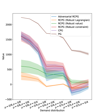
(a) Test value

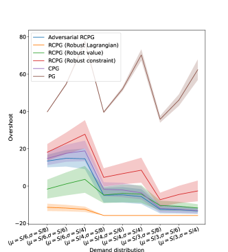
(b) Test overshoot

Figure 1: Test performance metrics of the algorithms on the test set of perturbed transition dynamics in Inventory Management. For each of 20 training runs, each parameter setting is run 50 times and the plot displays the mean and standard error over runs. The parameter manipulated is the mean, $\mu$, and standard deviation, $\sigma$, of the demand distribution.

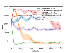
(a) Training value

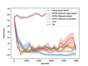
(b) Training overshoot

Figure 5: Training performance metrics of the algorithms over 5,000 episodes on Inventory Management. Note that training performance corresponds to the performance on the simulated transition dynamics, which is defined differently for the different algorithms.

The model estimation phase is based on 100 episodes with $\mu=S/4$ and $\sigma=S/6$, yielding uncertainty sets with budget $\alpha$ ranging in $[0.3,0.9]$ across the state-action space. The policy training phase consists of 5,000 episodes. The widely varying values and overshoots during training (see Figure 5) reflect in part a different training environment. Oscillating behaviours shown by RCPG algorithms are attributed to large abrupt changes in the estimated worst-case distribution. The policy test phase consists of 9 different demand distributions based on $\mu\in\{S/6,S/4,S/3\}$ and $\sigma\in\{S/8,S/6,S/4\}$, each of which are run 50 times. Note that while $\mu$ and $\sigma$ change the demand distribution, the purchasing limit is still based on a mean of $S/4$ and a standard deviation of $S/6$; in other words, the transition dynamics change but the constraint-cost function does not. The penalised return scores in Table  1 demonstrates that RCPG (Robust Lagrangian) has the highest penalised return. This indicates that robustifying the Lagrangian is beneficial but also that the abrupt changes in the estimated worst-case distribution do not appear to hamper RCPG’s test performance; a further analysis of this observation is found in Section 6.3.

6.2 Safe Navigation

The second domain and third domain are safe navigation tasks in a 5-by-5 square grid world, formulated specifically to highlight the advantages of agents that satisfy constraints robustly (see Figure 2). The objective is to move from start, $s_{0}=(0,0)$ to goal, $(4,4)$, as quickly as possible while avoiding areas that incur constraint-costs. The agent observes its $(x,y)$-coordinate and outputs an action going one step left, one step right, one step up, or one step down. The episode is terminated if either the agent arrives at the goal square or if more than $T$ time steps have passed. Instead of using the full state space as next states in the uncertainty sets, the probability vectors $\mathcal{P}_{s,a}$ consider for the next state only the 5 states in the Von Neumann neighbourhood $\mathcal{N}(s)$ with Manhattan distance of at most 1 from $s$; this requires setting $\alpha(s,a)=\sqrt{\frac{2}{n(s,a)}\ln\left(\frac{2^{S^{\prime}}SA}{\delta}\right)}$, replacing $S$ by $S^{\prime}=5$ in the set of outcomes.

(a) Save Navigation 1

(b) Safe Navigation 2

Figure 2: Illustration of the safe navigation tasks. In Safe Navigation 1, the constraint is to hit no more than 4 grey cells on average. In Safe Navigation 2, the constraint is to avoid the red cells and only a limited number of grey cells. In both tasks, unconstrained solutions (red) will go to the goal as quick as possible regardless of the cost incurred; constrained solutions (orange) avoid the costs as far as it is need to satisfy the budget; and robust-constrained solutions (green) take a path that maintains a distance from cells to avoid high cost in perturbed dynamics. The arrows represent the worst-case transitions for test Safe Navigation 2B.

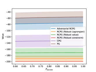
(a) Test A value

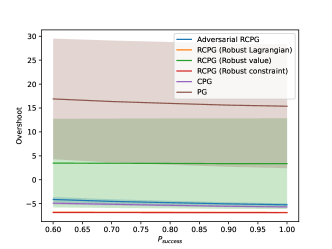
(b) Test A overshoot

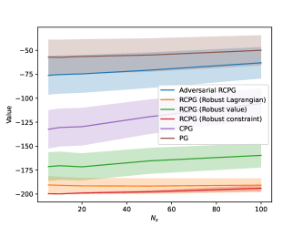
(c) Test B value

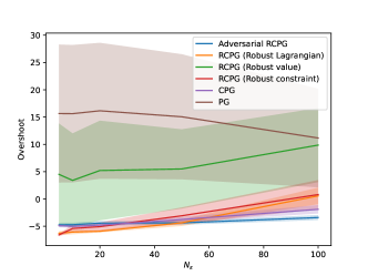
(d) Test B overshoot

Figure 3: Test performance metrics of the algorithms on the test set of perturbed transition dynamics in Safe Navigation 1. For each of 20 training runs, each parameter setting is run 50 times and the plot displays the mean and standard error over runs. Test A: The parameter manipulated is the success probability of the actions, $P_{\text{success}}\in\{0.60,0.70,0.8,0.9,1.0\}$. Test B: The parameter manipulated is the number of perturbations, $N_{\epsilon}\in\{5,10,20,50,100\}$, which represents the number of randomly selected state-action pairs that are perturbed with a random offset in $\mathcal{N}(s)$.

Safe Navigation 1

In Safe Navigation 1 (see Figure 2a), the grid contains 6 grey cells that incur constraint-cost of $1.0$ and agents should satisfy a budget of $d=3.0$. Agents stay in the grid world for $T=200$ time steps if the goal is not found. The model estimation phase is based on 100 episodes, which results in the uncertainty budget $\alpha$ ranging in $[0.25,0.7]$ across the state-action space. In this phase, the success probability is set to $P_{\text{success}}=0.80$, which indicates that the action in a state $s$ succeeds with probability $P_{\text{success}}$ and with probability $1-P_{\text{success}}$ the agent stands still. The training phase consists of 5,000 episodes of training, resulting in uncertainty. The test phase runs two separate tests. Test 1A manipulates $P_{\text{success}}\in\{0.60,0.70,0.80,0.90,1.0\}$. Test 1B keeps $P_{\text{success}}=0.80$ but injects state-action specific perturbations $\epsilon(s,a)\sim\mathcal{N}(s)$ such that with probability $P_{\text{success}}$ the agent successfully moves to the desired location but with probability $1-P_{\text{success}}$ the agent is transported to $s+\epsilon(s,a)$. The number of state-action pairs perturbed is manipulated as $N_{\epsilon}\in\{5,10,20,50,100\}$.

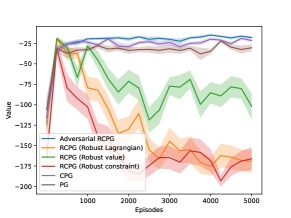
(a) Training value

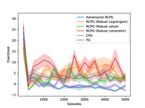
(b) Training overshoot

Figure 6: Training performance metrics of the algorithms over 5,000 episodes on Safe Navigation 1. Note that training performance corresponds to the performance on the simulated transition dynamics, which is defined differently for the different algorithms.

As shown in Table 1, Adversarial RCPG outperforms all other algorithms in both tests of Safe Navigation 1. In line with the hypothesis that Adversarial RCPG provides incremental learning, Figure 6 in Appendix A shows that the training value and constraint-overshoot develop much more smoothly in Adversarial RCPG when compared to RCPG variants, which display oscillating and high-variance scores on these metrics. In the test, the RCPG algorithms do not find paths to the goal location although the RCPG (Robust constraint) and RCPG (Robust Lagrangian) satisfy the constraint. As shown in Figure 3, Adversarial RCPG combines a high value comparable to PG with a negative overshoot that is not affected even by severe perturbations.

Safe Navigation 2

In Safe Navigation 2 (see Figure 2b), the grid contains 7 grey cells that incur constraint-cost of $0.1$, 4 red cells that incur a cost of $1.0$, and agents should satisfy a budget of $d=0.4$. Agents stay in the grid world for $T=100$ time steps if the goal is not found. The data collection phase is based on 10000 episodes with $P_{\text{success}}=1.0$. The resulting uncertainty set has a smaller uncertainty budget, with $\alpha$ ranging in $[0.03,0.085]$ across the state-action space. The training phase consists of 5,000 episodes of training based on the uncertainty set (see Appendix A for details and performance plots). There are two distinct tests. Test 2A manipulates $P_{\text{success}}\in\{0.60,0.70,0.80,0.90,1.0\}$, where the failure makes the agent stands still. Test 2B keeps $P_{\text{success}}=0.80$ but rather than standing still, the agent is moved according to worst-case transitions as shown in the arrows of Figure 2b.

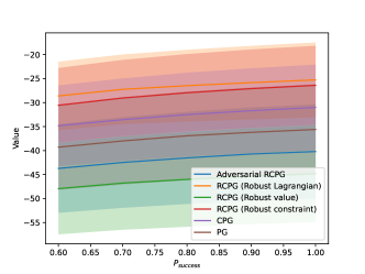
(a) Test A value

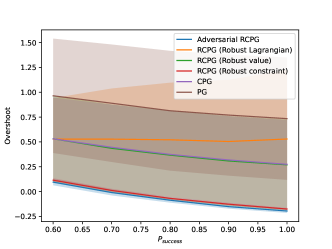
(b) Test A overshoot

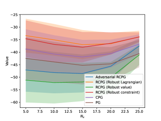
(c) Test B value

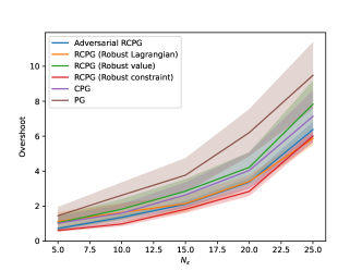
(d) Test B overshoot

Figure 4: Test performance metrics of the algorithms on the test set of perturbed transition dynamics in Safe Navigation 2. For each of 20 training runs, each parameter setting is run 50 times and the plot displays the mean and standard error over runs. Test A: The parameter manipulated is the success probability of the actions, $P_{\text{success}}\in\{0.60,0.70,0.8,0.9,1.0\}$. Test B: The parameter manipulated is the number of perturbations, $N_{\epsilon}\in\{5,10,15,20,25\}$, which represents the number of randomly selected states that are perturbed with a worst-case transition according to the arrows in Figure 2b.

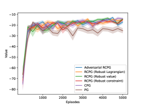
(a) Training value

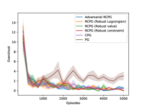
(b) Training overshoot

Figure 7: Training performance metrics of the algorithms over 5,000 episodes on Safe Navigation 2. Note that training performance corresponds to the performance on the simulated transition dynamics, which is defined differently for the different algorithms.

As shown in Table 1, RCPG (Robust constraint) is the top performer followed by Adversarial RCPG in both tests of Safe Navigation 2. Figure 7 in Appendix A shows that the training value and constraint-overshoot now are equally smooth when comparing RCPG variants to Adversarial RCPG. The discrepancy between Safe Navigation 2 and Safe Navigation 1 is attributed to two factors, namely the difference between the worst case and the average case being reduced due to the lower maximal number of time steps $T=100$ (compared to $T=200$ in Safe Navigation 1) as well as the more narrow uncertainty set formed from $N=10,000$ (compared to $N=100$ in Safe Navigation 1). In this case, the performance of RCPG (Robust Lagrangian) is also comparable to Adversarial RCPG, which is consistent with the explanation that RCPG does not experience the incremental learning issue in this domain. Robustifying the constraint only may be beneficial in this domain due to the constraint-cost dynamics being much more challenging than finding paths towards goal. As shown in Figure 4, Adversarial RCPG does not have the highest value but achieves a low overshoot comparable to RCPG (Robust constraint). RCPG (Robust Lagrangian) also performs comparably on the overshoot on test B.

6.3 Analysis

While RCPG displays abrupt changes in the training performance as a consequence of sudden changes in the worst-case transition dynamics, Adversarial RCPG displays smooth incremental learning. This is attributed to starting from the nominal and making gradual changes in the transition dynamics rather than oscillating between highly differing distributions found by linear programming on a changing sorted value list. As observed in the experiments, how well this translates into improved vs reduced test performance differs across domains. Safe Navigation 1 presents a particular challenge for RCPG; this is attributed to learning paths that satisfy the constraint (by avoiding grey cells) but that do not come closer to the goal. By contrast, the Adversarial RCPG starts from the nominal model, which helps to consolidate some initial paths before moving on to more challenging dynamics. In Inventory Management, there are limited sequential dependencies because any state is reachable from any other state and the demand is iid; this makes the problem less sensitive to excessive sampling of a single state and shifting transition dynamics. For Safe Navigation 2, the risk of getting stuck is more limited due to the narrower uncertainty set and shorter time horizon.

7 Conclusion and future work

Providing robustness as well as constraints into policies is of critical importance for safe reinforcement learning. Robust Constrained Policy Gradient (RCPG) is a previously proposed algorithm for Robust-constrained Markov decision processes (RCMDPs), a theoretically sound framework for constrained reinforcement learning with robustness to model uncertainty. This paper proposes modifications to RCPG by robustifying the full constrained objective through a robust Lagrangian objective and improving incremental learning through an adversarial policy gradient. These modifications are empirically demonstrated to improve reward-based and constraint-based metrics on a wide range of test perturbations. Adversarial policies have been of interest in designing realistic attacks on reinforcement learning policies (e.g. [26, 27]); while these works do not consider uncertainty sets, an interesting avenue for future research is to extend Adversarial RCPG with uncertainty sets that satisfy realism constraints in addition to the current norm constraints.

Appendix A: Proof of Robust Constrained Policy Gradient theorem

Using the notation $\mathbf{r}(s,a)=r(s,a)-\lambda c(s,a)$ to formulate the problem as an MDP, we have

$$\nabla_{\theta} \mathbf{V}_{\pi}(s)=\nabla_{\theta}\sum_{a\in\mathcal{A}}\pi(a|s)\mathbf{Q}_{\pi}(s,a)$$

$$=\sum_{a\in\mathcal{A}}\mathbf{Q}_{\pi}(s,a)\nabla_{\theta}\pi(a|s)+\pi(a|s)\nabla_{\theta}\mathbf{Q}_{\pi}(s,a)\quad\quad\text{(product rule)}$$

$$=\sum_{a\in\mathcal{A}}\mathbf{Q}_{\pi}(s,a)\nabla_{\theta}\pi(a|s)+\pi(a|s)\quad\quad\quad\nabla_{\theta}\sum_{s^{\prime},\mathbf{r}}\mathbb{P}(s^{\prime},\mathbf{r}|a,s)\left(\mathbf{r}(s,a)+\mathbf{V}_{\pi}(s^{\prime})\right)\quad\quad\text{(bootstrap from next Q)}$$

$$=\sum_{a\in\mathcal{A}}\mathbf{Q}_{\pi}(s,a)\nabla_{\theta}\pi(a|s)+\pi(a|s)\nabla_{\theta}\sum_{s^{\prime}}P(s^{\prime}|a,s)\nabla_{\theta}\mathbf{V}_{\pi}(s^{\prime})\quad\quad\text{(noting that ($P(s^{\prime}|a,s)=\sum_{r}\mathbb{P}(s^{\prime},\mathbf{r}|a,s)$)}$$

$$=\sum_{a\in\mathcal{A}}\mathbf{Q}_{\pi}(s,a)\nabla_{\theta}\pi(a|s)+\pi(a|s)\sum_{s^{\prime}}P(s^{\prime}|s,a)\left(\sum_{a^{\prime}\in\mathcal{A}}\nabla_{\theta}\pi(a^{\prime}|s^{\prime})\mathbf{Q}_{\pi}(s^{\prime},a^{\prime})+\pi(a^{\prime}|s^{\prime})\sum_{s^{\prime\prime}}P(s^{\prime\prime}|s^{\prime},a^{\prime})\nabla_{\theta}\mathbf{V}_{\pi}(s^{\prime\prime})\right)$$

(unpacking analogously)

$$=\sum_{s_{\text{next}}\in\mathcal{S}}\sum_{k=0}^{\infty}\mathbb{P}(s\to s_{\text{next}}|k,\pi)\sum_{a}\mathbf{Q}_{\pi}(s,a)\nabla_{\theta}\pi(a|s)\quad\quad\text{(repeated unpacking)}$$

To demonstrate the objective is satisfied from $t=0$ to $t=\infty$, the proof continues from the initial state $s_{0}$. There it is useful to consider the average number of visitations of $s$ in an episode, $n(s):=\sum_{k=0}^{\infty}\mathbb{P}(s_{0}\to s|k,\pi)$, and its relation to the on-policy distribution $\mu(s|\pi)$, the fraction of time spent in each state when taking actions from $\pi$:

$$\nabla_{\theta}\mathbf{V}_{\pi}(s_{0}) =\sum_{s\in\mathcal{S}}n(s)\sum_{a}\mathbf{Q}_{\pi}(s,a)\nabla_{\theta}\pi(a|s)$$

$$=\sum_{s\in\mathcal{S}}n(s)\sum_{a}\mathbf{Q}_{\pi}(s,a)\nabla_{\theta}\pi(a|s)$$

$$\propto\sum_{s\in\mathcal{S}}\mu(s|\pi)\sum_{a}\mathbf{Q}_{\pi}(s,a)\nabla_{\theta}\pi(a|s)$$

$$=\mathbb{E}_{\pi,P}\left[\sum_{a}\nabla_{\theta}\mathbf{Q}_{\pi}(s_{t},a)\pi(a|s_{t})\right]$$

$$=\mathbb{E}_{\pi,P}\left[\sum_{a}\mathbf{Q}_{\pi}(s_{t},a)\pi(a|s_{t})\frac{\nabla_{\theta}\pi(a|s_{t})}{\pi(a|s_{t})}\right]$$

$$=\mathbb{E}_{\pi,P}\left[\frac{\mathbf{Q}_{\pi}(s_{t},a_{t})\nabla_{\theta}\pi(a_{t}|s_{t})}{\pi(a_{t}|s_{t})}\right]$$

$$=\mathbb{E}_{\pi,P}\left[\mathbf{Q}_{\pi}(s_{t},a_{t})\nabla_{\theta}\log\left(\pi(a_{t}|s_{t})\right)\right]\,.$$

∎

Appendix B: proof of Robust Constrained Adversarial Policy Gradient Theorem

First note that the gradient of $\mathbf{V}_{\pi}(s_{t})$ of a state $s_{t}$ at time $t$ is given by

$$\nabla_{\theta_{\text{adv}}} \mathbf{V}_{\pi}(s_{t})=\nabla_{\theta_{\text{adv}}}\left(\sum_{a}\pi(a|s_{t})\mathbf{Q}_{\pi}(s_{t},a)\right)$$

$$=\sum_{a}\pi(a|s_{t})\nabla_{\theta_{\text{adv}}}\mathbf{Q}_{\pi}(s_{t},a)\quad\quad\text{($\pi$ independent of $\pi_{\text{adv}}$ )}$$

$$=\sum_{a}\pi(a|s_{t})\nabla_{\theta_{\text{adv}}}\left(\mathbb{P}(s^{\prime},\mathbf{r}|s_{t},a)\left(\sum_{\mathbf{r},s^{\prime}}\mathbf{r}(s_{t},a)+\mathbf{V}_{\pi}(s^{\prime})\right)\right)\quad\quad\text{(expand the Q-value)}$$

$$=\sum_{a}\pi(a|s_{t})\quad\quad\quad\nabla_{\theta_{\text{adv}}}\left(\sum_{s^{\prime}}\mathbb{P}(s^{\prime}|s_{t},a)\mathbf{V}_{\pi}(s^{\prime})\right)\quad\quad\text{(reward distribution independent of $\pi_{\text{adv}}$)}$$

$$=\sum_{a}\pi(a|s_{t})\nabla_{\theta_{\text{adv}}}\left(\sum_{s^{\prime}}\pi_{\text{adv}}(s^{\prime}|s_{t},a)\mathbf{V}_{\pi}(s^{\prime})\right)\quad\quad\text{(use $\pi_{\text{adv}}$ to generate the next state)}$$

$$=\sum_{a}\pi(a|s_{t})\left(\sum_{s^{\prime}}\mathbf{V}_{\pi}(s^{\prime})\nabla_{\theta_{\text{adv}}}\pi_{\text{adv}}(s^{\prime}|s_{t},a)+\pi_{\text{adv}}(s^{\prime}|s_{t},a)\nabla_{\theta_{\text{adv}}}\mathbf{V}_{\pi}(s^{\prime})\right)\quad\quad\text{(product rule)}$$

$$=\sum_{a}\pi(a|s_{t})\left(\sum_{s^{\prime}}\mathbf{V}_{\pi}(s^{\prime})\pi_{\text{adv}}(s^{\prime}|s_{t},a)\frac{\nabla_{\theta_{\text{adv}}}\pi_{\text{adv}}(s^{\prime}|s_{t},a)}{\pi_{\text{adv}}(s^{\prime}|s_{t},a)}+\nabla_{\theta_{\text{adv}}}\mathbf{V}_{\pi}(s^{\prime})\right)\quad\quad\text{(divide and multiply by $\pi_{\text{adv}}$)}$$

$$=\mathbb{E}_{\pi,\pi_{\text{adv}}}\left[\mathbf{V}_{\pi}(s_{t+1})\frac{\nabla_{\theta_{\text{adv}}}\pi_{\text{adv}}(s_{t+1}|s_{t},a_{t})}{\pi_{\text{adv}}(s_{t+1}|s_{t},a_{t})}+\nabla_{\theta_{\text{adv}}}\mathbf{V}_{\pi}(s_{t+1})\right]\quad\quad\text{(expectation over $\pi$ and $\pi_{\text{adv}}$ )}$$

$$=\mathbb{E}_{\pi,\pi_{\text{adv}}}\left[\mathbf{V}_{\pi}(s_{t+1})\nabla_{\theta_{\text{adv}}}\log\left(\pi_{\text{adv}}(s_{t+1}|s_{t},a_{t})\right)+\nabla_{\theta_{\text{adv}}}\mathbf{V}_{\pi}(s_{t+1})\right]\,.\quad\quad\text{(derivative of logarithm)}$$

Therefore, expanding this sum across all times $t=0,\dots,H$, were $H$ is the horizon of the decision process, the expression for $t=0$ is given by

$$\nabla_{\theta_{\text{adv}}}\mathbf{V}_{\pi}(s_{0}) =\sum_{k=1}^{H}\mathbb{E}_{\pi,\pi_{\text{adv}}}\left[\mathbf{V}_{\pi}(s_{k+1})\log\left(\pi_{\text{adv}}(s_{t+1}|s_{t},a_{t})\right)\right]\,.$$

∎

Appendix C: Training hyperparameters and analysis

Hyperparameters

Hyperparameters are set according to Table 2. The discount is common at 0.99 and the architecture was chosen such that it is large enough for both domains. The entropy regularisation is higher than usual training procedures because of the Lagrangian yielding larger numbers in the objective. Learning rates were tuned in $\{0.10,0.01,0.001\}$ for policy parameters ($\theta$ and $\theta_{\text{adv}}$) and in $\{0.01,0.001,0.0001\}$ for Lagrangian multipliers ($\lambda$ and $\lambda_{\text{adv}}$); the setting shown in the table is the best setting for Inventory Management and Safe Navigation domains and this loosely corresponds to the two time scale stochastic approximation criteria [28]. The critic was fixed to 0.001 for both domains as this is a reliable setting for the Adam optimiser. For Inventory Management, it is possible to satisfy the constraint from the initial stages of learning so the initial Lagrangian multiplier $\lambda$ is set to 50. For Safe Navigation domains, the initial $\lambda$ is set to 1 since it is not immediately possible to satisfy the constraints without learning viable paths to goal.

Table 2: Parameter settings of the experiments

Parameter	Setting
Discount	0.99
Entropy regularisation for $\pi$	5.0
Architecture for $\pi$ and $\pi_{\text{adv}}$	100 hidden RELU units, softmax output
Learning rates for $\theta$,$\lambda$,$\theta_{\text{adv}}$, and $\lambda_{\text{adv}}$	0.001, 0.0001, 0.001, and 0.0001, multiplier $\frac{1}{1+n//500}$ for episode $n$
Initialisation of $\lambda$ and $\lambda_{adv}$	both 50 for Inventory Management, both 1 for Safe Navigation 1 & 2
Critic	learning rate 0.001, 100 hidden RELU units, linear output, Adam optimisation of MSE, batch is episode

Training performance plots

References

- [1] E. Altman, Constrained Markov decision processes. Chapman and Hall/CRC, 1998.
- [2] S. Gu, L. Yang, Y. Du, G. Chen, F. Walter, J. Wang, Y. Yang, and A. Knoll, “A Review of Safe Reinforcement Learning: Methods, Theory and Applications,” arXiv preprint, 2022.
- [3] G. N. Iyengar, “Robust dynamic programming,” Mathematics of Operations Research, vol. 30, no. 2, pp. 257–280, 2005.
- [4] A. Nilim and L. E. Ghaoui, “Robust control of Markov decision processes with uncertain transition matrices,” Operations Research, vol. 53, no. 5, pp. 780–798, 2005.
- [5] J. Van Baar, A. Sullivan, R. Cordorel, D. Jha, D. Romeres, and D. Nikovski, “Sim-to-real transfer learning using robustified controllers in robotic tasks involving complex dynamics,” in Proceedings of the IEEE International Conference on Robotics and Automation (ICRA 2019), pp. 6001–6007, 2019.
- [6] C. Finn, P. Abbeel, and S. Levine, “Model-Agnostic Meta-Learning for Fast Adaptation of Deep Networks,” in Proceedings of the International Conference on Machine Learning (ICML 2017), (Sydney, Australia), 2017.
- [7] R. H. Russel, M. Benosman, and J. Van Baar, “Robust Constrained-MDPs: Soft-Constrained Robust Policy Optimization under Model Uncertainty,” arXiv preprint, 2020.
- [8] R. H. Russel, M. Benosman, J. van Baar, and R. Corcodel, “Lyapunov Robust Constrained-MDPs for Sim2Real Transfer Learning,” in Federated and Transfer Learning, vol. 27, pp. 307–328, 2022.
- [9] D. P. Bertsekas, Nonlinear programming. Athena Scientific, 2003.
- [10] J. Achiam, D. Held, A. Tamar, and P. Abbeel, “Constrained policy optimization,” in Proceedings of the International Conference on Machine Learning (ICML 2017), vol. 1, pp. 30–47, 2017.
- [11] A. Ray, J. Achiam, and D. Amodei, “Benchmarking Safe Exploration in Deep Reinforcement Learning,” arXiv preprint, pp. 1–6, 2019.
- [12] M. Petrik, “RAAM : The Benefits of Robustness in Approximating Aggregated MDPs in Reinforcement Learning,” in Advances in Neural Information Processing Systems (NeurIPS 2005), pp. 1–9, 2005.
- [13] D. M. Bossens and N. Bishop, “Explicit Explore, Exploit, or Escape (): near-optimal safety-constrained reinforcement learning in polynomial time,” Machine Learning, 2022.
- [14] D. J. Mankowitz, D. A. Calian, R. Jeong, C. Paduraru, N. Heess, S. Dathathri, M. Riedmiller, and T. Mann, “Robust Constrained Reinforcement Learning for Continuous Control with Model Misspecification,” arXiv preprint, pp. 1–23, 2020.
- [15] L. Zheng and L. J. Ratliff, “Constrained Upper Confidence Reinforcement Learning with Known Dynamics,” in Proceedings of the Annual Conference on Learning for Dynamics and Control (L4DC 2020), pp. 1–10, 2020.
- [16] Y. Chow and M. Ghavamzadeh, “Algorithms for CVaR optimization in MDPs,” in Advances in Neural Information Processing Systems (NeurIPS 2014), pp. 3509–3517, 2014.
- [17] Q. Yang, T. D. Simão, S. H. Tindemans, and M. T. J. Spaan, “WCSAC: Worst-Case Soft Actor Critic for Safety-Constrained Reinforcement Learning,” in Proceedings of the Association for the Advancement of Artificial Intelligence (AAAI 2021), vol. 35, pp. 10639–10646, 2021.
- [18] R. Zhang and J. Sjölund, “Risk-sensitive Actor-free Policy via Convex Optimization,” in AISafety and SafeRL Joint Workshop at the International Joint Conference on Artificial Intelligence (IJCAI 2023), 2023.
- [19] Y. Chow, O. Nachum, A. Faust, E. Duenez-Guzman, and M. Ghavamzadeh, “Lyapunov-based Safe Policy Optimization for Continuous Control,” in Proceedings of the Reinforcement Learning for Real Life Workshop in the International Conference on Machine Learning (ICML 2019), 2019.
- [20] R. Laroche, P. Trichelair, and R. T. Des Combes, “Safe policy improvement with baseline bootstrapping,” in Proceedings of the International Conference on Machine Learning (ICML 2019), pp. 6487–6520, 2019.
- [21] H. Satija, J. Pineau, P. S. Thomas, and R. Laroche, “Multi-Objective SPIBB: Seldonian Offline Policy Improvement with Safety Constraints in Finite MDPs,” in Advances in Neural Information Processing Systems (NeurIPS 2021), pp. 2004–2017, 2021.
- [22] R. H. Russel and M. Petrik, “Beyond confidence regions: Tight Bayesian ambiguity sets for robust MDPs,” in Advances in Neural Information Processing Systems (NeurIPS 2019), vol. 32, 2019.
- [23] M. A. Taleghan and T. G. Dietterich, “Efficient exploration for constrained MDPs,” in AAAI Spring Symposium – Technical Report, pp. 313–319, 2018.
- [24] R. S. Sutton and A. G. Barto, Reinforcement Learning: An Introduction. MIT Press, second edition ed., 2017.
- [25] Puterman, Martin L, Markov Decision Processes: Discrete Stochastic Dynamic Programming. Wiley New York, 2005.
- [26] A. Gleave, M. Dennis, C. Wild, N. Kant, S. Levine, and S. Russell, “Adversarial Policies: Attacking Deep Reinforcement Learning,” in Proceedings of the International Conference on Learning Representations (ICLR 2020), pp. 1–16, 2020.
- [27] A. Mandlekar, Y. Zhu, A. Garg, L. Fei-Fei, and S. Savarese, “Adversarially Robust Policy Learning: Active construction of physically-plausible perturbations,” in IEEE International Conference on Intelligent Robots and Systems, pp. 3932–3939, 2017.
- [28] V. S. Borkar, Stochastic Approximation: A Dynamical Systems Viewpoint. Springer, second ed., 2022.