Superdeterminism Without Conspiracy
Abstract
Superdeterminism - where the Measurement Independence assumption in Bell’s Theorem is violated - is frequently assumed to imply implausibly conspiratorial correlations between properties of particles being measured and measurement settings and . But it doesn’t have to be: a superdeterministic but non-conspiratorial locally causal model is developed where each pair of entangled particles has unique . The model is based on a specific but arbitrarily fine discretisation of complex Hilbert space, where defines the information, over and above the freely chosen nominal settings and , which fixes the exact measurement settings and of a run of a Bell experiment. Pearlean interventions, needed to assess whether and are Bell-type free variables, are shown to be inconsistent with rational-number constraints on the discretised Hilbert states. These constraints limit the post-hoc freedom to vary keeping and fixed but disappear with any coarse-graining of , and , rendering so-called drug-trial conspiracies irrelevant. Points in the discretised space can be realised as ensembles of symbolically labelled deterministic trajectories on an ‘all-at-once’ fractal attractor. It is shown how quantum mechanics might be ‘gloriously explained and derived’ as the singular continuum limit of the discretisation of Hilbert space; It is argued that the real message behind Bell’s Theorem has less to do with locality, realism or freedom to choose, and more to do with the need to develop more explicitly holistic theories when attempting to synthesise quantum and gravitational physics.
1 Introduction
A deterministic hidden-variable model is said to be superdeterministic - not a word the author would have chosen - if the so-called Measurement Independence assumption (sometimes referred to as the Statistical Independence assumption or the -independence assumption),
| (1) |
is violated [19] [44] [14] [22] [47]. Here is a probability density on a set of hidden variables , and and denote experimentally chosen measurement settings - for concreteness, nominally accurate polariser orientations. Without (1), it is impossible to show that model satisfies the CHSH version of Bell’s inequality
| (2) |
where denotes a correlation on Bell-experiment measurement outcomes over an ensemble of particle pairs prepared in the singlet state.
The argument that models which violate (1) are conspiratorial, originates in a paper by Shimony, Horne and Clauser, written in response to Bell’s paper on local beables [7]. Shimony et al write:
In any scientific experiment in which two or more variables are supposed to be randomly selected, one can always conjecture that some factor in the overlap of the backwards light cones has controlled the presumably random choices. But, we maintain, skepticism of this sort will essentially dismiss all results of scientific experimentation. Unless we proceed under the assumption that hidden conspiracies of this sort do not occur, we have abandoned in advance the whole enterprise of discovering the laws of nature by experimentation.
The drug trial is often used to illustrate the contrived nature of such a conspiracy. For example [18]:
if you are performing a drug versus placebo clinical trial, then you have to select some group of patients to get the drug and some group of patients to get the placebo. The conclusions drawn from the study will necessarily depend on the assumption that the method of selection is independent of whatever characteristics those patients might have that might influence how they react to the drug.
Related to this, superdeterminism is sometimes described as requiring exquisitely (and hence unrealistically) finely tuned initial conditions [4], or as negating experimenter freedom [51]. A number of quantum foundations experts (e.g. [29] [49] [3] [1]) use one or more of these arguments to dismiss superdeterminism in derisive terms.
A new twist was added by Aaronson [1] who concluded his excoriating critique of superdeterminism with a challenge:
Maxwell’s equations were a clue to special relativity. The Hamiltonian and Lagrangian formulations of classical mechanics were clues to quantum mechanics. When has a great theory in physics ever been grudgingly accommodated by its successor theory in a horrifyingly ad-hoc way, rather than gloriously explained and derived?
It would seem that developing superdetermistic models of quantum physics is a hopeless cause. However, the purpose of this paper is to attempt to show that superdeterminism has been badly misunderstood, to rebuff these criticisms and indeed suggest that violating (1) is perhaps the only sensible way to understand the experimental violation of Bell inequalities. Importantly, we show that whilst conspiracy would imply a violation of (1), the converse is not true. In Section 2, we define what we mean by a non-conspiratorial violation of (1) and how it differs from these more traditional conspiratorial violations. Motivated by this, and the unshieldable effects of gravity as described in Section 3, a non-conspiratorial superdeterministic model is described in Section 4, based on a specific discretisation of complex Hilbert Space [35]. Using the homeomorphism between -adic integers and fractal geometry, the model is linked to the invariant set postulate [33] - the universe is evolving precisely on some special dynamically invariant subset of state space. In Section 5 it is shown how this model violates (1) non-conspiratorially, and indeed violates (2) in exactly the same way as does quantum mechanics. In Section 5.3 we show that the superdeterministic model is locally causal. In Section 6 we discuss common objections to superdeterminism including fine tuning, free will and the so-called drug-trial analogy. Addressing Aaronson’s challenge in Section 6.3, we show how the state space of quantum mechanics can be considered the singular continuum limit of the discretised Hilbert space of the superdeterministic model. A possible experimental test of the supderdeterministic model is discussed in Section 7.
Before embarking on this venture, one may ask answer the question: why bother? After all, quantum mechanics is an extremely well tested theory, and has never been found wanting. Why not just accept that quantum theory violates the concept of local realism - whatever that means - and get on with it? The author’s principal motivation for pursuing theories of physics which violate (1) lies in the possibility of finding a theory of quantum physics that is not inconsistent with the locally causal nonlinear geometric determinism of general relativity theory. As discussed in Section 8, results from this paper suggest that instead of seeking a quantum theory of gravity (‘quantum gravity’) we should be seeking a strongly holistic gravitational theory of the quantum, from which the Euclidean geometry of space-time is emergent as a coarse-grained approximation to the -adic geometry of state space. This, the author believes, is the real message behind the experimental violation of Bell inequalities.
2 Conspiratorial and Non-conspiratorial Interventions
There is no doubt that conspiratorial violations of Bell inequalities, of the type mentioned in the Introduction, imply a violation of (1). Here we are concerned with the converse question: does a violation of (1) imply the existence of a conspiratorial hidden variable theory? In preparing to answer this question, we quote from Bell’s response ‘Free Variables and Local Causality’ [7] (FVLC) to Shimony et al [7]. In FVLC, Bell writes:
I would insist here on the distinction between analyzing various physical theories, on the one hand, and philosophising about the unique real world on the other hand. In this matter of causality it is a great inconvenience that the real world is given to us once only. We cannot know what would have happened if something had been different. We cannot repeat an experiment changing just one variable; the hands of the clock will have moved and the moons of Jupiter. Physical theories are more amenable in this respect. We can calculate the consequences of changing free elements in a theory, be they only initial conditions, and so can explore the causal structure of the theory. I insist that B [Bell’s paper on the theory of local beables [7]] is primarily an analysis of certain kinds of physical theory.
To understand the significance of this quote, we base the analysis of this paper around the thought experiment devised by Bell in FVLC, where, by design, human free will plays no explicit role. Bell supposes and are determined by the outputs of two pseudo-random number generators (PRNGs). These outputs are sensitive to the parity and of the millionth digits of the PRNG inputs. Bell now makes what he calls a ‘reasonable’ assumption:
But this peculiar piece of information [whether the parity of the millionth digit is odd or even] is unlikely to be the vital piece for any distinctively different purpose, i.e., it is otherwise rather useless In this sense the output of such a [PRNG] device is indeed a sufficiently free variable for the purpose at hand.
It is important to note that, in this quote, Bell deflects discussion away from statistical properties of some ensemble of runs of an experiment where measurement settings are supposedly selected randomly (as per the Shimony et al quote above), and focusses on one individual run of an experiment. There is an important reason for this. When discussing conspiratorial hidden-variable models of the Shimony et al type, it is assumed that in any large enough ensemble with common value of , there exist sub-ensembles for each of the four pairs of measurement settings (, , and ). In this context, (1) implies that the four sub-ensembles are statistically equal. Conversely, in a conspiratorial violation of (1), the four sub-ensembles are statistically unequal. In such a situation, can be interpreted as a frequency of occurrence within each of the four sub-ensembles. It is worth noting that in such a frequency-based interpretation of , the issue of counterfactual definiteness - a central issue below - never arises. This has led to a misconception that counterfactual definiteness plays no role in Bell’s Theorem.
Importantly, hidden-variable models do not have to be like this. It is possible that the value of is unique to each run of a Bell experiment. The model described below has this property. In this situation, if were to define a frequency of occurrence, and a particle with value was measured with settings and and could only be measured once, then and where and . However, this does not itself imply a violation of (1) - it merely emphasises that is fundamentally not a frequency of occurrence in an ensemble but rather is a probability density defined on an individual particle with value .
With that in mind, let us continue to focus, as Bell does, on a single entangled particle pair. If and were not free variables, then or would not be vital for ’distinctively different’ purposes. That is to say, we could vary or without having a vital impact on distinctly different systems. In the language of Pearl’s causal inference theory [38], if and were not free variables, there would exist small so-called interventions which by design changed or , and by consequence had a vital impact on distinctly different systems.
The most important part of this paper is to draw attention to two possible ways this might happen. The first is the conventional way where the effect of the intervention propagates causally from its localised source in space-time, somehow vitally influencing distinctly different systems. It is hard to imagine how varying something as insignificant as the parity of the millionth digit of an input to a PRNG could have such a vital impact. For this reason, Bell argued, the PRNG output should indeed be considered a free variable. This, of course, is not unreasonable.
However, there is a second possibility - one that was not considered by Bell - that such interventions are simply inconsistent with physical theory. That is to say, the hypothetical state of the universe where or is perturbed but all other distinctly different elements of the universe are kept fixed, is inconsistent with the laws of physics. If such an intervention was hypothetically applied to a localised region of the universe, the ontological status of the whole universe would change; clearly a state of the universe as a whole only exists if all parts of it satisfy the laws of physics. Of course, we cannot perform an actual experiment to test directly this potential inconsistency: in changing the millionth digit, the hands of the clock and the moons of Jupiter will have moved, as Bell notes. Hence addressing the question of whether the PRNG output is a free variable in the sense of this paragraph requires studying the mathematical properties of physical theory. This is Bell’s point in the first quote and it is the topic of this paper.
Below we develop a model where each particle pair has unique with the property
| (3) |
As will be shown this can be interpreted as a locally causal non-conspiratorial violation of (1). It implies that an intervention on , keeping and fixed, leads to a state of the world which is inconsistent with the model postulates and therefore has zero probability. Clearly, this cannot be an intervention within space-time. Instead the intervention describes a hypothetical perturbation which takes a point in the state space of the universe (labelled by the triple ), consistent with the model and hence with , to a state which is inconsistent with physical theory and hence has . Importantly, this means a non-conspiratorial interpretation of (3) implies that physical theory does not have the post-hoc property of counterfactual definiteness. The essential nature of counterfactuals in Bell’s Theorem was pointed out by Redhead [41] some years ago. This important point seems to have been lost in more recent discussions of Bell’s Theorem.
However, one needs to be careful to not throw the baby out with the bathwater. Counterfactual reasoning is both pervasive and important in physics. Indeed, it is central to the scientific method [28]. The fact that we can express laws of physics mathematically gives us the power to estimate what would have happened had something been different. Such estimates can lead to predictions and the predictions can be verified by experiment. We clearly do not want to give up counterfactual reasoning entirely in our search for new theories of physics. We address this concern by noting that output from experiment and physical theory (particularly when the complexities of the real world are accounted for) involves some inherent coarse-graining. Experiments have some nominal accuracy and output from a computational model is typically truncated to a fixed number of significant digits. We can represent such coarse graining by integrating exact output of physical theory over small volumes in state space, where smoothly as . In developing a superdeterministic model below, we will require that counterfactual definiteness holds generically when variables are coarse grained over volumes , for suitably defined small values . The model based on discretised Hilbert Space, described in Section 4 has this property. As discussed below, this renders the drug-trial analogy irrelevant.
These matters are subtle, and it seems Bell appreciated this. Instead of derisively rejecting theories where (1) is violated he concludes FVLC with the words:
Of course it might be that these reasonable ideas about physical randomisers are just wrong - for the purposes at hand.
Indeed, in his last paper ‘La Nouvelle Cuisine’, Bell writes:
An essential element in the reasoning here is that [polariser settings] are free variables…. Perhaps such a theory could be both locally causal and in agreement with quantum mechanical predictions. However, I do not expect to see a serious theory of this kind. I would expect a serious theory to permit ‘deterministic chaos’ or ‘pseudorandomness’ …But I do not have a theorem about that.
The last sentence is insightful, because, as we discuss, there is no such theorem. Indeed the reverse: here we develop a serious non-classical model where polariser settings are not free variables, utilising geometric concepts in deterministic chaos.
3 The Andromedan Butterfly Effect
The purpose of this section is to note how the Principle of Equivalence makes the interaction of matter with gravity especially chaotic. Here we repeat a calculation first reported by Michael Berry [8] and further analysed in [45]. It is well known that the flap of a butterfly’s wings in Brazil can cause a tornado in Texas. But, could the flap of a butterfly’s wings on a planet in the Andromedan galaxy cause a tornado in Texas?
We consider molecules in the atmosphere as hard spheres of radius with mean free distance between collisions. We wish to estimate the uncertainty in the angle of the th collision of one of the spheres with other spheres, due to some very small uncertain external force. It is easily shown that grows exponentially with . In particular
| (4) |
With and m, . After how many collisions is the position of a molecule in Earth’s atmosphere sensitive to the gravitational uncertainty in the uncertain flap of a butterfly’s wing in the Andromeda galaxy? Let denote the distance between Earth and Andromeda. The flap of a butterfly’s wing through a distance will change the gravitational force on our target molecule by an amount . Uncertainty in the flap of an Andromedan butterfly’s wing will therefore induce an uncertainty in the acceleration of a terrestrial atmospheric molecule by an amount
| (5) |
If denotes the mean time between molecular collisions, there is an uncertainty in the direction of the molecule . Plugging in kg, m, s and m, gives . How large is before ? From the above, . Hence after about 30 collisions the direction the direction of travel of the terrestrial molecule has been rendered completely uncertain by the gravitational effect of the Andromedan butterfly. Indeed one can go further: the direction of the terrestrial molecule is rendered completely uncertain by the uncertain position of a single electron at the edge of the visible universe after about only 50 or so collisions (which below we will round up to an order of magnitude of ). Once the molecules of the Earth’s atmosphere have been disturbed in this way, it is only a matter of a couple of weeks before the nonlinearity of the Navier-Stokes equations leads to uncertainty in a large-scale weather pattern, such as a Texan tornado [27] [36].
Nowhere above did the mass of the molecule enter the calculation. The same calculation could just as well apply to the measurement process in quantum physics - where a particle interacts with atoms in some measuring device. Indeed the same calculation could apply to molecules in an experimenter’s brain, affecting the decisions they make.
As a matter of principle, the direction of motion of a molecule after 100 collisions is for all practical purposes uncomputable. If a computation (say on a supercomputer) was attempted, then the direction of the molecule would depend on the motion of electrons in the chips of the supercomputer. Self-referentially, the computational software would have to include a representation of the computation. Technically, the Andromedan Butterfly Effect describes a computationally irreducible system [50] - one that cannot be computed with a computationally simpler system.
This is the first step in our argument that (1) could be violated because the universe should be considered a rather holistic chaotic system. Gravity is what makes the universe holistic. Unlike the other forces of nature, the effects of gravity cannot be shielded by negative charges. However, by itself, this argument doesn’t imply that the parity of the millionth digit, or the flap of a butterfly’s wings in Andromeda is a vital piece of information for determining distinctly different systems. For that we need more from the theory of chaos.
4 A Superdeterministic Model
4.1 Nominal vs Exact Measurement Settings and Hidden Variables
We build on Bell’s thought experiment whereby polariser orientations are determined by the parities and in Alice and Bob’s PRNGs (supposing there is no particular reason why these would be odd or even). Manifestly, and only determine the polariser orientations to some nominal accuracy. That is, determine small neighbourhoods of the 2-sphere of orientations, referred to as disks. None of the results below depend on the magnitude of as long as (as discussed in Section 6.3, the limit in the proposed model is singular). It will be assumed - consistent with our search for an underlying deterministic theory - that when measurements are made on particular particles, the measurement outcomes are associated with some exact, albeit unknown, polariser orientations and . Here, and denote unit vectors in physical 3-space from the centre of a unit ball, to the surface of the 2-sphere of orientations. The corresponding points on the 2-sphere to which the vectors point are written as and . The nominal directions and refer to unit vectors pointing to the centroids of the disks. In the discussion below, we assume that the probabilistic nature of the quantum measurement problem arises because the measurement outcome is typically sensitive to the exact measurement settings within an disk (c.f. fractally intertwined basins of attraction [32]). Hence, any given nominal setting is consistent with an ensemble of possible exact settings.
With this in mind, we let describe all of the variables which, over and above and , determine the exact measurement settings and . These variables include Andromedan butterflies and electrons at the end of the visible universe. When measuring a single qubit we can frame it like this: consider a spacelike hypersurface in the past of some event where the measurement outcome was known, and before the event where the PRNG output was known, then must include data on , on and inside ’s past light cone, with the exception of (or its determinants). In this way we can write , . The extension of this causal picture for entangled qubits is discussed in Section 5.3.
4.2 Rational Quantum Mechanics: RaQM
Motivated by John Wheeler’s plea to excise the continuum from physical theory [48] - see also [17] - a way to introduce non-conspiratorial superdeterminism into quantum physics is to discretise Hilbert space [11] [12] [35] [13]. At the experimental level this is surely unexceptionable: all experiments which confirm quantum mechanics will necessarily confirm a model of quantum physics based on discretised Hilbert Space, providing the discretisation is fine enough. However, as discussed, such a discretisation has profound implications for the interpretation of quantum experiments
4.2.1 Single Qubits
Consider a qubit prepared in a state , and written as
| (6) |
with respect to some arbitrary basis . We call this a ‘proper basis’ if
| (7) |
where is some large prime number and . In a proper basis, it can be shown [37] that has a representation as a bit string of deterministic elements where equals the fraction of elements in the bit string and denotes a cyclical permutation of elements of the bit string. Here we will assume is a large prime. In RaQM the measurement basis is a proper basis, and the measurement output is a deterministically selected element of the bit string. In this way, each proper basis is a basis with respect to which a measurement could potentially be made by the experimenter. A measurement cannot be made with respect to a basis which is not proper. For each proper basis, the potential measurement outcome is associated with some exact measurement orientation in physical 3-space, which satisfies the rationality constraints
| (8) |
written in base-. In this way, correspond to nominally accurate measurement orientations. In this representation, measurement outcome probabilities (over ensembles of elements of the bit string) automatically satisfy Born’s Rule. Hence Born’s Rule is not a separate axiom in RaQM.
If the exact preparation setting is represented by , and exact measurement setting , then the first of (8) can be written , where denotes the scalar product of two vectors. Because of Niven’s theorem
angles that determine probabilities and angles that determine phases, c.f., (8), are relatively incommensurate, except at the precise values . One can assume that such precise values never occur in practice (any gravitational wave would disturb a system away from such a precise value), though they may be relevant for theoretical reasons (e.g. when one considers a measurement performed with a precisely opposite measurement direction).
An important corollary to Niven’s Theorem - central to this paper - is what we refer to as the Impossible Triangle Corollary:
Corollary.
Let be a triangle on the unit sphere with rational internal angles, not precisely equal to multiples of , such that and . Then .
Proof.
Assume is rational, where denotes the exact angular distance between and on the unit sphere, etc. By the cosine rule for ,
| (9) |
where is the exact internal angle of the triangle at the vertex . Since and are both rational, then from (9), must be rational. Squaring, must be rational. Again, since and are both rational, and hence must be rational. But this is impossible since is itself rational and is not a multiple of . Hence must be irrational. ∎
The Impossible Triangle Corollary is vital for explaining the notion of non-commutativity in RaQM [37]. Consider a particle with spin prepared (with Stern-Gerlach device SG0) relative to some exact orientation . It is passed through Stern-Gerlach device SG1 with exact orientation . The spin-up output beam of SG1 is passed through Stern-Gerlach device SG2 with exact orientation . By RaQM, and must be rational. In a run of the experiment, a detector in one output channel of SG2 will register a particle. Consider a hypothetical counterfactual experiment on the same particle (same ) where SG1 and SG2 are swapped (commuted). The measurement outcome from this hypothetical experiment is undefined: by the Impossible Triangle Corollary, if and are rational, then is not.
We note in passing that it is straightforwardly shown [35] that the ensemble representation of the single qubit state in RaQM satisfies a uncertainty principle relationship, i.e.
| (10) |
Here and are associated with standard deviations of bit-strings, and denotes a bit-string ensemble mean.
4.2.2 Multiple Qubits
Bell’s inequality is based on measurements of pairs of entangled particles prepared in the quantum mechanical singlet state
| (11) |
with correlations
| (12) |
where denote Pauli matrices.
In RaQM, an -qubit system is represented by a set of bit strings. Hence in RaQM (11) is represented by two correlated bit strings (each with equal numbers of s and s). The bits represent measurement outputs from members of an ensemble, defined by deterministic laws. Corresponding to any one ensemble member (which can be labelled by ) the exact measurement settings corresponding to , must satisfy
| (13) |
i.e., is rational. Keeping fixed and perturbing , then and are also permissible exact settings if is rational, and the angle subtended at between the two great circles and satisfies
| (14) |
Similar rational constraints apply, fixing and perturbing .
In any small neighbourhood of some point which does not satisfy the rationality conditions (13) and (14), there will, for large enough , exist points which do satisfy the rational conditions. Hence it will be impossible to violate the rationality conditions in any coarse-graining no matter how fine, for large enough .
4.3 The Invariant Set Postulate
A clear disadvantage of discretised Hilbert space is that the sum of two discretised Hilbert vectors is no longer guaranteed to be a Hilbert vector - indeed typically it is not by Niven’s theorem. However, if discretised Hilbert vectors represent symbolic strings describing ensembles of deterministic worlds, one can speculate that arithmetic closure exists at some deeper deterministic level. But what type of deterministic system would be consistent with the rationality constraints described above? The discussion in Section 3 suggests a chaotic model may be relevant. However, we need something in addition to mere chaos to account for the rationality constraints, we need a chaotic system evolving on an invariant subset of state space.
Consider, for example, the chaotic model
| (15) |
that Lorenz [26] discovered in his quest to understand the deterministic non-periodicity of weather. These equations describe a classical dynamical system and can be integrated from any triple of initial states at . However, at this model has an emergent non-classical property: all states lie on a measure-zero, fractionally dimensioned, dynamically invariant subset of state space, known as the Lorenz attractor. That is fractionally dimensioned implies that has a non-Euclidean, fractal geometry. That is an invariant set implies that if a point lies on , its future evolution will continue to lie on for all time, and its past evolution has lain on for all time. That has measure zero implies that the probability that a randomly chosen point belongs to is equal to zero (random with respect to the uniform measure on the Euclidean state space spanned by ). This is consistent with the notion that the rationals describe a set of measure zero in the continuum field of real numbers. Conversely, associated with is a fractal invariant measure (a Haar-type measure). Points which do not lie on have . Such points define states which are inconsistent with a non-classical dynamical system where all states lie on by definition. Such a system is non-classical because is a non-computable subset of state space [10] [16] - non-computability being a post-quantum discovery of 20th Century mathematics .
Now suppose we are given some timeseries from the output of the Lorenz equations in this non-classical limit where the system is evolving on . No matter how long is the timeseries, we cannot estimate statistical quantities such as correlations or conditional frequencies more accurately than the accuracy to which the timeseries has been outputted (e.g. the number of significant figures of output variables). That is to say, we must treat all estimates of frequency (and correlation) as functions of coarse-grained variables
| (16) |
defined from non-zero balls of volume in state space. A key property of is that no matter how small is , as long as it is non-zero, it is undecidable as to whether a point inside has . However, by the fractal nature of , we know such points exist.
The results from Section 3 suggests the universe itself be considered a chaotic system. Consistent with the discussion above, we assume the universe is a deterministic chaotic dynamical system evolving precisely on its fractal invariant set , with invariant measure . This is referred to as the invariant set postulate [33]. States which do not lie on must be assigned a measure and hence a probability . It is worth noting that geometric properties of a system’s invariant set (e.g. its non-integer dimension) provides a relativistically invariant description of chaos, in contrast with positivity of Lyapunov exponents [15].
In number theory, Ostrowsky’s theorem states that there are only two inequivalent norm-induced metrics on the rational numbers : the Euclidean metric and the -adic metric [25]. It is well known that the set of -adic integers is homeomorphic to a Cantor Set with iterated pieces [42]. We can therefore suppose that states in discretised Hilbert Space represent ensembles of trajectories on a fractal invariant set at some level of fractal iteration, where each trajectory at one level of iteration is associated with an ensemble of trajectories at the next level of fractal iteration. In this way, a deterministic state which does not satisfy the rationality constraints of RaQM corresponds to a state of the world which does not lie on the invariant set . In this picture, the measurement process corresponds to a jump from one fractal iteration of to the next - that is to say a ‘quantum jump’ describes an increment in fractal iteration. This suggests a picture of the evolution of time similar to a fractal zoom [46].
Although in a true fractal, the depth of iteration is infinite, the ideas expressed here continue to hold if the depth of iteration of is in fact finite. An invariant set with finite depth of iteration corresponds to a strictly periodic limit cycle. Computational representations of fractal attractors are in fact periodic limit cycles. We will assume below that is in fact a periodic limit cycle.
As discussed above, although deterministic, such models are not classical. Classical models are associated with deterministic initial conditions and dynamical evolution equations expressed in terms of differential (or finite difference) equations on the reals or complex numbers. Typically one can vary initial conditions as one likes, and perturbed initial conditions can typically be integrated from the evolution equations without issue. In classical models, the ontology of states does not depend on their lying on invariant sets, nor on their having rational-number characteristics. This has consequences for our understanding of free will, discussed in Section 6.
Notice that the results discussed here do not depend on how large is , as long as it is not infinite. Moreover, by writing , it can be seen that violations to the rationality constraints in RaQM can be completely eliminated by coarse graining over disks, no matter how small is .
5 Bell’s Theorem
5.1 The Bell (1964) Inequality
In this subsection, we focus on the original Bell inequality [5]
| (17) |
For some specific run in an experiment to test (17), suppose Alice chooses the nominal orientation and Bob the nominal orientation . In keeping with the discussion above, , and fix a pair of exact measurement settings and . To satisfy (13), . Unlike the nominal settings, Alice and Bob have no control over exact settings, hence have no choice as to whether this rationality constraint is satisfied. There are many points in the two disks for and which satisfy this constraint (see Fig 1).
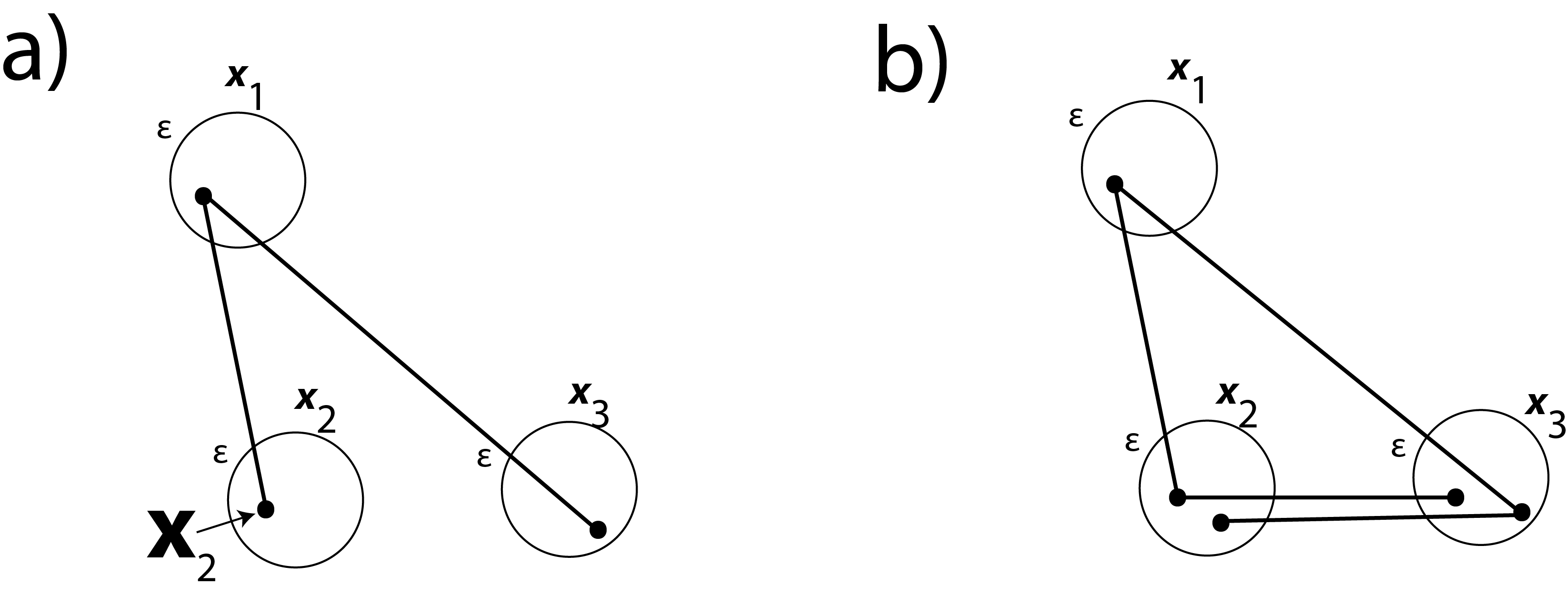
In order that a putative hidden-variable theory satisfies (17), it is necessary that, in addition to the real-world run where the particles were measured with nominal settings , the same particles (same ) could have been measured with nominal settings and with definite outcomes . We will consider these hypothetical worlds in turn.
For the first, keeping fixed, Alice continues to choose the nominal setting , whilst Bob hypothetically chooses the nominal setting . Since , then keeping and fixed, is fixed. By contrast, keeping fixed but transforming to implies a hypothetical change in Bob’s exact setting from to some (unknown) . This transformation is consistent with RaQM as long as the rationality conditions (13) and (14) hold. It is therefore necessary that and that where denotes the angle between the great circles and at the point of intersection. There are plenty of exact settings in the neighbourhood for for which these rationality constraints are satisfied.
But now, c.f. the third term in (17), we consider the hypothetical world where, keeping fixed, Alice chooses the nominal direction and Bob . With , is fixed by its value for the first hypothetical world. We now invoke the key property of the singlet state: if the measurement outcome was (say) when Bob’s exact setting was , then the measurement outcome will be in a hypothetical world where Alice’s exact setting was . Hence, considering the exact settings corresponding to the third term in (17), and must both be held fixed at their previously determined values. However, appealing to the Impossible Triangle Corollary, if and are rational and if is rational and not precisely a multiple of (gravitational waves from Andromeda will help ensure that), then cannot be rational. See Fig 1.
In essence, for each run in a Bell experiment, one of the two counterfactual runs is inconsistent with the rationality constraints of the hidden variable model and therefore must be assigned a probability . Put another way
| (18) |
where, to emphasise, all orientations in (18) are nominal. If one configuration occurs in reality (so that its probability is not identically zero) then (18) implies that (1) is violated.
5.2 The CHSH Inequality
This is a straightforward extension of the argument above though we no longer use the singlet property that, with the same exact settings, Alice and Bob must have opposite measurement outputs. Here , , and (with , as before) denote four disks (i.e. nominal settings) on the 2-sphere of orientations. In a given run where Alice chooses and Bob , we write the corresponding exact settings as , where
| (19) |
In order that a putative hidden-variable theory satisfies (2), it is necessary that, in addition to the real-world run, the same particles (with the same ) could have been measured with nominal settings , and , with definite outcomes .
As before, with , , , , we seek two exact settings , such that:
| (20) |
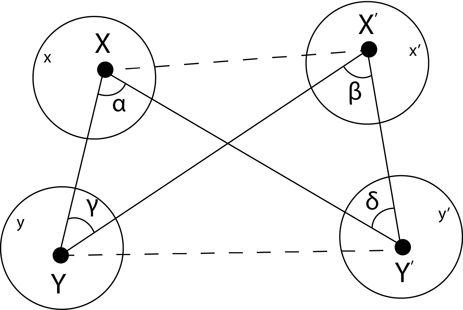
and, see Fig 2,
| (21) |
By repeated application of the Impossible Triangle Corollary, we now show it is impossible to satisfy (20) and (21).
We do this again by contradiction. Suppose that (20) and (21) are satisfied and consider the two triangles and . By the cosine rule for spherical triangles for each of the two triangles
| (22) |
Subtracting these equations then
| (23) |
must be rational. Writing , , then we can write
| (24) |
where are rational. However, by Niven’s Theorem, providing and are not precise multiples of , and must be irrational, hence and must be irrational. Moreover they must be independently irrational since and can be varied independently of one another. Hence generically must be irrational which is the contradiction we are looking for.
This in turn leads to the following general conclusion. In the situation where Alice chose and Bob , then, keeping the particles’ hidden variables fixed, at least one of the three counterfactual choices must violate the rationality conditions: 1) Alice and Bob chose and , Alice and Bob chose and , or Alice and Bob chose and . Similar to (18)
| (25) |
If , i.e. one configuration occurs in reality then (25) implies that (1) is violated. As with Bell’s 1964 inequality, the Impossible Triangle Corollary implies that (1) is violated without conspiracy.
It can be noted that since RaQM is based on an arbitrarily fine discretisation of complex Hilbert Space, by letting be sufficiently large, RaQM must violate Bell’s inequality as closely we like to the quantum mechanical violation of Bell’s inequality.
5.3 Local Causality
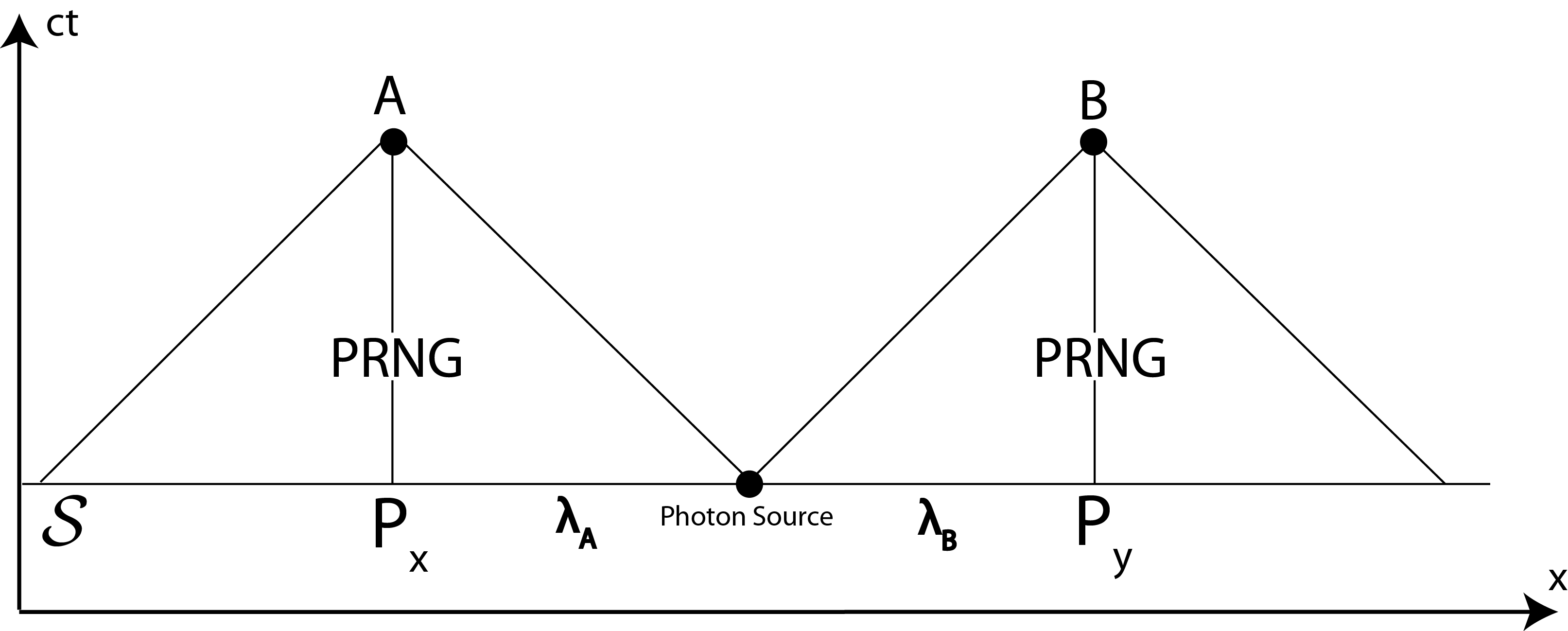
Fig 3 illustrates a space-time diagram where a photonic source emits two entangled photons. is a spacelike hypersurface through the event where the particles were emitted by the source. The photons are measured by Alice and Bob’s detectors with nominal settings and and exact settings and . The nominal settings are determined by two PRNGs shown in the figure. By the discussion above, the particle’s hidden variables , together with the parities and , determine these exact settings. We suppose that, consistent with the counterfactual violation of (19) and (20), but and
We divide into two components, corresponding to information in the past light cone of Alice’s measurement event, and corresponding to information in the past light cone of Bob’s measurement event. We write Alice and Bob’s measurement outcomes () in the form:
| (26) |
Whatever the values of and in (26), it is never the case that
| (27) |
where , describe perturbed data on (see Fig 3). That is to say, a hypothetical intervention in space-time which alters either Bob’s PRNG input or the hidden variable in the past light cone of Bob’s measurement event, keeping and fixed, and changes Alice’s measurement outcome, violates the rationality conditions (19) and (20). In simple words this implies that Alice’s measurement outcome does not depend on Bob’s measurement settings - the essence of locality. The space-time events at are irrelevant for determining the event because any intervention which changes keeping the data on fixed is inconsistent with the putative model and hence does not define a putative event in space time. But this is precisely Bell’s characterisation of local causality in La Nouvelle Cuisine - see Fig 4 in [6]. Put another way, the event is entirely determined by data on , the subset of contained on and in the past lightcone of - the essence of relativistic causality.
6 Objections to Superdeterminism
Below we address some of the objections that have been raised against superdeterminism with the RaQM/invariant set model in mind.
6.1 The Drug Trial
Each human in a drug trial is unique; having unique DNA for example. However, the characteristics used to allocate people randomly to the active drug or placebo groups are based on coarse-grain attributes. Are they young or old? Are they male or female? Are they black or white? We typically assume the two groups contain equal numbers of such coarse-grain attributes. In a conspiratorial drug trial, the selection process is manipulated so that the two groups do not contain equal numbers of coarse-grain attributes.
Although RaQM violates (1), it does not violate any version of (1) where coarse-grained hidden variables are used in place of hidden variables. For large enough , it is always possible to find counterfactual worlds which satisfy the rationality constraints in a coarse-grained volume of state space, no matter how small is . That is to say, in any sufficiently-large ensemble of individual runs,
| (28) |
where denotes a coarse-grained value of and denotes a frequency of occurrence. In this sense, (28) does not imply (1) and the drug trial conspiracy is an irrelevance to RaQM.
6.2 Fine Tuning
The fine-tuned objection (e.g. [4]) rests on the notion that superdeterminism appears to require some special, atypical, initial conditions. Perhaps one might view an initial state lying on a fractal attractor as special and atypical - after all a seemingly tiny perturbation (changing keeping fixed) can take the state of the universe off its invariant set . Although the Euclidean metric accurately describes distances in space-time, the -adic metric is more natural in describing distances in state space when the inherent geometry of state space is fractal [25]. From the perspective of the -adic metric, a fractal invariant set is not fine-tuned: a perturbation which takes a point off is a large perturbation (of magnitude at least ), even though it may appear very small from a Euclidean perspective. Conversely, perturbations which map points of to points of can be considered small amplitude perturbations.
Similarly, we must ask with respect to what measure are states on deemed atypical. Although states on are atypical with respect to a uniform measure on the Euclidean space in which is embedded, they are manifestly typical with respect to the invariant measure of [20].
In claiming that a theory is fine tuned, one should first ask with respect to which metric/measure is the tuning deemed fine - and then ask whether this the natural metric/measure to assess fineness.
6.3 Singular Limits and Aaronson’s Challenge
Aaronson’s challenge (see the Introduction) raises a more general question: what is the relationship between a successor theory of physics and its predecessor theory? There is a subtle but important relationship brought out explicitly by Michael Berry [9] that is of relevance here.
Typically an old theory is a singular limit of a new theory, and not a smooth limit, as a parameter of the new theory is set equal to infinity or zero. A singular limit is one where some characteristic of the theory changes discontinuously at the limit, and not continuously as the limit is approached. Berry cites as examples the old theory of ray optics is explained from Maxwell theory, or the old theory of thermodynamics is explained from statistical mechanics. His claim is that old theories of physics are typically singular limits of new theories.
If quantum theory is a forerunner of some successor superdeterministic theory, and Berry’s observation is correct, quantum mechanics is likely to be a singular limit of that superdeterministic theory. Here the state space of quantum theory arises at the limit of RaQM, but not before. For any finite , no matter how big, the incompleteness property that led to the violation of (1) holds. However, it does not hold at . From this point of view, quantum mechanics is indeed a singular limit of RaQM’s discrete Hilbert space, at . It is interesting to note that pure mathematicians often append the real numbers to sets (‘adeles’) of -adic numbers, at . However, the properties of -adic numbers are quite different to those of the reals for any finite no matter how big. Here the real-number continuum is the singular limit of the -adics at . The relationship between QM and RaQM is very similar.
In physics, it is commonplace to solve differential equations numerically, i.e. to treat discretisations as approximations of some continuum exact equations, such that when the discretisation is fine enough, the numerical results are as close as we require to the exact continuum solution. This is not a good analogy here. A better analogy is analytic number theory, considered as an approximation to say the exact theory of prime numbers. If one is interested in properties of primes for large primes, treating as if it were a continuum variable can provide excellent results. However, here the continuum limit is the approximation and not the exact theory.
Contrary to Aaronson’s statements, the singular relationship between a superdeterministic theory and quantum mechanics is exactly as one would expect from the history of science.
6.4 Free Will
Superdeterminism is often criticised as denying experimenter free will. Nobel Laureate Anton Zeilinger put it like this [51]:
We always implicitly assume the freedom of the experimentalist… This fundamental assumption is essential to doing science. If this were not true, then, I suggest, it would make no sense at all to ask nature questions in an experiment, since then nature could determine what our questions are, and that could guide our questions such that we arrive at a false picture of nature.
A clear problem here is that the notion of free will is poorly understood [24] and therefore hard to define rigorously. It was for this reason that Bell introduced his PRNG gedanken experiment - to show that it was possible to discuss (1) and its potential violation without invoking free will.
Nevertheless, to avoid the charge of conspiracy, an experimenter must be able to choose in a way which is indistinguishable from a random choice. For the present purposes we can think of this as being consistent with free will. For this reason, experimenters have found increasingly whimsical ways of choosing measurement settings - such as bits from a movie, or the wavelength of light from a distant quasar - in an attempt to mimic randomness.
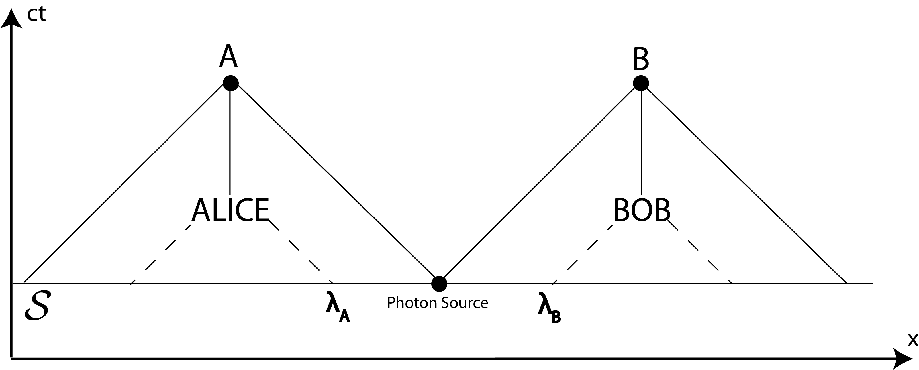
In Fig 4 we replace the two PRNGs in Fig 3 by Alice and Bob’s brains. It is well known that brains are low-power noisy systems [43] [36] where neurons can be stochastically triggered. In practice, the source of such stochasticity is thermal noise. However, such noise - arising from the collision of molecules - will have an irreducible component due to the Andromedan butterfly effect. In such circumstances, as discussed in Section 3, this can render the action of the brain non-computational. In particular, if we were to construct a model of Alice and Bob’s brains which are driven by the subset of data on (or indeed any subset), this model will not provide reliable predictions of their brains’ decisions. This surely provides evidence of our ability to choose in ways which are for all practical purposes random.
However, the Invariant Set Postulate provides insights which may help shed new light on the age-old dilemma of free will. Consider two possible invariant sets and . Here, for given , we suppose permits the settings and in a Bell experiment, whilst, keeping fixed, permits the settings and . These invariant sets differ (very slightly) in terms of their geometries, i.e. in terms of the (underlying deterministic) laws of physics.
If Alice and Bob are free to choose their measurement settings, then, prior to their choosing, all observations of the universe must be consistent with the universe belonging to either of the and . However, once Alice and Bob have chosen, not only is one of and consistent with available observations, the other becomes inconsistent with the supposed deterministic laws of physics.
Suppose Alice and Bob chose and let denote a state of the universe prior to Alice and Bob choosing. The question then arises: was it always the case - even before Alice and Bob chose - that and not ? Or did the very act of Alice and Bob choosing result in rather than ? In thinking about these questions, it is important to distinguish determinism from pre-destination. In a conventional deterministic initial-value problem, initial conditions are specified independently from evolutionary laws and the evolved state is predestined from the initial state. By contrast, if one thinks of the geometry of the invariant set as primitive, then the choices Alice and Bob make are no more ‘predestined’ from than is predestined from their choices. Instead, all one can say is that, because of determinism, the earlier and later states must be dynamically consistent. Importantly, as a global state space geometry, is consistent with what Adlam calls an ‘all at once’ constraint [2]. One could say that the geometric specification of , and hence whether , depends as much on states on to the future of as on states to the past of . This future/past duality exists because neither the proposition , nor Alice and Bob’s choice given , is computational (in our finite system it is computationally irreducible).
Hence, is it both true that (rather than ) before Alice and Bob chose, and also true that the act of choosing required rather than . Importantly, as there is no notion of temporal causality in state space, it would be wrong to call this latter fact retrocausality. Simply, it is a consequence of being an all-at-once constraint. This type of analysis helps explain the so-called delayed choice paradoxes in quantum physics.
It is possible to conclude not only that experimenter choices are indeed freely made (Nobel Laureates can be assured that their brains are not being subverted), but that these choices can determine which states of the universe are consistent with the laws of physics and which not (surely a fitting role for Nobel Laureates). This has some significant implications for the role of intelligent life in the universe more generally, which the author will discuss elsewhere.
7 Experimental Tests
A key result from this paper is that we will not be able to detect non-conspiratorial superdeterministic violations of (1) by studying frequencies of measurement outcomes in a Bell experiment. We must look for other ways of testing such theories.
Of course, QM is exceptionally well tested and if a superdeterministic theory is to replace QM, it must clearly be consistent with results from all the experiments which support QM. Here RaQM has a free parameter , which, if large enough, can replicate all existing experiments. This is because with large enough , discretised Hilbert space is fine enough that it replicates to experimental accurace the probabilistic predictions of a theory based on continuum Hilbert space (and Born’s Rule to interpret the squared modulus of a state as a probability - something automatically satisfied in RaQM). Conversely, however, if is some finite albeit large number, then in principle an experiment with free parameter can study situations where where there might be some departure between reality and QM [21].
One conceivable test of RaQM vs QM probes the finite amount of information that can be contained in the quantum state vector (in RaQM qubits are represented by bit strings of length ). In RaQM, the finite information encoded in the quantum state vector will limit the power of a general purpose quantum computer, in the sense that RaQM predicts the exponential increase in quantum compute speed with qubit number for a range of quantum algorithms may generally max out at a finite number of qubits.
The key question concerns the value of . Could it be related to the number of collisions in the Andromeda butterfly effect? We will return to this elsewhere.
8 Conclusions
Attempts to develop models which violate (1) do not justify the derision from a number of researchers in the quantum foundations community over the years. Not least, Bell himself did not treat the possible violation of (1) with derision and accepted that seemingly reasonable ideas about the properties of physical randomisers might be wrong - for the purposes at hand. .
A superdeterministic (and hence deterministic) model has been proposed which is not conspiratorial, is locally causal, does not deny experimenter free choice and is not fine tuned with respect to natural metrics and measures. The model, based on a discretisation of Hilbert space, is not a classical hidden-variable model, i.e. it derives its properties from post-quantum-theory mathematical science (particularly that of non-computability and computational irreducibility). By considering the continuum of complex Hilbert Space as a singular limit of a superdeterministic discretisation of complex Hilbert Space, Aaronson’s challenge to superdeterminists, to show how a superdeterministic model might gloriously explain quantum mechanics, can be met.
One of the most important conclusions of this paper is that we need to be extremely cautious when invoking the notion of an ‘intervention’ in space time, at least in the context of fundamental physics. Such interventions form the bedrock of Pearl’s causal inference modelling [38], and causal inference has been used widely in the quantum foundations community to try to analyse the causal structure of quantum physics e.g. [52] [40]. Here we distinguish between two types of intervention: one that is consistent with the laws of physics and one that is not. The effect of the former type of intervention, if it is initially contained within a localised region of space-time, must propagate causally in space-time, constrained by the Lorentzian metric of space time. By contrast, the latter type of intervention simply perturbs a state of the universe from a part of state space where the laws of physics hold, to a part of state space where the laws of physics do not hold. If this superdeterministic model is correct, theories of quantum physics based on causal inference models which adopt an uncritical acceptance of interventions will give misleading results.
The results of this paper suggest that the way gravity interacts with matter may be central to understanding the reasons why the universe can be considered a holistic dynamical system evolving on an invariant set, and hence why Hilbert space should be discretised. This suggests that instead of looking for a quantum theory of gravity, we should instead be looking for a gravitational theory of the quantum [34] [39]. However, importantly, the results here suggest such a theory will not be found by probing smaller and smaller regions of space-time, ultimately the Planck scale. It will instead be found by incorporating into the fundamental laws of physics, the state-space geometry of the universe at its very largest scales [36]. Planck-scale discontinuities in space-time may instead be an emergent property of such (top-down) geometric laws of physics.
In this regard, a recent proposal [31] for synthesising quantum and gravitational physics describes gravity as a classical stochastic field. The latter is consistent with our discussion of the Andromedan butterfly effect. However, it is not consistent with our discussion of Bell’s inequality. On the other hand, if one simply acknowledges that a stochastic gravitational field is a ‘for all practical purposes’ representation of a chaotic system evolving on a fractal invariant set, then Oppenheim’s model may become consistent with both the proposed superdeterministic violation of Bell’s inequality and with realism and the relativistic notion of local causality.
In the author’s opinion, this is the real message - not non-locality, indeterminism or unreality - behind the violation of Bell’s inequality.
Acknowledgements
My thanks to Emily Adlam, Jean Bricmont, Harvey Brown, Michael Hall, Jonte Hance, Inge Svein Helland, Sabine Hossenfelder, Tim Maudlin and Chris Timpson for helpful discussions and/or useful comments on an early draft of this paper. The author gratefully acknowledges the support of a Royal Society Research Professorship.
References
- [1] S. Aaronson. On tardigrades, superdeterminism and the struggle for sanity. https://scottaaronson.blog/?p=6215, 2022.
- [2] E. Adlam. Two roads to retrocausality. Sythese, 200, 2022.
- [3] M. Araujo. Superdeterminism is unscientific. https://mateusaraujo.info/2019/12/17/superdeterminism-is-unscientific/, 2019.
- [4] A. Baas and B. LeBihan. What does the world look like according to superdeterminism? British Journal for the Philosophy of Science, 73.4:555–572, 2023.
- [5] J.S. Bell. On the Einstein-Podolsky-Rosen paradox. Physics, 1:195–200, 1964.
- [6] J.S. Bell. Speakable and unspeakable in quantum mechanics. Cambridge University Press, 2004.
- [7] J.S. Bell, A.Simony, M.A.Horne, and J.F.Clauser. An exchange on local beables. Dialectica, 39:85–110, 1985.
- [8] M. Berry. Regular and irregular motion. American Institute of Physics Conference Proceedings Number 46, 1985.
- [9] M Berry. Singular limits. Physics Today, 55:10–11, 2002.
- [10] L. Blum, F.Cucker, M.Shub, and S.Smale. Complexity and Real Computation. Springer, 1997.
- [11] R. Buniy, S. Hsu, and A. Zee. Is Hilbert space discrete. Phys.Lett., B630:68–72, 2005.
- [12] R. Buniy, S. Hsu, and A. Zee. Discreteness and the origin of probability in quantum mechanics. arXiv:hep-th/0606062, 2006.
- [13] S. Carroll. Completely discretized, finite quantum mechanics. arXiv:2307.11927, 2023.
- [14] Eddy K. Chen. Bell’s theorem, quantum probabilities and superdeterminism. arXiv:2006.08609, 2020.
- [15] N.J. Cornish. Fractals and symbolic dynamics as invariant descriptors of chaos in general relativity. arXiv.org/gr-qc/9709036, 1997.
- [16] S. Dube. Undecidable problems in fractal geometry. Complex Systems, 7:423–444, 1993.
- [17] G.F.R. Ellis, K.A.Meissner, and H.Nicolai. The physics of infinity. Nature, 14:770–772, 2018.
- [18] S. Goldstein, T. Norsen, D.V.Tausk, and N.Zanghi. Bell’s theorem. http://dx.doi.org/10.4249/scholarpedia.8378, 2011.
- [19] M.J.W. Hall. Local deterministic model of singlet state correlations based on relaxing measurement independence. Phys. Rev. Lett., 105:250404, 2011.
- [20] Jonte R. Hance, Sabine Hossenfelder, and Tim N. Palmer. Supermeasured: Violating bell-statistical independence without violating physical statistical independence. Foundations of Physics, 52(4):81, Jul 2022.
- [21] J.R. Hance and S. Hossenfelder. What does it take to solve the measurement problem? arXiv:2206.10445, 2022.
- [22] Sabine Hossenfelder and Tim Palmer. Rethinking superdeterminism. Frontiers in Physics, 8:139, 2020.
- [23] J. Jahnel. When does the (co)-sine of a rational angle give a rational number? arXiv:1006.2938, 2010.
- [24] R. Kane. Free Will. Blackwell, 2002.
- [25] S. Katok. p-adic Analysis compared with Real. American Mathematical Society, 2007.
- [26] E.N. Lorenz. Deterministic nonperiodic flow. J.Atmos.Sci., 20:130–141, 1963.
- [27] E.N. Lorenz. The predictability of a flow which possesses many scales of motion. Tellus, 21:289–307, 1969.
- [28] T. Maudlin. Quantum non-locality and relativity. Wiley-Blackwell, 2011.
- [29] T. Maudlin. Tim maudlin and palmer: Fractal geometry, non-locality, bell. https://www.youtube.com/watch?v=883R3JlZHXE, 2023.
- [30] I. Niven. Irrational Numbers. The Mathematical Association of America, 1956.
- [31] Jonathan Oppenheim. A postquantum theory of classical gravity? Phys. Rev. X, 13:041040, Dec 2023.
- [32] T.N. Palmer. A local deterministic model of quantum spin measurement. Proc. Roy. Soc., A451:585–608, 1995.
- [33] T.N. Palmer. The invariant set postulate: a new geometric framework for the foundations of quantum theory and the role played by gravity. Proc. Roy. Soc., A465:3165–3185, 2009.
- [34] T.N. Palmer. Quantum theory and the symbolic dynamics of invariant sets: Towards a gravitational theory of the quantum. arXiv:1210.3940, 2012.
- [35] T.N. Palmer. Discretization of the Bloch sphere, fractal invariant sets and Bell’s theorem. Proc. Roy. Soc., https://doi.org/10.1098/rspa.2019.0350, arXiv:1804.01734, 2020.
- [36] T.N. Palmer. The Primacy of Doubt. Oxford University Press, 2022.
- [37] T.N. Palmer. Quantum physics from number theory. arXiv:2209.05549, 2022.
- [38] J. Pearl. Causal and counterfactual inference. The Handbook of Rationality. The MIT Press, pages 427–438, 2021.
- [39] R. Penrose. On the gravitization of quantum mechanics 1: Quantum state reduction. Foundations of Physics, 44:557–575, 2014.
- [40] H. Price and K. Wharton. Entanglement swapping and action at a distance. Foundations of Physics, 51:105, 2021.
- [41] R. Readhead. Incompleteness Nonlocality and Realism. Oxford University Press, 1992.
- [42] A. M. Robert. A Course in p-adic Analysis. Springer ISBN 0-387-98660-3, 2000.
- [43] E.T.. Rolls and G. Deco. The Noisy Brain. Oxford University Press, 2012.
- [44] S. Scanrani. Bell Nonlocality. Oxford Graduate Texts, 2019.
- [45] M. Schwartz. Statistical mechanics lecture 3. https://scholar.harvard.edu/files/schwartz/files, 2019.
- [46] L. Susskind. Fractal flows and time’s arrow. arXiv:1203.6440, 2012.
- [47] G. ’tHooft. The Cellular Automaton Interpretation of Quantum Mechanics. Springer, 2016.
- [48] J. A. Wheeler. Information, Physics, Quantum: The Search for Links. The Santa Fe Institute Press, 2023.
- [49] H.M. Wiseman and E.G.Cavalcanti. Causarum investigatio and the two Bell’s theorems of John Bell. arXiv:1503.06413, 2015.
- [50] S. Wolfram. A New Kind of Science. Wolfram Media, 2002.
- [51] A. Zeilinger. Zeilinger on superdeterminism. https://www.physicsforums.com/threads/zeilinger-on-superdeterminism.742415, 2014.
- [52] E. Wolfe Zjawin, B. and R.W. Spekkens. Restricted hidden cardinality constraints in causal models. arXiv:2109.05656, 2021.