A simplified spatial+ approach to mitigate spatial confounding in multivariate spatial areal models
Abstract
Spatial areal models encounter the well-known and challenging problem of spatial confounding. This issue makes it arduous to distinguish between the impacts of observed covariates and spatial random effects. Despite previous research and various proposed methods to tackle this problem, finding a definitive solution remains elusive. In this paper, we propose a simplified version of the spatial+ approach that involves dividing the covariate into two components. One component captures large-scale spatial dependence, while the other accounts for short-scale dependence. This approach eliminates the need to separately fit spatial models for the covariates. We apply this method to analyse two forms of crimes against women, namely rapes and dowry deaths, in Uttar Pradesh, India, exploring their relationship with socio-demographic covariates. To evaluate the performance of the new approach, we conduct extensive simulation studies under different spatial confounding scenarios. The results demonstrate that the proposed method provides reliable estimates of fixed effects and posterior correlations between different responses.
Keywords: Crimes against women; M-models; Spatial confounding; Spatial+.
1 Introduction
Univariate spatial models for areal count data have been a prevailing approach in smoothing standardized incidence or mortality ratios of chronic diseases. Though these techniques have been mainly applied to study incidence and mortality of different types of cancer, other applications exist. A very interesting one is the study of crimes against women in India (see Vicente et al., 2020a, ) where gender based violence is an issue. Univariate modelling is crucial for visualizing the spatial patterns of crimes against women. However, adopting a multivariate approach can enhance the accuracy of estimates and reveals latent correlations between the spatial patterns of crimes (Vicente et al., 2023b, ). This is essential for gaining a better understanding of this complex and multifaceted problem, and ultimately, for effective prevention.
Despite the substantial growth in research on multivariate spatial models for areal count data, their practical application is still limited due to the computational complexity involved in their implementation. While various approaches exist for constructing multivariate models for disease mapping (see for example MacNab,, 2018), this study follows the corregionalization framework (Jin et al.,, 2007). In particular, the research by Martinez-Beneito, (2013) presents a comprehensive corregionalization approach that encompasses most of the multivariate methodologies suggested in the existing literature. However, this approach can be computationally prohibitive and an alternative reformulation known as M-models (Botella-Rocamora et al.,, 2015) is considered.
Incorporating potential risk factors (covariates) into a multivariate spatial model is important to evaluate the potential relationship between the covariates and the individual responses. This can contribute to gain knowledge about crimes against women, a multifaceted problem affected by social, religious, or economic characteristics with intricate interactions difficult to disentangle. However, when both, the covariate and spatial random effects enter in the model, an important challenge appears. Namely, how to separate the fixed effects from the spatial random effects. This is known as “spatial confounding”. When spatial random effects enter in the model, a change in the fixed effect estimates is observed compared to a simple linear or generalized linear model (GLM) that does not consider spatial correlation. Although spatial confounding has usually been considered as a collinearity problem between fixed effects and spatial random effects (see for instance Reich et al.,, 2006; Hodges & Reich,, 2010; Hughes & Haran,, 2013; Hanks et al.,, 2015; Page et al.,, 2017; Adin et al.,, 2023), there is not a unique general definition neither a unique solution. In fact, Gilbert et al., (2022) identify four different but related phenomena commonly referred as spatial confounding. In what follows, we consider that the effect of the unobserved covariates is approximated by spatial random effects in the model (Congdon,, 2013; Marques et al.,, 2022), and we seek procedures that can simultaneously avoid bias in the estimates of the fixed effects, reduce their variance, and appropriately smooth the relative risks.
Various procedures have been proposed in the literature to address spatial confounding in the univariate framework, with restricted spatial regression (RSR) (Reich et al.,, 2006) being the most extended approach. RSR effectively deals with the collinearity between the covariate and spatial random effects by constraining the spatial random effects to lie in the orthogonal complement of the space spanned by the covariates. As a result, RSR provides fixed effects estimates that are equivalent to those obtained using a simple GLM. Additionally, the variance of the RSR fixed effects estimates falls somewhere between the variance obtained with the simple GLM and the variance obtained with the classical disease mapping spatial model (Reich et al.,, 2006; Hodges & Reich,, 2010). Consequently, RSR might help prevent variance inflation of the fixed effects estimates, a concern that is widely recognized in spatial modelling. However, recent evidence contradicts some prior beliefs about RSR. Khan & Calder, (2022) demonstrate that for normal responses, the variance of the fixed effects estimated with RSR is either equal to or lower than the variance obtained from the model without spatial random effects, leading to overly liberal inference. These authors also highlight potential issues of RSR for count data. Additionally, Gilbert et al., (2022) argue that RSR implicitly assumes the absence of unobserved covariates that overlap with the observed ones, as it forces the random effects to be orthogonal to the fixed effects. Furthermore, they support that the collinearity between the covariate and spatial random effects may not be a concern, but something expected if we assume the existence of unobserved covariates.
The spatial+ approach (Dupont et al.,, 2022) appears to be a promising method among the various alternatives for addressing spatial confounding. This is a two-step procedure that consists in removing spatial dependence from the covariate in a first step by fitting a spatial model to the covariate itself. Then, in the second step, a classical spatial regression model for the outcome is fitted replacing the covariate by the residuals obtained in the first step. In the univariate case, Urdangarin et al., (2023) conducted simulations to compare the fixed effects estimates of various approaches, including a simple GLM, the classical spatial model, the spatial+ approach, as well as other proposals such as RSR and transformed Gaussian Markov random fields (TGMRF) (Prates et al.,, 2015). Overall, the spatial+ method demonstrated superior performance in terms of fixed effect estimates. Recent procedures to deal with spatial confounding include spectral methods (Guan et al.,, 2022), and a joint Gaussian Markov random field model for the covariate and the response (see Marques et al.,, 2022).
This work has two main objectives: firstly, we aim to propose a modified spatial+ approach that alleviates spatial confounding eliminating the need for separately fitting spatial models for the covariates. Secondly, we seek to estimate the latent correlations between several responses. To deal with these two goals we use M-models incorporating the modified spatial+ method that offer a tailored approach by accommodating the inclusion of distinct covariates for each individual response. Moreover, these models provide the necessary flexibility to effectively address spatial confounding for each response. To illustrate the procedure, we analyse crimes against women, rapes and dowry deaths, in the districts of Uttar Pradesh in 2011 and we assess their relationship with some sociodemographic covariates. To examine how well our proposal recovers the fixed effects and the correlations between crimes, we have simulated several scenarios under spatial confounding. The data generating model includes one observed covariate that has a distinct regression coefficient for each individual response and additional variability. Model fitting and inference is carried out from a full Bayes approach, using integrated nested Laplace approximations (Rue et al.,, 2009).
The rest of the article is organized as follows. In Section 2, we introduce a simplified spatial+ approach for fitting spatial models (univariate or multivariate) without the need to fit a separate spatial model to the covariate. Section 3 reviews the multivariate spatial models making emphasis on the M-models. Section 4 discusses some model implementation details and identifiability constraints. In Section 5 we use the procedures to analyse two crimes against women, rape and dowry death, in Uttar Pradesh, India, in the year 2011. Section 6 presents an exhaustive simulation study. Finally, the paper ends with a discussion.
2 Simplified spatial+ approach
The spatial+ method (Dupont et al.,, 2022) is a two-step procedure designed to reduce bias in the fixed effect estimates of univariate spatial models by eliminating the spatial dependence of the covariates. The first step consists in fitting a spatial model to the covariate to remove the spatial dependence. Then, in the second step, the spatial model is fitted replacing the covariate by the residuals obtained in the first step. Here, we modify the spatial+ procedure to remove the spatial dependence of the covariate in a simpler way, avoiding fitting a spatial model to the covariate. We also extend the spatial+ approach to the multivariate framework.
Let us consider the following univariate spatial disease mapping model where, conditional on the relative risk , the number of counts in a given area , is assumed to follow a Poisson distribution
Here, is the number of expected counts and the log risk is modelled as
where is value of the covariate in the th area. In matrix form
| (1) |
where , is a column vector of ones of length , , and is the vector of spatial random effects with precision matrix , which may be different depending on the spatial prior used for . In this paper we consider one of the following priors: intrinsic conditional autoregressive (ICAR) prior (Besag,, 1974), proper conditional autorregresive (PCAR) prior (see for example Banerjee et al.,, 2015, chapter 4) or BYM2 prior (Riebler et al.,, 2016). In more detail, , where the precision matrix depends on the spatial prior chosen:
-
•
ICAR: where is the precision parameter, is a diagonal matrix with the number of neighbours of each area in the main diagonal, and is a binary adjacency matrix where each entry takes value if areas and are neighbours and 0 otherwise, and . Note that is the usual neighbourhood matrix where the th diagonal element is equal to the number of neighbours of the area , and the off diagonal elements if the areas and share a common border and 0 otherwise.
-
•
PCAR: , which provides a valid distribution if and only if being and the minimum and maximum eigenvalues of (Jin et al.,, 2007). When , the PCAR becomes the ICAR prior.
-
•
BYM2: where is an identity matrix and is the Moore–Penrose generalized inverse of the scale-transformed precision matrix (for more details about this scale transformation see Riebler et al.,, 2016). In this prior, represents the proportion of the marginal variance explained by the structured effect.
The spatial+ approach assumes that the covariate is modelled as
| (2) |
where are the coordinates (longitude and latitude) of the centroid of the small areas, is a smooth function to be estimated using thin plate splines, and , where is the standard deviation of the independent and identically distributed errors. The residuals of this model are defined as and the spatial model (1) is fitted replacing the covariate of interest by the residuals .
Urdangarin et al., (2023) suggest an alternative to model (2) to remove the spatial dependence in the covariate. It consists in fitting a linear model where the response is now the covariate , and some of the eigenvectors of the spatial precision matrix act as regressors. Each eigenvector captures spatial dependence at different scales, the eigenvectors corresponding to the lowest non-null eigenvalues being the smoothest ones. Thus, the number of eigenvectors included as covariates in the model defines the quantity of spatial dependence removed from . The simulation study performed by these authors indicates that with the new approach the fixed effects are recovered better than using thin plate splines. However this approach also requires fitting a linear model to the covariate.
In this paper, we introduce a simplified spatial+ approach without the need of fitting a spatial model to the covariate. This simplified spatial+ approach is a simpler and more straightforward procedure. Consider the spectral decomposition of the spatial precision matrix, , where is an orthogonal matrix whose columns are the eigenvectors of and is a diagonal matrix with the eigenvalues of in the main diagonal. Note that for connected graphs up to a normalizing constant and . Since the eigenvectors of form a basis of and contain spatial information at different scales, we now express the covariate as a linear combination of the eigenvectors , , that is,
Assuming that the collinearity between the fixed and random effects primarily arises from the eigenvectors associated with the lowest non-null eigenvalues, that is, presuming that the eigenvectors linked to the high eigenvalues remain unconfounded with the covariate (equivalent to the unconfoundedness at high frequencies assumption for identifiability in the work by Guan et al.,, 2022), we split the covariate into two parts
| (3) |
where comprises large-scale eigenvectors associated with the lowest eigenvalues, contains the rest of eigenvectors, and is the number of large-scale eigenvectors assigned to . Finally, the spatial model (1) is fitted replacing the covariate by its spatially decorrelated part as
| (4) |
We have verified that the spatial+ proposed in Urdangarin et al., (2023) and the simplified spatial+ proposed here yield to almost identical results in univariate models.
In the next section, we introduce multivariate disease mapping models and extend the modified spatial+ approach to this framework.
3 Multivariate ecological spatial areal models
Multivariate spatial areal models handle two types of dependencies: within-response dependence, often characterized by spatial dependence, and between-response correlations, which typically lack of a specific structure and pose a challenge. Multivariate models, in general, have the potential to provide more reliable risk estimates compared to traditional univariate models. In this paper, we employ multivariate ecological regression models to examine potential linear associations between the responses and a covariate of interest.
Let now and denote, respectively, the number of observed and expected cases in the th small area and th crime , and assume that follows a Poisson distribution conditioned on the relative risk , that is
The log-risk is modelled as
| (5) |
where is the intercept of th crime, is a crime-specific regression coefficient related to the covariate and is the spatial effect of area and crime . Model (5) can be expressed in matrix form as
| (6) |
where is the vector of relative risks with for , is a identity matrix, is a vector of ones of length and refers to the Kronecker product of two matrices. The vectors of crime-specific intercepts and regression coefficients are denoted by and respectively. Finally, where is the vector of spatial random effects of the th crime. The within and between-crime dependence is introduced through the precision/covariance matrix of the spatial random effect. In particular the following prior distribution with Gaussian kernel is assumed for with precision matrix
| (7) |
where is any square root of the symmetric and positive definite between-crime covariance matrix , that is , and is the spatial precision matrix for the crime. The elements of the between-crime covariance matrix are all unknown and have to be estimated. Details about how the between-crime dependence is introduced in Model (6) through the matrix are provided below. Here can be the precision matrix of the ICAR, PCAR or BYM2 priors. For the ICAR prior, the precision matrix is the same for all crimes and has a separable structure, . Likewise, for the PCAR and BYM2 priors, if and for , we have the separable precision matrices and , respectively.
In the following, we review how to introduce spatial dependencies within crimes as well as the correlation between spatial patterns of different crimes through the M-models (Botella-Rocamora et al.,, 2015). In this paper, the multivariate models include a single covariate, but the proposed methodology can be extended to the case of multiple covariates.
To better understand how the M-models deal with the within and between-crime dependence, we rearrange the spatial effects into the matrix . Following Botella-Rocamora et al., (2015), can be expressed as
| (8) |
where the columns of the matrix are independent and follow a spatially correlated distribution to deal with spatial dependence within crimes, namely for each column . Then, the spatial covariance matrix of column is and it is usually known as the within th crime covariance matrix. The matrix induces dependence between the columns of , that is, it induces correlation between the spatial patterns of different crimes. A typical election for is to consider the lower triangular matrix of the Cholesky decomposition of the between-crime covariance matrix , however the effects of this election depend on the ordering of the crimes in the vector as pointed out by Martinez-Beneito, (2013) (see Appendix A.1 for details). To avoid this undesired situation, is any nonsingular matrix without any other restriction that satisfies the condition (Botella-Rocamora et al.,, 2015). Using that
(see for example Harville,, 2008, p. 345) where the vec operator stacks the columns of a matrix one under the other and , , and are conformable matrices for multiplication, it is obtained that
Then, the covariance matrix of is
| (9) | |||||
Clearly, the inverse of this matrix is the precision matrix in Equation (7).
To make the spatial random effects identifiable, appropriate sum-to-zero constraints must be contemplated. Here, we will consider the constraints proposed by Goicoa et al., (2018) for each crime. In addition, we fix the precision parameters of the spatial precision matrices at 1 to make the between-crime covariance matrix identifiable (Martinez-Beneito,, 2013). Note that in the case of separable covariance structures, we set the parameter as any change in scale in the within-crime covariance matrix can be compensated for by an appropriate change in the scale of the between-crime covariance matrix . Regarding non separable covariance structures, the between-crime covariance matrix will be identifiable if the precision parameters are fixed at 1. More precisely, setting (not necessarily equal to 1) only identifies up to scaling. In any case, fixing the precision parameters at 1 is not restrictive as the elements of the matrix control the degree of smoothing within each crime (see Appendix A.2 for details).
By estimating the entries of the matrix , the covariance structure between the spatial patterns of different crimes can be estimated as . Note that the entries of can be interpreted as coefficients in the regression of the log-relative risks on the columns of . Hence, they can be treated as fixed effects and assigning a zero-centred normal prior with large fixed variance is a reasonable choice. This is equivalent to assume a Wishart prior to , i.e. (see Botella-Rocamora et al.,, 2015, for more details ).
Finally, to deal with spatial confounding, the multivariate M-model (6) is fitted replacing the covariate by its spatially decorrelated part as
| (10) |
It is worth mentioning that Model (10) allows removing a different number of eigenvectors for each crime. That is
where is the part of the covariate that we retain for crime .
4 Model implementation
In this paper, models are fitted using the Integrated nested Laplace approximation (INLA) approach (Rue et al.,, 2009). INLA is designed for approximate Bayesian inference avoiding the convergence issues of MCMC techniques and saving computing time. Hence it has become very popular for performing Bayesian inference with a wide range of hierarchical models. The R package R-INLA (Lindgren & Rue,, 2015) has many models directly available and allows to implement other models using rgeneric or cgeneric constructions. The M-models are not directly available in R-INLA, so here we will use the rgeneric construction as in Vicente et al., 2020b .
The matrix involves parameters when only parameters are needed to determine the convariance matrix . Thus, to avoid overparameterization, when we consider the Wishart prior on the covariance matrix, , we use the Bartlett decomposition of Wishart-distributed matrices (see for example Peña & Irie,, 2022). More precisely, if , the Bartlett decomposition of is . Here is the Cholesky factor of and
| (12) |
where the diagonal and non-diagonal elements are independently distributed as and for with . Using the Bartlett decomposition we only use parameters instead of parameters. In our case, and then . Finally, to avoid dependence on the ordering of the crimes of , instead of estimating (which is upper triangular), we first compute and then we estimate , where are the eigenvalues of the between-crime covariance matrix and the columns of are the corresponding eigenvectors. Using this instead of the Cholesky square root in the global covariance matrix (9), we avoid dependence on the ordering of the crimes in . Details about the implementation of the Bartlett decomposition can be found in Vicente et al., 2023a . Finally, we note that the parameter can be absorbed by the elements of and we fix it at 1 for identifiability issues. We run the analysis with different values of and the results did not change.
Finally, we have considered a uniform distribution Unif(0,1) for the hyperparameters and of the PCAR and BYM2 spatial priors. Note that the Unif(0,1) prior on the parameters is used to consider only positive spatial correlations (see for example Martinez-Beneito & Botella-Rocamora,, 2019, Chap. 4, p.147). A normal distribution with mean 0 and precision 0.001 are given to crime-specific intercepts and regression coefficients . All the models are fitted using R version 4.2.3 and R-INLA package version 22.12.16 (dated 2022-12-23) with the simplified Laplace strategy. The full code and data to reproduce results are available at https://github.com/spatialstatisticsupna/Multivariate_confounding.
5 Illustration: joint analysis of rapes and dowry deaths in Uttar Pradesh in 2011
In this section we analyse jointly rapes and dowry deaths, two forms of crimes against women in the 70 districts of Uttar Pradesh in 2011. The main objective is to assess whether there is linear association between a covariate of interest and the relative risks of each crime using the multivariate models with the spatial+ approach defined in the previous sections.
Uttar Pradesh is the most populated state of India and it is located in the north of the country. Despite underreporting, the elevated number of rapes in India is a matter of concern (see Vicente et al.,, 2018, for the temporal evolution of rapes in Uttar Pradesh). Dowry death is deeply-rooted in the marriage system in India and it is related to the dowry. The dowry represents the goods that the bride’s family offers to the groom’s family before the marriage. Disputes related to the dowry are frequent and the use of violence against the bride to obtain a higher dowry is common. Sadly, this violence often ends in the dead of the woman. This is known as dowry death. Any death related to dowry, such as, murder or suicide of the woman within the first seven years of marriage is considered a dowry death (Vicente et al., 2020a, ). Although in 1961 the Dowry Prohibition Act was approved, the tradition of dowry is still widespread.
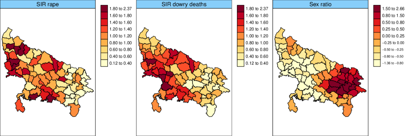
The minimum values for rapes and dowry deaths per district in 2011 are 2 and 6 respectively, whereas the maximum values are 89 and 95. So, the number of rapes and dowry deaths per district in 2011 is highly variable. Figure 1 displays the standardized incidence ratio (SIR) of rapes and dowry deaths in 2011. Some similarities between both spatial patterns can be observed with a Pearson correlation coefficient of 0.4471. Thus, it is sensible to analyse both crimes jointly. Figure 1 also shows the spatial pattern of the (standardized) covariate sex ratio defined as the number of females per 1000 males. Here, the goal is to assess the potential linear association between the sex ratio and the relative risks of rapes and dowry deaths. However, this task may not be straightforward due to the evident spatial pattern of the covariate sex ratio, and the addition of spatial random effects as a proxy of unobserved covariates can induce bias in the fixed effects estimates (spatial confounding).
Here we fit the M-models (6) and (10) introduced in Section 2. First, the covariate sex ratio is expressed as a linear combination of the eigenvectors of the precision matrix (see Equation (3)). Then we remove , the part of the linear combination containing the large scale eigenvectors associated with the lowest eigenvalues. The number of large-scale eigenvectors chosen depends on the dimensions of . Here, is between and , which represent 7% and 29% of all eigenvectors. Table 1 presents the notation of the M-models used. All the M-models are fitted considering ICAR, PCAR and BYM2 priors for the spatial random effects.
| Name | M-model | Covariate | ||
| M-Spatial | (6) | – | – | |
| M-SpatPlus64 | (10) | 5 | 64 | |
| M-SpatPlus59 | (10) | 10 | 59 | |
| M-SpatPlus54 | (10) | 15 | 54 | |
| M-SpatPlus49 | (10) | 20 | 49 |
Table 2 provides posterior means, posterior standard errors and 95% credible intervals of sex ratio for rapes () and dowry deaths () with different M-models. A negative linear association is observed between sex ratio and both crimes. For rapes, the 95% credible intervals always contain 0 irrespective of the models and the spatial prior, indicating a non-significant relationship between rapes and sex ratio. For dowry deaths, we observed a reduction of the posterior mean in the spatial+ models with respect to the spatial model. However, 95% credible intervals exclude with the M-Spatial, the M-SpatPlus64 and the M-SpatPlus59 models. In general, multivariate models with the spatial+ approach reduce the posterior standard deviations in comparison to the usual multivariate spatial model. Overall, the three spatial priors lead to similar fixed effects estimates, though some differences appears in the multivariate spatial models without the spatial+. The results are in line with previous literature as dowry death is the only crime against women that seems to be associated with sex ratio (see for example Mukherjee et al.,, 2001).
| Model | |||||||||
| Mean | SD | CI | Mean | SD | CI | ||||
| ICAR | M-Spatial | -0.1560 | 0.1050 | -0.3630 | 0.0500 | -0.1920 | 0.0600 | -0.3080 | -0.0720 |
| M-SpatPlus64 | -0.0750 | 0.0680 | -0.2090 | 0.0590 | -0.0940 | 0.0410 | -0.1730 | -0.0130 | |
| M-SpatPlus59 | -0.0750 | 0.0640 | -0.2010 | 0.0500 | -0.0810 | 0.0390 | -0.1580 | -0.0040 | |
| M-SpatPlus54 | -0.0720 | 0.0580 | -0.1860 | 0.0420 | -0.0430 | 0.0370 | -0.1150 | 0.0290 | |
| M-SpatPlus49 | -0.0870 | 0.0550 | -0.1960 | 0.0210 | -0.0460 | 0.0350 | -0.1150 | 0.0230 | |
| PCAR | M-Spatial | -0.2270 | 0.0950 | -0.4070 | -0.0330 | -0.2520 | 0.0570 | -0.3600 | -0.1350 |
| M-SpatPlus64 | -0.0750 | 0.0690 | -0.2100 | 0.0600 | -0.0970 | 0.0430 | -0.1830 | -0.0130 | |
| M-SpatPlus59 | -0.0770 | 0.0650 | -0.2060 | 0.0520 | -0.0840 | 0.0410 | -0.1640 | -0.0030 | |
| M-SpatPlus54 | -0.0720 | 0.0590 | -0.1890 | 0.0450 | -0.0440 | 0.0390 | -0.1200 | 0.0320 | |
| M-SpatPlus49 | -0.0870 | 0.0570 | -0.1990 | 0.0240 | -0.0460 | 0.0380 | -0.1200 | 0.0270 | |
| BYM2 | M-Spatial | -0.1800 | 0.0990 | -0.3720 | 0.0150 | -0.2500 | 0.0590 | -0.3620 | -0.1310 |
| M-SpatPlus64 | -0.0680 | 0.0670 | -0.2000 | 0.0650 | -0.1100 | 0.0430 | -0.1940 | -0.0260 | |
| M-SpatPlus59 | -0.0720 | 0.0640 | -0.1990 | 0.0550 | -0.0960 | 0.0410 | -0.1780 | -0.0150 | |
| M-SpatPlus54 | -0.0710 | 0.0610 | -0.1900 | 0.0480 | -0.0490 | 0.0390 | -0.1250 | 0.0270 | |
| M-SpatPlus49 | -0.0930 | 0.0590 | -0.2080 | 0.0220 | -0.0540 | 0.0380 | -0.1280 | 0.0200 | |
Table 3 presents the posterior median of the correlation between rapes and dowry deaths with their 95% credible intervals. The estimated correlations are about 0.3 but slight discrepancies are noted in the estimates depending on the model and the spatial prior. Multivariate spatial+ models with the PCAR prior point towards a significant correlation. However, the rest of models indicate that the correlation is not significant. Given that the lower bounds of the credible intervals are very close to zero, we might conclude that the correlation is on the verge of significance. Finally, to compare the models in terms of goodness of fit and complexity, we have computed the Deviance Information Criterion (DIC) and the Watanabe-Akaike Information Criterion (WAIC) (see Table 4). M-models with spatial+ improve slightly the fit compared to the M-Spatial model, but differences are negligible. This is expected as the spatial+ approach can be seen as a kind of reparameterization of the spatial model.
| Model | ICAR | PCAR | BYM2 | ||||||
| Median | CI | Median | CI | Median | CI | ||||
| M-Spatial | 0.3066 | -0.0677 | 0.6087 | 0.3127 | -0.0508 | 0.6177 | 0.2502 | -0.1483 | 0.5703 |
| M-SpatPlus64 | 0.3376 | -0.0090 | 0.6275 | 0.3698 | 0.0302 | 0.6503 | 0.3096 | -0.0722 | 0.6499 |
| M-SpatPlus59 | 0.3320 | -0.0151 | 0.6313 | 0.3601 | 0.0245 | 0.6361 | 0.3086 | -0.0021 | 0.6079 |
| M-SpatPlus54 | 0.3347 | -0.0056 | 0.6097 | 0.3713 | 0.0448 | 0.6304 | 0.2622 | -0.0688 | 0.5869 |
| M-SpatPlus49 | 0.3222 | -0.0185 | 0.6229 | 0.3657 | 0.0405 | 0.6245 | 0.2581 | -0.0368 | 0.5464 |
To summarize, different fixed effects are estimated for both crimes depending on the model fitted to the data. For rapes, the posterior mean of the sex ratio coefficient is negative but the 95% credible intervals do not point towards a significant negative association. For dowry deaths, the conclusions depend on the number of large-scale eigenvectors excluded in the M-models with spatial+. According to Urdangarin et al., (2023), in univariate spatial models with spatial+, removing 14% to 21% of eigenvectors could lead to unbiased fixed effect estimates. Here, M-SpatPlus59 and M-SpatPlus54 are the equivalent models to removing 14% and 21% of eigenvectors. The 95% credible interval of M-SpatPlus59 points towards a significant negative association between sex ratio and dowry deaths. Nevertheless, caution is recommended when reaching conclusions.
We have also run the models including other socioeconomic covariates. The results are omitted to save space. Among all the covariates analysed, only the covariate “number of burglaries” shows a significant positive linear association with rapes, but it does not show a significant association with dowry deaths. We have fitted all the previous M-models including both, sex ratio and burglaries as covariates but overall, the fixed effect estimates for each response do not change. The M-models proposed here allow removing different quantities of spatial dependence from each covariate, as well as the inclusion of specific covariates for a particular response. For example, the covariate burglary might be considered only for the analysis of rapes, while the sex ratio might be included only for dowry deaths.
| Model | ICAR | PCAR | BYM2 | |||
| DIC | WAIC | DIC | WAIC | DIC | WAIC | |
| M-Spatial | 959.1602 | 949.0371 | 961.2425 | 948.8055 | 959.7526 | 946.1454 |
| M-SpatPlus64 | 958.7318 | 945.9487 | 960.0558 | 944.6206 | 960.2536 | 943.0920 |
| M-SpatPlus59 | 958.8249 | 945.6563 | 960.0255 | 944.4730 | 960.3539 | 942.8094 |
| M-SpatPlus54 | 959.3916 | 945.3981 | 960.7766 | 944.4437 | 960.7177 | 943.4793 |
| M-SpatPlus49 | 959.3160 | 945.5091 | 960.9914 | 944.7533 | 960.3658 | 943.0917 |
6 Simulation study
In this section, we conduct two simulation studies, named Simulation study 1 and Simulation study 2, to evaluate the performance of the simplified spatial+ method in multivariate models in the presence of spatial confounding. For both simulation studies, we have employed the geographical configuration of Uttar Pradesh consisting of connected districts. Two related responses, denoted as crime 1 and crime 2 from now on, are generated. In Simulation study 1 we examine if the spatial+ method recovers the true fixed effects for each of the crimes when there is spatial confounding. Simulation Study 2 focuses on evaluating how well the multivariate models with the spatial+ technique simultaneously estimate the correlation between crimes and the fixed effects.
Simulation study 1: the data generating model includes the standardized covariate sex ratio of the real data analysis, denoted as , and two additional covariates, and . Both and play the role of unobserved covariates in the fitted model for crimes 1 and 2 respectively, and hence they can induce spatial confounding. The correlation between and , as well as the correlations between and and and are fixed. The fitted models do not include and . In more detail, the counts for crime 1 and crime 2 are simulated as follows,
| (15) | |||
| (16) |
where , , , , and is the vector of expected cases of the real case study. Two scenarios are simulated depending on the correlations between , and . Scenario 1 addresses moderate-high correlations between the covariates and Scenario 2 deals with moderate-low correlations.
-
•
Scenario 1: the correlations are , and . Here spatial confounding might be a major concern.
-
•
Scenario 2: the correlations are , and . In this case, spatial confounding might not be so severe.
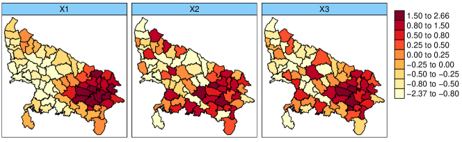
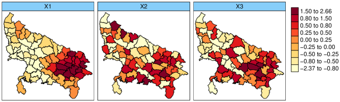
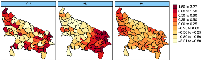
Figure 2 displays the standardized sex ratio covariate, along with the simulated covariates and . The first row illustrates the spatial patterns of these covariates for Scenario 1, while the second row presents the patterns for Scenario 2. For each of the scenarios a total of counts data sets are generated. To complete the simulation study, Supplementary material A presents the details about the data generating process of some additional scenarios, Scenarios 3, 4, 5 and 6, and their results. (Note that in Scenarios 5 and 6, and hence, confounding should not be an issue for crime 1.)
Simulation study 2: the aim of this simulation study is to see how well multivariate models with the spatial+ method estimate the fixed effects but also the correlation between crimes. The objective is to see whether the modified spatial+ method introduces some bias in the estimation of the between-crime correlations. Here, the data generating process is quite different to Simulation study 1. First, a vector of spatial effects, is generated as where the precision matrix follows the separable structure . The between-crime covariance matrix is conveniently expressed as
where , are the variances obtained with the M-Spatial model in the real data analysis and is the pre-defined linear correlation between crime 1 and crime 2. In a second step, a covariate is simulated such that its linear correlation with the spatial effects of crime 1, , and the spatial effects of crime 2, , is fixed. In more detail, data are generated as,
| (17) | |||
| (18) |
where , and is the vector of expected cases of the real case study. Now, and are considered. Two scenarios are simulated depending on the correlation between crimes, , and the correlations between the simulated and the spatial effects and . Scenario 1 addresses moderate-high correlations and Scenario 2 deals with low-moderate correlations.
-
•
Scenario 1: the correlations are , and . Here spatial confounding might be a major concern and the crimes are highly correlated.
-
•
Scenario 2: the correlations are , and . In this case, spatial confounding might not be so severe and the correlation between crimes is low.
Figure 3 shows the standardized simulated covariate and the spatial effects and for each of the crimes. The first row displays the spatial patterns for Scenario, 1 while the second row depicts those for Scenario 2. For each of the scenarios a total of counts data sets are generated. Supplementary material B presents the details about the data generating process of some additional scenarios, Scenarios 3, 4 and 5, and their results.
The simulated data are analysed using the same models as those employed in the real data analysis. All the models are fitted assigning ICAR, PCAR and BYM2 priors to the spatial random effects. The objective is to examine in more detail how the simplified spatial+ method recovers the true fixed effects in different scenarios and if the between-crime correlation estimates are affected by the method.
6.1 Simulation study 1: Results
The main goal of this simulation study is to evaluate the fixed effect estimates of the spatial+ method in multivariate models. Intuitively, the correlation between the unobserved covariates should be captured by the between-crime correlation matrix, so we will also look at those parameters.
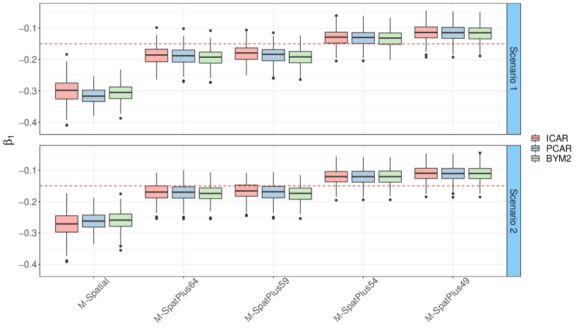
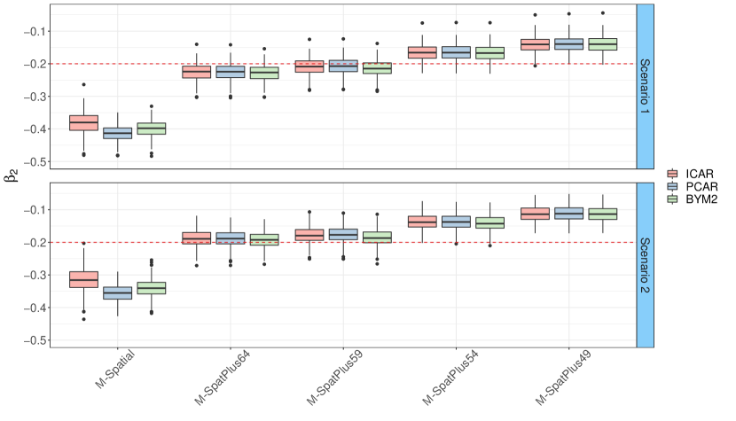
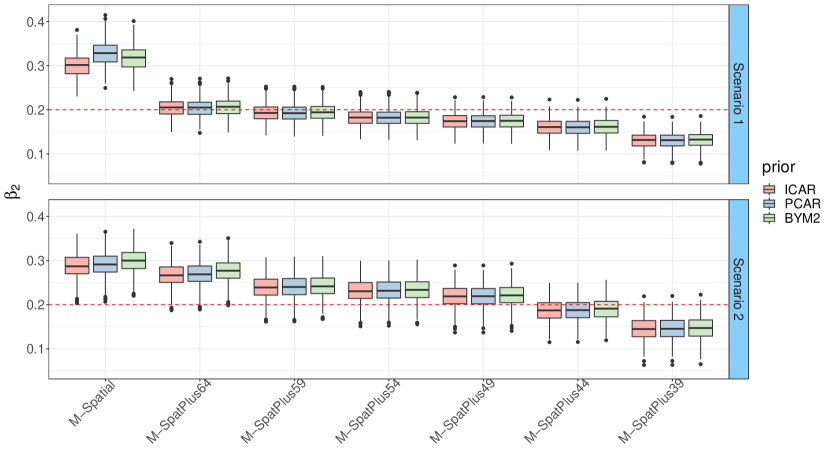
Tables 5 and 6 provide the average over the 300 simulated datasets of the posterior means and posterior standard deviations of the regression coefficients and respectively. To visually examine the fixed effect estimates of different models, Figures 4 and 5 display boxplots of the posterior means of and over the 300 simulated datasets for Scenarios 1 and 2 respectively. In general, the M-Spatial model provides highly biased fixed effects estimates whereas some of the M-models with the spatial+ method recover quite well the true values of the regression coefficients. The number of large-scale eigenvectors of that should be omitted in and hence assigned to (see Equation 3) depends on the relationship between the observed and unobserved covariates. In the scenarios addressed here, we contemplate correlations of 0.5 and 0.3 (moderate and low) between sex ratio and the unobserved covariate in crime 1 and correlations of 0.7 and 0.5 (high and moderate) in crime 2. Supplementary material A addresses correlations of 0.5, 0.3 and 0.0 (moderate, low and no correlation) between sex ratio and the unobserved covariate in crime 1 and correlation of 0.7 (high) between sex ratio and the unobserved covariate in crime 2.
| Model | True value | ICAR | PCAR | BYM2 | ||||
| Mean | SD | Mean | SD | Mean | SD | |||
| Scenario 1 | M-Spatial | -0.1500 | -0.2996 | 0.0674 | -0.3162 | 0.0457 | -0.3048 | 0.0534 |
| M-SpatPlus64 | -0.1869 | 0.0446 | -0.1895 | 0.0429 | -0.1942 | 0.0433 | ||
| M-SpatPlus59 | -0.1818 | 0.0419 | -0.1863 | 0.0407 | -0.1932 | 0.0415 | ||
| M-SpatPlus54 | -0.1303 | 0.0407 | -0.1315 | 0.0402 | -0.1332 | 0.0420 | ||
| M-SpatPlus49 | -0.1141 | 0.0399 | -0.1152 | 0.0398 | -0.1162 | 0.0419 | ||
| Scenario 2 | M-Spatial | -0.1500 | -0.2707 | 0.0733 | -0.2619 | 0.0477 | -0.2590 | 0.0579 |
| M-SpatPlus64 | -0.1692 | 0.0481 | -0.1710 | 0.0449 | -0.1746 | 0.0452 | ||
| M-SpatPlus59 | -0.1648 | 0.0453 | -0.1695 | 0.0431 | -0.1748 | 0.0440 | ||
| M-SpatPlus54 | -0.1209 | 0.0431 | -0.1208 | 0.0422 | -0.1211 | 0.0443 | ||
| M-SpatPlus49 | -0.1096 | 0.0419 | -0.1110 | 0.0416 | -0.1109 | 0.0442 | ||
| Model | True value | ICAR | PCAR | BYM2 | ||||
| Mean | SD | Mean | SD | Mean | SD | |||
| Scenario 1 | M-Spatial | -0.2000 | -0.3828 | 0.0596 | -0.4140 | 0.0407 | -0.3996 | 0.0462 |
| M-SpatPlus64 | -0.2258 | 0.0429 | -0.2253 | 0.0454 | -0.2282 | 0.0438 | ||
| M-SpatPlus59 | -0.2094 | 0.0408 | -0.2075 | 0.0432 | -0.2143 | 0.0423 | ||
| M-SpatPlus54 | -0.1663 | 0.0396 | -0.1655 | 0.0421 | -0.1677 | 0.0424 | ||
| M-SpatPlus49 | -0.1412 | 0.0393 | -0.1400 | 0.0417 | -0.1410 | 0.0426 | ||
| Scenario 2 | M-Spatial | -0.2000 | -0.3152 | 0.0690 | -0.3556 | 0.0443 | -0.3403 | 0.0508 |
| M-SpatPlus64 | -0.1881 | 0.0465 | -0.1885 | 0.0477 | -0.1922 | 0.0459 | ||
| M-SpatPlus59 | -0.1779 | 0.0438 | -0.1764 | 0.0452 | -0.1857 | 0.0443 | ||
| M-SpatPlus54 | -0.1368 | 0.0418 | -0.1369 | 0.0439 | -0.1403 | 0.0445 | ||
| M-SpatPlus49 | -0.1130 | 0.0411 | -0.1116 | 0.0434 | -0.1132 | 0.0447 | ||
In summary, when the correlation between and unobserved covariates becomes smaller, lower number of eigenvectors should be omitted in . If too many eigenvectors are excluded from , the M-models with the spatial+ provide biased fixed effects. Nevertheless, in the case of crime 1, a greater number of large-scale eigenvectors should be excluded from compared to crime 2. This discrepancy could be explained because the number of counts for crime 1 is smaller than for crime 2. The M-models with the spatial+ approach provide the same fixed effects estimates irrespective of the prior (ICAR, PCAR or BYM2) given to the spatial random effects. For the M-Spatial model, slight differences are observed in the mean estimates depending on the prior chosen.
Examining Tables 5 and 6 we see that the M-SpatPlus models provide smaller posterior standard deviations than the M-Spatial model. The reduction is about 30%. However, drawing a definitive conclusion regarding whether the posterior standard deviation accurately measures the variability of the fixed effect estimates based on this information is not straightforward. Table A.3 and A.4 in Supplementary material A provide the true simulated standard error () and estimated standard error () for and computed as and for . Here is the posterior mean of estimated in simulation and is the average of all the posterior mean estimates across the simulations. Finally, is the posterior standard deviation of in simulation . Overestimation of the standard error occurs when the estimated standard error exceeds the simulated standard error. Conversely, if the estimated standard error is lower than the simulated standard error, it results in an underestimation of the standard error of the fixed effects. Here, both the M-Spatial and the M-SpatPlus models tend to overestimate the standard error of the fixed effects.
To complete the information about fixed effects, Table 7 provides the empirical coverage of credible intervals at 95% nominal value for and . In general, the empirical coverages of and are relatively low when using the M-Spatial model. This can be attributed to the large bias introduced by the method. On the contrary, the M-models with the spatial+ approach that remove an appropriate number of eigenvectors exhibit credible intervals with certain overcoverage. This could be explained because the spatial+ approach reduces bias but still inflates the variance. If too many eigenvectors are removed, the coverage is poor because the bias increases.
| Model | |||||||
| ICAR | PCAR | BYM2 | ICAR | PCAR | BYM2 | ||
| Scenario 1 | M-Spatial | 35.6667 | 0.0000 | 5.6667 | 3.0000 | 0.0000 | 0.0000 |
| M-SpatPlus64 | 96.3333 | 94.6667 | 93.0000 | 98.0000 | 98.6667 | 98.6667 | |
| M-SpatPlus59 | 96.3333 | 95.3333 | 93.6667 | 99.0000 | 100.0000 | 99.0000 | |
| M-SpatPlus54 | 97.6667 | 98.3333 | 100.0000 | 96.3333 | 97.3333 | 97.0000 | |
| M-SpatPlus49 | 95.6667 | 95.6667 | 96.6667 | 77.3333 | 80.3333 | 85.6667 | |
| Scenario 2 | M-Spatial | 72.6667 | 26.6667 | 53.3333 | 70.0000 | 0.6667 | 9.6667 |
| M-SpatPlus64 | 99.0000 | 98.6667 | 98.6667 | 100.0000 | 100.0000 | 100.0000 | |
| M-SpatPlus59 | 99.6667 | 99.0000 | 98.6667 | 99.3333 | 99.6667 | 100.0000 | |
| M-SpatPlus54 | 98.3333 | 97.6667 | 99.3333 | 75.6667 | 84.0000 | 88.6667 | |
| M-SpatPlus49 | 95.0000 | 95.3333 | 97.0000 | 42.3333 | 47.0000 | 52.3333 | |
Table 8 displays the average over the simulated data sets of the posterior medians and 95% credible intervals of the between crime correlation in each scenario. Here, we contemplate correlations of 0.7 (Scenario 1) and 0.3 (Scenario 2) between the unobserved covariates and . In both scenarios, the results vary depending on the model and the prior chosen. In general, higher correlations between crimes are estimated when the BYM2 prior is assigned to the spatial random effects. When a high number of large-scale eigenvectors are excluded from the observed covariate, the M-SpatPlus models exhibit higher correlations between crimes. This probably occurs because the spatial dependence removed from the covariate is accounted for by the spatial effects. As a result, the spatial patterns of both crimes may become more similar, potentially leading to an increased correlation between the two crimes. Moreover, the correlation between crimes estimated with the M-models depends on the correlation between and defined in the data generating model. Overall, the estimated between-crime correlations are close to the correlations between and . It is worth noting that the M-models with the spatial+ approach and the BYM2 prior tend to overestimate the correlations. Finally, when the correlation is low, the credible intervals are wider.
| Model | ICAR | PCAR | BYM2 | |||||||
| Median | CI | Median | CI | Median | CI | |||||
| Scenario 1 | M-Spatial | 0.7287 | 0.3607 | 0.9305 | 0.6256 | 0.2464 | 0.8739 | 0.5857 | 0.1678 | 0.8694 |
| M-SpatPlus64 | 0.7277 | 0.4032 | 0.9191 | 0.6313 | 0.3150 | 0.8598 | 0.8099 | 0.5331 | 0.9439 | |
| M-SpatPlus59 | 0.7229 | 0.3931 | 0.9178 | 0.6237 | 0.3140 | 0.8541 | 0.8164 | 0.5461 | 0.9459 | |
| M-SpatPlus54 | 0.7830 | 0.5067 | 0.9380 | 0.6852 | 0.3879 | 0.8868 | 0.8691 | 0.6472 | 0.9631 | |
| M-SpatPlus49 | 0.7958 | 0.5360 | 0.9410 | 0.7045 | 0.4168 | 0.8942 | 0.8808 | 0.6749 | 0.9664 | |
| Scenario 2 | M-Spatial | 0.1535 | -0.2631 | 0.5401 | 0.1710 | -0.2115 | 0.5273 | 0.2759 | -0.2240 | 0.6615 |
| M-SpatPlus64 | 0.2138 | -0.1782 | 0.5729 | 0.2325 | 0.0381 | 0.4566 | 0.6084 | 0.2456 | 0.8345 | |
| M-SpatPlus59 | 0.1989 | -0.1966 | 0.5643 | 0.2194 | 0.0362 | 0.4368 | 0.5921 | 0.2223 | 0.8228 | |
| M-SpatPlus54 | 0.3065 | -0.0621 | 0.6327 | 0.3038 | 0.0830 | 0.5458 | 0.7018 | 0.3673 | 0.8864 | |
| M-SpatPlus49 | 0.3371 | -0.0224 | 0.6506 | 0.3378 | 0.0963 | 0.5970 | 0.7243 | 0.4087 | 0.8919 | |
To conclude the simulation study, we look at model selection criteria and the relative risks estimates. According to Table 9, these criteria do not clearly select any model, though models with the BYM2 prior present slightly lower values, particularly if we compare it with the ICAR prior. Table A.8 in Supplementary material A provides MARB and MRRMSE of the relative risks. M-Spatial and M-SpatPlus models perform similarly in terms of the relative risks estimates and differences between spatial priors are negligible.
| Model | ICAR | PCAR | BYM2 | ||||
| DIC | WAIC | DIC | WAIC | DIC | WAIC | ||
| Scenario 1 | M-Spatial | 946.0498 | 952.7725 | 939.1256 | 937.2348 | 934.8325 | 930.7239 |
| M-SpatPlus64 | 944.8425 | 947.5755 | 941.3371 | 937.9480 | 937.8670 | 930.4969 | |
| M-SpatPlus59 | 945.1169 | 947.9748 | 941.2409 | 937.7502 | 937.9337 | 930.6553 | |
| M-SpatPlus54 | 945.8632 | 947.4914 | 942.4370 | 937.5271 | 940.5496 | 932.8373 | |
| M-SpatPlus49 | 946.5776 | 947.8275 | 943.0707 | 937.6770 | 941.4065 | 933.3797 | |
| Scenario 2 | M-Spatial | 961.6077 | 962.9980 | 953.7916 | 946.1904 | 949.2563 | 939.0299 |
| M-SpatPlus64 | 960.3800 | 958.9302 | 953.9252 | 945.8736 | 950.2834 | 937.4415 | |
| M-SpatPlus59 | 960.3221 | 959.2081 | 953.7474 | 946.2881 | 949.9048 | 937.1384 | |
| M-SpatPlus54 | 960.7991 | 957.1269 | 954.7606 | 944.6926 | 952.5815 | 938.9499 | |
| M-SpatPlus49 | 961.0325 | 956.6160 | 955.0791 | 944.1604 | 953.0834 | 939.0144 | |
6.2 Simulation study 2: Results
The primary objective of this second simulation study is to evaluate how well the proposed multivariate models estimate the correlations between crimes and the fixed effects. In the data simulation, the dependence between crimes is introduced by the covariance matrix where defines the correlation between the spatial patterns of crime 1 and crime 2. Hence, we will compare the estimated correlations with the true used in the data generating process. Moreover, we will also examine the fixed effect estimates as in Simulation Study 1.
| Model | ICAR | PCAR | BYM2 | |||||||
| Median | CI | Median | CI | Median | CI | |||||
| Scenario 1 () | M-Spatial | 0.6991 | 0.4669 | 0.8547 | 0.6825 | 0.4611 | 0.8404 | 0.7328 | 0.4952 | 0.8854 |
| M-SpatPlus64 | 0.6951 | 0.4738 | 0.8456 | 0.6889 | 0.4795 | 0.8359 | 0.7184 | 0.4928 | 0.8664 | |
| M-SpatPlus59 | 0.6783 | 0.4499 | 0.8347 | 0.6745 | 0.4624 | 0.8264 | 0.7008 | 0.4718 | 0.8543 | |
| M-SpatPlus54 | 0.6954 | 0.4775 | 0.8438 | 0.6883 | 0.4841 | 0.8338 | 0.7177 | 0.4954 | 0.8642 | |
| M-SpatPlus49 | 0.7062 | 0.4926 | 0.8516 | 0.6977 | 0.4996 | 0.8379 | 0.7271 | 0.5102 | 0.8698 | |
| M-SpatPlus44 | 0.7192 | 0.5137 | 0.8586 | 0.7081 | 0.5116 | 0.8467 | 0.7398 | 0.5326 | 0.8752 | |
| M-SpatPlus39 | 0.7221 | 0.5197 | 0.8599 | 0.7086 | 0.5148 | 0.8462 | 0.7454 | 0.5369 | 0.8806 | |
| Scenario 2 () | M-Spatial | 0.4529 | 0.1511 | 0.6942 | 0.3180 | 0.0074 | 0.6090 | 0.5037 | 0.1921 | 0.7490 |
| M-SpatPlus64 | 0.4873 | 0.1998 | 0.7148 | 0.3865 | 0.1048 | 0.6429 | 0.5533 | 0.2664 | 0.7764 | |
| M-SpatPlus59 | 0.5058 | 0.2339 | 0.7195 | 0.4128 | 0.1378 | 0.6579 | 0.5699 | 0.2971 | 0.7799 | |
| M-SpatPlus54 | 0.4969 | 0.2232 | 0.7131 | 0.4042 | 0.1293 | 0.6528 | 0.5596 | 0.2856 | 0.7728 | |
| M-SpatPlus49 | 0.5155 | 0.2469 | 0.7254 | 0.4233 | 0.1469 | 0.6687 | 0.5761 | 0.3092 | 0.7808 | |
| M-SpatPlus44 | 0.5439 | 0.2913 | 0.7417 | 0.4510 | 0.1761 | 0.6892 | 0.6068 | 0.3498 | 0.7997 | |
| M-SpatPlus39 | 0.5588 | 0.3129 | 0.7501 | 0.4629 | 0.1801 | 0.7040 | 0.6226 | 0.3742 | 0.8097 | |
Table 10 displays the averages over the simulated data sets of the posterior median and 95% credible intervals of the between-crime correlations in each scenario. Here, the data generating process assumes (Scenario 1), (Scenario 2), that is, high and low correlations between the spatial patterns of the crimes. For the high correlation scenario, all the M-models effectively capture , but for low correlation, is overestimated. Indeed, in line with the Simulation Study 1 for the low correlation scenario, the estimates of increase in the M-SpatPlus models as more large-scale eigenvectors are removed. Additionaly, unlike in Simulation Study 1, the correlation parameter is significant as the credible intervals are not too wide. This is probably because the generating model is the same as the fitted model. Supplementary material B examines a scenario (Scenario 3) in which the data generating model assumes a moderate correlation between the spatial patterns. In this case, the estimated correlation coefficient is also overestimated (See Table B.12). In general, the overestimation of is larger with the BYM2 prior than with the ICAR and PCAR priors.
| Model | True value | ICAR | PCAR | BYM2 | ||||
| Mean | SD | Mean | SD | Mean | SD | |||
| Scenario 1 | M-Spatial | 0.1500 | 0.2701 | 0.0815 | 0.2766 | 0.0837 | 0.2760 | 0.0846 |
| M-SpatPlus64 | 0.1878 | 0.0612 | 0.1871 | 0.0619 | 0.1895 | 0.0630 | ||
| M-SpatPlus59 | 0.1914 | 0.0585 | 0.1915 | 0.0593 | 0.1961 | 0.0605 | ||
| M-SpatPlus54 | 0.1709 | 0.0580 | 0.1705 | 0.0587 | 0.1731 | 0.0599 | ||
| M-SpatPlus49 | 0.1580 | 0.0563 | 0.1579 | 0.0571 | 0.1600 | 0.0584 | ||
| M-SpatPlus44 | 0.1405 | 0.0547 | 0.1407 | 0.0555 | 0.1425 | 0.0574 | ||
| M-SpatPlus39 | 0.1260 | 0.0517 | 0.1260 | 0.0526 | 0.1289 | 0.0549 | ||
| Scenario 2 | M-Spatial | 0.1500 | 0.2688 | 0.0685 | 0.2726 | 0.0712 | 0.2733 | 0.0708 |
| M-SpatPlus64 | 0.2406 | 0.0656 | 0.2400 | 0.0681 | 0.2407 | 0.0675 | ||
| M-SpatPlus59 | 0.2160 | 0.0640 | 0.2140 | 0.0665 | 0.2140 | 0.0656 | ||
| M-SpatPlus54 | 0.2173 | 0.0625 | 0.2157 | 0.0650 | 0.2164 | 0.0642 | ||
| M-SpatPlus49 | 0.1996 | 0.0612 | 0.1982 | 0.0636 | 0.1985 | 0.0631 | ||
| M-SpatPlus44 | 0.1700 | 0.0599 | 0.1685 | 0.0624 | 0.1683 | 0.0624 | ||
| M-SpatPlus39 | 0.1454 | 0.0567 | 0.1445 | 0.0593 | 0.1441 | 0.0599 | ||
| Model | True value | ICAR | PCAR | BYM2 | ||||
| Mean | SD | Mean | SD | Mean | SD | |||
| Scenario 1 | M-Spatial | 0.2000 | 0.3018 | 0.0476 | 0.3284 | 0.0519 | 0.3179 | 0.0501 |
| M-SpatPlus64 | 0.2055 | 0.0380 | 0.2051 | 0.0404 | 0.2069 | 0.0398 | ||
| M-SpatPlus59 | 0.1938 | 0.0370 | 0.1935 | 0.0393 | 0.1947 | 0.0388 | ||
| M-SpatPlus54 | 0.1829 | 0.0367 | 0.1829 | 0.0390 | 0.1830 | 0.0385 | ||
| M-SpatPlus49 | 0.1741 | 0.0355 | 0.1739 | 0.0378 | 0.1745 | 0.0374 | ||
| M-SpatPlus44 | 0.1605 | 0.0353 | 0.1599 | 0.0375 | 0.1613 | 0.0375 | ||
| M-SpatPlus39 | 0.1304 | 0.0341 | 0.1302 | 0.0364 | 0.1312 | 0.0367 | ||
| Scenario 2 | M-Spatial | 0.2000 | 0.2876 | 0.0381 | 0.2914 | 0.0393 | 0.2997 | 0.0399 |
| M-SpatPlus64 | 0.2674 | 0.0371 | 0.2694 | 0.0382 | 0.2771 | 0.0392 | ||
| M-SpatPlus59 | 0.2394 | 0.0380 | 0.2403 | 0.0389 | 0.2423 | 0.0401 | ||
| M-SpatPlus54 | 0.2314 | 0.0374 | 0.2323 | 0.0383 | 0.2337 | 0.0395 | ||
| M-SpatPlus49 | 0.2189 | 0.0368 | 0.2190 | 0.0376 | 0.2213 | 0.0389 | ||
| M-SpatPlus44 | 0.1876 | 0.0378 | 0.1880 | 0.0384 | 0.1905 | 0.0404 | ||
| M-SpatPlus39 | 0.1454 | 0.0373 | 0.1458 | 0.0379 | 0.1472 | 0.0404 | ||
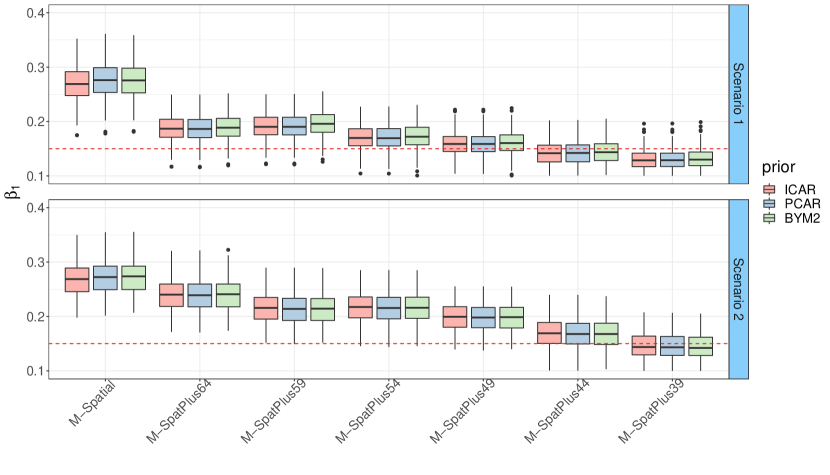
Regarding the fixed effects, Table 11 and Table 12 show the average over the 300 simulated datasets of the posterior means and posterior standard deviations of the regression coefficients (crime 1) and (crime 2) in Scenarios 1 and 2 respectively. Figures 6 and 7 provide the boxplots of the posterior means of and over the 300 simulated data sets. Looking at these tables and figures, some differences can be observed compared to Simulation Study 1. Here, in the M-SpatPlus models, the number of eigenvectors that must be omitted from the observed covariate to recover the fixed effects does not appear to depend on the linear correlation between and the spatial effects used in the data generating model, but rather on the spatial pattern of the covariate. The covariate and both spatial patterns of Scenario 1 have quite similar structure: the values of the districts in the northwest are low, and as we move to the middle southeast districts, the values gradually increase. Conversely, in Scenario 2 the structures are more complex. The spatial patterns show contrasting directions, and somehow a combination of both spatial patterns can be observed in . In the high correlation scenario (Scenario 1), removing 20 large-scale eigenvectors from the covariate seems enough to recover (see Table 11) and between 5 to 15 eigenvectors for (see Table 12). For crime 2, fewer eigenvectors are likely sufficient, possibly due to the larger number of simulated counts. In contrast, when examining the low correlation scenario (Scenario 2), the removal of 20 large-scale eigenvectors in the M-SpatPlus models leads to an overestimation of the fixed effects, particularly for crime 1 (see Table 11). To address this issue, we have fitted the M-SpatPlus model removing more eigenvectors from the covariate. Specifically, we have remove 25 and 30 large-scale eigenvectors (M-SpatPlus44 and M-SpatPlus39 respectively in the tables). Interestingly, when 30 large-scale eigenvectors were removed, the M-SpatPlus estimates of are satisfactory. There are no considerable differences between the ICAR, PCAR and BYM2 priors in terms of the fixed effect estimates.
Similarly to Simulation Study 1, we have compared the true simulated standard error () and the estimated standard error () for and (see Tables B.15 and B.16 of the Supplementary material B) and we provide the empirical coverage of credible intervals at 95% nominal value for and (Table 13). The overestimation of the standard deviations of is quite apparent (see Table B.15). The estimated standard deviation is approximately three times the simulated estandard error. This overestimation is reflected in the 95% coverage probabilities of M-SpatPlus, where nearly all the methods lead to an overcoverage. The reason is that the M-SpatialPlus models reduce bias, but still the variance seems inflated, hence the excess of coverage. In the case of the overestimation of the standard deviations is lower (see Table B.16) and more reasonable 95% coverage probabilities are obtained for the M-SpatPlus models. As in Simulation Study 1, the empirical coverage of and with the usual multivariate M-Spatial model is low because the overestimation of the standard deviation does not compensate for the large bias.
To finish, we examine model selection criteria and MARB and MRRMSE of the relative risks estimates. Table 14 provides the DIC and WAIC for Scenarios 1 and 2. Again, model selection criteria do not effectively differentiate between the models and spatial priors. Table B.19 provides MARB and MRRMSE of the relative risks. All the M-models have similar bias and error concerning the relative risks estimates.
| Model | |||||||
| ICAR | PCAR | BYM2 | ICAR | PCAR | BYM2 | ||
| Scenario 1 | M-Spatial | 86.0000 | 84.6667 | 85.0000 | 40.3333 | 19.6667 | 25.3333 |
| M-SpatPlus64 | 100.0000 | 100.0000 | 100.0000 | 100.0000 | 100.0000 | 100.0000 | |
| M-SpatPlus59 | 100.0000 | 100.0000 | 100.0000 | 100.0000 | 100.0000 | 100.0000 | |
| M-SpatPlus54 | 100.0000 | 100.0000 | 100.0000 | 100.0000 | 100.0000 | 100.0000 | |
| M-SpatPlus49 | 100.0000 | 100.0000 | 100.0000 | 99.3333 | 99.3333 | 99.3333 | |
| M-SpatPlus44 | 100.0000 | 100.0000 | 100.0000 | 92.3333 | 95.3333 | 95.6667 | |
| M-SpatPlus39 | 100.0000 | 100.0000 | 100.0000 | 47.0000 | 57.6667 | 61.0000 | |
| Scenario 2 | M-Spatial | 70.0000 | 70.6667 | 69.3333 | 31.6667 | 28.0000 | 20.6667 |
| M-SpatPlus64 | 91.0000 | 92.6667 | 92.6667 | 57.3333 | 56.6667 | 51.0000 | |
| M-SpatPlus59 | 98.6667 | 99.0000 | 99.0000 | 91.6667 | 91.3333 | 92.3333 | |
| M-SpatPlus54 | 98.3333 | 99.0000 | 99.0000 | 95.0000 | 95.0000 | 95.3333 | |
| M-SpatPlus49 | 100.0000 | 100.0000 | 100.0000 | 98.3333 | 98.6667 | 98.6667 | |
| M-SpatPlus44 | 100.0000 | 100.0000 | 100.0000 | 99.0000 | 99.3333 | 99.6667 | |
| M-SpatPlus39 | 100.0000 | 100.0000 | 100.0000 | 76.3333 | 77.6667 | 87.0000 | |
| Model | ICAR | PCAR | BYM2 | ||||
| DIC | WAIC | DIC | WAIC | DIC | WAIC | ||
| Scenario 1 | M-Spatial | 966.1754 | 951.4779 | 967.5752 | 950.1012 | 967.0064 | 948.7606 |
| M-SpatPlus64 | 966.8528 | 949.4872 | 967.9400 | 948.4048 | 967.9372 | 947.5738 | |
| M-SpatPlus59 | 967.6719 | 950.0178 | 968.8122 | 949.0177 | 968.8697 | 948.4177 | |
| M-SpatPlus54 | 967.8177 | 949.9382 | 968.9508 | 948.8622 | 969.1185 | 948.4952 | |
| M-SpatPlus49 | 968.4432 | 950.9564 | 969.5225 | 949.7588 | 969.7227 | 949.5140 | |
| M-SpatPlus44 | 969.1746 | 951.9225 | 970.1753 | 950.5237 | 970.4424 | 950.4116 | |
| M-SpatPlus39 | 971.8599 | 955.0197 | 972.7043 | 953.2348 | 973.0639 | 953.3253 | |
| Scenario 2 | M-Spatial | 969.8757 | 952.8217 | 970.7773 | 949.9615 | 970.5796 | 949.5215 |
| M-SpatPlus64 | 969.9933 | 952.1133 | 970.6760 | 949.0728 | 970.6719 | 948.8739 | |
| M-SpatPlus59 | 971.2157 | 951.1453 | 972.0652 | 948.4785 | 972.2841 | 948.9999 | |
| M-SpatPlus54 | 971.8931 | 951.8211 | 972.7483 | 949.2491 | 973.0684 | 949.9883 | |
| M-SpatPlus49 | 973.0603 | 953.3003 | 973.8526 | 950.6847 | 974.2231 | 951.4681 | |
| M-SpatPlus44 | 975.0822 | 954.8057 | 975.8658 | 952.0949 | 976.2864 | 952.9832 | |
| M-SpatPlus39 | 978.8893 | 959.4039 | 979.5481 | 956.4251 | 979.9821 | 957.2993 | |
7 Discussion
The inclusion of the covariates in spatial models, whether they are univariate or multivariate, faces the well known problem of spatial confounding, that is, the impossibility of disentangling the fixed effects and the spatial random effects. A correct estimation of the fixed effects is crucial to gain knowledge about complex diseases like cancer or intricate socio-demographic phenomena, such as crimes against women in India.
To deal with spatial confounding, different methods have been proposed in the literature, but we focus on the spatial+ approach as it has proven to work well at least in univariate spatial models. In this paper we propose a modified and simpler version of the method that avoids fitting a spatial model to the covariate. Here, the covariate is expressed as a linear combination of eigenvectors of the spatial precision matrix, and from this linear combination we discard a pre-determined number of large-scale eigenvectors which we assume to be the spatially confounded part of the covariate. With this modified spatial+ approach we avoid fitting a model to the covariate and we directly consider a “spatially decorrelated” version of it. The method can be used in univariate as well as in multivariate models, but in this work we focus on the latter. The method is simple and flexible, allowing for the removal of spatial structure from the covariate differently for each of the response variables.
To illustrate the proposal, two crimes against women, namely rapes and dowry deaths, are analysed jointly in the 70 districts of Uttar Pradesh in 2011. In particular, we have focused on the linear association between the covariate sex ratio and the crimes. All the multivariate models indicate that there is no significant linear association between sex ratio and rapes, whereas for dowry deaths the strength of the association depends on the number of removed eigenvectors from the covariate. Additionally, all the models estimate a rather low positive correlation between rapes and dowry deaths that is on the verge of statistical significance. Our proposal requires consideration about the number of eigenvectors to remove from the linear combination of the covariate. To provide some guidelines, we have conducted two simulation studies. In Simulation Study 1, spatial confounding is induced including two covariates in the data generating model for each crime. Namely, the sex ratio () for both crimes, for crime 1 and for crime 2. The covariates and play the role of unobserved covariates (they are replaced by spatial random effects in the fit) and are correlated, hence they induce dependence between crimes. In Simulation study 2, we have generated the spatial effects and for crimes 1 and 2 respectively from a multivariate ICAR prior with fixed correlation parameter. These spatial effects are responsible for causing correlation between crimes. Then, the observed covariate , is simulated to be correlated with both the spatial effects, and , and different scenarios are simulated depending on the correlations between the covariates and the spatial effects. Overall, the findings of the simulation studies are interesting. The M-models with the original covariate without the spatial+ method do not recover the true fixed effects in any of the simulated scenarios. This is particularly striking in Scenario 2 where the multivariate ICAR is the data generating model. On the contrary, M-models with the spatial+ method provide fairly unbiased estimates and the estimates do not depend on the prior given to the spatial random effects. The key lies in determining beforehand the amount of spatial dependence that we should remove from the covariate. In Simulation Study 1, where the observed covariate (sex ratio) has a clear and gradual spatial pattern, the greater the correlation between the observed and the unobserved covariates, the larger the number of eigenvectors to remove. To be more specific, we should remove between 7% and 20% of the eigenvectors corresponding to the lowest eigenvalues. It is worth noting that in crime 1 we have to remove more eigenvectors than in crime 2, probably because the number of counts is smaller.
In Simulation study 2, results are revealing. It seems that the number of eigenvectors to remove depends more on the spatial dependence of the observed covariate than on the correlation between the observed and unobserved parts of the model. In scenario 1, where the spatial pattern of the simulated observed covariate is more or less smooth and the correlation with the unobserved part is moderate-high, we need to remove about of the eigenvectors in crime 1 and between and of the eigenvectors for crime 2. In scenario 2, where the spatial pattern of the covariate is not so smooth and the correlation with the unobserved part is low-moderate, we need to remove between and of the eigenvectors (this seems to be in line with recent results about confounding at high frequencies by Dupont et al.,, 2023). As in Simulation Study 1, we need to remove more eigenvectors in crime 1 than in crime 2.
To sum up, if the spatial pattern of the observed covariate is smooth, removing to of the eigenvectors should be a good choice. If the spatial pattern of the covariate is not so smooth, then we should remove to eigenvectors. We find these guidelines useful as they depend on the observed covariate rather than on the unobserved ones.
In terms of the between-crime correlation estimates, all models recover quite well high correlations, though low-moderate correlations might be overestimated. Moreover, the overestimation is larger if we remove more eigenvectors than needed. Additionally, the overestimation is larger with the BYM2 spatial prior.
The multivariate models employing the spatial+ approach address bias in the estimates of fixed effects. However, there seems to be an issue with inflated standard errors, leading to overcoverage of the credible intervals. Further research is necessary to adequately adjust the standard errors. Additionally, model selection criteria such as DIC or WAIC do not differentiate between the models. This is somewhat expected, considering that the spatial+ approach can be seen as a reparameterized spatial model.
Finally, it is worth noting that the proposed modified spatial+ approach is valid for univariate and multivariate models. In general we do not expect big differences in the estimation of the fixed effects in univariate and multivariate models if a true relationship between the responses and the covariate exists. However, we think that in complex phenomena such as crimes against women (or cancer, where risk factors only explain a small percentage of cases) multivariate models are more convenient to deal with the problem as a whole and not with each part individually.
Declaration of competing interest
The authors declare that they have no known competing financial interests or personal relationship that could have appeared to influence the work reported in this paper.
Acknowledgements
This work has been supported by Project PID2020-113125RB-I00/MCIN/AEI/10.13039/501100011033. We extend our gratitude to the Associate Editor and the reviewer for their insightful comments, which greatly contributed to enhancing the final version of this article.
A Appendix
A.1 Appendix A
In this Appendix we show that choosing the Cholesky square root of the between-crime covariance matrix has effects that are not independent of the column ordering of , that is, the crime ordering in the analysis.
Consider , the real case study in this work. If is any nonsingular matrix that satisfies the condition , then the corresponding covariance matrix of is
| (A.1) | |||||
| (A.4) |
If we want to choose to be the Cholesky square root, we need to impose the restriction , and then . However, the effect of the restriction is not independent of the crime ordering because for , the restriction implies cross-covariances that only depend on , whereas if we interchange the order, that is, cross-covariances depend only on . To avoid this dependence on the crime ordering, rather than defining as the Cholesky square root of , we allow it to vary more freely although we use the Bartlett decomposition to avoid overparameterization as outlined in Section 4.
A.2 Appendix B
Here we show that the precision parameters are fixed at 1 (or ) for identifiability issues. We remark that for identifiability issues we refer to the situation where there are several unknown quantities but it is impossible to determine each quantity separately because different combinations lead to the same result, that is, the estimation problem does not have a unique solution. Here, given a covariance structure, , the quantities , , and are not identifiable.
In the case of separable covariance structures, the reason to fix the precision parameter (or ) equal to 1 is clear. The within-crime covariance matrix (the inverse of the spatial precision matrix) is the same for all crimes and the global covariance structure is
Then, a change in the scale of can be compensated for by an appropriate change in the scale of .
In the case of non-separable covariance structures, suppose
| (A.5) | |||||
| (A.8) |
for some , and , with . Then, Eq. (A.5) does not have a unique solution. If , and is one solution, then so is any combination , and for which , , , and . One such example is the choice for and , , and .
However, if we fix , then is identifiable as
uniquely determines
Note that setting (i.e. not necessarily equal to 1) only identifies up to scaling. That is, the overall scaling can be done by scaling or scaling . This implies that fixing is not so relevant as looking at Equations (A.1) and (A.5), where the diagonal elements represent the spatial dependence within each crime, the overall smoothing can be controlled by or by the elements of the matrix . Finally, we remark that the matrix is not identifiable (even if ) because there are several choices of square roots for the matrix .
References
- Adin et al., (2023) Adin, A., Goicoa, T., Hodges, J. S., Schnell, P. M., & Ugarte, M. D. (2023). Alleviating confounding in spatio-temporal areal models with an application on crimes against women in India. Statistical Modelling, 23(1), 9–30. https://doi.org/10.1177/1471082X211015452
- Banerjee et al., (2015) Banerjee, S., Carlin, B. P., & Gelfand, A. E. (2015). Hierarchical Modelling and Analysis for Spatial Data, Second Edition. Chapman & Hall, Boca Raton.
- Besag, (1974) Besag, J. (1974). Spatial interaction and the statistical analysis of lattice systems (with discussion). Journal of the Royal Statistical Society: Series B (Statistical Methodology), 36, 192–236. https://doi.org/10.1111/j.2517-6161.1974.tb00999.x
- Botella-Rocamora et al., (2015) Botella-Rocamora, P., Martinez-Beneito, M., & Banerjee, S. (2015). A unifying modeling framework for highly multivariate disease mapping. Statistics in Medicine, 34(9), 1548–1559. https://doi.org/10.1002/sim.6423
- Congdon, (2013) Congdon, P. (2013). Assessing the impact of socioeconomic variables on small area variations in suicide outcomes in england. International Journal of Environmental Research and Public Health, 10(1), 158–177. https://doi.org/10.3390/ijerph10010158
- Dupont et al., (2023) Dupont, E., Marques, I., & Kneib, T. (2023). Demystifying spatial confounding. https://doi.org/10.48550/arXiv.2309.16861
- Dupont et al., (2022) Dupont, E., Wood, S. N., & Augustin, N. H. (2022). Spatial+: A novel approach to spatial confounding. Biometrics, 78(4), 1279–1290. https://doi.org/10.1111/biom.13656
- Gilbert et al., (2022) Gilbert, B., Datta, A., & Ogburn, E. (2022). Approaches to spatial confounding in geostatistics. arXiv:2112.14946v2. https://doi.org/10.48550/arXiv.2112.14946
- Goicoa et al., (2018) Goicoa, T., Adin, A., Ugarte, M. D., & Hodges, J. S. (2018). In spatio-temporal disease mapping models, identifiability constraints affect PQL and INLA results. Stochastic Environmental Research and Risk Assessment, 32(3), 749–770. https://doi.org/10.1007/s00477-017-1405-0
- Guan et al., (2022) Guan, Y., Page, G. L., Reich, B. J., Ventrucci, M., & Yang, S. (2022). Spectral adjustment for spatial confounding. Biometrika, 110(3), 669–719. https://doi.org/10.1093/biomet/asac069
- Hanks et al., (2015) Hanks, E. M., Schliep, E. M., Hooten, M. B., & Hoeting, J. A. (2015). Restricted spatial regression in practice: geostatistical models, confounding, and robustness under model misspecification. Environmetrics, 26(4), 243–254. https://doi.org/10.1002/env.2331
- Harville, (2008) Harville, D. A. (2008). Matrix Algebra from a Statistician’s Perspective. Springer, New York.
- Hodges & Reich, (2010) Hodges, J. S. & Reich, B. J. (2010). Adding spatially-correlated errors can mess up the fixed effect you love. The American Statistician, 64(4), 325–334. https://doi.org/10.1198/tast.2010.10052
- Hughes & Haran, (2013) Hughes, J. & Haran, M. (2013). Dimension reduction and alleviation of confounding for spatial generalized linear mixed models. Journal of the Royal Statistical Society: Series B (Statistical Methodology), 75(1), 139–159. https://doi.org/10.1111/j.1467-9868.2012.01041.x
- Jin et al., (2007) Jin, X., Banerjee, S., & Carlin, B. P. (2007). Order-free co-regionalized areal data models with application to multiple-disease mapping. Journal of the Royal Statistical Society: Series B (Statistical Methodology), 69(5), 817–838. https://doi.org/10.1111/j.1467-9868.2007.00612.x
- Khan & Calder, (2022) Khan, K. & Calder, C. A. (2022). Restricted spatial regression methods: implications for inference. Journal of the American Statistical Association, 117(537), 482–494. https://doi.org/10.1080/01621459.2020.1788949
- Lindgren & Rue, (2015) Lindgren, F. & Rue, H. (2015). Bayesian spatial modelling with r-inla. Journal of Statistical Software, 63(19), 1–25. https://doi.org/10.18637/jss.v063.i19
- MacNab, (2018) MacNab, Y. C. (2018). Some recent work on multivariate Gaussian Markov random fields. Test, 27(3), 497–541. https://doi.org/10.1007/s11749-018-0605-3
- Marques et al., (2022) Marques, I., Kneib, T., & Klein, M. (2022). Mitigating spatial confounding by explicitly correlating gaussian random fields. Environmetrics, 33(5), e2727. https://doi.org/10.1002/env.2727
- Martinez-Beneito, (2013) Martinez-Beneito, M. A. (2013). A general modelling framework for multivariate disease mapping. Biometrika, 100(3), 539–553. https://doi.org/10.1093/biomet/ast023
- Martinez-Beneito & Botella-Rocamora, (2019) Martinez-Beneito, M. A. & Botella-Rocamora, P. (2019). Disease mapping: from foundations to multidimensional modeling. CRC Press, Boca Raton.
- Mukherjee et al., (2001) Mukherjee, C., Rustagi, P., & Krishnaji, N. (2001). Crimes against women in India: Analysis of official statistics. Economic and Political Weekly, 36(43), 4070–4080.
- Page et al., (2017) Page, G. L., Liu, Y., He, Z., & Sun, D. (2017). Estimation and prediction in the presence of spatial confounding for spatial linear models. Scandinavian Journal of Statistics, 44(3), 780–797. https://doi.org/10.1111/sjos.12275
- Peña & Irie, (2022) Peña, V. & Irie, K. (2022). On the Relationship between Uhlig Extended and beta-Bartlett Processes. Journal of Time Series Analysis, 43(1), 147–153. https://doi.org/10.1111/jtsa.12595
- Prates et al., (2015) Prates, M. O., Dey, D. K., Willig, M. R., & Yan, J. (2015). Transformed gaussian markov random fields and spatial modeling of species abundance. Spatial Statistics, 14(PC), 382–399. https://doi.org/10.1016/j.spasta.2015.07.004
- Reich et al., (2006) Reich, B. J., Hodges, J. S., & Zadnik, V. (2006). Effects of residual smoothing on the posterior of the fixed effects in disease-mapping models. Biometrics, 62(4), 1197–1206. https://doi.org/10.1111/j.1541-0420.2006.00617.x
- Riebler et al., (2016) Riebler, A., Sørbye, S. H., Simpson, D., & Rue, H. (2016). An intuitive bayesian spatial model for disease mapping that accounts for scaling. Statistical Methods in Medical Research, 25(4), 1145–1165. https://doi.org/10.1177/0962280216660421
- Rue et al., (2009) Rue, H., Martino, S., & Chopin, N. (2009). Approximate bayesian inference for latent gaussian models by using integrated nested laplace approximations. Journal of the Royal Statistical Society: Series B (Statistical Methodology), 71(2), 319–392. https://doi.org/10.1111/j.1467-9868.2008.00700.x
- Urdangarin et al., (2023) Urdangarin, A., Goicoa, T., & Ugarte, M. D. (2023). Evaluating recent methods to overcome spatial confounding. Revista Complutense Madrid, 36, 333–360. https://doi.org/10.1007/s13163-022-00449-8
- (30) Vicente, G., Adin, A., Goicoa, T., & Ugarte, M. D. (2023a). High-dimensional order-free multivariate spatial disease mapping. Statistics and Computing, 33(104), 1–24. https://doi.org/10.1007/s11222-023-10263-x
- (31) Vicente, G., Goicoa, T., Fernandez-Rasines, P., & Ugarte, M. D. (2020a). Crime Against Women in India: Unveiling Spatial Patterns and Temporal Trends of Dowry Deaths in the Districts of Uttar Pradesh. Journal of the Royal Statistical Society Series A: Statistics in Society, 183(2), 655–679. https://doi.org/10.1111/rssa.12545
- Vicente et al., (2018) Vicente, G., Goicoa, T., Puranik, A., & Ugarte, M. D. (2018). Small area estimation of gender-based violence: rape incidence risks in Uttar Pradesh, India. Statistics and Applications, 16(1), 71–90.
- (33) Vicente, G., Goicoa, T., & Ugarte, M. D. (2020b). Bayesian inference in multivariate spatio-temporal areal models using INLA: analysis of gender-based violence in small areas. Stochastic Environmental Research and Risk Assessment, 34, 1421–1440. https://doi.org/10.1007/s00477-020-01808-x
- (34) Vicente, G., Goicoa, T., & Ugarte, M. D. (2023b). Multivariate Bayesian spatio-temporal P-spline models to analyze crimes against women. Biostatistics, 24(3), 562–584. https://doi.org/10.1093/biostatistics/kxab042
A Supplementary material: Simulation study 1
This section includes some additional scenarios to complement the analysis of Simulation study 1. The data is generated following the generating models (11)-(12) with , , and is the standardized sex ratio covariate. Below we define the correlations between , and chosen in each scenario:
-
•
Scenario 3: , and are chosen. This is similar to Scenario 1 but choosing lower correlation between and .
-
•
Scenario 4: , and are chosen.
-
•
Scenario 5: , and are chosen.
-
•
Scenario 6: , and are chosen.
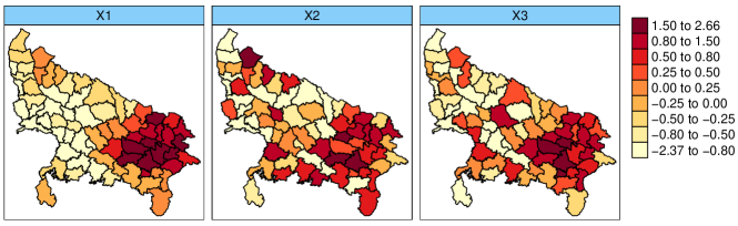
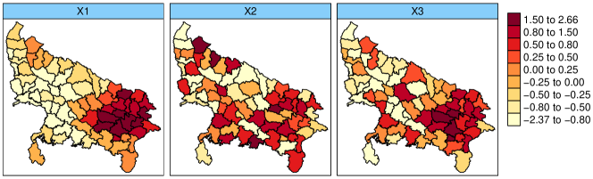
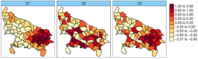
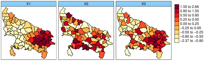
| ICAR | PCAR | BYM2 | ||||||
| Model | True value | Mean | SD | Mean | SD | Mean | SD | |
| Scenario 3 | M-Spatial | -0.1500 | -0.3207 | 0.0684 | -0.3169 | 0.0457 | -0.3130 | 0.0552 |
| M-SpatPlus64 | -0.1988 | 0.0456 | -0.2002 | 0.0423 | -0.2034 | 0.0432 | ||
| M-SpatPlus59 | -0.1915 | 0.0430 | -0.1951 | 0.0406 | -0.1995 | 0.0417 | ||
| M-SpatPlus54 | -0.1432 | 0.0416 | -0.1434 | 0.0403 | -0.1439 | 0.0422 | ||
| M-SpatPlus49 | -0.1288 | 0.0407 | -0.1297 | 0.0399 | -0.1301 | 0.0421 | ||
| Scenario 4 | M-Spatial | -0.1500 | -0.2721 | 0.0734 | -0.2604 | 0.0476 | -0.2596 | 0.0583 |
| M-SpatPlus64 | -0.1700 | 0.0482 | -0.1715 | 0.0438 | -0.1742 | 0.0446 | ||
| M-SpatPlus59 | -0.1653 | 0.0454 | -0.1694 | 0.0418 | -0.1740 | 0.0432 | ||
| M-SpatPlus54 | -0.1225 | 0.0430 | -0.1223 | 0.0407 | -0.1222 | 0.0429 | ||
| M-SpatPlus49 | -0.1117 | 0.0418 | -0.1126 | 0.0401 | -0.1125 | 0.0427 | ||
| Scenario 5 | M-Spatial | -0.1500 | -0.1067 | 0.0773 | -0.1598 | 0.0487 | -0.1361 | 0.0567 |
| M-SpatPlus64 | -0.0657 | 0.0489 | -0.0711 | 0.0488 | -0.0772 | 0.0463 | ||
| M-SpatPlus59 | -0.0681 | 0.0461 | -0.0742 | 0.0464 | -0.0853 | 0.0448 | ||
| M-SpatPlus54 | -0.0386 | 0.0421 | -0.0408 | 0.0423 | -0.0447 | 0.0433 | ||
| M-SpatPlus49 | -0.0255 | 0.0407 | -0.0265 | 0.0408 | -0.0280 | 0.0428 | ||
| Scenario 6 | M-Spatial | -0.1500 | -0.1630 | 0.0737 | -0.1711 | 0.0482 | -0.1614 | 0.0580 |
| M-SpatPlus64 | -0.1046 | 0.0476 | -0.1091 | 0.0445 | -0.1130 | 0.0453 | ||
| M-SpatPlus59 | -0.1078 | 0.0447 | -0.1165 | 0.0422 | -0.1232 | 0.0437 | ||
| M-SpatPlus54 | -0.0697 | 0.0417 | -0.0711 | 0.0401 | -0.0725 | 0.0426 | ||
| M-SpatPlus49 | -0.0609 | 0.0404 | -0.0624 | 0.0390 | -0.0630 | 0.0421 | ||
| ICAR | PCAR | BYM2 | ||||||
| Model | True value | Mean | SD | Mean | SD | Mean | SD | |
| Scenario 3 | M-Spatial | -0.2000 | -0.3863 | 0.0593 | -0.4138 | 0.0401 | -0.4029 | 0.0454 |
| M-SpatPlus64 | -0.2299 | 0.0424 | -0.2290 | 0.0442 | -0.2309 | 0.0435 | ||
| M-SpatPlus59 | -0.2137 | 0.0403 | -0.2112 | 0.0421 | -0.2162 | 0.0420 | ||
| M-SpatPlus54 | -0.1693 | 0.0392 | -0.1687 | 0.0417 | -0.1706 | 0.0422 | ||
| M-SpatPlus49 | -0.1446 | 0.0389 | -0.1433 | 0.0414 | -0.1442 | 0.0424 | ||
| Scenario 4 | M-Spatial | -0.2000 | -0.3819 | 0.0597 | -0.4113 | 0.0403 | -0.4001 | 0.0453 |
| M-SpatPlus64 | -0.2272 | 0.0426 | -0.2267 | 0.0452 | -0.2287 | 0.0440 | ||
| M-SpatPlus59 | -0.2121 | 0.0405 | -0.2101 | 0.0430 | -0.2155 | 0.0425 | ||
| M-SpatPlus54 | -0.1669 | 0.0394 | -0.1664 | 0.0423 | -0.1685 | 0.0432 | ||
| M-SpatPlus49 | -0.1419 | 0.0391 | -0.1405 | 0.0420 | -0.1415 | 0.0434 | ||
| Scenario 5 | M-Spatial | -0.2000 | -0.3730 | 0.0607 | -0.4119 | 0.0402 | -0.3939 | 0.0455 |
| M-SpatPlus64 | -0.2206 | 0.0454 | -0.2240 | 0.0477 | -0.2282 | 0.0440 | ||
| M-SpatPlus59 | -0.2033 | 0.0430 | -0.2066 | 0.0456 | -0.2156 | 0.0426 | ||
| M-SpatPlus54 | -0.1614 | 0.0415 | -0.1618 | 0.0443 | -0.1660 | 0.0437 | ||
| M-SpatPlus49 | -0.1360 | 0.0411 | -0.1353 | 0.0439 | -0.1372 | 0.0443 | ||
| Scenario 6 | M-Spatial | -0.2000 | -0.3818 | 0.0590 | -0.4128 | 0.0401 | -0.4005 | 0.0453 |
| M-SpatPlus64 | -0.2253 | 0.0428 | -0.2259 | 0.0461 | -0.2285 | 0.0437 | ||
| M-SpatPlus59 | -0.2089 | 0.0407 | -0.2082 | 0.0438 | -0.2150 | 0.0423 | ||
| M-SpatPlus54 | -0.1655 | 0.0396 | -0.1650 | 0.0432 | -0.1677 | 0.0433 | ||
| M-SpatPlus49 | -0.1394 | 0.0393 | -0.1382 | 0.0430 | -0.1394 | 0.0438 | ||
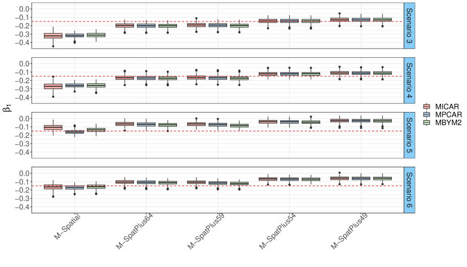
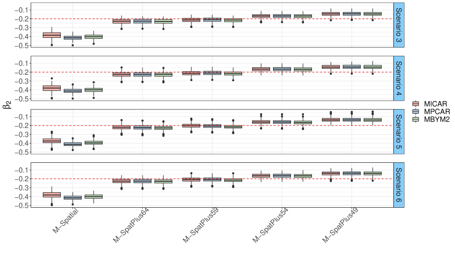
| ICAR | PCAR | BYM2 | |||||
| Model | |||||||
| Scenario 1 | M-Spatial | 0.0674 | 0.0390 | 0.0457 | 0.0263 | 0.0534 | 0.0289 |
| M-SpatPlus64 | 0.0446 | 0.0279 | 0.0429 | 0.0272 | 0.0433 | 0.0267 | |
| M-SpatPlus59 | 0.0419 | 0.0267 | 0.0407 | 0.0261 | 0.0415 | 0.0255 | |
| M-SpatPlus54 | 0.0407 | 0.0264 | 0.0402 | 0.0262 | 0.0420 | 0.0259 | |
| M-SpatPlus49 | 0.0399 | 0.0264 | 0.0398 | 0.0262 | 0.0419 | 0.0262 | |
| Scenario 2 | M-Spatial | 0.0733 | 0.0401 | 0.0477 | 0.0265 | 0.0579 | 0.0307 |
| M-SpatPlus64 | 0.0481 | 0.0275 | 0.0449 | 0.0270 | 0.0452 | 0.0268 | |
| M-SpatPlus59 | 0.0453 | 0.0263 | 0.0431 | 0.0262 | 0.0440 | 0.0257 | |
| M-SpatPlus54 | 0.0431 | 0.0251 | 0.0422 | 0.0252 | 0.0443 | 0.0251 | |
| M-SpatPlus49 | 0.0419 | 0.0246 | 0.0416 | 0.0246 | 0.0442 | 0.0245 | |
| Scenario 3 | M-Spatial | 0.0684 | 0.0419 | 0.0457 | 0.0272 | 0.0552 | 0.0312 |
| M-SpatPlus64 | 0.0456 | 0.0293 | 0.0423 | 0.0287 | 0.0432 | 0.0282 | |
| M-SpatPlus59 | 0.0430 | 0.0280 | 0.0406 | 0.0277 | 0.0417 | 0.0270 | |
| M-SpatPlus54 | 0.0416 | 0.0278 | 0.0403 | 0.0278 | 0.0422 | 0.0277 | |
| M-SpatPlus49 | 0.0407 | 0.0273 | 0.0399 | 0.0273 | 0.0421 | 0.0273 | |
| Scenario 4 | M-Spatial | 0.0734 | 0.0421 | 0.0476 | 0.0259 | 0.0583 | 0.0306 |
| M-SpatPlus64 | 0.0482 | 0.0292 | 0.0438 | 0.0284 | 0.0446 | 0.0280 | |
| M-Spatplus59 | 0.0454 | 0.0285 | 0.0418 | 0.0281 | 0.0432 | 0.0279 | |
| M-SpatPlus54 | 0.0430 | 0.0270 | 0.0407 | 0.0268 | 0.0429 | 0.0271 | |
| M-SpatPlus49 | 0.0418 | 0.0260 | 0.0401 | 0.0257 | 0.0427 | 0.0261 | |
| Scenario 5 | M-Spatial | 0.0773 | 0.0346 | 0.0487 | 0.0252 | 0.0567 | 0.0270 |
| M-SpatPlus64 | 0.0489 | 0.0247 | 0.0488 | 0.0244 | 0.0463 | 0.0237 | |
| M-SpatPlus59 | 0.0461 | 0.0239 | 0.0464 | 0.0237 | 0.0448 | 0.0230 | |
| M-SpatPlus54 | 0.0421 | 0.0229 | 0.0423 | 0.0228 | 0.0433 | 0.0227 | |
| M-SpatPlus49 | 0.0407 | 0.0237 | 0.0408 | 0.0237 | 0.0428 | 0.0237 | |
| Scenario 6 | M-Spatial | 0.0737 | 0.0375 | 0.0482 | 0.0267 | 0.0580 | 0.0287 |
| M-SpatPlus64 | 0.0476 | 0.0258 | 0.0445 | 0.0251 | 0.0453 | 0.0247 | |
| M-SpatPlus59 | 0.0447 | 0.0248 | 0.0422 | 0.0245 | 0.0437 | 0.0240 | |
| M-SpatPlus54 | 0.0417 | 0.0231 | 0.0401 | 0.0228 | 0.0426 | 0.0226 | |
| M-SpatPlus49 | 0.0404 | 0.0236 | 0.0390 | 0.0234 | 0.0421 | 0.0234 | |
| ICAR | PCAR | BYM2 | |||||
| Model | |||||||
| Scenario 1 | M-Spatial | 0.0596 | 0.0357 | 0.0407 | 0.0243 | 0.0462 | 0.0262 |
| M-SpatPlus64 | 0.0429 | 0.0268 | 0.0454 | 0.0267 | 0.0438 | 0.0259 | |
| M-SpatPlus59 | 0.0408 | 0.0257 | 0.0432 | 0.0256 | 0.0423 | 0.0248 | |
| M-SpatPlus54 | 0.0396 | 0.0252 | 0.0421 | 0.0252 | 0.0424 | 0.0251 | |
| M-SpatPlus49 | 0.0393 | 0.0242 | 0.0417 | 0.0243 | 0.0426 | 0.0242 | |
| Scenario 2 | M-Spatial | 0.0690 | 0.0382 | 0.0443 | 0.0252 | 0.0508 | 0.0273 |
| M-SpatPlus64 | 0.0465 | 0.0263 | 0.0477 | 0.0256 | 0.0459 | 0.0244 | |
| M-SpatPlus59 | 0.0438 | 0.0252 | 0.0452 | 0.0245 | 0.0443 | 0.0237 | |
| M-SpatPlus54 | 0.0418 | 0.0242 | 0.0439 | 0.0240 | 0.0445 | 0.0236 | |
| M-SpatPlus49 | 0.0411 | 0.0239 | 0.0434 | 0.0239 | 0.0447 | 0.0237 | |
| Scenario 3 | M-Spatial | 0.0593 | 0.0385 | 0.0401 | 0.0265 | 0.0454 | 0.0284 |
| M-SpatPlus64 | 0.0424 | 0.0279 | 0.0442 | 0.0277 | 0.0435 | 0.0271 | |
| M-SpatPlus59 | 0.0403 | 0.0258 | 0.0421 | 0.0256 | 0.0420 | 0.0248 | |
| M-SpatPlus54 | 0.0392 | 0.0248 | 0.0417 | 0.0246 | 0.0422 | 0.0243 | |
| M-SpatPlus49 | 0.0389 | 0.0243 | 0.0414 | 0.0243 | 0.0424 | 0.0242 | |
| Scenario 4 | M-Spatial | 0.0597 | 0.0391 | 0.0403 | 0.0266 | 0.0453 | 0.0286 |
| M-SpatPlus64 | 0.0426 | 0.0280 | 0.0452 | 0.0282 | 0.0440 | 0.0270 | |
| M-SpatPlus59 | 0.0405 | 0.0262 | 0.0430 | 0.0261 | 0.0425 | 0.0250 | |
| M-SpatPlus54 | 0.0394 | 0.0258 | 0.0423 | 0.0259 | 0.0432 | 0.0254 | |
| M-SpatPlus49 | 0.0391 | 0.0247 | 0.0420 | 0.0249 | 0.0434 | 0.0246 | |
| Scenario 5 | M-Spatial | 0.0607 | 0.0354 | 0.0402 | 0.0262 | 0.0455 | 0.0287 |
| M-SpatPlus64 | 0.0454 | 0.0281 | 0.0477 | 0.0278 | 0.0440 | 0.0268 | |
| M-SpatPlus59 | 0.0430 | 0.0262 | 0.0456 | 0.0260 | 0.0426 | 0.0250 | |
| M-SpatPlus54 | 0.0415 | 0.0256 | 0.0443 | 0.0255 | 0.0437 | 0.0252 | |
| M-SpatPlus49 | 0.0411 | 0.0248 | 0.0439 | 0.0248 | 0.0443 | 0.0247 | |
| Scenario 6 | M-Spatial | 0.0590 | 0.0383 | 0.0401 | 0.0264 | 0.0453 | 0.0285 |
| M-SpatPlus64 | 0.0428 | 0.0276 | 0.0461 | 0.0277 | 0.0437 | 0.0266 | |
| M-SpatPlus59 | 0.0407 | 0.0261 | 0.0438 | 0.0263 | 0.0423 | 0.0251 | |
| M-SpatPlus54 | 0.0396 | 0.0253 | 0.0432 | 0.0252 | 0.0433 | 0.0249 | |
| M-SpatPlus49 | 0.0393 | 0.0250 | 0.0430 | 0.0249 | 0.0438 | 0.0249 | |
| Model | ICAR | PCAR | BYM2 | ICAR | PCAR | BYM2 | |
| Scenario 3 | M-Spatial | 19.3333 | 0.0000 | 6.0000 | 5.0000 | 0.0000 | 0.0000 |
| M-SpatPlus64 | 90.6667 | 87.3333 | 87.0000 | 96.0000 | 98.0000 | 97.3333 | |
| M-SpatPlus59 | 94.6667 | 90.0000 | 89.3333 | 98.6667 | 99.3333 | 99.0000 | |
| M-SpatPlus54 | 99.6667 | 99.6667 | 100.0000 | 96.6667 | 97.3333 | 99.0000 | |
| M-SpatPlus49 | 98.3333 | 98.6667 | 99.0000 | 78.0000 | 82.3333 | 86.0000 | |
| Scenario 4 | M-Spatial | 70.6667 | 26.3333 | 56.0000 | 6.0000 | 0.0000 | 0.0000 |
| M-SpatPlus64 | 99.6667 | 98.3333 | 98.3333 | 96.6667 | 97.6667 | 97.3333 | |
| M-SpatPlus59 | 99.6667 | 98.6667 | 98.3333 | 99.6667 | 99.6667 | 99.6667 | |
| M-SpatPlus54 | 98.0000 | 96.6667 | 97.6667 | 94.0000 | 95.3333 | 97.6667 | |
| M-SpatPlus49 | 95.3333 | 95.6667 | 97.0000 | 75.0000 | 79.6667 | 84.6667 | |
| Scenario 5 | M-Spatial | 100.0000 | 100.0000 | 100.0000 | 9.0000 | 0.0000 | 0.0000 |
| M-SpatPlus64 | 64.3333 | 72.6667 | 73.6667 | 98.0000 | 98.3333 | 97.3333 | |
| M-SpatPlus59 | 61.0000 | 72.6667 | 81.6667 | 100.0000 | 100.0000 | 99.3333 | |
| M-SpatPlus54 | 12.0000 | 13.6667 | 20.3333 | 94.3333 | 96.6667 | 98.0000 | |
| M-SpatPlus49 | 2.0000 | 3.0000 | 6.0000 | 76.6667 | 79.6667 | 83.0000 | |
| Scenario 6 | M-Spatial | 100.0000 | 99.3333 | 100.0000 | 6.3333 | 0.0000 | 0.0000 |
| M-SpatPlus64 | 96.0000 | 95.6667 | 98.0000 | 97.6667 | 97.6667 | 98.3333 | |
| M-SpatPlus59 | 96.3333 | 96.6667 | 100.0000 | 99.0000 | 100.0000 | 98.6667 | |
| M-SpatPlus54 | 49.6667 | 49.3333 | 60.0000 | 94.6667 | 97.0000 | 98.0000 | |
| M-SpatPlus49 | 34.0000 | 31.6667 | 42.0000 | 75.3333 | 82.3333 | 85.6667 | |
| ICAR | PCAR | BYM2 | ||||||||
| Model | Median | CI | Median | CI | Median | CI | ||||
| Scenario 3 | M-Spatial | 0.2568 | -0.2346 | 0.6783 | 0.2359 | -0.1913 | 0.6168 | 0.3250 | -0.2218 | 0.7265 |
| M-SpatPlus64 | 0.3574 | -0.0573 | 0.7085 | 0.2969 | 0.0897 | 0.5364 | 0.7132 | 0.4062 | 0.8911 | |
| M-SpatPlus59 | 0.3508 | -0.0646 | 0.7041 | 0.2907 | 0.0839 | 0.5267 | 0.7183 | 0.4157 | 0.8902 | |
| M-SpatPlus54 | 0.4754 | 0.1048 | 0.7708 | 0.4119 | 0.1556 | 0.6710 | 0.8001 | 0.5474 | 0.9283 | |
| M-SpatPlus49 | 0.5076 | 0.1522 | 0.7859 | 0.4444 | 0.1718 | 0.7044 | 0.8170 | 0.5824 | 0.9340 | |
| Scenario 4 | M-Spatial | 0.0977 | -0.3660 | 0.5370 | 0.1147 | -0.3026 | 0.5084 | 0.2039 | -0.3156 | 0.6323 |
| M-SpatPlus64 | 0.1841 | -0.2184 | 0.5602 | 0.1142 | -0.0361 | 0.2907 | 0.5070 | 0.1514 | 0.7525 | |
| M-SpatPlus59 | 0.1716 | -0.2322 | 0.5512 | 0.1096 | -0.0375 | 0.2842 | 0.5073 | 0.1549 | 0.7534 | |
| M-SpatPlus54 | 0.3030 | -0.0723 | 0.6349 | 0.2212 | 0.0377 | 0.4361 | 0.6889 | 0.3719 | 0.8736 | |
| M-SpatPlus49 | 0.3341 | -0.0300 | 0.6511 | 0.2651 | 0.0557 | 0.5018 | 0.7168 | 0.4094 | 0.8884 | |
| Scenario 5 | M-Spatial | 0.9673 | 0.8510 | 0.9956 | 0.9459 | 0.7517 | 0.9947 | 0.9169 | 0.6412 | 0.9838 |
| M-SpatPlus64 | 0.8722 | 0.6981 | 0.9579 | 0.8538 | 0.6599 | 0.9515 | 0.7170 | 0.3678 | 0.9076 | |
| M-SpatPlus59 | 0.8590 | 0.6711 | 0.9531 | 0.8370 | 0.6308 | 0.9461 | 0.6915 | 0.3197 | 0.8990 | |
| M-SpatPlus54 | 0.8760 | 0.7030 | 0.9608 | 0.8519 | 0.6545 | 0.9527 | 0.7632 | 0.4212 | 0.9302 | |
| M-SpatPlus49 | 0.8789 | 0.7100 | 0.9622 | 0.8511 | 0.6530 | 0.9534 | 0.7805 | 0.4544 | 0.9355 | |
| Scenario 6 | M-Spatial | 0.5144 | 0.0786 | 0.8245 | 0.4409 | 0.0438 | 0.7526 | 0.4642 | 0.0033 | 0.7998 |
| M-SpatPlus64 | 0.4467 | 0.0635 | 0.7441 | 0.3093 | 0.0435 | 0.5584 | 0.4428 | 0.0502 | 0.7570 | |
| M-SpatPlus59 | 0.4150 | 0.0252 | 0.7239 | 0.2605 | 0.0115 | 0.5027 | 0.4133 | 0.0361 | 0.7198 | |
| M-SpatPlus54 | 0.5037 | 0.1515 | 0.7727 | 0.3616 | 0.0993 | 0.6140 | 0.5861 | 0.1926 | 0.8397 | |
| M-SpatPlus49 | 0.5133 | 0.1715 | 0.7757 | 0.3696 | 0.1047 | 0.6226 | 0.6180 | 0.2255 | 0.8573 | |
| ICAR | PCAR | BYM2 | |||||
| Model | DIC | WAIC | DIC | WAIC | DIC | WAIC | |
| Scenario 3 | M-Spatial | 953.3899 | 959.0199 | 944.7410 | 940.6010 | 940.0554 | 933.2278 |
| M-SpatPlus64 | 951.5502 | 952.1564 | 945.9650 | 940.6912 | 942.7260 | 932.5063 | |
| M-SpatPlus59 | 951.5871 | 952.2058 | 945.7270 | 940.4662 | 942.6509 | 932.4621 | |
| M-SpatPlus54 | 953.3013 | 951.8469 | 947.7106 | 939.4825 | 946.1554 | 935.1135 | |
| M-SpatPlus49 | 954.0929 | 952.0263 | 948.5981 | 939.6678 | 947.0794 | 935.5887 | |
| Scenario 4 | M-Spatial | 956.4190 | 959.9196 | 948.3138 | 942.5435 | 943.8799 | 935.4106 |
| M-SpatPlus64 | 954.4169 | 952.4786 | 950.0634 | 943.0617 | 946.4975 | 933.8437 | |
| M-SpatPlus59 | 954.4825 | 952.6663 | 949.9523 | 943.3573 | 946.3982 | 933.9363 | |
| M-SpatPlus54 | 956.0888 | 951.8025 | 951.5685 | 941.7616 | 949.9328 | 936.6268 | |
| M-SpatPlus49 | 956.8527 | 951.8008 | 952.1582 | 941.4476 | 950.8215 | 937.1556 | |
| Scenario 5 | M-Spatial | 920.6782 | 918.4245 | 917.5135 | 913.1496 | 914.1673 | 909.6811 |
| SpatPlus64 | 928.7485 | 920.9094 | 931.7151 | 921.7071 | 926.4891 | 913.7202 | |
| SpatPlus59 | 930.9754 | 923.6303 | 933.8990 | 924.3162 | 928.5294 | 916.3151 | |
| SpatPlus54 | 932.7776 | 925.6282 | 936.0239 | 927.1580 | 931.8094 | 920.4459 | |
| SpatPlus49 | 934.4598 | 927.5054 | 937.6879 | 928.9506 | 933.6649 | 922.6290 | |
| Scenario 6 | Spatial | 955.1080 | 960.3773 | 946.8813 | 942.3910 | 942.3171 | 935.2643 |
| M-SpatPlus64 | 953.1437 | 952.1915 | 951.3409 | 943.9880 | 946.4406 | 934.3222 | |
| M-SpatPlus59 | 953.6909 | 952.7222 | 951.3973 | 944.3156 | 946.6463 | 934.6044 | |
| M-SpatPlus54 | 954.6095 | 952.1191 | 952.7415 | 943.5699 | 949.8364 | 937.4908 | |
| M-SpatPlus49 | 955.5693 | 952.3564 | 953.3667 | 943.5717 | 951.0021 | 938.2834 | |
| ICAR | PCAR | BYM2 | |||||
| Model | MARB | MRRMSE | MARB | MRRMSE | MARB | MRRMSE | |
| Scenario 1 | M-Spatial | 0.0916 | 0.1550 | 0.0823 | 0.1507 | 0.0805 | 0.1480 |
| M-SpatPlus64 | 0.0865 | 0.1553 | 0.0804 | 0.1539 | 0.0754 | 0.1513 | |
| M-SpatPlus59 | 0.0862 | 0.1554 | 0.0794 | 0.1535 | 0.0740 | 0.1509 | |
| M-SpatPlus54 | 0.0834 | 0.1574 | 0.0766 | 0.1557 | 0.0736 | 0.1544 | |
| M-SpatPlus49 | 0.0828 | 0.1585 | 0.0761 | 0.1566 | 0.0722 | 0.1554 | |
| Scenario 2 | M-Spatial | 0.0927 | 0.1717 | 0.0847 | 0.1673 | 0.0831 | 0.1640 |
| M-SpatPlus64 | 0.0895 | 0.1712 | 0.0828 | 0.1680 | 0.0783 | 0.1647 | |
| M-SpatPlus59 | 0.0887 | 0.1709 | 0.0820 | 0.1674 | 0.0766 | 0.1638 | |
| M-SpatPlus54 | 0.0858 | 0.1723 | 0.0793 | 0.1691 | 0.0756 | 0.1668 | |
| M-SpatPlus49 | 0.0841 | 0.1726 | 0.0768 | 0.1692 | 0.0738 | 0.1671 | |
| Scenario 3 | M-Spatial | 0.0953 | 0.1621 | 0.0865 | 0.1570 | 0.0845 | 0.1539 |
| M-SpatPlus64 | 0.0890 | 0.1620 | 0.0830 | 0.1594 | 0.0783 | 0.1569 | |
| M-SpatPlus59 | 0.0878 | 0.1618 | 0.0817 | 0.1588 | 0.0760 | 0.1562 | |
| M-SpatPlus54 | 0.0856 | 0.1647 | 0.0788 | 0.1618 | 0.0758 | 0.1604 | |
| M-SpatPlus49 | 0.0846 | 0.1658 | 0.0775 | 0.1626 | 0.0742 | 0.1614 | |
| Scenario 4 | M-Spatial | 0.0946 | 0.1665 | 0.0861 | 0.1614 | 0.0842 | 0.1583 |
| M-SpatPlus64 | 0.0883 | 0.1663 | 0.0834 | 0.1654 | 0.0782 | 0.1621 | |
| M-SpatPlus59 | 0.0876 | 0.1663 | 0.0827 | 0.1649 | 0.0761 | 0.1614 | |
| M-SpatPlus54 | 0.0857 | 0.1691 | 0.0800 | 0.1671 | 0.0766 | 0.1653 | |
| M-SpatPlus49 | 0.0843 | 0.1701 | 0.0784 | 0.1677 | 0.0751 | 0.1660 | |
| Scenario 5 | M-Spatial | 0.0594 | 0.1356 | 0.0568 | 0.1340 | 0.0563 | 0.1311 |
| M-SpatPlus64 | 0.0622 | 0.1442 | 0.0626 | 0.1482 | 0.0591 | 0.1434 | |
| M-SpatPlus59 | 0.0639 | 0.1466 | 0.0641 | 0.1505 | 0.0605 | 0.1458 | |
| M-SpatPlus54 | 0.0661 | 0.1490 | 0.0680 | 0.1529 | 0.0647 | 0.1495 | |
| M-SpatPlus49 | 0.0673 | 0.1507 | 0.0684 | 0.1545 | 0.0652 | 0.1513 | |
| Scenario 6 | M-Spatial | 0.0955 | 0.1648 | 0.0863 | 0.1601 | 0.0843 | 0.1570 |
| M-SpatPlus64 | 0.0883 | 0.1648 | 0.0827 | 0.1665 | 0.0783 | 0.1621 | |
| M-SpatPlus59 | 0.0881 | 0.1654 | 0.0823 | 0.1666 | 0.0768 | 0.1623 | |
| M-SpatPlus54 | 0.0866 | 0.1672 | 0.0805 | 0.1681 | 0.0778 | 0.1655 | |
| M-SpatPlus49 | 0.0859 | 0.1684 | 0.0798 | 0.1687 | 0.0768 | 0.1664 | |
| Model | ICAR | PCAR | BYM2 | ICAR | PCAR | BYM2 | |
| Scenario 1 | M-Spatial | 0.2654 | 0.1801 | 0.2104 | 0.2347 | 0.1604 | 0.1820 |
| M-SpatPlus64 | 0.1755 | 0.1687 | 0.1703 | 0.1689 | 0.1786 | 0.1722 | |
| M-SpatPlus59 | 0.1647 | 0.1600 | 0.1631 | 0.1604 | 0.1699 | 0.1663 | |
| M-SpatPlus54 | 0.1601 | 0.1581 | 0.1652 | 0.1557 | 0.1655 | 0.1668 | |
| M-SpatPlus49 | 0.1569 | 0.1563 | 0.1648 | 0.1545 | 0.1640 | 0.1676 | |
| Scenario 2 | M-Spatial | 0.2887 | 0.1879 | 0.2283 | 0.2719 | 0.1747 | 0.2002 |
| M-SpatPlus64 | 0.1895 | 0.1762 | 0.1778 | 0.1830 | 0.1872 | 0.1804 | |
| M-SpatPlus59 | 0.1784 | 0.1693 | 0.1728 | 0.1725 | 0.1775 | 0.1742 | |
| M-SpatPlus54 | 0.1696 | 0.1656 | 0.1742 | 0.1643 | 0.1724 | 0.1750 | |
| M-SpatPlus49 | 0.1649 | 0.1634 | 0.1737 | 0.1618 | 0.1703 | 0.1758 | |
| Scenario 3 | M-Spatial | 0.2695 | 0.1801 | 0.2176 | 0.2338 | 0.1581 | 0.1790 |
| M-SpatPlus64 | 0.1797 | 0.1663 | 0.1696 | 0.1667 | 0.1736 | 0.1710 | |
| M-SpatPlus59 | 0.1693 | 0.1595 | 0.1638 | 0.1585 | 0.1654 | 0.1651 | |
| M-SpatPlus54 | 0.1636 | 0.1582 | 0.1658 | 0.1543 | 0.1636 | 0.1660 | |
| M-SpatPlus49 | 0.1599 | 0.1568 | 0.1654 | 0.1531 | 0.1625 | 0.1666 | |
| Scenario 4 | M-Spatial | 0.2893 | 0.1877 | 0.2298 | 0.2353 | 0.1587 | 0.1784 |
| M-SpatPlus64 | 0.1896 | 0.1718 | 0.1755 | 0.1677 | 0.1776 | 0.1731 | |
| M-SpatPlus59 | 0.1786 | 0.1643 | 0.1699 | 0.1592 | 0.1689 | 0.1670 | |
| M-SpatPlus54 | 0.1692 | 0.1597 | 0.1687 | 0.1550 | 0.1662 | 0.1698 | |
| M-SpatPlus49 | 0.1644 | 0.1574 | 0.1677 | 0.1539 | 0.1650 | 0.1705 | |
| Scenario 5 | M-Spatial | 0.3047 | 0.1918 | 0.2233 | 0.2391 | 0.1581 | 0.1793 |
| M-SpatPlus64 | 0.1928 | 0.1921 | 0.1822 | 0.1787 | 0.1876 | 0.1730 | |
| M-SpatPlus59 | 0.1817 | 0.1826 | 0.1763 | 0.1690 | 0.1794 | 0.1674 | |
| M-SpatPlus54 | 0.1659 | 0.1666 | 0.1705 | 0.1632 | 0.1741 | 0.1717 | |
| M-SpatPlus49 | 0.1602 | 0.1605 | 0.1683 | 0.1615 | 0.1726 | 0.1743 | |
| Scenario 6 | M-Spatial | 0.2903 | 0.1901 | 0.2287 | 0.2326 | 0.1580 | 0.1784 |
| M-SpatPlus64 | 0.1876 | 0.1751 | 0.1784 | 0.1683 | 0.1812 | 0.1718 | |
| M-SpatPlus59 | 0.1761 | 0.1661 | 0.1719 | 0.1600 | 0.1722 | 0.1661 | |
| M-SpatPlus54 | 0.1641 | 0.1577 | 0.1676 | 0.1556 | 0.1699 | 0.1701 | |
| M-SpatPlus49 | 0.1590 | 0.1533 | 0.1656 | 0.1547 | 0.1688 | 0.1723 | |
| ICAR | PCAR | BYM2 | |||||
| Model | MARB | MRRMSE | MARB | MRRMSE | MARB | MRRMSE | |
| Scenario 1 | M-Spatial | 0.9972 | 1.0305 | 1.1079 | 1.1217 | 1.0322 | 1.0500 |
| M-SpatPlus64 | 0.2459 | 0.3084 | 0.2630 | 0.3196 | 0.2946 | 0.3444 | |
| M-SpatPlus59 | 0.2121 | 0.2769 | 0.2421 | 0.2983 | 0.2878 | 0.3343 | |
| M-SpatPlus54 | 0.1311 | 0.2195 | 0.1232 | 0.2137 | 0.1120 | 0.2057 | |
| M-SpatPlus49 | 0.2394 | 0.2971 | 0.2322 | 0.2907 | 0.2255 | 0.2854 | |
| Scenario 2 | M-Spatial | 0.8046 | 0.8479 | 0.7463 | 0.7670 | 0.7264 | 0.7547 |
| M-SpatPlus64 | 0.1279 | 0.2237 | 0.1402 | 0.2284 | 0.1638 | 0.2426 | |
| M-SpatPlus59 | 0.0988 | 0.2013 | 0.1298 | 0.2174 | 0.1652 | 0.2381 | |
| M-SpatPlus54 | 0.1942 | 0.2564 | 0.1948 | 0.2574 | 0.1924 | 0.2550 | |
| M-SpatPlus49 | 0.2693 | 0.3153 | 0.2603 | 0.3077 | 0.2607 | 0.3077 | |
| Scenario 3 | M-Spatial | 1.1380 | 1.1718 | 1.1130 | 1.1276 | 1.0868 | 1.1066 |
| M-SpatPlus64 | 0.3254 | 0.3795 | 0.3344 | 0.3852 | 0.3561 | 0.4027 | |
| M-SpatPlus59 | 0.2765 | 0.3337 | 0.3006 | 0.3526 | 0.3303 | 0.3763 | |
| M-SpatPlus54 | 0.0455 | 0.1906 | 0.0439 | 0.1903 | 0.0406 | 0.1894 | |
| M-SpatPlus49 | 0.1411 | 0.2302 | 0.1355 | 0.2268 | 0.1329 | 0.2252 | |
| Scenario 4 | M-Spatial | 0.8138 | 0.8610 | 0.7360 | 0.7561 | 0.7309 | 0.7589 |
| M-SpatPlus64 | 0.1330 | 0.2357 | 0.1432 | 0.2374 | 0.1616 | 0.2469 | |
| M-SpatPlus59 | 0.1021 | 0.2159 | 0.1293 | 0.2275 | 0.1602 | 0.2455 | |
| M-SpatPlus54 | 0.1837 | 0.2571 | 0.1846 | 0.2568 | 0.1850 | 0.2586 | |
| M-SpatPlus49 | 0.2552 | 0.3084 | 0.2492 | 0.3023 | 0.2498 | 0.3043 | |
| Scenario 5 | M-Spatial | 0.2884 | 0.3693 | 0.0656 | 0.1806 | 0.0929 | 0.2028 |
| M-SpatPlus64 | 0.5622 | 0.5858 | 0.5259 | 0.5504 | 0.4851 | 0.5103 | |
| M-SpatPlus59 | 0.5462 | 0.5690 | 0.5051 | 0.5292 | 0.4310 | 0.4574 | |
| M-SpatPlus54 | 0.7427 | 0.7582 | 0.7278 | 0.7435 | 0.7018 | 0.7179 | |
| M-SpatPlus49 | 0.8300 | 0.8448 | 0.8237 | 0.8387 | 0.8132 | 0.8283 | |
| Scenario 6 | M-Spatial | 0.0866 | 0.2643 | 0.1404 | 0.2267 | 0.0758 | 0.2059 |
| M-SpatPlus64 | 0.3027 | 0.3480 | 0.2727 | 0.3198 | 0.2468 | 0.2968 | |
| M-SpatPlus59 | 0.2811 | 0.3263 | 0.2234 | 0.2765 | 0.1785 | 0.2396 | |
| M-SpatPlus54 | 0.5350 | 0.5568 | 0.5260 | 0.5476 | 0.5165 | 0.5380 | |
| M-SpatPlus49 | 0.5939 | 0.6144 | 0.5837 | 0.6042 | 0.5798 | 0.6005 | |
| ICAR | PCAR | BYM2 | |||||
| Model | MARB | MRRMSE | MARB | MRRMSE | MARB | MRRMSE | |
| Scenario 1 | M-Spatial | 0.9140 | 0.9312 | 1.0698 | 1.0767 | 0.9982 | 1.0067 |
| M-SpatPlus64 | 0.1292 | 0.1862 | 0.1266 | 0.1839 | 0.1411 | 0.1917 | |
| M-SpatPlus59 | 0.0471 | 0.1369 | 0.0373 | 0.1331 | 0.0717 | 0.1431 | |
| M-SpatPlus54 | 0.1685 | 0.2105 | 0.1725 | 0.2137 | 0.1615 | 0.2046 | |
| M-SpatPlus49 | 0.2939 | 0.3178 | 0.2999 | 0.3236 | 0.2950 | 0.3189 | |
| Scenario 2 | M-Spatial | 0.5761 | 0.6070 | 0.7782 | 0.7883 | 0.7016 | 0.7147 |
| M-SpatPlus64 | 0.0597 | 0.1444 | 0.0577 | 0.1402 | 0.0392 | 0.1284 | |
| M-SpatPlus59 | 0.1103 | 0.1676 | 0.1182 | 0.1703 | 0.0716 | 0.1383 | |
| M-SpatPlus54 | 0.3160 | 0.3383 | 0.3153 | 0.3373 | 0.2983 | 0.3208 | |
| M-SpatPlus49 | 0.4349 | 0.4510 | 0.4422 | 0.4581 | 0.4338 | 0.4497 | |
| Scenario 3 | M-Spatial | 0.9313 | 0.9511 | 1.0688 | 1.0770 | 1.0145 | 1.0244 |
| M-SpatPlus64 | 0.1494 | 0.2043 | 0.1448 | 0.2005 | 0.1544 | 0.2053 | |
| M-SpatPlus59 | 0.0686 | 0.1463 | 0.0560 | 0.1397 | 0.0810 | 0.1481 | |
| M-SpatPlus54 | 0.1535 | 0.1972 | 0.1566 | 0.1993 | 0.1472 | 0.1909 | |
| M-SpatPlus49 | 0.2768 | 0.3023 | 0.2833 | 0.3083 | 0.2791 | 0.3041 | |
| Scenario 4 | M-Spatial | 0.9095 | 0.9303 | 1.0565 | 1.0648 | 1.0006 | 1.0107 |
| M-SpatPlus64 | 0.1360 | 0.1952 | 0.1334 | 0.1940 | 0.1433 | 0.1967 | |
| M-SpatPlus59 | 0.0607 | 0.1442 | 0.0504 | 0.1401 | 0.0775 | 0.1469 | |
| M-SpatPlus54 | 0.1656 | 0.2098 | 0.1681 | 0.2123 | 0.1574 | 0.2023 | |
| M-SpatPlus49 | 0.2905 | 0.3157 | 0.2974 | 0.3225 | 0.2925 | 0.3174 | |
| Scenario 5 | M-Spatial | 0.8648 | 0.8827 | 1.0593 | 1.0674 | 0.9694 | 0.9799 |
| M-SpatPlus64 | 0.1029 | 0.1740 | 0.1202 | 0.1839 | 0.1410 | 0.1946 | |
| M-SpatPlus59 | 0.0164 | 0.1322 | 0.0332 | 0.1343 | 0.0781 | 0.1472 | |
| M-SpatPlus54 | 0.1932 | 0.2316 | 0.1908 | 0.2294 | 0.1702 | 0.2117 | |
| M-SpatPlus49 | 0.3198 | 0.3430 | 0.3233 | 0.3462 | 0.3139 | 0.3374 | |
| Scenario 6 | M-Spatial | 0.9092 | 0.9292 | 1.0641 | 1.0722 | 1.0026 | 1.0126 |
| M-SpatPlus64 | 0.1265 | 0.1872 | 0.1296 | 0.1896 | 0.1427 | 0.1952 | |
| M-SpatPlus59 | 0.0445 | 0.1379 | 0.0411 | 0.1380 | 0.0751 | 0.1464 | |
| M-SpatPlus54 | 0.1724 | 0.2139 | 0.1750 | 0.2155 | 0.1613 | 0.2039 | |
| M-SpatPlus49 | 0.3032 | 0.3279 | 0.3092 | 0.3334 | 0.3032 | 0.3278 | |
B Supplementary material: Simulation study 2
This section includes some additional scenarios to complement the analysis of Simulation study 2. The data is generated following the generating models (13)-(14) with , and is simulated such that its correlation with spatial effects of crime 1, , and spatial effects of crime 2, , is the desired one. Below we define the correlations between , and chosen in each scenario:
-
•
Scenario 3: , and are chosen. This is similar to Scenario 1 but choosing medium correlation between the crimes.
-
•
Scenario 4: , and are chosen.
-
•
Scenario 5: , and are chosen.
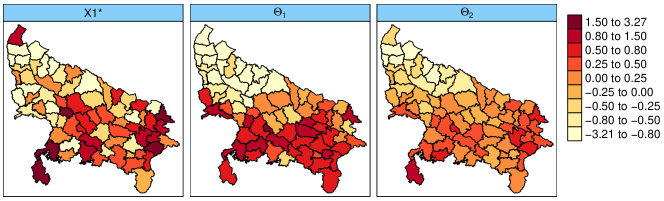
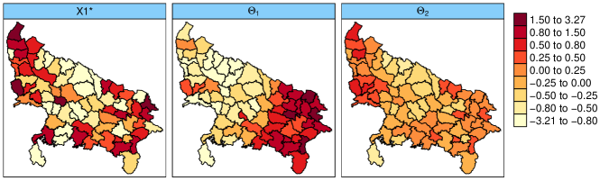
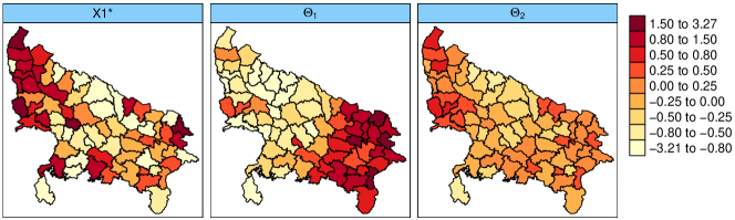
| ICAR | PCAR | BYM2 | ||||||||
| Model | Median | CI | Median | CI | Median | CI | ||||
| Scenario 3 | M-Spatial | 0.6203 | 0.3352 | 0.8260 | 0.6418 | 0.4166 | 0.8199 | 0.7990 | 0.5477 | 0.9377 |
| M-SpatPlus64 | 0.6126 | 0.3536 | 0.8014 | 0.6462 | 0.4428 | 0.8016 | 0.7140 | 0.4357 | 0.8897 | |
| M-SpatPlus59 | 0.5834 | 0.3198 | 0.7797 | 0.6232 | 0.4125 | 0.7864 | 0.6801 | 0.3979 | 0.8674 | |
| M-SpatPlus54 | 0.5828 | 0.3236 | 0.7758 | 0.6172 | 0.4091 | 0.7805 | 0.6834 | 0.3991 | 0.8716 | |
| M-SpatPlus49 | 0.6073 | 0.3579 | 0.7920 | 0.6325 | 0.4258 | 0.7932 | 0.7046 | 0.4330 | 0.8810 | |
| M-SpatPlus44 | 0.6092 | 0.3654 | 0.7900 | 0.6279 | 0.4240 | 0.7877 | 0.7168 | 0.4499 | 0.8896 | |
| M-SpatPlus39 | 0.5939 | 0.3435 | 0.7810 | 0.6166 | 0.4060 | 0.7816 | 0.7076 | 0.4324 | 0.8870 | |
| Scenario 4 | M-Spatial | 0.4241 | 0.1001 | 0.6840 | 0.2636 | -0.0474 | 0.5602 | 0.4675 | 0.1177 | 0.7309 |
| M-SpatPlus64 | 0.4637 | 0.1638 | 0.7025 | 0.3693 | 0.0808 | 0.6334 | 0.5192 | 0.2178 | 0.7557 | |
| M-SpatPlus59 | 0.5060 | 0.2373 | 0.7170 | 0.4268 | 0.1553 | 0.6666 | 0.5622 | 0.2943 | 0.7680 | |
| M-SpatPlus54 | 0.4995 | 0.2308 | 0.7115 | 0.4195 | 0.1455 | 0.6612 | 0.5566 | 0.2879 | 0.7644 | |
| M-SpatPlus49 | 0.5190 | 0.2562 | 0.7248 | 0.4416 | 0.1662 | 0.6824 | 0.5738 | 0.3085 | 0.7777 | |
| M-SpatPlus44 | 0.5437 | 0.2947 | 0.7387 | 0.4648 | 0.1944 | 0.6977 | 0.6016 | 0.3478 | 0.7931 | |
| M-SpatPlus39 | 0.5535 | 0.3082 | 0.7448 | 0.4730 | 0.2012 | 0.7052 | 0.6144 | 0.3685 | 0.8000 | |
| Scenario 5 | M-Spatial | 0.5283 | 0.2245 | 0.7629 | 0.3750 | 0.0832 | 0.6423 | 0.6028 | 0.2939 | 0.8212 |
| M-SpatPlus64 | 0.4963 | 0.2045 | 0.7218 | 0.4127 | 0.1107 | 0.6768 | 0.5293 | 0.2380 | 0.7546 | |
| M-SpatPlus59 | 0.5199 | 0.2571 | 0.7243 | 0.4543 | 0.1797 | 0.6892 | 0.5594 | 0.2950 | 0.7638 | |
| M-SpatPlus54 | 0.5011 | 0.2357 | 0.7091 | 0.4350 | 0.1562 | 0.6751 | 0.5404 | 0.2738 | 0.7488 | |
| M-SpatPlus49 | 0.5049 | 0.2409 | 0.7125 | 0.4391 | 0.1613 | 0.6772 | 0.5447 | 0.2798 | 0.7527 | |
| M-SpatPlus44 | 0.5287 | 0.2761 | 0.7275 | 0.4650 | 0.1943 | 0.6956 | 0.5704 | 0.3157 | 0.7660 | |
| M-SpatPlus39 | 0.5217 | 0.2701 | 0.7214 | 0.4528 | 0.1773 | 0.6895 | 0.5742 | 0.3167 | 0.7730 | |
| ICAR | PCAR | BYM2 | ||||||
| Model | True value | Mean | SD | Mean | SD | Mean | SD | |
| Scenario 3 | M-Spatial | 0.1500 | 0.2715 | 0.0807 | 0.2753 | 0.0813 | 0.2720 | 0.0822 |
| M-SpatPlus64 | 0.1948 | 0.0657 | 0.1921 | 0.0653 | 0.1925 | 0.0670 | ||
| M-SpatPlus59 | 0.1927 | 0.0626 | 0.1909 | 0.0624 | 0.1931 | 0.0641 | ||
| M-SpatPlus54 | 0.1758 | 0.0595 | 0.1745 | 0.0593 | 0.1764 | 0.0611 | ||
| M-SpatPlus49 | 0.1527 | 0.0576 | 0.1511 | 0.0575 | 0.1519 | 0.0595 | ||
| M-SpatPlus44 | 0.1389 | 0.0554 | 0.1379 | 0.0554 | 0.1386 | 0.0578 | ||
| M-SpatPlus39 | 0.1465 | 0.0538 | 0.1455 | 0.0539 | 0.1475 | 0.0563 | ||
| Scenario 4 | M-Spatial | 0.1500 | 0.3082 | 0.0726 | 0.3111 | 0.0751 | 0.3149 | 0.0747 |
| M-SpatPlus64 | 0.2722 | 0.0686 | 0.2725 | 0.0709 | 0.2743 | 0.0703 | ||
| M-SpatPlus59 | 0.2213 | 0.0648 | 0.2193 | 0.0672 | 0.2193 | 0.0661 | ||
| M-SpatPlus54 | 0.2205 | 0.0632 | 0.2190 | 0.0656 | 0.2194 | 0.0646 | ||
| M-SpatPlus49 | 0.2018 | 0.0619 | 0.2004 | 0.0642 | 0.2005 | 0.0634 | ||
| M-SpatPlus44 | 0.1758 | 0.0607 | 0.1743 | 0.0630 | 0.1743 | 0.0628 | ||
| M-SpatPlus39 | 0.1536 | 0.0568 | 0.1527 | 0.0592 | 0.1529 | 0.0596 | ||
| Scenario 5 | M-Spatial | 0.1500 | 0.2368 | 0.0776 | 0.2317 | 0.0799 | 0.2374 | 0.0792 |
| M-SpatPlus64 | 0.2096 | 0.0703 | 0.2104 | 0.0724 | 0.2111 | 0.0718 | ||
| M-SpatPlus59 | 0.1635 | 0.0660 | 0.1618 | 0.0682 | 0.1602 | 0.0674 | ||
| M-SpatPlus54 | 0.1661 | 0.0640 | 0.1648 | 0.0662 | 0.1639 | 0.0655 | ||
| M-SpatPlus49 | 0.1572 | 0.0624 | 0.1559 | 0.0646 | 0.1555 | 0.0641 | ||
| M-SpatPlus44 | 0.1312 | 0.0612 | 0.1300 | 0.0633 | 0.1288 | 0.0633 | ||
| M-SpatPlus39 | 0.1202 | 0.0571 | 0.1194 | 0.0593 | 0.1188 | 0.0599 | ||
| ICAR | PCAR | BYM2 | ||||||
| Model | True value | Mean | SD | Mean | SD | Mean | SD | |
| Scenario 3 | M-Spatial | 0.2000 | 0.3540 | 0.0423 | 0.3788 | 0.0446 | 0.3759 | 0.0442 |
| M-SpatPlus64 | 0.2602 | 0.0381 | 0.2633 | 0.0425 | 0.2630 | 0.0412 | ||
| M-SpatPlus59 | 0.2402 | 0.0375 | 0.2413 | 0.0415 | 0.2401 | 0.0405 | ||
| M-SpatPlus54 | 0.2132 | 0.0368 | 0.2144 | 0.0407 | 0.2111 | 0.0399 | ||
| M-SpatPlus49 | 0.1977 | 0.0357 | 0.1998 | 0.0394 | 0.1962 | 0.0389 | ||
| M-SpatPlus44 | 0.1780 | 0.0359 | 0.1793 | 0.0392 | 0.1773 | 0.0397 | ||
| M-SpatPlus39 | 0.1764 | 0.0350 | 0.1776 | 0.0384 | 0.1761 | 0.0389 | ||
| Scenario 4 | M-Spatial | 0.2000 | 0.3474 | 0.0384 | 0.3578 | 0.0398 | 0.3648 | 0.0399 |
| M-SpatPlus64 | 0.3157 | 0.0378 | 0.3177 | 0.0389 | 0.3259 | 0.0395 | ||
| M-SpatPlus59 | 0.2603 | 0.0391 | 0.2612 | 0.0399 | 0.2623 | 0.0409 | ||
| M-SpatPlus54 | 0.2479 | 0.0385 | 0.2486 | 0.0393 | 0.2491 | 0.0404 | ||
| M-SpatPlus49 | 0.2333 | 0.0380 | 0.2333 | 0.0387 | 0.2344 | 0.0399 | ||
| M-SpatPlus44 | 0.2049 | 0.0389 | 0.2051 | 0.0395 | 0.2066 | 0.0413 | ||
| M-SpatPlus39 | 0.1620 | 0.0380 | 0.1623 | 0.0386 | 0.1635 | 0.0409 | ||
| Scenario 5 | M-Spatial | 0.2000 | 0.3707 | 0.0392 | 0.3883 | 0.0404 | 0.3899 | 0.0405 |
| M-SpatPlus64 | 0.3251 | 0.0379 | 0.3257 | 0.0388 | 0.3327 | 0.0393 | ||
| M-SpatPlus59 | 0.2702 | 0.0394 | 0.2704 | 0.0402 | 0.2714 | 0.0411 | ||
| M-SpatPlus54 | 0.2542 | 0.0387 | 0.2545 | 0.0394 | 0.2548 | 0.0404 | ||
| M-SpatPlus49 | 0.2396 | 0.0382 | 0.2395 | 0.0389 | 0.2401 | 0.0400 | ||
| M-SpatPlus44 | 0.2140 | 0.0390 | 0.2139 | 0.0397 | 0.2150 | 0.0412 | ||
| M-SpatPlus39 | 0.1680 | 0.0384 | 0.1680 | 0.0390 | 0.1689 | 0.0411 | ||
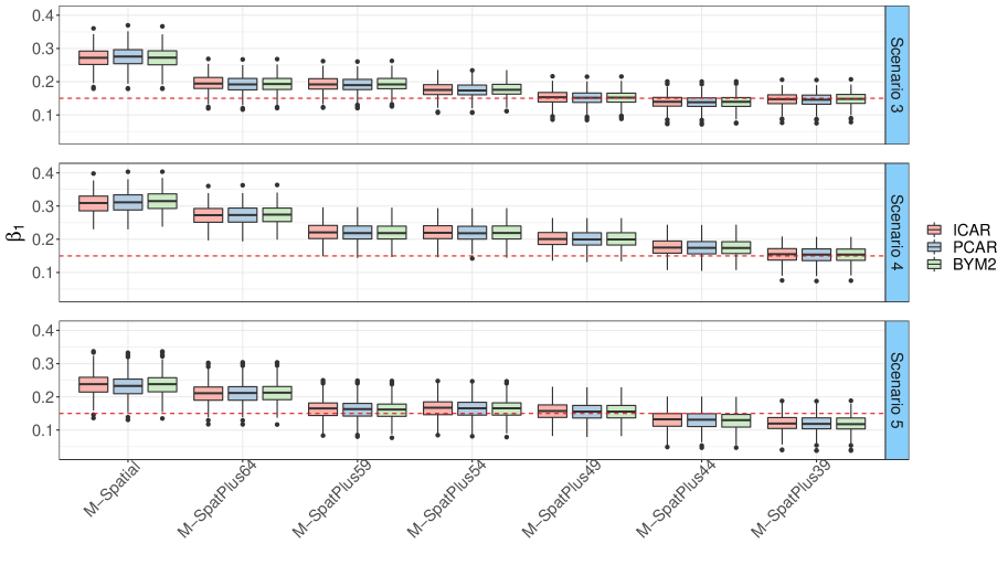
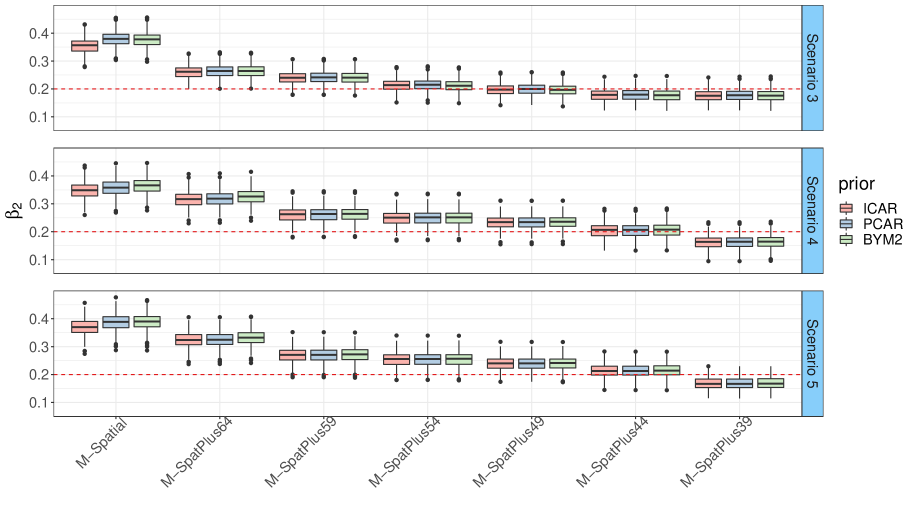
| ICAR | PCAR | BYM2 | |||||
| Model | |||||||
| Scenario 1 | M-Spatial | 0.0815 | 0.0338 | 0.0519 | 0.0290 | 0.0846 | 0.0338 |
| M-SpatPlus64 | 0.0612 | 0.0254 | 0.0404 | 0.0214 | 0.0630 | 0.0253 | |
| M-SpatPlus59 | 0.0585 | 0.0249 | 0.0393 | 0.0206 | 0.0605 | 0.0250 | |
| M-SpatPlus54 | 0.0580 | 0.0242 | 0.0390 | 0.0199 | 0.0599 | 0.0242 | |
| M-SpatPlus49 | 0.0563 | 0.0225 | 0.0378 | 0.0191 | 0.0584 | 0.0225 | |
| M-SpatPlus44 | 0.0547 | 0.0228 | 0.0555 | 0.0228 | 0.0574 | 0.0230 | |
| M-SpatPlus39 | 0.0517 | 0.0204 | 0.0526 | 0.0204 | 0.0549 | 0.0205 | |
| Scenario 2 | M-Spatial | 0.0685 | 0.0295 | 0.0712 | 0.0299 | 0.0708 | 0.0291 |
| M-SpatPlus64 | 0.0656 | 0.0283 | 0.0681 | 0.0286 | 0.0675 | 0.0280 | |
| M-SpatPlus59 | 0.0640 | 0.0275 | 0.0665 | 0.0278 | 0.0656 | 0.0272 | |
| M-SpatPlus54 | 0.0625 | 0.0268 | 0.0650 | 0.0271 | 0.0642 | 0.0265 | |
| M-SpatPlus49 | 0.0612 | 0.0252 | 0.0636 | 0.0255 | 0.0631 | 0.0249 | |
| M-SpatPlus44 | 0.0599 | 0.0266 | 0.0624 | 0.0268 | 0.0624 | 0.0267 | |
| M-SpatPlus39 | 0.0568 | 0.0239 | 0.0593 | 0.0241 | 0.0599 | 0.0239 | |
| Scenario 3 | M-Spatial | 0.0807 | 0.0301 | 0.0813 | 0.0307 | 0.0822 | 0.0302 |
| M-SpatPlus64 | 0.0657 | 0.0246 | 0.0653 | 0.0245 | 0.0670 | 0.0245 | |
| M-SpatPlus59 | 0.0626 | 0.0235 | 0.0624 | 0.0234 | 0.0641 | 0.0234 | |
| M-SpatPlus54 | 0.0595 | 0.0222 | 0.0593 | 0.0221 | 0.0611 | 0.0221 | |
| M-SpatPlus49 | 0.0576 | 0.0211 | 0.0575 | 0.0211 | 0.0595 | 0.0209 | |
| M-SpatPlus44 | 0.0554 | 0.0208 | 0.0554 | 0.0208 | 0.0578 | 0.0207 | |
| M-SpatPlus39 | 0.0538 | 0.0203 | 0.0539 | 0.0203 | 0.0563 | 0.0203 | |
| Scenario 4 | M-Spatial | 0.0726 | 0.0316 | 0.0751 | 0.0318 | 0.0747 | 0.0310 |
| M-SpatPlus64 | 0.0686 | 0.0300 | 0.0709 | 0.0302 | 0.0703 | 0.0296 | |
| M-SpatPlus59 | 0.0648 | 0.0277 | 0.0672 | 0.0280 | 0.0661 | 0.0275 | |
| M-SpatPlus54 | 0.0632 | 0.0269 | 0.0656 | 0.0273 | 0.0646 | 0.0268 | |
| M-SpatPlus49 | 0.0619 | 0.0256 | 0.0642 | 0.0259 | 0.0634 | 0.0255 | |
| M-SpatPlus44 | 0.0607 | 0.0265 | 0.0630 | 0.0268 | 0.0628 | 0.0266 | |
| M-SpatPlus39 | 0.0568 | 0.0235 | 0.0592 | 0.0238 | 0.0596 | 0.0235 | |
| Scenario 5 | M-Spatial | 0.0776 | 0.0342 | 0.0799 | 0.0344 | 0.0792 | 0.0334 |
| M-SpatPlus64 | 0.0703 | 0.0312 | 0.0724 | 0.0315 | 0.0718 | 0.0307 | |
| M-SpatPlus59 | 0.0660 | 0.0294 | 0.0682 | 0.0296 | 0.0674 | 0.0292 | |
| M-SpatPlus54 | 0.0640 | 0.0285 | 0.0662 | 0.0287 | 0.0655 | 0.0283 | |
| M-SpatPlus49 | 0.0624 | 0.0268 | 0.0646 | 0.0271 | 0.0641 | 0.0266 | |
| M-SpatPlus44 | 0.0612 | 0.0279 | 0.0633 | 0.0281 | 0.0633 | 0.0280 | |
| M-SpatPlus39 | 0.0571 | 0.0259 | 0.0593 | 0.0262 | 0.0599 | 0.0260 | |
| ICAR | PCAR | BYM2 | |||||
| Model | |||||||
| Scenario 1 | M-Spatial | 0.0476 | 0.0272 | 0.0519 | 0.0290 | 0.0501 | 0.0275 |
| M-SpatPlus64 | 0.0380 | 0.0210 | 0.0404 | 0.0214 | 0.0398 | 0.0211 | |
| M-SpatPlus59 | 0.0370 | 0.0203 | 0.0393 | 0.0206 | 0.0388 | 0.0203 | |
| M-SpatPlus54 | 0.0367 | 0.0196 | 0.0390 | 0.0199 | 0.0385 | 0.0197 | |
| M-SpatPlus49 | 0.0355 | 0.0189 | 0.0378 | 0.0191 | 0.0374 | 0.0189 | |
| M-SpatPlus44 | 0.0353 | 0.0199 | 0.0375 | 0.0201 | 0.0375 | 0.0201 | |
| M-SpatPlus39 | 0.0341 | 0.0184 | 0.0364 | 0.0186 | 0.0367 | 0.0186 | |
| Scenario 2 | M-Spatial | 0.0381 | 0.0285 | 0.0393 | 0.0286 | 0.0399 | 0.0279 |
| M-SpatPlus64 | 0.0371 | 0.0276 | 0.0382 | 0.0278 | 0.0392 | 0.0274 | |
| M-SpatPlus59 | 0.0380 | 0.0272 | 0.0389 | 0.0273 | 0.0401 | 0.0270 | |
| M-SpatPlus54 | 0.0374 | 0.0265 | 0.0383 | 0.0266 | 0.0395 | 0.0263 | |
| M-SpatPlus49 | 0.0368 | 0.0258 | 0.0376 | 0.0258 | 0.0389 | 0.0256 | |
| M-SpatPlus44 | 0.0378 | 0.0261 | 0.0384 | 0.0261 | 0.0404 | 0.0261 | |
| M-SpatPlus39 | 0.0373 | 0.0252 | 0.0379 | 0.0252 | 0.0404 | 0.0254 | |
| Scenario 3 | M-Spatial | 0.0423 | 0.0284 | 0.0446 | 0.0281 | 0.0442 | 0.0276 |
| M-SpatPlus64 | 0.0381 | 0.0242 | 0.0425 | 0.0250 | 0.0412 | 0.0244 | |
| M-SpatPlus59 | 0.0375 | 0.0235 | 0.0415 | 0.0241 | 0.0405 | 0.0237 | |
| M-SpatPlus54 | 0.0368 | 0.0222 | 0.0407 | 0.0228 | 0.0399 | 0.0224 | |
| M-SpatPlus49 | 0.0357 | 0.0210 | 0.0394 | 0.0216 | 0.0389 | 0.0212 | |
| M-SpatPlus44 | 0.0359 | 0.0220 | 0.0392 | 0.0223 | 0.0397 | 0.0224 | |
| M-SpatPlus39 | 0.0350 | 0.0218 | 0.0384 | 0.0221 | 0.0389 | 0.0222 | |
| Scenario 4 | M-Spatial | 0.0384 | 0.0290 | 0.0398 | 0.0295 | 0.0399 | 0.0280 |
| M-SpatPlus64 | 0.0378 | 0.0279 | 0.0389 | 0.0279 | 0.0395 | 0.0273 | |
| M-SpatPlus59 | 0.0391 | 0.0267 | 0.0399 | 0.0268 | 0.0409 | 0.0265 | |
| M-SpatPlus54 | 0.0385 | 0.0263 | 0.0393 | 0.0263 | 0.0404 | 0.0261 | |
| M-SpatPlus49 | 0.0380 | 0.0254 | 0.0387 | 0.0254 | 0.0399 | 0.0252 | |
| M-SpatPlus44 | 0.0389 | 0.0262 | 0.0395 | 0.0262 | 0.0413 | 0.0262 | |
| M-SpatPlus39 | 0.0380 | 0.0243 | 0.0386 | 0.0243 | 0.0409 | 0.0244 | |
| Scenario 5 | M-Spatial | 0.0392 | 0.0289 | 0.0404 | 0.0297 | 0.0405 | 0.0284 |
| M-SpatPlus64 | 0.0379 | 0.0271 | 0.0388 | 0.0272 | 0.0393 | 0.0271 | |
| M-SpatPlus59 | 0.0394 | 0.0262 | 0.0402 | 0.0263 | 0.0411 | 0.0263 | |
| M-SpatPlus54 | 0.0387 | 0.0253 | 0.0394 | 0.0253 | 0.0404 | 0.0254 | |
| M-SpatPlus49 | 0.0382 | 0.0240 | 0.0389 | 0.0240 | 0.0400 | 0.0240 | |
| M-SpatPlus44 | 0.0390 | 0.0241 | 0.0397 | 0.0241 | 0.0412 | 0.0243 | |
| M-SpatPlus39 | 0.0384 | 0.0222 | 0.0390 | 0.0223 | 0.0411 | 0.0224 | |
| ICAR | PCAR | BYM2 | ICAR | PCAR | BYM2 | ||
| Scenario 3 | M-Spatial | 88.3333 | 85.3333 | 89.3333 | 1.3333 | 0.0000 | 0.0000 |
| M-SpatPlus64 | 100.0000 | 100.0000 | 100.0000 | 73.6667 | 80.6667 | 78.0000 | |
| M-SpatPlus59 | 100.0000 | 100.0000 | 100.0000 | 92.6667 | 95.6667 | 95.6667 | |
| M-SpatPlus54 | 100.0000 | 100.0000 | 100.0000 | 99.0000 | 99.6667 | 99.6667 | |
| M-SpatPlus49 | 100.0000 | 100.0000 | 100.0000 | 100.0000 | 100.0000 | 100.0000 | |
| M-SpatPlus44 | 100.0000 | 100.0000 | 100.0000 | 98.6667 | 99.6667 | 99.6667 | |
| M-SpatPlus39 | 100.0000 | 100.0000 | 100.0000 | 98.0000 | 99.3333 | 99.0000 | |
| Scenario 4 | M-Spatial | 31.6667 | 35.0000 | 28.3333 | 0.6667 | 0.6667 | 0.3333 |
| M-SpatPlus64 | 64.3333 | 68.3333 | 66.0000 | 8.0000 | 8.0000 | 4.0000 | |
| M-SpatPlus59 | 98.0000 | 99.0000 | 99.0000 | 70.3333 | 72.0000 | 71.0000 | |
| M-SpatPlus54 | 97.6667 | 99.0000 | 98.0000 | 88.3333 | 89.0000 | 90.6667 | |
| M-SpatPlus49 | 100.0000 | 100.0000 | 100.0000 | 94.6667 | 94.6667 | 95.6667 | |
| M-SpatPlus44 | 100.0000 | 100.0000 | 100.0000 | 99.3333 | 99.3333 | 99.3333 | |
| M-SpatPlus39 | 100.0000 | 100.0000 | 100.0000 | 92.6667 | 94.0000 | 95.3333 | |
| Scenario 5 | M-Spatial | 96.6667 | 98.6667 | 96.6667 | 0.3333 | 0.0000 | 0.0000 |
| M-SpatPlus64 | 99.3333 | 99.3333 | 99.3333 | 2.3333 | 2.6667 | 2.0000 | |
| M-SpatPlus59 | 100.0000 | 100.0000 | 100.0000 | 59.0000 | 61.0000 | 62.6667 | |
| M-SpatPlus54 | 100.0000 | 100.0000 | 100.0000 | 82.0000 | 83.6667 | 85.6667 | |
| M-SpatPlus49 | 100.0000 | 100.0000 | 100.0000 | 93.3333 | 94.0000 | 94.6667 | |
| M-Spatplus44 | 100.0000 | 100.0000 | 100.0000 | 99.3333 | 99.3333 | 99.3333 | |
| M-SpatPlus39 | 100.0000 | 100.0000 | 100.0000 | 96.6667 | 97.3333 | 98.3333 | |
| ICAR | PCAR | BYM2 | |||||
| Model | DIC | WAIC | DIC | WAIC | DIC | WAIC | |
| Scenario 3 | M-Spatial | 967.9454 | 954.5795 | 967.5495 | 952.1199 | 967.9909 | 951.7634 |
| M-SpatPlus64 | 969.1749 | 951.7115 | 970.9422 | 951.6440 | 970.9431 | 950.8905 | |
| M-SpatPlus59 | 970.2056 | 951.4510 | 972.0560 | 951.7777 | 972.2680 | 951.2902 | |
| M-SpatPlus54 | 972.2309 | 953.1453 | 973.6655 | 952.8703 | 974.4395 | 953.3604 | |
| M-SpatPlus49 | 973.2094 | 954.5434 | 974.3598 | 953.7926 | 975.3738 | 954.5668 | |
| M-SpatPlus44 | 974.3461 | 955.1660 | 975.2471 | 954.0045 | 976.5248 | 955.1149 | |
| M-SpatPlus39 | 974.7621 | 955.7078 | 975.6728 | 954.5366 | 976.9174 | 955.6734 | |
| Scenario 4 | M-Spatial | 966.8835 | 950.9785 | 967.8758 | 948.4934 | 967.5878 | 947.7641 |
| M-SpatPlus64 | 967.1693 | 949.2779 | 968.0115 | 946.6388 | 968.0098 | 946.4287 | |
| M-SpatPlus59 | 969.9224 | 948.3949 | 970.8501 | 946.1590 | 971.2409 | 947.0300 | |
| M-SpatPlus54 | 970.9355 | 949.3026 | 971.8493 | 947.1336 | 972.3405 | 948.2459 | |
| M-SpatPlus49 | 972.1451 | 950.7576 | 973.0600 | 948.5624 | 973.5596 | 949.7205 | |
| M-SpatPlus44 | 974.2859 | 952.6960 | 975.0717 | 950.2682 | 975.6985 | 951.5074 | |
| M-SpatPlus39 | 978.3585 | 957.7842 | 979.0163 | 955.1304 | 979.6206 | 956.2045 | |
| Scenario 5 | M-Spatial | 965.3720 | 950.3049 | 966.0718 | 947.7260 | 965.6266 | 946.7197 |
| M-SpatPlus64 | 965.5671 | 947.2383 | 966.5097 | 945.1004 | 966.4342 | 944.4985 | |
| M-SpatPlus59 | 968.6013 | 946.5191 | 969.6242 | 944.7155 | 969.9139 | 945.2128 | |
| M-SpatPlus54 | 969.9959 | 947.6624 | 971.0162 | 945.9452 | 971.4843 | 946.7808 | |
| M-SpatPlus49 | 971.3763 | 949.1848 | 972.3350 | 947.4099 | 972.8820 | 948.4109 | |
| M-SpatPlus44 | 973.5362 | 951.3029 | 974.4013 | 949.3644 | 975.0159 | 950.4543 | |
| M-SpatPlus39 | 978.1803 | 956.8477 | 978.9062 | 954.5679 | 979.5386 | 955.6113 | |
| ICAR | PCAR | BYM2 | |||||
| Model | MARB | MRRMSE | MARB | MRRMSE | MARB | MRRMSE | |
| Scenario 1 | M-Spatial | 0.0675 | 0.1550 | 0.0649 | 0.1567 | 0.0639 | 0.1557 |
| M-SpatPlus64 | 0.0652 | 0.1567 | 0.0632 | 0.1585 | 0.0626 | 0.1579 | |
| M-SpatPlus59 | 0.0660 | 0.1579 | 0.0643 | 0.1597 | 0.0642 | 0.1592 | |
| M-SpatPlus54 | 0.0657 | 0.1583 | 0.0638 | 0.1601 | 0.0639 | 0.1598 | |
| M-SpatPlus49 | 0.0694 | 0.1608 | 0.0671 | 0.1623 | 0.0676 | 0.1622 | |
| M-SpatPlus44 | 0.0695 | 0.1612 | 0.0671 | 0.1626 | 0.0677 | 0.1626 | |
| M-SpatPlus39 | 0.0737 | 0.1655 | 0.0705 | 0.1666 | 0.0715 | 0.1669 | |
| Scenario 2 | M-Spatial | 0.0634 | 0.1580 | 0.0597 | 0.1597 | 0.0602 | 0.1594 |
| M-SpatPlus64 | 0.0623 | 0.1585 | 0.0584 | 0.1601 | 0.0589 | 0.1598 | |
| M-SpatPlus59 | 0.0608 | 0.1606 | 0.0571 | 0.1621 | 0.0583 | 0.1621 | |
| M-SpatPlus54 | 0.0616 | 0.1615 | 0.0580 | 0.1630 | 0.0593 | 0.1630 | |
| M-SpatPlus49 | 0.0622 | 0.1632 | 0.0593 | 0.1646 | 0.0601 | 0.1647 | |
| M-SpatPlus44 | 0.0616 | 0.1649 | 0.0588 | 0.1663 | 0.0595 | 0.1664 | |
| M-SpatPlus39 | 0.0685 | 0.1705 | 0.0651 | 0.1718 | 0.0657 | 0.1718 | |
| Scenario 3 | M-Spatial | 0.0668 | 0.1545 | 0.0647 | 0.1555 | 0.0650 | 0.1555 |
| M-SpatPlus64 | 0.0625 | 0.1571 | 0.0614 | 0.1598 | 0.0608 | 0.1592 | |
| M-SpatPlus59 | 0.0618 | 0.1584 | 0.0617 | 0.1612 | 0.0609 | 0.1608 | |
| M-SpatPlus54 | 0.0633 | 0.1612 | 0.0624 | 0.1634 | 0.0627 | 0.1637 | |
| M-SpatPlus49 | 0.0669 | 0.1641 | 0.0650 | 0.1657 | 0.0659 | 0.1665 | |
| M-SpatPlus44 | 0.0652 | 0.1648 | 0.0637 | 0.1663 | 0.0644 | 0.1673 | |
| M-SpatPlus39 | 0.0674 | 0.1661 | 0.0654 | 0.1674 | 0.0665 | 0.1684 | |
| Scenario 4 | M-Spatial | 0.0621 | 0.1540 | 0.0588 | 0.1557 | 0.0596 | 0.1554 |
| M-SpatPlus64 | 0.0600 | 0.1552 | 0.0564 | 0.1569 | 0.0572 | 0.1566 | |
| M-SpatPlus59 | 0.0586 | 0.1596 | 0.0550 | 0.1612 | 0.0569 | 0.1612 | |
| M-SpatPlus54 | 0.0595 | 0.1608 | 0.0559 | 0.1623 | 0.0578 | 0.1625 | |
| M-SpatPlus49 | 0.0608 | 0.1627 | 0.0578 | 0.1642 | 0.0594 | 0.1643 | |
| M-SpatPlus44 | 0.0602 | 0.1643 | 0.0570 | 0.1657 | 0.0584 | 0.1659 | |
| M-SpatPlus39 | 0.0691 | 0.1706 | 0.0654 | 0.1718 | 0.0665 | 0.1719 | |
| Scenario 5 | M-Spatial | 0.0594 | 0.1511 | 0.0571 | 0.1528 | 0.0574 | 0.1524 |
| M-SpatPlus64 | 0.0559 | 0.1527 | 0.0534 | 0.1545 | 0.0536 | 0.1543 | |
| M-SpatPlus59 | 0.0547 | 0.1573 | 0.0519 | 0.1589 | 0.0532 | 0.1590 | |
| M-SpatPlus54 | 0.0559 | 0.1590 | 0.0533 | 0.1606 | 0.0548 | 0.1608 | |
| M-SpatPlus49 | 0.0575 | 0.1606 | 0.0550 | 0.1622 | 0.0565 | 0.1625 | |
| M-SpatPlus44 | 0.0564 | 0.1625 | 0.0539 | 0.1640 | 0.0554 | 0.1643 | |
| M-SpatPlus39 | 0.0642 | 0.1688 | 0.0611 | 0.1701 | 0.0624 | 0.1703 | |
| Model | ICAR | PCAR | BYM2 | ICAR | PCAR | BYM2 | |
| Scenario 1 | M-Spatial | 0.3208 | 0.3293 | 0.3328 | 0.1871 | 0.2039 | 0.1972 |
| M-SpatPlus64 | 0.2407 | 0.2435 | 0.2478 | 0.1495 | 0.1587 | 0.1565 | |
| M-SpatPlus59 | 0.2304 | 0.2331 | 0.2382 | 0.1455 | 0.1546 | 0.1527 | |
| M-SpatPlus54 | 0.2280 | 0.2309 | 0.2358 | 0.1443 | 0.1534 | 0.1516 | |
| M-SpatPlus49 | 0.2215 | 0.2245 | 0.2298 | 0.1395 | 0.1485 | 0.1469 | |
| M-SpatPlus44 | 0.2154 | 0.2184 | 0.2259 | 0.1389 | 0.1474 | 0.1476 | |
| M-SpatPlus39 | 0.2036 | 0.2067 | 0.2161 | 0.1341 | 0.1429 | 0.1442 | |
| Scenario 2 | M-Spatial | 0.2694 | 0.2800 | 0.2785 | 0.1499 | 0.1543 | 0.1569 |
| M-SpatPlus64 | 0.2579 | 0.2678 | 0.2655 | 0.1460 | 0.1502 | 0.1542 | |
| M-SpatPlus59 | 0.2515 | 0.2615 | 0.2582 | 0.1495 | 0.1530 | 0.1575 | |
| M-SpatPlus54 | 0.2457 | 0.2555 | 0.2524 | 0.1472 | 0.1505 | 0.1552 | |
| M-SpatPlus49 | 0.2408 | 0.2503 | 0.2481 | 0.1448 | 0.1478 | 0.1531 | |
| M-SpatPlus44 | 0.2355 | 0.2453 | 0.2455 | 0.1485 | 0.1509 | 0.1588 | |
| M-SpatPlus39 | 0.2232 | 0.2331 | 0.2358 | 0.1467 | 0.1488 | 0.1588 | |
| Scenario 3 | M-Spatial | 0.3175 | 0.3197 | 0.3234 | 0.1664 | 0.1753 | 0.1736 |
| M-SpatPlus64 | 0.2584 | 0.2567 | 0.2635 | 0.1499 | 0.1671 | 0.1619 | |
| M-SpatPlus59 | 0.2464 | 0.2452 | 0.2522 | 0.1474 | 0.1632 | 0.1591 | |
| M-SpatPlus54 | 0.2341 | 0.2330 | 0.2404 | 0.1445 | 0.1598 | 0.1570 | |
| M-SpatPlus49 | 0.2266 | 0.2261 | 0.2340 | 0.1402 | 0.1547 | 0.1531 | |
| M-SpatPlus44 | 0.2179 | 0.2178 | 0.2274 | 0.1410 | 0.1540 | 0.1560 | |
| M-SpatPlus39 | 0.2118 | 0.2118 | 0.2215 | 0.1377 | 0.1509 | 0.1532 | |
| Scenario 4 | M-Spatial | 0.2855 | 0.2953 | 0.2940 | 0.1509 | 0.1566 | 0.1570 |
| M-SpatPlus64 | 0.2699 | 0.2788 | 0.2764 | 0.1486 | 0.1530 | 0.1554 | |
| M-SpatPlus59 | 0.2547 | 0.2641 | 0.2601 | 0.1535 | 0.1568 | 0.1608 | |
| M-SpatPlus54 | 0.2486 | 0.2579 | 0.2541 | 0.1514 | 0.1546 | 0.1589 | |
| M-SpatPlus49 | 0.2434 | 0.2525 | 0.2494 | 0.1492 | 0.1522 | 0.1570 | |
| M-SpatPlus44 | 0.2385 | 0.2477 | 0.2471 | 0.1529 | 0.1554 | 0.1625 | |
| M-SpatPlus39 | 0.2234 | 0.2327 | 0.2346 | 0.1494 | 0.1517 | 0.1610 | |
| Scenario 5 | M-Spatial | 0.3051 | 0.3141 | 0.3113 | 0.1540 | 0.1585 | 0.1592 |
| M-SpatPlus64 | 0.2764 | 0.2849 | 0.2825 | 0.1488 | 0.1526 | 0.1544 | |
| M-SpatPlus59 | 0.2595 | 0.2683 | 0.2650 | 0.1548 | 0.1579 | 0.1614 | |
| M-SpatPlus54 | 0.2515 | 0.2602 | 0.2576 | 0.1520 | 0.1550 | 0.1589 | |
| M-SpatPlus49 | 0.2456 | 0.2539 | 0.2521 | 0.1501 | 0.1531 | 0.1572 | |
| M-SpatPlus44 | 0.2405 | 0.2489 | 0.2490 | 0.1534 | 0.1560 | 0.1621 | |
| M-SpatPlus39 | 0.2246 | 0.2332 | 0.2356 | 0.1507 | 0.1534 | 0.1618 | |
| ICAR | PCAR | BYM2 | |||||
| Model | MARB | MRRMSE | MARB | MRRMSE | MARB | MRRMSE | |
| Scenario 1 | M-Spatial | 0.8006 | 0.8317 | 0.8439 | 0.8738 | 0.8399 | 0.8696 |
| M-SpatPlus64 | 0.2523 | 0.3038 | 0.2473 | 0.2997 | 0.2635 | 0.3130 | |
| M-SpatPlus59 | 0.2762 | 0.3223 | 0.2766 | 0.3227 | 0.3076 | 0.3500 | |
| M-SpatPlus54 | 0.1391 | 0.2129 | 0.1365 | 0.2114 | 0.1541 | 0.2233 | |
| M-SpatPlus49 | 0.0534 | 0.1595 | 0.0527 | 0.1594 | 0.0663 | 0.1642 | |
| M-SpatPlus44 | 0.0632 | 0.1645 | 0.0618 | 0.1642 | 0.0499 | 0.1611 | |
| M-SpatPlus39 | 0.1601 | 0.2101 | 0.1598 | 0.2100 | 0.1407 | 0.1961 | |
| Scenario 2 | M-Spatial | 0.7923 | 0.8164 | 0.8174 | 0.8414 | 0.8222 | 0.8448 |
| M-SpatPlus64 | 0.6038 | 0.6326 | 0.5998 | 0.6295 | 0.6044 | 0.6326 | |
| M-SpatPlus59 | 0.4398 | 0.4764 | 0.4267 | 0.4652 | 0.4265 | 0.4635 | |
| M-SpatPlus54 | 0.4486 | 0.4828 | 0.4380 | 0.4738 | 0.4424 | 0.4765 | |
| M-SpatPlus49 | 0.3310 | 0.3712 | 0.3216 | 0.3637 | 0.3233 | 0.3635 | |
| M-SpatPlus44 | 0.1332 | 0.2217 | 0.1235 | 0.2174 | 0.1222 | 0.2156 | |
| M-SpatPlus39 | 0.0304 | 0.1623 | 0.0368 | 0.1651 | 0.0395 | 0.1639 | |
| Scenario 3 | M-Spatial | 0.8103 | 0.8347 | 0.8355 | 0.8602 | 0.8133 | 0.8378 |
| M-SpatPlus64 | 0.2987 | 0.3408 | 0.2809 | 0.3250 | 0.2833 | 0.3270 | |
| M-SpatPlus59 | 0.2849 | 0.3251 | 0.2730 | 0.3144 | 0.2871 | 0.3267 | |
| M-SpatPlus54 | 0.1723 | 0.2271 | 0.1634 | 0.2199 | 0.1762 | 0.2295 | |
| M-SpatPlus49 | 0.0178 | 0.1415 | 0.0074 | 0.1406 | 0.0129 | 0.1400 | |
| M-SpatPlus44 | 0.0739 | 0.1570 | 0.0810 | 0.1604 | 0.0761 | 0.1578 | |
| M-SpatPlus39 | 0.0235 | 0.1376 | 0.0299 | 0.1387 | 0.0164 | 0.1360 | |
| Scenario 4 | M-Spatial | 1.0548 | 1.0756 | 1.0739 | 1.0947 | 1.0995 | 1.1188 |
| M-SpatPlus64 | 0.8148 | 0.8390 | 0.8169 | 0.8414 | 0.8285 | 0.8518 | |
| M-SpatPlus59 | 0.4753 | 0.5099 | 0.4623 | 0.4986 | 0.4622 | 0.4973 | |
| M-SpatPlus54 | 0.4700 | 0.5032 | 0.4598 | 0.4944 | 0.4627 | 0.4960 | |
| M-SpatPlus49 | 0.3457 | 0.3855 | 0.3359 | 0.3778 | 0.3368 | 0.3774 | |
| M-SpatPlus44 | 0.1719 | 0.2464 | 0.1623 | 0.2411 | 0.1619 | 0.2401 | |
| M-SpatPlus39 | 0.0240 | 0.1585 | 0.0178 | 0.1596 | 0.0193 | 0.1579 | |
| Scenario 5 | M-Spatial | 0.5787 | 0.6219 | 0.5447 | 0.5910 | 0.5826 | 0.6238 |
| M-SpatPlus64 | 0.3976 | 0.4488 | 0.4029 | 0.4542 | 0.4070 | 0.4557 | |
| M-SpatPlus59 | 0.0902 | 0.2156 | 0.0787 | 0.2125 | 0.0678 | 0.2060 | |
| M-SpatPlus54 | 0.1071 | 0.2178 | 0.0984 | 0.2151 | 0.0926 | 0.2102 | |
| M-SpatPlus49 | 0.0482 | 0.1852 | 0.0392 | 0.1846 | 0.0369 | 0.1814 | |
| M-SpatPlus44 | 0.1255 | 0.2244 | 0.1332 | 0.2299 | 0.1413 | 0.2339 | |
| M-SpatPlus39 | 0.1989 | 0.2636 | 0.2041 | 0.2685 | 0.2077 | 0.2704 | |
| ICAR | PCAR | BYM2 | |||||
| Model | MARB | MRRMSE | MARB | MRRMSE | MARB | MRRMSE | |
| Scenario 1 | M-Spatial | 0.5088 | 0.5267 | 0.6421 | 0.6583 | 0.5893 | 0.6051 |
| M-SpatPlus64 | 0.0274 | 0.1087 | 0.0255 | 0.1098 | 0.0345 | 0.1109 | |
| M-SpatPlus59 | 0.0309 | 0.1061 | 0.0327 | 0.1081 | 0.0263 | 0.1050 | |
| M-SpatPlus54 | 0.0854 | 0.1301 | 0.0856 | 0.1314 | 0.0850 | 0.1300 | |
| M-SpatPlus49 | 0.1297 | 0.1604 | 0.1303 | 0.1616 | 0.1277 | 0.1587 | |
| M-SpatPlus44 | 0.1976 | 0.2213 | 0.2003 | 0.2241 | 0.1936 | 0.2181 | |
| M-SpatPlus39 | 0.3479 | 0.3599 | 0.3492 | 0.3614 | 0.3440 | 0.3564 | |
| Scenario 2 | M-Spatial | 0.4378 | 0.4603 | 0.4570 | 0.4789 | 0.4984 | 0.5175 |
| M-SpatPlus64 | 0.3371 | 0.3643 | 0.3471 | 0.3738 | 0.3855 | 0.4091 | |
| M-SpatPlus59 | 0.1968 | 0.2392 | 0.2017 | 0.2436 | 0.2116 | 0.2509 | |
| M-SpatPlus54 | 0.1568 | 0.2053 | 0.1616 | 0.2092 | 0.1683 | 0.2134 | |
| M-SpatPlus49 | 0.0945 | 0.1599 | 0.0949 | 0.1601 | 0.1065 | 0.1666 | |
| M-SpatPlus44 | 0.0619 | 0.1445 | 0.0601 | 0.1436 | 0.0474 | 0.1391 | |
| M-SpatPlus39 | 0.2732 | 0.3009 | 0.2709 | 0.2988 | 0.2641 | 0.2931 | |
| Scenario 3 | M-Spatial | 0.7698 | 0.7827 | 0.8939 | 0.9049 | 0.8795 | 0.8902 |
| M-SpatPlus64 | 0.3011 | 0.3245 | 0.3167 | 0.3406 | 0.3150 | 0.3377 | |
| M-SpatPlus59 | 0.2010 | 0.2327 | 0.2063 | 0.2390 | 0.2004 | 0.2329 | |
| M-SpatPlus54 | 0.0659 | 0.1289 | 0.0721 | 0.1349 | 0.0556 | 0.1250 | |
| M-SpatPlus49 | 0.0115 | 0.1057 | 0.0009 | 0.1080 | 0.0188 | 0.1079 | |
| M-SpatPlus44 | 0.1098 | 0.1553 | 0.1034 | 0.1522 | 0.1133 | 0.1592 | |
| M-SpatPlus39 | 0.1181 | 0.1606 | 0.1122 | 0.1574 | 0.1193 | 0.1630 | |
| Scenario 4 | M-Spatial | 0.7372 | 0.7513 | 0.7891 | 0.8029 | 0.8242 | 0.8360 |
| M-SpatPlus64 | 0.5784 | 0.5950 | 0.5887 | 0.6051 | 0.6296 | 0.6442 | |
| M-SpatPlus59 | 0.3016 | 0.3298 | 0.3060 | 0.3340 | 0.3115 | 0.3385 | |
| M-SpatPlus54 | 0.2395 | 0.2732 | 0.2430 | 0.2763 | 0.2454 | 0.2779 | |
| M-SpatPlus49 | 0.1667 | 0.2094 | 0.1664 | 0.2093 | 0.1722 | 0.2133 | |
| M-SpatPlus44 | 0.0244 | 0.1333 | 0.0257 | 0.1335 | 0.0329 | 0.1348 | |
| M-SpatPlus39 | 0.1900 | 0.2256 | 0.1884 | 0.2242 | 0.1827 | 0.2198 | |
| Scenario 5 | M-Spatial | 0.8536 | 0.8657 | 0.9415 | 0.9531 | 0.9496 | 0.9602 |
| M-SpatPlus64 | 0.6253 | 0.6399 | 0.6285 | 0.6431 | 0.6637 | 0.6774 | |
| M-SpatPlus59 | 0.3510 | 0.3747 | 0.3518 | 0.3756 | 0.3568 | 0.3804 | |
| M-SpatPlus54 | 0.2712 | 0.2992 | 0.2725 | 0.3005 | 0.2739 | 0.3019 | |
| M-SpatPlus49 | 0.1982 | 0.2316 | 0.1973 | 0.2309 | 0.2004 | 0.2336 | |
| M-SpatPlus44 | 0.0699 | 0.1394 | 0.0696 | 0.1393 | 0.0749 | 0.1426 | |
| M-SpatPlus39 | 0.1601 | 0.1950 | 0.1600 | 0.1949 | 0.1555 | 0.1917 | |