Efficient Last-Iterate Convergence in Solving Games

Abstract

No-regret algorithms are popular for learning Nash equilibrium (NE) in two-player zero-sum normal-form games (NFGs) and extensive-form games (EFGs). However, most of them only have average-iterate convergence, which implies they must average strategies. Averaging strategies increases computational and memory overhead. Importantly, it may also cause additional representation errors when function approximation is used. Therefore, many recent works consider the last-iterate convergence no-regret algorithms since they do not require such averaging. Among them, the two most famous algorithms are Optimistic Gradient Descent Ascent (OGDA) and Optimistic Multiplicative Weight Update (OMWU). However, OGDA has high per-iteration complexity. OMWU exhibits a lower per-iteration complexity but poorer empirical performance, and its convergence holds only when NE is unique. Recent works propose a Reward Transformation (RT) framework for MWU, which removes the uniqueness condition and achieves competitive performance with OMWU. Unfortunately, the algorithms built by this framework perform worse than OGDA under the same number of iterations, and their convergence guarantee is based on the continuous-time feedback assumption, which does not hold in most scenarios. To address these issues, we provide a closer analysis of the RT framework, which holds for both continuous and discrete-time feedback. We demonstrate that the essence of the RT framework is to transform the problem of learning NE in the original game into a series of strongly convex-concave optimization problems (SCCPs), and the sequence of the saddle points of these SCCPs converges to NE of the original game. We show that the bottleneck of the algorithms built by the RT framework is the speed of solving SCCPs. To improve the RT framework’s empirical performance, we design a novel transformation method to enable the SCCPs can be solved by Regret Matching+ (RM+), a no-regret algorithm with better empirical performance than MWU, resulting in Reward Transformation RM+ (RTRM+). RTRM+ enjoys last-iterate convergence under the discrete-time feedback setting. Using the counterfactual regret decomposition framework, we propose Reward Transformation CFR+ (RTCFR+) to extend RTRM+ to EFGs. Experimental results on NFGs and EFGs show that our algorithms significantly outperform existing last-iterate convergence algorithms and RM+ (CFR+).

1 Introduction

Learning Nash equilibrium (NE) in two-player zero-sum games involves finding the saddle points of convex-concave optimization problems, which is critical in modern machine learning and decision-making paradigms, such as generative adversarial networks (Goodfellow et al., 2014), game theory (Osborne et al., 2004), and multi-agent reinforcement learning (Busoniu et al., 2008). No-regret algorithms, such as Gradient Descent Ascent (GDA) and Multiplicative Weight Updates (MWU), are the most widely used algorithms to find the saddle points. However, these algorithms usually only exhibit average-iterate convergence and will diverge or cycle even in two-player zero-sum normal-formal games (NFGs) (Bailey and Piliouras, 2018; Mertikopoulos et al., 2018; Pérolat et al., 2021). Therefore, to learn NE, these algorithms have to average strategies, which not only increases computational and memory overhead but also may cause additional representation errors when function approximation is used. Precisely, if the strategies are parameterized by approximation functions, a new approximation function has to be trained to represent the average strategy. Such training will incur additional representation errors. Therefore, algorithms whose sequence of evolving strategy profiles converges to NE, also called last-iterate convergence, are more desirable since they do not require such an averaging operation.

Recent research has demonstrated that Optimistic GDA (OGDA) and Optimistic MWU (OMWU) exhibit last-iterate convergence in two-player zero-sum NFGs (Wei et al., 2021) and extensive-form games (EFGs) (Lee et al., 2021). However, OGDA has high per-iteration complexity due to four costly projection operations at each iteration. OMWU exhibits a lower per-iteration complexity but poorer experimental performance and its convergence is based on the unique NE assumption. To remove the uniqueness condition, recent works propose a Reward Transformation (RT) framework for MWU (Bauer et al., 2019; Pérolat et al., 2021, 2022; Abe et al., 2022a, b). These algorithms apply an additional RT term to the feedback of MWU and achieve lower per-iteration computational overhead and competitive performance with OMWU. However, they perform worse than OGDA under the same number of iterations. Furthermore, their convergence guarantee is based on the continuous-time feedback assumption that does not hold in most scenarios..

Previous attempts to enhance the empirical performance of the RT framework focused on designing various RT terms. However, our analysis of the RT framework, which constitutes our first contribution, reveals that MWU, rather than the RT terms, may be responsible for the undesired performance of the RT framework. Specifically, we demonstrate that the RT framework’s essence is transforming the original convex-concave optimization problem into a series of strongly convex-concave optimization problems (SCCPs), with the sequence of saddle points of these SCCPs converging to the original problem’s saddle points. We show that the RT framework’s bottleneck is the speed of solving the SCCPs. In other words, despite the RT framework being designed for MWU, the poor empirical performance of MWU in solving SCCPs seriously compromises the RT framework’s empirical performance. More importantly, our analysis holds for both continuous and discrete-time feedback.

To improve the empirical performance of the RT framework, a straightforward approach is to use algorithms with better empirical performance than MWU to solve the SCCPs, such as regret matching+ (RM+) (Bowling et al., 2015; Farina et al., 2021a). However, this approach may not be practical since these algorithms will yield strategies on the boundary, while the domain of the transformed SCCPs used in previous studies of the RT framework is the set of the inner points of the decision space. To overcome this challenge, we make our second contribution by proposing a novel transformation method that expands the domain of the transformed SCCPs to encompass the entire decision space while ensuring the convergence of the sequence of saddle points of the SCCPs to NE of the original game. Furthermore, we use RM+ to solve the SCCPs generated by our novel transformation method, resulting in Reward Transformation RM+ (RTRM+). RM+ offers a promising alternative to MWU, with the same computational overhead but better empirical performance and without requiring fine-tuning. We prove that RTRM+ enjoys last-iterate convergence to NE of the original game under the discrete-time feedback setting. To our knowledge, we are the first to provide the last-iterate convergence guarantee for RM-type algorithms. Furthermore, by using the counterfactual regret decomposition framework (Zinkevich et al., 2007), we propose Reward Transformation CFR+ (RTCFR+) which extends RTRM+ to EFGs.

Lastly, we conduct experiments on randomly generated NFGs and four standard EFG benchmarks, i.e., Kuhn Poker, Leduc Poker, Goofspiel, and Liar Dice. Experimental results show that our algorithms significantly outperform existing last-iterate convergence no-regret algorithms and RM+ (CFR+ (Bowling et al., 2015)). For example, RTRM+ (RTCFR+) usually obtains $10^{8}$ times lower exploitability than RM+ (CFR+) in all tested games with the same computational overhead. To our knowledge, RTCFR+ is the first last-iterate convergence no-regret algorithm that outperforms CFR+ in EFGs of size larger or equal to Leduc Poker.

2 Related Work

The concept of learning in two-player zero-sum games has been extensively studied. In the last two decades, the most commonly used algorithms for learning Nash equilibrium (NE) in such games are no-regret algorithms, which can be categorized into two types based on their convergence.

Average-Iterate Convergence Algorithms

The average-iterate convergence algorithms, such as GDA, MWU, and RM+, are designed to converge to approximate NE at a rate of $O(1/\sqrt{T})$ (Freund and Schapire, 1999), where $T$ is the number of iterations. Recent works have shown that the convergence rate can be improved to $O(1/T)$ in both NFGs (Rakhlin and Sridharan, 2013; Daskalakis et al., 2015; Syrgkanis et al., 2015) and EFGs (Farina et al., 2019a), by using the optimistic technique, such as OGDA and OMWU. However, average-iterate convergence implies that these algorithms have to average strategies to learn NE. Averaging strategies increases computational and memory overhead. In addition, the average strategy may not be represented properly if the strategies are parameterized by approximation functions due to the approximation errors which come from training a new approximation function to represent the average strategy.

Last-Iterate Convergence Algorithms

Recent works have shown that OGDA and OMWU enjoy last-iterate convergence guarantee in two-player zero-sum NFGs (Daskalakis and Panageas, 2019; Wei et al., 2021) and EFGs (Lee et al., 2021; Farina et al., 2022). However, OGDA has a high computational overhead. OMWU obtains lower computational overhead but its convergence guarantee holds only when NE is unique. To remove the uniqueness condition, some studies (Cen et al., 2021; Sokota et al., 2022; Liu et al., 2022a) employ regularization to obtain the last-iterate convergence for MWU. Precisely, a regularizer is added to the original game, and the weight of the regularizer is gradually decreased. Unfortunately, as this weight decreases, the convergence rate also decreases. In contrast, the Reward Transformation (RT) framework removes the uniqueness condition and avoids the decline of the convergence rate (Bauer et al., 2019; Pérolat et al., 2021, 2022; Abe et al., 2022a, b). The RT framework adds an additional RT term related to the reference strategy and the last iteration strategy to the loss gradient of MWU. However, the convergence guarantee of the RT framework is based on the continuous-time feedback assumption that does not hold in most scenarios. To overcome this problem, we provide a closer analysis of the RT framework, which holds for both continuous and discrete-time feedback. From our analysis, the RT framework is an extension of the framework used in Cen et al. (2021); Sokota et al. (2022) and Liu et al. (2022a). Precisely, the RT framework adds a regularizer to the original game, but includes the reference strategy into the added regularizer and updates the reference strategy to avoid decreasing regularizer weights. Moreover, we show that the bottleneck of the RT framework is the speed of addressing the regularization games. Therefore, to improve the empirical performance of the RT framework, we replace MWU with RM+ since RM+ usually exhibits better empirical performance than MWU in solving games.

3 Preliminaries

3.1 Normal-Form Games and Extensive-Form Games

Normal-Form Games (NFG)

A two-player zero-sum NFG is defined by the value function $u_{i}=-u_{-i}\in[-1,1]$, where $-i$ denotes a player except player $i$. Each player $i$ selects action $a_{i}\in A_{i}$ simultaneously and receives value $u_{i}(a_{i},a_{-i})$, where $A_{i}$ is the action space for player $i\in\{0,1\}$. We use $\sigma_{i}\in\Delta(A_{i})$ to denote the strategy of player $i$ and $\sigma=\{\sigma_{0},\sigma_{1}\}$ to represent the strategy profile, where $\Delta(A_{i})$ is an $(|A_{i}|-1)$-dimension simplex. When all the players follow the strategy profile $\sigma$, player $i$’s expect payoff is denoted by $u_{i}(\sigma_{i},\sigma_{-i})=\sum_{a_{i}\in A_{i},a_{-i}\in A_{-i}}\sigma_{i}(a_{i})\sigma_{-i}(a_{-i})u_{i}(a_{i},a_{-i})$. Learning Nash equilibrium (NE) in a two-player zero-sum NFG can be formulated as solving the following convex-concave optimization problem:

$$\min_{\sigma_{0}}\max_{\sigma_{1}}u_{1}(\sigma_{0},\sigma_{1}).$$ (1)

In other words, learning NE in a two-player zero-sum NFG can be regarded as finding a saddle point of a convex-concave optimization problem. For convenience, we use the notation $\mathcal{Z}$ to denote the joint strategy space $\Delta(A_{0})\times\Delta(A_{1})$ and $\mathcal{Z}^{*}$ to denote the set of the saddle points of the convex-concave optimization problem (Eq. (1)). In this paper, we employ exploitability to measure the distance from a strategy profile $\sigma$ to the set of NE, which is defined as: $\varepsilon(\sigma)=\sum_{i\in\{0,1\}}0.5*\max_{\sigma_{-i}^{\prime}}u_{-i}(\sigma_{i},\sigma_{-i}^{\prime}).$

Extensive-Form Games (EFGs)

Although NFG is available to model many real-world applications, to model the tree-form sequential decision-making problems, the most commonly used approach is extensive-form games (EFGs). A two-player zero-sum extensive-form game can be formulated as $G=\{N,H,P,A,I,\{u_{i}\}\}$. $N=\{0,1\}\cup\{c\}$ is the set of players, where $c$ denotes the chance player who chooses actions with a fixed probability. $H$ is the set of all possible history sequences $a^{1}a^{2}\cdots a^{k}$ and each $a^{i}$ is an action. The set of leaf nodes is denoted by $Z$. For two history $h,h^{\prime}$, we write $h\sqsubseteq h^{\prime}$ if there is an action sequence leading from $h$ to $h^{\prime}$. Note that $h\sqsubseteq h$. For each history $h\in H$, the function $P(h)$ represents the player which acts at the node $h$. In addition, we employ the notation $C_{i}(h)$ to denote the set of histories $\{\ h^{\prime}:h\sqsubseteq h^{\prime},P(h^{\prime})=i\}$. The notation $A(h)$ denotes the actions available at node $h$. To represent the private information, the nodes for each player $i$ are partitioned into a collection $\mathcal{I}_{i}$, called information sets (inforsets). For any inforset $I\in\mathcal{I}_{i}$, histories $h,h^{\prime}\in I$ are indistinguishable to player $i$. Thus, we have $P(I)=P(h)$, $A(I)=A(h),\forall h\in I$. For each leaf node $z$, there is a pair $(u_{0}(z),u_{1}(z))\in\mathbb{R}^{2}$ which denotes the payoffs for the min player (player 0) and the max player (player 1) respectively. In our setting, $u_{0}(z)=-u_{1}(z)$ for all $z\in Z$.

In EFGs, the strategy $\sigma_{i}$ is defined on each inforset. For any inforset $I\in\mathcal{I}_{i}$, the probability for the action $a\in A(I)$ is denoted by $\sigma_{i}(I,a)$. If every player follows the strategy profile $\sigma=\{\sigma_{0},\sigma_{1}\}$ and reaches inforset $I$, the reaching probability is denoted by $\pi^{\sigma}(I)$. The contribution of $i$ to this probability is $\pi_{i}^{\sigma}(I)$ and $\pi_{-i}^{\sigma}(I)$ for other than $i$. In EFGs, $u_{i}(\sigma_{i},\sigma_{-i})=\sum_{z\in Z}u_{i}(z)\pi^{\sigma}(z)$.

3.2 No-Regret Algorithms

Equilibrium Finding via No-Regret Algorithms

For any sequence of strategies $\sigma^{1}_{i},\sigma^{2}_{i},\cdots,\sigma^{T}_{i}$ of player $i$, player $i$’s regret for a fixed strategy $\sigma_{i}$ is $R^{T}(\sigma_{i})=\sum_{t=1}^{T}\langle{\bm{g}}^{t}_{i},\sigma^{t}_{i}-\sigma_{i}\rangle$, where $\bm{g}^{t}$ denotes the loss gradient observed by player $i$ at iteration $t$, ${\bm{g}}^{t}_{i}=[\sum_{a_{-i}\in A_{-i}}-\sigma^{t}_{-i}(a_{-i})u_{i}(a_{i},a_{-i})]_{a_{i}\in A_{i}}$ in NFGs. The definition of $\bm{g}^{t}_{i}$ in EFGs is provided in Appendix F. The objective of the no-regret algorithms is to enable the regret to grow sublinearly. In a two-player zero-sum game, if each player uses the no-regret algorithms, their average strategy converges to NE.

Regret Matching+ (RM+)

RM+ (Bowling et al., 2015; Farina et al., 2021a) is a no-regret algorithm designed to address online convex optimization problems whose decision space is the simplex. At iteration $t$, player $i$ updates her strategy according to $\sigma^{t+1}_{i}(a_{i})={Q^{t}_{i}(a_{i})}/{\sum_{a^{\prime}_{i}\in A_{i}}Q^{t}_{i}(a^{\prime}_{i})}$, where $Q^{t}_{i}$ is the accumulated regret. See more details in appendix A. Compared to other commonly used no-regret algorithms for addressing two-player zero-sum NFGs, such as MWU, GDA, and Regret Matching (RM), RM+ achieves the best empirical convergence rate in most cases.

Counterfactual Regret Decomposition Framework

Instead of directly minimizing the global regret, counterfactual regret decomposition framework (Zinkevich et al., 2007; Farina et al., 2019b; Liu et al., 2022b) decomposes the regret to each inforset and independently minimizes the local regret at each inforset. Any regret minimizer can be employed to minimize local regret. The most commonly used local regret minimizers are RM and RM+ due to their strong empirical performance and low computational overhead. This framework has been used to build many superhuman Poker AIs (Moravčík et al., 2017; Brown and Sandholm, 2018, 2019). More details are in Appendix A.

3.3 Problem Statement

Despite the recent advancement of no-regret algorithms for learning NE in games, these algorithms typically exhibit average-iterate convergence. To learn NE, they must average strategies, which increases computational and memory overhead. Furthermore, additional representation errors may arise if strategies are represented by approximation functions. Therefore, we focus on last-iterate convergence no-regret algorithms in this paper, as they eliminate the requirement of averaging strategies. We consider the following training paradigm, which has been commonly used for training superhuman AIs (Moravčík et al., 2017; Brown and Sandholm, 2018, 2019; Pérolat et al., 2022). Formally, at each iteration $t$, each player $i$ determines the strategy $\sigma^{t}_{i}$, which is revealed to other players. In addition, each player can access the value function (and the game tree structure). Using the available information, each player updates her strategy. Last-iterate convergence indicates that the sequence of strategy profiles $\{\sigma^{t}_{0};\sigma^{t}_{1}\}$ converges to NE. Our goal is to propose more efficient last-iterate convergence no-regret algorithms for learning NE in two-player zero-sum NFGs/EFGs.

4 The Essence and Bottleneck of the RT Framework

While there are many works on the last-iterate convergence no-regret algorithms, such as OGDA and OMWU, to our knowledge, the only one that has been used to address real-world games is algorithms built by the Reward Transformation (RT) framework (Bauer et al., 2019; Pérolat et al., 2021, 2022; Abe et al., 2022a, b) due to their competitive performance, low computation, and simplicity of implementation. However, the convergence guarantee of this framework is based on the continuous-time feedback assumption, which does not hold in many real-world scenarios, i.e., auction and negotiation. In addition, although such algorithms achieve competitive performance with other last-iterate convergence no-regret algorithms under the same computation, they cannot outperform OGDA under the same number of iterations. To apply this framework to the discrete-time feedback setting and improve its empirical performance, we provide a closer analysis of this framework to understand its essence and bottleneck, which holds for both continuous and discrete-time feedback.

The RT framework is usually based on the continuous-time feedback and continuous-time version of MWU: $\frac{\mathrm{d}}{\mathrm{d}t}\sigma^{t}_{i}(a_{i})=\eta[\sigma^{t}_{i}(a_{i})(-\bm{g}^{t}_{i}(a_{i}))-\sum_{a^{\prime}_{i}\in A_{i}}\sigma^{t}_{i}(a^{\prime}_{i})(-\bm{g}^{t}_{i}(a^{\prime}_{i}))]$, where $t$ is time stamp and $\eta$ is the learning rate. Compared to the vanilla continuous-time version of MWU, the RT framework adds an RT term to the update rule:

$$\frac{\mathrm{d}}{\mathrm{d}t}\sigma^{t}_{i}(a_{i})=\eta[\sigma^{t}_{i}(a_{i})(-\bm{g}^{t}_{i}(a_{i})+\mu\omega(\sigma^{t}_{i},\sigma^{r}_{i})(a_{i}))-\sum_{a^{\prime}_{i}\in A_{i}}\sigma^{t}_{i}(a^{\prime}_{i})(-\bm{g}^{t}_{i}(a^{\prime}_{i})+\mu\omega(\sigma^{t}_{i},\sigma^{r}_{i})(a^{\prime}_{i}))],$$ (2)

where $\sigma^{r}_{i}$ is the reference strategy, $\omega(\sigma^{t}_{i},\sigma^{r}_{i})(a_{i})$ is the RT term for action $a_{i}$, and $\mu$ is the weight of the RT term. If all players follow Eq. (2), previous studies show $\sigma^{t}$ will converge to $\hat{\sigma}^{*,r}$, NE of a modified game whose value function is $u_{i}(\sigma_{i},\sigma_{-i})-\mu\langle\sigma_{i},\omega(\sigma_{i},\sigma^{r}_{i})\rangle$. As $\hat{\sigma}^{*,r}$ is reached, $\sigma^{r}$ will be replaced with $\hat{\sigma}^{*,r}$. By repeating this process, we obtain a sequence of NE of the modified games. Exploiting the definition of the RT term and the uniqueness of NE of the modified game, previous studies prove that the sequence of NE of the modified games converges to the NE of the original game. Therefore, the last-iterate convergence to the NE of the original game is obtained.

To investigate the essence of the RT framework, we first examine where the last-iterate convergence of the RT framework comes from. Obviously, the answer is the convergence of the sequence of NE of the modified game. Thus, a closer understanding of the modified game is necessary. To achieve this goal, we provide a closer analysis of the value function of the modified game. For convenience, we focus on NFGs. From the update rule of MWU, the feedback of MWU is the gradient of the negative of the value function. Therefore, according to Eq. (2), if the reference strategy profile is $\sigma^{r}$, the value function of the modified game is $u_{i}(\sigma_{i},\sigma_{-i})-\mu\phi(\sigma_{i},\sigma^{r}_{i})$ instead of $u_{i}(\sigma_{i},\sigma_{-i})-\mu\langle\sigma_{i},\omega(\sigma_{i},\sigma^{r}_{i})\rangle$ shown in previous studies, where $\nabla\phi(\cdot,\cdot)=\omega(\cdot,\cdot)$. From this value function, learning NE in the modified game can be viewed as solving this optimization problem: $\min_{\sigma_{0}}\max_{\sigma_{1}}u_{1}(\sigma_{0},\sigma_{1})+\mu\phi(\sigma_{0},\sigma^{r}_{0})-\mu\phi(\sigma_{1},\sigma^{r}_{1})$. Furthermore, we can obtain that $\phi(\sigma_{i},\sigma^{r}_{i})$ used in the previous studies are $\sum_{a_{i}\in A_{i}}\sigma_{i}(a_{i})\log\sigma_{i}(a_{i})/\sigma^{r}_{i}(a_{i}))$  (Pérolat et al., 2021, 2022) and $-\sum_{a_{i}\in A_{i}}\sigma^{r}_{i}(a_{i})\log\sigma_{i}(a_{i})$ (Bauer et al., 2019; Abe et al., 2022a, b). Apparently, $\phi(\sigma_{i},\sigma^{r}_{i})$ is strongly convex w.r.t. a specific norm on the strategy polytope. Hence, learning NE in the modified game is learning the saddle point of a strongly convex-concave optimization problem (SCCP) which is built by adding $\phi(\cdot,\sigma^{r}_{i})$ to the original optimization problem (Eq. (1)). The definition of the SCCP enables us directly derive the uniqueness of NE of the modified game, while previous studies prove this uniqueness via Lyapunov arguments.

Combining the above analysis and the learning process of the RT framework, we can infer that the essence of the RT framework is to transform the original convex-concave optimization problem (Eq. (1)) into a sequence of SCCPs by adding appropriate regularizer $\phi(\cdot,\cdot)$ that ensures the sequence of saddle points of the SCCPs converges to NE of the original game. In additon, the saddle point of each SCCP is used to build the next SCCP. Formally, the $n$-th SCCP is defined as:

$$\min_{\sigma_{0}}\max_{\sigma_{1}}u_{1}(\sigma_{0},\sigma_{1})+\mu\phi(\sigma_{0},\sigma^{r,n}_{0})-\mu\phi(\sigma_{1},\sigma^{r,n}_{1}),$$ (3)

where $\sigma^{r,n}_{i}$ is the reference strategy of the $n$-th SCCP for player $i$, $\sigma^{r,n}=\{\sigma^{r,n}_{0};\sigma^{r,n}_{1}\}=\sigma^{*,n-1}_{r}$, $\sigma^{*,n-1}_{r}$ is the unique saddle point of the ($n-1$)-th SCCP, and $\phi(\cdot,\cdot)$ is strongly convex w.r.t. a specific norm on the strategy polytope. By selecting an appropriate $\phi(\cdot,\cdot)$ and using the algorithm that enjoys last-iterate convergence to the saddle point of each SCCP, we can obtain the algorithm which shows last-iterate convergence to NE of the original game. Obviously, our analysis of the bottleneck of the RT framework holds for both continuous and discrete-time feedback.

From our analysis, to obtain the last-iterate convergence, we must choose an appropriate regularizer that ensures the convergence of the sequence of saddle points of the SCCPs. To choose such an appropriate regularizer, we present two lemmas (Lemma 4.1 and 4.2) that an appropriate $\phi(\cdot,\cdot)$ should ensure the two lemmas hold. Lemma 4.1 shows that the distance from two consecutive reference strategy profiles to NE of the original game decreases if one of the two strategy profiles is not NE of the original game. Lemma 4.2 implies such distance is decreased by at least $\nu$, where $\nu$ is a positive constant. If an appropriate $\phi(\cdot,\cdot)$ is selected to ensure Lemma 4.1 and 4.2 hold, then Theorem 4.3 shows the convergence of the sequence of solutions of Eq. (3) (Proof is in Appendix B).

Lemma 4.1.

For any $n\geq 1$, if $\sigma^{*}\in\mathcal{Z}\notin\mathcal{Z}^{*}$, then:

$$\min_{\sigma^{*}\in\mathcal{Z}^{*}}D_{\psi}(\sigma^{*},\sigma^{r,n+1})<\min_{\sigma^{*}\in\mathcal{Z}^{*}}D_{\psi}(\sigma^{*},\sigma^{r,n}),$$ (4)

where $D_{\psi}(\bm{u},\bm{v})=\psi(\bm{u})-\psi(\bm{v})-\langle\nabla\psi(\bm{v}),\bm{u}-\bm{v}\rangle$ is the Bregman divergence associated to the function $\psi(\cdot)$. Otherwise, $\sigma^{r,n+1}=\sigma^{r,n}\in\mathcal{Z}^{*}$.

Lemma 4.2.

Let $F(\cdot):\mathcal{Z}\to\mathcal{Z}$ be a function that maps the reference strategy $\sigma^{r}$ to the saddle point of the SCCP built by $\sigma^{r}$. Then, $F(\cdot)$ is a continuous function on $\mathcal{Z}$.

Theorem 4.3.

For any start reference strategy profile $\sigma^{r,n}\in\mathcal{Z}\cap\mathcal{Z}^{\prime}$, where $\mathcal{Z}^{\prime}$ is domain of $\phi(\cdot,\cdot)$, if Lemma 4.1 and 4.2 hold, the sequence $\{\sigma^{*,n}\}_{n\geq 1}$ converges to the set $\mathcal{Z}^{*}\cap\mathcal{Z}^{\prime}$.

To investigate the bottleneck of the RT framework, we derive the exploitability bound of $\sigma^{t,n}$, the strategy profile at iteration $t$ of the $n$-th SCCP, as shown in Theorem 4.4 (Proof is in Appendix C). Theorem 4.4 implies the speed of learning the saddle point of the $n$-th SCCP is the bottleneck of the RT framework. Obviously, our analysis of the bottleneck of the RT framework holds for both continuous and discrete-time feedback.

Theorem 4.4.

At the iteration $t$ of the $n$-th SCCP, the exploitability bound of strategy profile $\sigma^{t,n}$ is:

$$\varepsilon(\sigma^{t,n})\leq\varepsilon(\sigma^{*,n})+O(||\sigma^{*,n}-\sigma^{t,n}||_{2})$$ (5)

where $\sigma^{*,n}$ is the saddle point of the $n$-th SCCP.

5 Efficient Last-iterate Convergence Algorithms

From our analysis of the bottleneck of the RT framework, to improve the empirical performance of this framework, we can simply replace MWU with other algorithms with better empirical performance. However, the algorithms with better empirical performance, such as Regret Matching+ (RM+) (Bowling et al., 2015), will yield strategies on the boundary while the domain of SCCPs in the previous studies is the inner point of the decision space. To address the issue, we present a novel transformation method that extends the domain of the SCCPs to the entire polytope and ensures that Lemma 4.1 and 4.2 hold. Then, we employ RM+ to learn the saddle point of the SCCP generated by our transformation method since RM+ not only has low computational overhead and excellent empirical performance but also does not require fine-tuning, resulting in Reward Transformation RM+ (RTRM+). Combining RTRM+ with the counterfactual regret decomposition framework, we propose Reward Transformation CFR+ (RTCFR+), which extends RTRM+ to EFGs. Algorithm 1 and 2 summarize the main procedures of RTRM+ and RTCFR+, respectively.

5.1 Reward Transformation RM+

The domain of the regularizers $\phi(\cdot,\cdot)$ used in existing studies is restricted to the interior of the strategy polytope, which causes that the SCCPs cannot be solved by the algorithms that enjoy better empirical performance than MWU, such as RM+. To address this problem, we employ a new regularizer that extends the domain of the SCCPs to the entire polytope and still ensures that Lemma 4.1 and 4.2 hold. Precisely, the used regularizer $\phi(\cdot,\cdot)$ is:

$$\vspace{-0.1cm}\phi(\sigma_{i},\sigma^{r,n}_{i})=D_{\varphi}(\sigma_{i},\sigma^{r,n}_{i}),$$ (6)

where $\varphi(\cdot)$ is the Euclidean square norm. Substituting Eq. (6) into Eq. (3), we have:

$$\min_{\sigma_{0}}\max_{\sigma_{1}}u_{1}(\sigma_{0},\sigma_{1})+\mu D_{\varphi}(\sigma_{0},\sigma^{r,n}_{0})-\mu D_{\varphi}(\sigma_{1},\sigma^{r,n}_{1}).$$ (7)

Setting $\psi(\cdot)$ as the Euclidean square norm, Lemma 4.1 and Lemma 4.2 hold. Proof is in Appendix D.

Theorem 5.1.

Let $\varphi(\cdot),\psi(\cdot)$ as the Euclidean square norm and $\phi(\sigma_{i},\sigma^{r,n}_{i})=D_{\varphi}(\sigma_{i},\sigma^{r,n}_{i})$, then Lemma 4.1 and Lemma 4.2 hold.

We employ RM+ to learn the saddle point of Eq. (7) since it enjoys low computation and better empirical performance compared to other algorithms such as RM, MWU, and GDA. In addition, RM+ does not require fine-tuning. We refer to this method as Reward Transformation RM+ (RTRM+). Precisely, at $n$-th SCCP and iteration $t$, for each player $i$ and $a_{i}\in A_{i}$, RTRM+ takes the form:

$$q^{t,n}_{i}(a_{i})=\sum_{a_{-i}\in A_{-i}}\sigma^{t,n}_{-i}(a_{-i})u_{i}(a_{i},a_{-i})+\mu\sigma^{r,n}_{i}(a_{i})-\mu\sigma^{t,n}_{i}(a_{i}),$$ (8)

$$r^{t,n}_{i}(a_{i})=q^{t,n}_{i}(a_{i})-\sum_{a^{\prime}_{i}\in A_{i}}\sigma^{t,n}_{i}(a^{\prime}_{i})q^{t,n}_{i}(a^{\prime}_{i}),$$

$$Q^{t,n}_{i}(a_{i})=\max(Q^{t-1,n}_{i}(a_{i})+r^{t,n}_{i}(a_{i}),0),\quad\sigma^{t+1,n}_{i}(a_{i})=\frac{Q^{t,n}_{i}(a_{i})}{\sum_{a^{\prime}_{i}\in A_{i}}Q^{t,n}_{i}(a^{\prime}_{i})},$$

where $\sigma_{i}^{t,n}$ is the strategy at iteration $t$ of the $n$-th SCCP for player $i$.

Algorithm 1 RTRM+

1:  Input: $\sigma^{1,1}$, $\sigma^{r,1}$, $N$, $T$

2:  $Q_{0}^{0,1}\leftarrow\sigma^{1,1}_{0}$, $Q_{1}^{0,1}\leftarrow\sigma^{1,1}_{1}$

3:  for each $n\in[1,\ 2,\cdots,N]$ do

4:     for each $t\in[1,\ 2,\cdots,T]$ do

5:        Update $Q_{i}^{t,n}$ and $\sigma_{i}^{t+1,n}$ according to Eq. (8)

6:     end for

7:     for each player $i\in\{0,1\}$ do

8:        $\sigma^{r,n+1}_{i}\leftarrow\sigma^{T+1,n}_{i}$, $Q_{i}^{0,n+1}\leftarrow Q_{i}^{T,n}$, $\sigma_{i}^{1,n+1}\leftarrow\sigma_{i}^{T+1,n}$

9:     end for

10:  end for

11:  Return $\sigma^{T+1,N}=\{\sigma_{0}^{T+1,N}$, $\sigma_{1}^{T+1,N}\}$

Algorithm 2 RTCFR+

1:  Input: $\sigma^{r,1}$, $\sigma^{1,1}_{0}$, $\sigma^{1,1}_{1}$, $N$, $T$

2:  $Q_{0}^{0,1}\leftarrow\sigma^{1,1}_{0}$, $Q_{1}^{0,1}\leftarrow\sigma^{1,1}_{1}$,

3:  for each $n\in[1,\ 2,\cdots,N]$ do

4:     for each $t\in[1,\ 2,\cdots,T]$ do

5:        Update $Q^{t,n}_{i}(I)$ and $\sigma^{t+1,n}_{i}(I)$ by Eq. (9) for each player $i$ and inforset $I$

6:     end for

7:     for each player $i\in\{0,1\}$ do

8:        $\sigma^{r,n+1}_{i}\leftarrow\sigma^{T+1,n}_{i}$, $Q_{i}^{0,n+1}\leftarrow Q_{i}^{T,n}$, $\sigma_{i}^{1,n+1}\leftarrow\sigma_{i}^{T+1,n}$

9:     end for

10:  end for

11:  Return $\sigma^{T+1,N}=\{\sigma_{0}^{T+1,N}$, $\sigma_{1}^{T+1,N}\}$

Theorem 5.2.

For any reference strategy profile $\sigma^{r,n}$ and $\mu$, RM+ enjoys asymptotic last-iterate convergence to the saddle point of the strongly convex-concave optimization problem as formulated in Eq. (7) under the discrete-time feedback setting.

While we only prove asymptotic last-iterate convergence for RM+ in finding the SCCP’s saddle point as formulated in Eq. (7), our experiments show that RM+ typically enjoys empirical linear last-iterate convergence rate if $\mu$ is not too small. Combing Theorem 4.3, 5.1 and 5.2, we prove RTRM+ has last-iterate convergence to the set of the saddle points of the original problem. To our knowledge, we are the first to establish the last-iterate convergence guarantee for RM-type algorithms.

5.2 Reward Transformation CFR+

Although RTRM+ is applicable to NFGs, many real-world scenarios are modeled as EFGs. To extends RTRM+ to EFGs, we introduce Reward Transformation CFR+ (RTCFR+), which extends RTRM+ to EFGs by utilizing the counterfactual regret decomposition framework. Formally, at iteration $t$ of the $n$-th SCCP, RTCFR+ updates her strategy in inforset $I\in\mathcal{I}$ by:

$$q^{t,n}_{i}(h,a)=\sum_{z\in Z_{ha}}\pi^{{t,n}}(ha,z)u_{i}(z)+\mu(\sigma^{r,n}(h,a)-\sigma^{t,n}(h,a))+$$ (9)

$$\quad\quad\quad\quad\quad\quad\mu\sum_{h^{\prime}\in C(ha)}\sum_{a^{\prime}\in A(h^{\prime})}\pi^{{t,n}}(ha,h^{\prime}a^{\prime})(\sigma^{r,n}(h^{\prime},a^{\prime})-\sigma^{t,n}(h^{\prime},a^{\prime}))$$

$$q^{t,n}_{i}(I,a)=\sum_{h\in I}\pi^{t,n}_{-i}(h)q^{t,n}_{i}(h,a),\quad r^{t,n}_{i}(I,a)=q^{t,n}_{i}(I,a)-\sum_{a^{\prime}\in A(I)}\sigma^{t,n}_{i}(I,a^{\prime})q^{t,n}_{i}(I,a^{\prime}),$$

$$Q^{t,n}_{i}(I,a)=\max(Q^{t-1,n}_{i}(I,a)+r^{t,n}_{i}(I,a),0),\quad\sigma^{t+1,n}_{i}(I,a)=\frac{Q^{t,n}_{i}(I,a)}{\sum_{a^{\prime}\in A(I)}Q^{t,n}_{i}(I,a^{\prime})},$$

where $\pi^{{t,n}}(\cdot,\cdot)=\pi^{\sigma^{t,n}}(\cdot,\cdot)$ and $Z_{ha}$ denotes the set of the leaf nodes that are reachable after choosing action $a$ at history $h$. RTCFR+ is a trade-off between the convergence guarantee and the simplicity of implementation. Precisely, in EFGs, the used additional regularizer $\phi(\cdot,\cdot)$ is the Bregman divergence of the dilated Euclidean square norm (Hoda et al., 2010; Kroer et al., 2020; Farina et al., 2021b) instead of the vanilla Euclidean square norm used in NFGs. However, the computation of the gradient of such a regularizer is too difficult to implement. Therefore, we relax the convergence guarantee to enable RTCFR+ can be implemented with less than 10 lines of changes from the CFR+ code provided by OpenSpiel (Lanctot et al., 2019). More details are in Appendix F.

6 Experiments

In this section, we evaluate the performance of our algorithms for learning NE in NFGs and EFGs, respectively. In this section, the performance is quantified by exploitability. The comparison of different algorithms in learning the saddle point of the SCCP is provided in Appendix H. All experiments run on a computer with four 20-core 3.10GHz CPUs, 394 GB memory.

6.1 Evaluation of RTRM+

Configurations

To evaluate the empirical performance of RTRM+, we conduct experiments on a variety of randomly generated NFGs. Specifically, we set the action sizes for each player to be 5 and 10, and generate 20 games for each action size using different seeds ranging from 0 to 19. Each component in the payoff matrix is uniformly at random in [-1, 1]. In total, we generate 40 games. We compare RTRM+ with average-iterate convergence algorithms, such as RM (Gordon, 2006) and RM+ (Bowling et al., 2015), and last-iterate convergence algorithms, such as OMWU, OGDA, R-NaD (an algorithm built by the RT framework and its deep variant has been used to address Stratego, a game extremely larger than GO) (Pérolat et al., 2021, 2022), and a variant of R-NaD where MWU is replaced by OMWU (OR-NaD). The notation "RTRM+/wa" refers to RTRM+ without alternating updates. The notation "RM+" refers to RM+ with alternating updates and linear averaging. In addition, note that R-NaD employs alternating updates since R-NaD without alternating updates exhibits very poor performance. Moreover, alternating updates are not applied to OMWU/OGDA since alternating updates cause significant degradation to the performance of OMWU/OGDA. We plot the performance of the average strategy for RM and RM+. For the other algorithms, we show their last-iterate convergence performance. We set the initial strategy for all algorithms as the uniform strategy. For RTRM+, RTRM/wa, R-NaD, and OR-NaD, we set the initial reference strategy as the uniform strategy. The hyperparameters of each algorithm are in Appendix I.

Results

The experiment results, using seeds from 0 to 7, are shown in Figure 1 and Figure 2. The remaining experiment results are presented in Appendix G. The experimental results demonstrate that RTRM+ exhibits the fastest convergence rate in all games! Without alternating updates, it also achieves competitive performance with other algorithms. Furthermore, although we cannot provide a linear convergence guarantee for RTRM+, it exhibits a empirical linear convergence rate in 39 games and has a sublinear convergence rate in the 5x5 NFG generated by seed 5. However, it is important to note that no tested algorithm exhibits a linear convergence rate in this game, including OGDA. Finally, note that RTRM+ is superior to RTRM+/wa, which is consistent with the bottleneck analysis of the RT framework, i.e., the speed of solving the SCCP is the bottleneck of the RT framework.

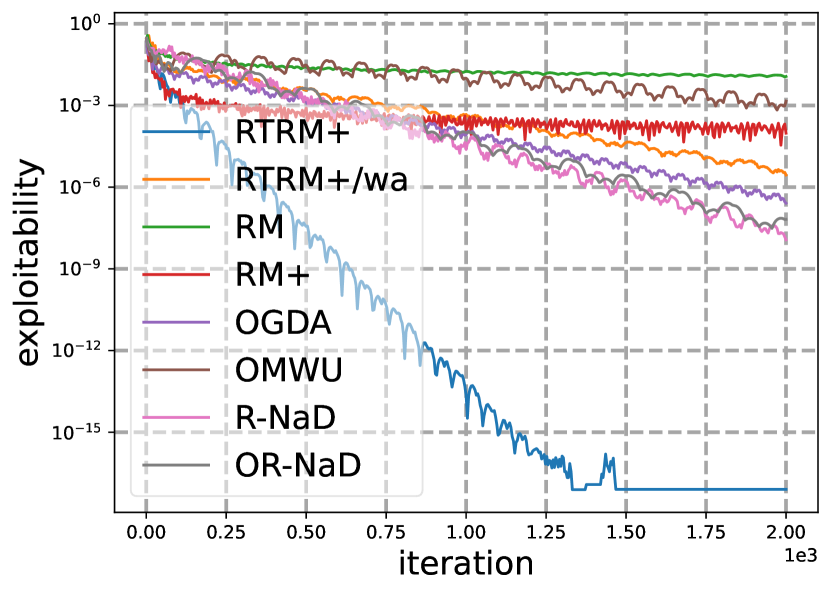
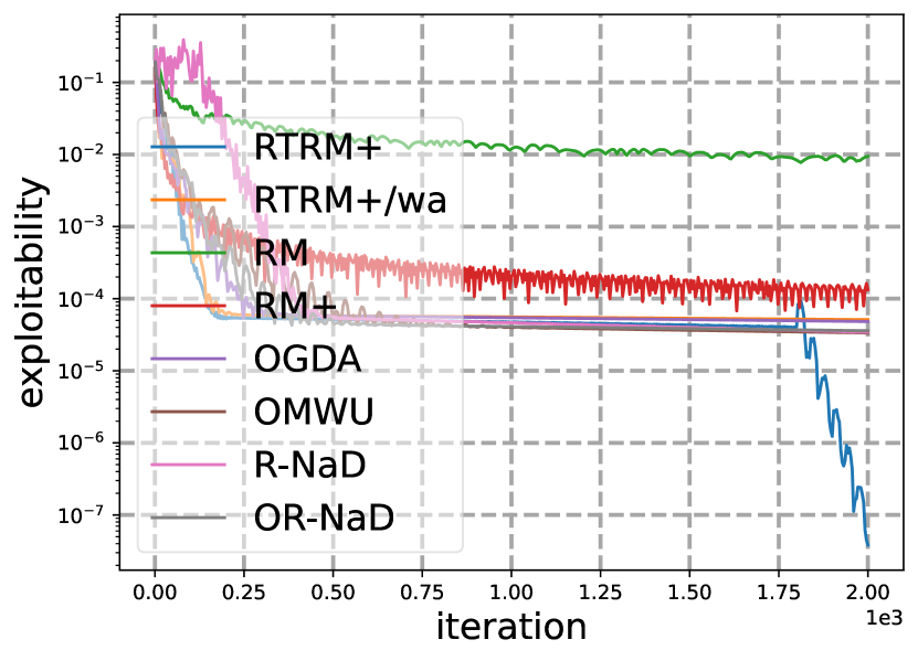
Figure 1: Part of the experimental results in 5x5 NFGs where the seeds are from 0 to 7.

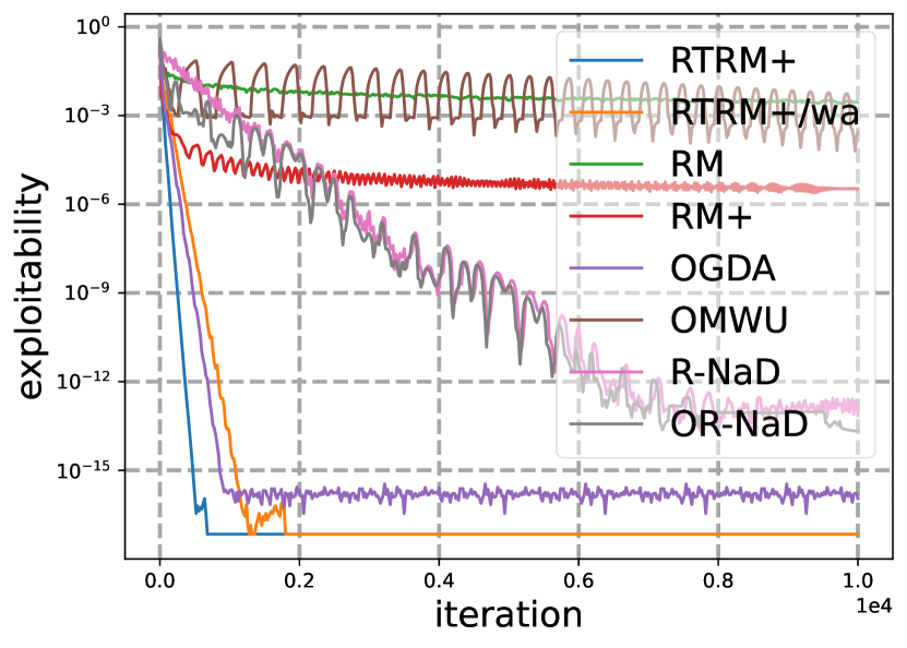
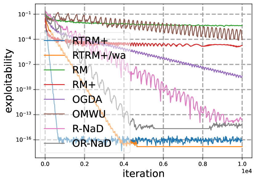
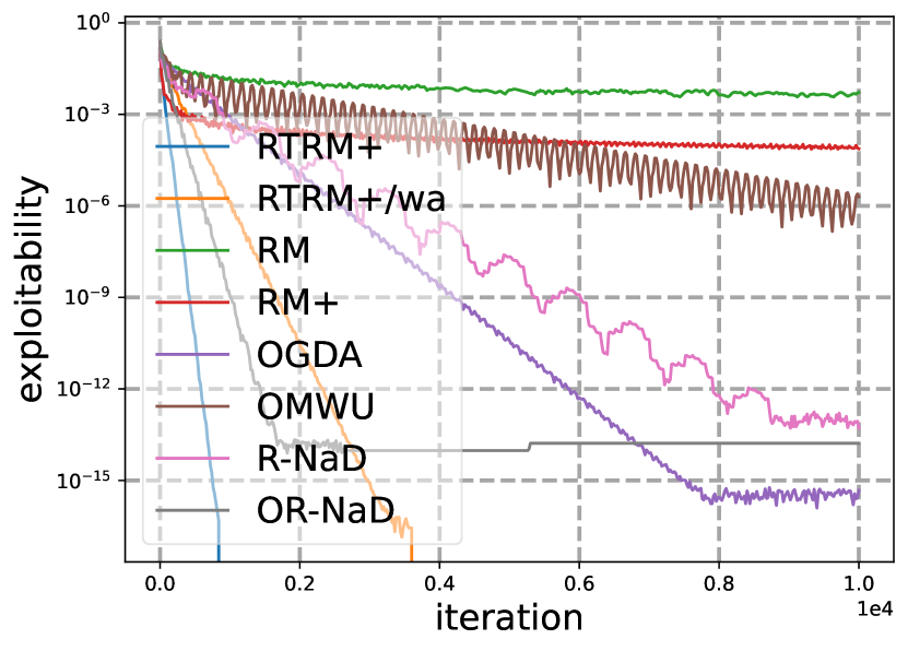
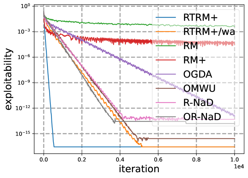
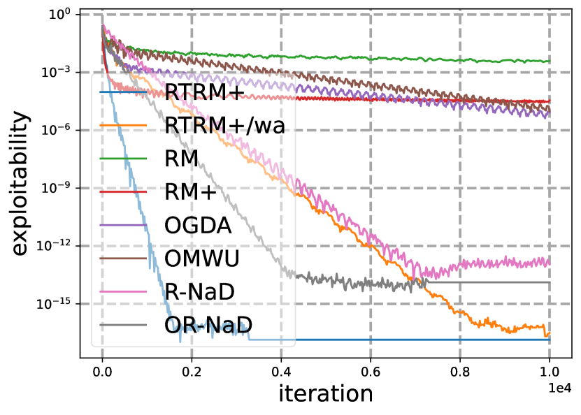
Figure 2: Part of the experimental results in 10x10 NFGs where the seeds are from 0 to 7.

6.2 Evaluation of RTCFR+

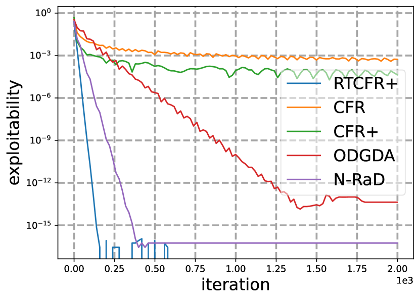
(a) Kuhn Poker

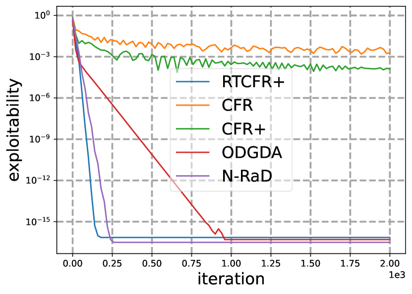
(b) Goofspiel(4)

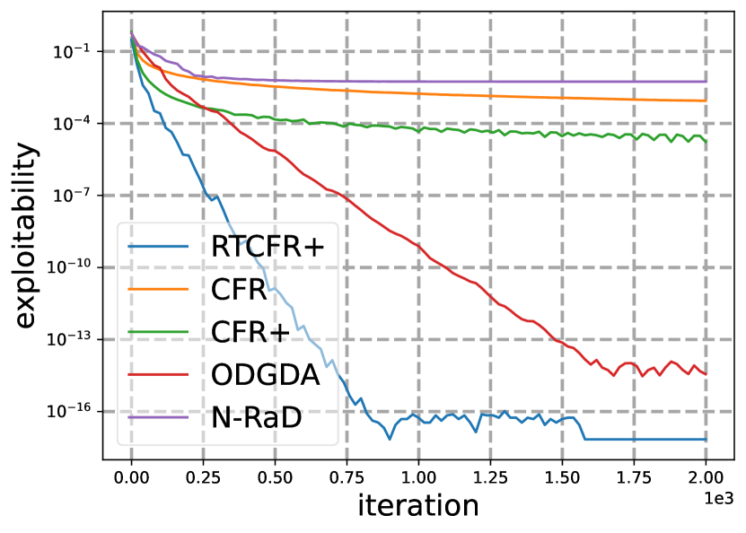
(c) Liars Dice(4)

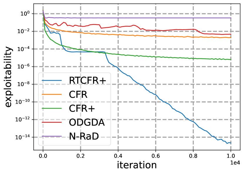
(d) Leduc Poker

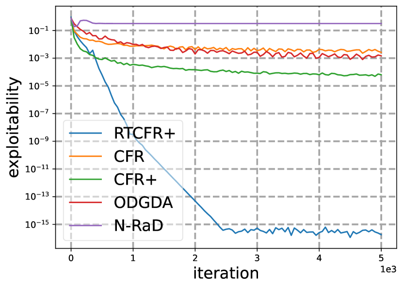
(e) Goofspiel(5)

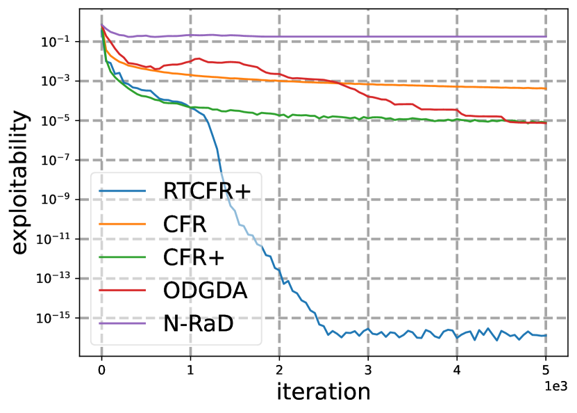
(f) Liars Dice(5)

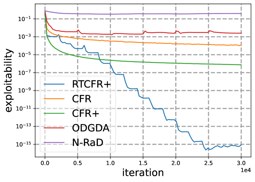
(g) Liars Dice(6)

Figure 3: The experiment results in EFGs. Goofspiel(x) represents the number of cards is x and Liar Dice(x) denotes the side of dice is x. The results are arranged in terms of game size from left to right and top to bottom, i.e., Kuhn Poker is the smallest game, and Liar Dice(6) is the largest game.

Configurations

We evaluate RTCFR+ empirically on four standard EFG benchmarks: Kuhn Poker, Leduc Poker, Goofspiel, and Liar Dice, which are provided by OpenSpiel (Lanctot et al., 2019). We compare RTCFR+ with average-iterate convergence algorithms, such as CFR (Zinkevich et al., 2007) and CFR+ (Bowling et al., 2015), and last-iterate convergence algorithms, such as DOGDA (Farina et al., 2019a; Lee et al., 2021) and R-NaD(Pérolat et al., 2021, 2022). DOGDA is a variant of OGDA that employs the dilated Euclidean square norm (Hoda et al., 2010; Kroer et al., 2015; Farina et al., 2021b) to reduce the computation complexity of OGDA (DOGDA reduces to vanilla OGDA in NFGs). Furthermore, we don’t compare OMWU and OR-NaD since they usually perform worse than OGDA and RTRM+ in NFGs, respectively. RTCFR+, CFR+, and R-NaD use alternating updates. CFR+ also employs linear averaging. We display the performance of the average strategy for CFR and CFR+, while we exhibit the performance of the current strategy for other algorithms. The initial strategy and reference strategy are set up similarly to the experiments on NFGs. More details on the hyperparameters are available in Appendix I.

Results

The results are shown in Figure 3. Although existing last-iterate convergence algorithms (DOGDA and R-NaD) demonstrate significantly better performance than CFR and CFR+ in games smaller than Leduc Poker, they suffer from a sharp degradation in performance as the size of the game increases. In contrast, our algorithm, RTCFR+, demonstrates excellent performance in all tested games in terms of the empirical convergence rate and the final exploitability. For example, the final exploitability obtained by RTCFR+ is $10^{8}$ times lower than CFR+ in all tested games! To our knowledge, RTCFR+ is the first last-iterate convergence algorithm that outperforms CFR+ in EFGs of size larger or equal to Leduc Poker.

7 Conclusion and Future Work

In this paper, we illustrate the essence of the Reward Transformation (RT) framework and identify the bottleneck of this framework. Based on this, we propose RTRM+ and RTCFR+, designed to learn NE in NFGs and EFGs, respectively. The experimental results demonstrate that RTRM+ and RTCFR+ significantly outperform existing last-iterate convergence algorithms and RM+ (CFR+).

While our algorithms exhibit promising empirical performance in both NFGs and EFGs, it is imperative to note that further research is necessary to establish their explicit theoretical convergence rate. In addition, our algorithm is based on the full-feedback assumption. This assumption involves traversing the entire game tree, which is impossible in most real-world games. Therefore, further research is needed to extend our algorithms to the bandit-feedback setting. Lastly, though we have examined the regularizer employed in previous studies and found a new regularizer that can be used in the RT framework, how to design $\phi(\cdot)$ to satisfy Theorem 4.3 remains a problem that requires to be addressed in the future.

Appendix A Counterfactual Regret Decomposition Framework

The counterfactual regret decomposition framework is designed for addressing two-player zero-sum EFGs. Unlike other no-regret algorithms that directly minimize the regret over sequence-form strategy polytope (treeplex) [Hoda et al., 2010], This framework decomposes the regret into each inforset and minimizes the regret over simplex with RM or RM+ [Bowling et al., 2015].

CFR computes the counterfactual value at each inforset $I$ for player $i$

$$q^{\sigma^{t}}(I)=\sum_{z\in\mathcal{Z}}\pi^{\sigma^{t}}_{-i}(I)\pi^{\sigma^{t}}(I,z)u_{i}(z).$$ (10)

Similarly, for each inforset-action pair $(I,a)$, we have

$$q^{\sigma^{t}}(I,a)=\sum_{z\in\mathcal{Z}}\pi^{\sigma^{t}}_{-i}(I)\pi^{\sigma^{t}}(Ia,z)u_{i}(z).$$ (11)

Then we have the instantaneous regret $r^{t}(I,a)$ which is the difference between the counterfactual value of $(I,a)$ with $(I)$

$$r^{t}(I,a)=q^{\sigma^{t}}(I,a)-q^{\sigma^{t}}(I).$$ (12)

Then the counterfactual regret for sequence $(I,a)$ at iteration $t$ is

$$R^{t}(I,a)=\sum_{\tau=1}^{t}r^{\tau}(I,a).$$ (13)

In addition, $R^{T}(I)=\max_{a\in A(I)}R^{T}(I,a)$. It has been proven in  Zinkevich et al. [2007] that the regret of player $i$ over treeplex $R^{T}=\sum_{i\in\{0,1\}}\sum^{T}_{t=1}\max_{\sigma_{i}}u_{i}(\sigma_{i},\sigma^{t}_{-i})-u_{i}(\sigma^{t}_{i},\sigma^{t}_{-i})$ less the sum of the counterfactual regret at each inforset. Formally, $R^{T}\leq\sum_{I\in\mathcal{I}_{i}}R^{T}(I)$. So counterfactual regret decomposition framework can use any regret minimization method to minimize the regret $R^{T}(I)$ over each inforset to minimize the regret $R^{T}$. Among all regret minimizers, RM+ achieves the SOTA empirical performance, which is defined as:

$$Q^{t+1}(I,a) =\max(Q^{t}(I,a)+r^{t}(I,a),0)$$ (14)

$$\sigma^{t+1}(I,a) =\frac{\max(0,Q^{t}(I,a))}{\sum_{a^{\prime}\in A(I)}\max(0,Q^{t}(I,a^{\prime}))}.$$

Appendix B Proof of Theorem 4.3

In this section, we prove Theorem 4.3 holds if Lemma 4.1 and Lemma 4.2 hold.

Proof.

We assume that the set $\mathcal{Z}^{\prime}\cap\mathcal{Z}^{*}$ is not empty. From Lemma 4.1 and the fact that $\min_{\sigma^{*}\in\mathcal{Z}^{*}}D_{\psi}(\sigma^{*},\sigma^{r,n})$, is bounded below by zero, the sequence of $\min_{\sigma^{*}\in\mathcal{Z}^{*}}D_{\psi}(\sigma^{*},\sigma^{r,n})$ converges to $b\geq 0$. In the following, we show that $b=0$ by contradiction.

Suppose that $b>0$. Given a constant $c$, we define $\Omega_{e}=\{\sigma\in\mathcal{Z}|\min_{\sigma^{*}\in\mathcal{Z}^{*}}D_{\psi}(\sigma^{*},\sigma)\leq e\}$ and $\bar{\Omega}_{e}=\{\sigma\in\mathcal{Z}|\min_{\sigma^{*}\in\mathcal{Z}^{*}}D_{\psi}(\sigma^{*},\sigma)<e\}$. According to the continuity of $\min_{\sigma^{*}\in\mathcal{Z}^{*}}D_{\psi}(\sigma^{*},\sigma)$, for any given $e$, the set $\Omega_{e}$ is closed and bounded (and $\bar{\Omega}_{e}$ is open and bounded). Thus, $\Omega_{e}$ is a compact set.

Let us define $E=\min_{\sigma^{*}\in\mathcal{Z}^{*}}D_{\psi}(\sigma^{*},\sigma^{r,1})$. If $b>0$, it means that for all $n\geq 1$, $\sigma^{r,n}$ is in $\Omega_{B}\backslash\bar{\Omega}_{B}$. In addition, since $\Omega_{e}$ is closed and bounded and $\bar{\Omega}_{B}$ is open and bounded, we have that $\Omega_{e}\backslash\bar{\Omega}_{B}$ is a compact set.

Furthermore, from Lemma 4.2, we get that $\min_{\sigma^{*}\in\mathcal{Z}^{*}}D_{\psi}(\sigma^{*},F(\sigma^{r,n}))-\min_{\sigma^{*}\in\mathcal{Z}^{*}}D_{\psi}(\sigma^{*},\sigma^{r,n})$ is a continuous function. Since a continuous function has a maximum over a compact set, the maximum $\nu=\max_{\sigma^{r}\in\Omega_{B}\backslash\bar{\Omega}_{B}}\{\min_{\sigma^{*}\in\mathcal{Z}^{*}}D_{\psi}(\sigma^{*},F(\sigma^{r}))-\min_{\sigma^{*}\in\mathcal{Z}^{*}}D_{\psi}(\sigma^{*},\sigma^{r})\}$. From Lemma 4.1, we have $\nu<0$. Therefore, we get:

$$\min_{\sigma^{*}\in\mathcal{Z}^{*}}D_{\psi}(\sigma^{*},\sigma^{r,n})) =\min_{\sigma^{*}\in\mathcal{Z}^{*}}D_{\psi}(\sigma^{*},\sigma^{r,1})+\sum_{n=1}^{N}\left(\min_{\sigma^{*}\in\mathcal{Z}^{*}}D_{\psi}(\sigma^{*},\sigma^{r,n+1}))-\min_{\sigma^{*}\in\mathcal{Z}^{*}}D_{\psi}(\sigma^{*},\sigma^{r,n})\right)$$ (15)

$$\leq B+\sum_{n=1}^{N}\nu.$$

This contradicts the fact that $b>0$ since there exists $n$ such that $B+\sum_{n=1}^{N}\nu\leq 0$. Therefore, we complete the proof. ∎

Appendix C Proof of Theorem 4.4

Proof.

In this section, with a slight abuse of notation, we directly use $\sigma$ to represent the sequence-form strategy [Von Stengel, 1996, Hoda et al., 2010] despite $\sigma$ denoting the behavioral strategy in the main text. Note that this abuse only affects EFGs since the sequence-form strategy and the behavioral strategy are the same in NFGs. The proof is from the definition of exploitability. Especially, as shown in the following:

$$2\varepsilon(\sigma)= \sum_{i\in\{0,1\}}\max_{\sigma_{-i}^{\prime}}u_{-i}(\sigma_{i},\sigma_{-i}^{\prime})$$ (16)

$$= \sum_{i\in\{0,1\}}\max_{\sigma_{i}\in\Delta(A_{i})}\langle\bm{g}^{t,n}_{i},\sigma^{t,n}_{i}-\sigma_{i}\rangle$$

$$= \sum_{i\in\{0,1\}}\max_{\sigma_{i}\in\Delta(A_{i})}\langle\bm{g}^{*,n}_{i},\bm{g}^{*,n}_{i}-\sigma_{i}\rangle+\sum_{i\in\{0,1\}}\max_{\sigma_{i}\in\Delta(A_{i})}\langle\bm{g}^{t,n}_{i},\sigma^{t,n}_{i}-\sigma_{i}\rangle$$

$$\quad-\sum_{i\in\{0,1\}}\max_{\sigma_{i}\in\Delta(A_{i})}\langle\bm{g}^{*,n}_{i},\sigma^{*,n}_{i}-\sigma_{i}\rangle$$

$$= \quad 2\varepsilon(\sigma^{*,n})+\sum_{i\in\{0,1\}}\max_{\sigma_{i}\in\Delta(A_{i})}\langle\bm{g}^{*,n}_{i}-\bm{g}^{t,n}_{i},\sigma_{i}\rangle$$

$$= \quad 2\varepsilon(\sigma^{*,n})+\sum_{i\in\{0,1\}}\max_{\sigma_{i}\in\Delta(A_{i})}\langle\sigma^{*,n}_{i}-\sigma^{t,n}_{i},-\bm{g}^{\sigma}_{i}\rangle$$

$$\leq \quad 2\varepsilon(\sigma^{*,n})+\mu L\sum_{i\in\{0,1\}}||\sigma^{*,n}_{i}-\sigma^{t,n}_{i}||_{2}$$

$$= \quad 2\varepsilon(\sigma^{*,n})+\mu L||\sigma^{*,n}-\sigma^{t,n}||_{2},$$

where $L=\max_{i,\sigma}\|\bm{g}^{\sigma}_{i}\|_{2}$. ∎

Appendix D Proof of Theorem 5.1

In this section, we prove that if $\varphi(\cdot)$ and $\psi(\cdot)$ are the Euclidean square norm and $\phi(\sigma_{i},\sigma^{r}_{i})=D_{\varphi}(\sigma_{i},\sigma^{r}_{i})$, then Lemma 4.1 and Lemma 4.2 hold. In other words, we prove the following two Lemmas:

Lemma D.1.

Let $\varphi(\cdot)$ and $\psi(\cdot)$ are the Euclidean square norm and $\phi(\sigma_{i},\sigma^{r,n}_{i})=D_{\varphi}(\sigma_{i},\sigma^{r,n}_{i})$, then Lemma 4.1 holds.

Lemma D.2.

Let $\varphi(\cdot)$ and $\psi(\cdot)$ are the Euclidean square norm and $\phi(\sigma_{i},\sigma^{r,n}_{i})=D_{\varphi}(\sigma_{i},\sigma^{r,n}_{i})$, then Lemma 4.2 holds.

D.1 Proof of Lemma D.1

Proof.

Let $\sigma^{*,n}$ be the saddle point of the $n$-th SCCP $\sigma^{*,n}$, for all $i\in\{0,1\}$ and $\sigma^{*}\in\mathcal{Z}^{*}$. Assuming $\sigma^{*,n}\neq\sigma^{r,n}$, we have:

$$\underbrace{\langle\sigma^{*,n}_{i},\bm{\ell}^{*,n}_{i}\rangle}_{{\rm term}\ (b)}=\underbrace{\langle\sigma^{*}_{i},\bm{\ell}^{*,n}_{i}\rangle}_{{\rm term}\ (c)}+\underbrace{\langle\sigma^{*,n}_{i},\bm{\ell}^{*,n}_{i}\rangle-\langle\sigma^{*}_{i},\bm{\ell}^{*,n}_{i}\rangle}_{{\rm term}\ (a)},$$ (17)

where $\bm{\ell}^{*,n}_{i}=\bm{g}^{*,n}_{i}+\mu\nabla\varphi(\sigma^{*,n}_{i})-\mu\nabla\varphi(\sigma^{r,n}_{i})$. From the definition of $\sigma^{*,n}$, for all $\sigma_{i}\in\Delta(A_{i})$, we have:

$$\langle\sigma_{i},\bm{\ell}^{*,n}_{i}\rangle\geq\langle\sigma^{*,n}_{i},\bm{\ell}^{*,n}_{i}\rangle.$$ (18)

Hence, For term ($a$), we get:

$${\rm term}\ (a)=\langle\sigma^{*,n}_{i},\bm{\ell}^{*,n}_{i}\rangle-\langle\sigma^{*}_{i},\bm{\ell}^{*,n}_{i}\rangle\leq 0.$$ (19)

For term ($b$), we have:

$${\rm term}\ (b) =\langle\sigma^{*,n}_{i},\bm{g}^{*,n}_{i}+\mu\nabla\varphi(\sigma^{*,n}_{i})-\mu\nabla\varphi(\sigma^{r,n}_{i})\rangle$$ (20)

$$=-v_{i}^{\sigma^{*,n}}+\mu\langle\sigma^{*,n}_{i},\nabla\varphi(\sigma^{*,n}_{i})-\nabla\varphi(\sigma^{r,n}_{i})\rangle.$$

Finally, For term ($c$), we have:

$${\rm term}\ (c)=\langle\sigma^{*}_{i},\bm{\ell}^{*,n}_{i}\rangle=-v_{i}^{\sigma^{*}_{i},\sigma^{*,n}_{-i}}+\mu\langle\sigma^{*},\nabla\varphi(\sigma^{*,n}_{i})-\nabla\varphi(\sigma^{r,n}_{i})\rangle.$$ (21)

combining Eq. (19), Eq. (20), and Eq. (21),

$$-v_{i}^{\sigma^{*,n}}+\mu\langle\sigma^{*,n}_{i},\nabla\varphi(\sigma^{*,n}_{i})-\nabla\varphi(\sigma^{r,n}_{i})\rangle \leq-v_{i}^{\sigma^{*}_{i},\sigma^{*,n}_{-i}}+\mu\langle\sigma^{*}_{i},\nabla\varphi(\sigma^{*,n}_{i})-\nabla\varphi(\sigma^{r,n}_{i})\rangle.$$ (22)

Then, we get:

$$\mu\sum_{i\in\{0,1\}}\langle\sigma^{*,n}_{i},\nabla\varphi(\sigma^{*,n}_{i})-\nabla\varphi(\sigma^{r,n}_{i})\rangle$$ (23)

$$\leq \sum_{i\in\{0,1\}}-v_{i}^{\sigma^{*}_{i},\sigma^{*,n}_{-i}}+\mu\sum_{i\in\{0,1\}}\langle\sigma^{*}_{i},\nabla\varphi(\sigma^{*,n}_{i})-\nabla\varphi(\sigma^{r,n}_{i})\rangle$$

$$\leq \sum_{i\in\{0,1\}}(v_{i}^{\sigma^{*}}-v_{i}^{\sigma^{*}_{i},\sigma^{*,n}_{-i}})+\mu\sum_{i\in\{0,1\}}\langle\sigma^{*}_{i},\nabla\varphi(\sigma^{*,n}_{i})-\nabla\varphi(\sigma^{r,n}_{i})\rangle$$

$$\leq \mu\sum_{i\in\{0,1\}}\langle\sigma^{*}_{i},\nabla\varphi(\sigma^{*,n}_{i})-\nabla\varphi(\sigma^{r,n}_{i})\rangle,$$

where the second inequality comes from that $\sum_{i\in\{0,1\}}(v_{i}^{\sigma^{*}}-v_{i}^{\sigma^{*}_{i},\sigma^{*,n}_{-i}})\leq 0$. From the above equation, we derive that:

$$\langle\sigma^{*,n},\nabla\varphi(\sigma^{*,n})-\nabla\varphi(\sigma^{r,n})\rangle\leq\langle\sigma^{*},\nabla\varphi(\sigma^{*,n})-\nabla\varphi(\sigma^{r,n})\rangle$$ (24)

$$\Leftrightarrow -\langle\nabla\varphi(\sigma^{*,n}),\sigma^{*}-\sigma^{*,n}\rangle\leq-\langle\nabla\varphi(\sigma^{r,n}),\sigma^{*}-\sigma^{r,n}\rangle+\langle\nabla\varphi(\sigma^{r,n}),\sigma^{*,n}-\sigma^{r,n}\rangle$$

$$\Leftrightarrow D_{\psi}(\sigma^{*},\sigma^{*,n})\leq D_{\psi}(\sigma^{*},\sigma^{r,n})-D_{\psi}(\sigma^{*,n},\sigma^{r,n})$$

$$\Leftrightarrow D_{\psi}(\sigma^{*},\sigma^{*,n})<D_{\psi}(\sigma^{*},\sigma^{r,n})$$

$$\Leftrightarrow D_{\psi}(\sigma^{*},\sigma^{r,n+1})<D_{\psi}(\sigma^{*},\sigma^{r,n}),$$

where the fourth line is from the assumption $\sigma^{*,n}\neq\sigma^{r,n}$ that $D_{\psi}(\sigma^{*,n},\sigma^{r,n})>0$ which the equality holds if and only if $\sigma^{*,n}=\sigma^{r,n}$.

Now assuming $\sigma^{*,n}=\sigma^{r,n}$, for all $\sigma_{i}\in\Delta(A_{i})$, we have:

$$\langle\sigma_{i},\bm{\ell}^{*,n}_{i}\rangle\geq\langle\sigma^{*,n}_{i},\bm{\ell}^{*,n}_{i}\rangle$$ (25)

$$\Leftrightarrow \langle\sigma_{i},\bm{g}^{*,n}_{i}+\mu\nabla\varphi(\sigma^{*,n}_{i})-\mu\nabla\varphi(\sigma^{r,n}_{i})\rangle\geq\langle\sigma^{*,n}_{i},\bm{g}^{*,n}_{i}+\mu\nabla\varphi(\sigma^{*,n}_{i})-\mu\nabla\varphi(\sigma^{r,n}_{i})\rangle,$$

with the assumption $\sigma^{*,n}=\sigma^{r,n}$, we have:

$$\langle\sigma_{i},\bm{g}^{*,n}_{i}\rangle\geq\langle\sigma^{*,n}_{i},\bm{g}^{*,n}_{i}\rangle.$$ (26)

Thus, from the definition of NE, we have $\sigma^{*,n}\in\mathcal{Z}^{*}$. This completes the proof. ∎

D.2 Proof of Lemma D.1

Proof.

To prove the continuity of the $F(\cdot)$ function, we have to prove that for every $\gamma>0$, there exists $\delta>0$ such that for all $\sigma^{r,n,\prime},\sigma^{r,n}\in\mathcal{Z}$, if $\|\sigma^{r,n,\prime}-\sigma^{r,n}\|_{2}<\delta$, then $\|\sigma^{*,n,\prime}-\sigma^{*,n}\|_{2}<\gamma$, where $\sigma^{*,n,\prime}$ is saddle point if the reference is the $\sigma^{r,n,\prime}$.

We first introduce the following Lemma.

Lemma D.3.

Let $\varphi(\cdot),\psi(\cdot)$ as the Euclidean square norm, $\phi(\sigma_{i},\sigma^{r}_{i})=D_{\varphi}(\sigma_{i},\sigma^{r}_{i})$, $\sigma^{*,r}$ as the saddle point of the built SCCP and $\bm{g}^{*,r}_{i}$ as the loss gradient if opponent follows strategy $\sigma^{*,r}_{-i}$. For any strategy $\sigma\in\mathcal{Z}$ we have:

$$\sum_{i\in\{0,1\}}\langle\sigma_{i},\bm{g}^{*,r}_{i}\rangle\geq\mu\sum_{i\in\{0,1\}}\langle\sigma^{*,r}_{i}-\sigma_{i},\nabla\varphi(\sigma^{*,r}_{i})-\nabla\varphi(\sigma^{r}_{i})\rangle.$$ (27)

Proof.

From the definition of $\sigma^{*,r}$, for all $\sigma_{i}\in\Delta(A_{i})$, we get:

$$\sum_{i\in\{0,1\}}\langle\sigma_{i},\bm{g}^{*,r}_{i}+\mu\nabla\varphi(\sigma^{*,r}_{i})-\mu\nabla\varphi(\sigma^{r}_{i})\rangle\geq\sum_{i\in\{0,1\}}\langle\sigma^{*,r}_{i},\bm{g}^{*,r}_{i}+\mu\nabla\varphi(\sigma^{*,r}_{i})-\mu\nabla\varphi(\sigma^{r}_{i})\rangle$$ (28)

$$\Leftrightarrow \sum_{i\in\{0,1\}}\langle\sigma_{i},\bm{g}^{*,r}_{i}\rangle\geq\mu\sum_{i\in\{0,1\}}\langle\sigma^{*,r}_{i}-\sigma_{i},\nabla\varphi(\sigma^{*,r}_{i})-\nabla\varphi(\sigma^{r}_{i})\rangle,$$

where the second line comes from $\sum_{i\in\{0,1\}}\langle\bm{g}^{*,r}_{i},\sigma^{*,r}_{i}\rangle=0$. ∎

From the definition of $\sigma^{*,n}$, we have:

$$0\leq\langle\bm{g}^{*,n}_{i}+\mu\nabla\varphi(\sigma^{*,n}_{i})-\mu\nabla\varphi(\sigma^{r,n}_{i}),\sigma^{*,n,\prime}_{i}-\sigma^{*,n}\rangle.$$ (29)

Thus, we have:

$$0\leq \underbrace{\sum_{i\in\{0,1\}}\langle\bm{g}^{*,n}_{i}+\mu\nabla\varphi(\sigma^{*,n}_{i})-\mu\nabla\varphi(\sigma^{r,n,\prime}_{i}),\sigma^{*,n,\prime}_{i}-\sigma^{*,n}\rangle}_{{\rm term}\ (a)}+\underbrace{\sum_{i\in\{0,1\}}\langle\mu\nabla\varphi(\sigma^{r,n,\prime}_{i})-\mu\nabla\varphi(\sigma^{r,n}_{i}),\sigma^{*,n,\prime}_{i}-\sigma^{*,n}_{i}\rangle}_{{\rm term}\ (b)}.$$ (30)

For term ($a$), we have:

$$\sum_{i\in\{0,1\}}\langle\bm{g}^{*,n}_{i}+\mu\nabla\varphi(\sigma^{*,n}_{i})-\mu\nabla\varphi(\sigma^{r,n,\prime}_{i}),\sigma^{*,n,\prime}_{i}-\sigma^{*,n}\rangle$$ (31)

$$= \sum_{i\in\{0,1\}}\langle\bm{g}^{*,n}_{i},\sigma^{*,n,\prime}_{i}\rangle+\mu\sum_{i\in\{0,1\}}\langle\nabla\varphi(\sigma^{*,n}_{i})-\nabla\varphi(\sigma^{r,n,\prime}_{i}),\sigma^{*,n,\prime}_{i}-\sigma^{*,n}\rangle$$

$$= \sum_{i\in\{0,1\}}-\langle\bm{g}^{*,n,\prime}_{i},\sigma^{*,n}_{i}\rangle+\mu\sum_{i\in\{0,1\}}\langle\nabla\varphi(\sigma^{*,n}_{i})-\nabla\varphi(\sigma^{r,n,\prime}_{i}),\sigma^{*,n,\prime}_{i}-\sigma^{*,n}\rangle$$

$$\leq -\mu\sum_{i\in\{0,1\}}\langle\nabla\varphi(\sigma^{*,n,\prime}_{i})-\nabla\varphi(\sigma^{r,n,\prime}_{i}),\sigma^{*,n,\prime}_{i}-\sigma^{*,n}_{i}\rangle+\mu\sum_{i\in\{0,1\}}\langle\nabla\varphi(\sigma^{*,n}_{i})-\nabla\varphi(\sigma^{r,n,\prime}_{i}),\sigma^{*,n,\prime}_{i}-\sigma^{*,n}\rangle$$

$$= \mu\sum_{i\in\{0,1\}}\langle\nabla\varphi(\sigma^{*,n,\prime}_{i})-\nabla\varphi(\sigma^{*,n}_{i}),\sigma^{*,n}_{i}-\sigma^{*,n,\prime}_{i}\rangle$$

$$= -\mu\|\sigma^{*,n,\prime}-\sigma^{*,n}\|^{2}_{2},$$

where the fourth line comes from Lemma D.3. In addition, For term ($b$), we get:

$$\sum_{i\in\{0,1\}}\langle\mu\nabla\varphi(\sigma^{r,n,\prime}_{i})-\mu\nabla\varphi(\sigma^{r,n}_{i}),\sigma^{*,n,\prime}_{i}-\sigma^{*,n}_{i}\rangle$$ (32)

$$\leq \mu\sum_{i\in\{0,1\}}\|\sigma^{r,n,\prime}_{i}-\sigma^{r,n}_{i}\|_{2}\|\sigma^{*,n,\prime}_{i}-\sigma^{*,n}_{i}\|_{2}$$

$$\leq \mu\|\sigma^{r,n,\prime}-\sigma^{r,n}\|_{2},$$

where the second line comes from $\|\sigma^{*,n,\prime}-\sigma^{*,n}\|_{2}\leq 1$. Combining Eq. (30), (31) and (32), we get:

$$\|\sigma^{*,n,\prime}-\sigma^{*,n}\|^{2}_{2}\leq\|\sigma^{r,n,\prime}-\sigma^{r,n}\|_{2}$$ (33)

$$\Leftrightarrow \|\sigma^{*,n,\prime}-\sigma^{*,n}\|_{2}\leq\sqrt{\|\sigma^{r,n,\prime}-\sigma^{r,n}\|_{2}}.$$

From the assumption that $\|\sigma^{r,n,\prime}-\sigma^{r,n}\|_{2}\leq\delta$, we have $\|\sigma^{*,n,\prime}-\sigma^{*,n}\|_{2}\leq\sqrt{\delta}$. This completes the proof.

∎

Appendix E Proof of Theorem 5.2

Proof.

To prove Theorem 5.2, we first introduce the following Lemmas to enable the dynamics of RM+ can be represented via the Online Mirror Descent form.

Lemma E.1.

[Farina et al., 2021a] Regret matching+ (Eq.(8)) update is equivalent to the following update

$$\bm{\theta}^{t+1,n}_{i}\in\mathop{\arg min}\limits_{\bm{\theta}_{i}\in R^{d}_{\geq 0}}\{\langle-\bm{m}_{i}(\bm{\theta}^{t,n}),\bm{\theta}_{i}\rangle+\frac{1}{\eta}D_{\psi}(\bm{\theta}_{i},\bm{\theta}^{t,n}_{i})\}$$ (34)

where $\eta$ is a constant, $d=|A_{i}|$, $\frac{\bm{\theta}^{t+1,n}_{i}}{\|\bm{\theta}^{t+1,n}_{i}\|_{1}}=\frac{Q^{t,n}_{i}}{\|Q^{t,n}_{i}\|_{1}}$, $\bm{m}_{i}(\bm{\theta}^{t,n})=\langle\bm{\ell}^{t,n}_{i},\sigma^{t,n}_{i}\rangle\bm{1}-\bm{\ell}^{t,n}_{i}$, $\bm{\ell}^{t,n}_{i}=\bm{g}^{t,n}_{i}+\mu\sigma^{t,n}_{i}-\mu\sigma^{r,n}_{i}$, $\bm{g}^{t,n}_{i}=\left[-\sum_{a_{-i}\in A_{-i}}\sigma^{t,n}_{-i}(a_{-i})u_{i}(a_{i},a_{-i})\right]_{a_{i}\in A_{i}}$ is the loss gradient at iteration $t$ of the $n$-th SCCP, and $\psi(\cdot)$ is the Euclidean square norm.

The update rule shown in Eq.(34) has a closed-form solution that $\bm{\theta}^{t+1,n}_{i}=\max(\bm{\theta}^{t,n}_{i}+\eta\bm{m}_{i}(\bm{\theta}^{t,n}),0)$. With the first-order optimality condition of $\bm{\theta}^{t+1,n}_{i}$, for any $\bm{\theta}_{i}\in R^{d}_{\geq 0}$, we have:

$$\langle-\bm{m}_{i}(\bm{\theta}^{t,n})+\frac{1}{\eta}\bm{\theta}^{t+1,n}_{i}-\frac{1}{\eta}\bm{\theta}^{t,n}_{i},\bm{\theta}^{t}_{i}-\bm{\theta}^{t+1,n}_{i}\rangle$$ (35)

$$\Leftrightarrow \langle-\bm{m}_{i}(\bm{\theta}^{t,n}),\bm{\theta}_{i}-\bm{\theta}^{t+1,n}_{i}\rangle+\frac{1}{\eta}\langle\bm{\theta}^{t+1,n}_{i}-\bm{\theta}^{t,n}_{i},\bm{\theta}^{t,n}_{i}-\bm{\theta}^{t+1,n}_{i}\rangle\geq\frac{1}{\eta}\langle\bm{\theta}^{t+1,n}_{i}-\bm{\theta}^{t,n}_{i},\bm{\theta}^{t,n}_{i}-\bm{\theta}_{i}\rangle.$$

In addition, from the definition of Euclidean square norm, for any $\bm{\theta}_{i}\in R^{d}_{\geq 0}$, we get:

$$D_{\psi}(\bm{\theta}_{i},\bm{\theta}^{t+1,n}_{i})-D_{\psi}(\bm{\theta}_{i},\bm{\theta}^{t,n}_{i})=D_{\psi}(\bm{\theta}^{t,n}_{i},\bm{\theta}^{t+1,n}_{i})+\langle\bm{\theta}^{t+1,n}_{i}-\bm{\theta}^{t,n}_{i},\bm{\theta}^{t,n}_{i}-\bm{\theta}_{i}\rangle.$$ (36)

Combing Eq. (35) and (36), we have:

$$D_{\psi}(\bm{\theta}_{i},\bm{\theta}^{t+1,n}_{i})\leq D_{\psi}(\bm{\theta}_{i},\bm{\theta}^{t,n}_{i})+D_{\psi}(\bm{\theta}^{t,n}_{i},\bm{\theta}^{t+1,n}_{i})+\eta\langle-\bm{m}_{i}(\bm{\theta}^{t,n}),\bm{\theta}_{i}-\bm{\theta}^{t+1,n}_{i}\rangle-2D_{\psi}(\bm{\theta}^{t,n}_{i},\bm{\theta}^{t+1,n}_{i})$$ (37)

$$\leq D_{\psi}(\bm{\theta}_{i},\bm{\theta}^{t,n}_{i})-D_{\psi}(\bm{\theta}^{t,n}_{i},\bm{\theta}^{t+1,n}_{i})+\eta\langle-\bm{m}_{i}(\bm{\theta}^{t,n}),\bm{\theta}_{i}-\bm{\theta}^{t+1,n}_{i}\rangle.$$

Substituting $\bm{\theta}^{t,n,*}=[\bm{\theta}_{0}^{t,n,*};\bm{\theta}_{1}^{t,n,*}]\in\arg\min_{\bm{\theta}\in\{k*[\sigma^{*,n}_{0};\sigma^{*,n}_{1}]:\sigma^{*}\in\mathcal{Z}^{*},k\geq 1\}}D_{\psi}(\bm{\theta},\bm{\theta}^{t,n})$ into Eq. (37), we get:

$$D_{\psi}(\bm{\theta}^{t,n,*},\bm{\theta}^{t+1,n})\leq D_{\psi}(\bm{\theta}^{t,n,*},\bm{\theta}^{t,n})-D_{\psi}(\bm{\theta}^{t,n},\bm{\theta}^{t+1,n})+\eta\langle-\bm{m}(\bm{\theta}^{t,n}),\bm{\theta}^{t,n,*}-\bm{\theta}^{t+1,n}\rangle,$$ (38)

where $\bm{\theta}=[\bm{\theta}_{0};\bm{\theta}_{1}]$. Therefore, we have:

$$D_{\psi}(\bm{\theta}^{t,n,*},\bm{\theta}^{t+1,n})+\eta\langle-\bm{m}(\bm{\theta}^{t,n,*}),\bm{\theta}^{t+1,n})\rangle-D_{\psi}(\bm{\theta}^{t,n,*},\bm{\theta}^{t,n})-\eta\langle-\bm{m}(\bm{\theta}^{t,n,*}),\bm{\theta}^{t,n})\rangle$$ (39)

$$\leq -D_{\psi}(\bm{\theta}^{t,n},\bm{\theta}^{t+1,n})+\underbrace{\eta\langle\bm{m}(\bm{\theta}^{t,n,*})-\bm{m}(\bm{\theta}^{t,n}),\bm{\theta}^{t,n}-\bm{\theta}^{t+1,n}\rangle}_{{\rm term}\ (a)}+\underbrace{\eta\langle-\bm{m}(\bm{\theta}^{t,n}),\bm{\theta}^{t,n,*})\rangle}_{{\rm term}\ (b)},$$

where $\bm{m}(\cdot)=[\bm{m}_{0}(\cdot);\bm{m}_{1}(\cdot)]$ and the right hand comes from that $\langle\bm{m}_{i}(\bm{\theta}^{t,n}),\bm{\theta}^{t,n}_{i}\rangle=0$. For term ($a$), we have:

$$\eta\langle\bm{m}(\bm{\theta}^{t,n,*})-\bm{m}(\bm{\theta}^{t,n}),\bm{\theta}^{t,n}-\bm{\theta}^{t+1,n}\rangle\leq\eta\|\bm{m}(\bm{\theta}^{t,n,*})-\bm{m}(\bm{\theta}^{t,n})\|_{2}\|\bm{\theta}^{t,n}-\bm{\theta}^{t+1,n}\|_{2}.$$ (40)

Lemma E.2.

For any $\theta,\theta^{\prime}\in R^{|A_{0}|+|A_{1}|}_{\geq 0}$, we have:

$$\|\bm{m}(\theta)-\bm{m}(\theta^{\prime})\|_{2}\leq C_{0}\|\sigma-\sigma^{\prime}\|_{2},$$ (41)

where $\sigma=[\sigma_{0};\sigma_{1}]$, $\sigma_{i}=\frac{\theta_{i}}{\|\theta_{i}\|_{1}}$, $\sigma^{\prime}_{i}=\frac{\theta^{\prime}_{i}}{\|\theta^{\prime}_{i}\|_{1}}$ and $C_{0}=2P^{2}+3\mu P+P+\mu$.

Then, combing Lemma E.2 and Eq. (40), we get:

$$\eta\langle\bm{m}(\bm{\theta}^{t,n,*})-\bm{m}(\bm{\theta}^{t,n}),\bm{\theta}^{t,n}-\bm{\theta}^{t+1,n}\rangle\leq \eta C_{0}\|\sigma^{*,n}-\sigma^{t,n}\|_{2}\|\bm{\theta}^{t,n}-\bm{\theta}^{t+1,n}\|_{2}$$ (42)

$$\leq (\eta C_{0})^{2}D_{\psi}(\sigma^{*,n},\sigma^{t,n})+D_{\psi}(\bm{\theta}^{t,n},\bm{\theta}^{t+1,n})$$

where the second line comes from that $ab\leq\frac{\rho a^{2}}{2}+\frac{b^{2}}{2\rho}\quad\forall\rho\geq 0$. In addition, For term ($b$), we have:

$$\eta\langle-\bm{m}(\bm{\theta}^{t,n}),\bm{\theta}^{t,n,*})\rangle= \sum_{i\in\{0,1\}}\|\bm{\theta}^{t,n,*}_{i}\|_{1}\langle\bm{\ell}^{t,n}_{i},\sigma^{*,n}_{i}-\sigma^{t,n}_{i}\rangle$$ (43)

$$\leq \eta\sum_{i\in\{0,1\}}\|\bm{\theta}^{t,n,*}_{i}\|_{1}\langle\bm{\ell}^{t,n}_{i}-\bm{\ell}^{*,n}_{i},\sigma^{*,n}_{i}-\sigma^{t,n}_{i}\rangle$$

$$\leq \eta\|\bm{\theta}^{t,n,*}_{i}\|_{1}\sum_{i\in\{0,1\}}\langle\bm{\ell}^{t,n}_{i}-\bm{\ell}^{*,n}_{i},\sigma^{*,n}_{i}-\sigma^{t,n}_{i}\rangle$$

$$\leq \eta\|\bm{\theta}^{t,n,*}_{i}\|_{1}\sum_{i\in\{0,1\}}\langle\bm{g}^{t,n}_{i}-\bm{g}^{*,n}_{i},\sigma^{*,n}_{i}-\sigma^{t,n}_{i}\rangle+\mu\langle\sigma^{t,n}_{i}-\sigma^{*,n}_{i},\sigma^{*,n}_{i}-\sigma^{t,n}_{i}\rangle$$

$$\leq \eta\mu\|\bm{\theta}^{t,n,*}_{i}\|_{1}\langle\sigma^{t,n}-\sigma^{*,n},\sigma^{*,n}-\sigma^{t,n}\rangle$$

$$= -2\eta\mu\|\bm{\theta}^{t,n,*}_{i}\|_{1}D_{\psi}(\sigma^{*,n},\sigma^{t,n})\leq-2\eta\mu D_{\psi}(\sigma^{*,n},\sigma^{t,n}),$$

where the second line comes from that $\langle\bm{\ell}^{*,n}_{i},\sigma^{*,n}_{i}-\sigma_{i}\rangle\leq 0$ for all $\sigma_{i}\in\Delta(A_{i})$, the third and last lines comes from the definition of $\bm{\theta}^{t,n,*}_{i}$, and the fifth line follows from $\sum_{i\in\{0,1\}}\langle\bm{g}^{t,n}_{i}-\bm{g}^{*,n}_{i},\sigma^{*,n}_{i}-\sigma^{t,n}_{i}\rangle=0$. Substituting Eq. (42) and (43) into Eq. (39), we get:

$$D_{\psi}(\bm{\theta}^{t,n,*},\bm{\theta}^{t+1,n})+\eta\langle-\bm{m}(\bm{\theta}^{t,n,*}),\bm{\theta}^{t+1,n})\rangle-D_{\psi}(\bm{\theta}^{t,n,*},\bm{\theta}^{t,n})-\eta\langle-\bm{m}(\bm{\theta}^{t,n,*}),\bm{\theta}^{t,n})\rangle$$ (44)

$$\leq -D_{\psi}(\bm{\theta}^{t,n},\bm{\theta}^{t+1,n})+(\eta C_{0})^{2}D_{\psi}(\sigma^{*,n},\sigma^{t,n})+D_{\psi}(\bm{\theta}^{t,n},\bm{\theta}^{t+1,n})-2\eta\mu D_{\psi}(\sigma^{*,n},\sigma^{t,n}).$$

If $\eta<\frac{2\mu}{(C_{0})^{2}}$ and setting $2\eta\mu-(\eta C_{0})^{2}=C_{1}>0$, we have:

$$D_{\psi}(\bm{\theta}^{t,n,*},\bm{\theta}^{t+1,n})+\eta\langle-\bm{m}(\bm{\theta}^{t,n,*}),\bm{\theta}^{t+1,n})\rangle-D_{\psi}(\bm{\theta}^{t,n,*},\bm{\theta}^{t,n})-\eta\langle-\bm{m}(\bm{\theta}^{t,n,*}),\bm{\theta}^{t,n})\rangle$$ (45)

$$\leq -C_{1}D_{\psi}(\sigma^{*,n},\sigma^{t,n}).$$

Setting $\bm{\theta}^{t+1,n,*}=[\bm{\theta}_{0}^{t+1,n,*};\bm{\theta}_{1}^{t+1,n,*}]\in\arg\min_{\bm{\theta}\in\{k*[\sigma^{*,n}_{0};\sigma^{*,n}_{1}]:\sigma^{*}\in\mathcal{Z}^{*},k\geq 1\}}D_{\psi}(\bm{\theta},\bm{\theta}^{t+1,n})$, from the definition of $\bm{\theta}^{t,n,*}$, we have:

$$D_{\psi}(\bm{\theta}^{t,n,*},\bm{\theta}^{t+1,n})\geq D_{\psi}(\bm{\theta}^{t+1,n,*},\bm{\theta}^{t+1,n}).$$ (46)

Furthermore, with the definition of $\bm{m}(\bm{\theta}^{t,n,*})$, we have $\bm{m}(\bm{\theta}^{t,n,*})=\bm{m}(\sigma^{*,n})$. Thus, we get:

$$D_{\psi}(\bm{\theta}^{t+1,n,*},\bm{\theta}^{t+1,n})+\eta\langle-\bm{m}(\sigma^{*,n}),\bm{\theta}^{t+1,n})\rangle-D_{\psi}(\bm{\theta}^{t,n,*},\bm{\theta}^{t,n})-\eta\langle-\bm{m}(\sigma^{*,n}),\bm{\theta}^{t,n})\rangle$$ (47)

$$\leq -C_{1}D_{\psi}(\sigma^{*,n},\sigma^{t,n}).$$

Then, we have:

$$D_{\psi}(\bm{\theta}^{T+1,n,*},\bm{\theta}^{T+1,n})+\eta\langle-\bm{m}(\sigma^{*,n}),\bm{\theta}^{t+1,n})\rangle\leq D_{\psi}(\bm{\theta}^{1,n,*},\bm{\theta}^{1,n})+\eta\langle-\bm{m}(\sigma^{*,n}),\bm{\theta}^{1,n})\rangle$$ (48)

$$-\sum^{T}_{t=1}C_{1}D_{\psi}(\sigma^{*,n},\sigma^{t,n}).$$

From the definition of $\eta\langle-\bm{m}(\sigma^{*,n}),\bm{\theta}^{t+1,n})\rangle$ and $\eta\langle-\bm{m}(\sigma^{*,n}),\bm{\theta}^{t+1,n})\rangle$, we have:

$$\langle-\bm{m}(\sigma^{*,n}),\bm{\theta}^{t+1,n})\rangle\geq 0,\ {\rm and}\ \langle-\bm{m}(\sigma^{*,n}),\bm{\theta}^{t,n})\rangle\geq 0.$$ (49)

Therefore, if $\sum^{T}_{t=1}C_{1}D_{\psi}(\sigma^{t,n},\sigma^{*,n})\leq D_{\psi}(\bm{\theta}^{1,n,*},\bm{\theta}^{1,n})+\eta\langle-\bm{m}(\sigma^{*,n}),\bm{\theta}^{1,n})\rangle=C_{2}$ does not hold, then $D_{\psi}(\bm{\theta}^{T+1,n,*},\bm{\theta}^{T+1,n})+\eta\langle-\bm{m}(\sigma^{*,n}),\bm{\theta}^{t+1,n})\rangle$ will be less than 0, which is contrary to its definition. Thus, we have $\sum^{T}_{t=1}C_{1}D_{\psi}(\sigma^{*,n},\sigma^{t,n})\leq C_{2}$ for any $T$, which implies $\sigma^{t,n}$ converges asymptotically to $\sigma^{*,n}$.

However, we do not need to tune the value of $\eta$. Precisely, the sequence of strategies generated by $\bm{\theta}^{t+1,n}_{i}=\max(\bm{\theta}^{t,n}_{i}+\eta\bm{m}_{i}(\bm{\theta}^{t,n}),0)$ and $\frac{1}{\eta}\bm{\theta}^{t+1,n}_{i}=\max(\frac{1}{\eta}\bm{\theta}^{t,n}_{i}+\bm{m}_{i}(\bm{\theta}^{t,n}),0)$ are the same. If the sequence of strategies is generated by $\frac{1}{\eta}\bm{\theta}^{t+1,n}_{i}=\max(\frac{1}{\eta}\bm{\theta}^{t,n}_{i}+\bm{m}_{i}(\bm{\theta}^{t,n}),0)$, we have $\frac{1}{\eta}\bm{\theta}^{t+1,n}_{i}=Q^{t,n}_{i}$, which implies $\eta=\frac{\bm{\theta}^{t+1,n}_{i}}{Q^{t,n}_{i}}$ holds at each iteration $t$. Therefore, we have $\eta=\frac{\bm{\theta}^{1,n}_{i}}{Q^{0,n}_{i}}$. For any $Q^{0,n}_{i}$, we can set $\bm{\theta}^{1,n}_{i}$ as any vector that satisfy $\eta=\frac{\bm{\theta}^{1,n}_{i}}{Q^{0,n}_{i}}\leq\frac{2\mu}{(C_{0})^{2}}$. In addition, note that $\sum^{T}_{t=1}C_{1}D_{\psi}(\sigma^{*,n},\sigma^{t,n})\leq C_{2}$ holds for any $\bm{\theta}^{1,n}_{i}$. Therefore, for any $Q^{0,n}_{i}$, we have $\sum^{T}_{t=1}C_{1}D_{\psi}(\sigma^{*,n},\sigma^{t,n})\leq C_{2}$. This completes the proof.

∎

E.1 Proof of Lemma E.2

Proof.

From the definition of $\|\bm{m}(\theta)-\bm{m}(\theta^{\prime})\|_{2}$, we have:

$$\|\bm{m}(\theta)-\bm{m}(\theta^{\prime})\|_{2}$$ (50)

$$= \sum_{i\in\{0,1\}}\|\langle\bm{\ell}_{i},\sigma_{i}\rangle\bm{1}-\bm{\ell}_{i}-\langle\bm{\ell}^{\prime}_{i},\sigma^{\prime}_{i}\rangle\bm{1}-\bm{\ell}^{\prime}_{i}\|_{2}$$

$$= \sum_{i\in\{0,1\}}\|\langle\bm{g}_{i},\sigma_{i}\rangle\bm{1}-\langle\bm{g}^{\prime}_{i},\sigma^{\prime}_{i}\rangle\bm{1}+\bm{g}^{\prime}_{i}-\bm{g}_{i}+\mu\langle\sigma_{i},\sigma_{i}\rangle\bm{1}-\mu\langle\sigma^{\prime}_{i},\sigma^{\prime}_{i}\rangle\bm{1}+$$

$$\quad\quad\quad\mu\sigma_{i}-\mu\sigma^{\prime}_{i}+\mu\langle\sigma^{\prime}_{i},\sigma^{r}_{i}\rangle\bm{1}-\mu\langle\sigma_{i},\sigma^{r}_{i}\rangle\bm{1}\|_{2}$$

Then from the definition of $2$-norm, we have:

$$\|\bm{m}(\theta)-\bm{m}(\theta^{\prime})\|_{2}$$ (51)

$$\leq \sum_{i\in\{0,1\}}|A_{i}|\|\langle\bm{g}_{i},\sigma_{i}\rangle-\langle\bm{g}^{\prime}_{i},\sigma^{\prime}_{i}\rangle\|_{2}+\|\bm{g}^{\prime}_{i}-\bm{g}_{i}\|_{2}+\mu|A_{i}|\|\langle\sigma_{i},\sigma_{i}\rangle-\langle\sigma^{\prime}_{i},\sigma^{\prime}_{i}\rangle\|_{2}+$$

$$\quad\quad\quad\mu\|\sigma_{i}-\sigma^{\prime}_{i}\|_{2}+\mu|A_{i}|\|\langle\sigma^{\prime}_{i}-\sigma_{i},\sigma^{r}_{i}\rangle\|_{2}$$

$$\leq \sum_{i\in\{0,1\}}|A_{i}|\|\langle\bm{g}_{i}-\bm{g}^{\prime}_{i},\sigma_{i}\rangle-\langle\bm{g}^{\prime}_{i},\sigma^{\prime}_{i}-\sigma_{i}\rangle\|_{2}+\|\bm{g}^{\prime}_{i}-\bm{g}_{i}\|_{2}+\mu|A_{i}|\|\langle\sigma_{i},\sigma_{i}\rangle-\langle\sigma^{\prime}_{i},\sigma^{\prime}_{i}\rangle\|_{2}+$$

$$\quad\quad\quad\mu\|\sigma_{i}-\sigma^{\prime}_{i}\|_{2}+\mu|A_{i}|\|\langle\sigma^{\prime}_{i}-\sigma_{i},\sigma^{r}_{i}\rangle\|_{2}$$

Then, we have:

$$\|\bm{m}(\theta)-\bm{m}(\theta^{\prime})\|_{2}$$ (52)

$$\leq \sum_{i\in\{0,1\}}|A_{i}|\|\langle\bm{g}_{i}-\bm{g}^{\prime}_{i},\sigma_{i}\rangle\|_{2}+|A_{i}|\|\langle\bm{g}^{\prime}_{i},\sigma^{\prime}_{i}-\sigma_{i}\rangle\|_{2}+\|\bm{g}^{\prime}_{i}-\bm{g}_{i}\|_{2}+\mu|A_{i}|\|\langle\sigma_{i},\sigma_{i}\rangle-\langle\sigma^{\prime}_{i},\sigma^{\prime}_{i}\rangle\|_{2}+$$

$$\quad\quad\quad\mu\|\sigma_{i}-\sigma^{\prime}_{i}\|_{2}+\mu|A_{i}|\|\langle\sigma^{\prime}_{i}-\sigma_{i},\sigma^{r}_{i}\rangle\|_{2}$$

$$\leq \sum_{i\in\{0,1\}}P|A_{i}|\|\sigma_{-i}-\sigma^{\prime}_{-i}\|_{2}+|A_{i}|^{3/2}\|\sigma_{i}-\sigma^{\prime}_{i}\|_{2}+P\|\sigma_{-i}-\sigma^{\prime}_{-i}\|_{2}+2\mu|A_{i}|\|\sigma_{i}-\sigma^{\prime}_{i}\|_{2}+$$

$$\quad\quad\quad\mu\|\sigma_{i}-\sigma^{\prime}_{i}\|_{2}+\mu|A_{i}|\|\sigma_{i}-\sigma^{\prime}_{i}\|_{2}$$

$$\leq (2P^{2}+3\mu P+P+\mu)\|\sigma-\sigma^{\prime}\|_{2},$$

where $P=|A_{0}|+|A_{1}|$. ∎

Appendix F More Details of RTCFR+

In this section, we provide the details of RTCFR+. RTCFR+ is a simplified version of Complex Reward Transformation Counterfactual Regret Minimization+ (CRTCFR+). For convenience, in this section, we use the sequence-form strategy [Von Stengel, 1996, Hoda et al., 2010] to represent the strategy instead of the behavioral strategy used in the main text.

A sequence is an inforset-action pair $(I,a)$, where $I$ is an inforset and $a$ is an action belonging to $A(I)$. Each sequence identifies a path from the root node to the inforset $I$ and selects the action $a$. The set of sequences for player $i$ is denoted $\Sigma_{i}$. The last sequence encountered on the path from $r$ to $I$ is denoted by $\rho_{I}$ ($\rho_{I}\in\Sigma_{i}$). Sequence-form strategy for player $i$ is a non-negative vector $\bm{x}$ indexed over the set of sequences $\Sigma_{i}$. For each sequence $q=(I,a)\in\Sigma_{i}$, $\bm{x}_{i}(q)$ is the probability that player $i$ reaches the sequence $q$ if she follows the strategy $\bm{x}$. In this paper, we formulate the sequence-form strategy space as a treeplex [Hoda et al., 2010]. Let $\mathcal{X}_{i}$ denote the set of sequence-form strategies for player $i$. They are nonempty convex compact sets in Euclidean spaces. We use $\bm{x}_{i}(I)$ to denote the slice of a given strategy $\bm{x}_{i}$ corresponding to sequences belonging to inforset $I$. It has been proved that a behavioral strategy is a realization–equivalent to a sequence-form strategy in EFGs with perfect recall [Von Stengel, 1996]. In CRTCFR+, the $n$-th SCCP is defined as:

$$\min_{\bm{x}_{0}}\max_{\bm{x}_{1}}\bm{x}_{0}^{T}\bm{A}\bm{x}_{1}+\mu D_{\varphi}(\bm{x}_{0},\bm{r}^{n}_{0})-\mu D_{\varphi}(\bm{x}_{1},\bm{r}^{n}_{1})$$ (53)

where $\bm{A}$ is the payoff matrix, $\bm{r}^{n}_{i}$ is the reference strategy for player $i$ at the $n$-th SCCP, and $\varphi(\cdot)$ is the dilated Euclidean square norm [Hoda et al., 2010, Kroer et al., 2015, Farina et al., 2021b]:

$$\varphi(\bm{x}_{i})=\sum_{I\in\mathcal{I}_{i}}\beta_{I}\frac{\bm{x}(\rho_{I})}{2}\sum_{a\in A(I)}(\frac{\bm{x}_{i}(Ia)}{\bm{x}_{i}(\rho_{I})})^{2}.$$ (54)

From the proof of Lemma D.1, we can infer that if the $n$-th SCCP is defined as Eq. (53), then Lemma 4.1 holds. However, in this case, we cannot prove Lemma 4.2 holds. We left it as further work.

CRTCFR+ employs CFR+ to learn the saddle point of the SCCP defined in Eq. (53). Formally, for each player $i$, at each sequence $(I,\ a)$, the observed counterfactual loss (negative of counterfactual value) at $n$-th SCCP and iteration $t$ is:

$$\hat{\bm{\ell}}^{t,n}_{I}(a)=\bm{\ell}^{t,n}_{i}(I,a)+\sum_{I^{\prime}\in C_{I,a,i}}\langle\hat{\bm{\ell}}^{t,n}_{I^{\prime}},\frac{\bm{x}^{t,n}_{i}(I^{\prime}))}{\bm{x}(\rho_{I^{\prime}})}\rangle,$$ (55)

where $C_{I,a,i}\in\mathcal{I}_{i}$ is the set of inforsets that are earliest reachable after choosing action $a$ at inforset $I$, $\bm{\ell}^{t,n}_{i}$ is,

$$\bm{\ell}^{t,n}_{i}(I,a)=\bm{g}^{t,n}_{i}(I,a)+\mu\beta_{I}(\frac{\bm{x}_{i}(Ia)}{\bm{x}_{i}(\rho_{I})}-\frac{\bm{r}_{i}(Ia)}{\bm{r}_{i}(\rho_{I})})-\mu\sum_{I^{\prime}\in C_{I,a,i}}\sum_{a^{\prime}\in A(I^{\prime})}\beta_{I^{\prime}}(\frac{(\bm{x}_{i}(I^{\prime}a^{\prime}))^{2}}{2(\bm{x}_{i}(Ia))^{2}}-\frac{(\bm{r}_{i}(I^{\prime}a^{\prime}))^{2}}{2(\bm{r}_{i}(Ia))^{2}}),$$ (56)

where $\bm{g}^{t,n}_{0}=\bm{A}\bm{x}_{1}$ and $\bm{g}^{t,n}_{1}=-\bm{A}^{T}\bm{x}_{0}$. Denoting counterfactual values $q^{t,n}_{i}(I,a)$ via behavioral strategy, we have :

$$q^{t,n}_{i}(I,a)= \sum_{h\in I_{i}}\pi^{t,n}_{-i}(h)\sum_{z\in Z(h,a)}\pi^{{t,n}}(ha,z)u_{i}(z)$$ (57)

$$+\mu(\sigma^{r,n}_{i}(I,a)-\sigma^{t,n}_{i}(I,a))-\mu\sum_{I^{\prime}\in C_{I,a,i}}\sum_{a^{\prime}\in A(I^{\prime})}\beta_{I^{\prime}}((\sigma^{r,n}_{i}(I^{\prime},a^{\prime}))^{2}-(\sigma^{t,n}_{i}(I^{\prime},a^{\prime}))^{2})$$

$$+\mu\sum_{I^{\prime}\in C(Ia,i)}\sum_{a^{\prime}\in A(I^{\prime})}\beta_{I^{\prime}}\pi^{{t,n}}_{i}(Ia,I^{\prime}a^{\prime})[(\sigma^{r,n}_{i}(I^{\prime},a^{\prime})-\sigma^{t,n}_{i}(I^{\prime},a^{\prime}))-$$

$$\sum_{I^{\prime\prime}\in C_{I^{\prime},a^{\prime},i}}\sum_{a^{\prime\prime}\in A(I^{\prime\prime})}\beta_{I^{\prime\prime}}((\sigma^{r,n}_{i}(I^{\prime\prime},a^{\prime\prime}))^{2}-(\sigma^{t,n}_{i}(I^{\prime\prime},a^{\prime\prime}))^{2})].$$

Since the implementation of the computation of the value of the last three lines of Eq. 57 is too complex, RTCFR+ employs an alternative implementation that is defined in the main text.

Appendix G Full Experiment Results of Evaluation of RTRM+

The Full experimental results of RTRM+ in randomly generated NFGs, which are not fully presented in the main text, are shown in Figure 4 and Figure 5.

Appendix H Additional Experiments

Configurations

In this section, we demonstrate the comparison of different algorithms in learning the saddle point of the randomly generated SCCP. Due to the limitation of the definition of the SCCPs, if the SCCPs are defined as in Eq. (7), we compare the performance of RM+ (RM+ with alternating updates), RM+/wa (RM+ without alternating updates), GDA, and OGDA. If the SCCPs are defined by using the regularizer used in Pérolat et al. [2021], we compare the performance of MWU and OMWU. The value of $\mu$ is set as 1, 0.1, 0.01, and 0.001, while the reference strategy is randomly generated. In all SCCPs, the original game size is 10x10. Due to the page limit, we only show the results under 24 random seeds (from 0 to 23). The learning rate of all algorithms is provided in Table 1, 2, 3, and 4. Note we evaluate the last-iterate convergence performance. We use the duality gap to evaluate the performance: (the duality gap reduces to exploitability if $\mu=0$):

$$\max_{\sigma^{\prime}\in\mathcal{Z}}\frac{1}{2}\sum_{i\in\{0,1\}}\langle\bm{g}^{\sigma}_{i}+\mu\nabla\phi(\sigma_{i},\sigma^{r}_{i}),\sigma_{i}-\sigma^{\prime}_{i}\rangle.$$ (58)

Results

The results are shown in Figure 6, 7, 8 , 9, 10, 11, 12, and 13. The notation "/a" refers to algorithms with alternating updates, and "/wa" refers to algorithms without alternating updates. The results demonstrate the superior performance of algorithms utilizing alternating updates compared to those without such updates. This finding underscores the need for further research to investigate the underlying mechanisms responsible for the substantial empirical performance improvements achieved by alternating updates. Additionally, it is noteworthy that all algorithms exhibit an empirical linear convergence rate when $\mu=1$. However, as $\mu$ decreases, the performance of all algorithms deteriorates, particularly for the algorithm lacking optimistic and alternating updates. Nevertheless, RM+ consistently outperforms MWU. Specifically, when $\mu=0.001$, MWU/OMWU exhibits extremely poor empirical performance regardless of the inclusion of alternating updates. Convergence behavior cannot be observed in this case. Conversely, RM+ demonstrates an empirical linear convergence rate when alternating updates are employed. The poor empirical performance of all algorithms in addressing the SCCPs where $\mu$ is small explains why RTCFR+ outperforms the average strategy of CFR+, which the algorithms proposed by Cen et al. [2021], Sokota et al. [2022] and Liu et al. [2022a] cannot. Moreover, it also implies that compared to decreasing the weight of the additional regularizer, updating the reference strategy is more favorable.

seed 0

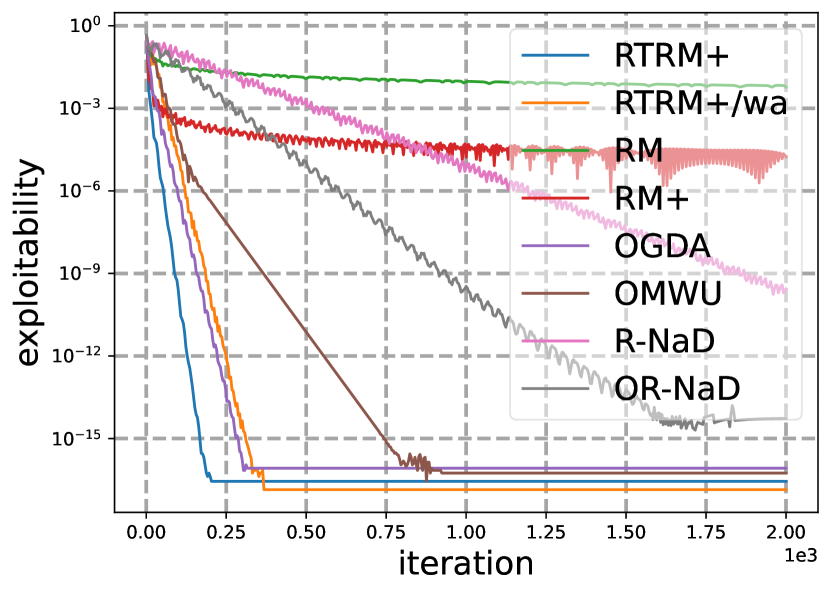
seed 1

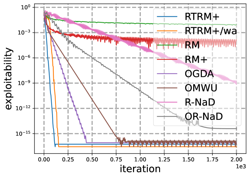
seed 2

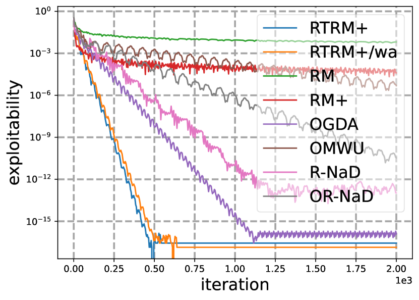
seed 3

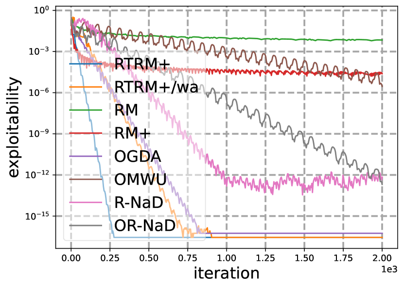
seed 4

seed 5

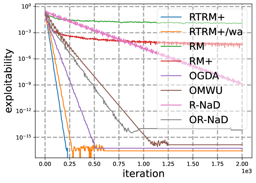
seed 6

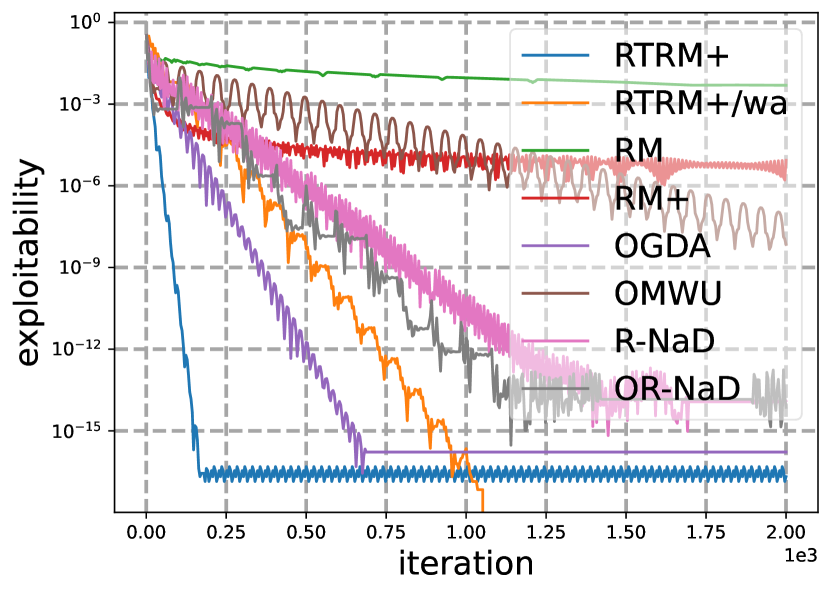
seed 7

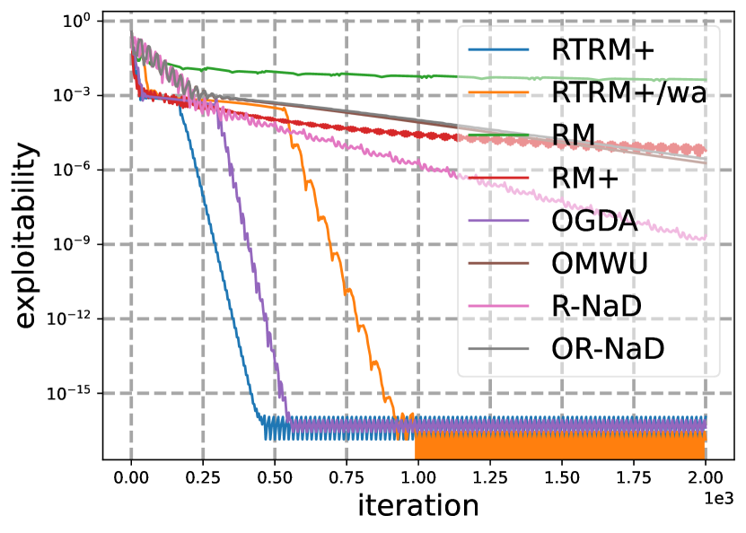
seed 8

seed 9

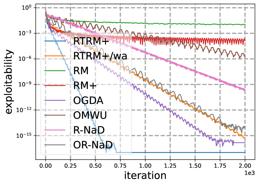
seed 10

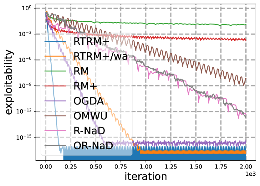
seed 11

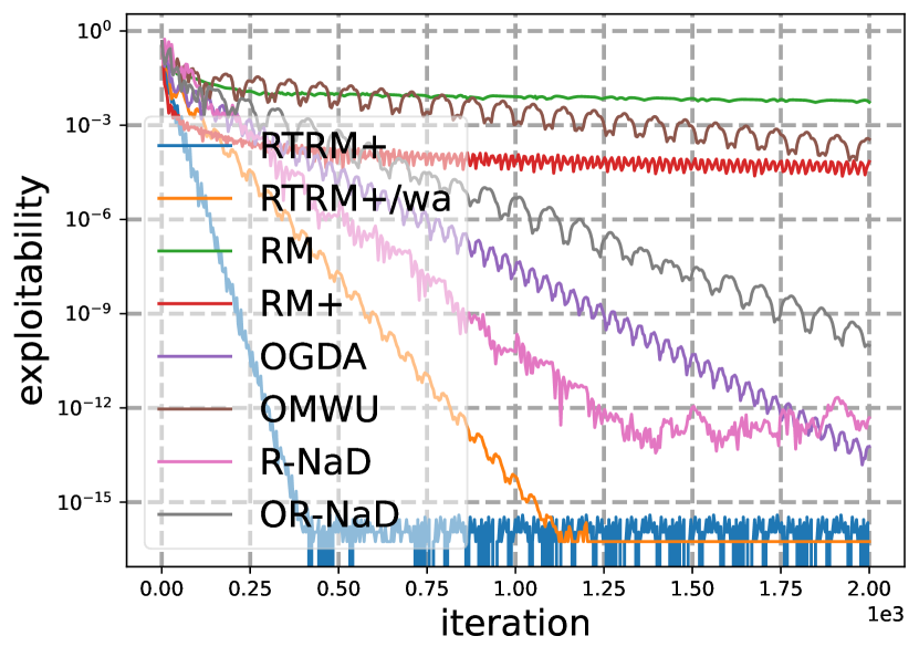
seed 12

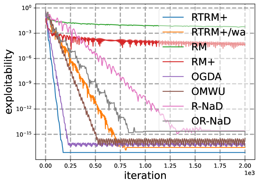
seed 13

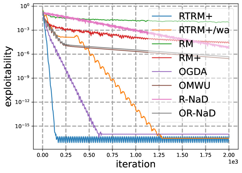
seed 14

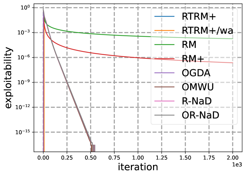
seed 15

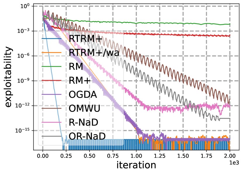
seed 16

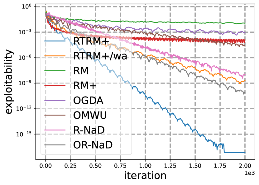
seed 17

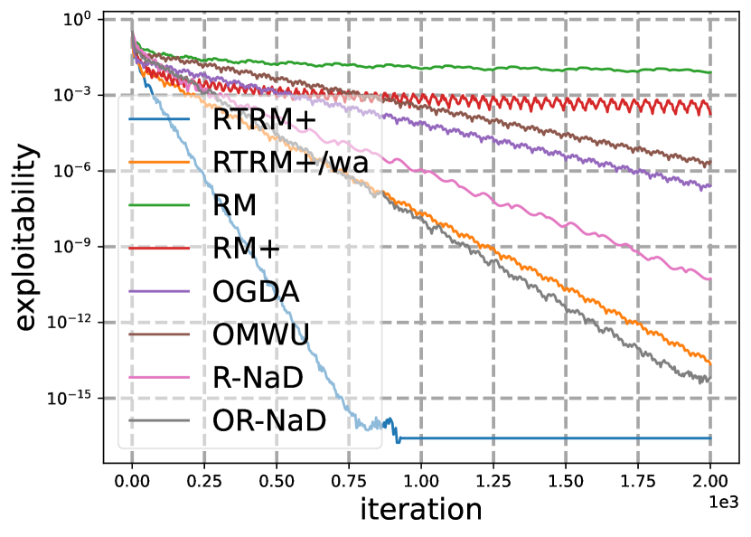
seed 18

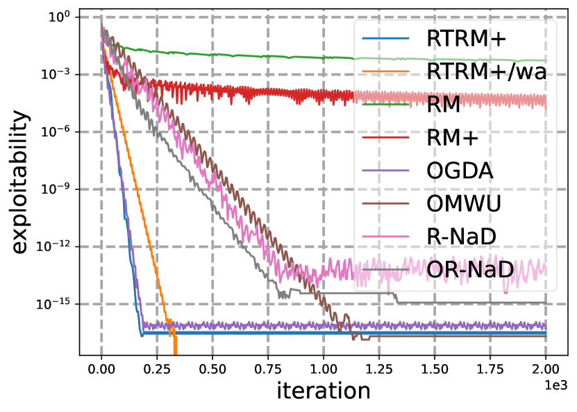
seed 19

Figure 4: Full experimental results in 5x5 normal-form games.

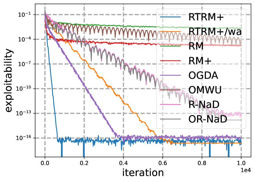
seed 0

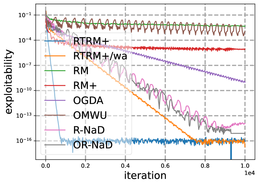
seed 1

seed 2

seed 3

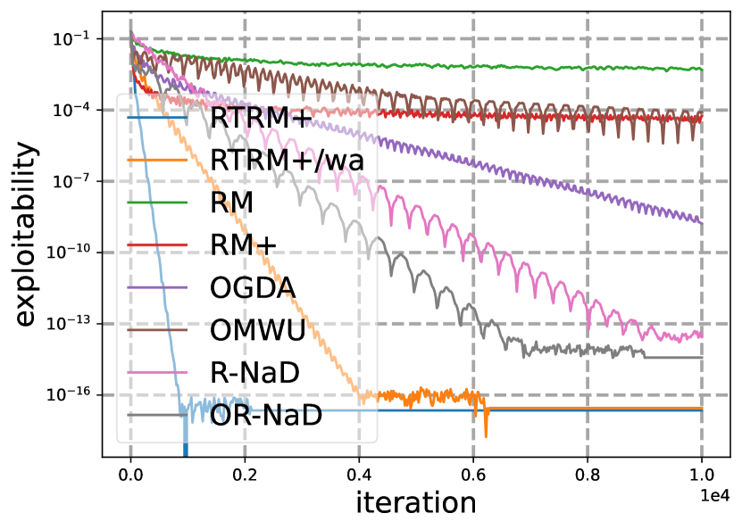
seed 4

seed 5

seed 6

seed 7

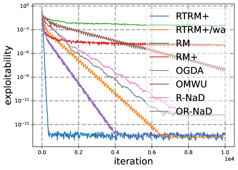
seed 8

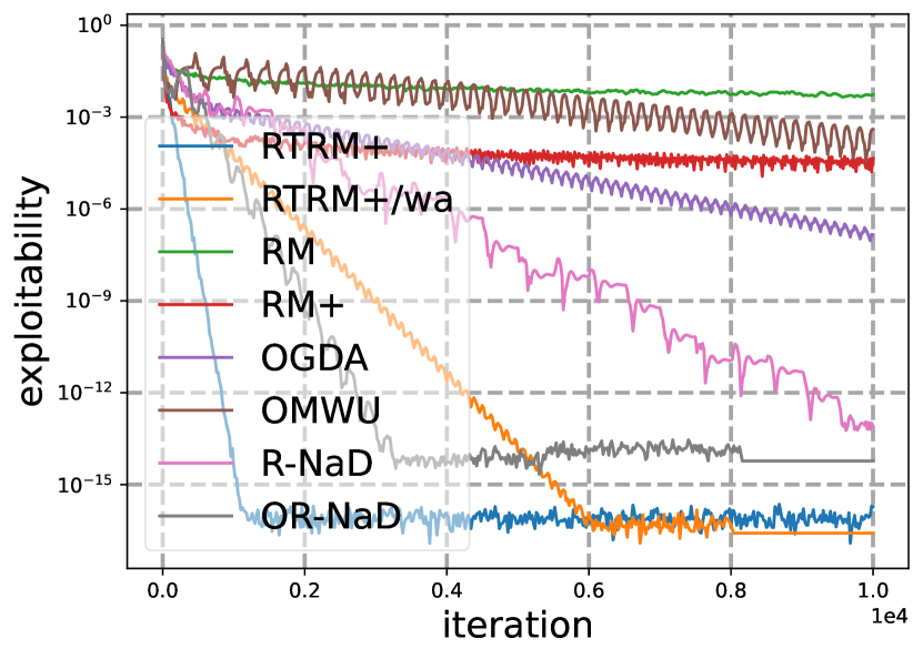
seed 9

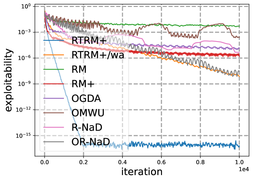
seed 10

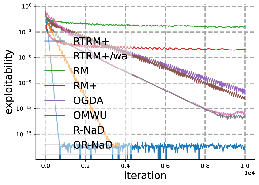
seed 11

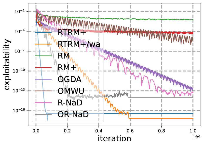
seed 12

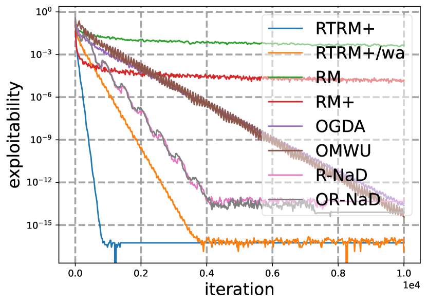
seed 13

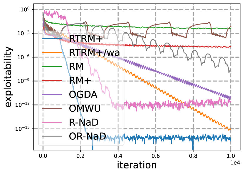
seed 14

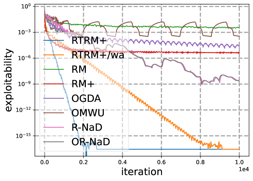
seed 15

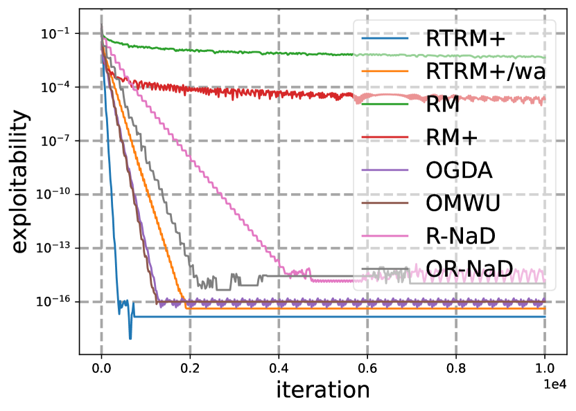
seed 16

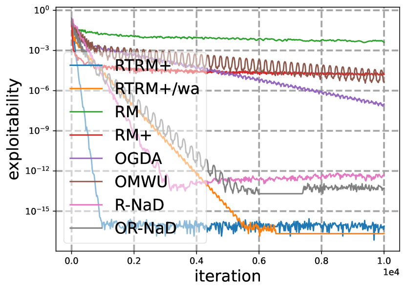
seed 17

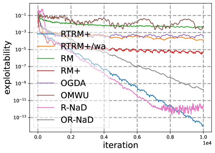
seed 18

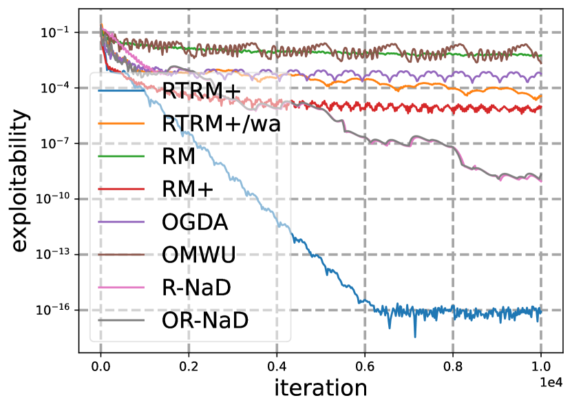
seed 19

Figure 5: Full experimental results in 10x10 normal-form games.

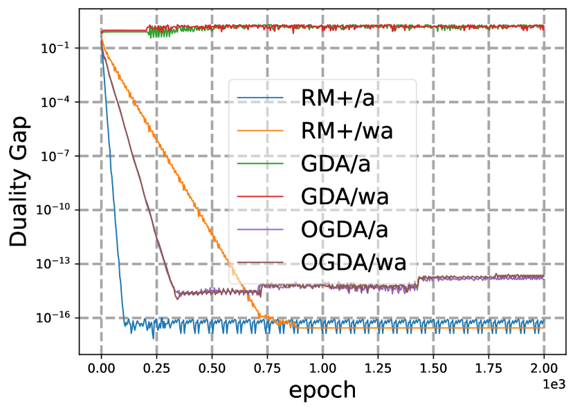
seed 0

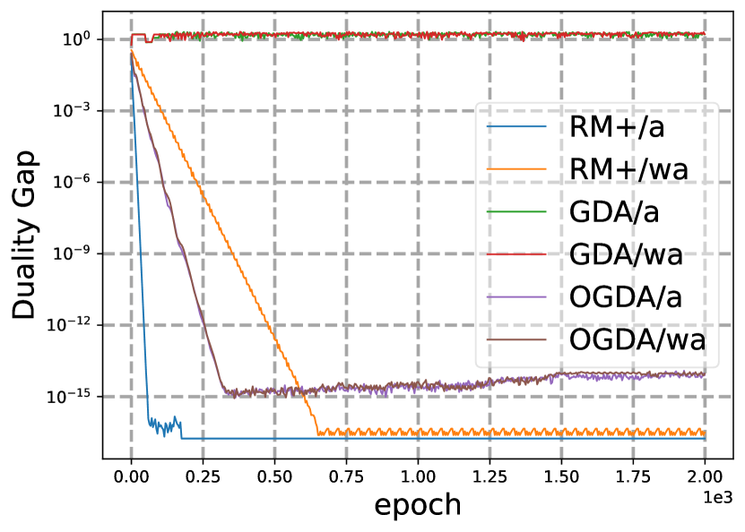
seed 1

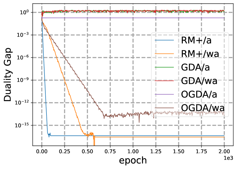
seed 2

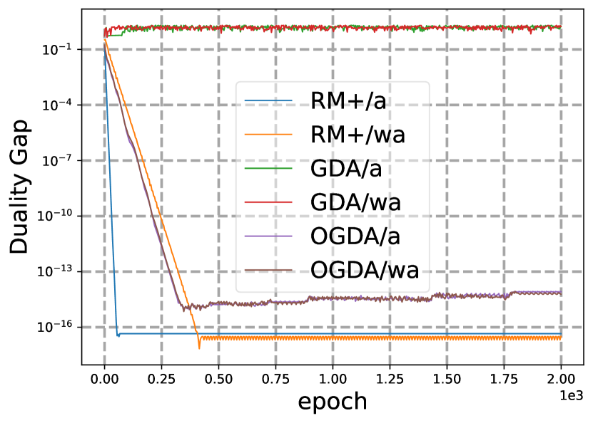
seed 3

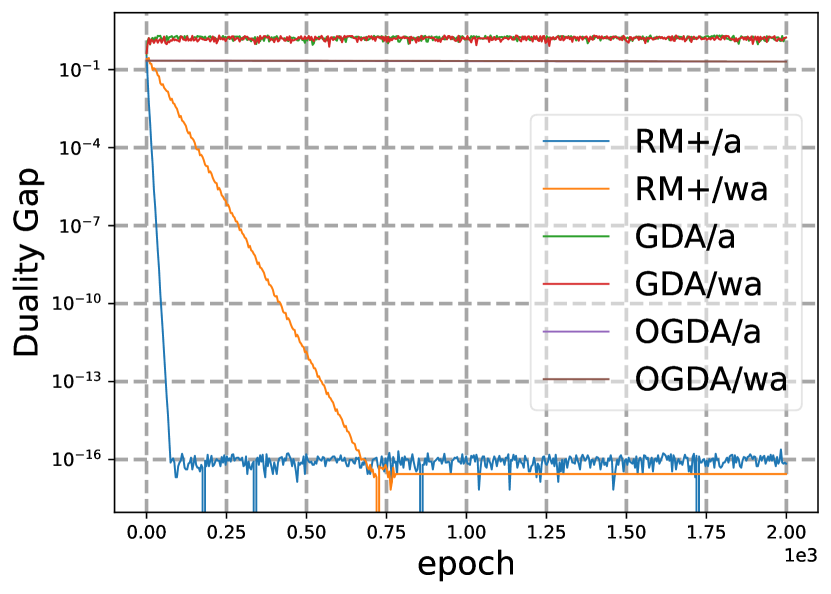
seed 4

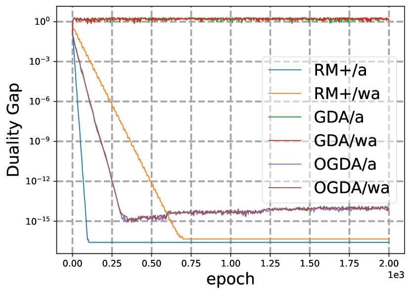
seed 5

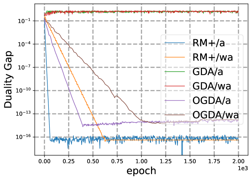
seed 6

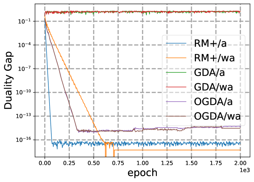
seed 7

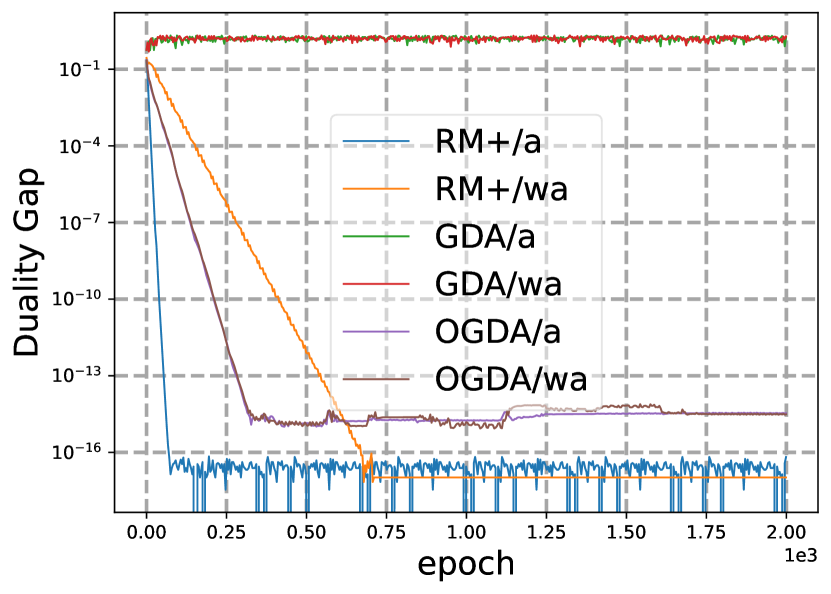
seed 8

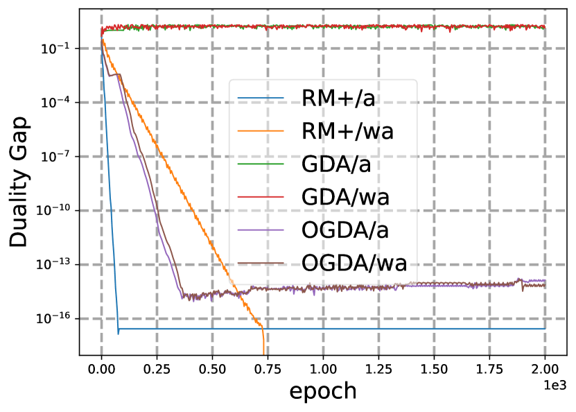
seed 9

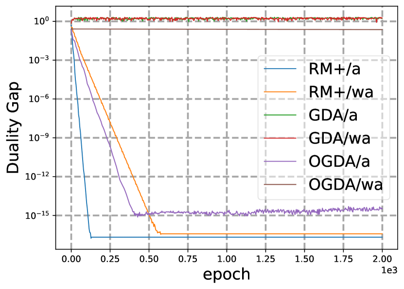
seed 10

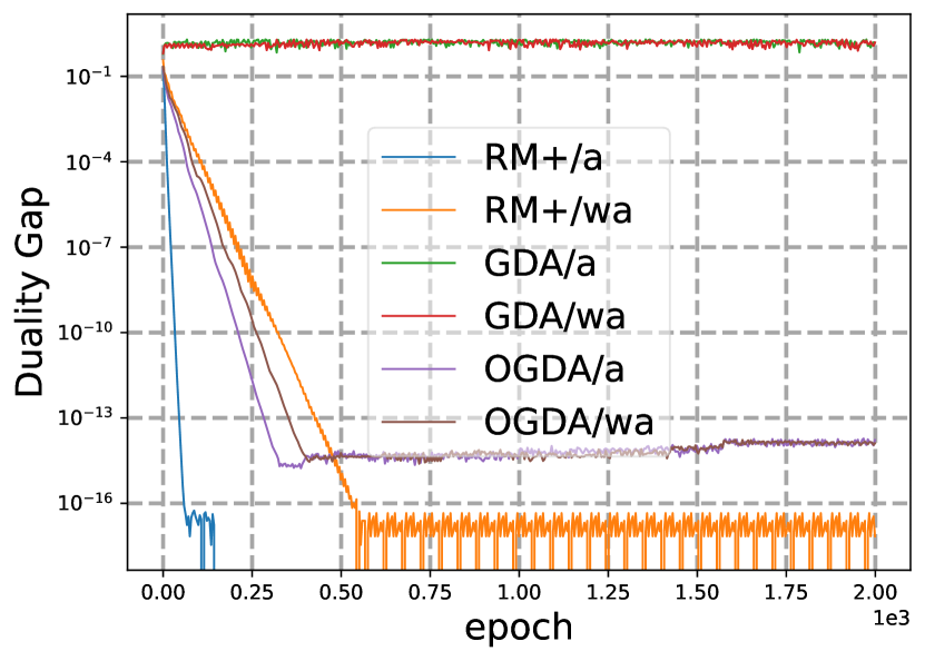
seed 11

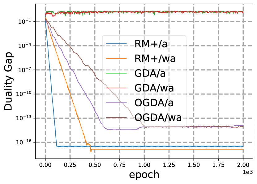
seed 12

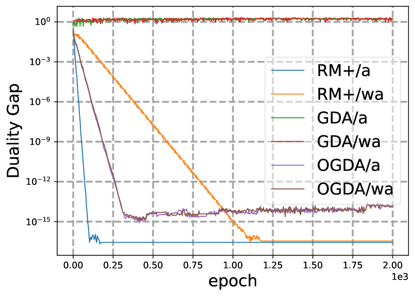
seed 13

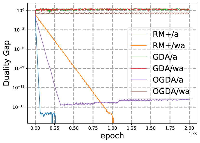
seed 14

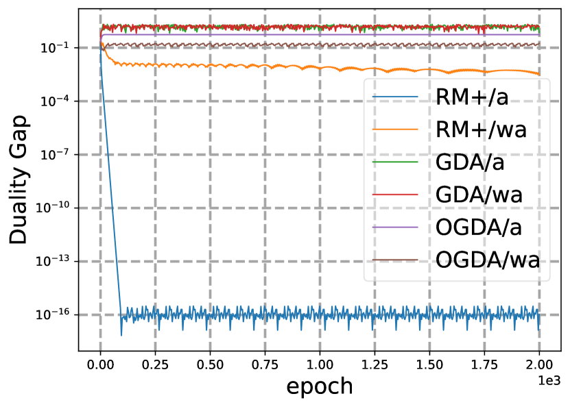
seed 15

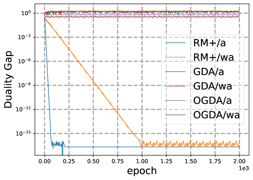
seed 16

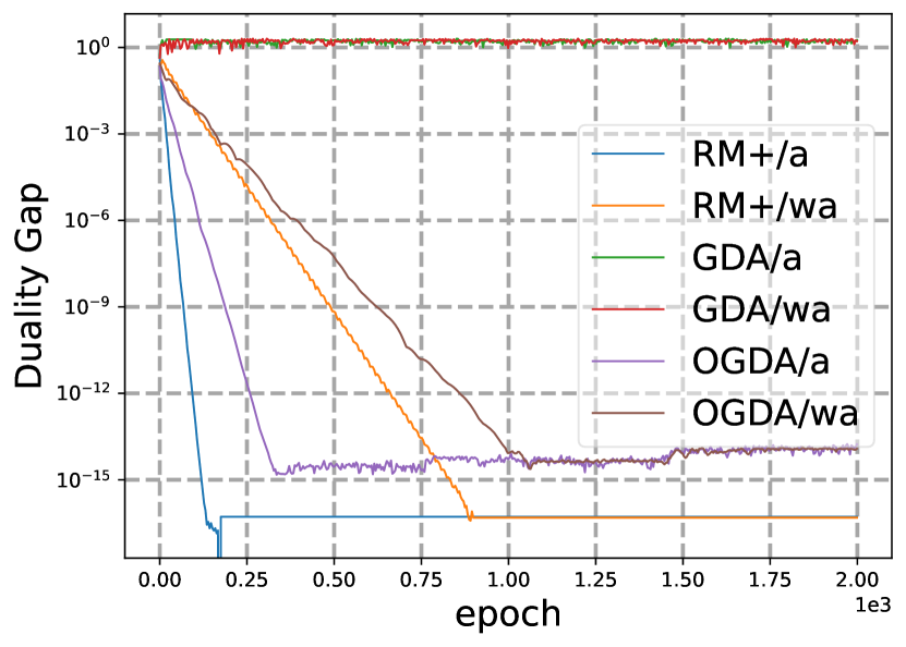
seed 17

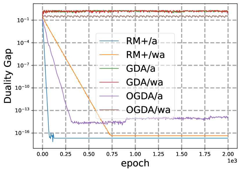
seed 18

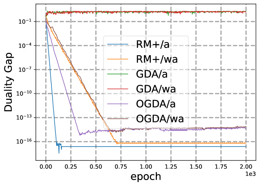
seed 19

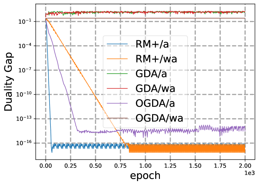
seed 20

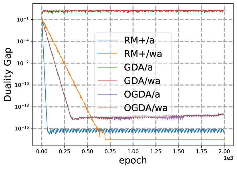
seed 21

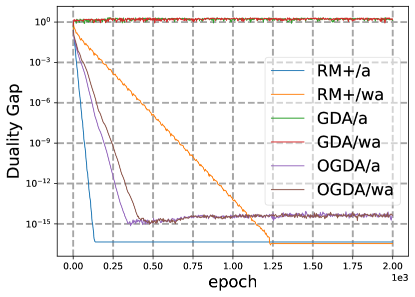
seed 22

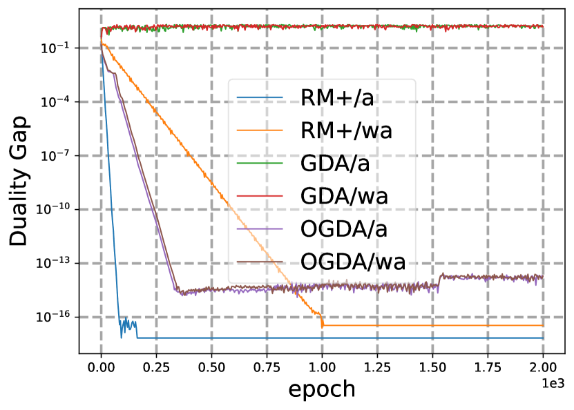
seed 23

Figure 6: Experimental results in strongly convex-concave optimization problems where $\mu=1$ and the additional regularizer is defined in Eq. (6).

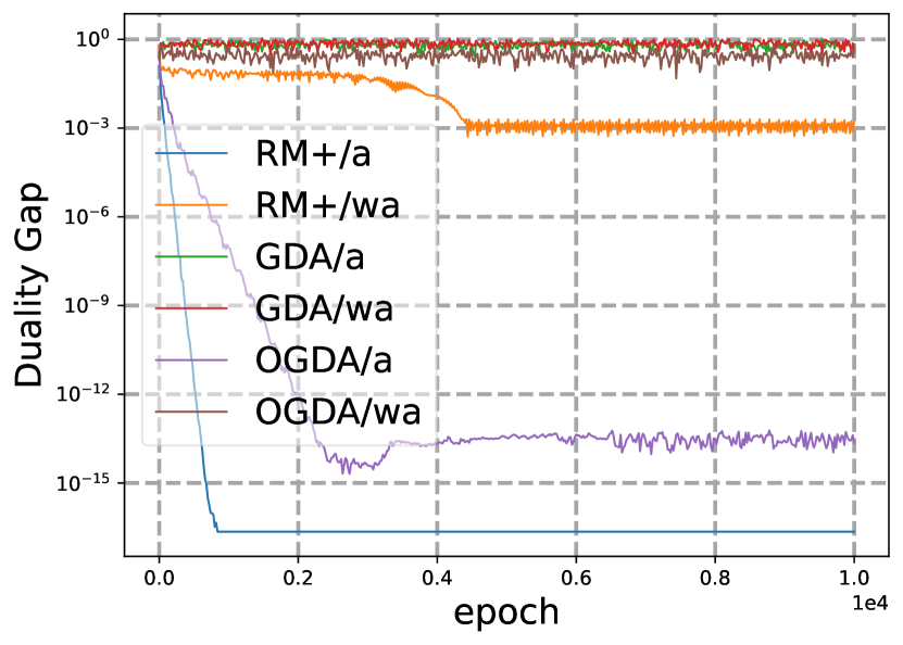
seed 0

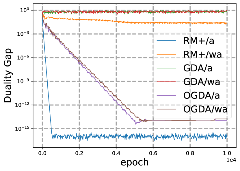
seed 1

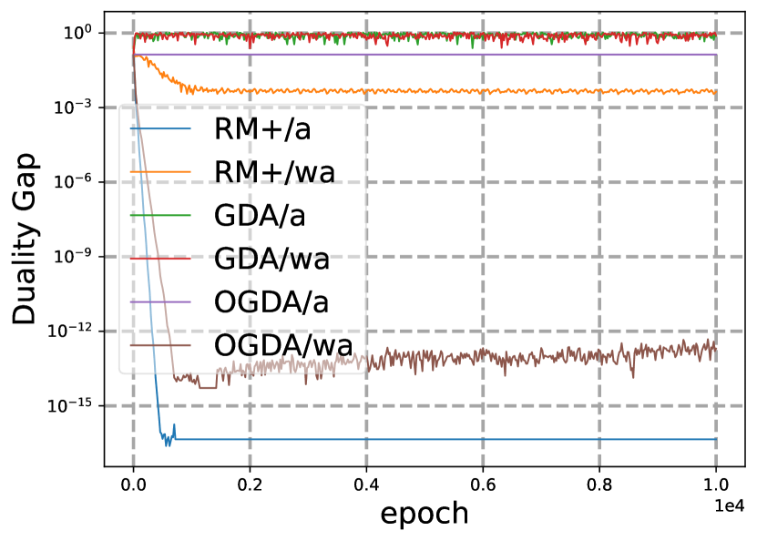
seed 2

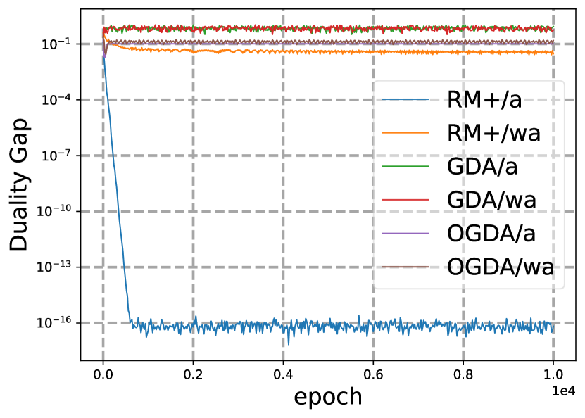
seed 3

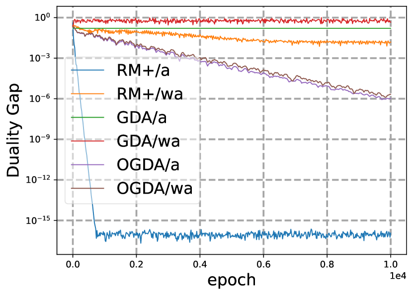
seed 4

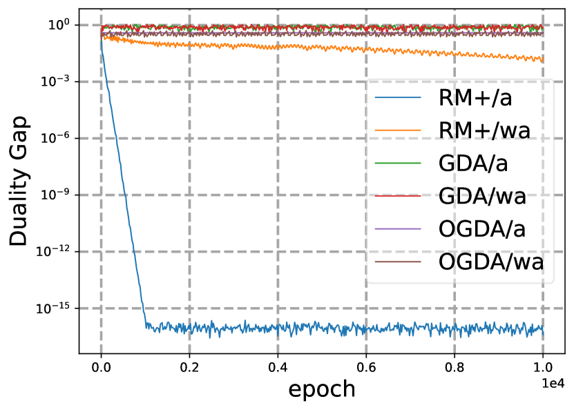
seed 5

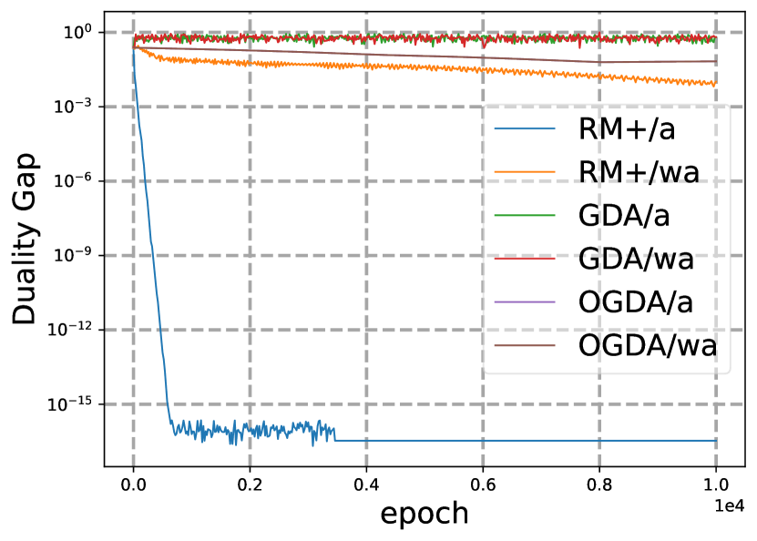
seed 6

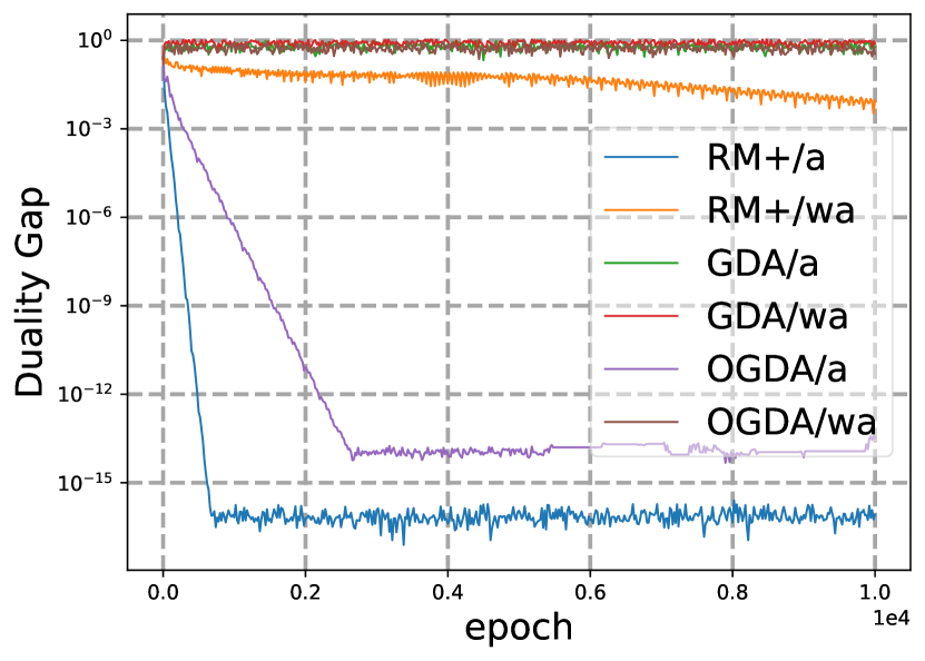
seed 7

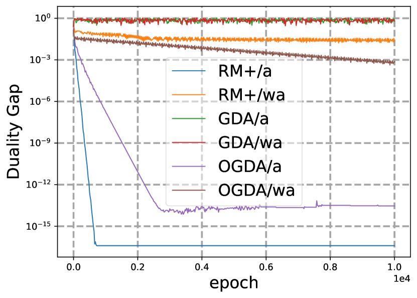
seed 8

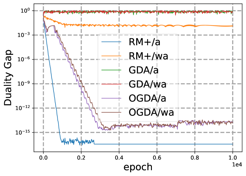
seed 9

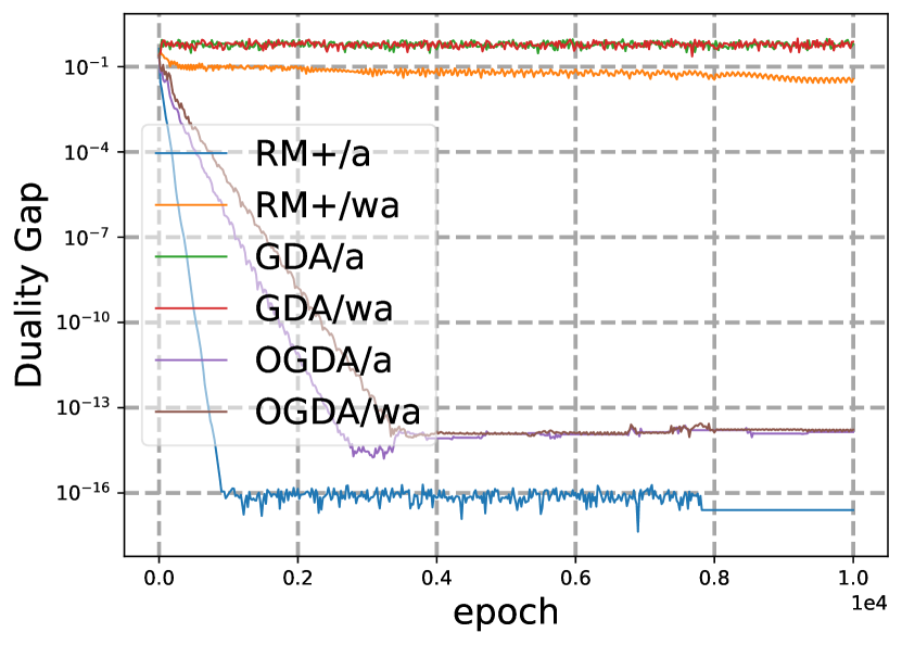
seed 10

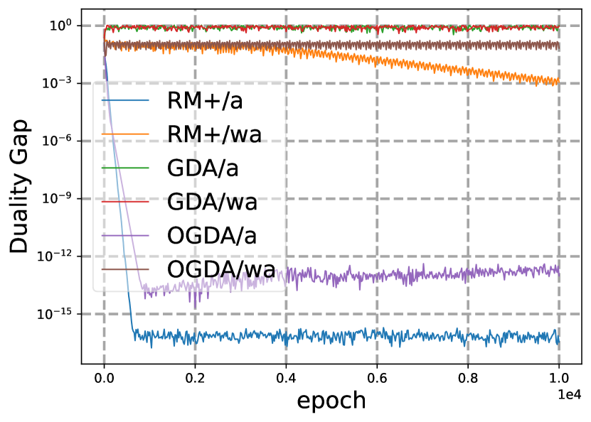
seed 11

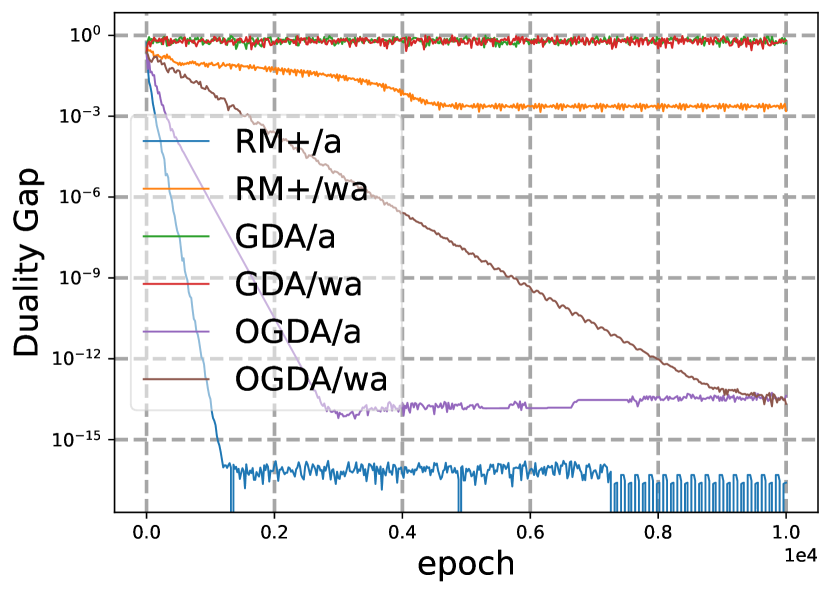
seed 12

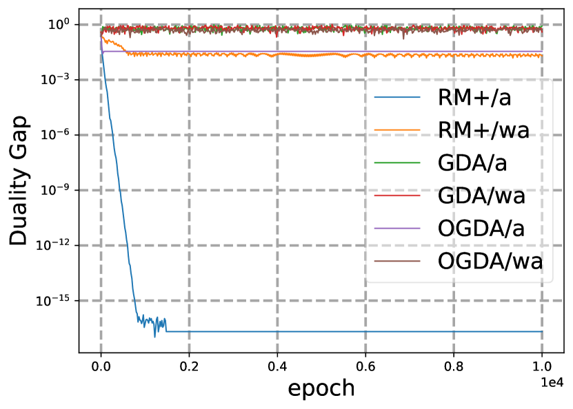
seed 13

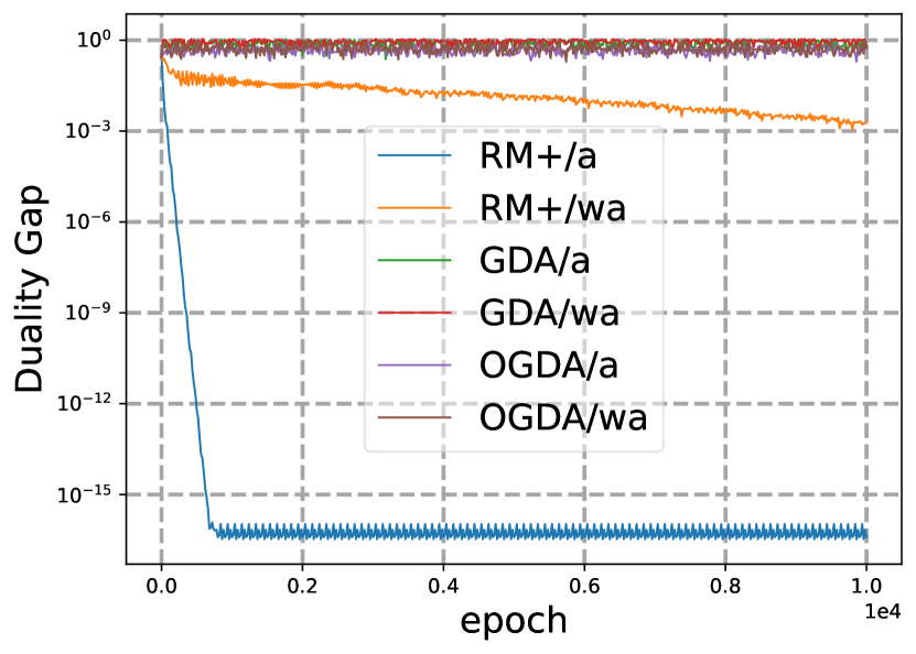
seed 14

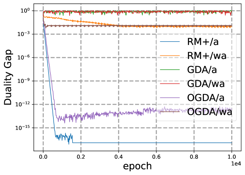
seed 15

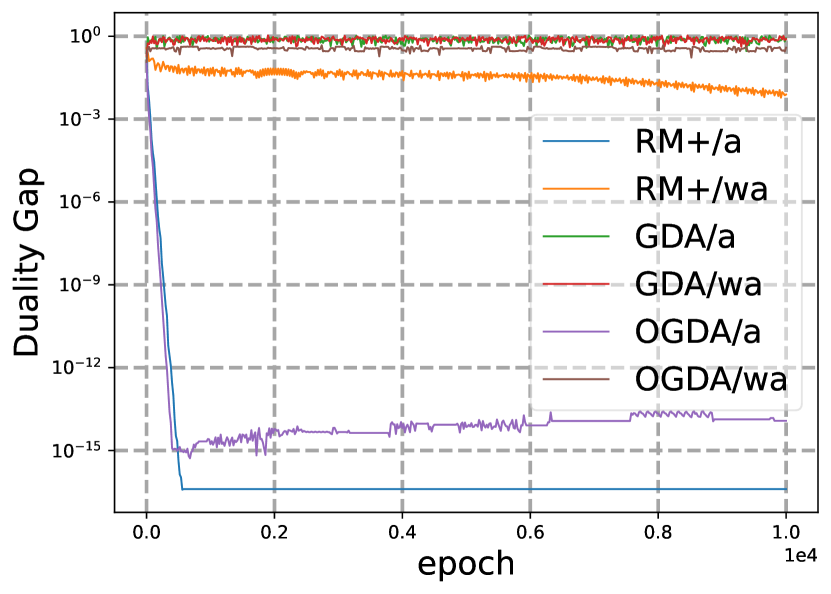
seed 16

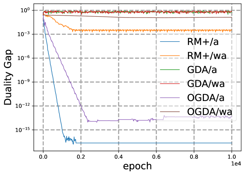
seed 17

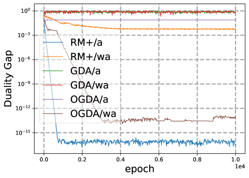
seed 18

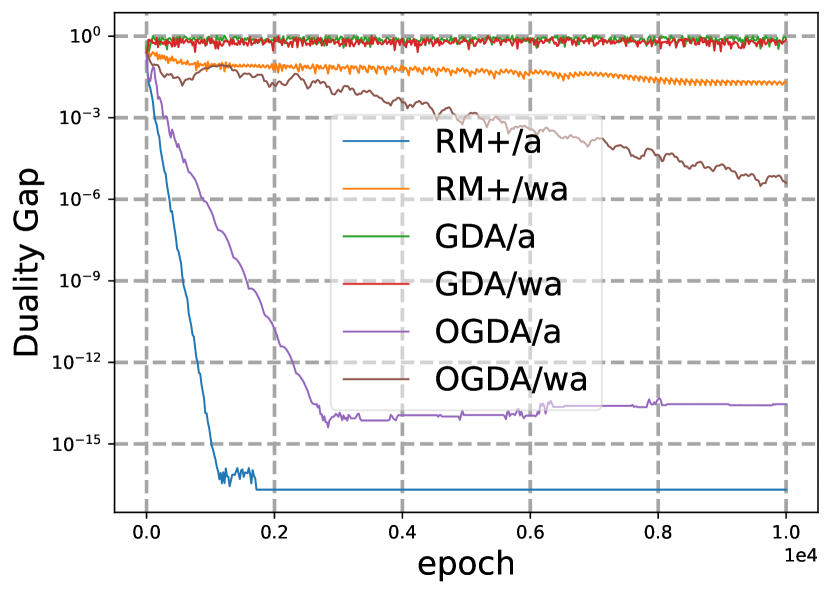
seed 19

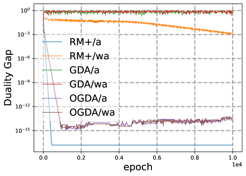
seed 20

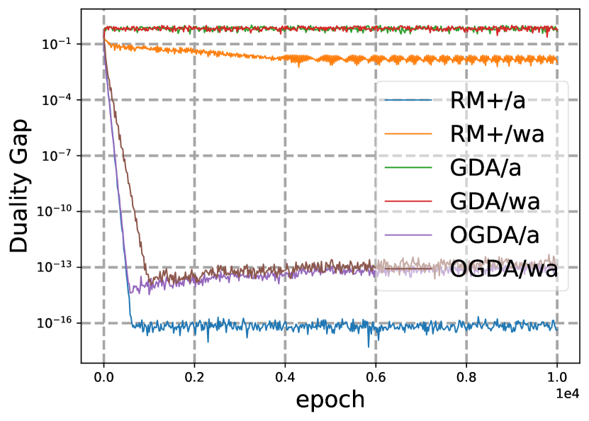
seed 21

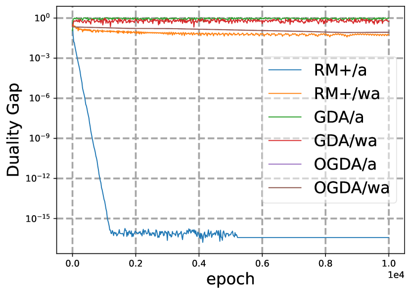
seed 22

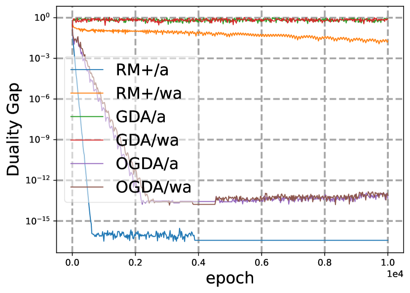
seed 23

Figure 7: Experimental results in strongly convex-concave optimization problems where $\mu=0.1$ and the additional regularizer is defined in Eq. (6).

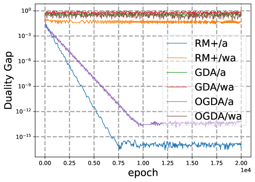
seed 0

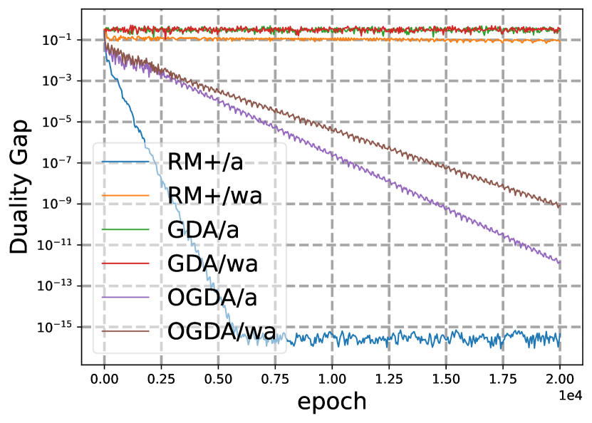
seed 1

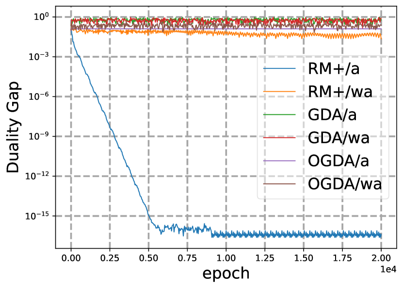
seed 2

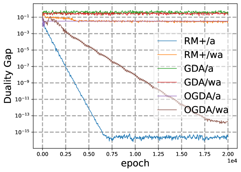
seed 3

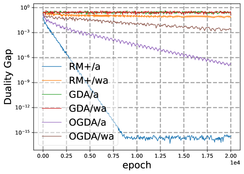
seed 4

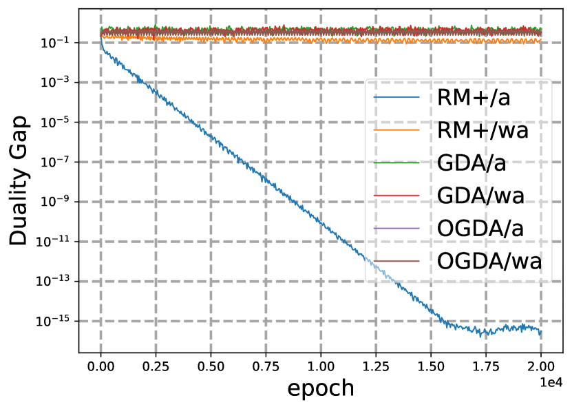
seed 5

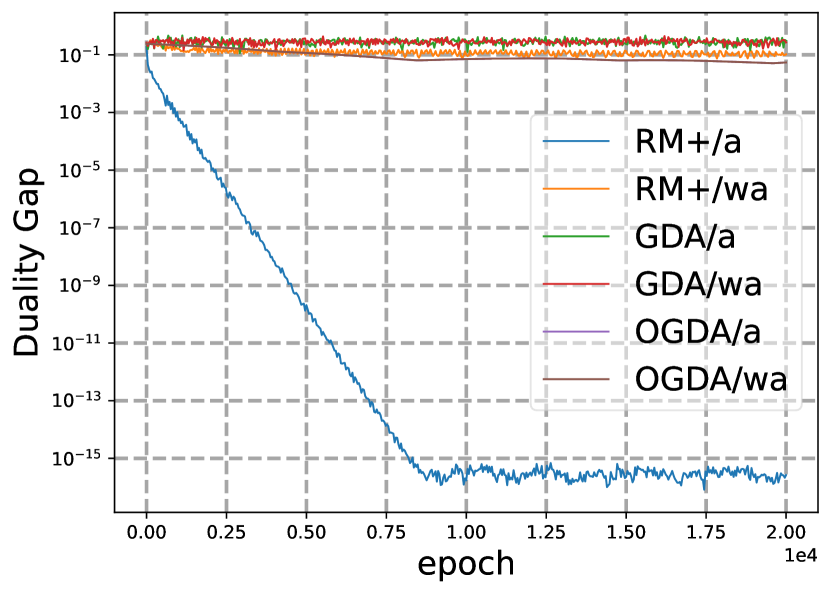
seed 6

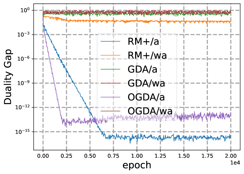
seed 7

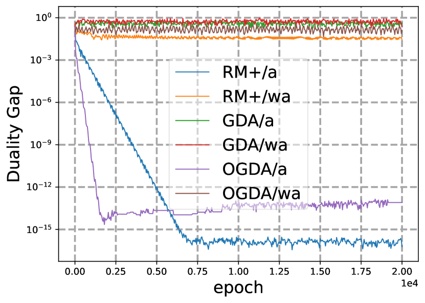
seed 8

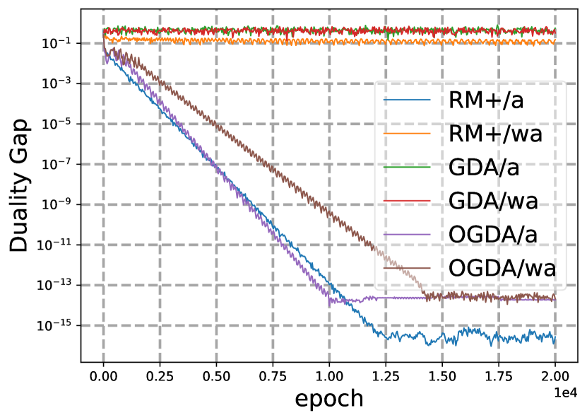
seed 9

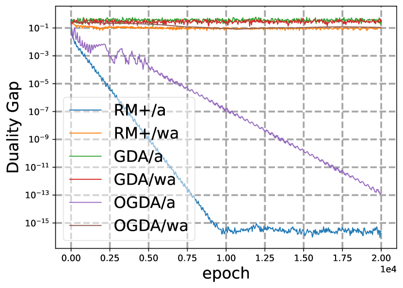
seed 10

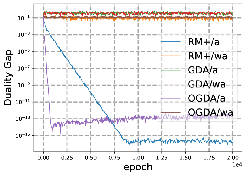
seed 11

seed 12

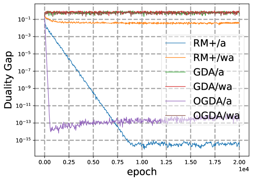
seed 13

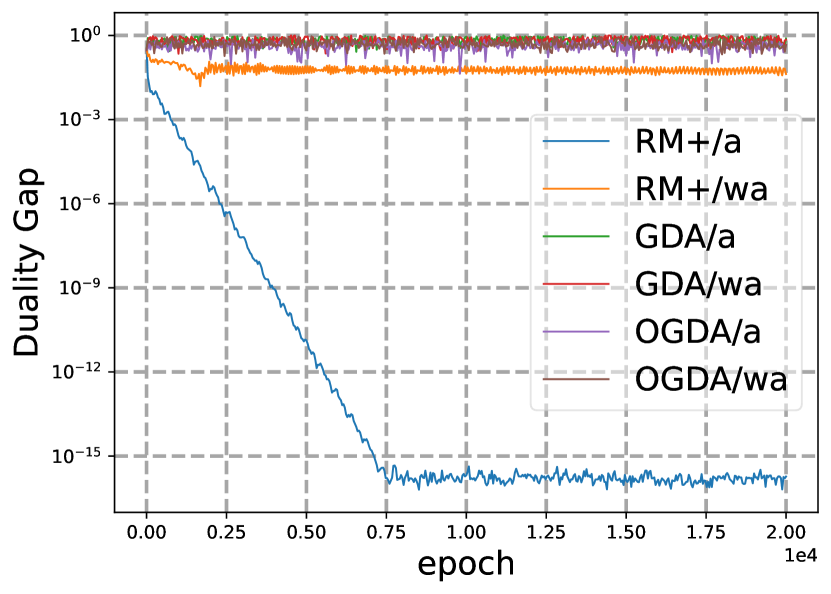
seed 14

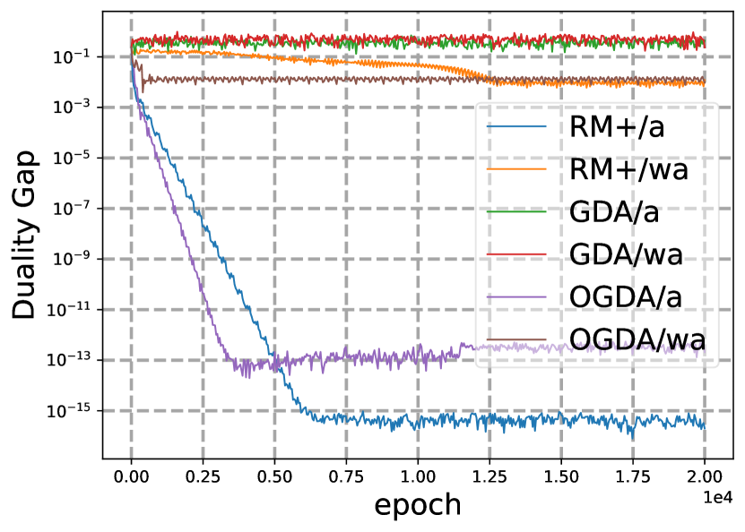
seed 15

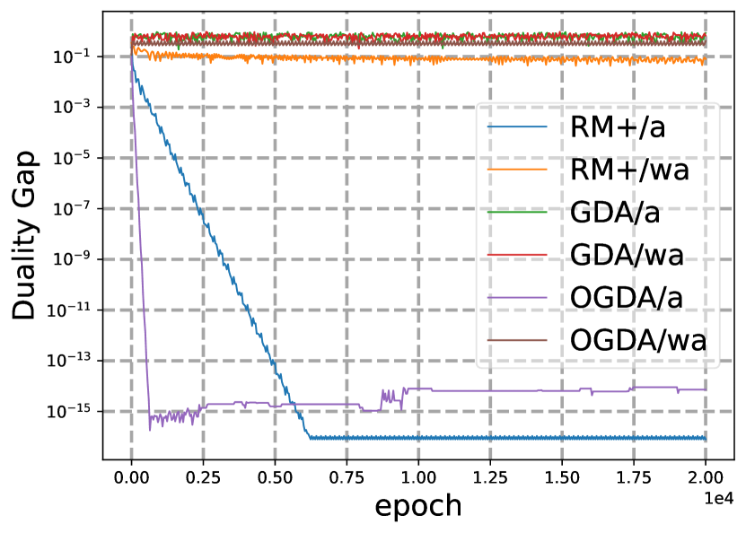
seed 16

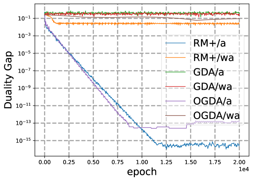
seed 17

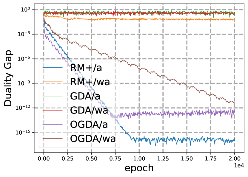
seed 18

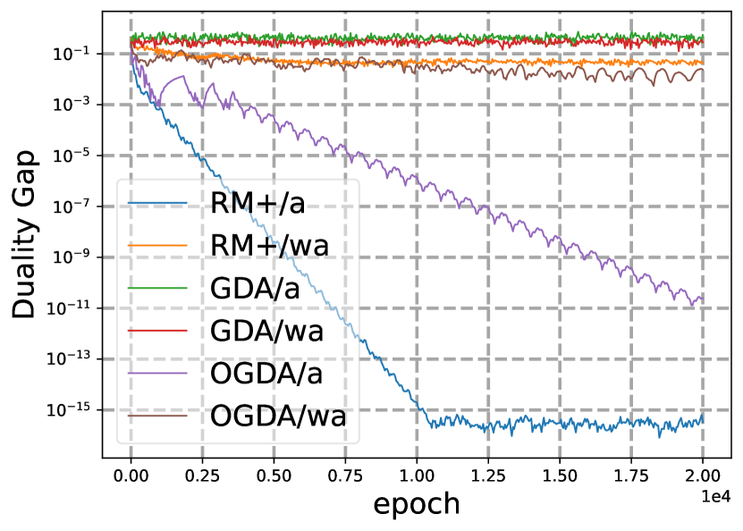
seed 19

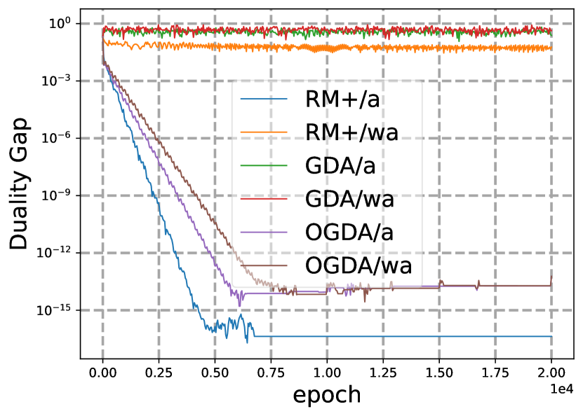
seed 20

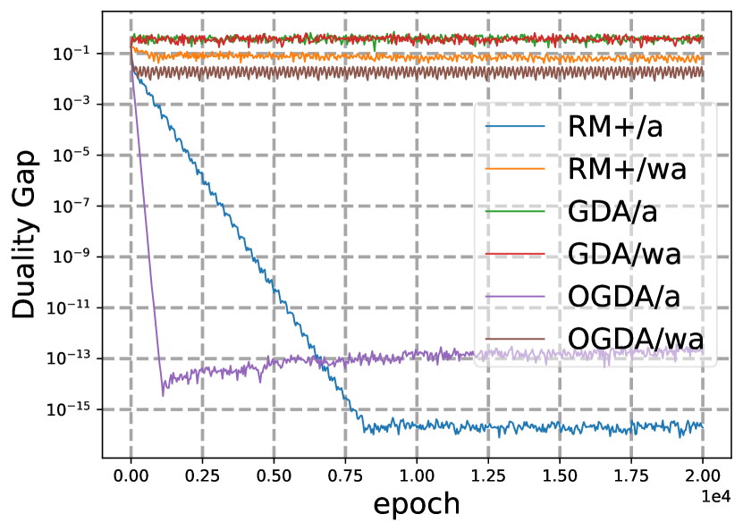
seed 21

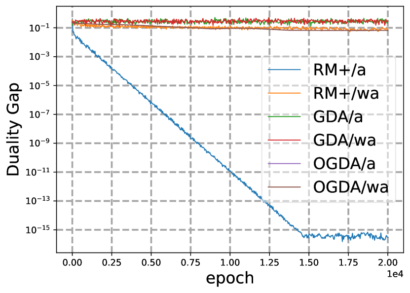
seed 22

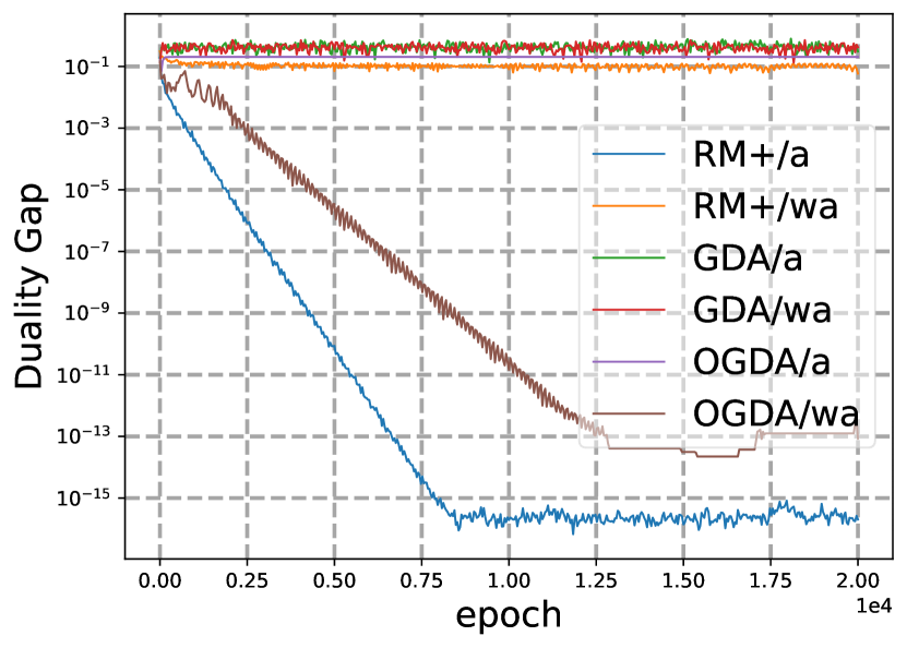
seed 23

Figure 8: Experimental results in strongly convex-concave optimization problems where $\mu=0.01$ and the additional regularizer is defined in Eq. (6).

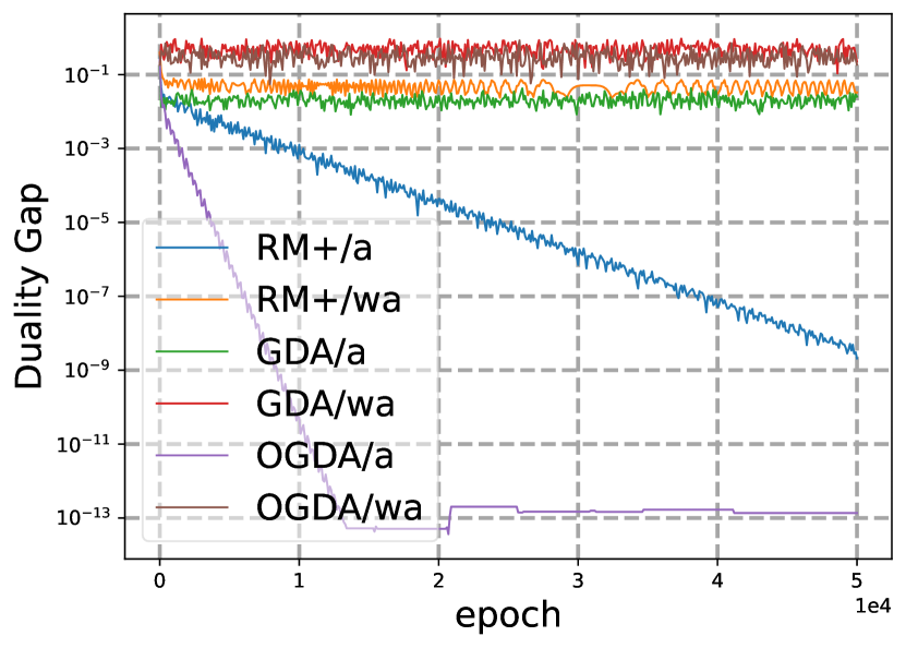
seed 0

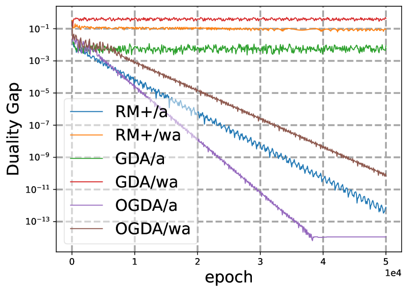
seed 1

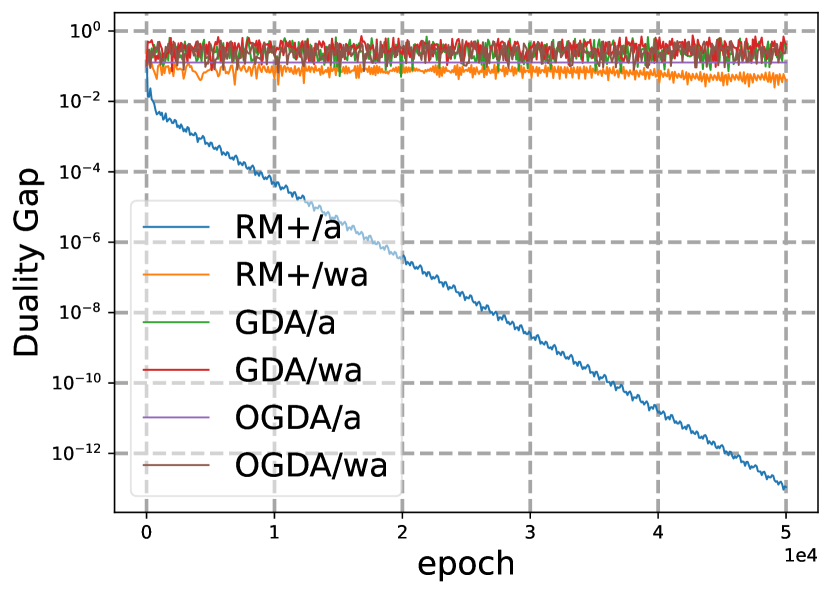
seed 2

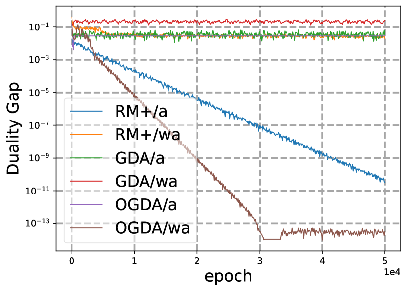
seed 3

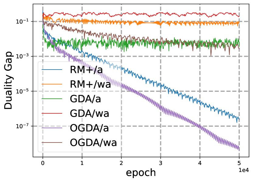
seed 4

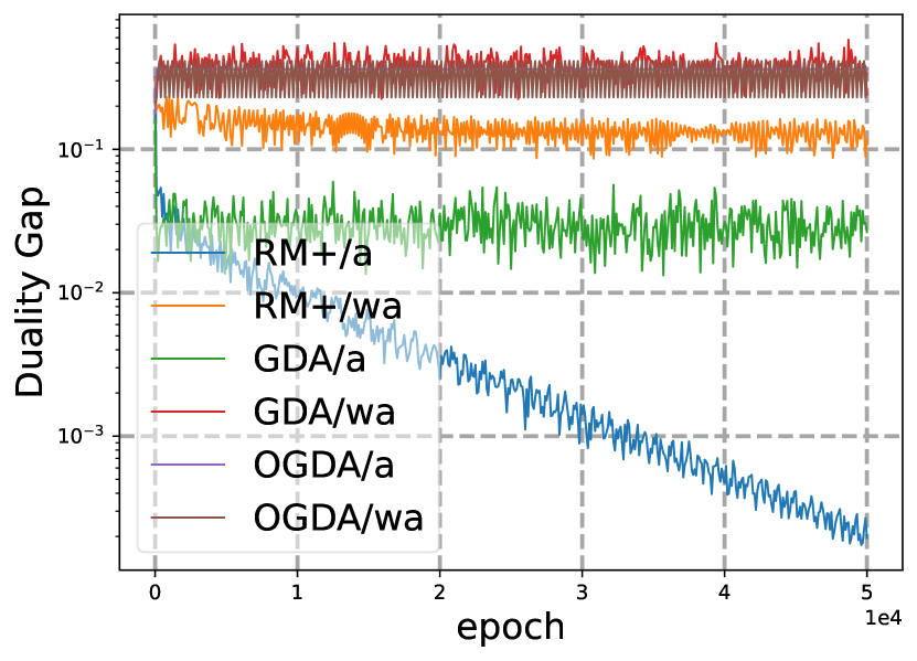
seed 5

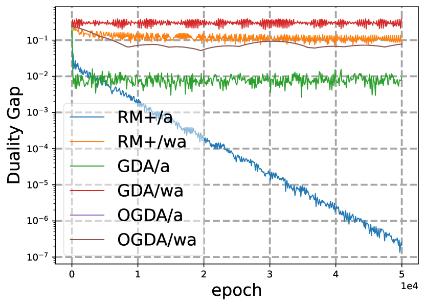
seed 6

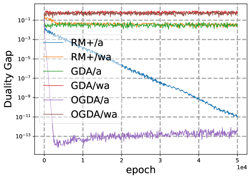
seed 7

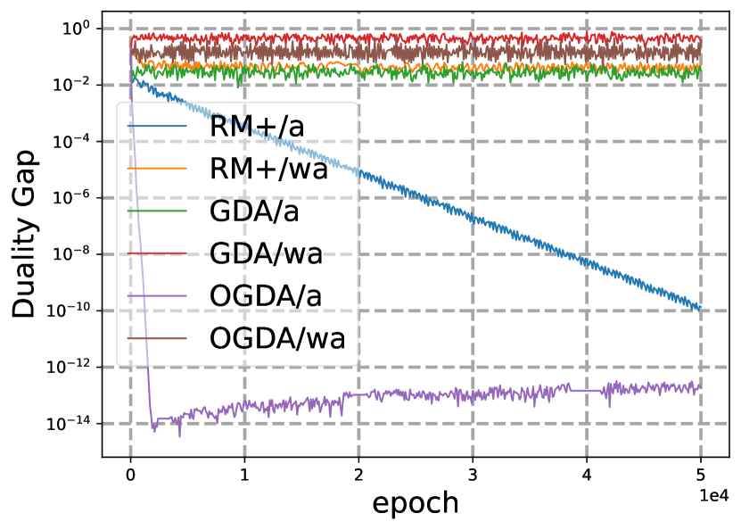
seed 8

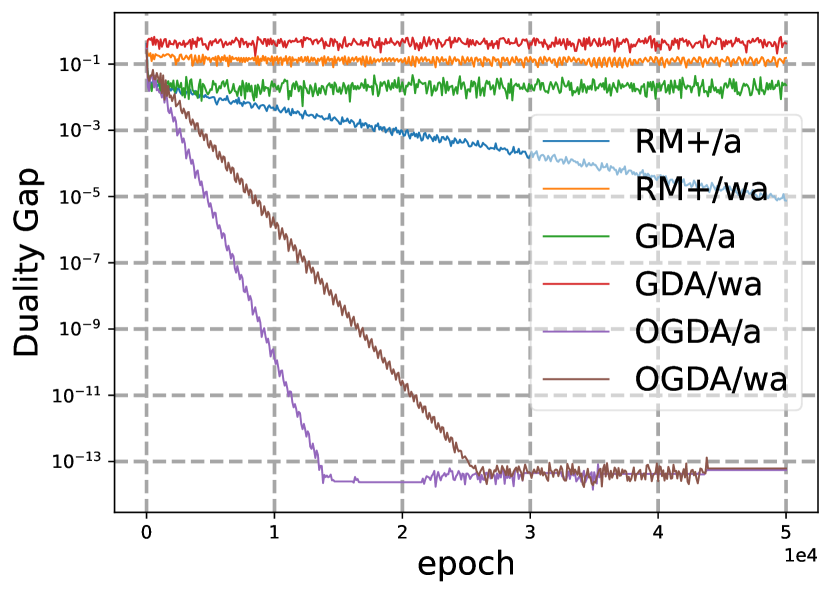
seed 9

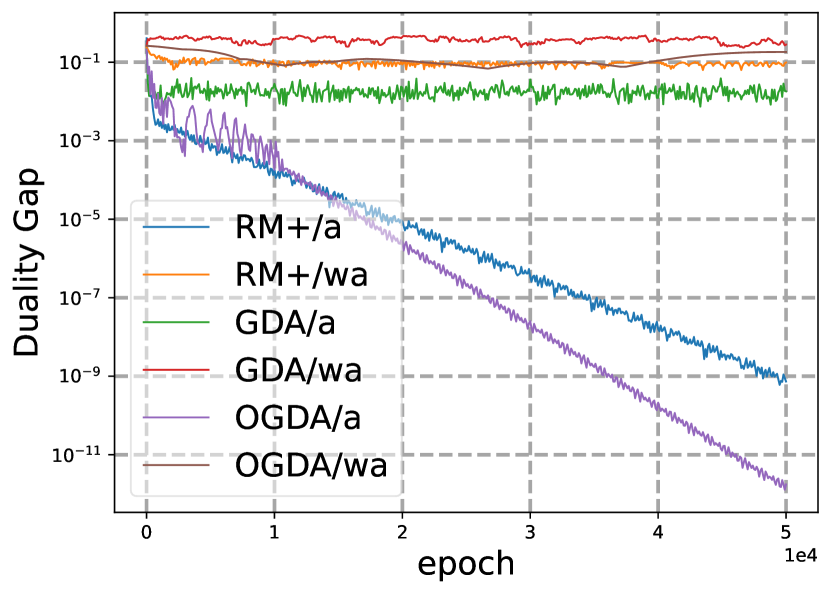
seed 10

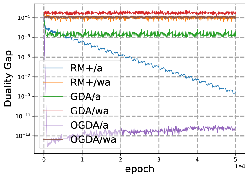
seed 11

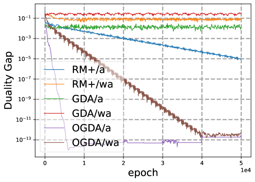
seed 12

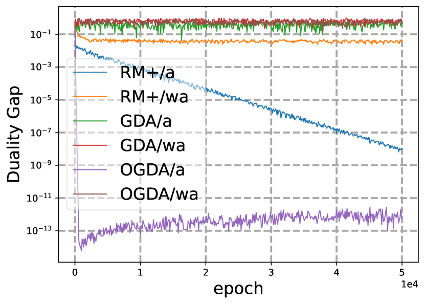
seed 13

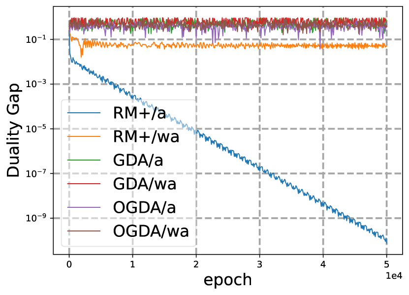
seed 14

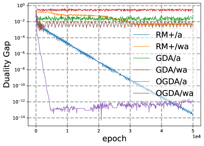
seed 15

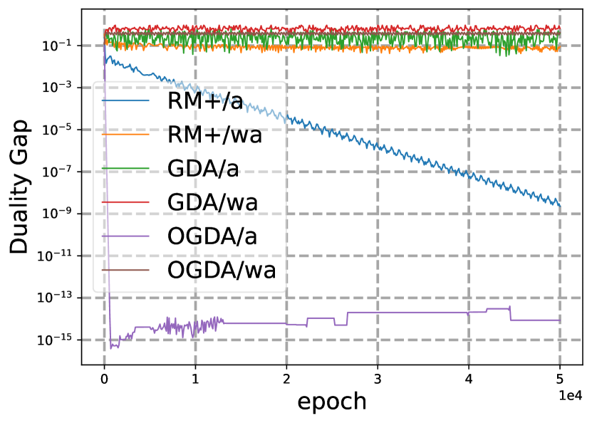
seed 16

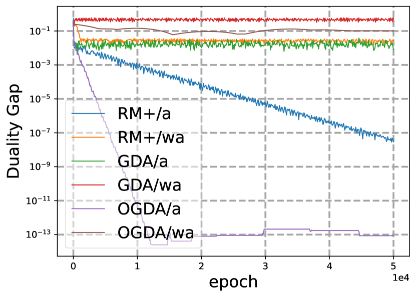
seed 17

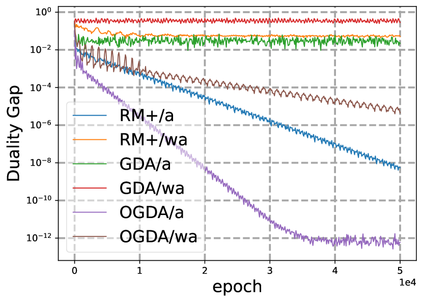
seed 18

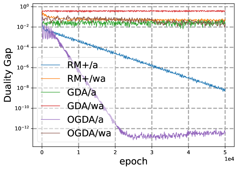
seed 19

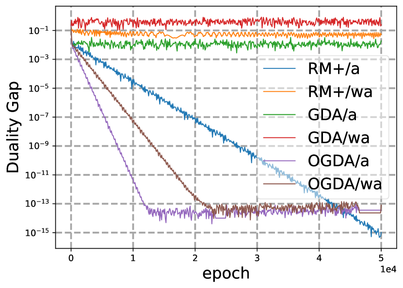
seed 20

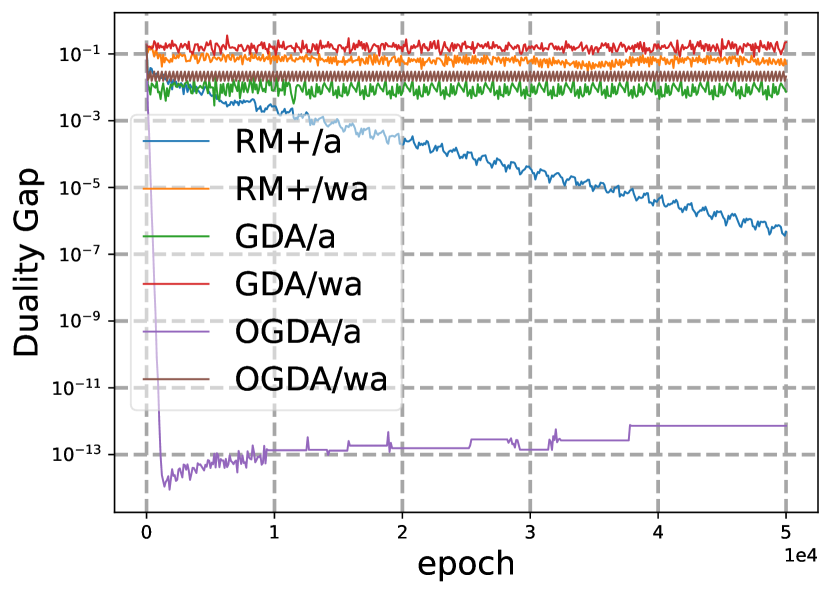
seed 21

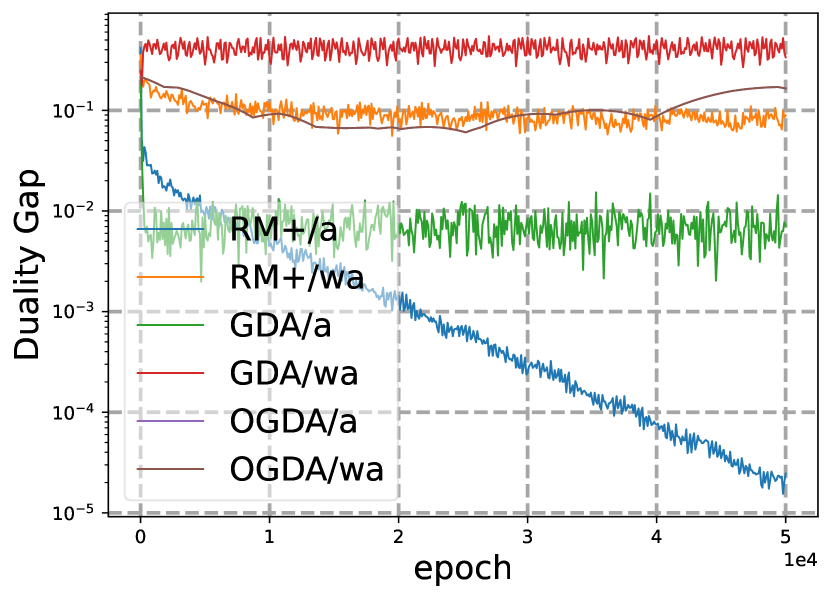
seed 22

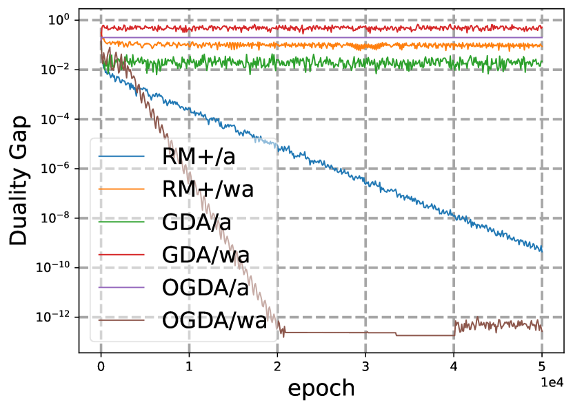
seed 23

Figure 9: Experimental results in strongly convex-concave optimization problems where $\mu=0.001$ and the additional regularizer is defined in Eq. (6).

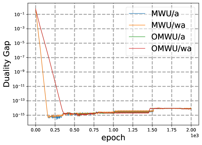
seed 0

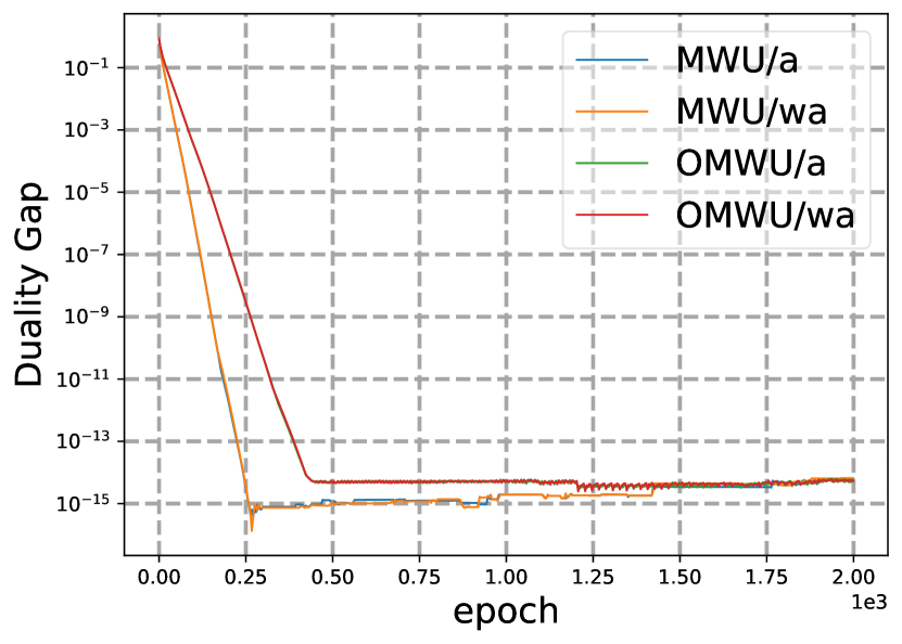
seed 1

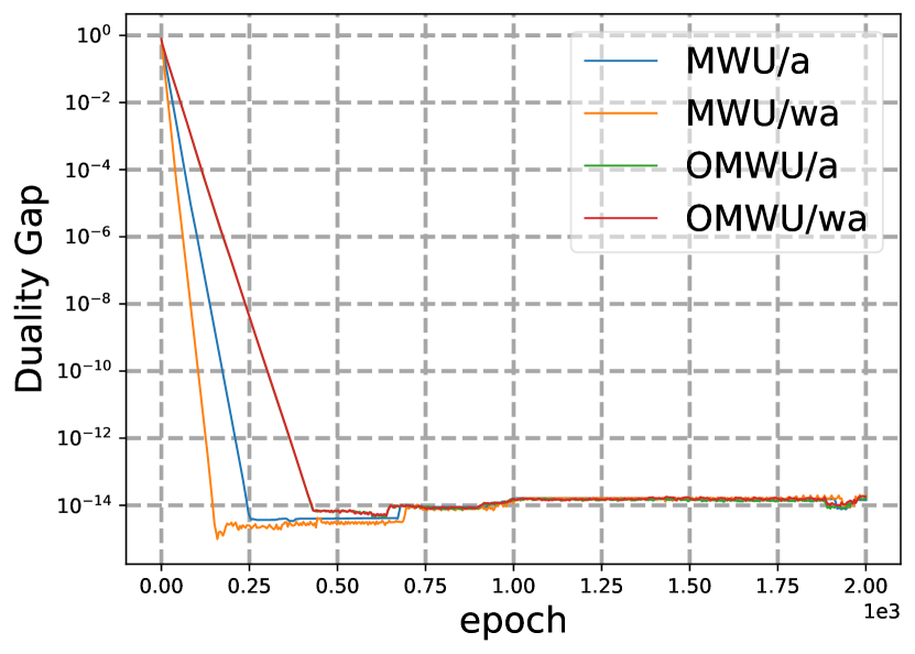
seed 2

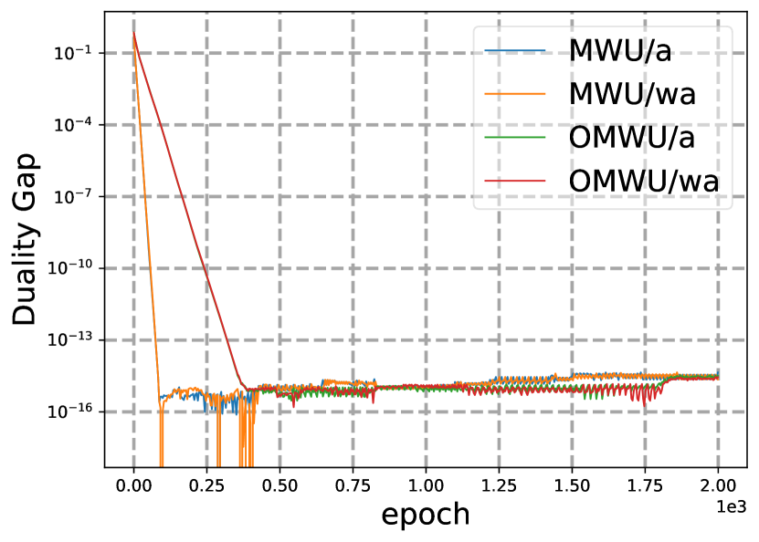
seed 3

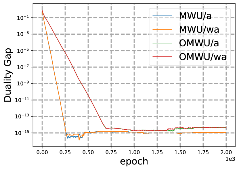
seed 4

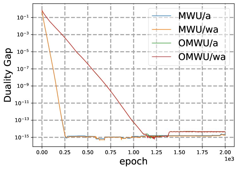
seed 5

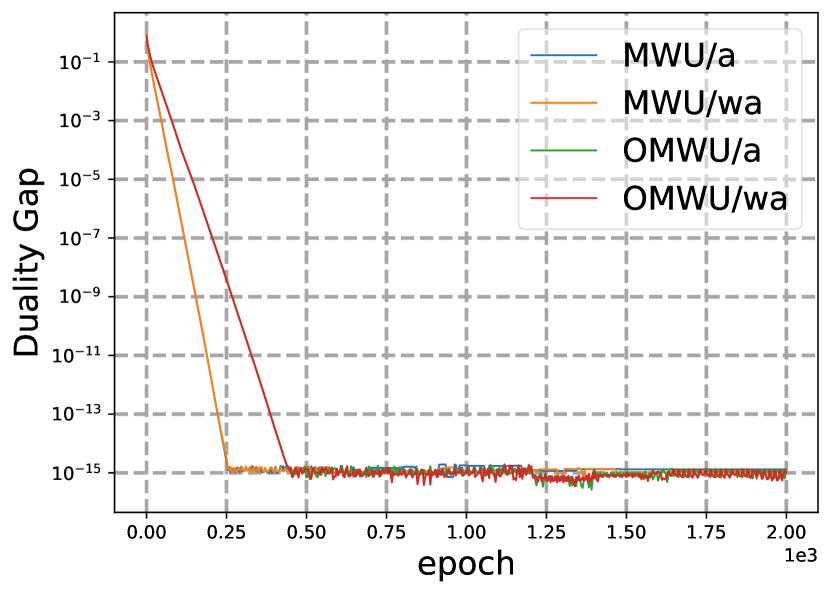
seed 6

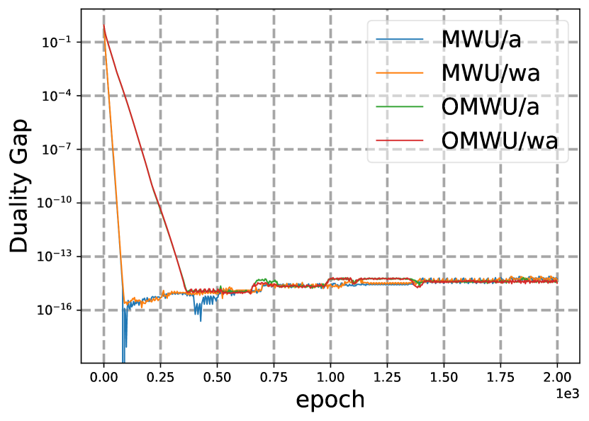
seed 7

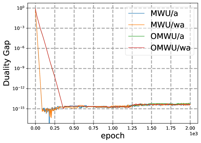
seed 8

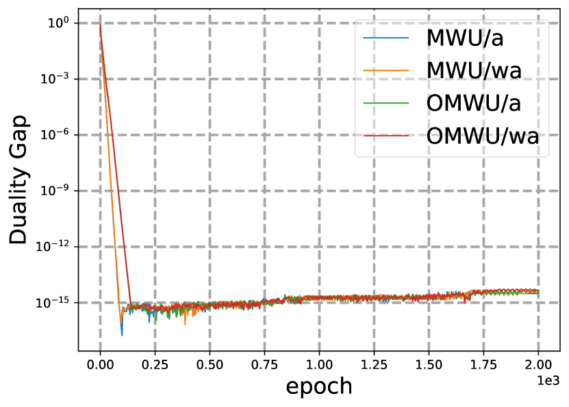
seed 9

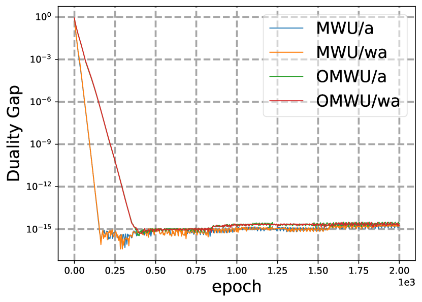
seed 10

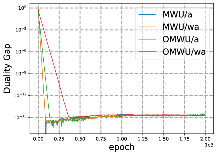
seed 11

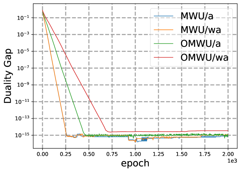
seed 12

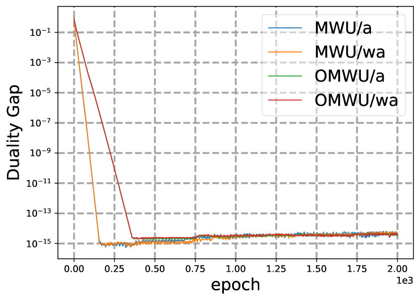
seed 13

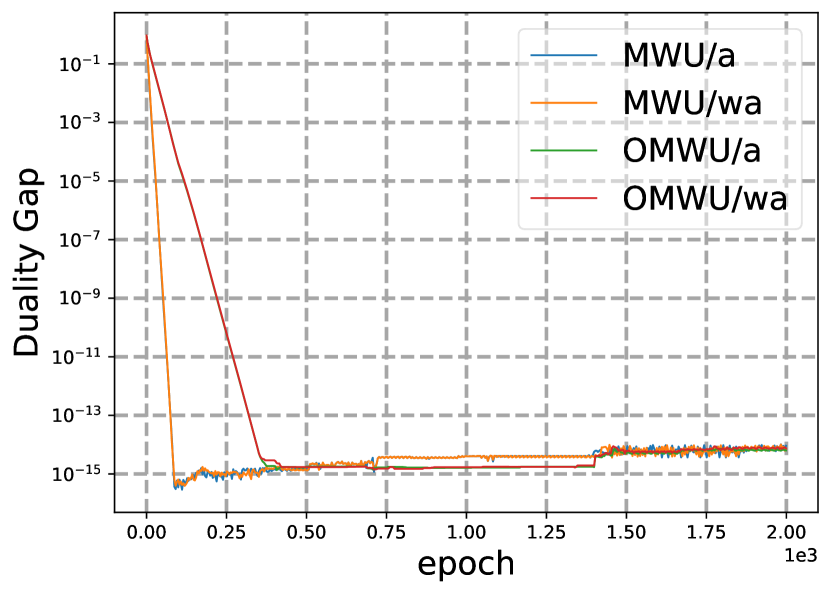
seed 14

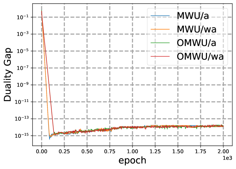
seed 15

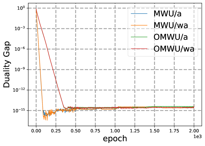
seed 16

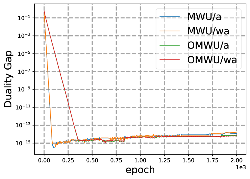
seed 17

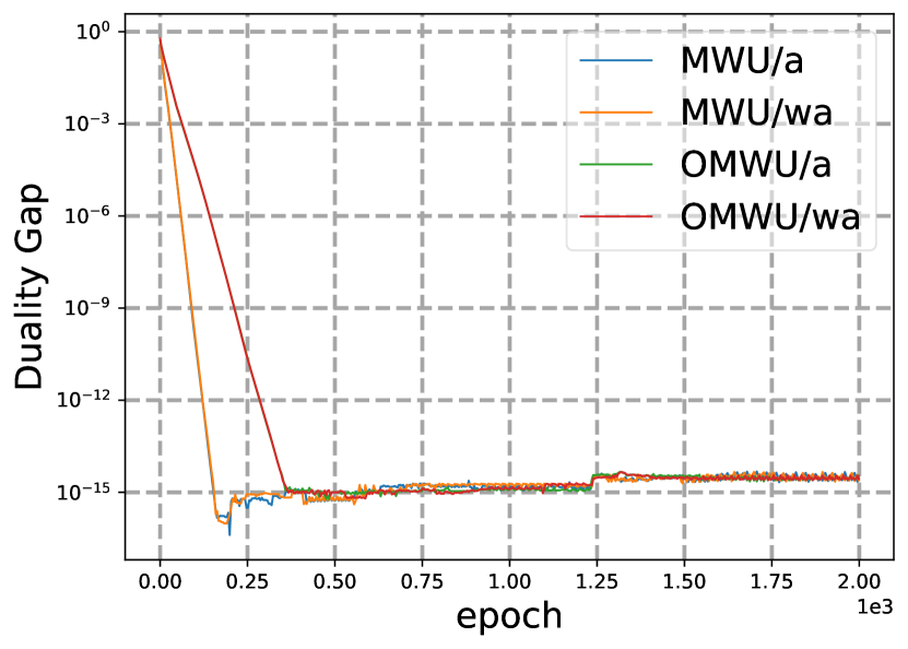
seed 18

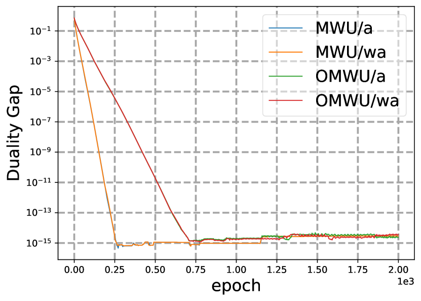
seed 19

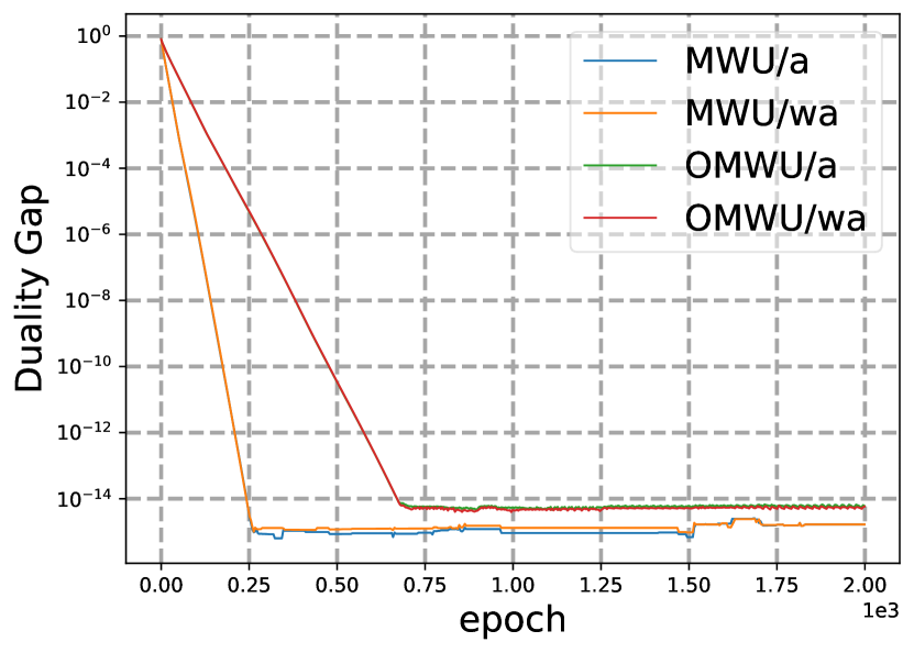
seed 20

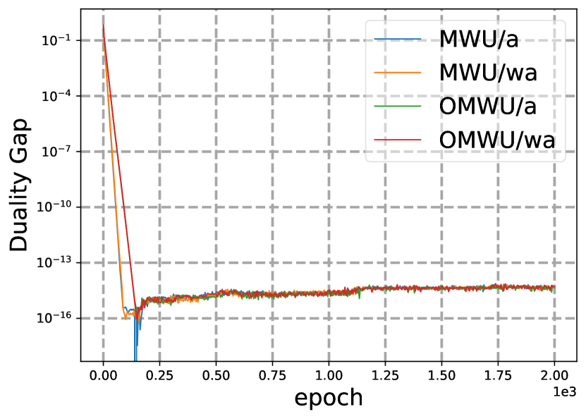
seed 21

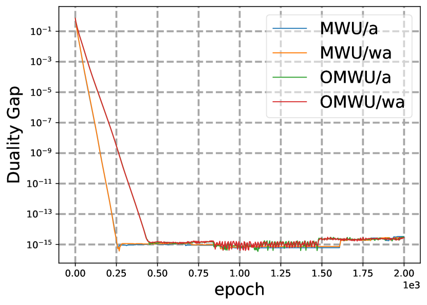
seed 22

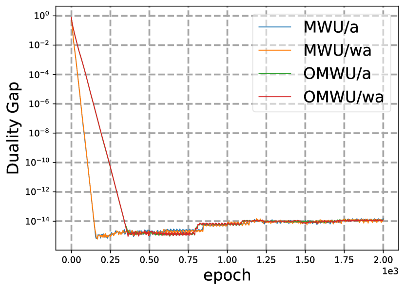
seed 23

Figure 10: Experimental results in strongly convex-concave optimization problems where $\mu=1$ and the additional regularizer is the regularizer used in [Pérolat et al., 2021].

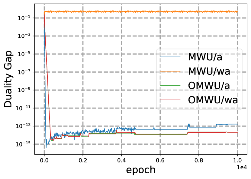
seed 0

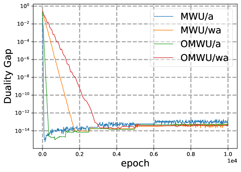
seed 1

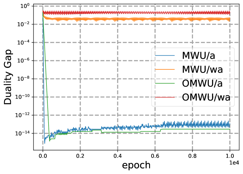
seed 2

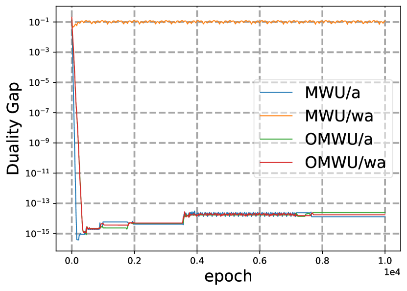
seed 3

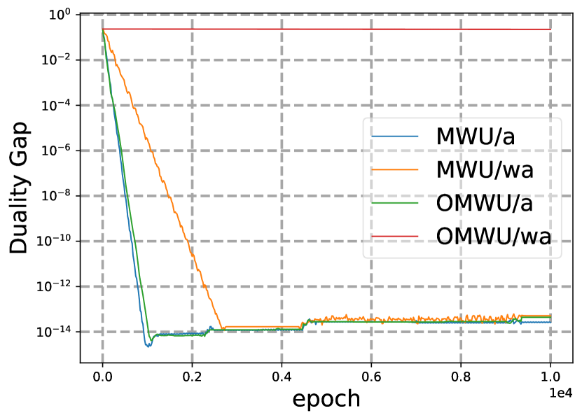
seed 4

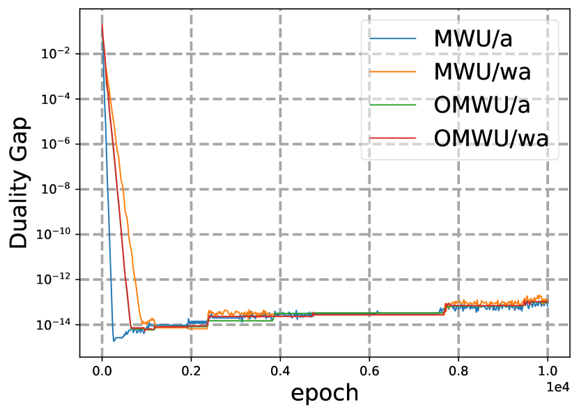
seed 5

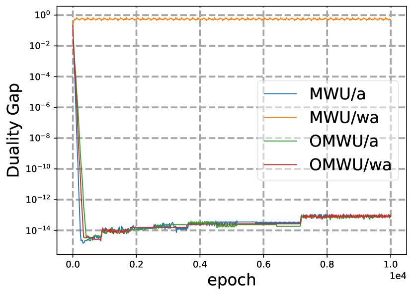
seed 6

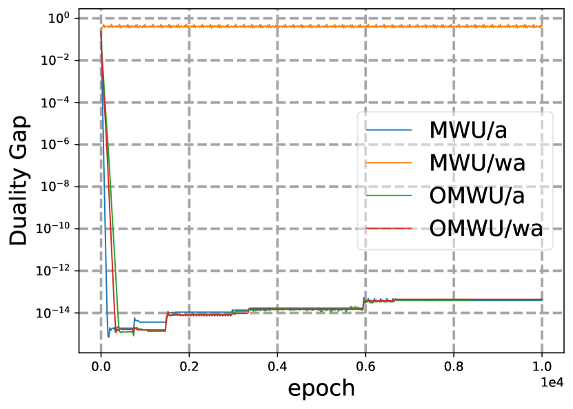
seed 7

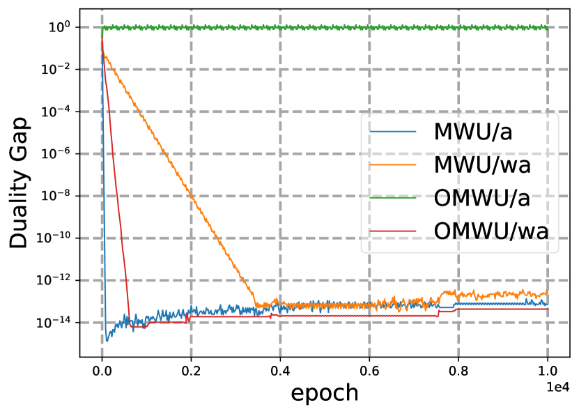
seed 8

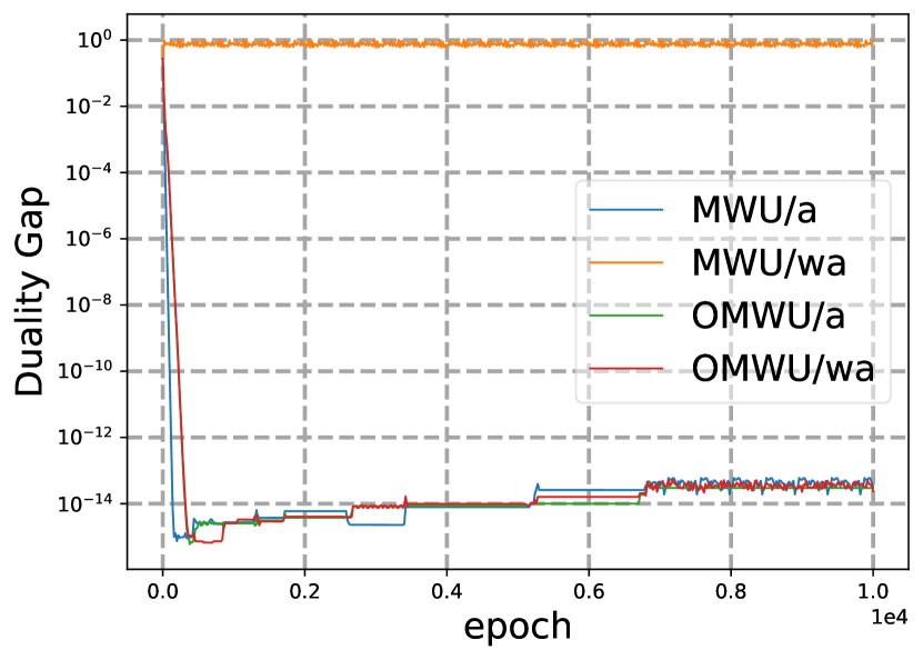
seed 9

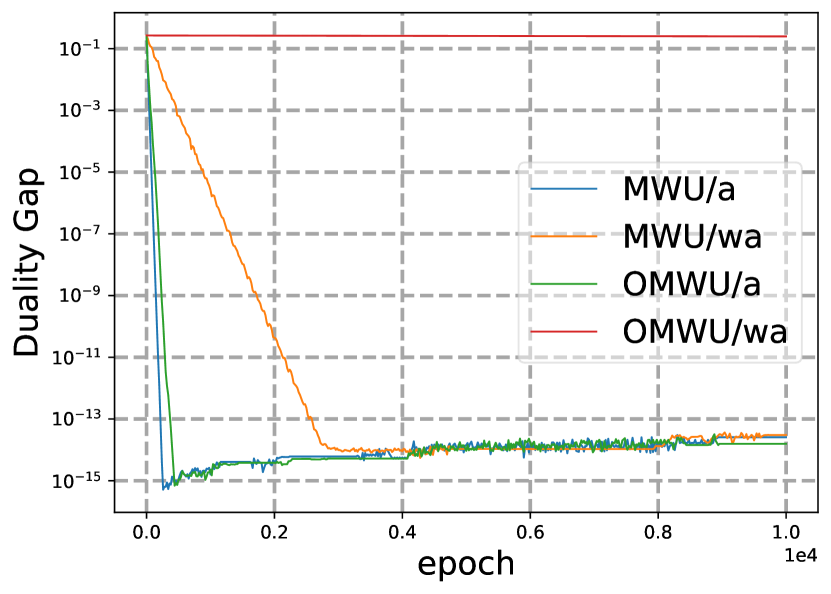
seed 10

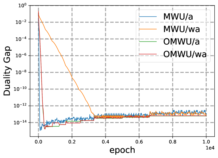
seed 11

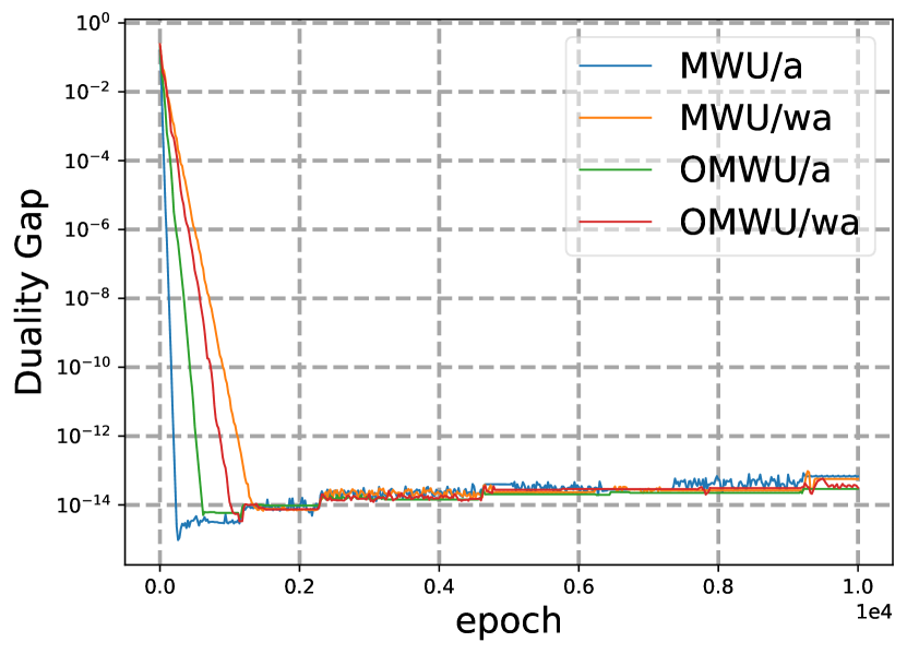
seed 12

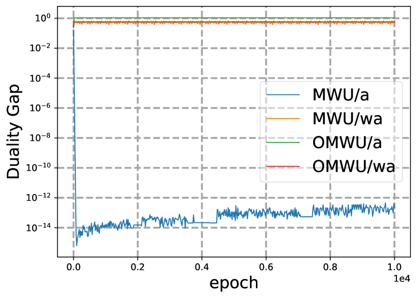
seed 13

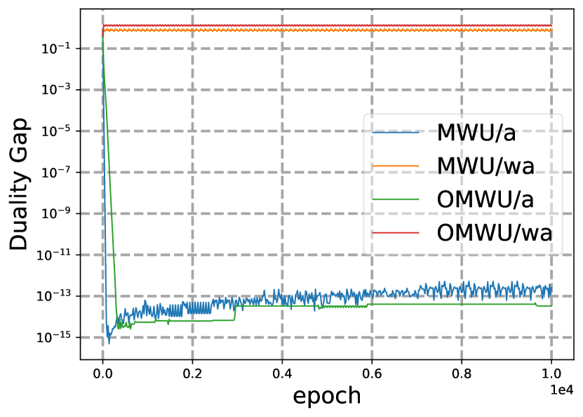
seed 14

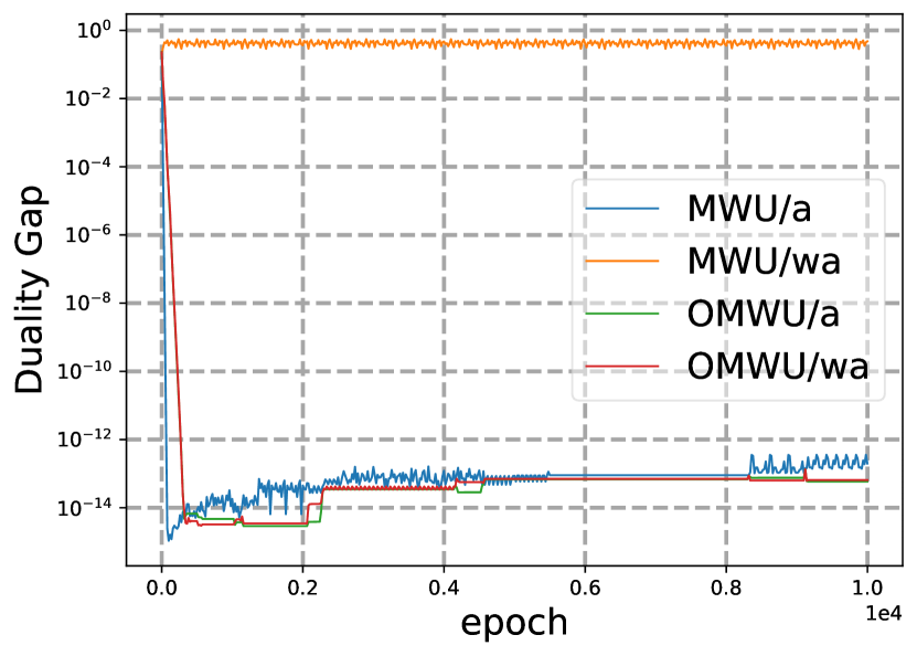
seed 15

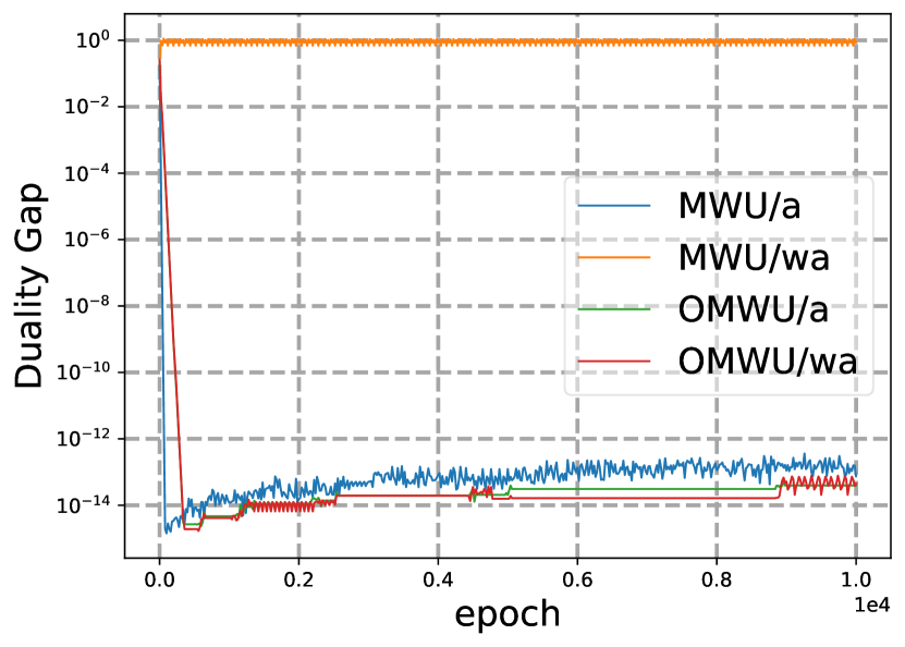
seed 16

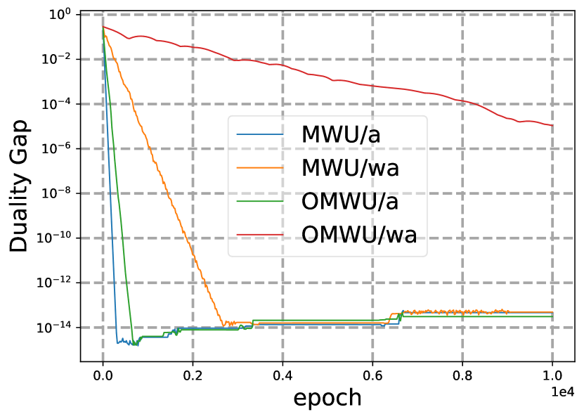
seed 17

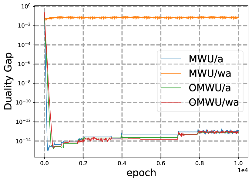
seed 18

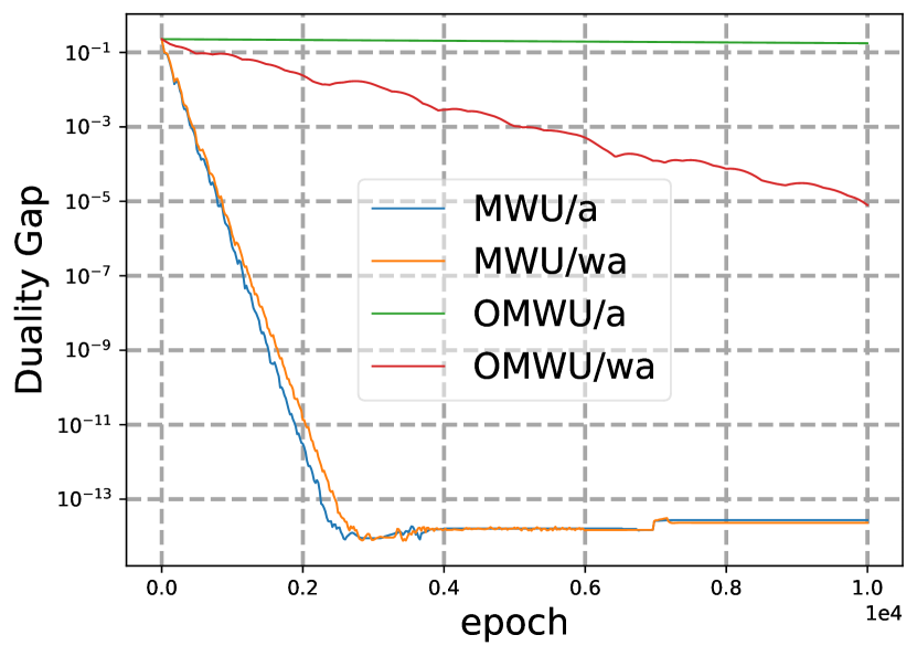
seed 19

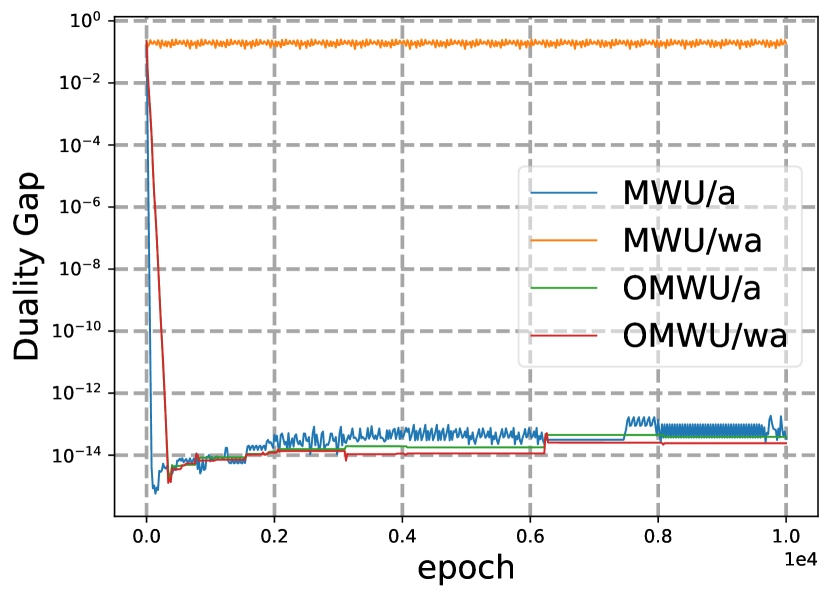
seed 20

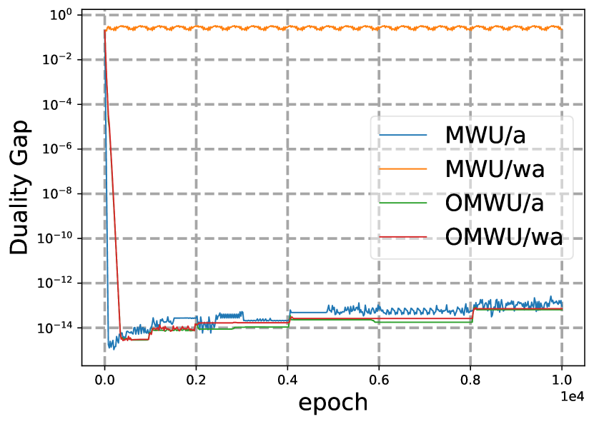
seed 21

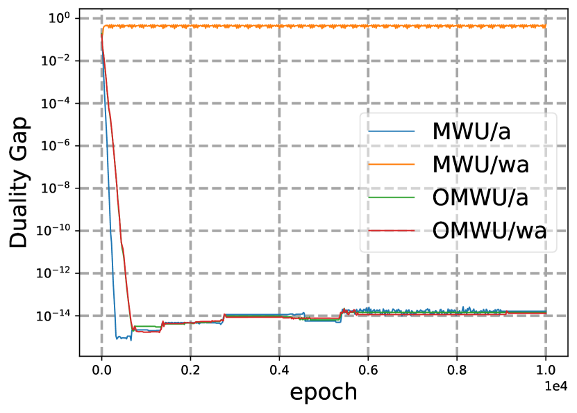
seed 22

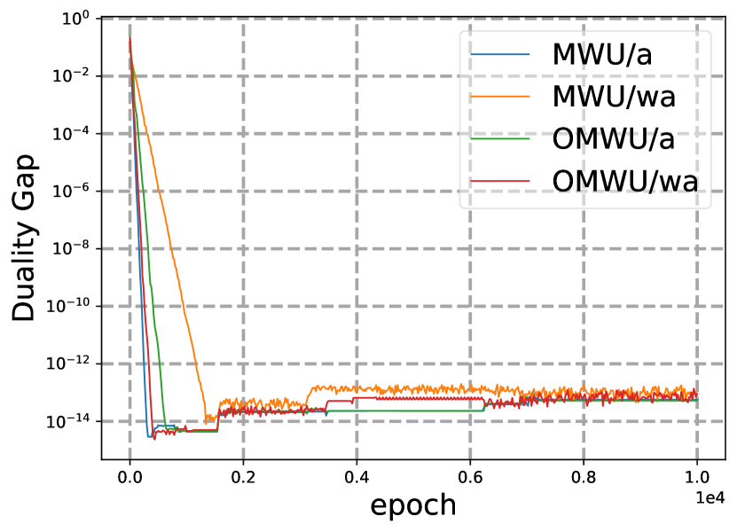
seed 23

Figure 11: Experimental results in strongly convex-concave optimization problems where $\mu=0.1$ and the additional regularizer is the regularizer used in [Pérolat et al., 2021].

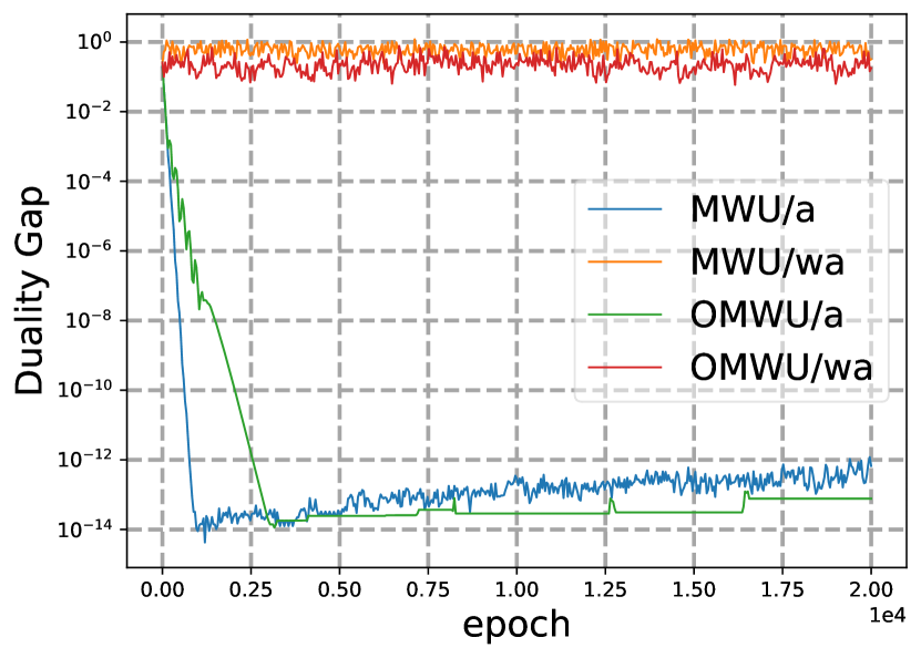
seed 0

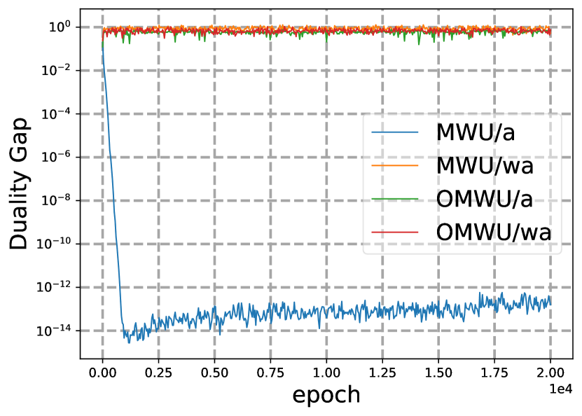
seed 1

seed 2

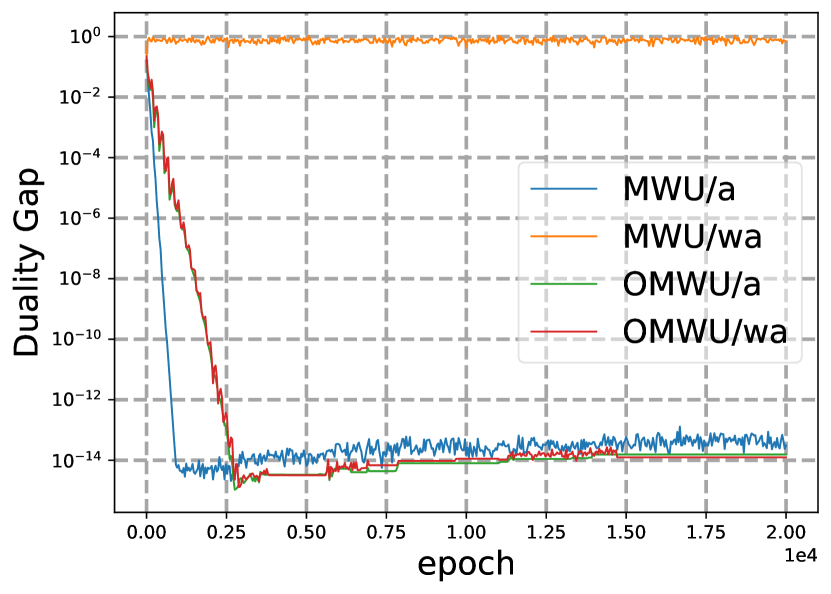
seed 3

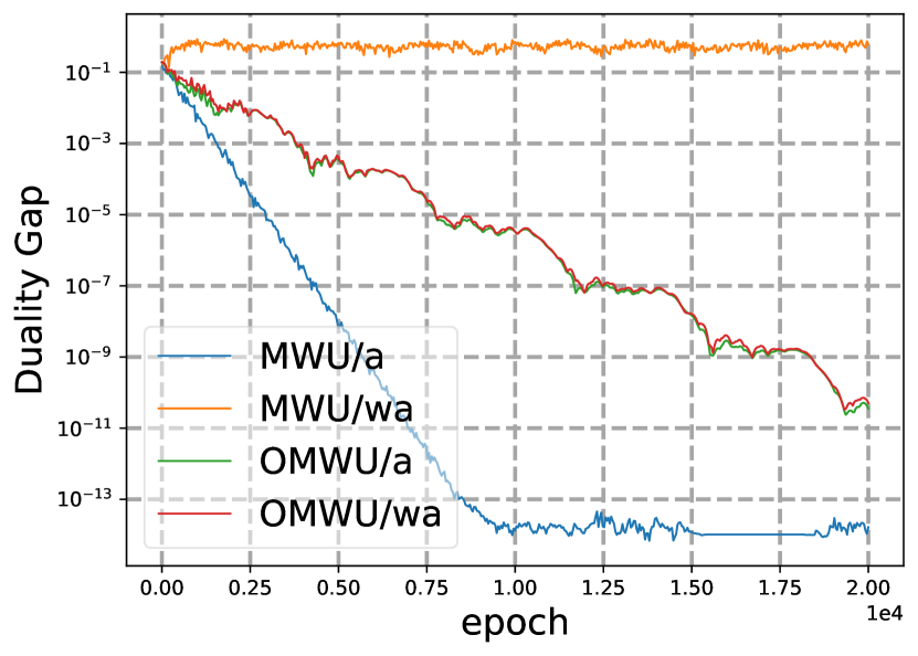
seed 4

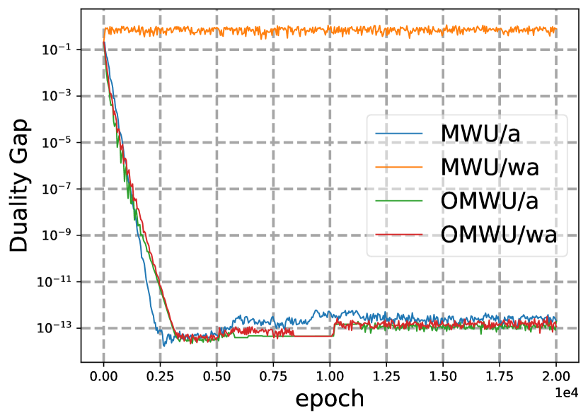
seed 5

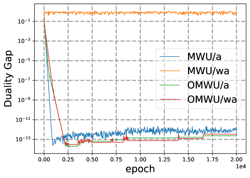
seed 6

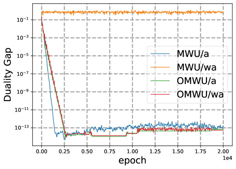
seed 7

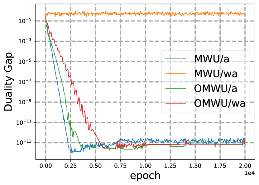
seed 8

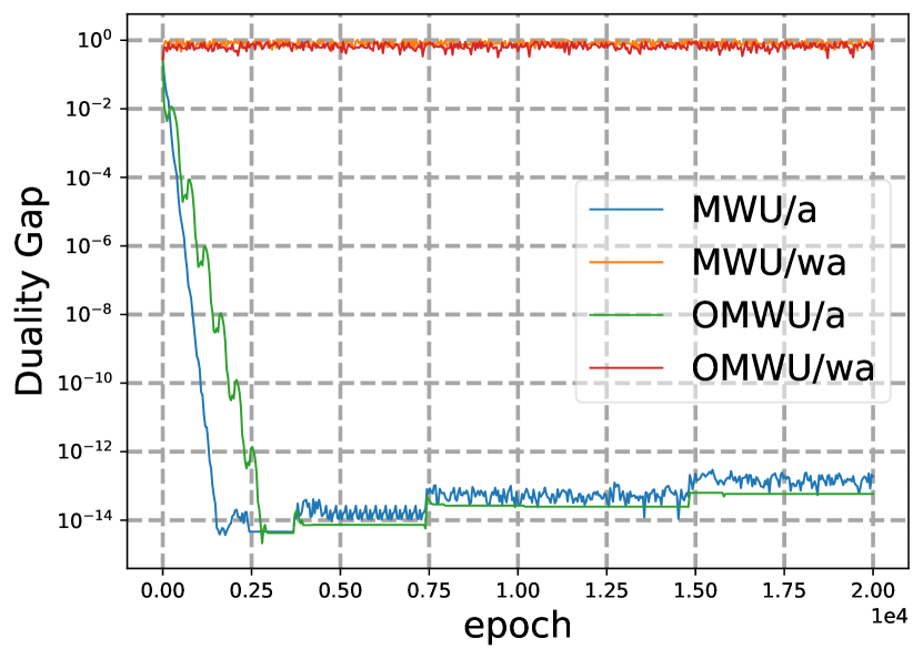
seed 9

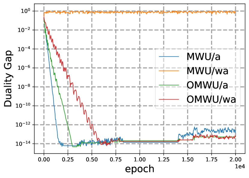
seed 10

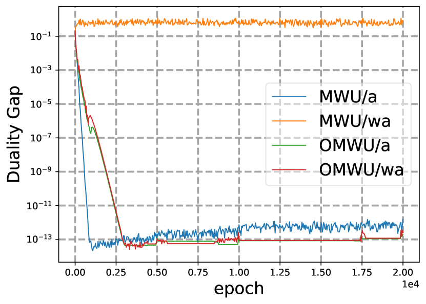
seed 11

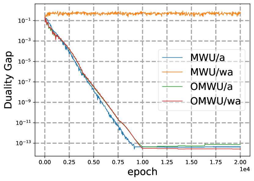
seed 12

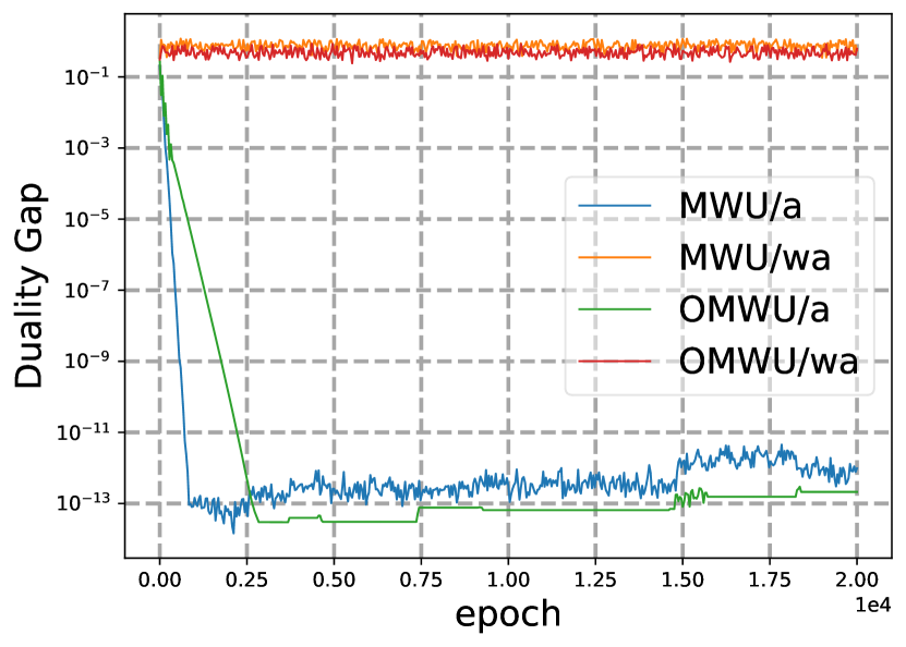
seed 13

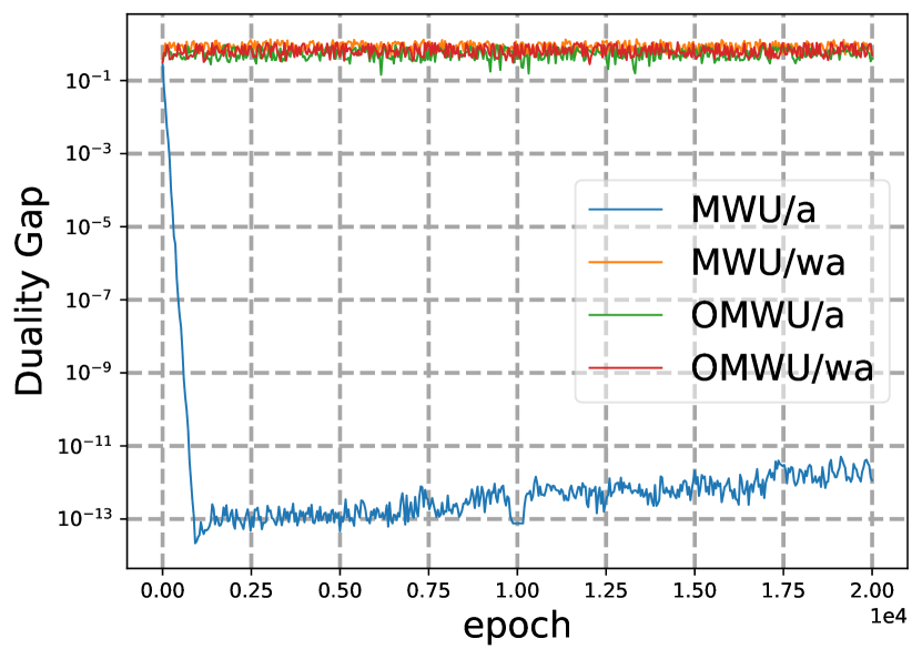
seed 14

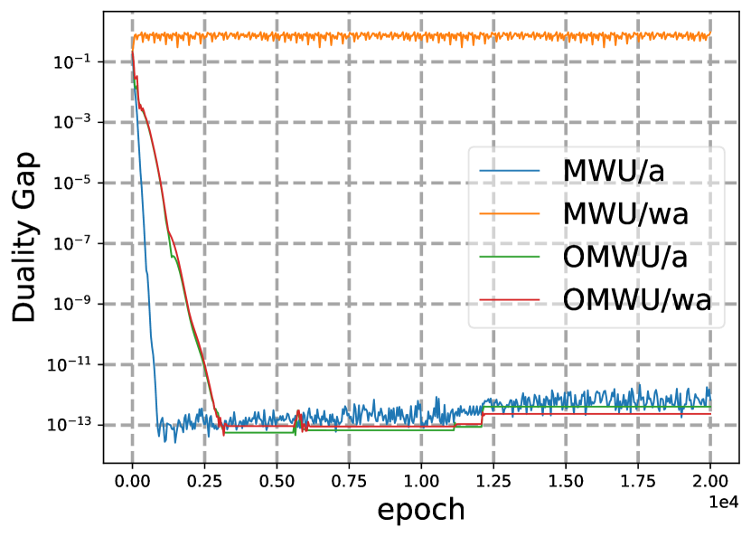
seed 15

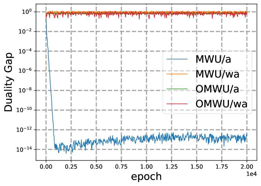
seed 16

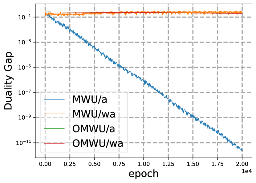
seed 17

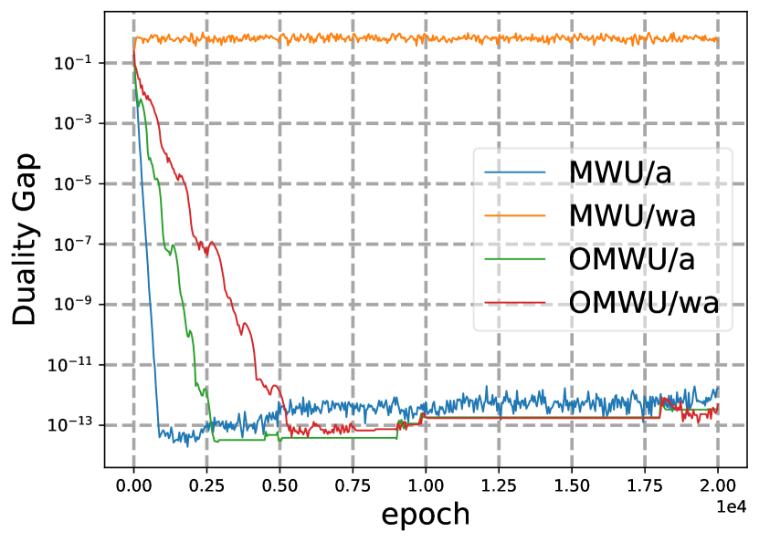
seed 18

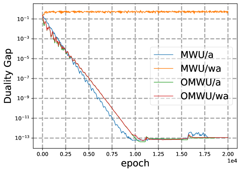
seed 19

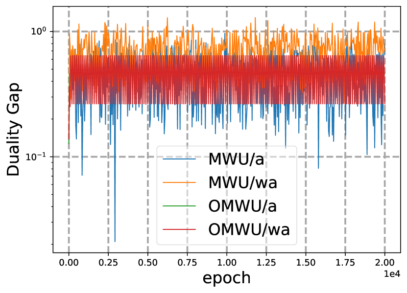
seed 20

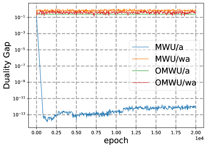
seed 21

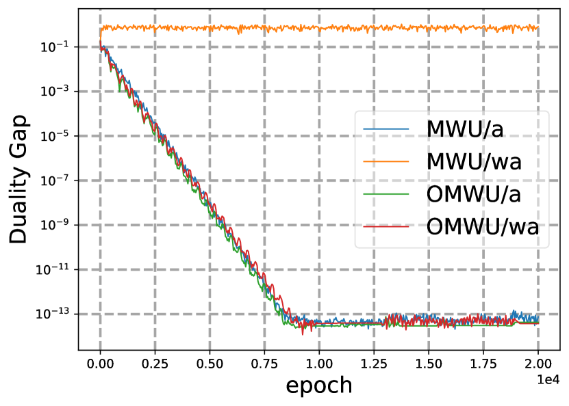
seed 22

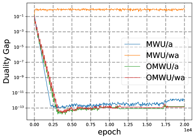
seed 23

Figure 12: Experimental results in strongly convex-concave optimization problems where $\mu=0.01$ and the additional regularizer is the regularizer used in [Pérolat et al., 2021].

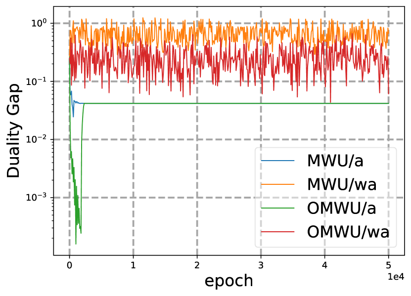
seed 0

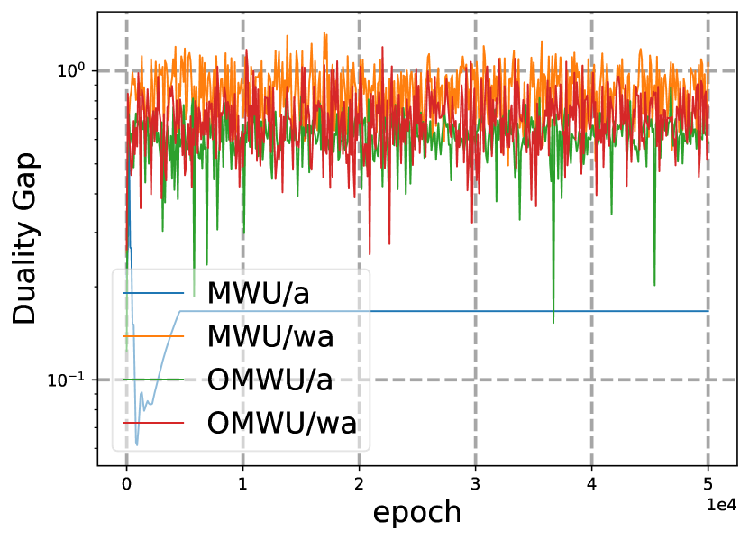
seed 1

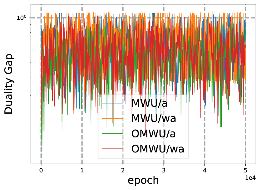
seed 2

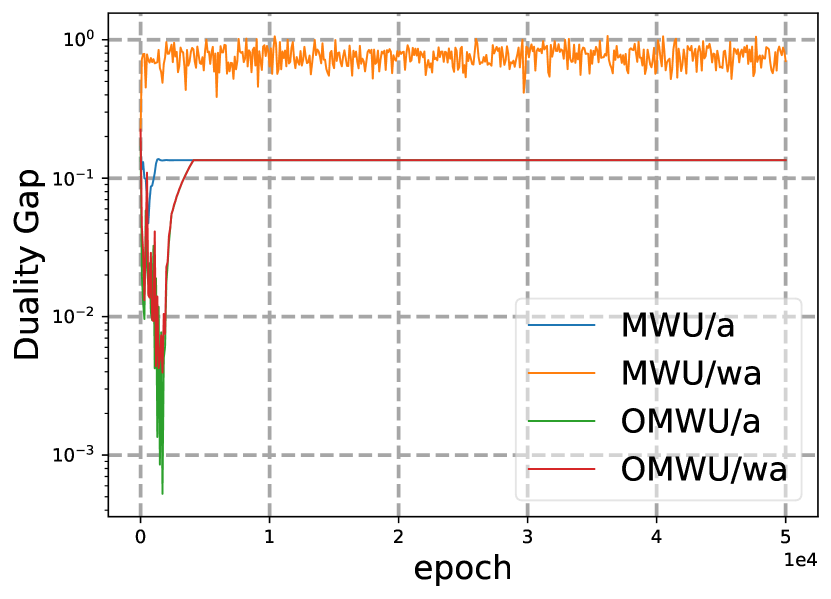
seed 3

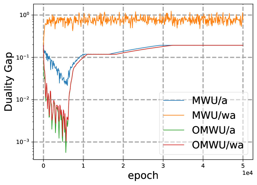
seed 4

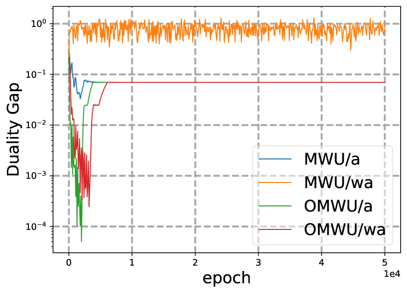
seed 5

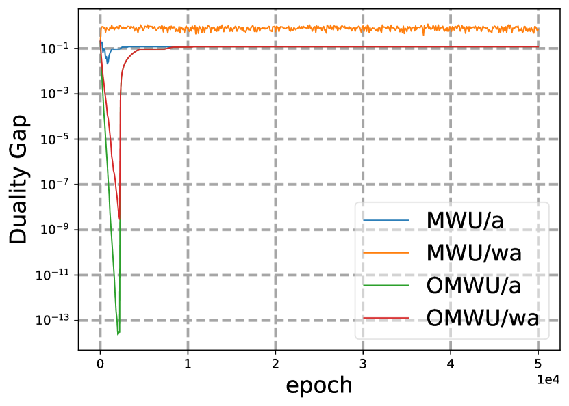
seed 6

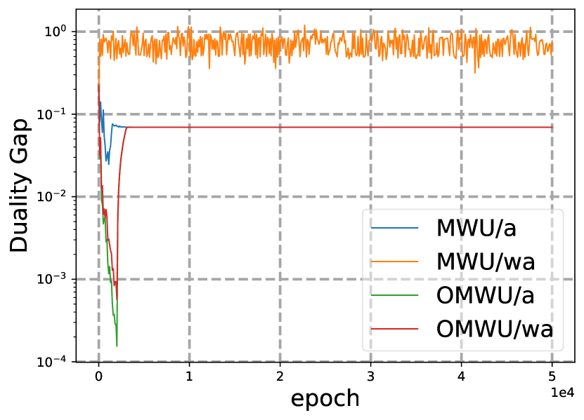
seed 7

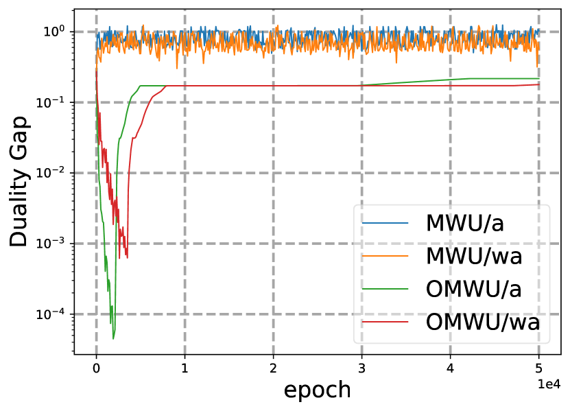
seed 8

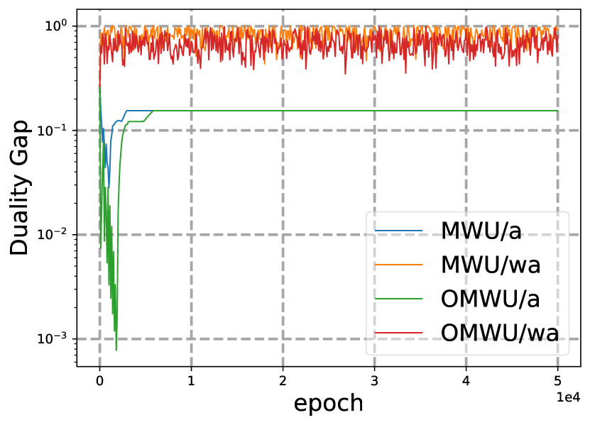
seed 9

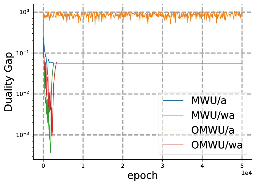
seed 10

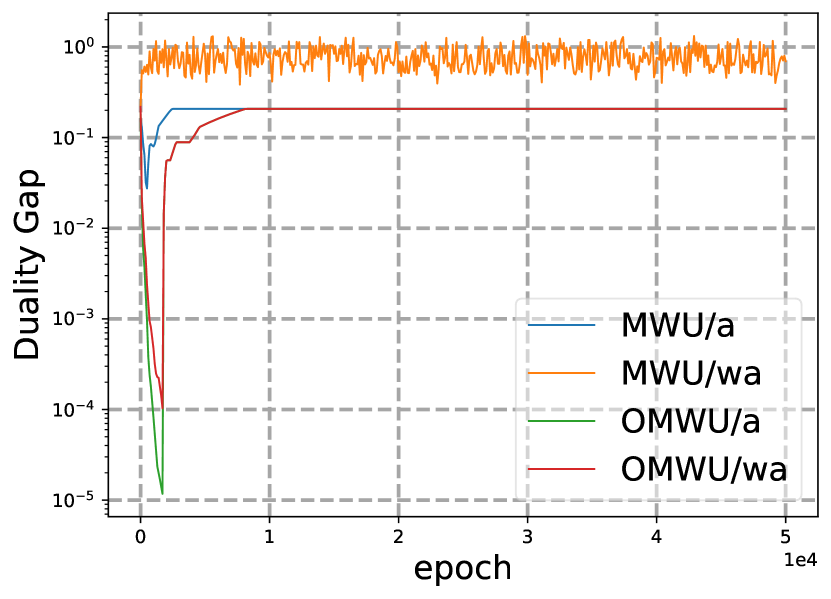
seed 11

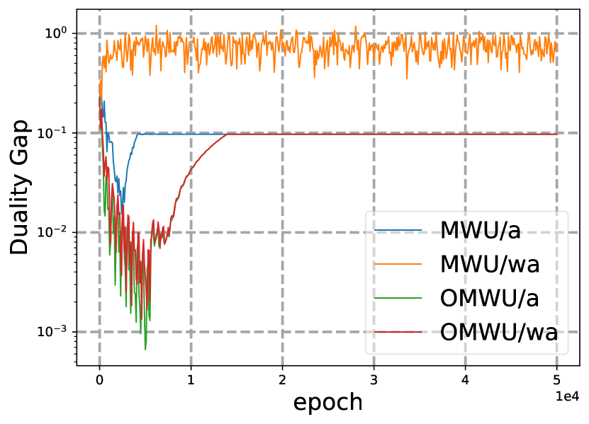
seed 12

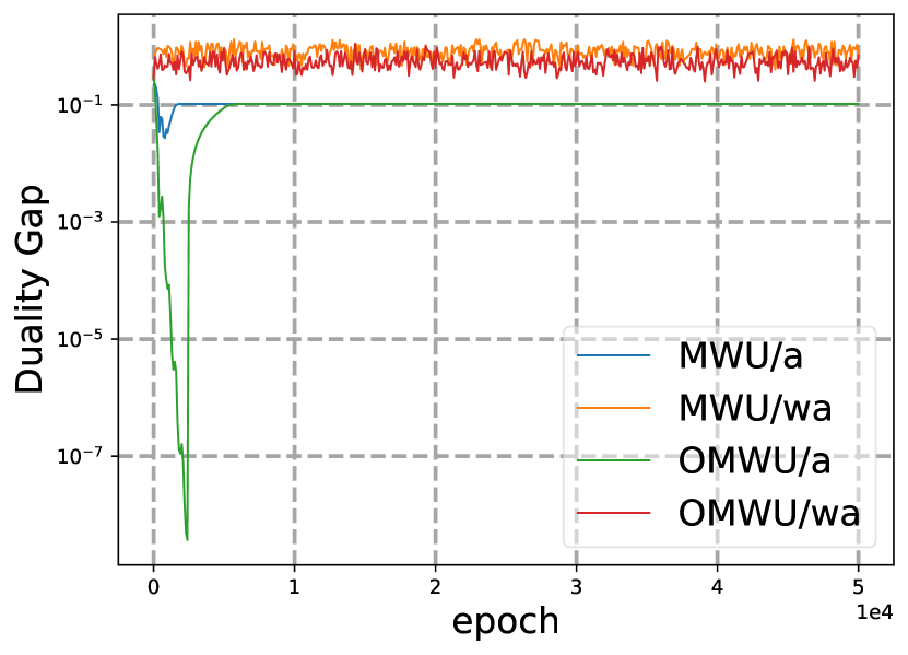
seed 13

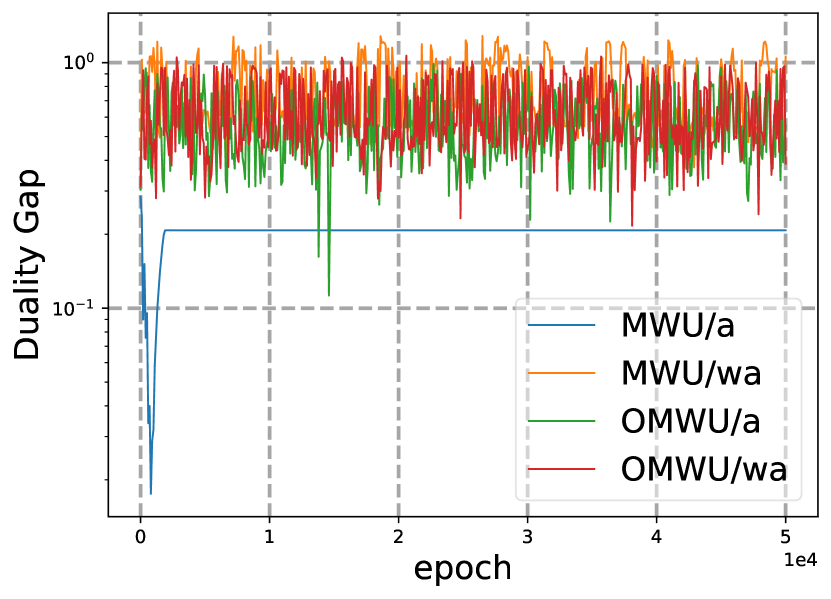
seed 14

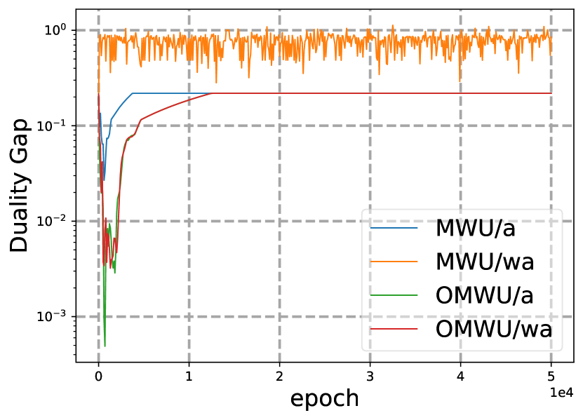
seed 15

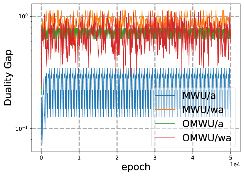
seed 16

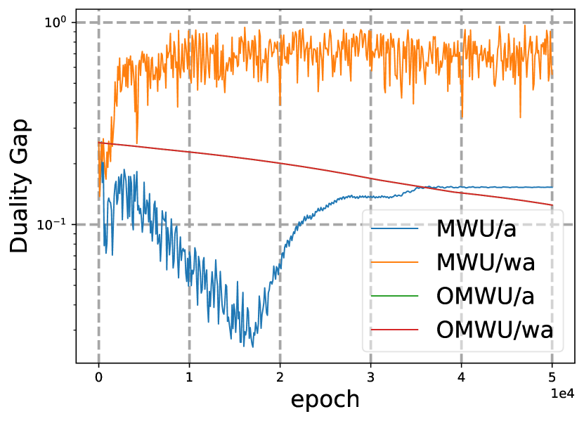
seed 17

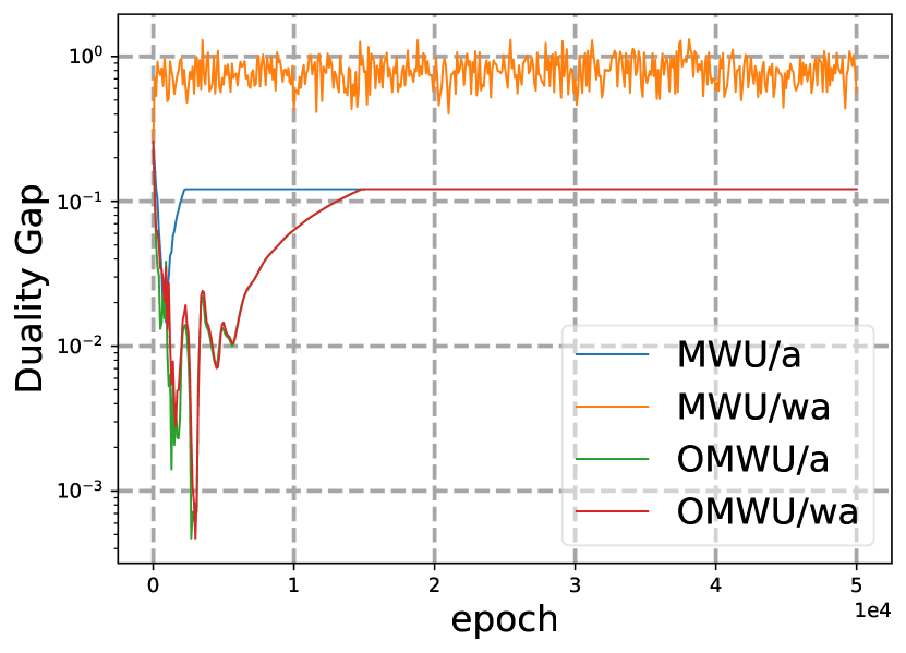
seed 18

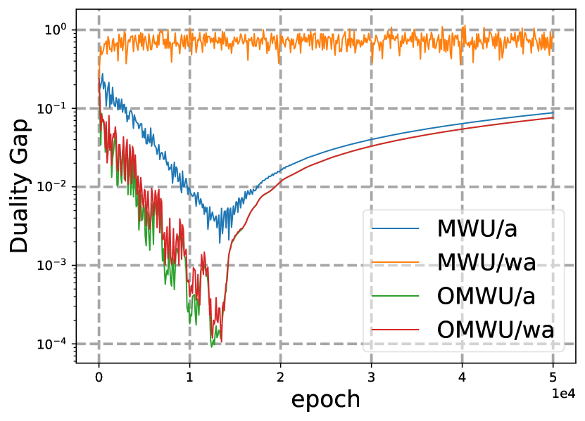
seed 19

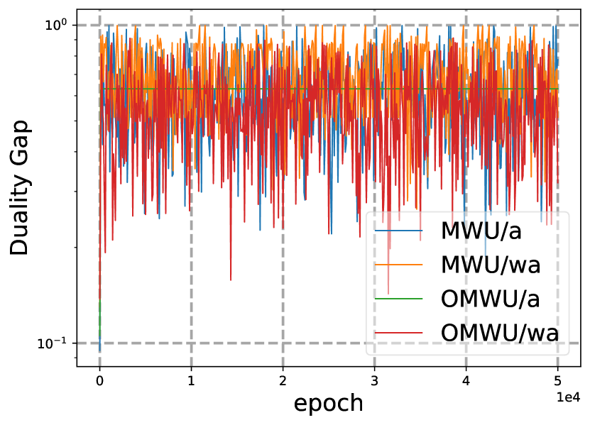
seed 20

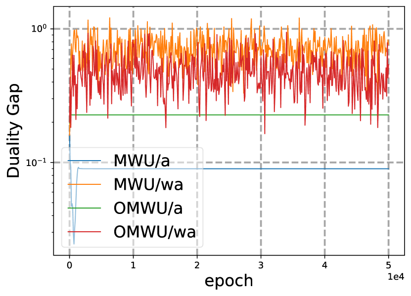
seed 21

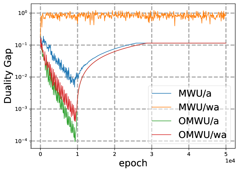
seed 22

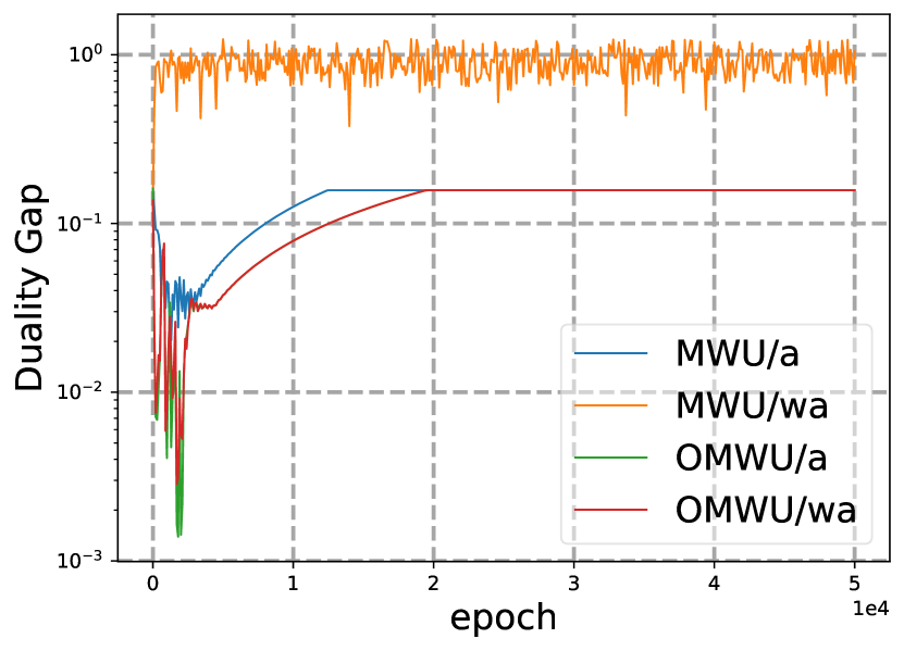
seed 23

Figure 13: Experimental results in strongly convex-concave optimization problems where $\mu=0.001$ and the additional regularizer is the regularizer used in [Pérolat et al., 2021].

Table 1: The learning rate of GDA, OGDA, MWU, and OMWU used in solving SCCPs where $\mu=1$.

Seeds	GDA/a	GDA/wa	OGDA/a	OGDA/wa	MWU/a	MWU/wa	OMWU/a	OMWU/wa
0	8	8	0.1	0.1	5	5	0.1	0.1
1	8	8	0.1	0.1	8	8	0.08	0.08
2	8	8	0.3	0.3	8	5	0.08	0.08
3	8	8	0.1	0.1	3	3	0.1	0.1
4	8	8	0.0001	0.0001	8	8	0.05	0.05
5	8	8	0.1	0.1	8	8	0.03	0.03
6	8	8	0.08	0.03	8	8	0.08	0.08
7	8	8	0.1	0.1	3	3	0.1	0.1
8	8	8	0.1	0.1	3	3	0.1	0.1
9	8	8	0.1	0.1	3	3	0.3	0.3
10	8	8	0.08	0.0001	5	5	0.1	0.1
11	8	8	0.1	0.08	3	3	0.3	0.1
12	8	8	0.05	0.03	8	8	0.08	0.05
13	8	8	0.1	0.1	5	5	0.1	0.1
14	8	8	0.1	0.3	3	3	0.1	0.1
15	8	8	0.3	0.3	3	3	0.3	0.3
16	8	8	0.3	0.3	3	3	0.1	0.1
17	8	8	0.1	0.03	3	3	0.1	0.1
18	8	8	0.1	0.3	5	5	0.1	0.1
19	8	8	0.1	0.05	8	8	0.05	0.05
20	8	8	0.1	0.3	8	8	0.05	0.05
21	8	8	0.1	0.1	3	3	0.3	0.3
22	8	8	0.1	0.08	8	8	0.08	0.08
23	8	8	0.1	0.1	5	5	0.1	0.1

Table 2: The learning rate of GDA, OGDA, MWU, and OMWU used in solving SCCPs where $\mu=0.1$.

Seeds	GDA/a	GDA/wa	OGDA/a	OGDA/wa	MWU/a	MWU/wa	OMWU/a	OMWU/wa
0	5	3	0.1	1	0.3	0.3	1	1
1	8	8	0.05	0.05	0.3	5	1	0.1
2	0.5	0.8	0.8	0.5	0.3	0.3	1	3
3	3	3	0.3	0.3	0.5	0.5	1	1
4	8	8	0.01	0.01	3	8	0.3	0.0001
5	3	3	0.3	0.3	0.8	1	0.5	0.5
6	8	8	0.0001	0.0001	0.8	0.5	0.8	1
7	5	1	0.1	1	0.5	0.3	0.8	1
8	3	3	0.1	0.3	0.3	0.8	3	0.5
9	3	3	0.1	0.1	0.5	0.3	1	1
10	8	8	0.1	0.08	0.8	8	0.8	0.0001
11	0.8	0.8	0.3	0.3	0.3	0.5	1	1
12	8	8	0.1	0.03	0.8	3	0.5	0.3
13	8	8	0.3	0.8	0.3	0.3	3	3
14	3	0.8	1	1	0.3	0.3	1	3
15	0.5	1	0.3	0.3	0.3	0.3	1	1
16	3	3	0.3	0.5	0.3	0.3	1	1
17	8	8	0.1	0.0001	1	8	0.5	0.01
18	3	3	0.3	0.1	0.5	0.8	1	0.8
19	3	8	0.1	0.01	8	8	0.0001	0.01
20	3	1	0.3	0.3	0.3	0.3	1	1
21	3	3	0.3	0.3	0.3	0.3	1	1
22	0.8	8	0.0001	0.0001	1	0.8	0.5	0.5
23	5	5	0.1	0.1	1	0.8	0.5	0.8

Table 3: The learning rate of GDA, OGDA, MWU, and OMWU used in solving SCCPs where $\mu=0.01$.

Seeds	GDA/a	GDA/wa	OGDA/a	OGDA/wa	MWU/a	MWU/wa	OMWU/a	OMWU/wa
0	3	0.5	0.1	1	0.3	0.3	1	3
1	8	8	0.05	0.05	0.3	0.3	3	3
2	0.5	0.8	0.8	0.8	0.08	0.1	5	5
3	3	8	0.3	0.08	0.3	0.3	1	1
4	8	8	0.03	0.01	3	3	0.1	0.1
5	3	3	0.3	0.3	0.8	0.8	0.8	0.8
6	8	8	0.0001	0.0001	0.3	0.3	1	1
7	3	0.3	0.3	1	0.5	0.3	1	1
8	3	1	0.3	0.5	0.8	1	0.8	0.5
9	3	3	0.1	0.1	0.5	0.3	1	3
10	5	8	0.1	0.0001	0.5	0.8	1	0.5
11	3	3	0.3	0.3	0.3	0.5	1	1
12	5	8	0.1	0.05	3	3	0.3	0.3
13	0.8	0.5	0.3	1	0.3	0.3	1	3
14	0.5	0.5	1	1	0.3	0.1	5	5
15	3	1	0.3	0.3	0.3	0.3	1	1
16	1	1	0.3	0.5	0.3	0.3	3	3
17	5	8	0.1	0.0001	8	8	0.0001	0.0001
18	3	5	0.3	0.1	0.3	1	1	0.5
19	3	8	0.1	0.01	3	3	0.3	0.3
20	3	1	0.3	0.3	0.1	0.1	5	5
21	3	3	0.3	0.3	0.3	0.3	3	3
22	8	8	0.0001	0.0001	3	1	0.3	0.3
23	3	3	0.3	0.1	0.8	0.5	0.8	0.8

Table 4: The learning rate of GDA, OGDA, MWU, and OMWU used in solving SCCPs where $\mu=0.001$.

Seeds	GDA/a	GDA/wa	OGDA/a	OGDA/wa	MWU/a	MWU/wa	OMWU/a	OMWU/wa
0	3	0.5	0.1	1	0.3	0.3	1	3
1	8	8	0.05	0.05	0.3	0.3	3	3
2	0.5	0.8	0.8	0.8	0.08	0.1	8	5
3	3	8	0.3	0.08	0.3	0.3	1	1
4	8	8	0.03	0.01	3	3	0.3	0.3
5	3	3	0.3	0.3	0.8	0.8	0.8	0.5
6	8	8	0.0001	0.0001	0.3	0.3	1	1
7	3	0.3	0.3	1	0.5	0.3	1	1
8	3	1	0.3	0.5	0.01	0.8	0.8	0.5
9	3	3	0.1	0.1	0.5	0.3	1	3
10	5	8	0.1	0.0001	0.5	0.8	1	0.8
11	3	3	0.3	0.3	0.3	0.5	1	1
12	5	8	0.1	0.05	1	3	0.3	0.3
13	0.8	0.5	0.3	1	0.3	0.3	1	3
14	0.5	0.5	1	1	0.3	0.08	5	5
15	3	3	0.3	0.3	0.3	0.3	1	1
16	1	1	0.3	0.5	0.3	0.3	3	3
17	5	8	0.1	0.0001	8	8	0.0001	0.0001
18	3	5	0.3	0.1	0.3	1	0.5	0.5
19	3	8	0.3	0.01	3	3	0.3	0.3
20	3	1	0.3	0.3	0.08	0.08	5	5
21	3	3	0.3	0.3	0.3	0.3	3	3
22	8	8	0.0001	0.0001	3	1	0.3	0.3
23	3	3	0.3	0.1	0.8	0.8	0.8	0.8

Appendix I Hyper-Parameters in Experiments

In this section, we show the hyperparameters used in Section 6 and Appendix G. The results are shown in Table 5, Table 6, Table 7, Table 8, Table 9, Table 10, Table 11, Table 12, Table 13, Table 14, Table 15, Table 16, Table 17, Table 18, and Table 19. For DOGDA, we use the dilated Euclidean square norm proposed by Kroer et al. [2020]. In all tables, the notation lr represents the learning rate.

Table 5: The hyperparameter of RTRM+ used in 5x5 generated NFGs.

Seeds	0	1	2	3	4	5	6	7	8	9
$\mu$	0.1	0.5	0.5	0.5	0.5	0.1	0.5	0.1	0.1	0.1
$T$	50	5	5	5	5	10	5	5	5	1
$N$	40	400	400	400	400	200	400	400	400	2000
Seeds	10	11	12	13	14	15	16	17	18	19
$\mu$	0.1	0.5	0.1	0.5	0.5	0.1	0.5	0.5	0.1	0.5
$T$	10	5	10	5	5	1	5	10	10	5
$N$	200	400	200	400	400	2000	400	200	200	400

Table 6: The hyperparameter of RTRM+ without alternating update used in 5x5 generated NFGs.

Seeds	0	1	2	3	4	5	6	7	8	9
$\mu$	1.0	0.5	0.5	0.5	0.5	1.0	1.0	1.0	1.0	0.1
$T$	10	10	10	5	10	5	5	10	5	1
$N$	200	200	200	400	200	400	400	200	400	2000
Seeds	10	11	12	13	14	15	16	17	18	19
$\mu$	1.0	0.5	1.0	0.5	2.0	0.1	1.0	1.0	1.0	0.5
$T$	5	10	5	10	5	1	5	10	5	5
$N$	400	200	400	200	400	2000	400	200	400	400

Table 7: The hyperparameter of OMWU used in 5x5 generated NFGs.

Seeds	0	1	2	3	4	5	6	7	8	9
lr	0.8	1	1	0.8	1	1	1	1	1	5
Seeds	10	11	12	13	14	15	16	17	18	19
lr	0.5	0.8	1	1	1	5	1	1	1	1

Table 8: The hyperparameter of OGDA used in 5x5 generated NFGs.

Seeds	0	1	2	3	4	5	6	7	8	9
lr	0.3	0.5	0.3	0.5	0.5	0.3	0.3	0.3	0.5	0.5
Seeds	10	11	12	13	14	15	16	17	18	19
lr	0.3	0.3	0.3	0.5	0.3	8	0.5	0.08	0.3	0.5

Table 9: The hyperparameter of R-NaD used in 5x5 generated NFGs.

Seeds	0	1	2	3	4	5	6	7	8	9
$\mu$	0.01	0.01	0.01	0.01	0.005	0.005	0.01	0.005	0.005	0.001
lr	1	1	1	5	5	5	1	5	5	0.5
$T$	100	100	100	100	100	100	100	100	100	100
$N$	20	20	20	20	20	20	20	20	20	20
Seeds	10	11	12	13	14	15	16	17	18	19
$\mu$	0.01	0.05	0.01	0.05	0.005	0.001	0.005	0.01	0.05	0.01
lr	1	1	5	0.5	1	0.5	5	1	0.5	5
$T$	100	100	100	100	100	100	100	100	100	100
$N$	20	20	20	20	20	20	20	20	20	20

Table 10: The hyperparameter of OR-NaD used in 5x5 generated NFGs.

Seeds	0	1	2	3	4	5	6	7	8	9
$\mu$	0.01	0.005	0.005	0.01	0.01	0.005	0.001	0.01	0.001	0.001
lr	0.5	0.5	0.5	1	1	1	1	5	1	0.5
$T$	100	100	100	100	100	100	100	100	100	100
$N$	20	20	20	20	20	20	20	20	20	20
Seeds	10	11	12	13	14	15	16	17	18	19
$\mu$	0.01	0.05	0.01	0.01	0.001	0.001	0.005	0.01	0.01	0.001
lr	1	1	1	1	1	0.5	1	1	1	1
$T$	100	100	100	100	100	100	100	100	100	100
$N$	20	20	20	20	20	20	20	20	20	20

Table 11: The hyperparameter of RTRM+ used in 10x10 generated NFGs.

Seeds	0	1	2	3	4	5	6	7	8	9
$\mu$	0.1	0.1	0.1	0.1	0.5	0.5	0.5	0.1	0.1	0.1
$T$	10	10	5	10	10	5	10	50	10	50
$N$	200	200	400	200	200	400	200	40	200	40
Seeds	10	11	12	13	14	15	16	17	18	19
$\mu$	0.1	0.5	0.5	0.5	0.1	0.1	0.1	0.1	0.1	0.1
$T$	50	10	10	5	50	50	10	50	50	50
$N$	40	200	200	400	40	40	200	40	40	40

Table 12: The hyperparameter of RTRM+ without alternating update used in 10x10 generated NFGs.

Seeds	0	1	2	3	4	5	6	7	8	9
$\mu$	0.5	0.5	1.0	1.0	2.0	2.0	2.0	0.5	2.0	2.0
$T$	50	10	10	10	5	10	10	50	5	5
$N$	40	200	200	200	400	200	200	40	400	400
Seeds	10	11	12	13	14	15	16	17	18	19
$\mu$	0.5	2.0	2.0	2.0	0.5	1.0	1.0	2.0	0.5	0.5
$T$	50	5	10	5	10	5	5	5	50	50
$N$	40	400	200	400	200	400	400	400	40	40

Table 13: The hyperparameter of OMWU used in 10x10 generated NFGs.

Seeds	0	1	2	3	4	5	6	7	8	9
lr	0.8	1	1	0.8	1	1	1	1	1	5
Seeds	10	11	12	13	14	15	16	17	18	19
lr	0.5	1	1	1	0.8	1	1	1	0.8	1

Table 14: The hyperparameter of OGDA used in 10x10 generated NFGs.

Seeds	0	1	2	3	4	5	6	7	8	9
lr	0.3	0.1	0.3	0.1	0.1	0.1	0.1	0.1	0.3	0.1
Seeds	10	11	12	13	14	15	16	17	18	19
lr	0.1	0.1	0.1	0.1	0.3	0.1	0.3	0.1	0.1	0.1

Table 15: The hyperparameter of R-NaD used in 10x10 generated NFGs.

Seeds	0	1	2	3	4	5	6	7	8	9
$\mu$	0.005	0.01	0.005	0.005	0.005	0.05	0.05	0.005	0.05	0.01
lr	1	1	1	1	1	1	0.5	1	0.5	1
$T$	500	100	500	500	100	100	100	500	100	500
$N$	4	20	4	4	20	20	20	4	20	4
Seeds	10	11	12	13	14	15	16	17	18	19
$\mu$	0.005	0.005	0.01	0.05	0.005	0.005	0.1	0.01	0.01	0.005
lr	1	1	0.5	0.5	5	1	1	1	5	1
$T$	500	100	500	100	100	500	100	100	100	500
$N$	4	20	4	20	20	4	20	20	20	4

Table 16: The hyperparameter of OR-NaD used in 10x10 generated NFGs.

Seeds	0	1	2	3	4	5	6	7	8	9
$\mu$	0.005	0.005	0.005	0.01	0.01	0.01	0.001	0.005	0.05	0.01
lr	1	1	1	1	1	1	1	1	1	1
$T$	500	500	500	100	100	100	100	100	100	100
$N$	4	4	4	20	20	20	20	20	20	20
Seeds	10	11	12	13	14	15	16	17	18	19
$\mu$	0.001	0.005	0.01	0.05	0.001	0.005	0.05	0.005	0.005	0.005
lr	1	1	1	0.5	1	1	1	1	1	1
$T$	1000	100	100	100	500	500	100	100	500	500
$N$	2	20	20	20	4	4	20	20	4	4

Table 17: The hyperparameters of RTCFR+ used in EFGs.

	Kuhn Poker	Goofspiel(4)	Liars Dice(4)	Leduc Poker	Goofspiel(5)	Liars Dice(5)	Liars Dice(6)
$\mu$	0.5	0.5	0.05	0.1	0.1	0.05	0.01
$T$	5	5	50	100	50	100	2000
$N$	400	400	40	100	100	50	15

Table 18: The hyperparameters of R-NaD used in EFGs.

	Kuhn Poker	Goofspiel(4)	Liars Dice(4)	Leduc Poker	Goofspiel(5)	Liars Dice(5)	Liars Dice(6)
$\mu$	0.1	0.1	0.01	0.1	0.01	0.01	0.01
$T$	50	5	100	1000	500	500	5000
$N$	40	400	20	10	10	10	6
lr	1	5	10	5	1	10	10

Table 19: The hyperparameters of DOGDA used in EFGs.

	Kuhn Poker	Goofspiel(4)	Liars Dice(4)	Leduc Poker	Goofspiel(5)	Liars Dice(5)	Liars Dice(6)
lr	2	2	10	10	2	5	0.5

References

• Goodfellow et al. [2014] Ian J. Goodfellow, Jean Pouget-Abadie, Mehdi Mirza, Bing Xu, David Warde-Farley, Sherjil Ozair, Aaron C. Courville, and Yoshua Bengio. Generative adversarial nets. In Proceedings of the 24th International Conference on Neural Information Processing Systems, pages 2672–2680, 2014.
• Osborne et al. [2004] Martin J Osborne et al. An introduction to game theory, volume 3. Oxford university press New York, 2004.
• Busoniu et al. [2008] Lucian Busoniu, Robert Babuska, and Bart De Schutter. A comprehensive survey of multiagent reinforcement learning. IEEE Trans. Syst. Man Cybern. Part C, 38(2):156–172, 2008.
• Bailey and Piliouras [2018] James P. Bailey and Georgios Piliouras. Multiplicative weights update in zero-sum games. In Proceedings of the 19th ACM Conference on Economics and Computation, pages 321–338, 2018.
• Mertikopoulos et al. [2018] Panayotis Mertikopoulos, Christos H. Papadimitriou, and Georgios Piliouras. Cycles in adversarial regularized learning. In Proceedings of the 29th Annual ACM-SIAM Symposium on Discrete Algorithms, pages 2703–2717, 2018.
• Pérolat et al. [2021] Julien Pérolat, Rémi Munos, Jean-Baptiste Lespiau, Shayegan Omidshafiei, Mark Rowland, Pedro A. Ortega, Neil Burch, Thomas W. Anthony, David Balduzzi, Bart De Vylder, Georgios Piliouras, Marc Lanctot, and Karl Tuyls. From poincaré recurrence to convergence in imperfect information games: Finding equilibrium via regularization. In Proceedings of the 38th International Conference on Machine Learning, pages 8525–8535, 2021.
• Wei et al. [2021] Chen-Yu Wei, Chung-Wei Lee, Mengxiao Zhang, and Haipeng Luo. Linear last-iterate convergence in constrained saddle-point optimization. In Proceedings of the 9th International Conference on Learning Representations, 2021.
• Lee et al. [2021] Chung-Wei Lee, Christian Kroer, and Haipeng Luo. Last-iterate convergence in extensive-form games. In Proceedings of the 35th International Conference on Neural Information Processing, pages 14293–14305, 2021.
• Bauer et al. [2019] Johann Bauer, Mark Broom, and Eduardo Alonso. The stabilization of equilibria in evolutionary game dynamics through mutation: mutation limits in evolutionary games. In Proceedings of the Royal Society A, 475(2231):20190355, 2019.
• Pérolat et al. [2022] Julien Pérolat, Bart De Vylder, Daniel Hennes, Eugene Tarassov, Florian Strub, Vincent de Boer, Paul Muller, Jerome T Connor, Neil Burch, Thomas Anthony, et al. Mastering the game of stratego with model-free multiagent reinforcement learning. Science, 378(6623):990–996, 2022.
• Abe et al. [2022a] Kenshi Abe, Mitsuki Sakamoto, and Atsushi Iwasaki. Mutation-driven follow the regularized leader for last-iterate convergence in zero-sum games. In Proceedings of the 38th Conference on Uncertainty in Artificial Intelligence, pages 1–10, 2022a.
• Abe et al. [2022b] Kenshi Abe, Kaito Ariu, Mitsuki Sakamoto, Kentaro Toyoshima, and Atsushi Iwasaki. Last-iterate convergence with full- and noisy-information feedback in two-player zero-sum games. CoRR, abs/2208.09855, 2022b.
• Bowling et al. [2015] Michael Bowling, Neil Burch, Michael Johanson, and Oskari Tammelin. Heads-up limit hold’em poker is solved. Science, 347(6218):145–149, 2015.
• Farina et al. [2021a] Gabriele Farina, Christian Kroer, and Tuomas Sandholm. Faster game solving via predictive blackwell approachability: Connecting regret matching and mirror descent. In Proceedings of the 35th AAAI Conference on Artificial Intelligence, pages 5363–5371, 2021a.
• Zinkevich et al. [2007] Martin Zinkevich, Michael Johanson, Michael Bowling, and Carmelo Piccione. Regret minimization in games with incomplete information. In Proceedings of the 20th International Conference on Neural Information Processing Systems, pages 1729–1736, 2007.
• Freund and Schapire [1999] Yoav Freund and Robert E Schapire. Adaptive game playing using multiplicative weights. Games and Economic Behavior, 29(1-2):79–103, 1999.
• Rakhlin and Sridharan [2013] Alexander Rakhlin and Karthik Sridharan. Optimization, learning, and games with predictable sequences. In Proceedings of the 26th International Conference on Neural Information Processing Systems, pages 3066–3074, 2013.
• Daskalakis et al. [2015] Constantinos Daskalakis, Alan Deckelbaum, and Anthony Kim. Near-optimal no-regret algorithms for zero-sum games. Games Econ. Behav., 92:327–348, 2015.
• Syrgkanis et al. [2015] Vasilis Syrgkanis, Alekh Agarwal, Haipeng Luo, and Robert E. Schapire. Fast convergence of regularized learning in games. In Proceedings of the 28th International Conference on Neural Information Processing Systems, pages 2989–2997, 2015.
• Farina et al. [2019a] Gabriele Farina, Christian Kroer, and Tuomas Sandholm. Optimistic regret minimization for extensive-form games via dilated distance-generating functions. In Proceedings of the 33rd International Conference on Neural Information Processing Systems, pages 5221–5231, 2019a.
• Daskalakis and Panageas [2019] Constantinos Daskalakis and Ioannis Panageas. Last-iterate convergence: Zero-sum games and constrained min-max optimization. In Proceedings of the 10th Innovations in Theoretical Computer Science Conference, pages 27:1–27:18, 2019.
• Farina et al. [2022] Gabriele Farina, Chung-Wei Lee, Haipeng Luo, and Christian Kroer. Kernelized multiplicative weights for 0/1-polyhedral games: Bridging the gap between learning in extensive-form and normal-form games. In Proceedings of the 39th International Conference on Machine Learning, pages 6337–6357, 2022.
• Cen et al. [2021] Shicong Cen, Yuting Wei, and Yuejie Chi. Fast policy extragradient methods for competitive games with entropy regularization. In Proceedings of the 34th International Conference on Neural Information Processing Systems, pages 27952–27964, 2021.
• Sokota et al. [2022] Samuel Sokota, Ryan D’Orazio, J. Zico Kolter, Nicolas Loizou, Marc Lanctot, Ioannis Mitliagkas, Noam Brown, and Christian Kroer. A unified approach to reinforcement learning, quantal response equilibria, and two-player zero-sum games. CoRR, abs/2206.05825, 2022.
• Liu et al. [2022a] Mingyang Liu, Asuman E. Ozdaglar, Tiancheng Yu, and Kaiqing Zhang. The power of regularization in solving extensive-form games. CoRR, abs/2206.09495, 2022a.
• Farina et al. [2019b] Gabriele Farina, Christian Kroer, and Tuomas Sandholm. Online convex optimization for sequential decision processes and extensive-form games. In Proceedings of the 33rd AAAI Conference on Artificial Intelligence, pages 1917–1925, 2019b.
• Liu et al. [2022b] Weiming Liu, Huacong Jiang, Bin Li, and Houqiang Li. Equivalence analysis between counterfactual regret minimization and online mirror descent. In Proceedings of the 37th International Conference on Machine Learning, pages 13717–13745, 2022b.
• Moravčík et al. [2017] Matej Moravčík, Martin Schmid, Neil Burch, Viliam Lisỳ, Dustin Morrill, Nolan Bard, Trevor Davis, Kevin Waugh, Michael Johanson, and Michael Bowling. Deepstack: Expert-level artificial intelligence in heads-up no-limit poker. Science, 356(6337):508–513, 2017.
• Brown and Sandholm [2018] Noam Brown and Tuomas Sandholm. Superhuman ai for heads-up no-limit poker: Libratus beats top professionals. Science, 359(6374):418–424, 2018.
• Brown and Sandholm [2019] Noam Brown and Tuomas Sandholm. Superhuman ai for multiplayer poker. Science, 365(6456):885–890, 2019.
• Hoda et al. [2010] Samid Hoda, Andrew Gilpin, Javier Pena, and Tuomas Sandholm. Smoothing techniques for computing nash equilibria of sequential games. Mathematics of Operations Research, 35(2):494–512, 2010.
• Kroer et al. [2020] Christian Kroer, Kevin Waugh, Fatma Kılınç-Karzan, and Tuomas Sandholm. Faster algorithms for extensive-form game solving via improved smoothing functions. Mathematical Programming, 179(1):385–417, 2020.
• Farina et al. [2021b] Gabriele Farina, Christian Kroer, and Tuomas Sandholm. Better regularization for sequential decision spaces: Fast convergence rates for nash, correlated, and team equilibria. In Proceedings of the 22nd ACM Conference on Economics and Computation, pages 432–432, 2021b.
• Lanctot et al. [2019] Marc Lanctot, Edward Lockhart, Jean-Baptiste Lespiau, Vinicius Zambaldi, Satyaki Upadhyay, Julien Pérolat, Sriram Srinivasan, Finbarr Timbers, Karl Tuyls, Shayegan Omidshafiei, et al. Openspiel: A framework for reinforcement learning in games, 2019.
• Gordon [2006] Geoffrey J. Gordon. No-regret algorithms for online convex programs. In Proceedings of the 19th International Conference on Neural Information Processing Systems, pages 489–496. MIT Press, 2006.
• Kroer et al. [2015] Christian Kroer, Kevin Waugh, Fatma Kilinç-Karzan, and Tuomas Sandholm. Faster first-order methods for extensive-form game solving. In Proceedings of the 16th ACM Conference on Economics and Computation, pages 817–834, 2015.
• Von Stengel [1996] Bernhard Von Stengel. Efficient computation of behavior strategies. Games and Economic Behavior, 14(2):220–246, 1996.