Multi-Source Domain Adaptation for Cross-Domain Fault Diagnosis of Chemical Processes

Abstract

Fault diagnosis is an essential component in process supervision. Indeed, it determines which kind of fault has occurred, given that it has been previously detected, allowing for appropriate intervention. Automatic fault diagnosis systems use machine learning for predicting the fault type from sensor readings. Nonetheless, these models are sensible to changes in the data distributions, which may be caused by changes in the monitored process, such as changes in the mode of operation. This scenario is known as Cross-Domain Fault Diagnosis (CDFD). We provide an extensive comparison of single and multi-source unsupervised domain adaptation (SSDA and MSDA respectively) algorithms for CDFD. We study these methods in the context of the Tennessee-Eastmann Process, a widely used benchmark in the chemical industry. We show that using multiple domains during training has a positive effect, even when no adaptation is employed. As such, the MSDA baseline improves over the SSDA baseline classification accuracy by 23% on average. In addition, under the multiple-sources scenario, we improve classification accuracy of the no adaptation setting by 8.4% on average.

Keywords Automatic Fault Diagnosis  $\cdot$ Tennessee Eastman process  $\cdot$ Transfer Learning  $\cdot$ Multi-Source Domain Adaptation  $\cdot$ Optimal Transport

1 Introduction

As discussed by Isermann (2006), within process supervision, faults are unpermitted deviations of a characteristic property or variables of a system. Furthermore, there is an increasing demand on reliability and safety of technical plants, leading to the necessity of methods for supervision and monitoring. These are Fault Detection and Diagnosis (FDD) methods, which comprise the detection, i.e., if and when a fault has occurred, and the diagnosis, i.e., the determination of which fault has occurred. In this paper, we focus on Automatic Fault Diagnosis (AFD) systems, assuming that faults were previously detected.

In parallel, Machine Learning (ML) is a well established field of artificial intelligence, that define predictive models based on data. As such, ML methods are commonly referred to as data-driven models. The general theory behind ML, known as statistical learning, was first described by Vapnik (1991), and relies on the notion of risk minimization. Nonetheless, it assumes that training and test data follow a single probability distribution. As discussed in Quinonero-Candela et al. (2008), this hypothesis is not realistic, as both training and test data may be collected under heterogeneous conditions that drive shifts in probability distributions. This phenomenon motivates the field of Transfer Learning (TL) to propose algorithms that are robust to distributional shift.

There is a straightforward link between ML and AFD systems, as one can understand fault diagnosis as a classification problem. In this sense, one uses sensor data (e.g., temperature, concentration, flow-rate) as inputs to a classifier, which predicts the corresponding fault, or absence of. This is the case of a plethora of works, as reviewed by Zheng et al. (2019).

TL is a broad field within ML, concerned with learning tasks in which knowledge must be transferred from a source to a target contexts. Within TL, Domain Adaptation (DA) is a common framework where one has access to labeled data from a source domain, and unlabeled data from a target domain. The goal of DA is improving classification accuracy on target domain data. Nonetheless, as discussed by Peng et al. (2019), data is commonly heterogeneous, in which case the source domain data may itself originate from multiple probability distributions. This setting is known as Multi-Source Domain Adaptation (MSDA).

In this context, TL and DA can contribute to AFD systems. Indeed, modern datasets are often confronted with heterogeneous data, as in vision Peng et al. (2019) and natural language Blitzer et al. (2007). This phenomenon also occurs in fault diagnosis. For instance, Li et al. (2020) and Fernandes Montesuma et al. (2022) considered the case where source and target domain data come from simulations with different parameters. In addition, Wu and Zhao (2020) considers fault diagnosis where the domains correspond to different modes of operation. As discussed in Zheng et al. (2019) when faced with data from multiple heterogeneous domains, MSDA is a effective and currently unexplored research direction for Cross Domain Fault Diagnosis (CDFD).

Previous work have considered single-source DA as a candidate solution for CDFD of chemical processes (Li et al., 2020; Fernandes Montesuma et al., 2022), and more broadly TL for detection and diagnosis of multi-mode processes (Wu and Zhao, 2020). In this context, as Zheng et al. (2019) reviews, mostly CDFD methods only consider the single source DA setting. Nonetheless, combining data from heterogeneous sources has a positive impact on generalization (Peng et al., 2019). In this work we explore wether the same phenomenon happens in CDFD.

In MSDA, methods are usually divided between deep and shallow methods. On the one hand, the first category consists in methods where the feature extraction layers in a Deep Neural Network (DNN) are updated during training. On the other hand, the second category assumes a fixed feature extractor, so that adaptation consists on data transformations. Usually, MSDA methods rely on moment matching (Peng et al., 2019), domain re-weighting (Turrisi et al., 2022), or distribution matching (Fernandes Montesuma and Mboula, 2021a; Fernandes Montesuma and Mboula, 2021b; Fernandes Montesuma et al., 2023a).

Contributions. This work bridges the gap and contextualize MSDA for CDFD. We explore several Single-Source Domain Adaptation (SSDA) and MSDA algorithms for CDFD of chemical processes. As discussed by Zheng et al. (2019), this is an important research direction as MSDA algorithms are capable of leveraging the inherent heterogeneity of source domain data. We use the Tennessee-Eastman (TE) process of Downs and Vogel (1993) as a study case. This process is widely used by the fault diagnosis community (Melo et al., 2022), and is complex enough to showcase the challenges of CDFD. Our contribution is threefold. (i) We contextualize MSDA as a candidate solution for CDFD of chemical processes. (ii) We review several DA algorithms, and the respective distance in distribution they minimize. (iii) We compare SSDA and MSDA frameworks for CDFD.

Paper Organization. The rest of this paper is organized as follows. Section 2 introduces the necessary theory on ML, TL, DA and their related frameworks. Section 3 provides a review of different DA methods. Section 4 presents our case studies, namely the Continuous Stirred Tank Reactor (CSTR) and TE processes. Finally, section 6 concludes this paper.

2 Background

This section introduces AFD as a classification problem (section 2.1), describes the central aspects of transfer learning and domain adaptation (section 2.2), and defines distances between probability distributions widely used for domain adaptation (section 2.3). These serve as the cornerstone for the algorithms in the next section.

2.1 Time Series Classification

The goal of AFD is reducing the need for human supervision in control loops (Isermann, 2006). Using information extracted from a process, AFD tries to predict a fault type $y\in\{1,\cdots,n_{c}\}$, where $n_{c}$ is the number of classes. For instance, one may use the readings of a sensors tracking process variables for diagnosing faults. Based on these readings, one builds a feature vector $\mathbf{x}\in\mathbb{R}^{n_{f}}$, where $n_{f}$ is the number of features. Thus an AFD system is a function $h:\mathbb{R}^{n_{f}}\rightarrow\{1,\cdots,n_{c}\}$, also referred to as hypothesis or classifier.

Classification can be formalized using the statistical learning framework of Vapnik (1991). Let $P(X)$ be a probability distribution over features and $h_{0}\in\mathcal{H}$ be a ground-truth labeling function. Given a loss function $\mathcal{L}_{c}$, classification tries to find $h^{\star}$ in a class of functions $\mathcal{H}$ such that,

$$h^{\star}=\underset{h\in\mathcal{H}}{\text{argmin}}\,\,\mathcal{R}(h)=\underset{\mathbf{x}\sim P}{\mathbb{E}}\,\,[\mathcal{L}_{c}(h(\mathbf{x}),h_{0}(\mathbf{x}))],$$ (1)

where $\mathcal{R}$ is called risk of $h\in\mathcal{H}$. Nonetheless, $P(X)$ and $h_{0}$ are seldom known a priori. In practice, one has a dataset with $\mathbf{x}_{i}^{(P)}\overset{\text{i.i.d.}}{\sim}P$ and $y_{i}^{(P)}=h_{0}(\mathbf{x}_{i}^{(P)})$, resulting in an empirical approximation of equation 1,

$$\hat{h}=\underset{h\in\mathcal{H}}{\text{argmin}}\,\,\hat{\mathcal{R}}(h)=\dfrac{1}{n}\sum_{i=1}^{n}\mathcal{L}_{c}(h(\mathbf{x}_{i}^{(P)}),y_{i}^{(P)}).$$ (2)

This procedure is known as Empirical Risk Minimization (ERM). Alongside these theoretical aspects, an essential step in modeling is choosing a suitable feature space. This stage is known as feature extraction. The choice of feature extractor and learning algorithm compose fundamental modeling steps, as shown in figure 1.

Figure 1: AFD modeling pipeline, as presented by Zheng et al. (2019). First, one acquires training data from a process, commonly through sensor readings. Second, one determines useful features for discriminating among faults. Finally, from pairs $\{(\mathbf{x}_{i}^{(P)},y_{i}^{(P)})\}_{i=1}^{n}$, one learns a ML model.

Recently, with the renaissance of deep learning methods (LeCun et al., 2015), the usage of special architectures of Neural Networks (NNs), such as Convolutional Neural Networks (CNNs), allows practitioners to automatize the feature extraction process. Indeed, these algorithms learn by constructing a meaningful latent space where representations can separate classes (Bengio et al., 2013).

Figure 2: Time series classification through DNNs. A sample $\mathbf{x}\in\mathbb{R}^{n_{T}\times n_{f}}$ is fed to a convolutional or recurrent feature extractor $\phi$, yielding a representation vector $\mathbf{z}$, which is then fed to a classifier $h$ for predicting class probabilities, $\hat{\mathbf{y}}$

The use of DNNs alleviates the process of feature engineering. Mathematically, one can decompose a DNN into a feature extractor (e.g. convolutional layers) $\phi$ and a classifier $h$,

$$\hat{\mathbf{y}}=h(\mathbf{z})\text{, and }\mathbf{z}=\phi(\mathbf{x}),$$

where $\hat{\mathbf{y}}$ is the predicted probability for each class, that is, $\hat{y}_{i,c}$ is the probability of the i-th sample belonging to class $c$. These ideas are illustrated in figure 2. The standard training of a DNN minimizes the Categorical Cross Entropy (CCE) loss with respect to $(\phi,h)$,

$$\underset{\phi,h}{\text{min}}\,\,\sum_{i=1}^{n}\mathcal{L}_{c}(\hat{\mathbf{y}}_{i}^{(P)},\mathbf{y}_{i}^{(P)})=\dfrac{1}{n}\sum_{i=1}^{n}\sum_{c=0}^{n_{c}}y_{i,c}^{(P)}\log h(\phi(\mathbf{x}_{i}^{(P)})).$$ (3)

We refer readers to Ismail Fawaz et al. (2019) for further contextualization of deep learning for time series classification. Using DNNs changes the workflow in figure 1, automatizing the feature extraction process. The cost of human expertise is the main factor favoring deep learning. Nonetheless, this methodology is known to be data intensive. This poses a key challenge for sensitive applications, such as fault diagnosis, where the system must fail many times before acquiring the needed data to train a reliable model. The following section introduces a candidate solution for this issue.

2.2 Transfer Learning and Domain Adaptation

The i.i.d. hypothesis is key for the ERM principle to hold. However, in practice this is seldom the case, as the conditions under which training data was acquired may differ drastically from those where a model is applied. Such an issue is frequent in fault diagnosis. Examples include simulation to real transfer (Li et al., 2020; Fernandes Montesuma et al., 2022), and multiple modes of operation (Wu and Zhao, 2020). TL (Pan and Yang, 2009) offers a principled way to adapt models in these situations.

In TL, a domain is a pair $\mathcal{D}=(\mathcal{X},P(X))$ consisting of a feature space and a distribution $P(X)$. Commonly $\mathcal{X}=\mathbb{R}^{n_{f}}$. A task is a pair $\mathcal{T}=(\mathcal{Y},P(Y|X))$ of a label space $\mathcal{Y}$ (e.g. $\{1,\cdots,n_{c}\}$) and a conditional distribution $P(Y|X)$. For source $(\mathcal{D}_{S},\mathcal{T}_{S})$ and target $(\mathcal{D}_{T},\mathcal{T}_{T})$ domains and tasks, TL seeks to improve performance on target, using knowledge from the source.

Within TL, DA is a setting where $\mathcal{T}_{S}=\mathcal{T}_{T}$, but $\mathcal{D}_{S}\neq\mathcal{D}_{T}$. In general, one assumes distributional shift, i.e. $P_{S}(X)\neq P_{T}(X)$. Figure 3 illustrates the problems this setting poses to ERM. In addition, when multiple source domains are available, i.e. $\mathcal{D}_{S_{1}},\cdots,\mathcal{D}_{S_{N}}$ one has MSDA, which is more challenging since besides $P_{S_{i}}(X)\neq P_{T}(X)$, one needs to manage the shifts $P_{S_{i}}(X)\neq P_{S_{j}}(X)$. Overall, DA seeks to improve performance on the target domain using labeled samples from the possibly multiple source domains, and unlabeled samples from the target domain. This is known as unsupervised DA, and reflects the idea that acquiring target labeled data may be costly or even dangerous.

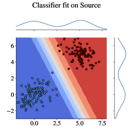
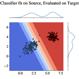
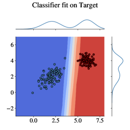
Figure 3: Illustration on how the distributional shift on features $X=[X_{1},X_{2}]$ harms classification performance. Alongside each scatter plot, we show the density $P(X_{i})$ on the side of each axis. As a consequence of distributional shift, classifiers learned with source data are ill-fitted for the target domain.

2.3 Measuring Distributional Shift

Figure 4: MSDA-based CDFD pipeline. Red arrows indicate source domain data, whereas blue arrows indicate target domain data. The CDFD model uses labeled samples from the source domains, and unlabeled data from the target domain for training a ML model adapted to the target domain.

An important question in domain adaptation is measuring the difference of $P_{S}$ and $P_{T}$ through samples $\mathbf{x}_{i}^{(P_{S})}$ and $\mathbf{x}_{j}^{(P_{T})}$. A possible approach consists on approximating $P_{S}$ (resp. $\hat{P}_{T}$) empirically, namely,

$$\hat{P}_{S}(\mathbf{x})=\dfrac{1}{n}\sum_{i=1}^{n}\delta(\mathbf{x}-\mathbf{x}_{i}^{(P_{S})}),$$ (4)

where $\delta$ is the Dirac delta. In this paper, we investigate 3 notions of distance between probability distributions, namely: (i) the $\mathcal{H}-$distance (Ben-David et al., 2010); (ii) the Maximum Mean Discrepancy (MMD) (Gretton et al., 2007); (iii) the Wasserstein distance (Villani, 2009). We now describe the empirical estimation of each of these distances.

Given $h_{d}\in\mathcal{H}$, let $n=n_{S}+n_{T}$, $\mathbf{X}=[\mathbf{X}^{(P_{S})},\mathbf{X}^{(P_{T})}]\in\mathbb{R}^{n\times n_{f}}$ and $\mathbf{d}=\{d_{i}\}_{i=1}^{n}$, where $d_{i}=0$, $i=1,\cdots,n_{S}$ and $d_{i}=1$, $i=n_{S},\cdots,n_{S}+n_{T}$. Thus, the $d_{\mathcal{H}}$ (Ben-David et al., 2010) is given by,

$$d_{\mathcal{H}}(\hat{P}_{S},\hat{P}_{T})=2\biggr{(}1-\underset{h_{d}\in\mathcal{H}}{\text{min}}\,\,\dfrac{1}{n}\sum_{i=1}^{n}\mathcal{L}(h_{d}(\mathbf{x}_{i}),d_{i})\biggr{)},$$ (5)

where $\mathcal{L}$ is commonly taken as the Binary Cross Entropy (BCE), $\mathcal{L}(\hat{d},d)=d\log\hat{d}+(1-d)\log(1-\hat{d})$. Intuitively, $d_{\mathcal{H}}$ is high if there is a classifier that can distinguish between samples from both domains.

Let $\mathcal{H}_{k}$ be a Reproducing Kernel Hilbert Space (RKHS) with kernel $k$. The MMD can be estimated using matrices $\mathbf{K}\in\mathbb{R}^{n\times n}$ and $\mathbf{L}\in\mathbb{R}^{n\times n}$ defined as,

$$\mathbf{K}=\begin{bmatrix}\mathbf{K}_{SS}&\mathbf{K}_{ST}\\ \mathbf{K}_{TS}&\mathbf{K}_{TT}\end{bmatrix}, \mathbf{L}=\begin{bmatrix}\nicefrac{{\mathbf{I}_{n_{S}}}}{{n_{S}^{2}}}&\nicefrac{{-2\mathbf{I}_{n_{S},n_{T}}}}{{n_{S}n_{T}}}\\ \nicefrac{{-2\mathbf{I}_{n_{T},n_{S}}}}{{n_{S}n_{T}}}&\nicefrac{{\mathbf{I}_{n_{T}}}}{{n_{T}^{2}}}\end{bmatrix}$$

where $\mathbf{I}_{n_{S},n_{T}}\in\mathbb{R}^{n_{S}\times n_{T}}$ is a rectangular matrix with $n_{S}$ rows and $n_{T}$ columns and $1$ on its diagonal. The matrix $\mathbf{K}_{SS}$ (resp. $\mathbf{K}_{ST},\mathbf{K}_{TT}$) has entries $(\mathbf{K}_{SS})_{i,j}=k(\mathbf{x}_{i}^{(P_{S})},\mathbf{x}_{j}^{(P_{S})})$, hence,

$$\text{MMD}(\hat{P}_{S},\hat{P}_{T}) =\text{Tr}(\mathbf{KL}),$$ (6)

where Tr$(\mathbf{A})$ denotes the trace of matrix $\mathbf{A}$. Intuitively, the MMD is a distance in a kernel space between the means of distributions.

Finally, the Wasserstein distance $W_{c}$ is rooted on the theory of Optimal Transport (OT) (Villani, 2009). In its modern computational treatment (Peyré and Cuturi, 2019), the OT problem can be phrased as,

$$\gamma^{\star}=\text{OT}(\mathbf{X}^{(P_{S})},\mathbf{X}^{(P_{T})})=\underset{\gamma\in\Gamma(\hat{P}_{S},\hat{P}_{T})}{\text{argmin}}\,\,\langle\gamma,\mathbf{C}\rangle_{F},$$ (7)

where $\gamma\in\mathbb{R}^{n_{S}\times n_{T}}$ is called OT plan, $\mathbf{C}\in\mathbb{R}^{n_{S}\times n_{T}}$ is the ground-cost matrix with $C_{ij}=c(\mathbf{x}_{i}^{(P_{S})},\mathbf{x}_{j}^{(P_{T})})$ for a ground-cost $c:\mathbb{R}^{d}\times\mathbb{R}^{d}$, and $\langle\cdot,\cdot\rangle_{F}$ is the Frobenius dot product. The set $\Gamma(\hat{P}_{S},\hat{P}_{T})=\{\gamma\in\mathbb{R}^{n_{S}\times n_{T}}:\sum_{i=1}^{n_{S}}\gamma_{i,j}=\nicefrac{{1}}{{n_{S}}}\text{ and }\sum_{j=1}^{n_{T}}\gamma_{i,j}=\nicefrac{{1}}{{n_{T}}}\}$. The ground-cost $c$ is a measure of distance between samples from $\hat{P}_{S}$ and $\hat{P}_{T}$. Problem 7 is a linear program, which can be solved exactly through the Simplex method Dantzig et al. (1955) or approximately through the Sinkhorn algorithm Cuturi (2013). We refer readers to Fernandes Montesuma et al. (2023b) for a review on the use of OT for ML.

These distances can be used for quantifying the intensity of distributional shift (Fernandes Montesuma et al., 2022), or in the design of DA algorithms. Indeed, both shallow (Courty et al., 2017a) and deep (Peng et al., 2019) DA methods employ these distances as a criterion of domain proximity. Theoretical results (Ben-David et al., 2010; Redko et al., 2017, 2019) indicate that, when distributions are close in any of these metrics, source domain error is close to target domain error.

3 Cross-Domain Fault Diagnosis

Table 1: Description of shallow and deep domain adaptation methods alongside the notion of distance they minimize during training.

Method	Distance	Category	Author
Single Source
TCA	MMD	Shallow	Pan et al. (2010)
OTDA	$W_{2}$	Shallow	Courty et al. (2017a)
JDOT	$W_{c}$	Shallow	Courty et al. (2017b)
MMD	MMD	Deep	Ghifary et al. (2014)
DANN	$d_{\mathcal{H}}$	Deep	Ganin et al. (2016)
DeepJDOT	$W_{c}$	Deep	Damodaran et al. (2018)
Multi-Source
M3SDA	MMD	Deep	Peng et al. (2019)
WJDOT	$W_{c}$	Shallow	Turrisi et al. (2022)
WBTreg	$W_{c}$	Shallow	Fernandes Montesuma and Mboula (2021a); Fernandes Montesuma and Mboula (2021b)
DaDiL-R/E	$W_{c}$	Shallow	Fernandes Montesuma et al. (2023a)

In this section we review SSDA (section 3.1) and MSDA (section 3.2) methods. These will be applied for CDFD in the next section, when unlabeled target domain samples are available. We assume that distributional shift is caused by the process conditions, such as its mode of operation. Figure 4 illustrates the overall modeling in MSDA-based CDFD.

We further make the distinction between shallow and deep DA methods. Shallow DA can be understood as a preprocessing step, as one seeks a transformation $T:\mathbb{R}^{n_{f}}\rightarrow\mathbb{R}^{n_{f}^{\prime}}$, where $n_{f}^{\prime}$ is the new feature size, so that source and target domain features are distributed similarly. Deep DA uses unlabeled samples from the target domain to reduce the distributional shift in the latent space by adding a domain discrepancy loss $\mathcal{L}_{d}$ to the overall objective in optimization. An overview of the covered methods is presented in table 1.

3.1 Single Source Domain Adaptation

Transfer Component Analysis (TCA) was first introduced by Pan et al. (2010), and consists in projecting data onto a subspace where the MMD between domains is minimal. An illustration of this principle is presented in Figure 5 (a). Let $\mathbf{K}$ be the kernel matrix, defined as in equation 6. TCA is based on the following optimization problem,

$$\mathbf{W}^{\star}= \underset{\mathbf{W}}{\text{minimize}} \text{Tr}(\mathbf{W}^{T}\mathbf{W})+\mu\text{Tr}(\mathbf{W}^{T}\mathbf{KLKW})$$

subject to $$\mathbf{W}^{T}\mathbf{KHKW}=\mathbf{I}_{n}$$

where $\mathbf{W}^{\star}\in\mathbb{R}^{n_{f}\times n_{f}^{\prime}}$, $\mathbf{H}=\mathbf{I}_{n}-\nicefrac{{1}}{{n}}\mathds{1}_{n}\mathds{1}_{n}^{T}$ is the centering matrix, and $\mu>0$ is the penalty coefficient. The projection matrix $\mathbf{W}^{\star}$ can be used for mapping points into $\mathbb{R}^{n_{f}^{\prime}}$, through $T(\mathbf{X})=\mathbf{K}\mathbf{W}^{\star}$.

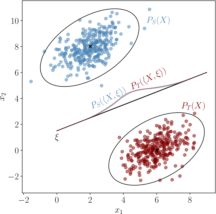
(a) Projection-based DA

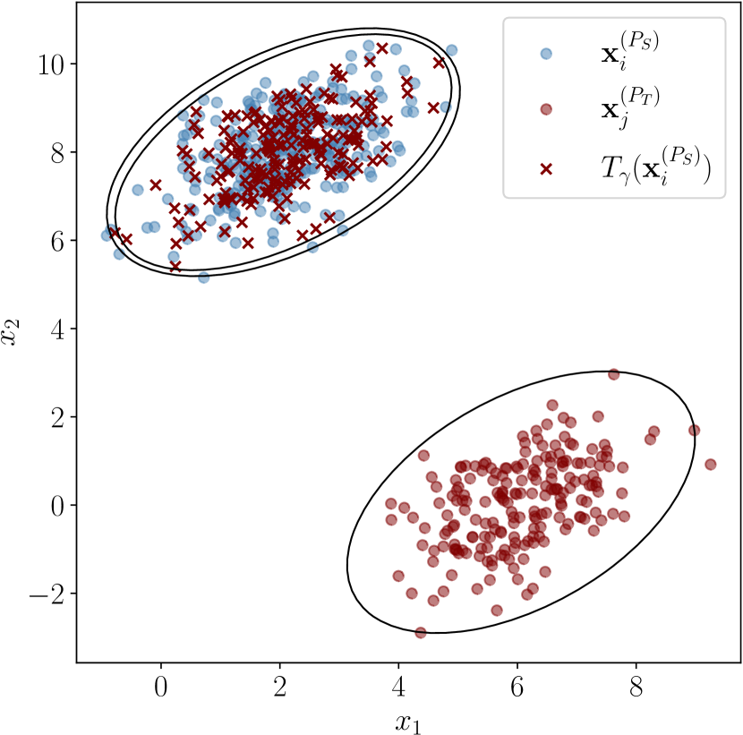
(b) OT-based DA

Figure 5: (a) $P_{S}$ and $P_{T}$ are projected over the direction $\xi$. As a consequence, the distributions $P_{S}(\langle X,\xi\rangle)$ and $P_{T}(\langle X,\xi\rangle)$. (b) Samples $\mathbf{x}_{i}^{(P_{S})}$ are transformed to be distributed according $P_{T}$ using the barycentric mapping.

Optimal Transport for Domain Adaptation (OTDA) (Courty et al., 2017a) consists on matching $\hat{P}_{S}$ and $\hat{P}_{T}$ through OT. The approach relies on the notion of barycentric mapping, defined as,

$$T_{\gamma}(\mathbf{x}_{i}^{(P_{S})})=n_{S}\gamma^{\star}\mathbf{X}^{(P_{T})},$$ (8)

where $\gamma^{\star}$ is the OT plan between $\hat{P}_{S}$ and $\hat{P}_{T}$. This strategy is shown in figure 5 (b).

Figure 6: Architecture for deep DA methods. Red and blue arrows correspond to source and target domain data respectively.

We now discuss deep DA methods. Let $\phi$ be the set of feature extraction layers in a DNN (e.g. the encoder in figure 2). We denote $\phi_{\sharp}\hat{P}$ to the pushforward distribution, resulting on the application of $\phi$ to the support of $\hat{P}$,

$$\phi_{\sharp}\hat{P}(\mathbf{z})=\dfrac{1}{n}\sum_{i=1}^{n}\delta(\mathbf{z}-\phi(\mathbf{x}_{i}^{(P)})).$$

Deep DA methods reduce the distance in distribution between $\phi_{\sharp}\hat{P}_{S}$ and $\phi_{\sharp}\hat{P}_{T}$. As such, these methods minimize,

$$\underset{\phi,h}{\text{min}}\,\,\hat{\mathcal{R}}_{S}(h\circ\phi)+\lambda\mathcal{L}_{d}(\phi,h),$$

where $\mathcal{L}_{d}$ is a domain dissimilarity loss. This idea is illustrated in figure 6.

Ghifary et al. (2014) introduced a method that relies on minimizing the MMD between features distributions,

$$\mathcal{L}_{d}(\phi)=\text{MMD}(\phi_{\sharp}\hat{P}_{S},\phi_{\sharp}\hat{P}_{T}).$$

henceforth we refer to this method as MMD.

Domain Adversarial Neural Net (DANN) was proposed by Ganin et al. (2016), and relies on the $\mathcal{H}-$distance. The authors propose adding an additional branch $h_{d}$ to classify the domain of features, that is,

$$\mathcal{L}_{d}(\phi) =\underset{h_{d}}{\text{max}}\,\,\dfrac{1}{n_{S}+n_{T}}\sum_{n=1}^{n_{S}+n_{T}}\text{BCE}(h_{d}(\phi(\mathbf{x}_{i})),d_{i}),$$

where $d_{i}\in\{0,1\}$ denotes the domain which $\mathbf{x}_{i}$ belongs to. This method is equivalent to minimizing $d_{\mathcal{H}}(\phi_{\sharp}\hat{P}_{S},\phi_{\sharp}\hat{P}_{T})$.

We further discuss the Joint Distribution Optimal Transport (JDOT) method of Courty et al. (2017b), and its latter deep DA extension proposed by Damodaran et al. (2018). This strategy models feature-label joint distributions, but, since the target domain is not labeled, one uses the approximation,

$$\hat{P}_{T}^{h}(\mathbf{x},y) =\dfrac{1}{n_{T}}\sum_{j=1}^{n_{T}}\delta((\mathbf{x},y)-(\mathbf{x}_{i}^{(P_{T})},h(\mathbf{x}_{i}^{(P_{T})}))),$$

which serves as a proxy for $\hat{P}_{T}(\mathbf{x},\mathbf{y})$. The idea of Courty et al. (2017b) is minimizing $W_{c}(\hat{P}_{S},\hat{P}_{T}^{h})$ with ground cost,

$$C_{ij} =\alpha\lVert\mathbf{x}_{i}^{(P_{S})}-\mathbf{x}_{j}^{(P_{T})}\rVert_{2}^{2}+\beta\mathcal{L}_{c}(y_{i}^{(P_{S})},h(\mathbf{x}_{j}^{(P_{T})})).$$ (9)

The JDOT strategy thus minimizes,

$$\underset{h\in\mathcal{H},\gamma\in\Gamma(\hat{P}_{S},\hat{P}_{T}^{h})}{\text{min}}\,\,\sum_{i=1}^{n_{S}}\sum_{j=1}^{n_{T}}\gamma_{ij}C_{ij}=\underset{h\in\mathcal{H}}{\text{min}}\,\,W_{c}(\hat{P}_{S},\hat{P}_{T}^{h}),$$

by alternating the minimization over $h$ and $\gamma$. As follows, Damodaran et al. (2018) extended the JDOT framework for deep DA, by using

$$\mathcal{L}_{d}(\phi) =\underset{\gamma\in\Gamma(\hat{P}_{S},\hat{P}_{T}),h}{\text{min}}\,\,\sum_{i=1}^{n_{S}}\sum_{j=1}^{n_{T}}\gamma_{i,j}C_{i,j}(\phi,h),$$

as domain dissimilarity.

3.2 Multi-Source Domain Adaptation

As shown in table 1, 4 methods fall into the multi-source category. We have 3 shallow methods, such as (i) Wasserstein Barycenter Transport (WBT), (ii) Dataset Dictionary Learning (DaDiL), and (iii) weighted JDOT and one deep method, (iv) Moment Matching for MSDA (M3SDA). In MSDA, one has various source distributions, namely $\mathcal{P}=\{\hat{P}_{S_{\ell}}\}_{\ell=1}^{N}$ and a single target $\hat{P}_{T}$.

Figure 7: Illustration of WBT, where one calculates the Wasserstein barycenter (square) of labeled distributions, then transports it to an unlabeled target domain.

WBT, proposed by Fernandes Montesuma and Mboula (2021a); Fernandes Montesuma and Mboula (2021b), is a method that relies on the Wasserstein barycenter for aggregating source distributions before transferring to target. Therefore, the authors propose solving,

$$\mathcal{B}(\alpha;\mathcal{P}) =\underset{\begin{subarray}{c}\mathbf{x}^{(B)}_{1},\cdots,\mathbf{x}^{(B)}_{j},\cdots,\mathbf{x}^{(B)}_{n}\in\mathbb{R}^{d}\\ \mathbf{y}^{(B)}_{1},\cdots,\mathbf{y}^{(B)}_{j},\cdots,\mathbf{y}^{(B)}_{n}\in\mathbb{R}^{d}\end{subarray}}{\text{argmin}}\,\,\sum_{\ell=1}^{N}\alpha_{\ell}\langle\gamma^{(\ell)},\mathbf{C}^{(\ell)}\rangle_{F},$$ (10)

$$C_{ij}^{(k)} =\lVert\mathbf{x}_{i}^{(P_{S_{\ell}})}-\mathbf{x}_{j}^{(B)}\rVert_{2}^{2}+\beta\delta(\mathbf{y}_{i}^{(P_{S_{\ell}})}-\mathbf{y}_{j}^{(B)}),$$ (11)

for $\alpha_{k}=\nicefrac{{1}}{{N}}$, and $\beta>0$ corresponding to how costly it is to transport points from different classes. This minimization problem is carried out by iterating,

$$\mathbf{X}^{(B)}_{it+1}=\sum_{\ell=1}^{N}\alpha_{\ell}T_{\gamma^{(\ell)}}(\mathbf{X}^{(B)}_{it}),\text{ and }\mathbf{Y}^{(B)}_{it+1}=\sum_{\ell=1}^{N}\alpha_{\ell}T_{\gamma^{(\ell)}}(\mathbf{Y}^{(B)}_{it}),$$

until convergence. For DA, the empirical distribution $\hat{B}$ with support $\{(\mathbf{x}_{i}^{(B)},\mathbf{y}^{(B)}_{i})\}_{i=1}^{n_{B}}$ represents an intermediate domain. As follows, Fernandes Montesuma and Mboula (2021a); Fernandes Montesuma and Mboula (2021b) employ an additional step for transporting $\hat{B}$ towards $\hat{P}_{T}$, through the barycentric mapping, i.e. $T_{\gamma}(\mathbf{X}^{(B)})$ (see equation 8).

DaDiL was proposed by Fernandes Montesuma et al. (2023a), and consists on learning a dictionary over source domain distributions. The dictionary is a pair $(\mathcal{Q},\mathcal{A})$, of a set of atoms $\mathcal{Q}=\{\hat{Q}_{k}\}_{k=1}^{K}$ and weights $\mathcal{A}=\{\alpha_{\ell}\}_{\ell=1}^{N+1}$, where $\alpha_{\ell}$ are the barycentric coordinates of $\hat{P}_{\ell}$ w.r.t. $\mathcal{Q}$. By convention, the authors use $\alpha_{N+1}=\alpha_{T}$.

Each atom is parametrized by its support, that is, $\hat{Q}_{k}=\dfrac{1}{n}\sum_{i=1}^{n}\delta_{(\mathbf{x}_{i}^{(Q_{k})},\mathbf{y}_{i}^{(Q_{k})})}$. The dictionary learning setting consists on a minimization problem,

$$(\mathcal{Q}^{\star},\mathcal{A}^{\star})=\underset{\mathcal{Q},\mathcal{A}\in\Delta_{K}^{N+1}}{\text{argmin}}\,\,\dfrac{1}{N+1}\sum_{\ell=1}^{N+1}W_{c}(\hat{P}_{\ell},\mathcal{B}(\alpha_{\ell};\mathcal{Q})),$$

where $W_{c}$ is the Wasserstein distance with,

$$C_{ij} =\lVert\mathbf{x}_{i}^{(P)}-\mathbf{x}_{j}^{(Q)}\rVert_{2}^{2}+\beta\lVert\mathbf{y}_{i}^{(P)}-\mathbf{y}_{j}^{(Q)}\rVert^{2},$$

Since the target $\hat{P}_{T}$ is not labeled, one cannot compute $W_{c}(\hat{P}_{T},\hat{B}_{T})$ directly. We use OT for pseudo-labeling the target domain, that is,

$$\hat{\mathbf{Y}}^{(P_{T})}=\dfrac{1}{N_{S}}\sum_{\ell=1}^{N_{S}}n_{\ell}(\pi_{\ell})^{T}\mathbf{Y}^{(P_{\ell})},$$

where $\pi_{\ell}=\text{OT}(\mathbf{X}^{(P_{\ell})},\mathbf{X}^{(P_{T})})$. We illustrate the overall idea behind DaDiL in figure 8.

Figure 8: Illustration of DaDiL, using the same symbols as in figure 7. In this case, each domain $\hat{P}_{\ell}$ is expressed as a barycenter in Wasserstein space of distributions $\mathcal{Q}$. In this sense, DaDiL interpolates the distributional shift of real distributions $\mathcal{P}$ through Wasserstein barycenters of $\mathcal{Q}$.

Once the dictionary is learned, the authors propose two methods for MSDA. The first, called DaDiL-R, is based on the reconstruction $\hat{B}_{T}=\mathcal{B}(\alpha_{T};\mathcal{Q})$:

$$\mathbf{X}^{(B_{T})}=\sum_{k=1}^{K}\alpha_{k}T_{\gamma^{(k)}}(\mathbf{X}^{(Q_{k})})\text{, }\mathbf{Y}^{(B_{T})}=\sum_{k=1}^{K}\alpha_{k}T_{\gamma^{(k)}}(\mathbf{Y}^{(Q_{k})}),\\$$

which allows to reconstruct labeled samples in a distribution close to $\hat{P}_{T}$. The second method, called DaDiL-E, exploits the fact that each $\hat{Q}_{k}$ is labeled, for learning an atomic classifier, i.e. $\hat{h}_{k}=\text{argmin}_{h\in\mathcal{H}}\hat{\mathcal{R}}_{Q_{k}}(h)$. For predicting samples on $\hat{P}_{T}$, DaDiL-E weights the predictions of the various atomic classifiers, i.e.,

$$\hat{h}_{\alpha_{T}}(\mathbf{x}_{j}^{(P_{T})})=\sum_{k=1}^{K}\alpha_{T,k}\hat{h}_{k}(\mathbf{x}_{j}^{(P_{T})}).$$

The intuition for this method is twofold. First, if $\hat{Q}_{k}$ is close in distribution to $\hat{P}_{T}$, it is likely to yield a good predictor for the target domain. Second, the close $\hat{Q}_{k}$ and $\hat{P}_{T}$ are, the higher will be the weights $\alpha_{T,k}$, so its predictions become more important.

M3SDA, proposed by Peng et al. (2019), employs an architecture based on a shared encoder $\phi$, and $N$ domain-specific classifiers, i.e, $\{h_{k}\}_{n=1}^{N}$. Their architecture couples the ERM procedure with a regularization term based on the moments of domains $k=1,\cdots,N$,

$$\mathcal{L}_{d}(\phi) =\Omega_{S}(\phi)+\Omega_{T}(\phi),$$

$$\Omega_{S}(\phi) =\dfrac{1}{N}\sum_{p=1}^{2}\sum_{i=1}^{N}\lVert\mu_{S_{i}}^{p}-\mu_{T}^{p}\rVert_{2},$$

$$\Omega_{T}(\phi) =\binom{N}{2}\sum_{p=1}^{2}\sum_{i=1}^{N-1}\sum_{j=i+1}^{N}\lVert\mu_{S_{i}}^{p}-\mu_{S_{j}}^{p}\rVert_{2}.$$

Figure 9: M3SDA architecture, which includes an encoder $\phi$, and domain-specific classifiers $h_{i}$. For M3SDA-$\beta$, each $h_{i}$ is paired with $h_{i}^{\prime}$ which is trained for minimizing the prediction discrepancy on target domain data.

where $\mu_{S_{i}}^{p}=\mathbb{E}_{\mathbf{x}\sim P_{S_{i}}}[\phi(\mathbf{x})^{p}]$ corresponds to the entry-wise power of the mean vector on the $i-$th source (resp. target). This is similar to a MMD distance between sources $i$ and $j$, and each source and the target, for a polynomial kernel. The M3SDA algorithm is based on the optimization problem,

$$\underset{\phi,\{h_{k}\}_{k=1}^{N}}{\text{min}}\,\,\dfrac{1}{N}\sum_{k=1}^{N}\hat{\mathcal{R}}_{S_{\ell}}(h_{k}\circ\phi)+\Omega(\phi).$$ (12)

Peng et al. (2019) further proposes M3SDA-$\beta$, which employs pairs of classifiers $\{(h_{k},h_{k}^{\prime})\}_{k=1}^{K}$. Besides minimizing 12, they add other 2 learning phases. First,

$$\underset{h^{\prime}_{k}}{\text{min}}\,\,\sum_{k=1}^{N}\hat{\mathcal{R}}_{S_{\ell}}(h_{k}^{\prime}\circ\phi)-\sum_{k=1}^{N}\sum_{j=1}^{n_{T}}|h_{k}(\mathbf{z}_{j}^{(P_{T})})-h_{k}^{\prime}(\mathbf{z}_{j}^{(P_{T})})|,$$

where the second term denotes the output discrepancy on the target domain of $(h_{k},h_{k}^{\prime})$. Second,

$$\underset{\phi}{\text{min}}\,\,\sum_{k=1}^{N}\sum_{j=1}^{n_{T}}|h_{k}(\phi(\mathbf{x}_{j}^{(P_{T})}))-h_{k}^{\prime}(\phi(\mathbf{x}_{j}^{(P_{T})}))|.$$

Thus, MSDA-$\beta$ consists on alternating between the three training steps at each iteration. For generating the final predictions on the target domain, Peng et al. (2019) proposes weighting the domain-specific classifiers predictions, i.e.,

$$\hat{y}^{(P_{T})}=\sum_{k=1}^{N}w_{k}h_{k}(\mathbf{x}^{(P_{T})}),$$

for $w_{k}=acc_{k}/\sum_{\ell=1}^{N}acc_{\ell}$, where $acc_{k}$ denotes the classification accuracy of $h_{k}$ on its respective domain. The overall architecture of these 2 methods is shown in figure 9.

Weighted JDOT (WJDOT), proposed by Turrisi et al. (2022), adapts the JDOT framework for MSDA. Given $\alpha\in\Delta_{N}$, the authors aggregate $\{\hat{P}_{S_{\ell}}\}_{k=1}^{N}$ linearly, namely,

$$\hat{P}_{\alpha} =\sum_{k=1}^{N}\alpha_{k}\hat{P}_{k}=\sum_{k=1}^{N}\dfrac{\alpha_{k}}{n_{S_{\ell}}}\sum_{i=1}^{n_{S_{\ell}}}\delta_{(\mathbf{x}^{(P_{S_{\ell}})},y^{(P_{S_{\ell}})})},$$

that is, $\hat{P}_{\alpha}$ is a distribution with $n=\sum_{k}n_{S_{\ell}}$ samples, with different importance (i.e. $\alpha_{k}/n_{S_{\ell}}$). WJDOT then minimizes,

$$\underset{\alpha\in\Delta,h\in\mathcal{H}}{\text{argmin}}\,\,W_{c}(\hat{P}_{\alpha},\hat{P}_{T}^{h}),$$

which is carried, as in JDOT, by alternating between minimizing $\alpha$ for fixed $h\in\mathcal{H}$ and vice-versa.

4 Case Study

The TE process is a benchmark introduced by Downs and Vogel (1993), and is based on an actual industrial process. As such, it is a large-scale non-linear model of a complex multi-component system. Following its original description, the process produces two products from four reactants, as well as an inert and a byproduct. In total, one has eight components: $A,B,\cdots,H$, whose reactions are,

$$A(\text{g})+C(\text{g})+D(\text{g}) \rightarrow G(\text{liq})$$ Product 1,

$$A(\text{g})+C(\text{g})+E(\text{g}) \rightarrow H(\text{liq})$$ Product 2,

$$A(\text{g})+E(\text{g}) \rightarrow F(\text{liq})$$ Byproduct,

$$3D(\text{g}) \rightarrow 2F(\text{liq})$$ Byproduct.

These four reactions are irreversible and exothermic. Overall, the TE process has five major unit operations: the reactor, the product condenser, a vapor-liquid separator, a recycle compressor, and a product stripper. From these different components, $53$ process variables are measured or manipulated, as shown in table 2. We refer to Downs and Vogel (1993) for further details on the functioning of the TE process.

4.1 Process Variables and Faults

Table 2: Description of process variables of the TE process. We mark used variables in bold.

Variable	Description	Variable	Description
XME(1)	A Feed (kscmh)	XME(29)	Component A in Purge (mol %)
XME(2)	D Feed (kg/h)	XME(30)	Component B in Purge (mol %)
XME(3)	E Feed (kg/h)	XME(31)	Component C in Purge (mol %)
XME(4)	A & C Feed (kg/h)	XME(32)	Component D in Purge (mol %)
XME(5)	Recycle Flow (kscmh)	XME(33)	Component E in Purge (mol %)
XME(6)	Reactor Feed rate (kscmh)	XME(34)	Component F in Purge (mol %)
XME(7)	Reactor Pressure (kscmh)	XME(35)	Component G in Purge (mol %)
XME(8)	Reactor Level (%)	XME(36)	Component H in Purge (mol %)
XME(9)	Reactor Temperature (°C)	XME(37)	Component D in Product (mol %)
XME(10)	Purge Rate (kscmh)	XME(38)	Component E in Product (mol %)
XME(11)	Product Sep Temp (°C)	XME(39)	Component F in Product (mol %)
XME(12)	Product Sep Level (%)	XME(40)	Component G in Product (mol %)
XME(13)	Product Sep Pressure (kPa gauge)	XME(41)	Component H in Product (mol %)
XME(14)	Product Sep Underflow (m3/h)	XMV(1)	D Feed (%)
XME(15)	Stripper Level (%)	XMV(2)	E Feed (%)
XME(16)	Stripper Pressure (kPa gauge)	XMV(3)	A Feed (%)
XME(17)	Stripper Underflow (m3/h)	XMV(4)	A & C Feed (%)
XME(18)	Stripper Temp (°C)	XMV(5)	Compressor recycle valve (%)
XME(19)	Stripper Steam Flow (kg/h)	XMV(6)	Purge valve (%)
XME(20)	Compressor Work (kW)	XMV(7)	Separator liquid flow (%)
XME(21)	Reactor Coolant Temp (°C)	XMV(8)	Stripper liquid flow (%)
XME(22)	Separator Coolant Temp (°C)	XMV(9)	Stripper steam valve (%)
XME(23)	Component A to Reactor (mol %)	XMV(10)	Reactor coolant (%)
XME(24)	Component B to Reactor (mol %)	XMV(11)	Condenser Coolant (%)
XME(25)	Component C to Reactor (mol %)	XMV(12)	Agitator Speed (%)
XME(26)	Component D to Reactor (mol %)
XME(27)	Component E to Reactor (mol %)
XME(28)	Component F to Reactor (mol %)

The TE process contains a $53$ variables, divided into measured (XME), and manipulated (XMV). Table 2 presents each variable alongside its description. Henceforth we proceed as Reinartz et al. (2021) and consider the continuous process measurements and manipulated variables for fault diagnosis, i.e., XME(1) through XME(22) and XMV(1) through XMV(12). As a consequence we have multi-variate time series with $n_{f}=34$ dimensions. We further detail the pre-processing of measurements in section 4.3.

Alongside the process variables, Downs and Vogel (1993) introduced $20$ types of process disturbance, here treated as faults, with the purpose of testing control strategies (faults 1 through 20). This set was further extended by Bathelt et al. (2015), who added faults 21 through 28. In total, there are $28$ faults, which are shown in table 3. Therefore, we consider a wider set of faults than previous works (Wu and Zhao, 2020). Fault diagnosis over the TE process corresponds to a classification problem with $n_{c}=29$ classes. We refer readers to Russell et al. (2000) for more information about these faults.

Table 3: Description and types of faults for the TE process in the simulation environment of Reinartz et al. (2021).

Fault Class	Variable	Type
1	A/C feed ratio, B composition constant	Step
2	B composition, A/C ratio constant	Step
3	D feed temperature	Step
4	Water inlet temperature (reactor)	Step
5	Water inlet temperature (condenser)	Step
6	A feed loss	Step
7	C header pressure loss	Step
8	A/B/C composition of stream 4	Random Variation
9	D feed temperature 4	Random Variation
10	C feed temperature	Random Variation
11	Water outlet temperature (reactor)	Random Variation
12	Water outlet temperature (separator)	Random Variation
13	Reaction kinetics	Random Variation
14	Water outlet temperature (reactor)	Sticking
15	Water outlet temperature (separator)	Sticking
16	Variation coefficient of the steam supply of the heat exchange of the stripper	Random variation
17	Variation coefficient of heat transfer (reactor)	Random variation
18	Variation coefficient of heat transfer (condenser)	Random variation
19	Unknown	Unknown
20	Unknown	Random variation
21	A feed temperature	Random variation
22	E feed temperature	Random variation
23	A feed flow	Random variation
24	D feed flow	Random variation
25	E feed flow	Random variation
26	A & C feed flow	Random variation
27	Water flow (reactor)	Random variation
28	Water flow (condenser)	Random variation

4.2 Cross-Domain Fault Diagnosis Setting

Table 4: TE process operation modes, as described in Downs and Vogel (1993).

Mode	$G/H$ Mass Ratio	Production rate
1	50/50	7038 kg h-1 G and 7038 kg h-1 H
2	10/90	1408 kg h-1 G and 12,669 kg h-1 H
3	90/10	10,000 kg h-1 G and 1111 kg h-1 H
4	50/50	maximum production rate
5	10/90	maximum production rate
6	90/10	maximum production rate

As discussed by Downs and Vogel (1993), the TE process has 6 modes of operation, corresponding to three different $G/H$ mass ratios. These are shown in table 4. Each of these modes of operation determine different system dynamics. As studied by Ricker (1995), each of them has an specific associated steady-state. As a consequence, the statistical properties of sensor readings may drastically change between two given modes of operation, making the diagnosis task more challenging. This remark motivates the CDFD setting, and is illustrated in figure 10(a).

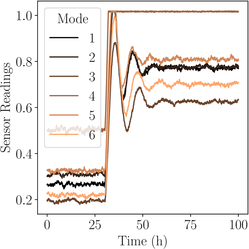
(a) Readings under different modes of operation.

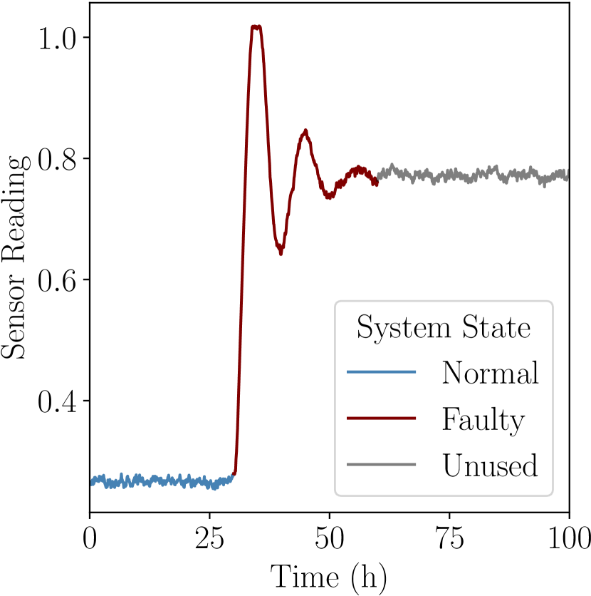
(b) Cropping the signal into normal and faulty.

Figure 10: Visualization how the modes of operation impact sensor readings (a), and how a signal is segmented into normal and faulty operation (b).

4.3 Data Acquisition and Pre-processing

We use the data made available by Reinartz et al. (2021). The dataset published by the authors contain a wide variety of simulations, which encompass single fault, set-point variation and mode transitions. We consider only the single-fault scenario.

Within the single-fault simulation group, Reinartz et al. (2021) simulated each mode of operation and each fault $100$ times, which makes a total of $17400$ simulations. Nonetheless, some of these simulations do not complete. In this case we exclude the simulation from our pre-processed dataset. This results in a total of $17289$ samples, and a slightly imbalanced dataset.

For each sample in the dataset of Reinartz et al. (2021), we segment the signal into 3 parts, consisting on $30$ hours of normal operation, the subsequent $30$ hours of faulty operation, and the remaining 40 hours of unused readings. This is shown in Figure 10(b). Hence, we have multivariate time series of shape $(34,600)$, where $34$ consists on the number of variables (see section 4.1) and $600$ to the number of time steps. Finally, for having a balanced fault dataset, we sub-sample the normal operation class so as to have $100$ samples as the other classes. We further standardize each variable independently, i.e.,

$$\mathbf{x}_{i}=\dfrac{\mathbf{x}_{i}-\mu_{i}}{\sigma_{i}}\text{, }i=1,\cdots,n_{f},$$

for the temporal mean $\mu_{i}=T^{-1}\sum_{t=1}^{T}x_{i,t}$, and variance $\sigma_{i}=(T(T-1))^{-1}\sum_{t=1}^{T}(x_{i,t}-\mu_{i})^{2}$.

5 Experiments

In what follows, we divide our experiments in terms of SSDA and MSDA. In the first case, classifiers only have access to training data coming from a single source domain. In the second case, data comes from $5$ source domains, i.e., all modes of operation except the target. Our goal is verifying whether MSDA improves performance on the target domain w.r.t. baselines and SSDA strategies.

Neural Network Architecture. Our experiments involve training a CNN from scratch. For deep DA methods, training is done by minimizing the cross-entropy loss and the distance in probability between sources and target domain. For shallow DA, the CNN is pre-trained on the concatenation of source domain data, then adaptation is performed using the convolutional layers as a feature extractor. We employ a Fully Convolutional Network (FCN) (Long et al., 2015; Wang et al., 2017; Ismail Fawaz et al., 2019), which consists on three convolutional blocks followed by a Global Average Pooling (GAP) layer. Each convolutional block has a convolutional layer, and a normalization layer. In our experiments we verified that instance normalization (Ulyanov et al., 2016) improves stability and performance over other normalization layers such as batch normalization (Ioffe and Szegedy, 2015).

5.1 Single-Source CDFD

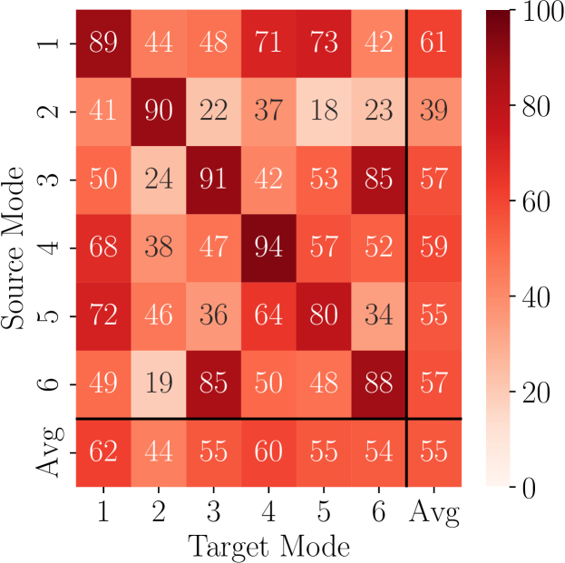
Figure 11: Baseline cases for single-source domain adaptation. Each cell $(i,j)$ corresponds to the adaptation from a labeled source mode $i$, to an unlabeled target mode $j$. The diagonal is filled with the target-only scenario, in which no distributional shift is present.

As a first candidate solution, we explore single-source DA for the TE process data. This scenario will help us illustrate the benefits of employing multi-source DA. We compare the 6 algorithms discussed in section 3.1, and listed in table 1 with two baselines.

Baselines. For single-source DA, we explore two baselines. The first, named source-only, do not use any data from the target domain during training. The second, named target-only, corresponds to learning a classifier with labeled target domain data. These approaches can be loosely associated with the worst and best case scenarios respectively. Indeed, for the source-only baseline, one applies a classifier that is ill-fitted for the target domain, as in figure 3. For the target-only baseline, no adaptation is needed, as both train and test data come from the same distribution. These remarks are validated in figure 11, which show that, for each domain, the source-only baseline (off-diagonal values) is inferior to the target-only scenario (diagonal values). As we discuss in the upcoming sections, this is also true for SSDA, but MSDA manages to improve over the target-only baseline.

On the one hand, adaptation from and towards mode 2 is more difficult than other modes. Nonetheless, when no shift is present it still achieves $90\%$ classification accuracy. These remarks indicate that this mode is more different in distribution than the others. On the other hand, the pair of modes $(3,6)$ has the highest classification accuracy, namely, $85\%$. This is close to the no-shift scenario, i.e. $91\%$ and $88\%$ for modes 3 and 6 respectively. This indicates that these domains share common characteristics.

Single-Source CDFD. In this setting, adaptation is done between pairs of modes $(S_{i},T_{j})$, with $S_{i}\neq T_{j}$. During training, DA algorithms have access to labeled data from $S_{i}$, and unlabeled data from $T_{j}$. Figure 12 shows a summary of our experiments. Overall, OT-based methods perform better than others (e.g., TCA and DANN). This remark agrees with previous research (Fernandes Montesuma et al., 2022) on CDFD.

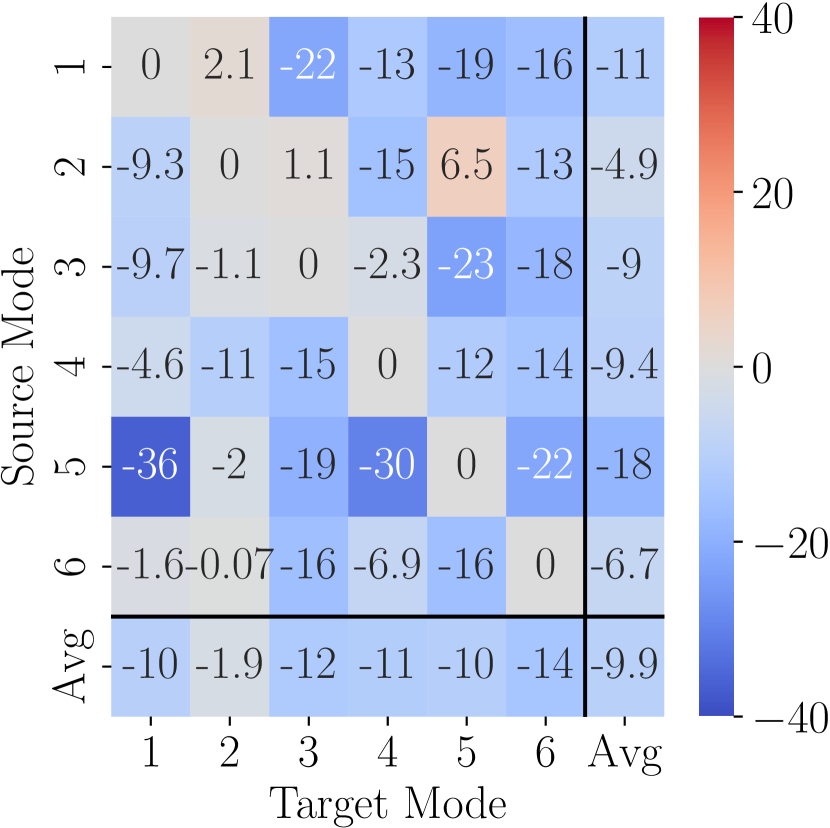
(a) DANN

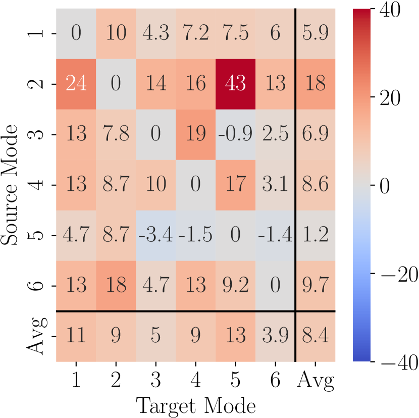
(b) OTDA

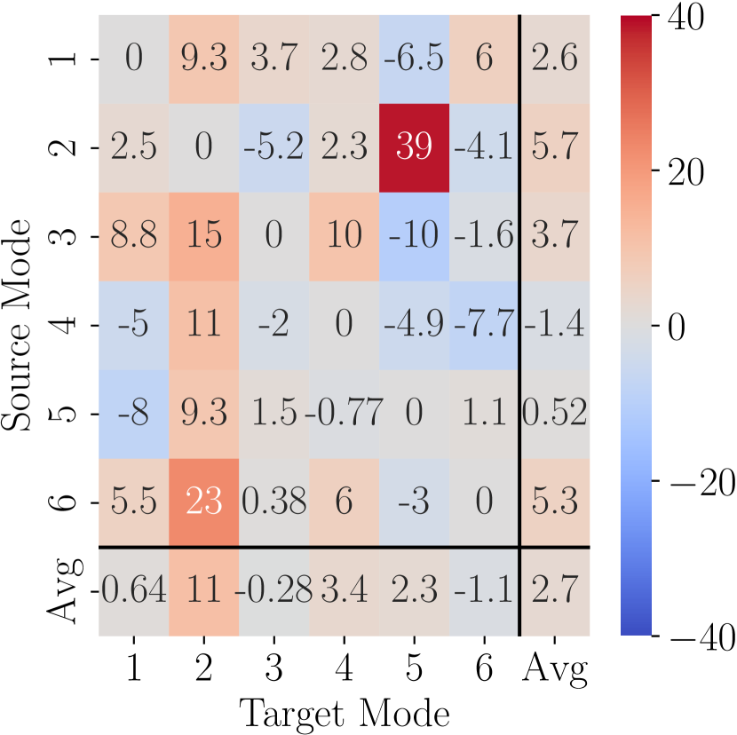
(c) MMD

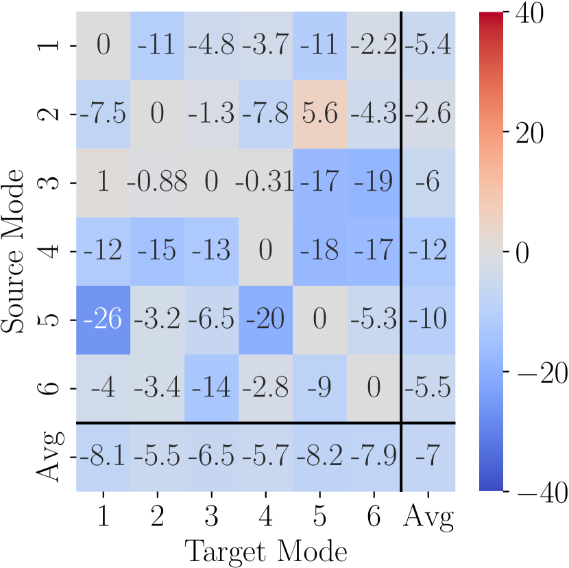
(d) TCA

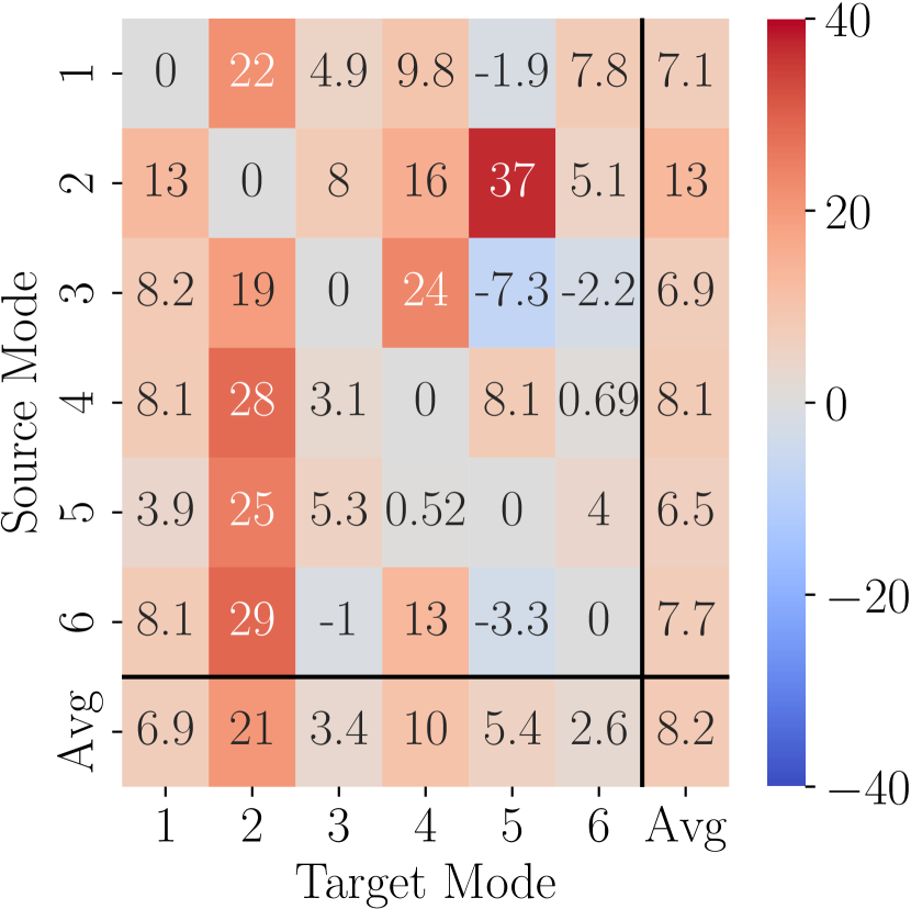
(e) DeepJDOT

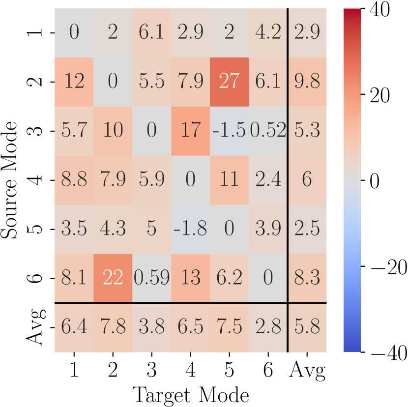
(f) JDOT

Figure 12: Performance variation with respect to baseline for single-source domain adaptation methods.

5.2 Multi-Source CDFD

In this section we explore MSDA for CDFD. We compare all methods (single, and multi-source) described in section 3. Here, SSDA methods have access to data from multiple domains, but these domains are treated as a single homogeneous domain.

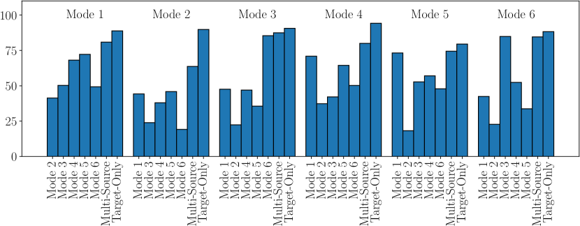
Figure 13: Comparison between single-source, multi-source and target-only baselines.

Baselines. As before, we compare all methods to source and target-only baselines. For the source-only baseline, we assume access to labeled data coming from $5$ given modes (all modes except the target). Thus, the MSDA baseline has access to a larger quantity and diversity of data, which improves performance as shown in figure 13.

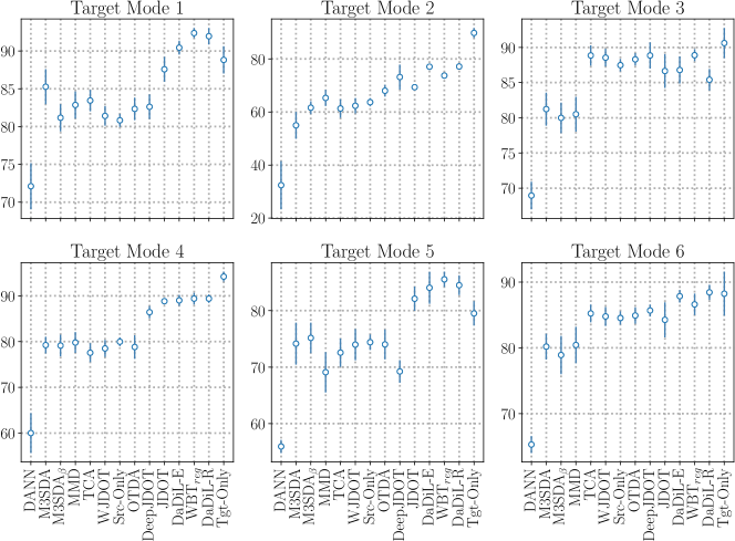
Figure 14: Comparison of adaptation performance of DA algorithms in the multi-source setting, for each mode of operation.

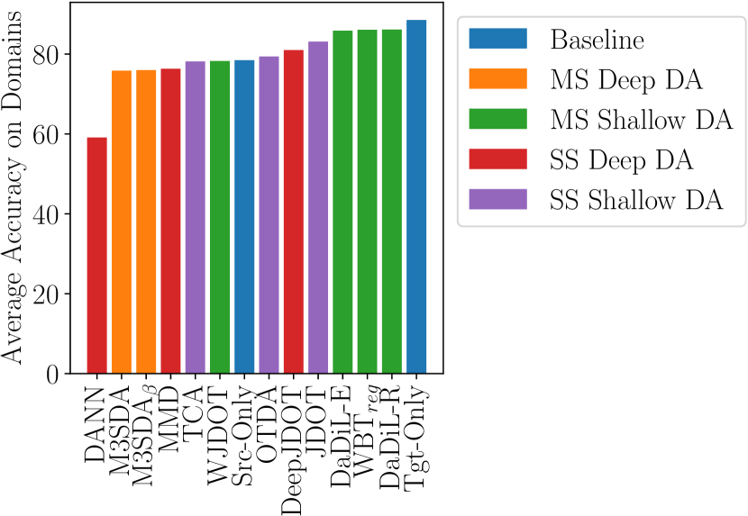
Figure 15: Comparison of average adaptation performance of DA algorithms in the multi-source setting.

Multi-Source CDFD. In this setting, in addition to labeled data from all source domains, algorithms have access to unlabeled data from the target domain. We show our results in figure 14. In overall, MSDA is able to improve over the target-only baseline for modes 1 and 5. In mode 6, MSDA and the target-only baseline are equivalent. In mode 3, SSDA algorithms improve over MSDA. Indeed, this mode has a closely related mode, i.e. mode 6.

Finally, figure 15 shows a comparison of DA algorithms in terms of their average classification accuracy over all domains. We highlight 3 remarks. First, shallow DA outperforms deep DA. Indeed, when an effective feature extractor can be trained using source domain data, transforming the data so as to minimize distributional shift is easier than learning an encoder that mitigates distributional shift. Second, the only methods that improve over the source-only baseline are OT-based techniques. Third, Wasserstein barycenter-based techniques, such as DaDiL and WBT outperforms other methods. These remarks agree with previous works in DA (Courty et al., 2017a; Fernandes Montesuma et al., 2023a), and CDFD (Fernandes Montesuma et al., 2022), and show the power of OT as a framework for both SSDA and MSDA.

6 Conclusion

In this paper, we propose multi-source unsupervised domain adaptation as a candidate solution for cross-domain fault diagnosis of chemical processes. We present a comprehensive comparison of state-of-the-art SSDA and MSDA methods in the context of the TE process (Downs and Vogel, 1993; Reinartz et al., 2021), a widely used large-scale chemical process.

In the single-source setting, we show that DA methods are able to improve the CNN baseline by 8.4% at best. Even though some pairs of modes of operation are closely related, i.e. $(1,5)$ , $(1,4)$ and $(3,6)$, SSDA is on average harder than MSDA, since one does not know a priori which modes of operation will transfer appropriately. Overall, OT-based approaches, such as OTDA (Courty et al., 2017a) or JDOT (Courty et al., 2017b) have the best performance, which agrees with previous studies in single-source CDFD (Fernandes Montesuma et al., 2022).

In the multi-source setting, the baseline improves over 23.48% on average w.r.t. the single-source. This increase is mainly due a larger quantity and diversity of data in the training set. The best SSDA method, JDOT (Courty et al., 2017b) in the MSDA setting, has an average performance of 83.13%, while the best MSDA method, DaDiL of Fernandes Montesuma et al. (2023a), has an average performance of 86.14%. Thus, the larger amount of data improves over SSDA, and considering data heterogeneity further improves performance.

We hope that the present work will encourage future research on MSDA for CDFD. Future works include evaluating the statistical challenges of estimating distributional shift when data is high dimensional. Furthermore, exploring the robustness of methods w.r.t. class imbalance is key, as in many cases, non-faulty samples are more frequent. Finally, exploring DA between simulated and real data is an important direction for CDFD research, as previously explored in (Li et al., 2020; Fernandes Montesuma et al., 2022).

References

- Isermann [2006] Rolf Isermann. Fault-diagnosis systems: an introduction from fault detection to fault tolerance. Springer Science & Business Media, 2006.
- Vapnik [1991] Vladimir Vapnik. Principles of risk minimization for learning theory. Advances in neural information processing systems, 4, 1991.
- Quinonero-Candela et al. [2008] Joaquin Quinonero-Candela, Masashi Sugiyama, Anton Schwaighofer, and Neil D Lawrence. Dataset shift in machine learning. Mit Press, 2008.
- Zheng et al. [2019] Huailiang Zheng, Rixin Wang, Yuantao Yang, Jiancheng Yin, Yongbo Li, Yuqing Li, and Minqiang Xu. Cross-domain fault diagnosis using knowledge transfer strategy: a review. IEEE Access, 7:129260–129290, 2019.
- Peng et al. [2019] Xingchao Peng, Qinxun Bai, Xide Xia, Zijun Huang, Kate Saenko, and Bo Wang. Moment matching for multi-source domain adaptation. In Proceedings of the IEEE/CVF international conference on computer vision, pages 1406–1415, 2019.
- Blitzer et al. [2007] John Blitzer, Mark Dredze, and Fernando Pereira. Biographies, bollywood, boom-boxes and blenders: Domain adaptation for sentiment classification. In Proceedings of the 45th annual meeting of the association of computational linguistics, pages 440–447, 2007.
- Li et al. [2020] Weijun Li, Sai Gu, Xiangping Zhang, and Tao Chen. Transfer learning for process fault diagnosis: Knowledge transfer from simulation to physical processes. Computers & Chemical Engineering, page 106904, 2020.
- Fernandes Montesuma et al. [2022] Eduardo Fernandes Montesuma, Michela Mulas, Francesco Corona, and Fred-Maurice Ngole Mboula. Cross-domain fault diagnosis through optimal transport for a cstr process. IFAC-PapersOnLine, 55(7):946–951, 2022.
- Wu and Zhao [2020] Hao Wu and Jinsong Zhao. Fault detection and diagnosis based on transfer learning for multimode chemical processes. Computers & Chemical Engineering, 135:106731, 2020.
- Turrisi et al. [2022] Rosanna Turrisi, Rémi Flamary, Alain Rakotomamonjy, and Massimiliano Pontil. Multi-source domain adaptation via weighted joint distributions optimal transport. In Uncertainty in Artificial Intelligence, pages 1970–1980. PMLR, 2022.
- Fernandes Montesuma and Mboula [2021a] Eduardo Fernandes Montesuma and Fred-Maurice Ngolè Mboula. Wasserstein barycenter transport for acoustic adaptation. In ICASSP 2021-2021 IEEE International Conference on Acoustics, Speech and Signal Processing (ICASSP), pages 3405–3409. IEEE, 2021a.
- Fernandes Montesuma and Mboula [2021b] Eduardo Fernandes Montesuma and Fred Maurice Ngole Mboula. Wasserstein barycenter for multi-source domain adaptation. In Proceedings of the IEEE/CVF Conference on Computer Vision and Pattern Recognition, pages 16785–16793, 2021b.
- Fernandes Montesuma et al. [2023a] Eduardo Fernandes Montesuma, Fred Ngolè Mboula, and Antoine Souloumiac. Multi-source domain adaptation through dataset dictionary learning in wasserstein space. arXiv preprint arXiv:2307.14953, 2023a. Accepted as a conference paper in the 26th European Conference on Artificial Intelligence.
- Downs and Vogel [1993] James J Downs and Ernest F Vogel. A plant-wide industrial process control problem. Computers & chemical engineering, 17(3):245–255, 1993.
- Melo et al. [2022] Afrânio Melo, Maurício M Câmara, Nayher Clavijo, and José Carlos Pinto. Open benchmarks for assessment of process monitoring and fault diagnosis techniques: A review and critical analysis. Computers & Chemical Engineering, page 107964, 2022.
- LeCun et al. [2015] Yann LeCun, Yoshua Bengio, and Geoffrey Hinton. Deep learning. nature, 521(7553):436–444, 2015.
- Bengio et al. [2013] Yoshua Bengio, Aaron Courville, and Pascal Vincent. Representation learning: A review and new perspectives. IEEE transactions on pattern analysis and machine intelligence, 35(8):1798–1828, 2013.
- Ismail Fawaz et al. [2019] Hassan Ismail Fawaz, Germain Forestier, Jonathan Weber, Lhassane Idoumghar, and Pierre-Alain Muller. Deep learning for time series classification: a review. Data mining and knowledge discovery, 33(4):917–963, 2019.
- Pan and Yang [2009] Sinno Jialin Pan and Qiang Yang. A survey on transfer learning. IEEE Transactions on knowledge and data engineering, 22(10):1345–1359, 2009.
- Ben-David et al. [2010] Shai Ben-David, John Blitzer, Koby Crammer, Alex Kulesza, Fernando Pereira, and Jennifer Wortman Vaughan. A theory of learning from different domains. Machine learning, 79(1):151–175, 2010.
- Gretton et al. [2007] Arthur Gretton, Karsten M Borgwardt, Malte Rasch, Bernhard Schölkopf, and Alexander J Smola. A kernel approach to comparing distributions. In Proceedings of the National Conference on Artificial Intelligence, volume 22, page 1637. Menlo Park, CA; Cambridge, MA; London; AAAI Press; MIT Press; 1999, 2007.
- Villani [2009] Cédric Villani. Optimal transport: old and new, volume 338. Springer, 2009.
- Peyré and Cuturi [2019] Gabriel Peyré and Marco Cuturi. Computational optimal transport: With applications to data science. Foundations and Trends® in Machine Learning, 11(5-6):355–607, 2019.
- Dantzig et al. [1955] George B Dantzig, Alex Orden, Philip Wolfe, et al. The generalized simplex method for minimizing a linear form under linear inequality restraints. Pacific Journal of Mathematics, 5(2):183–195, 1955.
- Cuturi [2013] Marco Cuturi. Sinkhorn distances: Lightspeed computation of optimal transport. Advances in neural information processing systems, 26, 2013.
- Fernandes Montesuma et al. [2023b] Eduardo Fernandes Montesuma, Fred Ngole Mboula, and Antoine Souloumiac. Recent advances in optimal transport for machine learning. arXiv preprint arXiv:2306.16156, 2023b.
- Courty et al. [2017a] Nicolas Courty, Rémi Flamary, Devis Tuia, and Alain Rakotomamonjy. Optimal transport for domain adaptation. IEEE Transactions on Pattern Analysis and Machine Intelligence, 39(9):1853–1865, 2017a. doi:10.1109/TPAMI.2016.2615921.
- Redko et al. [2017] Ievgen Redko, Amaury Habrard, and Marc Sebban. Theoretical analysis of domain adaptation with optimal transport. In Joint European Conference on Machine Learning and Knowledge Discovery in Databases, pages 737–753. Springer, 2017.
- Redko et al. [2019] Ievgen Redko, Emilie Morvant, Amaury Habrard, Marc Sebban, and Younes Bennani. Advances in domain adaptation theory. Elsevier, 2019.
- Pan et al. [2010] Sinno Jialin Pan, Ivor W Tsang, James T Kwok, and Qiang Yang. Domain adaptation via transfer component analysis. IEEE Transactions on Neural Networks, 22(2):199–210, 2010.
- Courty et al. [2017b] Nicolas Courty, Rémi Flamary, Amaury Habrard, and Alain Rakotomamonjy. Joint distribution optimal transportation for domain adaptation. Advances in neural information processing systems, 30, 2017b.
- Ghifary et al. [2014] Muhammad Ghifary, W Bastiaan Kleijn, and Mengjie Zhang. Domain adaptive neural networks for object recognition. In Pacific Rim international conference on artificial intelligence, pages 898–904. Springer, 2014.
- Ganin et al. [2016] Yaroslav Ganin, Evgeniya Ustinova, Hana Ajakan, Pascal Germain, Hugo Larochelle, François Laviolette, Mario Marchand, and Victor Lempitsky. Domain-adversarial training of neural networks. The Journal of Machine Learning Research, 17(1):2096–2030, 2016.
- Damodaran et al. [2018] Bharath Bhushan Damodaran, Benjamin Kellenberger, Rémi Flamary, Devis Tuia, and Nicolas Courty. Deepjdot: Deep joint distribution optimal transport for unsupervised domain adaptation. In Proceedings of the European Conference on Computer Vision (ECCV), pages 447–463, 2018.
- Reinartz et al. [2021] Christopher Reinartz, Murat Kulahci, and Ole Ravn. An extended tennessee eastman simulation dataset for fault-detection and decision support systems. Computers & Chemical Engineering, 149:107281, 2021.
- Bathelt et al. [2015] Andreas Bathelt, N Lawrence Ricker, and Mohieddine Jelali. Revision of the tennessee eastman process model. IFAC-PapersOnLine, 48(8):309–314, 2015.
- Russell et al. [2000] Evan L. Russell, Leo H. Chiang, and Richard D. Braatz. Tennessee Eastman Process, pages 99–108. Springer London, London, 2000. ISBN 978-1-4471-0409-4. doi:10.1007/978-1-4471-0409-4_8. URL https://doi.org/10.1007/978-1-4471-0409-4_8.
- Ricker [1995] NL Ricker. Optimal steady-state operation of the tennessee eastman challenge process. Computers & chemical engineering, 19(9):949–959, 1995.
- Long et al. [2015] Jonathan Long, Evan Shelhamer, and Trevor Darrell. Fully convolutional networks for semantic segmentation. In Proceedings of the IEEE conference on computer vision and pattern recognition, pages 3431–3440, 2015.
- Wang et al. [2017] Zhiguang Wang, Weizhong Yan, and Tim Oates. Time series classification from scratch with deep neural networks: A strong baseline. In 2017 International joint conference on neural networks (IJCNN), pages 1578–1585. IEEE, 2017.
- Ulyanov et al. [2016] Dmitry Ulyanov, Andrea Vedaldi, and Victor Lempitsky. Instance normalization: The missing ingredient for fast stylization. arXiv preprint arXiv:1607.08022, 2016.
- Ioffe and Szegedy [2015] Sergey Ioffe and Christian Szegedy. Batch normalization: Accelerating deep network training by reducing internal covariate shift. In International conference on machine learning, pages 448–456. pmlr, 2015.