Time-reversal symmetry-breaking flux state in an organic Dirac fermion system

Abstract

We investigate symmetry breaking in the Dirac fermion phase of the organic compound $\alpha$-(BEDT-TTF)₂I₃ under pressure, where BEDT-TTF denotes bis(ethylenedithio)tetrathiafulvalene. The exchange interaction resulting from inter-molecule Coulomb repulsion leads to broken time-reversal symmetry and particle-hole symmetry, while preserving translational symmetry. The system breaks time-reversal symmetry by creating fluxes in the unit cell. This symmetry-broken state exhibits a large Nernst signal as well as thermopower. We compute the Nernst signal and thermopower, demonstrating their consistency with experimental results.

I Introduction

Organic charge-transfer salt, $\alpha$-(BEDT-TTF)₂I₃, has been extensively studied as a quasi-two-dimensional Dirac fermion system [1, 2, 3]. Here, BEDT-TTF refers to bis(ethylenedithio)tetrathiafulvalene. The extended Hubbard model, incorporating the pressure dependence in the transfer energies obtained from X-ray diffraction experiments [4, 5, 6], predicts a two-dimensional Dirac fermion spectrum with charge disproportionation under high pressures [2], a result corroborated by first principles calculations [7, 8]. The presence of the Dirac fermion spectrum is evident through the large negative interlayer magnetoresistance, attributed to the zero-energy Landau level of the Dirac fermions [9, 10]. Additionally, the phase of the Dirac fermions is confirmed through Shubnikov-de Haas oscillations in hole-doped samples placed on polyethylene naphthalate substrates [11].

Recently, research on $\alpha$-(BEDT-TTF)₂I₃ has reached a turning point with theoretical results suggesting broken time-reversal and inversion symmetry [12], and experimental findings indicating that the system exhibits characteristics of a three-dimensional Dirac semimetal at low temperatures [13]. The observation of a peak in the interlayer magnetoresistance at low temperatures indicates phase-coherent interlayer tunneling, implying a three-dimensional electronic structure [14]. Furthermore, the detection of negative magnetoresistance and the planar Hall effect provide supporting evidence for $\alpha$-(BEDT-TTF)₂I₃ being a Dirac semimetal [13], which necessitates breaking either time-reversal symmetry, inversion symmetry, or both.

In this paper, we investigate the origin of broken time-reversal symmetry and inversion symmetry in $\alpha$-(BEDT-TTF)₂I₃. We find that the symmetry breaking arises from a flux state. The unit cell of $\alpha$-(BEDT-TTF)₂I₃ contains four BEDT-TTF molecules, as depicted in Fig. 1, denoted by A, A^′, B, and C, and inversion symmetry exists between A and A^′ molecules[4, 15, 16]. We demonstrate that this inversion symmetry is broken and the exchange interaction induces asymmetry in the phases of the hopping matrix elements between A and A^′ molecules, consequently breaking time-reversal symmetry and particle-hole symmetry.

While direct verification of broken time-reversal symmetry is challenging due to the system being in a pressure cell, we show that the asymmetry of the Dirac point locations concerning the Fermi energy results in a substantial Nernst signal with non-vanishing thermopower. This result is in good agreement with experimental observations [17].

The rest of the paper is organized as follows: In Sec. II, we present the Hamiltonian for $\alpha$-(BEDT-TTF)₂I₃ and introduce bond mean fields and charge mean fields. In Sec. III, we demonstrate how the mean field state breaks time-reversal symmetry by creating fluxes within a unit cell while maintaining translational symmetry. To investigate how the broken time-reversal symmetry can be experimentally confirmed, we compute the thermopower and the Nernst signal in Sec. IV. We demonstrate that the system displays a significant Nernst signal, several times greater than the thermopower, consistent with experimental observations[17].

II Model and order parameters

In our theoretical study of $\alpha$-(BEDT-TTF)₂I₃, we primarily examine the conduction layer composed of BEDT-TTF molecules. Recent experiments investigating the azimuthal angular dependence of interlayer magnetoresistance[14] have provided key insights. Specifically, the interlayer tunneling energy is estimated to be approximately 1 meV, inferred from the peak width observed when the magnetic field is aligned within the plane.

Given that the transfer integrals between BEDT-TTF molecules within the plane are two orders of magnitude greater[4, 6] than this interlayer tunneling energy, it becomes reasonable to adopt a two-dimensional model for our analysis. This approach effectively captures the dominant in-plane interactions while acknowledging the quasi-two-dimensional nature of the actual system.

The transfer energies between molecules in the conduction plane of $\alpha$-(BEDT-TTF)₂I₃ are depicted in Fig. 1. The Hamiltonian describing electron hopping is represented by the following Hamiltonian:

$${H_{0}}=\sum\limits_{\left\langle{i,j}\right\rangle}{\sum\limits_{\alpha,\beta}{\sum\limits_{\sigma}{{t_{i\alpha,j\beta}}c_{i\alpha\sigma}^{\dagger}{c_{j\beta\sigma}}}}}.$$ (1)

Here, $\langle{i,j}\rangle$ represents the nearest neighbor unit cells, and the indices $\alpha$ and $\beta$ correspond to molecules A, A^′, B, and C. Hereafter, we will refer to A, A^′, B, and C as 1, 2, 3, and 4, respectively. The operator ${c_{i\alpha\sigma}^{\dagger}}$ ( ${{c_{i\alpha\sigma}}}$ ) creates (annihilates) an electron with spin $\sigma$ at molecule $\alpha$ in $i$-th unit cell.

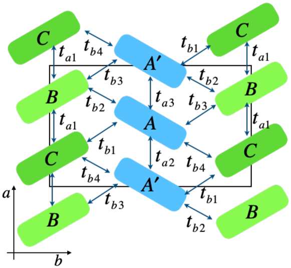
Figure 1: Conducting plane of BEDT-TTF molecules in $\alpha$-(BEDT-TTF)₂I₃ and the transfer energies between the molecules. The solid rectangle represents the unit cell. The crystal axes $a$ and $b$ are also shown.

Including the interaction terms to $H_{0}$, the conduction layer in $\alpha$-(BEDT-TTF)₂I₃ is described by the following extended Hubbard model[2]:

$$H = \sum\limits_{{\bm{k}},\alpha,\beta,\sigma}{{\varepsilon_{\alpha\beta}}\left({\bm{k}}\right)c_{{\bm{k}}\alpha\sigma}^{\dagger}{c_{{\bm{k}}\beta\sigma}}}+U\sum\limits_{j,\alpha}{c_{j\alpha\uparrow}^{\dagger}c_{j\alpha\downarrow}^{\dagger}{c_{j\alpha\downarrow}}{c_{j\alpha\uparrow}}}$$ (2)

$$+\sum\limits_{i,j,\alpha,\beta,\sigma,\sigma^{\prime}}{{V_{i\alpha,j\beta}}c_{i\alpha\sigma}^{\dagger}c_{j\beta\sigma^{\prime}}^{\dagger}{c_{j\beta\sigma^{\prime}}}{c_{i\alpha\sigma}}}.$$

The operator ${c_{{\bm{k}}\alpha\sigma}^{\dagger}}$ ( ${{c_{{\bm{k}}\alpha\sigma}}}$ ) creates (annihilates) an electron with the Bloch state ${\bm{k}}$ and spin $\sigma$ at molecule $\alpha$. The operator $c_{j\alpha\sigma}^{\dagger}$ ($c_{j\alpha\sigma}$) creates (annihilates) an electron with spin $\sigma$ at molecule $\alpha$ in the j-th unit cell. We assume that the system is subjected to uniaxial pressure along the $a$-axis [6]. ${\varepsilon_{\alpha\beta}}\left({\bf{k}}\right)$ are given by [2]

$${\varepsilon_{12}}\left({\bm{k}}\right) = {t_{a3}}{e^{-i{\bm{k}}\cdot{{\bm{d}}_{1}}}}+{t_{a2}}{e^{i{\bm{k}}\cdot{{\bm{d}}_{1}}}},$$ (3)

$${\varepsilon_{13}}\left({\bm{k}}\right) = {t_{b3}}{e^{-i{\bm{k}}\cdot{{\bm{d}}_{3}}}}+{t_{b2}}{e^{i{\bm{k}}\cdot{{\bm{d}}_{2}}}},$$ (4)

$${\varepsilon_{14}}\left({\bm{k}}\right) = {t_{b4}}{e^{-i{\bm{k}}\cdot{{\bm{d}}_{2}}}}+{t_{b1}}{e^{i{\bm{k}}\cdot{{\bm{d}}_{3}}}},$$ (5)

$${\varepsilon_{23}}\left({\bm{k}}\right) = {t_{b2}}{e^{-i{\bm{k}}\cdot{{\bm{d}}_{2}}}}+{t_{b3}}{e^{i{\bm{k}}\cdot{{\bm{d}}_{3}}}},$$ (6)

$${\varepsilon_{24}}\left({\bm{k}}\right) = {t_{b1}}{e^{-i{\bm{k}}\cdot{{\bm{d}}_{3}}}}+{t_{b4}}{e^{i{\bm{k}}\cdot{{\bm{d}}_{2}}}},$$ (7)

$${\varepsilon_{34}}\left({\bm{k}}\right) = {t_{a1}}{e^{i{\bm{k}}\cdot{{\bm{d}}_{1}}}}+{t_{a1}}{e^{-i{\bm{k}}\cdot{{\bm{d}}_{1}}}}.$$ (8)

Here, the transfer energies, $t_{\lambda}$ ($\lambda=a1,a2,...$), are pressure-dependent and can be expressed as follows:

$${t_{\lambda}}={C_{\lambda}}\left({1+{b_{\lambda}}P}\right).$$

The numerical coefficients $C_{\lambda}$ and $b_{\lambda}$ are as follows: For the molecule stacking direction: $C_{a1}=-0.028$, $b_{a1}=0.89$, $C_{a2}=0.048$, $b_{a2}=1.67$, $C_{a3}=-0.020$, $b_{a3}=-0.25$. For the other directions: $C_{b1}=0.123$, $b_{b1}=0$, $C_{b2}=0.140$, $b_{b2}=0.11$, $C_{b3}=-0.062$, $b_{b3}=0.32$, $C_{b4}=-0.025$, $b_{b4}=0$ [2]. $C_{\lambda}$ is given in units of eV, and the pressure $P$ is in units of GPa. These values are derived using an extrapolation formula [18], which is based on band calculations at ambient pressure [5] and crystal structure analysis under pressure[6]. As shown in Fig. 2(a), the vectors ${\bm{d}}_{1}$, ${\bm{d}}_{2}$, and ${\bm{d}}_{3}$ are defined as follows:

$${{\bm{d}}_{1}}=\left({0,\frac{a}{2}}\right),{{\bm{d}}_{2}}=\left({\frac{b}{2},-\frac{a}{4}}\right),{{\bm{d}}_{3}}=\left({\frac{b}{2},\frac{a}{4}}\right),$$ (9)

where $a$ and $b$ are the lattice constants along the $a$-axis and $b$-axis, respectively. We note that $a=9.19\AA$, $b=10.80\AA$, and $c=17.39\AA$ at ambient pressure.

The second term on the right-hand side of Eq. (2) represents the on-site Coulomb interaction, while the third term describes the nearest-neighbor interactions between different molecules. The parameters, $V_{i\alpha,j\beta}$, can take values of either $V_{c}$ or $V_{p}$, as shown in Fig. 2(b), depicting the interactions between molecule A and other molecules. The same set of interactions is also present among the other molecules.

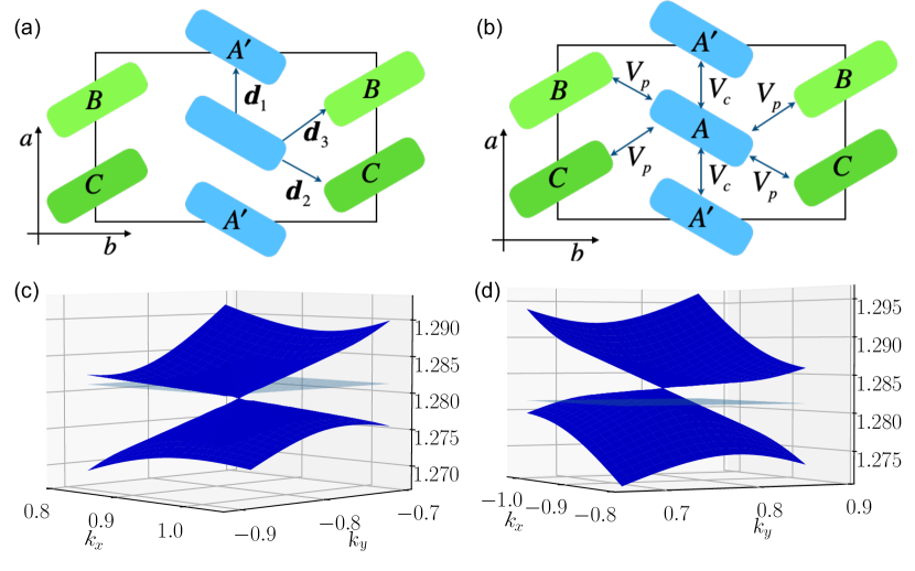
Figure 2: (a) Definition of three vectors, ${\bm{d}}_{1}$, ${\bm{d}}_{2}$, and ${\bm{d}}_{3}$ within the unit cell. (b) The nearest-neighbor interactions between molecule A and the other molecules. $V_{c}$ represents the interaction between A and A^′, while $V_{p}$ corresponds to the interactions between A and B, and A and C. The same set of interactions is also present for molecules A^′, B, and C. (c) and (d): The energy dispersions around the Dirac points obtained by the mean field calculation with $x=1$ and $P=0.8$ GPa. The energy dispersions are plotted around the Dirac points at (c) ${\bm{k}}_{D}^{(1)}=(0.939,-0.806)$ and (d) ${\bm{k}}_{D}^{(2)}=(-0.908,0.760)$. The thin horizontal plane represents the Fermi energy. In (c), the Dirac point is located below the Fermi energy, while in (d), the Dirac point is located above the Fermi energy.

Now, we apply a mean-field approximation to Eq. (2). The charge order at molecule $\alpha$ with spin $\sigma=\uparrow,\downarrow$ is defined as follows:

$${{n_{\alpha\sigma}}}=\frac{1}{N}\sum\limits_{\bm{k}}{\left\langle{c_{{\bm{k}}\alpha\sigma}^{\dagger}{c_{{\bm{k}}\alpha\sigma}}}\right\rangle},$$ (10)

Here, $N$ is the number of unit cells. This charge order plays a pivotal role in describing the insulating state at ambient pressure [19, 20]. However, under high pressures, the charge order exhibits a charge disproportionation [2].

The broken time-reversal symmetry and inversion symmetry are described by the following bond order parameter[12]:

$${\chi_{\alpha\sigma,\beta\sigma^{\prime},\pm}}=\frac{1}{N}\sum\limits_{\bm{k}}{{e^{-i{\bm{k}}\cdot{\bm{d}}_{\alpha\beta}^{\left(\pm\right)}}}\left\langle{c_{{\bm{k}}\alpha\sigma}^{\dagger}{c_{{\bm{k}}\beta\sigma^{\prime}}}}\right\rangle}.$$ (11)

We need to distinguish two bonds connecting molecule $\alpha$ and $\beta$. The vectors connecting molecule $\alpha$ and $\beta$ are denoted by ${\bm{d}}_{\alpha\beta}^{\left(\pm\right)}$. For example, ${\bm{d}}_{13}^{\left(+\right)}={{\bm{d}}_{2}}$ and ${\bm{d}}_{13}^{\left(-\right)}=-{{\bm{d}}_{3}}$. Regarding the interaction parameters, we adopt the assumption[2] that $U=0.4x$, $V_{c}=0.17x$, and $V_{p}=0.05x$, with these values expressed in units of eV. Here, the parameter $x$ controls the strength of the interaction. The case where $x=1$ results in charge disproportionation, which is consistent with the findings of NMR experiments[21]. We conduct self-consistent calculations for ${\chi_{\alpha\sigma,\beta\sigma^{\prime},\pm}}$ and $n_{\alpha\sigma}$.

III Broken time-reversal symmetry and inversion symmetry

The mean-field state breaks both time-reversal symmetry and inversion symmetry. Broken inversion symmetry is evident from the energy dispersion, as shown in Fig. 2(c) and (d), where we take $P=0.8$ GPa and $x=1$. In the $k_{x}$-$k_{y}$ plane, there exist two Dirac points. One Dirac point is located at ${\bm{k}}_{D}^{(1)}=(0.939,-0.806)$, and the other is at ${\bm{k}}_{D}^{(2)}=(-0.908,0.760)$. From these values, it is clear that inversion symmetry is broken since, if inversion symmetry were present, ${\bm{k}}_{D}^{(1)}=-{\bm{k}}_{D}^{(2)}$.

The energies at the Dirac points are as follows: ${E_{{\bm{k}}_{D}^{(1)}}}={\rm{1.279}}$ and ${E_{{\bm{k}}_{D}^{(2)}}}={\rm{1.283}}$, while the Fermi energy is ${E_{F}}={\rm{1.281}}$. There are electrons around the Dirac point at ${\bm{k}}_{D}^{(1)}$, and there are holes around the other Dirac point at ${\bm{k}}_{D}^{(2)}$. Note that the particle-hole symmetry is broken because $E_{F}-{E_{{\bm{k}}_{D}^{(1)}}}\neq{E_{{\bm{k}}_{D}^{(2)}}}-E_{F}$.

The broken time-reversal symmetry state is the flux state, as described below. We find that the spin degeneracy is not lifted, and the $\sigma=\uparrow$ states and $\sigma=\downarrow$ states remain decoupled: ${\chi_{\alpha\uparrow,\beta\uparrow^{\prime},\pm}}={\chi_{\alpha\downarrow,\beta\downarrow^{\prime},\pm}}$, ${\chi_{\alpha\uparrow,\beta\downarrow^{\prime},\pm}}=0$, and ${\chi_{\alpha\downarrow,\beta\uparrow^{\prime},\pm}}=0$. As a result, the following Hamiltonian is added to the kinetic energy term:

$${H_{\chi}} = -\frac{1}{2}\sum\limits_{{\bf{k}},\alpha\neq\beta,\sigma}\sum\limits_{s=\pm}{{V_{\alpha\beta}}}\left({\chi_{\alpha\uparrow,\beta\uparrow,s}^{*}+\chi_{\alpha\downarrow,\beta\downarrow,s}^{*}}\right)$$ (12)

$$\times{e^{i{\bf{k}}\cdot{\bf{d}}_{\alpha\beta}^{\left(s\right)}}}c_{{\bf{k}}\alpha\sigma}^{\dagger}{c_{{\bf{k}}\beta\sigma}}.$$

Here, $V_{\alpha\beta}$ represents the interaction parameter between molecule $\alpha$ and molecule $\beta$. In terms of ${\bf{d}}_{\alpha\beta}^{\left(s\right)}$, the term ${\varepsilon_{\alpha\beta}}\left({\bf{k}}\right)$ is rewritten as:

$${\varepsilon_{\alpha\beta}}\left({\bf{k}}\right)=\sum\limits_{s=\pm}{{t_{\alpha\beta s}}{e^{i{\bf{k}}\cdot{\bf{d}}_{\alpha\beta}^{\left(s\right)}}}},$$ (13)

with ${t_{13+}}={t_{b2}}$, ${t_{13-}}={t_{b3}}$, and so forth. Upon including $H_{\chi}$, the term ${{t_{\alpha\beta s}}}$ is replaced by $t_{\alpha\beta s}^{{\rm{eff}}}$, where

$$t_{\alpha\beta s}^{{\rm{eff}}}={t_{\alpha\beta s}}-\frac{1}{2}{V_{\alpha\beta}}\left({\chi_{\alpha\uparrow,\beta\uparrow,s}^{*}+\chi_{\alpha\downarrow,\beta\downarrow,s}^{*}}\right).$$ (14)

An effective hopping parameter, $t_{\alpha\beta\pm}^{{\rm{eff}}}$, is introduced, which combines the original hopping parameter $t_{\lambda}$ with the bond order parameter ${\chi_{\alpha\sigma,\beta\sigma^{\prime},\pm}}$. Using $t_{\alpha\beta\pm}^{{\rm{eff}}}$, we define the product of three effective hopping parameters around each triangular plaquette. For instance,

$${\chi_{124}^{(-)}}=t_{14+}^{{\rm{eff}}}t_{42-}^{{\rm{eff}}}t_{21-}^{{\rm{eff}}}.$$ (15)

We define this product in the counterclockwise direction. Additionally, there is another plaquette involving molecules 1, 2, and 4. That is,

$${\chi_{124}^{(+)}}=t_{12+}^{{\rm{eff}}}t_{24-}^{{\rm{eff}}}t_{41+}^{{\rm{eff}}}.$$ (16)

In Fig. 4(a), left panel, a horizontal dashed line divides the unit cell into an upper part and a lower part. The $\pm$ sign in $\chi_{\alpha\beta\gamma}^{(\pm)}$ refers to the two plaquettes within the unit cell. Specifically, the $+$ sign corresponds to the plaquettes located in the upper region, while the $-$ sign corresponds to those in the lower region. The argument of the complex number ${\chi_{\alpha\beta\gamma}^{(\pm)}}$ is denoted by ${\Phi_{\alpha\beta\gamma}^{(\pm)}}$ and is defined by

$${\chi_{\alpha\beta\gamma}^{(\pm)}}=\left|{{\chi_{\alpha\beta\gamma}^{(\pm)}}}\right|\exp\left({i{\Phi_{\alpha\beta\gamma}^{(\pm)}}}\right).$$ (17)

${\Phi_{\alpha\beta\gamma}^{(\pm)}}$ takes either 0 or $\pi$ for the non-interacting case [22].

The time-reversal symmetry is broken within the unit cell, as shown in Fig. 4(a) (left panel). The flux pattern of ${\Phi_{\alpha\beta\gamma}^{(\pm)}}$ is depicted in Fig. 4(a), where plaquettes with pink color indicate ${\Phi_{\alpha\beta\gamma}^{(\pm)}}>0$, and blue color indicates ${\Phi_{\alpha\beta\gamma}^{(\pm)}}<0$. Subtle variations in hue represent deviations from $\pm\pi$. Within each unit cell, the fluxes collectively sum to zero: ${\chi_{124}^{(+)}}$ offsets ${\chi_{124}^{(-)}}$. Similarly, ${\chi_{123}^{(+)}}$ offsets ${\chi_{123}^{(-)}}$. Concomitantly, ${\chi_{134}^{(\pm)}}$ offsets ${\chi_{234}^{(\mp)}}$.

While time-reversal symmetry is broken within the unit cell, the translational symmetry remains unbroken, as shown in the right panel of Fig. 4(a). We note that a similar time-reversal symmetry breaking is discussed on the high-$T_{c}$ cuprates[23]. The dependence of the flux values on the interaction strength is demonstrated in Fig. 4(b). We confirmed from the calculation with $U=0$ (not shown) that the nearest-neighbor interactions $V_{c}$ and $V_{p}$ play a central role in breaking time-reversal symmetry. Regarding the temperature dependence of the flux values, Fig. 4(c) presents the results. Notably, there is no phase transition within the temperature range displayed in this figure. Time-reversal symmetry is already broken at high temperatures.

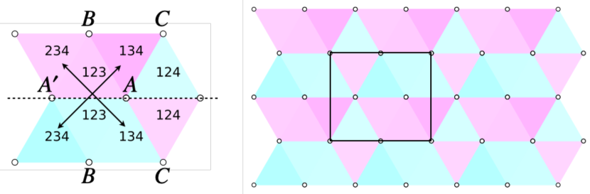
Figure 3: Left panel: The flux configuration in the unit cell, with open circles representing molecules. Each plaquette is labeled with three numbers denoting $\alpha$, $\beta$, and $\gamma$ of ${\chi_{\alpha\beta\gamma}}$. Plaquettes colored in pink denote positive flux values, while those in blue signify negative flux values. Subtle variations in hue represent deviations from $\pm\pi$. The pairs of plaquettes connected by arrows indicate that the fluxes of these two plaquettes have opposite signs and thus cancel each other out. Right panel: Flux patterns in unit cells are shown, exhibiting translational symmetry. The solid rectangle represents the unit cell.

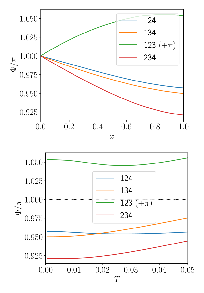
Figure 4: Upper panel: Dependence of the flux values on the interaction. Only flux values where ${\Phi_{\alpha\beta\gamma}}>0$ are shown. The value of ${\Phi_{123}}$ is shifted by $\pi$. Lower panel: Temperature dependence of the flux values.

From a detailed analysis of $t_{\alpha\beta\pm}^{{\rm{eff}}}$, we find that the breaking of time-reversal symmetry originates from the symmetry breaking in the hopping between A and A^′. That is,

$$t_{12+}^{{\rm{eff}}}\neq\left(t_{21-}^{{\rm{eff}}}\right)^{*}.$$ (18)

We note that the symmetry breaking in $n_{A}=n_{A\uparrow}+n_{A\downarrow}$ and $n_{A^{\prime}}=n_{{A^{\prime}}\uparrow}+n_{{A^{\prime}}\downarrow}$ leads to stripe charge order under ambient pressure [19, 20, 24]. However, at high pressure, this symmetry breaking is replaced by the breaking of time-reversal and inversion symmetries.

Now we discuss the reliability of our mean field calculations. To incorporate the effects of strong electronic correlation, we have integrated the slave-rotor theory[25] into our mean field approach. This enhanced analysis has been compared with experimental results[26]. A key finding is that strong coupling effects lead to a reduction in the Fermi velocity, which characterizes the velocity of the Dirac fermions. This effect aligns with the renormalization group theory[27]. Notably, at a finite pressure of around 0.6 GPa, the system transitions into an insulating state. We have compared the pressure dependence of the Fermi velocity with experimental data, where the Fermi velocity is estimated from the analysis of Shubnikov-de Haas oscillations in doped samples. Our theoretical results show good agreement with these experimental findings. However, it is important to note that the impact of strong coupling effects becomes less significant at higher pressures and is negligible at pressures equal to or greater than 0.8 GPa. We have also conducted mean field calculations that include the possibility of antiferromagnetic long-range order. These calculations revealed that such a state is unstable at pressures above 0.6 GPa.

As for the stability of the flux state, we comment on the pivotal role of off-site Coulomb $V$ interactions in the emergence of the flux state in $\alpha$-(BEDT-TTF)₂I₃. The stability of the flux state, as compared to the charge-ordered state, can be attributed to the specific characteristics of the density of states (DOS) at the Fermi energy. Notably, the DOS vanishes at the Dirac point, where the Fermi energy lies in the absence of the interactions. This phenomenon significantly impedes the stabilization of a charge-ordered state. In contrast, the flux state, which originates from phase modifications in the hopping parameters, exhibits a relatively independent stability of the DOS. This distinction is crucial for understanding the preferential formation of the flux state under these conditions.

Now we discuss the distinctions between our flux state and the topological Mott insulators[28]. In the model of topological Mott insulators, a flux value of $\pm\pi/2$ is specifically chosen to create a gap within the Dirac fermion spectrum. By contrast, our study investigates a flux state characterized by a non-zero flux value, which does not inherently result in a gap. This difference is primarily due to the vanishing DOS in the non-interacting system, a factor that significantly influences the behavior and properties of the flux state under consideration.

IV Thermopower and Nernst signal

The experimental verification of broken time-reversal symmetry is a crucial question to address. However, since this state is realized under high pressure, it requires the use of a pressure cell, making direct verification extremely difficult. Nevertheless, the presence of broken time-reversal symmetry can be inferred through thermal transport measurements. In the absence of broken time-reversal symmetry, we would anticipate a vanishing thermopower $S_{xx}$ while observing a large Nernst signal $S_{xy}$ when the chemical potential is at the Dirac point [29, 30]. Conversely, if there is a chemical potential shift, and the shift exceeds the Zeeman energy, we expect to observe a large thermopower and a vanishing Nernst signal. In the time-reversal symmetry broken state considered in this study, there is asymmetry in the shifts of the two Dirac point energies concerning the Fermi energy, along with a difference in their absolute values. In this case, a pronounced Nernst signal and thermopower are anticipated, with the Nernst signal exceeding the thermopower.

We compute $S_{xx}$ and $S_{xy}$ as follows: In the presence of the electric field ${\bm{E}}$ and the temperature gradient $\nabla T$, the electric current is given by

$${\bm{j}}=\sigma{\bm{E}}+\alpha(-\nabla T),$$ (19)

in the linear response regime. Here, $\sigma$ and $\alpha$ are the electrical and thermoelectric conductivity tensors, respectively. We first compute the zero-temperature conductivity, $\sigma_{ij}(\varepsilon_{F})$, where $\varepsilon_{F}$ is the Fermi energy, using the Kubo formula. Subsequently, we obtain $\sigma$ and $\alpha$ at temperature $T$ and with chemical potential $\mu$ using the following equations [31, 29]:

$${\sigma_{ij}}\left({T,\mu}\right)=\int{d\varepsilon}{\sigma_{ij}}\left(\varepsilon\right)\left({-\frac{{\partial f\left(\varepsilon\right)}}{{\partial\varepsilon}}}\right),$$

$${\alpha_{ij}}\left({T,\mu}\right)=-\frac{1}{{eT}}\int{d\varepsilon}{\sigma_{ij}}\left(\varepsilon\right)\left({\varepsilon-\mu}\right)\left({-\frac{{\partial f\left(\varepsilon\right)}}{{\partial\varepsilon}}}\right).$$

Here, $f\left(\varepsilon\right)=1/\left[{\exp\left({\beta\left({\varepsilon-\mu}\right)}\right)+1}\right]$ is the Fermi distribution function and $\beta=1/(k_{\rm B}T)$ with $k_{\rm B}$ being the Boltzmann constant. For the calculation of the zero-temperature conductivity, $\sigma_{ij}(\varepsilon_{F})$, we consider Landau levels with broadening due to impurity scattering. We assume the Landau levels of massless Dirac fermions of the continuum model, with parameters such as the Fermi velocity $v_{F}$ and the energy of the Dirac point $E_{D}$. For the two Dirac points present, we represent $E_{D}$ for each Dirac point as $E_{D}^{(1)}$ and $E_{D}^{(2)}$. Although the Dirac cones in $\alpha$-(BEDT-TTF)₂I₃ are tilted [32], the effect of the tilt is merely to renormalize the Fermi velocity [33, 34]. To account for the broadening, we assume the Lorentz function with energy-independent damping, $\Gamma$, for simplicity. In this simplified calculation, the peak in the longitudinal conductivity $\sigma_{xx}$ at $\varepsilon_{F}=0$ is underestimated, but there is no qualitative change when compared to the more elaborate calculation [29]. $S_{xx}$ and $S_{xy}$ are calculated using

$$S_{ij}=\left(\sigma^{-1}\alpha\right)_{ij}.$$ (20)

Figure 5 presents the temperature dependence of $S_{xx}$ and $S_{xy}$ for different magnetic fields. The crucial point to note is that both $S_{xx}$ and $S_{xy}$ exhibit large values, with $S_{xy}$ being several times larger than $S_{xx}$. Here, we set the Fermi velocity $v_{F}=5\times 10^{4}\,{\rm m}\,{\rm s}^{-1}$ for both Dirac cones. The values for $E_{D}^{(1)}$ and $E_{D}^{(2)}$ are $E_{D}^{(1)}=0.8$ meV and $E_{D}^{(2)}=-0.7$ meV, respectively. The Landau level broadening parameter is taken as $\Gamma=0.1$ meV.

In the experiment[17], the temperature dependence of the Nernst signal $S_{xy}$ displays a peak around $T\simeq 10$ K under magnetic field. This peak emerges when the magnetic field exceeds 0.5 T, with its maximum observed around 10 T. This maximum value is notably large, surpassing 3 mV/K at 13 T and 11 K. Concurrently, the temperature dependence of the thermopower $S_{xx}$ also exhibits a peak around $T\simeq 10$ K under magnetic field. The peak value of $S_{xx}$, measured at 13 T and 11 K, is less than one-sixth that of $S_{xy}$. These characteristics are consistent with our theoretical results. In our computations, the primary parameters are $E_{D}^{(1)}$ and $E_{D}^{(2)}$. The values specified above closely replicate the peak positions and magnitudes of $S_{xy}$ and $S_{xx}$. When we take either $E_{D}^{(1)}=-E_{D}^{(2)}\neq 0$ or $E_{D}^{(1)}=E_{D}^{(2)}=0$, $S_{xx}$ vanishes. Meanwhile, if we take $E_{D}^{(1)}=E_{D}^{(2)}\neq 0$, $S_{xy}$ is much smaller than $S_{xx}$. To be consistent with the experimental observations, we require opposite signs and disparate absolute values for $E_{D}^{(1)}$ and $E_{D}^{(2)}$. This distinction is a direct result of our symmetry-broken phase. A limitation of our calculation lies in the assumption of a constant $\Gamma$. Indeed, to account for the diminishing peak values in $S_{xy}$ and $S_{xx}$ at high magnetic fields[17], we must consider its variability. This aspect will be addressed in subsequent research.

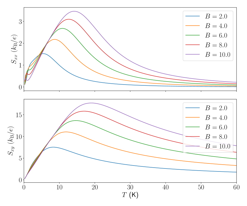
Figure 5: The thermopower $S_{xx}$ (upper panel) and the Nernst signal $S_{xy}$ (lower panel) as functions of temperature for different magnetic fields, with the magnetic field measured in tesla. Both $S_{xx}$ and $S_{xy}$ are expressed in units of $k_{\rm B}/e=86.17~{}\mu$V K^-1. We take $E_{D}^{(1)}=0.8~{}$meV, $E_{D}^{(2)}=-0.7~{}$meV, and $\Gamma=0.1$ meV.

V Conclusion

In conclusion, our study reveals that the ground state of $\alpha$-(BEDT-TTF)₂I₃ under pressure breaks both time-reversal symmetry and particle-hole symmetry while maintaining translational symmetry. This symmetry breaking arises from the creation of fluxes that deviate from 0 or $\pm\pi$ within a unit cell. To experimentally confirm this symmetry breaking state, we have calculated the thermopower and the Nernst signal, and our results are in good agreement with the experimental observations [17]. This agreement provides substantial support for our theoretical prediction regarding the symmetry broken state.