Enhancing Graph Transformers with Hierarchical Distance Structural Encoding

Abstract

Graph transformers need strong inductive biases to derive meaningful attention scores. Yet, current methods often fall short in capturing longer ranges, hierarchical structures, or community structures, which are common in various graphs such as molecules, social networks, and citation networks. This paper presents a Hierarchical Distance Structural Encoding (HDSE) method to model node distances in a graph, focusing on its multi-level, hierarchical nature. We introduce a novel framework to seamlessly integrate HDSE into the attention mechanism of existing graph transformers, allowing for simultaneous application with other positional encodings. To apply graph transformer with HDSE to large-scale graphs, we further propose a hierarchical global attention mechanism with linear complexity. We theoretically prove the superiority of HDSE over shortest path distances in terms of expressivity and generalization. Empirically, we demonstrate that graph transformers with HDSE excel in graph classification, regression on 7 graph-level datasets, and node classification on 12 large-scale graphs, including those with up to a billion nodes. We provide our code in the supplementary and will make it publicly available upon acceptance.

1 Introduction

The success of Transformers (Vaswani et al., 2017) in various domains, including natural language processing (NLP) and computer vision (Dosovitskiy et al., 2020), has sparked significant interest in developing transformers for graph data (Dwivedi & Bresson, 2020; Ying et al., 2021; Kreuzer et al., 2021; Chen et al., 2022a; Rampášek et al., 2022; Ma et al., 2023a; Zhang et al., 2023; Wu et al., 2023b). Scholars have turned their attention to this area, aiming to address the limitations of Message-Passing Graph Neural Networks (MPNNs) (Gilmer et al., 2017) such as over-smoothing (Li et al., 2018) and over-squashing (Alon & Yahav, 2020; Topping et al., 2021).

However, Transformers (Vaswani et al., 2017) are known for their lack of strong inductive biases (Dosovitskiy et al., 2020). In contrast to MPNNs, graph transformers do not rely on fixed graph structure information. Instead, they compute pairwise interactions for all nodes within a graph and represent positional and structural data using more flexible, soft inductive biases. Despite its potential, this mechanism does not have the capability to learn hierarchical structures within graphs. Developing effective positional encodings is also challenging, as it requires identifying important hierarchical structures among nodes, which differ significantly from other Euclidean domains (Bronstein et al., 2021). Consequently, graph transformers are prone to overfitting and often underperform MPNNs when data is limited (Ma et al., 2023a), especially in tasks involving large graphs with relatively few labeled nodes (Wu et al., 2023b). These challenges become even more significant when dealing with various molecular graphs, such as those found in polymers or proteins. These graphs are characterized by a multitude of substructures and exhibit long-range and hierarchical structures. The inability of graph transformers to learn these hierarchical structures can significantly impede their performance in tasks involving such complex molecular graphs.

Further, the global all-pair attention mechanism in transformers poses a significant challenge due to its time and space complexity, which increases quadratically with the number of nodes. This quadratic complexity significantly restricts the application of graph transformers to large graphs, as training them on graphs with millions of nodes can require substantial computational resources. Large-scale graphs, such as social networks and citation networks, often exhibit community structures characterized by closely interconnected groups with distinct hierarchical properties. To enhance the scalability and effectiveness of graph transformers, it is crucial to incorporate hierarchical structural information at various levels.

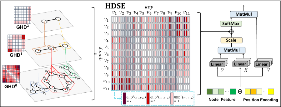
Figure 1: Overview of our proposed Hierarchical Distance Structural Encoding (HDSE) and its integration with graph transformers. HDSE uses the graph hierarchy distance (GHD, refer to Definition 3.1) that can capture interpretable patterns in graph-structured data by using diverse graph coarsening algorithms. Darker colors indicate longer distances.

To address the aforementioned challenges and unlock the true potential of the transformer architecture in graph learning, we propose a hierarchy distance structural encoding (HDSE) method (Sec. 3.1), which can be combined with various graph transformers to produce more expressive node embeddings. HDSE encodes the hierarchy distance, a metric that measures the distance between nodes in a graph, taking into account multi-level graph hierarchical structures. We utilize popular coarsening methods (Karypis & Kumar, 1998; Ng et al., 2001; Girvan & Newman, 2002; Blondel et al., 2008; Loukas, 2019) to construct graph hierarchies, enabling us to measure the distance relationship between nodes across various hierarchical levels.

HDSE enables us to incorporate a robust inductive bias into existing transformers and address the issue of lacking canonical positioning. To achieve this, we introduce a novel framework (Sec. 3.2), as illustrated in Figure 1. We utilize an end-to-end trainable function to encode HDSE as structural bias weights into the attentions, allowing the graph transformer to integrate both HDSE and other positional encodings simultaneously. Our theoretical analysis demonstrates that graph transformers equipped with HDSE are significantly more powerful than the ones with the commonly used shortest path distances, in terms of both expressiveness and generalization. Furthermore, extensive experiments on 7 graph-level tasks show that HDSE effectively enhances various types of baseline transformers.

To enable the application of graph transformers with HDSE to large graphs ranging from millions to billions of nodes, we introduce a simple yet efficient HGT-HDSE model (Sec. 3.3), equipped with a hierarchical global attention mechanism with linear complexity. The use of hierarchical structures preserves structural information and widens the receptive field, avoiding over-squashing. Meanwhile, it allows for the use of multi-hop features, preventing over-smoothing. Our HGT-HDSE model exhibits high efficiency and quality across 12 large-scale node classification datasets, with sizes up to the billion-node level.

2 Background and Related Works

We refer to a graph as a tuple $G=(V,E,\mathbf{X})$, with node set $V$, edge set $E\subseteq V\times V$, and node features $\mathbf{X}\in\mathbb{R}^{|V|\times d}$. Each row in $\mathbf{X}$ represents the feature vector of a node, with $|V|$ denoting the number of nodes and feature dimension $d$. The features of node $v$ are denoted by $x_{v}\in\mathbb{R}^{d}$.

2.1 Graph Hierarchies

Given an input graph $G$, a graph hierarchy of $G$ consists of a sequence of graphs $(G^{k},\phi_{k})_{k\geq 0}$, where $G^{0}=G$ and $\phi_{k}:V^{k}\to V^{k+1}$ are surjective node mapping functions. Each node $v^{k+1}_{j}\in V^{k+1}$ represents a cluster of a subset of nodes $\{v^{k}_{i}\}\subseteq V^{k}$. This partition can be described by a projection matrix $\hat{P}^{k}\in\{0,1\}^{{|V^{k}|\times|V^{k+1}|}}$, where $\hat{P}^{k}_{ij}=1$ if and only if $v^{k+1}_{j}=\phi_{k}(v^{k}_{i})$. The normalized version can be defined by $P^{k}=\hat{P}^{k}{C^{k}}^{-{1/2}}$, where $C^{k}\in\mathbb{R}^{{|V^{k+1}|\times|V^{k+1}|}}$ is a diagonal matrix with its $j$-th diagonal entry being the cluster size of $v^{k+1}_{j}$. We define the node feature matrix $\mathbf{X}^{k+1}$ for $G^{k+1}$ by $\mathbf{X}^{k+1}={P^{k}}^{\top}\mathbf{X}^{k}$, where each row of $\mathbf{X}^{k+1}$ represents the average of all entries within a specific cluster. The edge set $E^{k+1}$ of $G^{k+1}$ is defined as $E^{k+1}=\{(u^{k+1},v^{k+1})|\exists v^{k}_{r}\in\phi_{k}^{-1}(u^{k+1}),v^{k}_{s}\in\phi_{k}^{-1}(v^{k+1}),\text{ such that }(v^{k}_{r},v^{k}_{s})\in E^{k}\}$.

Graph hierarchies can be constructed by repeatedly applying graph coarsening algorithms. These algorithms take a graph, $G^{k}$, and generate a mapping function $\phi_{k}:V^{k}\rightarrow V^{k+1}$, which maps the nodes in $G^{k}$ to the nodes in the coarser graph $G^{k+1}$. A summary and comparison of popular graph coarsening algorithms, along with their computational complexities, can be found in Table 1. We define the coarsening ratio as $\alpha=\frac{|V^{k+1}|}{|V^{k}|}$, which represents the proportion of the number of nodes in the coarser graph $G^{k+1}$ to the number of nodes in the original graph $G^{k}$. Consequently, each graph $G^{k}$, where $k>0$, captures specific substructures derived from the preceding graph. Empirically, it is worth noting that we mainly focus on a maximal hierarchy level of $K=1$. This choice aligns with related works (Zhang et al., 2022; Zhu et al., 2023) and has showed good performance in our evaluation.

Table 1: Comparison of popular graph coarsening algorithms.

Coarsening algorithm	Complexity
METIS (Karypis & Kumar, 1998)	$O(|E|)$
Spectral Clustering (Ng et al., 2001)	$O(|V|^{3})$
Loukas (Loukas, 2019)	$O(|V|)$
Newman (Girvan & Newman, 2002)	$O(|E|^{2}|V|)$
Louvain Method (Blondel et al., 2008)	$O(|V|\log|V|)$

2.2 Graph Transformers

Transformers (Vaswani et al., 2017) have recently gained significant attention in graph learning, due to their ability to learn intricate relationships that extend beyond the capabilities of conventional GNNs, and in a unique way. The architecture of these models primarily contain a self-attention module and a feed-forward neural network, each of which is followed by a residual connection paired with a normalization layer. Formally, the self-attention mechanism involves projecting the input node features $\mathbf{X}$ using three distinct matrices $\mathrm{W}_{\mathbf{Q}}\in\mathbb{R}^{d\times d^{\prime}}$, $\mathrm{W}_{\mathbf{K}}\in\mathbb{R}^{d\times d^{\prime}}$ and $\mathrm{W}_{\mathbf{V}}\in\mathbb{R}^{d\times d^{\prime}}$, resulting in the representations for query ($\mathbf{Q}$), key ($\mathbf{K}$), and value ($\mathbf{V}$), which are then used to compute the output features described as follows:

$$\mathbf{Q}=\mathbf{X}\mathrm{W}_{\mathbf{Q}},\ \mathbf{K}=\mathbf{X}\mathrm{W}_{\mathbf{K}},\ \mathbf{V}=\mathbf{X}\mathrm{W}_{\mathbf{V}},$$

$$\mathrm{Attention}\left(\mathbf{X}\right)=\mathrm{softmax}\left(\frac{\mathbf{QK}^{\top}}{\sqrt{d^{\prime}}}\right)\mathbf{V}.$$ (1)

Technically, transformers can be considered as message-passing GNNs operating on fully-connected graphs, decoupled from the input graphs. The main research question in the context of graph transformers is how to incorporate the structural bias of the given input graphs by adapting the attention mechanism or by augmenting the original features. The Graph Transformer (GT) (Dwivedi & Bresson, 2020) represents an early work using Laplacian eigenvectors as positional encoding (PE), and various extensions and alternative models have been proposed since then (Min et al., 2022). For instance, the structure-aware transformer (SAT) (Chen et al., 2022a) extracts a subgraph representation rooted at each node before computing the attention. Most initial works in the area focus on the classification of smaller graphs, such as molecules; yet, recently, GraphGPS (Rampášek et al., 2022) and follow-up works (Zhao et al., 2021a; Wu et al., 2022, 2023a, 2023b; Chen et al., 2022b; Kong et al., 2023; Shirzad et al., 2023) also consider larger graphs.

2.3 Hierarchy in Graph Learning

In message passing GNNs, hierarchical pooling of node representations is a proven method for incorporating coarsening into reasoning (Bianchi et al., 2020; Gao & Ji, 2019; Ying et al., 2018; Lee et al., 2019; Huang et al., 2019; Ranjan et al., 2020). With GNNs, coarsened graph representations are further considered in the context of molecules (Jin et al., 2020) and virtual nodes (Hwang et al., 2022). Additionally, Bai et al. (2022) employ graph hierarchies to develop a novel graph kernel by transitively aligning the nodes across multi-level hierarchical graphs. The recent HC-GNN (Zhong et al., 2023) demonstrates competitive performance in node classification on large-scale graphs, utilizing hierarchical community structures for message passing.

In graph transformers, there are currently only a few hierarchical models. Zhang et al. (2022) use adaptive node sampling in their graph transformer, enabling it for large-scale graphs and capturing long-range dependencies. Their ANS-GT groups nodes into super-nodes and allows for interactions between them. Similarly, HSGT (Zhu et al., 2023) aggregates multi-level graph information and employs graph hierarchical structure to construct intra-level and inter-level transformer blocks. The intra-level block facilitates the exchange and transformation of information within the local context of each node, while the inter-level block adaptively coalesces every substructure present. Our concurrent work directly incorporates hierarchy into the attention, a fundamental building block of the transformer architecture, making it flexible and applicable to existing graph transformers. Additionally, Coarformer (Kuang et al., 2021) utilizes graph coarsening techniques to generate coarse views of the original graph, which are subsequently used as input for the transformer model. Likewise, PatchGT (Gao et al., 2022) starts by segmenting graphs into patches using spectral clustering and then learns from these non-trainable graph patches. MGT (Ngo et al., 2023) learns atomic representations and groups them into meaningful clusters, which are then fed to a transformer encoder to calculate the graph representation. However, these approaches typically yield coarse-level representations that lack comprehensive awareness of the original node-level features (Jiang et al., 2023). In contrast, our model integrates hierarchical information from a broader distance perspective, thereby avoiding the oversimplification in these coarse-level representations.

3 Our Method

3.1 Hierarchy Distance Structural Encoding (HDSE)

Firstly, we introduce a novel concept called graph hierarchy distance (GHD), which is defined as follows.

Definition 3.1 (Graph Hierarchy Distance).

Given two nodes $u,v$ in graph $G$, and a graph hierarchy $(G^{i},\phi_{i})_{i\geq 0}$, the $k$-level hierarchy distance between $u$ and $v$ is defined as

$$\mathrm{GHD}^{0}\left(u,v\right) =\mathrm{SPD}\left(u,v\right),$$

$$\mathrm{GHD}^{k}\left(u,v\right) =\mathrm{SPD}\left(\phi_{k-1}...\phi_{0}(u),\phi_{k-1}...\phi_{0}(v)\right),$$ (2)

where $\mathrm{SPD}\left(\cdot,\cdot\right)$ is the shortest path distance between two nodes ($\infty$ if the nodes are not connected), and $\phi_{k-1}...\phi_{0}(\cdot)$ maps a node in $G^{0}$ to a node in $G^{k}$.

Note that the $k$-level hierarchy distance adheres to the definition of a metric, being zero for $v=u$, invariably positive, symmetric, and fulfilling the triangle inequality. As illustrated on the left side of Figure 1, it can be observed that $\mathrm{GHD}^{0}\left(v_{1},v_{11}\right)=7$, whereas $\mathrm{GHD}^{1}\left(v_{1},v_{11}\right)=2$.

Graph hierarchies have been observed to assist in identifying community structures in graphs that exhibit a clear property of tightly knit groups, such as social networks and citation networks (Girvan & Newman, 2002). They may also aid in prediction over graphs with a clear hierarchical structure, such as metal–organic frameworks or proteins. Fig. 2 shows that with the graph hierarchies generated by the Newman coarsening method, $\mathrm{GHD}^{1}$ is capable of capturing chemical motifs, including CF3 and aromatic rings.

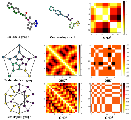
Figure 2: Examples of graph coarsening results and hierarchy distances. Top: HDSE can capture chemical motifs such as CF3 and aromatic rings on molecule graphs. Bottom: HDSE can distinguish the Dodecahedron and Desargues graphs. The Dodecahedral graph has 1-level hierarchy distances of length 2 (indicated by the dark color), while the Desargues graph doesn’t. In contrast, the GD-WL test with SPD cannot distinguish these graphs (Zhang et al., 2023).

Based on GHD, we propose hierarchy distance structural encoding (HDSE), defined for each pair of nodes $i,j\in V$:

$$\mathrm{D}_{i,j}=\left[\mathrm{GHD}^{0},\mathrm{GHD}^{1},...,\mathrm{GHD}^{K}\right]_{i,j}\in\mathbb{R}^{K+1},$$ (3)

where $\mathrm{GHD}^{k}$ is the $k$-level hierarchy distance matrix, and $K\in\mathbb{N}$ controls the maximum level of hierarchy considered.

We demonstrate the superior expressiveness of HDSE over SPD using recently proposed graph isomorphism tests inspired by the Weisfeiler-Leman algorithm (Weisfeiler & Leman, 1968). In particular, Zhang et al. (2023) introduced the Generalized Distance Weisfeiler-Leman (GD-WL) Test and applied it to analyze a graph transformer architecture that employs $\mathrm{SPD}(i,j)$ as relative positional encodings. They proved that the graph transformer’s maximum expressiveness is the GD-WL test with SPD. Here, we also use the GD-WL test to showcase the expressiveness of HDSE.

Proposition 3.2 (Expressiveness of HDSE).

GD-WL with HDSE $(\mathrm{D}_{i,j})$ is strictly more expressive than GD-WL with the shortest path distance $\mathrm{SPD}(i,j)$.

The proof is provided in Appendix A.1. Firstly, we show that the GD-WL test using HDSE can differentiate between any two graphs that can be distinguished by the GD-WL test with SPD. Next, we show that the GD-WL test with HDSE is capable of distinguishing the Dodecahedron and Desargues graphs (Figure 2) while the one with SPD cannot.

3.2 Integrating HDSE in Graph Transformers

We integrate HDSE ($\mathrm{D}_{i,j}$) into the attention mechanism of each graph transformer layer to bias each node update. To achieve this, we use an end-to-end trainable function $\mathrm{Bias}:\mathbb{R}^{K+1}\rightarrow\mathbb{R}$ to learn the biased structure weight $\mathrm{H}_{i,j}=\mathrm{Bias}(\mathrm{D}_{i,j})$. We limit the maximum distance length to a value $L$, based on the hypothesis that detailed information loses significance beyond a certain distance. By imposing this limit, the model can extend acquired patterns to graphs of varying sizes not encountered in training. Specificially, we implement the function $\mathrm{Bias}$ using an MLP as follows:

$$\mathrm{H}_{i,j} =\mathrm{MLP}\left(\left[\mathbf{e}^{0}_{\mathrm{clip}^{0}_{i,j}},\cdots,\mathbf{e}^{K}_{\mathrm{clip}^{K}_{i,j}}\right]\right)\in\mathbb{R},$$

$$\mathrm{clip}^{k}_{i,j} =\min\left(L,\mathrm{GHD}^{k}_{i,j}\right),0\leq k\leq K,$$ (4)

where ${\left[\mathbf{e}^{k}_{0},\mathbf{e}^{k}_{1},\cdots,\mathbf{e}^{k}_{L}\right]}_{0\leq k\leq K}\in\mathbb{R}^{d\times(L+1)}$ collects $L+1$ learnable feature embedding vectors $\mathbf{e}^{k}_{i}$ for hierarchy level $k$. By embedding the hierarchy distances at different levels into learnable feature vectors, it may enhance the aggregation of multi-level graph information among nodes and expands the receptive field of nodes to a larger scale. We assume single-headed attention for simplified notation, but when extended to multiheaded attention, one bias is learned per distance per head.

We incorporate the learned biased structure weights $H$ to graph transformers, using the popular biased self-attention method proposed by Ying et al. (2021), formulated as:

$$\mathrm{Attention}\left(\mathbf{X}\right)=\mathrm{softmax}\left(\mathrm{A}+\mathrm{H}\right)\mathbf{V},\mathrm{A}=\frac{\mathbf{QK}^{\top}}{\sqrt{d^{\prime}}},\\$$ (5)

where the original attention score $\mathrm{A}$ is directly augmented with $\mathrm{H}$. This approach is backbone-agnostic and can be seamlessly integrated into the self-attention mechanism of existing graph transformer architectures. Notably, we have the following results on expressiveness and generalization.

Proposition 3.3.

The power of a graph transformer with HDSE to distinguish non-isomorphic graphs is at most equivalent to that of the GD-WL test with HDSE. With proper parameters and an adequate number of heads and layers, a graph transformer with HDSE can match the power of the GD-WL test with HDSE.

See the proof in Appendix A.2. This result provides a precise characterization of the expressivity power and limitations of graph transformers with HDSE. Combining Proposition 3.2 and 3.3 immediately yields the following corollary:

Corollary 3.4 (Expressiveness of Graph Transformers with HDSE).

There exists a graph transformer using HDSE (with fixed parameters), denoted as $\mathcal{M}$, such that $\mathcal{M}$ is more expressive than graph transformers with the same architecture using SPD, regardless of their parameters.

This is a fine-grained expressiveness result of graph transformers with HDSE. It demonstrate the superior expressiveness of HDSE over SPD in graph transformers.

Proposition 3.5 (Generalization of Graph Transformers with HDSE).

(Informal) For a semi-supervised binary node classification problem, suppose the label of each node $i\in V$ is determined by node features in the “hierarchical core neighborhood” $S_{*}^{i}=\{j:\mathrm{D}_{i,j}=D*\}$ for a certain $d^{*}$, where $\mathrm{D}_{i,j}$ is HDSE defined in (3). Then, a properly initialized one-layer graph transformer equipped with HDSE can learn such graphs with a desired generalization error, while using SPD cannot guarantee satisfactory generalization.

The formal version and the proof are given in Appendix A.3. Proposition 3.5 is a corollary and extension of Theorem 4.1 of Li et al. (2023) from SPD to HDSE. It indicates that learning with HDSE can capture the labeling function characterized by the hierarchical core neighborhood, which is more general and comprehensive than the core neighborhood for SPD proposed in Li et al. (2023).

3.3 Scaling HDSE to Large-scale Graphs

For large graphs with millions of nodes, training and deploying a transformer with full global attention is impractical due to the quadratic cost. Some existing graph transformers address this issue by sampling nodes for attention computation (Zhang et al., 2022; Zhu et al., 2023), but this compromises the expressivity needed to capture interactions among all pairs of nodes. Here, we address this issue by using the projection matrices $P$ to project the input nodes to high-level graph hierarchies with much fewer nodes. As a result, the input node feature matrix $\mathbf{X}$ is transformed to $\mathbf{X}^{k}$, with a much smaller dimension (as illustrated in Fig. 3). This transformation enables the aggregation of information from compact clusters and reduces the quadratic complexity of attention computation to linear complexity, as will be explained later. Further, we can operate on the high-level graph hierarchies and define high-level HDSE:

$$\mathrm{D}^{c}_{i,j}=\left[\mathrm{GHD}^{c}(\prod_{l=0}^{c-1}P^{l}),...,\mathrm{GHD}^{K}(\prod_{l=0}^{c-1}P^{l})\right]_{i,j}{}_{1\leq c\leq K},$$ (6)

where each row of the projection matrix $P^{l}$ (see Sec. 2.1) is a one-hot vector representing the $l$-level cluster that an input node belongs to, and $\mathrm{D}^{c}\in\mathbb{R}^{|V^{0}|\times|V^{c}|\times(K+1-c)}$. Note that $\mathrm{GHD}^{m}_{c\leq m\leq K}(\prod_{l=0}^{c-1}P^{l})$ computes distances from input nodes to clusters at $c$-level graph hierarchy. In practice, these distances can be directly obtained by calculating the hierarchy distance between all node pairs at the $c$-level. When $c=0$, $\mathrm{D}^{c}$ becomes $\mathrm{D}$ in Eq 3. In this way, the high-level HDSE establishes attention between nodes in the input graph $G$ and clusters at high level hierarchies.

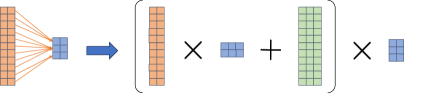
$\mathbf{X}\quad\>\>\>\>\mathbf{X}^{k}\quad\quad\>\>\>\>\>\>\mathbf{X}\mathrm{W}_{\mathbf{Q}}\>\>(\mathbf{X}^{k}\mathrm{W}_{\mathbf{K}})^{\top}\>\>\>\mathrm{H}^{k}\quad\quad\>\>\mathbf{X}^{k}\mathrm{W}_{\mathbf{V}}$

Figure 3: Illustration of our proposed hierarchical global attention.

Hierarchical Global Attention. We propose Hierarchical Graph Transformers with HDSE (HGT-HDSE), a model that uses global attention to capture multi-level structural information in large graphs, defined as

$$\mathbf{X_{A}} =\sum_{k=S}^{K}{\mathrm{softmax}\left(\frac{\mathbf{X}\mathrm{W}_{\mathbf{Q}}(\mathbf{X}^{k}\mathrm{W}_{\mathbf{K}})^{\top}}{\sqrt{d^{\prime}}}+\mathrm{H}^{k}\right)\mathbf{X}^{k}\mathrm{W}_{\mathbf{V}}},$$

$$\mathrm{H}^{k} =\mathrm{Bias}(\mathrm{D}^{k})\in\mathbb{R}^{|V^{0}|\times|V^{k}|},$$ (7)

where parameters $S\geq 1$ is the minimum level of hierarchy, $\mathbf{X}^{k}\in\mathbb{R}^{|V^{k}|\times d}$ (see Sec. 2.1) represents the features of clusters at $k$-level, and $\mathrm{Bias}:\mathbb{R}^{K+1-k}\rightarrow\mathbb{R}$ is a end-to-end trainable function as defined in Sec. 3.2. It is important to note that $|V^{k}|$ is adaptively much smaller than $|V^{0}|$ and can be considered a constant. Therefore, the computation of this hierarchical global attention can be achieved with a time complexity of $O(\sum_{k=S}^{K}{|V^{0}|\times|V^{k}|}\times d)=O(|V^{0}|)$, which is significantly more efficient than the original Transformers (Vaswani et al., 2017) that requires $O(|V^{0}|^{2})$. Our design is simple, scalable, and efficient. It leverages multi-level hierarchical structures to preserve structure-based information and extends the narrow receptive field to overcome over-squashing. Additionally, its capability to focus on far-away node information allows the use of multi-hop features, thereby avoiding over-smoothing.

Incorporation of Local Information. To enhance HGT-HDSE, we incorporate a local module to better process information from the local neighborhood. We employ a straightforward approach that combines $\mathbf{X_{A}}$ with the embeddings produced by GNNs at the output layer:

$$\mathbf{X_{out}}=\mathrm{MLP}((1-\lambda)\mathbf{X_{A}}+\lambda\mathrm{GNN_{G}}(\mathbf{X})),$$ (8)

where $\lambda$ is a weight hyper-parameter, $\mathrm{GNN_{G}}(\mathbf{X})$ is a GNN model with good scalability for large graphs, and $\mathrm{MLP}$ is a projection layer. In the evaluation section, we demonstrate the strong performance of HGT-HDSE in node classification tasks on large-scale graphs.

4 Evaluation

We evaluate our proposed HDSE on 19 benchmark datasets, and show state-of-the-art performance in many cases. Primarily, the following questions are investigated:

• Can HDSE improve upon existing graph transformers, and how does the choice of coarsening algorithm affect performance? (Sec. 4.2)

• Does our HGT-HDSE for large graphs also show effectiveness, is it marked by efficiency, and how does high-level HDSE impact the performance? (Sec. 4.3)

Table 2: Test performance in five benchmarks from (Dwivedi et al., 2023a). Shown is the mean $\pm$ s.d. of 5 runs with different random seeds. Baseline results were obtained from their respective original papers. ^∗ indicates a statistically significant difference against the baseline w/o HDSE from the one-tailed t-test. Highlighted are the top first and second results.

Model	ZINC	MNIST	CIFAR10	PATTERN	CLUSTER
	MAE $\downarrow$	Accuracy $\uparrow$	Accuracy $\uparrow$	Accuracy $\uparrow$	Accuracy $\uparrow$
GCN	0.367 $\pm$ 0.011	90.705 $\pm$ 0.218	55.710 $\pm$ 0.381	71.892 $\pm$ 0.334	68.498 $\pm$ 0.976
GIN	0.526 $\pm$ 0.051	96.485 $\pm$ 0.252	55.255 $\pm$ 1.527	85.387 $\pm$ 0.136	64.716 $\pm$ 1.553
GatedGCN	0.282 $\pm$ 0.015	97.340 $\pm$ 0.143	67.312 $\pm$ 0.311	85.568 $\pm$ 0.088	73.840 $\pm$ 0.326
PNA	0.188 $\pm$ 0.004	97.940 $\pm$ 0.120	70.350 $\pm$ 0.630	–	–
CIN	0.079 $\pm$ 0.006	–	–	–	–
GIN-AK+	0.080 $\pm$ 0.001	–	72.190 $\pm$ 0.130	86.850 $\pm$ 0.057	–
SGFormer	0.306 $\pm$ 0.023	–	–	85.287 $\pm$ 0.097	69.972 $\pm$ 0.634
SAN	0.139 $\pm$ 0.006	–	–	86.581 $\pm$ 0.037	76.691 $\pm$ 0.650
Graphormer	0.122 $\pm$ 0.006	–	–	–	–
Graphormer-GD	0.081 $\pm$ 0.009	–	–	–	–
Specformer	0.066 $\pm$ 0.003	–	–	–	–
EGT	0.108 $\pm$ 0.009	98.173 $\pm$ 0.087	68.702 $\pm$ 0.409	86.821 $\pm$ 0.020	79.232 $\pm$ 0.348
GRIT	0.059 $\pm$ 0.002	98.108 $\pm$ 0.111	76.468 $\pm$ 0.881	87.196 $\pm$ 0.076	80.026 $\pm$ 0.277
GT	0.226 $\pm$ 0.014	90.831 $\pm$ 0.161	59.753 $\pm$ 0.293	84.808 $\pm$ 0.068	73.169 $\pm$ 0.622
GT + HDSE	0.159 $\pm$ 0.006∗	94.394 $\pm$ 0.177∗	64.651 $\pm$ 0.591∗	86.713 $\pm$ 0.049∗	74.223 $\pm$ 0.573∗
SAT	0.094 $\pm$ 0.008	–	–	86.848 $\pm$ 0.037	77.856 $\pm$ 0.104
SAT + HDSE	0.084 $\pm$ 0.003∗	–	–	86.933 $\pm$ 0.039∗	78.513 $\pm$ 0.097∗
GraphGPS	0.070 $\pm$ 0.004	98.051 $\pm$ 0.126	72.298 $\pm$ 0.356	86.685 $\pm$ 0.059	78.016 $\pm$ 0.180
GraphGPS + HDSE	0.062 $\pm$ 0.003∗	98.367 $\pm$ 0.106∗	76.180 $\pm$ 0.277∗	86.737 $\pm$ 0.055	78.498 $\pm$ 0.121∗

Table 3: Test performance on two peptide datasets from Long-Range Graph Benchmarks (LRGB) (Dwivedi et al., 2022).

Model	Peptides-func	Peptides-struct
	AP $\uparrow$	MAE $\downarrow$
GCN	0.5930 $\pm$ 0.0023	0.3496 $\pm$ 0.0013
GINE	0.5498 $\pm$ 0.0079	0.3547 $\pm$ 0.0045
GatedGCN	0.5864 $\pm$ 0.0035	0.3420 $\pm$ 0.0013
GatedGCN+RWSE	0.6069 $\pm$ 0.0035	0.3357 $\pm$ 0.0006
GT	0.6326 $\pm$ 0.0126	0.2529 $\pm$ 0.0016
SAN+LapPE	0.6384 $\pm$ 0.0121	0.2683 $\pm$ 0.0043
SAN+RWSE	0.6439 $\pm$ 0.0075	0.2545 $\pm$ 0.0012
MGT+LapPE	0.6728 $\pm$ 0.0152	0.2488 $\pm$ 0.0014
MGT+RWSE	0.6709 $\pm$ 0.0083	0.2496 $\pm$ 0.0009
GRIT	0.6988 $\pm$ 0.0082	0.2460 $\pm$ 0.0012
GraphGPS	0.6535 $\pm$ 0.0041	0.2500 $\pm$ 0.0012
GraphGPS + HDSE	0.7042 $\pm$ 0.0042∗	0.2457 $\pm$ 0.0013∗

Table 4: Ablations on design choices of coarsening algorithms on ZINC and Peptides-func.

Model	Coarsening	ZINC	Peptides-func
	algorithm	MAE $\downarrow$	AP $\uparrow$
SAT	w/o	0.094 $\pm$ 0.008	–
	METIS	0.089 $\pm$ 0.005	–
	Spectral	0.088 $\pm$ 0.004	–
	Loukas	0.084 $\pm$ 0.003	–
	Newman	0.087 $\pm$ 0.002	–
	Louvain	0.088 $\pm$ 0.003	–
GPS	w/o	0.070 $\pm$ 0.004	0.653 $\pm$ 0.004
	METIS	0.069 $\pm$ 0.002	0.699 $\pm$ 0.003
	Spectral	0.063 $\pm$ 0.003	0.695 $\pm$ 0.004
	Loukas	0.067 $\pm$ 0.002	0.695 $\pm$ 0.010
	Newman	0.062 $\pm$ 0.003	0.704 $\pm$ 0.004
	Louvain	0.064 $\pm$ 0.002	0.699 $\pm$ 0.006

Table 5: Sensitivity analysis on the maximum hierarchy level $K$ of GraphGPS + HDSE on ZINC and Peptides-func.

	$K=0$ (SPD)	$K=1$	$K=2$
ZINC $\downarrow$	0.069 $\pm$ 0.003	0.062 $\pm$ 0.003	0.064 $\pm$ 0.004
P-func $\uparrow$	0.682 $\pm$ 0.009	0.704 $\pm$ 0.004	0.705 $\pm$ 0.006

4.1 Experiment Setting

Datasets. We consider various graph learning tasks from popular benchmarks as detailed below and in Appendix B.

• Graph-level Tasks. For graph classification and regression, we evaluate our method on five datasets from Benchmarking GNNs (Dwivedi et al., 2023a): ZINC, MNIST, CIFAR10, PATTERN, and CLUSTER. We also test on two peptide graph benchmarks from the Long-Range Graph Benchmark (LRGB) (Dwivedi et al., 2022): Peptides-func and Peptides-struct, focusing on classifying graphs into 10 functional classes and regressing 11 structural properties, respectively. We follow all evaluation protocols suggested by (Rampášek et al., 2022).

• Node Classification on Large-scale Graphs. We consider node classification over the citation graphs Cora, CiteSeer and PubMed (Kipf & Welling, 2017), the Actor co-occurrence graph (Chien et al., 2020), and the Squirrel and Chameleon page-page networks from (Rozemberczki et al., 2021), all of which have 1K-20K nodes. Further, we extend our evaluation to larger datasets from the Open Graph Benchmark (OGB) (Hu et al., 2020): ogbn-arxiv, arxiv-year, ogbn-papers100M, and ogbn-proteins, with node numbers ranging from 0.16M to 0.1B. Additionally, we analyze performance on the item co-occurrence network Amazon2M (McAuley et al., 2015) and social network pokec (Leskovec & Krevl, 2016), which have 2.0M and 1.6M nodes, respectively. We maintain all the experimental settings as described in (Wu et al., 2023b).

Baselines. We compare our method to the following prevalent GNNs: GCN (2017), GIN (2018a), GAT (2018), GatedGCN (2017), GatedGCN-RWSE (2021), JKNet (2018b), APPNP (2018), SGC (2019), PNA (2020), GPRGNN (2020), SIGN (2020), H2GCN (2020); and other recent GNNs with SOTA performance: CIN (2021), GIN-AK+ (2021b), HC-GNN (2023). In terms of transformer models, we consider GT(2020), Graphormer (2021), Gophormer (2021a), SAN (2021), Coarformer (2021), ANS-GT (2022), EGT (2022), NodeFormer (2022), Specformer (2023), MGT (2023), AGT (2023b), HSGT (2023), Graphormer-GD (2023), GOAT (2023), Gapformer (2023), LargeGT (2023b) and recent SOTA graph transformers GraphGPS (2022), SAT (2022a), GRIT (2023a), SGFormer (2023b).

Table 6: Node classification on large-scale graphs (%). The baseline results were primarily taken from (Wu et al., 2023b), with the remaining obtained from their respective original papers. OOM indicates out-of-memory when training on a GPU with 24GB memory.

Model	Cora	CiteSeer	PubMed	Actor	Squirrel	Chameleon	ogbn-proteins	ogbn-arxiv	arxiv-year	Amazon2m	pokec	ogbn-100M
# nodes	2,708	3,327	19,717	7,600	2223	890	132,534	169,343	169,343	2,449,029	1,632,803	111,059,956
# edges	5,278	4,552	44,324	29,926	46,998	8,854	39,561,252	1,166,243	1,166,243	61,859,140	30,622,564	1,615,685,872
	Accuracy$\uparrow$	Accuracy$\uparrow$	Accuracy$\uparrow$	Accuracy$\uparrow$	Accuracy$\uparrow$	Accuracy$\uparrow$	ROC-AUC$\uparrow$	Accuracy$\uparrow$	Accuracy$\uparrow$	Accuracy$\uparrow$	Accuracy$\uparrow$	Accuracy$\uparrow$
GCN	81.6 ± 0.4	71.6 ± 0.4	78.8 ± 0.6	30.1 ± 0.2	38.6 ± 1.8	41.3 ± 3.0	72.51 ± 0.35	71.74 ± 0.29	46.02 ± 0.26	83.90 ± 0.10	62.31 ± 1.13	62.04 ± 0.27
GAT	83.0 ± 0.7	72.1 ± 1.1	79.0 ± 0.4	29.8 ± 0.6	35.6 ± 2.1	39.2 ± 3.1	72.02 ± 0.44	71.95 ± 0.36	50.27 ± 0.20	-	-	63.47 ± 0.39
SGC	80.1 ± 0.2	71.9 ± 0.1	78.7 ± 0.1	27.0 ± 0.9	39.3 ± 2.3	39.0 ± 3.3	70.31 ± 0.23	67.79 ± 0.27	-	81.21 ± 0.12	52.03 ± 0.84	63.29 ± 0.19
JKNet	81.8 ± 0.5	70.7 ± 0.7	78.8 ± 0.7	30.8 ± 0.7	39.4 ± 1.6	39.4 ± 3.8	-	72.19 ± 0.21	-	-	-	-
APPNP	83.3 ± 0.5	71.8 ± 0.5	80.1 ± 0.2	31.3 ± 1.5	35.3 ± 1.9	38.4 ± 3.5	-	-	-	-	-	-
SIGN	82.1 ± 0.3	72.4 ± 0.8	79.5 ± 0.5	36.5 ± 1.0	40.7 ± 2.5	41.7 ± 2.2	71.24 ± 0.46	71.95 ± 0.11	-	80.98 ± 0.31	68.01 ± 0.25	65.11 ± 0.14
HC-GNN	81.9 ± 0.4	72.5 ± 0.6	80.2 ± 0.6	-	-	-	-	72.79 ± 0.25	-	-	-	-
Graphormer	75.8 ± 1.1	65.6 ± 0.6	OOM	OOM	40.9 ± 2.5	41.9 ± 2.8	OOM	OOM	OOM	OOM	OOM	OOM
SAT	72.4 ± 0.3	60.9 ± 1.3	OOM	-	-	-	OOM	OOM	OOM	OOM	OOM	OOM
ANS-GT	79.4 ± 0.9	64.5 ± 0.7	77.8 ± 0.7	-	-	-	74.67 ± 0.65	72.34 ± 0.50	-	-	-	-
AGT	81.7 ± 0.4	71.0 ± 0.6	-	-	-	-	-	72.28 ± 0.38	47.38 ± 0.78	-	-	-
HSGT	83.6 ± 1.8	67.4 ± 0.9	79.7 ± 0.5	-	-	-	78.13 ± 0.25	72.58 ± 0.31	-	-	-	-
GraphGPS	76.5 ± 0.6	-	65.7 ± 1.0	33.1 ± 0.8	-	36.2 ± 0.6	-	-	-	-	-	-
GOAT	-	-	75.6 ± 1.2	-	-	-	-	72.41 ± 0.40	53.57 ± 0.18	-	-	61.12 ± 0.10
Gapformer	83.5 ± 0.4	71.4 ± 0.6	80.2 ± 0.4	-	-	-	-	71.90 ± 0.19	-	-	-	-
LargeGT	-	-	-	-	-	-	-	-	-	-	-	64.73 ± 0.05
NodeFormer	82.2 ± 0.9	72.5 ± 1.1	79.9 ± 1.0	36.9 ± 1.0	38.5 ± 1.5	34.7 ± 4.1	77.45 ± 1.15	59.90 ± 0.42	-	87.85 ± 0.24	70.32 ± 0.45	-
SGFormer	84.5 ± 0.8	72.6 ± 0.2	80.3 ± 0.6	37.9 ± 1.1	41.8 ± 2.2	44.9 ± 3.9	79.53 ± 0.38	72.63 ± 0.13	-	89.09 ± 0.10	73.76 ± 0.24	66.01 ± 0.37
HGT-HDSE	83.9 ± 0.7	73.1 ± 0.7	80.6 ± 1.0	38.0 ± 1.5	43.2 ± 2.4	46.0 ± 3.2	80.34 ± 0.32	72.74 ± 0.28	54.23 ± 0.26	89.33 ± 0.15	75.03 ± 0.26	66.04 ± 0.15

Table 7: Efficiency comparison of HGT-HDSE and scalable graph transformer competitors; training time per epoch.

	PubMed	ogbn-arxiv	Amazon2m
GOAT	367.8ms	29.4s	336.2s
NodeFormer	321.4ms	0.6s	5.6s
SGFormer	15.4ms	0.2s	4.8s
HGT-HDSE	13.2ms	0.2s	5.3s

Table 8: Ablation study of the HGT-HDSE modules.

	Actor $\uparrow$	ogbn-proteins $\uparrow$	arxiv-year $\uparrow$
HGT-HDSE	38.0 $\pm$ 1.5	80.3 $\pm$ 0.3	54.2 $\pm$ 0.2
w/o HDSE	34.6 $\pm$ 2.2	79.4 $\pm$ 0.3	53.5 $\pm$ 0.2
w/o GlobAttn	30.1 $\pm$ 0.8	78.1 $\pm$ 0.4	50.9 $\pm$ 0.3

Models + HDSE. We integrate HDSE into Graph Transformer (GT), SAT, GraphGPS (and ANS-GT in appendix) only modifying their self-attention module by Eq. 5. For fair comparisons, we use the same hyperparameters (including the number of layers, batch size, hidden dimension etc.), PE and readout as the baseline transformers. Given one of the baseline transformers M, we denote the modified model using HDSE by M + HDSE. If not specified otherwise, we chose the maximum hierarchy level $K=1$ and maximum distance length $L=30$ in all experiments. During training, the steps of coarsening and distance calculation (Dijkstra, 1959) can be treated as pre-processing, since they only need to be run once. We detail the choice and runtime of coarsening algorithms for HDSE in the appendix. Detailed experimental setup and hyperparameters are in Appendix B due to space constraints.

4.2 Results on Graph-level Tasks

Benchmarks from Benchmarking GNNs, Table 2. We observe that all three baseline graph transformers, when combined with HDSE, demonstrate performance improvements. Note that the enhancement is overall especifally considerable for GT. On CIFAR10, we also obtain similar improvement for GraphGPS. Among them, GT shows the greatest enhancement and becomes competitive to more complex models. Our model attains the best or second-best mean performance for four out of the five datasets, with statistically significant improvements. Notably, it is observed that the SOTA SGFormer tailored for large-scale node classification underperforms in graph-level tasks.

Long-Range Graph Benchmark, Table 3. We consider GraphGPS due to its superior performance. Note that our HDSE module only introduces a small number of additional parameters, allowing it to remain within the benchmark’s $\sim$500k model parameter budget. In the Peptides-func dataset, HDSE yields a significant improvement of 5.07%. This is a promising result and hints at potentially great benefits for macromolecular data more generally.

Impact of Coarsening Algorithms, Table 4, Figure 5. We conduct several ablation experiments on ZINC and Peptides-func and observe that the dependency on the coarsening varies with the dataset and transformer backbone. For instance, the multi-level graph structures extracted by the Newman algorithm yields the largest improvement for GraphGPS. More generally, our experiments indicate that, Newman works best for molecular graphs. We visualize the attention scores on the ZINC and Peptides-func datasets respectively, as shown in Figure 5. The results indicate that our HDSE method successfully leverages hierarchical structure.

Sensitivity Analysis on Hierarchy Level, Table 5. We also conduct a sensitivity analysis on the maximum hierarchy level $K$. The results are shown in Table 5. Note that when $K=0$, HDSE degenerates into SPD, leading to a worse performance. This observation provides empirical evidence to support the effectiveness of our design. Furthermore, as the $K$ increases, there is no significant improvement in the results. This might explain why we chose $K=1$ in line with related works (Zhang et al., 2022; Zhu et al., 2023).

4.3 Results on Large-scale Graphs

Overall Performance, Table 6. We select four categories of baselines: GNNs, graph transformers with proven performance on graph-level tasks, graph transformers with hierarchy, and scalable graph transformers. It’s important to note that, while some graph transformers exhibit superior performance on graph-level tasks, they consistently result in out-of-memory (OOM) in large-scale node tasks. Table 6 demonstrates the competitive performance of our HGT-HDSE, outperforming nearly all other models. In relatively smaller datasets (on the left side), HGT-HDSE shows more significant improvements over baselines, particularly in heterophilic graphs such as Actor, Squirrel, and Chameleon. This could be due to hierarchical global attention filtering out the edges from neighboring nodes of different categories and providing a global perspective enriched with multi-level structural information. Precisely in larger graphs (on the right side), it is the global attention using high-level HDSE that truly surpasses local MPNNs. Across all such larger datasets, HGT-HDSE showcases competitive performance among all baseline methods. This indicates that HGT-HDSE effectively retains global information and is capable of handling the node classification task in such larger graphs. We also observed that all graph transformers with hierarchy suffer from serious overfitting, attributed to their relatively complex architectures. In contrast, HGT-HDSE’s simple architecture contributes to its better generalization.

Efficiency Comparison, Table 7. We report the efficiency results on PubMed, ogbn-arxiv and Amazon2M. It is easy to see that HGT-HDSE outperforms other models in speed, matching the pace of the latest and fastest model, SGFormer (Wu et al., 2023b). It achieves true linear complexity with a streamlined architecture.

Ablation Study, Table 8. To determine the utility of our architectural design choices, we conduct ablation experiments on HGT-HDSE modules over three datasets. The results presented in Table 8, include (1) removing the high-level HDSE and (2) removing the whole global attention module. These experiments reveal a decline in all performance, thereby validating the effectiveness of our architectural design.

5 Conclusions

We have introduced the Hierarchy Distance Structural Encoding (HDSE) method to enhance the capabilities of transformer architectures in graph learning tasks. We have developed a flexible framework to integrate HDSE with various graph transformers and proposed a hierarchical global attention mechanism with linear complexity for applying graph transformers with HDSE to large-scale graphs. Theoretical analysis and empirical results validate the effectiveness and generalization capabilities of HDSE, demonstrating its potential for various real-world applications.

Impact Statements

This paper presents work whose goal is to advance the field of Machine Learning. There are many potential societal consequences of our work, none which we feel must be specifically highlighted here.

Appendix A Proof

Proposition A.1.

(Restatement of Proposition 3.2) GD-WL with HDSE $(\mathrm{D}_{i,j})$ is strictly more expressive than GD-WL with shortest path distances $(\mathrm{SPD}(i,j))$.

Proof.

First, we show that GD-WL with HDSE is at least as expressive as GD-WL with shortest path distances (SPD). Then, we provide a specific example of two graphs that cannot be distinguished by GD-WL with SPD, but can be distinguished by GD-WL with HDSE.

Let $\mathrm{SPD}(i,j)\in\mathbb{R}$ denote the encoding for shortest path distance. It is worth mentioning that

$$\mathrm{D}_{i,j,0}=\mathrm{GHD}^{0}\left(i,j\right)=\mathrm{SPD}\left(i,j\right).$$

Thus, $\mathrm{D}_{i,j}$ is a function of $\mathrm{SPD}\left(i,j\right)$, and hence $\mathrm{D}_{i,j}$ refines $\mathrm{SPD}\left(i,j\right)$. To conclude this, we utilize Lemma 2 from (Bevilacqua et al., 2021), which states that refinement is maintained when using multisets of colors. This observation confirms that GD-WL with HDSE is at least as powerful as GD-WL with SPD.

To show that GD-WL with HDSE is strictly more expressive, we provide an example of two non-isomorphic graphs that can be distinguished by the HDSE but not the SPD: the Desargues graph and the Dodecahedral graph. As depicted in Figure 6 of (Zhang et al., 2023), it has been observed that GD-WL with SPD fails to distinguish these graphs. However, GD-WL with our HDSE can. Figure 4 shows the coarsening results of the Girvan-Newman Algorithm (Girvan & Newman, 2002). We can demonstrate that, for the Dodecahedral graph, each node has $1$-level hierarchy distances of length 2 to other nodes. On the other hand, in the Desargues graph, there are no such distances of length 2 between any pair of nodes. ∎

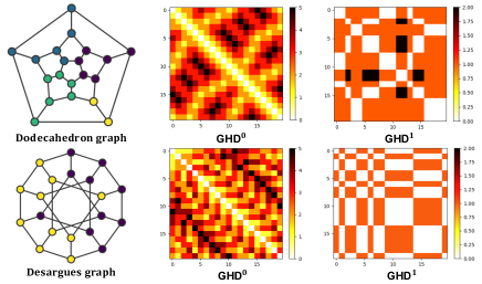
Figure 4: GD-WL with HDSE can distinguish Dodecahedron and Desargues graphs, but GD-WL with SPD cannot.

Proposition A.2.

(Restatement of Corollary 3.3) The power of a graph transformer with HDSE to distinguish non-isomorphic graphs is at most equivalent to that of the GD-WL test with HDSE. With proper parameters and an adequate number of heads and layers, a graph transformer with HDSE can match the power of the GD-WL test with HDSE.

Proof.

The theorem is divided into two parts: the first and second halves. We begin by considering the first half: The power of a graph transformer with HDSE to distinguish non-isomorphic graphs is at most equivalent to that of the GD-WL test with HDSE.

Recall that the GD-WL with HDSE is quite straightforward and can be expressed as:

$$\chi^{t}_{G}(v):=\text{hash}\left\{{(\mathrm{D}_{v,u},\chi^{t-1}_{G}(u)):u\in V}\right\}$$

where $\chi^{t}_{G}(v)$ represents a color mapping function.

Suppose after $t$ iterations, a graph transformer with HDSE $\mathcal{M}$ has $\mathcal{M}(G_{1})\neq\mathcal{M}(G_{2})$, yet GD-WL with HDSE fails to distinguish $G_{1}$ and $G_{2}$ as non-isomorphic. It implies that from iteration 0 to $t$ in the GD-WL test, $G_{1}$ and $G_{2}$ always have the same collection of node labels. Particularly, since $G_{1}$ and $G_{2}$ have the same GD-WL node labels for iterations $i+1$ for any $i=0,\ldots,t-1$, they also share the same collection of GD-WL node labels $\left\{(\mathrm{D}_{v,u},\chi^{i}_{G}(u)):u\in V\right\}$. Otherwise, the GD-WL test would have produced different node labels at iteration $i+1$ for $G_{1}$ and $G_{2}$.

We show that within the same graph, for example $G=G_{1}$, if GD-WL node labels $\chi^{i}_{G}(v)=\chi^{i}_{G}(w)$, then the graph transformer node features $h^{i}_{v}=h^{i}_{w}$ for any iteration $i$. This is clearly true for $i=0$ because GD-WL and graph transformer start with identical node features. Assuming this holds true for iteration $j$, if for any $v,w$, $\chi^{j+1}_{G}(v)=\chi^{j+1}_{G}(w)$, then we must have

$$\left\{(\mathrm{D}_{v,u},\chi^{j}_{G}(u)):u\in V\right\}=\left\{(\mathrm{D}_{w,u},\chi^{j}_{G}(u)):u\in V\right\}.$$

By our assumption at iteration $j$, we deduce that

$$h^{j+1}_{v}={\sum_{u\in V}\mathrm{softmax}(\mathrm{Bias}(\mathrm{D}_{v,u})+h^{j}_{v}\mathbf{W}_{\mathbf{Q}}(h^{j}_{u}\mathbf{W}_{\mathbf{K}})^{\top})h_{u}^{j}\mathbf{W}_{\mathbf{V}}}=\phi(\left\{{(\mathrm{D}_{v,u},\chi^{j}_{G}(u)):u\in V}\right\}).$$

Hence,

$$h^{j+1}_{v}=\phi(\left\{{(\mathrm{D}_{v,u},\chi^{j}_{G}(u)):u\in V}\right\})=\phi(\left\{{(\mathrm{D}_{w,u},\chi^{j}_{G}(u)):u\in V}\right\})=h^{j+1}_{w}.$$

By induction, if GD-WL node labels $\chi^{i}_{G}(v)=\chi^{i}_{G}(w)$, we always have the graph transformer node features $h^{i}_{v}=h^{i}_{w}$ for any iteration $i$. Consequently, from $G_{1}$ and $G_{2}$ having identical GD-WL node labels, it follows that they also have the same graph transformer node features.

Therefore, $h^{i+1}_{v}=h^{i+1}_{w}$. Given that the graph-level readout function is permutation-invariant with respect to the collection of node features, $\mathcal{M}(G_{1})=\mathcal{M}(G_{2})$. This leads to a contradiction.

This completes the proof of the first half of the theorem. For the theorem’s second half, we can entirely leverage the proof of Theorem E.3 by (Zhang et al., 2023) (provided in Appendix E.3), which presents a similar situation.

∎

Proposition A.3.

(Full version of Proposition 3.5) For a semi-supervised binary node classification problem, suppose the label of each node $i\in V$ in the whole graph is determined by the majority vote of discriminative node features in the “hierarchical core neighborhood”: $S_{*}^{i}=\{j:\mathrm{D}_{i,j}=D*\}$ for a certain $D^{*}$, where $\mathrm{D}_{i,j}$ is HDSE defined in (3). Assume noiseless node features. Then, as long as the model is large enough, the batch size $B\geq\Omega(\epsilon^{-2})$, the step size $\eta<1$, the number of iterations $T$ satisfies $T=\Theta(\eta^{-1/2})$ and the number of known labels satisfies $|\mathcal{L}|\geq\max\{\Omega((1+\delta_{D*}^{2})\cdot\log N),BT\}$, where $\delta_{D*}$ measures the maximum number of nodes in the hierarchical core neighborhood $S_{*}^{n}$ for all nodes $n$, then with a probability of at least $0.99$, the returned one-layer graph transformer with HDSE trained by the SGD variant Algorithm 1 and Hinge loss in (Li et al., 2023) can achieve a generalization error which is at most $\epsilon$ for any $\epsilon>0$. However, we do not have a generalization guarantee to learn such a graph characterized by the hierarchical core neighborhood with a one-layer graph transformer with SPD positional encoding.

Before starting the proof, we first briefly introduce and extend some notions and setups used in (Li et al., 2023). The major differences are that (1) we extend their core neighborhood from based on SPD to HDSE (2) we use HDSE in the transformer by encoding it as a one-hot encoding for simplicity of analysis.

Their work focuses on a semi-supervised binary node classification problem on structured graph data, where each node feature corresponds to either a discriminative or a non-discriminative feature, and the dominant discriminative feature in the core neighborhood determines each ground truth node label. For each node, the neighboring nodes with features consistent with the label are called class-relevant nodes, while nodes with features opposite to the label are called confusion nodes. Denote the class-relevant and confusion nodes set for node $n$ as $\mathcal{D}_{*}^{n}$ and $\mathcal{D}_{\#}^{n}$, respectively. A new definition here is the distance-$D$ neighborhood $\mathcal{N}_{D}^{n}$, which is the set of nodes $\{j:\mathrm{D}_{n,j}=D,j\in V\}$. $\mathrm{D}$ is the HDSE defined in (3). Then, by following Definition 1 in (Li et al., 2023), we define the winning margin for each node $n$ of distance $D$ as $\Delta_{n}(D)=|\mathcal{D}_{*}^{n}\cap\mathcal{N}_{D}^{n}|-|\mathcal{D}_{\#}^{n}\cap\mathcal{N}_{D}^{n}|$. The core distance $D*$ is the distance $D$ where the average winning margin over all nodes is the largest. We call the set of neighboring nodes $S_{*}^{n}=\{j:\mathrm{D}_{n,j}=D^{*}\}$ the core neighborhood. We then make the assumption that $\Delta_{n}(D*)>0$ for all nodes $n\in V$, following Assumption 1 in (Li et al., 2023). The one-layer transformer we study is formulated as

$$F(h_{n})=\text{Relu}(\sum_{u\in V}\mathrm{softmax}(\mathrm{B}(\mathrm{D}_{n,u})^{\top}b+h_{n}\mathbf{W}_{\mathbf{Q}}(h_{u}\mathbf{W}_{\mathbf{K}})^{\top})h_{u}\mathbf{W}_{\mathbf{V}}\mathbf{W}_{\mathbf{O}})\boldsymbol{a}$$ (9)

where $\boldsymbol{W}_{O}\in\mathbb{R}^{d^{\prime}\times d^{\prime\prime}}$ and $\boldsymbol{a}\in\mathbb{R}^{d^{\prime\prime}}$ are the hidden and output weights in the two-layer feedforward network, and $b\in\mathbb{R}^{Z}$ is the trainable parameter to learn the positional encoding. The one-hot relative positional encoding $\mathrm{B}(\mathrm{D}_{n,u})$ is defined as

$$\mathrm{B}(\mathrm{D}_{n,u})=\boldsymbol{c}_{s},$$ (10)

where $\boldsymbol{c}_{s}$ is the $s$-th standard basis in $\mathbb{R}^{Z}$. $Z$ is the total number of all possible values of $\mathrm{D}_{n,u}$ for $n,u\in V$. $\mathrm{B}(\cdot)$ is a bijection from $\{d\in\mathbb{R}^{K+1}:d=\mathrm{D}_{n,u}\text{, for certain }n,v\in V\}$ to $\{\boldsymbol{{c}_{1},\boldsymbol{c}_{2},\cdots,\boldsymbol{c}_{Z}}\}$.

Then, we provide the proof for Proposition A.3.

Proof.

The proof follows Theorem 4.1 in (Li et al., 2023) given the above reformulation. Note that (10) can also map the SPD relationship, which is a special one-dimensional case of $\mathrm{D}_{v,u}$, between nodes as (2) in (Li et al., 2023) by the definition of itself. It means that (9) with HDSE can achieve a generalization performance on the graph characterized by the core neighborhood as good as in (Li et al., 2023).

However, we cannot have an inverse conclusion, i.e., providing a generalization guarantee on the graph characterized by the hierarchical core neighborhood using (9) with SPD. This is because SPD cannot distinguish nodes with the same SPD but different HDSE to a certain node. Hence, for a certain node $i\in V$, aggregating nodes using SPD may include nodes outside the hierarchical core neighborhood, of which the labels are inconsistent with the node $i$, and lead to a wrong prediction. ∎

Proposition A.4.

For a semi-supervised binary node classification problem, suppose the label of each node $i\in V$ in the whole graph is determined by the majority vote of discriminative node features in the “core neighborhood”: $S_{*}^{i}=\{j:\mathrm{D}_{i,j}=D*\}$ for a certain $D^{*}$, where $\mathrm{D}_{i,j}$ is HDSE defined in (3). Then, for each node $i\in V$, a properly initialized one-layer graph transformer (i) without HDSE (ii) and only aggregate nodes from $S_{*}^{i}$ can achieve the same generalization error as learning with a one-layer graph transformer (a) with HDSE (b) aggregate all nodes in the graph without knowing $S_{i}^{*}$ in prior.

Proof.

The proof follows Theorem 4.3 in (Li et al., 2023). When $\boldsymbol{b}=0$ is fixed during the training, but the nodes used for training and testing in aggregation for node $n$ are subsets of $\mathcal{N}_{D*}^{n}$, the bound for attention weights on class-relevant nodes is still the same as in (63) and (64) of (Li et al., 2023). Given a known core neighborhood $S_{*}^{n}$, the remaining parameters follow the same order-wise update as Lemmas 4, 5, and 7. The remaining proof steps follow the contents in the proof of Theorem 4.1 of (Li et al., 2023), which leads to a generalization on a one-layer transformer with HDSE and aggregation with all nodes in the graph.

∎

Appendix B Experimental Details

B.1 Computing Environment

Our implementation is based on PyG (Fey & Lenssen, 2019) and DGL (Wang et al., 2019). The experiments are conducted on a single workstation with 4 RTX 3090 GPUs and a quad-core CPU.

Table 9: Overview of the graph learning dataset used in this work (Dwivedi et al., 2023a, 2022; Kipf & Welling, 2017; Chien et al., 2020; Pei et al., 2019; Rozemberczki et al., 2021; Hu et al., 2020; McAuley et al., 2015; Leskovec & Krevl, 2016).

Dataset	# Graphs	Avg. # nodes	Avg. # edges	# Feats	Prediction level	Prediction task	Metric
ZINC	12,000	23.2	24.9	28	graph	regression	MAE
MNIST	70,000	70.6	564.5	3	graph	10-class classif.	Accuracy
CIFAR10	60,000	117.6	941.1	5	graph	10-class classif.	Accuracy
PATTERN	14,000	118.9	3,039.3	3	node	binary classif.	Accuracy
CLUSTER	12,000	117.2	2,150.9	7	node	6-class classif.	Accuracy
Peptides-func	15,535	150.9	307.3	9	graph	10-task classif.	AP
Peptides-struct	15,535	150.9	307.3	9	graph	11-task regression	MAE
Cora	1	2,708	5,278	2,708	node	7-class classif.	Accuracy
Citeseer	1	3,327	4,522	3,703	node	6-class classif.	Accuracy
Pubmed	1	19,717	44,324	500	node	3-class classif.	Accuracy
Actor	1	7,600	26,659	931	node	5-class classif.	Accuracy
Squirrel	1	5,201	216,933	2,089	node	5-class classif.	Accuracy
Chameleon	1	2,277	36,101	2,325	node	5-class classif.	Accuracy
ogbn-proteins	1	132,534	39,561,252	8	node	112 binary classif.	ROC-AUC
ogbn-arxiv	1	169,343	1,166,243	128	node	40-class classif.	Accuracy
arxiv-year	1	169,343	1,166,243	128	node	5-class classif.	Accuracy
Amazon2M	1	2,449,029	61,859,140	100	node	47-class classif.	Accuracy
pokec	1	1,632,803	30,622,564	65	node	binary classif.	Accuracy
ogbn-papers100M	1	111,059,956	1,615,685,872	128	node	172-class classif.	Accuracy

B.2 Description of Datasets

Table 9 presents a summary of the statistics and characteristics of the datasets. The initial five datasets are sourced from (Dwivedi et al., 2023a), followed by two from (Dwivedi et al., 2022), and finally the remaining datasets are obtained from (Kipf & Welling, 2017; Chien et al., 2020; Pei et al., 2019; Rozemberczki et al., 2021; Hu et al., 2020; McAuley et al., 2015; Leskovec & Krevl, 2016).

• ZINC, MNIST, CIFAR10, PATTERN, CLUSTER, Peptides-func and Peptides-struct. For each dataset, we follow the standard train/validation/test splits and evaluation metrics in (Rampášek et al., 2022). For more comprehensive details, readers are encouraged to refer to (Rampášek et al., 2022).

• Cora, Citeseer, Pubmed, Actor, Squirrel, Chameleon, ogbn-proteins, ogbn-arxiv, Amazon2M, pokec and ogbn-papers100M. For each dataset, we use the same train/validation/test splits and evaluation metrics as (Wu et al., 2023b). For detailed information on these datasets, please refer to (Wu et al., 2023b).

• Arxiv-year is a citation network among all computer science arxiv papers, as described by (Lim et al., 2021). In this network, each node corresponds to an arxiv paper, and the edges indicate the citations between papers. Each paper is associated with a 128-dimensional feature vector, obtained by averaging the word embeddings of its title and abstract. The word embeddings are generated using the WORD2VEC model. The labels of arxiv-year are publication years clustered into fve intervals. We use the public splits shared by (Lim et al., 2021), with a train/validation/test split ratio of 50%/25%/25%.

Table 10: Hyperparameters of GraphGPS + HDSE for five datasets from (Dwivedi et al., 2023a).

Hyperparameter	ZINC	MNIST	CIFAR10	PATTERN	CLUSTER
# GPS Layers	10	3	3	6	16
Hidden dim	64	52	52	64	48
GPS-MPNN	GINE	GatedGCN	GatedGCN	GatedGCN	GatedGCN
GPS-GlobAttn	Transformer	Transformer	Transformer	Transformer	Transformer
# Heads	4	4	4	4	8
Attention dropout	0.5	0.5	0.5	0.5	0.5
Graph pooling	sum	mean	mean	–	–
Positional Encoding	RWSE-20	LapPE-8	LapPE-8	LapPE-16	LapPE-10
PE dim	28	8	8	16	16
PE encoder	linear	DeepSet	DeepSet	DeepSet	DeepSet
Batch size	32	16	16	32	16
Learning Rate	0.001	0.001	0.001	0.0005	0.0005
# Epochs	2000	100	200	100	100
# Warmup epochs	50	5	5	5	5
Weight decay	1e-5	1e-5	1e-5	1e-5	1e-5
Coarsening algorithm	Newman	Louvain	Louvain	Loukas ($\alpha=0.1$)	Louvain
# Parameters	437,389	124,565	121,913	352,695	517,446

Table 11: Hyperparameters of GraphGPS + HDSE for two LRGB datasets from (Dwivedi et al., 2022).

Hyperparameter	Peptides-func	Peptides-struct
# GPS Layers	4	4
Hidden dim	96	96
GPS-MPNN	GatedGCN	GatedGCN
GPS-GlobAttn	Transformer	Transformer
# Heads	4	4
Attention dropout	0.5	0.5
Graph pooling	mean	mean
Positional Encoding	LapPE-10	LapPE-10
PE dim	16	16
PE encoder	DeepSet	DeepSet
Batch size	16	128
Learning Rate	0.0003	0.0003
# Epochs	200	200
# Warmup epochs	5	5
Weight decay	0	0
Coarsening algorithm	Newman	METIS ($\alpha=0.1$)
# Parameters	505,866	506,235

B.3 Hyperparameter and Reproducibility

Models + HDSE. For fair comparisons, we use the same hyperparameters (including training schemes, optimizer, number of layers, batch size, hidden dimension etc.) as baseline models for all of our HDSE versions. Taking GraphGPS + HDSE as an example, Tables 10 and 11 showcase the corresponding hyperparameters and coarsening algorithms. It is important to note that our HDSE module introduces only a small number of additional parameters.

HGT-HDSE Configurations. For the hyperparameter selections of our HGT-HDSE model, in addition to what we have covered in the setting part of the experiment section that datasets share in common, we list other settings in Table 12. It’s important to note that our hyperparameters were determined within the SGFormer’s grid search space. Furthermore, all other experimental parameters, including dropout, batch size, training schemes, optimizer, etc., are consistent with those used in the SGFormer (Wu et al., 2019). The testing accuracy achieved by the model that reports the highest result on the validation set is used for evaluation. And each experiment is repeated 10 times to get the mean value and error bar.

SGFormer on Graph-level Tasks. To accurately demonstrate the capabilities of SGFormer on these datasets, we use all the same experimental settings and conduct the same grid search as outlined in GraphGPS (Rampášek et al., 2022).

Table 12: HGT-HDSE dataset-specific hyperparameter settings.

Dataset	$|V^{1}|$	Hidden dim	# Heads	# Glob. Layers	GNN	# GNN Layers	$\lambda$	# Epochs	LR
Cora	256	128	1	1	GCN	2	0.8	500	1e-2
Citeseer	256	128	1	1	GCN	2	0.5	500	1e-2
Pubmed	32	128	4	2	GCN	2	0.8	500	1e-2
Actor	200	128	2	1	GCN	2	0.0	1000	1e-2
Squirrel	128	128	1	3	GCN	2	0.2	500	1e-2
Chameleon	32	128	1	3	GCN	2	0.5	500	1e-2
ogbn-proteins	1024	128	2	1	GraphSAGE	4	0.5	1000	5e-4
ogbn-arxiv	1024	256	1	3	GCN	3	0.5	1000	1e-2
arxiv-year	2048	128	4	1	GAT	1	0.5	500	1e-3
Amazon2M	1024	256	1	1	GCN	3	0.5	1000	1e-2
pokec	1024	64	1	3	GCN	2	0.5	1000	1e-2
ogbn-papers100M	1024	256	1	1	GCN	3	0.5	50	1e-3

Appendix C Additional Experimental Results

C.1 Coarsening Runtime

Table 13 gives the runtime of coarsening algorithms (including distance calculation) on graph-level tasks, illustrating the practicality of our method. The Newman algorithm is unsuited for larger graphs due to high complexity. In addition, our HDSE module almost does not increase the runtime of the baselines. For example, GraphGPS runs at 10 seconds per epoch, compared to 11 seconds per epoch with HDSE module on ZINC.

Additionally, for all large-scale graphs, we employ METIS due to its efficiency with a time complexity of $O(|E|)$. This makes it highly effective for partitioning extensive graphs, such as Amazon2M, in less than 5 minutes, and even the vast ogbn-papers100M, with a size of 0.1 billion nodes, requires only 59 minutes.

Table 13: Empirical runtime of coarsening algorithms.

Algorithm	ZINC	PATTERN	MNIST	P-func
METIS	31s	0.1h	0.2h	0.1h
Newman	88s	$>$500h	18h	1.6h
Louvain	76s	5h	1.6h	1.1h

Table 14: Node classification on synthetic community datasets.

Dataset	GT	GT + SPD	GT + HDSE
Community-small	64.7 $\pm$ 1.1	81.5 $\pm$ 1.7	88.6 $\pm$ 0.9

C.2 Synthetic Community Dataset

We evaluate the Community-small dataset from GraphRNN (You et al., 2018), a synthetic dataset featuring community structures. It comprises 100 graphs, each with two distinct communities. These communities are generated using the Erdos-Renyi model (E-R). Node features are generated from random numbers and node labels are determined by their respective cluster numbers with accuracy as the chosen evaluation metric. We use the a random train/validation/test split ratio of 60%/20%/20%.

We select the Louvain method as our coarsening algorithm and integrate the HDSE module into the Graph Transformer (GT). As shown in Table 14, the GT struggles to detect such structures; and solely utilizing SPD proves inadequate; however, our HDSE, enriched with coarsening structural information, effectively captures these structures.

C.3 ANS-GT + HDSE

We validate the performance of our HDSE framework using the efficient ANS-GT (Zhang et al., 2022), which uses a multi-armed bandit algorithm to adaptively sample nodes for attention. We use the Louvain method as our coarsening algorithm. And for each pair of nodes sampled adaptively by the ANS-GT, we calculate their HDSE and bias the attention computation. For fair comparisons, we tune the hyperparameters using the same grid search as reported in their paper (Zhang et al., 2022). Note that we report the supervised learning setting (different from the text), since this is the one considered in the ANS-GT (Zhang et al., 2022). Overall, Table 15 shows that HDSE yields consistent performance improvements, even in this challenging scenario, where nodes are sampled.

Table 15: Node classification accuracy on ANS-GT + HDSE (%). The baseline results were taken from (Zhang et al., 2022). We apply 3 independent runs on random data splitting. ⁺ indicates the results obtained from our re-running.

Model	Cora	Citeseer	Pubmed
GCN	87.33 $\pm$ 0.38	79.43 $\pm$ 0.26	84.86 $\pm$ 0.19
GAT	86.29 $\pm$ 0.53	80.13 $\pm$ 0.62	84.40 $\pm$ 0.05
APPNP	87.15 $\pm$ 0.43	79.33 $\pm$ 0.35	87.04 $\pm$ 0.17
JKNet	87.70 $\pm$ 0.65	78.43 $\pm$ 0.31	87.64 $\pm$ 0.26
H2GCN	87.92 $\pm$ 0.82	77.60 $\pm$ 0.76	89.55 $\pm$ 0.14
GPRGNN	88.27 $\pm$ 0.40	78.46 $\pm$ 0.88	89.38 $\pm$ 0.43
GT	71.84 $\pm$ 0.62	67.38 $\pm$ 0.76	82.11 $\pm$ 0.39
SAN	74.02 $\pm$ 1.01	70.64 $\pm$ 0.97	86.22 $\pm$ 0.43
Graphormer	72.85 $\pm$ 0.76	66.21 $\pm$ 0.83	82.76 $\pm$ 0.24
Gophormer	87.65 $\pm$ 0.20	76.43 $\pm$ 0.78	88.33 $\pm$ 0.44
Coarformer	88.69 $\pm$ 0.82	79.20 $\pm$ 0.89	89.75 $\pm$ 0.31
ANS-GT	88.60 $\pm$ 0.45	77.75 $\pm$ 0.79+	89.56 $\pm$ 0.55
ANS-GT + HDSE	89.67 $\pm$ 0.39	78.31 $\pm$ 0.58	90.63 $\pm$ 0.26

C.4 Clustering Coefficients Analysis

We check if there is a correlation with the cluster structure according to (Hu et al., 2020), by computing clustering coefficients on five benchmarks from (Dwivedi et al., 2023a), but we do not observe a direct correlation. Notably, the ZINC dataset, which comprises small molecules, has a low clustering coefficient; however, our HDSE shows a significant improvement on it. This improvement could be attributed to the HDSE capturing chemical motifs that cannot be captured by the clustering coefficient, as illustrated in Figure 2.

Table 16: Clustering Coefficients Analysis.

Model	ZINC	MNIST	CIFAR10	PATTERN	CLUSTER
	MAE $\downarrow$	Accuracy $\uparrow$	Accuracy $\uparrow$	Accuracy $\uparrow$	Accuracy $\uparrow$
Average Clust. Coeff.	0.006	0.477	0.454	0.427	0.316
GT	0.226 $\pm$ 0.014	90.831 $\pm$ 0.161	59.753 $\pm$ 0.293	84.808 $\pm$ 0.068	73.169 $\pm$ 0.622
GT + HDSE	0.159 $\pm$ 0.006	94.394 $\pm$ 0.177	64.651 $\pm$ 0.591	86.713 $\pm$ 0.049	74.223 $\pm$ 0.573
SAT	0.094 $\pm$ 0.008	–	–	86.848 $\pm$ 0.037	77.856 $\pm$ 0.104
SAT + HDSE	0.084 $\pm$ 0.003	–	–	86.933 $\pm$ 0.039	78.513 $\pm$ 0.097
GraphGPS	0.070 $\pm$ 0.004	98.051 $\pm$ 0.126	72.298 $\pm$ 0.356	86.685 $\pm$ 0.059	78.016 $\pm$ 0.180
GraphGPS + HDSE	0.062 $\pm$ 0.003	98.367 $\pm$ 0.106	76.180 $\pm$ 0.277	86.737 $\pm$ 0.055	78.498 $\pm$ 0.121

Appendix D HDSE Visualization

Here, we demonstrate that our HDSE method also provides interpretability compared to the classic GT. We train the GT + HDSE and GT on ZINC and Peptides-func graphs, and compare the attention scores between the selected node and other nodes. Figure 5 visualizes the attention scores on ZINC and Peptides-func. The results indicate that, after integrating the HDSE bias, the attention mechanism tends to focus on certain community structures rather than individual nodes as seen in classic attention. This phenomenon demonstrates our method’s capacity to capture multi-level hierarchical structures.

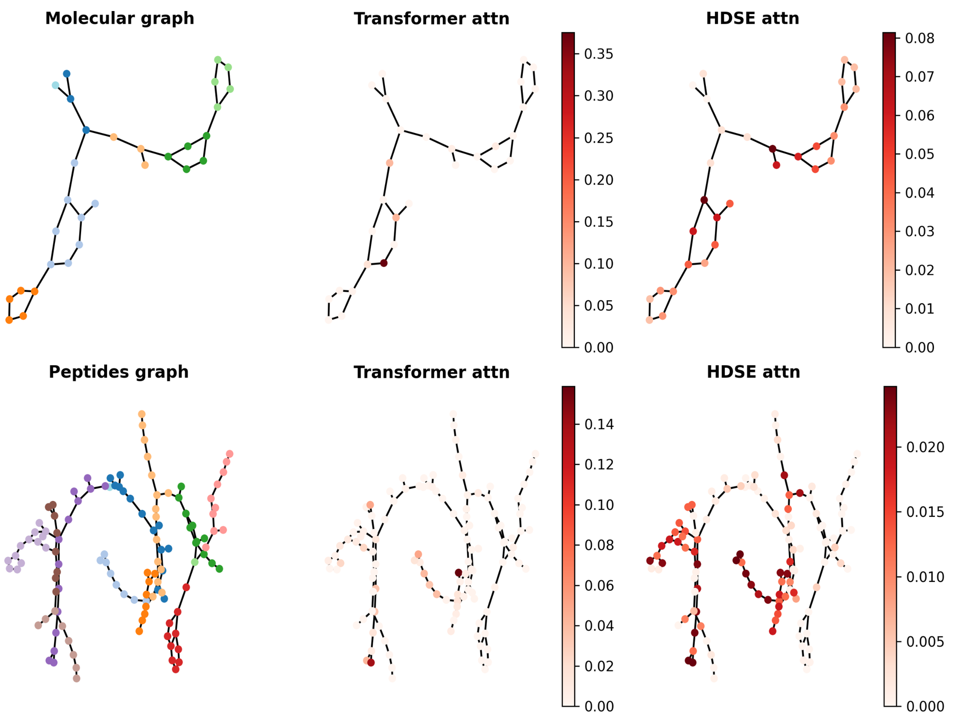
Figure 5: Visualization of attention weights for the transformer attention and HDSE attention. The left side illustrates the graph coarsening result. The center column displays the attention weights of a sample node learned by the classic GT (Dwivedi & Bresson, 2020), while the right column showcases the attention weights learned by the HDSE attention.

Appendix E Further Related Works

Graph Transformers over Clustering Pooling. Kong et al. (2023) employs a hybrid approach that integrates a neighbor-sampling local module with a global module, the latter featuring a trainable, fixed-size codebook obtained by K-Means to represent global centroids, which is noted for its efficiency. Meanwhile, Gapformer (Liu et al., 2023) involves the incorporation of a graph pooling layer designed to refine the key and value matrices into pooled key and value vectors through graph pooling operations. This approach aims to minimize the presence of irrelevant nodes and reduce computational demands. However, the performance of these methods remains constrained due to a lack of effective inductive biases.

Graph Transformers over Virtual Nodes. Several graph transformer models utilize anchor nodes or virtual nodes for message propagation. For instance, Graphormer (Ying et al., 2021) introduces a virtual node and establishes connections between the virtual node and each individual node. AGFormer (Jiang et al., 2023) selects representative anchors and transforms node-to-node message passing into an anchor-to-anchor and anchor-to-node message passing process. Additionally, AGT (Ma et al., 2023b) extracts structural patterns from subgraph views and designs an adaptive transformer block to dynamically integrate attention scores in a node-specific manner.

References

- Alon & Yahav (2020) Alon, U. and Yahav, E. On the bottleneck of graph neural networks and its practical implications. arXiv preprint arXiv:2006.05205, 2020.
- Bai et al. (2022) Bai, L., Cui, L., and Edwin, H. A hierarchical transitive-aligned graph kernel for un-attributed graphs. In International Conference on Machine Learning, pp. 1327–1336. PMLR, 2022.
- Bevilacqua et al. (2021) Bevilacqua, B., Frasca, F., Lim, D., Srinivasan, B., Cai, C., Balamurugan, G., Bronstein, M. M., and Maron, H. Equivariant subgraph aggregation networks. arXiv preprint arXiv:2110.02910, 2021.
- Bianchi et al. (2020) Bianchi, F. M., Grattarola, D., and Alippi, C. Spectral clustering with graph neural networks for graph pooling. In International conference on machine learning, pp. 874–883. PMLR, 2020.
- Blondel et al. (2008) Blondel, V. D., Guillaume, J.-L., Lambiotte, R., and Lefebvre, E. Fast unfolding of communities in large networks. Journal of statistical mechanics: theory and experiment, 2008(10):P10008, 2008.
- Bo et al. (2023) Bo, D., Shi, C., Wang, L., and Liao, R. Specformer: Spectral graph neural networks meet transformers. arXiv preprint arXiv:2303.01028, 2023.
- Bodnar et al. (2021) Bodnar, C., Frasca, F., Wang, Y., Otter, N., Montufar, G. F., Lio, P., and Bronstein, M. Weisfeiler and lehman go topological: Message passing simplicial networks. In International Conference on Machine Learning, pp. 1026–1037. PMLR, 2021.
- Bresson & Laurent (2017) Bresson, X. and Laurent, T. Residual gated graph convnets. arXiv preprint arXiv:1711.07553, 2017.
- Bronstein et al. (2021) Bronstein, M. M., Bruna, J., Cohen, T., and Veličković, P. Geometric deep learning: Grids, groups, graphs, geodesics, and gauges. arXiv preprint arXiv:2104.13478, 2021.
- Chen et al. (2022a) Chen, D., O’Bray, L., and Borgwardt, K. Structure-aware transformer for graph representation learning. In International Conference on Machine Learning, pp. 3469–3489. PMLR, 2022a.
- Chen et al. (2022b) Chen, J., Gao, K., Li, G., and He, K. Nagphormer: A tokenized graph transformer for node classification in large graphs. In The Eleventh International Conference on Learning Representations, 2022b.
- Chien et al. (2020) Chien, E., Peng, J., Li, P., and Milenkovic, O. Adaptive universal generalized pagerank graph neural network. In International Conference on Learning Representations, 2020.
- Corso et al. (2020) Corso, G., Cavalleri, L., Beaini, D., Liò, P., and Veličković, P. Principal neighbourhood aggregation for graph nets. Advances in Neural Information Processing Systems, 33:13260–13271, 2020.
- Dijkstra (1959) Dijkstra, E. A note on two problems in connexion with graphs. Numerische Mathematik, 1(1):269–271, 1959.
- Dosovitskiy et al. (2020) Dosovitskiy, A., Beyer, L., Kolesnikov, A., Weissenborn, D., Zhai, X., Unterthiner, T., Dehghani, M., Minderer, M., Heigold, G., Gelly, S., et al. An image is worth 16x16 words: Transformers for image recognition at scale. In International Conference on Learning Representations, 2020.
- Dwivedi & Bresson (2020) Dwivedi, V. P. and Bresson, X. A generalization of transformer networks to graphs. arXiv preprint arXiv:2012.09699, 2020.
- Dwivedi et al. (2021) Dwivedi, V. P., Luu, A. T., Laurent, T., Bengio, Y., and Bresson, X. Graph neural networks with learnable structural and positional representations. In International Conference on Learning Representations, 2021.
- Dwivedi et al. (2022) Dwivedi, V. P., Rampášek, L., Galkin, M., Parviz, A., Wolf, G., Luu, A. T., and Beaini, D. Long range graph benchmark. arXiv preprint arXiv:2206.08164, 2022.
- Dwivedi et al. (2023a) Dwivedi, V. P., Joshi, C. K., Luu, A. T., Laurent, T., Bengio, Y., and Bresson, X. Benchmarking graph neural networks. Journal of Machine Learning Research, 24(43):1–48, 2023a.
- Dwivedi et al. (2023b) Dwivedi, V. P., Liu, Y., Luu, A. T., Bresson, X., Shah, N., and Zhao, T. Graph transformers for large graphs. arXiv preprint arXiv:2312.11109, 2023b.
- Fey & Lenssen (2019) Fey, M. and Lenssen, J. E. Fast graph representation learning with pytorch geometric. arXiv preprint arXiv:1903.02428, 2019.
- Gao & Ji (2019) Gao, H. and Ji, S. Graph u-nets. In international conference on machine learning, pp. 2083–2092. PMLR, 2019.
- Gao et al. (2022) Gao, H., Han, X., Huang, J., Wang, J.-X., and Liu, L. Patchgt: Transformer over non-trainable clusters for learning graph representations. In Learning on Graphs Conference, pp. 27–1. PMLR, 2022.
- Gasteiger et al. (2018) Gasteiger, J., Bojchevski, A., and Günnemann, S. Predict then propagate: Graph neural networks meet personalized pagerank. arXiv preprint arXiv:1810.05997, 2018.
- Gilmer et al. (2017) Gilmer, J., Schoenholz, S. S., Riley, P. F., Vinyals, O., and Dahl, G. E. Neural message passing for quantum chemistry. In International conference on machine learning, pp. 1263–1272. PMLR, 2017.
- Girvan & Newman (2002) Girvan, M. and Newman, M. E. Community structure in social and biological networks. Proceedings of the national academy of sciences, 99(12):7821–7826, 2002.
- Hu et al. (2020) Hu, W., Fey, M., Zitnik, M., Dong, Y., Ren, H., Liu, B., Catasta, M., and Leskovec, J. Open graph benchmark: Datasets for machine learning on graphs. Advances in neural information processing systems, 33:22118–22133, 2020.
- Huang et al. (2019) Huang, J., Li, Z., Li, N., Liu, S., and Li, G. Attpool: Towards hierarchical feature representation in graph convolutional networks via attention mechanism. In Proceedings of the IEEE/CVF international conference on computer vision, pp. 6480–6489, 2019.
- Hussain et al. (2022) Hussain, M. S., Zaki, M. J., and Subramanian, D. Global self-attention as a replacement for graph convolution. In Proceedings of the 28th ACM SIGKDD Conference on Knowledge Discovery and Data Mining, pp. 655–665, 2022.
- Hwang et al. (2022) Hwang, E., Thost, V., Dasgupta, S. S., and Ma, T. An analysis of virtual nodes in graph neural networks for link prediction (extended abstract). In The First Learning on Graphs Conference, 2022. URL https://openreview.net/forum?id=dI6KBKNRp7.
- Jiang et al. (2023) Jiang, B., Xu, F., Zhang, Z., Tang, J., and Nie, F. Agformer: Efficient graph representation with anchor-graph transformer. arXiv preprint arXiv:2305.07521, 2023.
- Jin et al. (2020) Jin, W., Barzilay, R., and Jaakkola, T. Hierarchical generation of molecular graphs using structural motifs. In International conference on machine learning, pp. 4839–4848. PMLR, 2020.
- Karypis & Kumar (1998) Karypis, G. and Kumar, V. A software package for partitioning unstructured graphs, partitioning meshes, and computing fill-reducing orderings of sparse matrices. University of Minnesota, Department of Computer Science and Engineering, Army HPC Research Center, Minneapolis, MN, 38:7–1, 1998.
- Kipf & Welling (2017) Kipf, T. N. and Welling, M. Semi-supervised classification with graph convolutional networks. In International Conference on Learning Representations, 2017. URL https://openreview.net/forum?id=SJU4ayYgl.
- Kong et al. (2023) Kong, K., Chen, J., Kirchenbauer, J., Ni, R., Bruss, C. B., and Goldstein, T. GOAT: A global transformer on large-scale graphs. In Krause, A., Brunskill, E., Cho, K., Engelhardt, B., Sabato, S., and Scarlett, J. (eds.), Proceedings of the 40th International Conference on Machine Learning, volume 202 of Proceedings of Machine Learning Research, pp. 17375–17390. PMLR, 23–29 Jul 2023. URL https://proceedings.mlr.press/v202/kong23a.html.
- Kreuzer et al. (2021) Kreuzer, D., Beaini, D., Hamilton, W., Létourneau, V., and Tossou, P. Rethinking graph transformers with spectral attention. Advances in Neural Information Processing Systems, 34:21618–21629, 2021.
- Kuang et al. (2021) Kuang, W., Zhen, W., Li, Y., Wei, Z., and Ding, B. Coarformer: Transformer for large graph via graph coarsening. 2021.
- Lee et al. (2019) Lee, J., Lee, I., and Kang, J. Self-attention graph pooling. In International conference on machine learning, pp. 3734–3743. PMLR, 2019.
- Leskovec & Krevl (2016) Leskovec, J. and Krevl, A. Snap datasets: Stanford large network dataset collection. 2014. 2016.
- Li et al. (2023) Li, H., Wang, M., Ma, T., Liu, S., ZHANG, Z., and Chen, P.-Y. What improves the generalization of graph transformer? a theoretical dive into self-attention and positional encoding. In NeurIPS 2023 Workshop: New Frontiers in Graph Learning, 2023. URL https://openreview.net/forum?id=BaxFC3z9R6.
- Li et al. (2018) Li, Y., Vinyals, O., Dyer, C., Pascanu, R., and Battaglia, P. Learning deep generative models of graphs. arXiv preprint arXiv:1803.03324, 2018.
- Lim et al. (2021) Lim, D., Hohne, F., Li, X., Huang, S. L., Gupta, V., Bhalerao, O., and Lim, S. N. Large scale learning on non-homophilous graphs: New benchmarks and strong simple methods. Advances in Neural Information Processing Systems, 34:20887–20902, 2021.
- Liu et al. (2023) Liu, C., Zhan, Y., Ma, X., Ding, L., Tao, D., Wu, J., and Hu, W. Gapformer: Graph transformer with graph pooling for node classification. In Proceedings of the Thirty-Second International Joint Conference on Artificial Intelligence, IJCAI, pp. 2196–2205, 2023.
- Loukas (2019) Loukas, A. Graph reduction with spectral and cut guarantees. J. Mach. Learn. Res., 20(116):1–42, 2019.
- Ma et al. (2023a) Ma, L., Lin, C., Lim, D., Romero-Soriano, A., Dokania, P. K., Coates, M., Torr, P., and Lim, S.-N. Graph inductive biases in transformers without message passing. arXiv preprint arXiv:2305.17589, 2023a.
- Ma et al. (2023b) Ma, X., Chen, Q., Wu, Y., Song, G., Wang, L., and Zheng, B. Rethinking structural encodings: Adaptive graph transformer for node classification task. In Proceedings of the ACM Web Conference 2023, pp. 533–544, 2023b.
- McAuley et al. (2015) McAuley, J., Pandey, R., and Leskovec, J. Inferring networks of substitutable and complementary products. In Proceedings of the 21th ACM SIGKDD international conference on knowledge discovery and data mining, pp. 785–794, 2015.
- Min et al. (2022) Min, E., Chen, R., Bian, Y., Xu, T., Zhao, K., Huang, W., Zhao, P., Huang, J., Ananiadou, S., and Rong, Y. Transformer for graphs: An overview from architecture perspective. arXiv preprint arXiv:2202.08455, 2022.
- Ng et al. (2001) Ng, A., Jordan, M., and Weiss, Y. On spectral clustering: Analysis and an algorithm. Advances in neural information processing systems, 14, 2001.
- Ngo et al. (2023) Ngo, N. K., Hy, T. S., and Kondor, R. Multiresolution graph transformers and wavelet positional encoding for learning long-range and hierarchical structures. The Journal of Chemical Physics, 159(3), 2023.
- Pei et al. (2019) Pei, H., Wei, B., Chang, K. C.-C., Lei, Y., and Yang, B. Geom-gcn: Geometric graph convolutional networks. In International Conference on Learning Representations, 2019.
- Rampášek et al. (2022) Rampášek, L., Galkin, M., Dwivedi, V. P., Luu, A. T., Wolf, G., and Beaini, D. Recipe for a general, powerful, scalable graph transformer. arXiv preprint arXiv:2205.12454, 2022.
- Ranjan et al. (2020) Ranjan, E., Sanyal, S., and Talukdar, P. Asap: Adaptive structure aware pooling for learning hierarchical graph representations. In Proceedings of the AAAI Conference on Artificial Intelligence, volume 34, pp. 5470–5477, 2020.
- Rossi et al. (2020) Rossi, E., Frasca, F., Chamberlain, B., Eynard, D., Bronstein, M., and Monti, F. Sign: Scalable inception graph neural networks. arXiv preprint arXiv:2004.11198, 7:15, 2020.
- Rozemberczki et al. (2021) Rozemberczki, B., Allen, C., and Sarkar, R. Multi-scale attributed node embedding. Journal of Complex Networks, 9(2):cnab014, 2021.
- Shirzad et al. (2023) Shirzad, H., Velingker, A., Venkatachalam, B., Sutherland, D. J., and Sinop, A. K. Exphormer: Sparse transformers for graphs. arXiv preprint arXiv:2303.06147, 2023.
- Topping et al. (2021) Topping, J., Di Giovanni, F., Chamberlain, B. P., Dong, X., and Bronstein, M. M. Understanding over-squashing and bottlenecks on graphs via curvature. arXiv preprint arXiv:2111.14522, 2021.
- Vaswani et al. (2017) Vaswani, A., Shazeer, N., Parmar, N., Uszkoreit, J., Jones, L., Gomez, A. N., Kaiser, L., and Polosukhin, I. Attention is all you need. Advances in neural information processing systems, 30, 2017.
- Veličković et al. (2018) Veličković, P., Cucurull, G., Casanova, A., Romero, A., Liò, P., and Bengio, Y. Graph attention networks. In International Conference on Learning Representations, 2018.
- Wang et al. (2019) Wang, M., Zheng, D., Ye, Z., Gan, Q., Li, M., Song, X., Zhou, J., Ma, C., Yu, L., Gai, Y., et al. Deep graph library: A graph-centric, highly-performant package for graph neural networks. arXiv preprint arXiv:1909.01315, 2019.
- Weisfeiler & Leman (1968) Weisfeiler, B. and Leman, A. The reduction of a graph to canonical form and the algebra which appears therein. nti, Series, 2(9):12–16, 1968.
- Wu et al. (2019) Wu, F., Souza, A., Zhang, T., Fifty, C., Yu, T., and Weinberger, K. Simplifying graph convolutional networks. In International conference on machine learning, pp. 6861–6871. PMLR, 2019.
- Wu et al. (2022) Wu, Q., Zhao, W., Li, Z., Wipf, D. P., and Yan, J. Nodeformer: A scalable graph structure learning transformer for node classification. Advances in Neural Information Processing Systems, 35:27387–27401, 2022.
- Wu et al. (2023a) Wu, Q., Yang, C., Zhao, W., He, Y., Wipf, D., and Yan, J. DIFFormer: Scalable (graph) transformers induced by energy constrained diffusion. In The Eleventh International Conference on Learning Representations, 2023a. URL https://openreview.net/forum?id=j6zUzrapY3L.
- Wu et al. (2023b) Wu, Q., Zhao, W., Yang, C., Zhang, H., Nie, F., Jiang, H., Bian, Y., and Yan, J. Simplifying and empowering transformers for large-graph representations. In Thirty-seventh Conference on Neural Information Processing Systems, 2023b. URL https://openreview.net/forum?id=R4xpvDTWkV.
- Xu et al. (2018a) Xu, K., Hu, W., Leskovec, J., and Jegelka, S. How powerful are graph neural networks? arXiv preprint arXiv:1810.00826, 2018a.
- Xu et al. (2018b) Xu, K., Li, C., Tian, Y., Sonobe, T., Kawarabayashi, K.-i., and Jegelka, S. Representation learning on graphs with jumping knowledge networks. In International conference on machine learning, pp. 5453–5462. PMLR, 2018b.
- Ying et al. (2021) Ying, C., Cai, T., Luo, S., Zheng, S., Ke, G., He, D., Shen, Y., and Liu, T.-Y. Do transformers really perform badly for graph representation? Advances in Neural Information Processing Systems, 34:28877–28888, 2021.
- Ying et al. (2018) Ying, Z., You, J., Morris, C., Ren, X., Hamilton, W., and Leskovec, J. Hierarchical graph representation learning with differentiable pooling. Advances in neural information processing systems, 31, 2018.
- You et al. (2018) You, J., Ying, R., Ren, X., Hamilton, W., and Leskovec, J. Graphrnn: Generating realistic graphs with deep auto-regressive models. In International conference on machine learning, pp. 5708–5717. PMLR, 2018.
- Zhang et al. (2023) Zhang, B., Luo, S., Wang, L., and He, D. Rethinking the expressive power of GNNs via graph biconnectivity. In The Eleventh International Conference on Learning Representations, 2023. URL https://openreview.net/forum?id=r9hNv76KoT3.
- Zhang et al. (2022) Zhang, Z., Liu, Q., Hu, Q., and Lee, C.-K. Hierarchical graph transformer with adaptive node sampling. Advances in Neural Information Processing Systems, 35:21171–21183, 2022.
- Zhao et al. (2021a) Zhao, J., Li, C., Wen, Q., Wang, Y., Liu, Y., Sun, H., Xie, X., and Ye, Y. Gophormer: Ego-graph transformer for node classification. arXiv preprint arXiv:2110.13094, 2021a.
- Zhao et al. (2021b) Zhao, L., Jin, W., Akoglu, L., and Shah, N. From stars to subgraphs: Uplifting any gnn with local structure awareness. arXiv preprint arXiv:2110.03753, 2021b.
- Zhong et al. (2023) Zhong, Z., Li, C.-T., and Pang, J. Hierarchical message-passing graph neural networks. Data Mining and Knowledge Discovery, 37(1):381–408, 2023.
- Zhu et al. (2020) Zhu, J., Yan, Y., Zhao, L., Heimann, M., Akoglu, L., and Koutra, D. Beyond homophily in graph neural networks: Current limitations and effective designs. Advances in neural information processing systems, 33:7793–7804, 2020.
- Zhu et al. (2023) Zhu, W., Wen, T., Song, G., Ma, X., and Wang, L. Hierarchical transformer for scalable graph learning. arXiv preprint arXiv:2305.02866, 2023.