Interplanetary Shock Data Base
1 Introduction
Interplanetary (IP) shocks are frequently observed in the solar wind (Burlaga, 1971; Stone and Tsurutani, 1985). Many levels of different kinds of geomagnetic activity may follow the impact of IP shocks on the Earth’s magnetosphere. Such effects are seen everywhere in the magnetosphere-ionosphere system, including radiation belt dynamics, magnetic field in geosynchronous orbit, field-aligned currents, ionospheric disturbances, satellite orbital drag, ground magnetometers, geomagnetically induced currents (GICs), and others (e.g., Echer et al., 2005; Tsurutani et al., 2011; Khazanov, 2016; Oliveira and Ngwira, 2017; Oliveira and Zesta, 2019; Abda et al., 2020; Smith et al., 2020; Bhaskar et al., 2021). The study of IP shocks is important for space weather purposes because shock impacts occur more frequently than geomagnetic storms and correlate well with solar activity (Oh et al., 2007; Kilpua et al., 2015; Echer et al., 2023). Therefore, keeping an updated and accurate IP shock data base is of primary importance to the scientific community.
Many IP shock parameters control shock geoeffectiveness, such as shock speeds, Mach numbers, and compression ratios (Craven et al., 1986; Kabin, 2001; Goncharov et al., 2014). Additionally, the shock impact angle, the angle the shock normal vector performs with the Sun-Earth line, has been shown to be a significant factor that controls shock geoeffectiveness (Oliveira and Samsonov, 2018; Oliveira, 2023). Many works have demonstrated with simulations and observations that, in general, the more frontal and the faster the shock, the higher the subsequent geomagnetic activity observed from the geospace to the ground (e.g., Takeuchi et al., 2002; Guo et al., 2005; Wang et al., 2006; Oliveira and Raeder, 2014; Samsonov et al., 2015; Oliveira and Raeder, 2015; Oliveira et al., 2016; Selvakumaran et al., 2017; Oliveira et al., 2018; Baker, 2019; Rudd et al., 2019; Shi et al., 2019; Oliveira et al., 2020; Xu et al., 2020; Oliveira et al., 2021).
The main goal of this short report is to release an expanded version of an IP shock data base that was published before (Oliveira and Raeder, 2015; Oliveira et al., 2018). A major component of this new shock data base is a revision of the methodology used to calculate shock impact angles and speeds with respect to past versions of this list. Additionally, more shock and solar wind parameters before and after shock impacts and geomagnetic activity information were included in the list.
This article is organized as follows. Section 2 discusses the methodology used for the computation of shock properties, including the data used and shock normal calculation methods. A shock example is shown in Section 3. Section 4 presents the IP shock data base and its components. Finally, section 5 brings a few suggestions for future usage of this shock list, with focus on the role of shock impact angles in controlling the subsequent shock geoeffectiveness.
2 Methods
2.1 Solar wind plasma and IMF data
Properties and normal vector orientations of IP shocks are computed with the use of solar wind plasma and interplanetary magnetic field (IMF) data collected by solar wind monitors upstream of the Earth at the Lagrangian point L1. The time coverage of this shock list ranges from January 1995 to May 2023. Wind plasma data are collected by the Solar Wind Experiment instrument with resolution of 92 s (Ogilvie et al., 1995), and Wind magnetic field data are collected by the Magnetic Field Investigation instrument with resolution of 3 s (Lepping et al., 1995). ACE (Advanced Composition Explorer) collects solar wind data (resolution 64 s) with the Solar Wind Electron, Proton and Alpha Monitor instrument (McComas et al., 1998), and magnetic field data (resolution 16 s) with the MAG magnetometer instrument (Smith et al., 1998). All the data used for computations is represented in geocentric solar ecliptic (GSE) coordinates.
2.2 SuperMAG ground magnetometer and sunspot number data
Supporting geomagnetic index data are provided by the SuperMAG initiative (Gjerloev, 2009). SuperMAG computes geomagnetic indices using larger numbers of magnetometers in comparison to traditional IAGA (International Association of Geomagnetism and Aeronomy) indices (Davis and Sugiura, 1966; Rostoker, 1972). The SuperMAG ring current index, SMR, is explained by Newell and Gjerloev (2012), and the SuperMAG auroral indices SME, SMU, and SML are documented in Newell and Gjerloev (2011). SMU is the upper envelope index, SML is the lower envelope index, and SME = SMU – SML. All SuperMAG index data have resolution of 1 minute.
Another supporting data set, with daily sunspot number observations, is provided by Sunspot Index and Long-term Solar Observations, Royal Observatory of Belgium, Brussels (Clette and Lefèvre, 2016). The sunspot number data base used in this report has been corrected and recalibrated according to the methods explained by Clette and Lefèvre (2016).
2.3 Computations of shock normals and shock-related parameters
For the purpose of shock normal computations at 1 AU, shock fronts are assumed to be planar structures larger than the Earth’s magnetospheric system (Russell et al., 1983; Russell, 2000). Then, IP shock normal vectors can be computed if data from at least one spacecraft is available (Russell et al., 1983; Aguilar-Rodriguez et al., 2010; Trotta et al., 2023). Generally, shocks driven by CMEs (coronal mass ejections) have their shock normals with small deviation with respect to the Sun-Earth line, whereas shocks driven by CIRs (corotating interacting regions) have their shock normals with large deviations from the Sun-Earth line (Kilpua et al., 2015; Oliveira and Samsonov, 2018). Such shock inclinations occur because CMEs tend to travel radially in the solar wind, while CIRs tend to follow the Parker spiral when slow speed streams are compressed by fast speed streams (Pizzo, 1991; Tsurutani et al., 2006; Cameron et al., 2019). An animation showing the different inclinations of a CME-driven shock and a CIR- driven shock can be accessed here: https://dennyoliveira.weebly.com/phd.html.
There are three different ways commonly used to compute shock normal orientations. They use magnetic field data only, solar wind velocity data only, and a combination of magnetic field and solar wind velocity data. Such methods are, respectively, named magnetic coplanarity (MC, Colburn and Sonett, 1966), velocity coplanarity (VC, Abraham-Shrauner, 1972), and three mixed data methods (MX1, MX2, MX3, Schwartz, 1998). The equations used are listed below:
| (1) | |||||
| (2) | |||||
| (3) | |||||
| (4) | |||||
| (5) |
In these equations, is the magnetic field vector, and is the solar wind velocity vector. Indices 1 and 2 represent the upstream (non-shocked) region, and downstream (shocked) region, behind of and ahead the shock, respectively. The sign of each vector is arbitrary and can be chosen to indicate whether the normal vector points toward the downstrean direction (+) or upstream direction (–) (Schwartz, 1998).
Equations (1-5) provide a three-dimensional normal vector in Cartesian coordinates, from which three angles can be extracted:
| (6) | |||||
| (7) | |||||
| (8) |
where is named the shock impact angle, the angle the shock normal vector performs with the Sun-Earth line, is the shock clock angle in the yz plane perpendicular to the Sun-Earth line (both angles in the satellite or Earth reference frame), and is the angle between the upstream magnetic field vector and the shock normal vector (in the shock reference frame).
Since the plasma mass flux must be conserved along the shock normal, , with , the shock speed is computed as follows:
| (9) |
Other useful shock velocities are represented by:
| sound speed, | (10) | ||||
| Alfvén speed, | (11) | ||||
| magnetosonic speed, | (12) |
where is the ratio of the solar wind heat capacity with constant pressure to the heat capacity with constant volume; is the upstream solar wind thermal pressure; is the upstream solar wind density; and N/A2 is the magnetic vacuum permeability. The positive solution of equation 12 gives the fast magnetosonic speed, whereas the negative solution yields the slow magnetosonic speed (Jeffrey and Taniuti, 1964; Priest, 1981; Boyd and Sanderson, 2003).
Shock strengths are usually represented by specific Mach numbers. With = being the relative speed between the shock speed and the local solar wind velocity, the Mach numbers are represented by:
| Alfvénic Mach number, | (13) | ||||
| fast magnetosonic Mach number, | (14) |
where is the fast magnetosonic speed.
Finally, the strength of IP shocks can also be indicated by upstream and downstream solar wind plasma parameters and IMF. Such compression ratios are represented by:
| plasma number density compression ratio, | (15) | ||||
| dynamic pressure compression ratio, | (16) | ||||
| magnetic field compression ratio. | (17) |
3 The IP shock of 23 June 2000 as an example
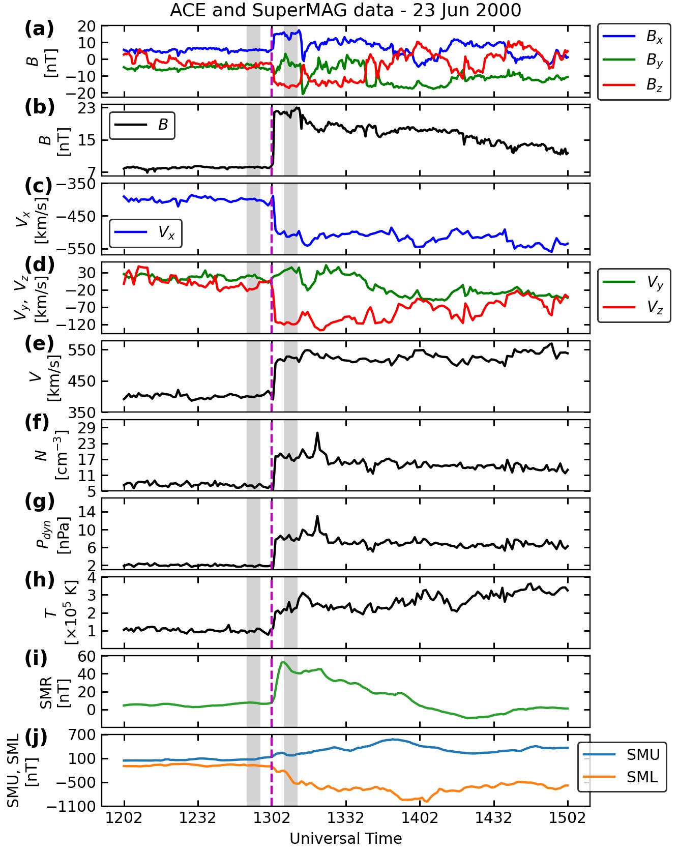
Figure 1, first published by Oliveira and Raeder (2015), shows an IP shock event that occurred on 23 June 2000 observed by ACE at 1226 UT upstream of the Earth at (x, y, z) = (239.9, 36.7, –0.7) , where is the Earth’s radius = 6371.1 km. Solar wind plasma and IMF data are depicted in the figure, along with SuperMAG geomagnetic index data. From top to bottom, the plot shows three components of the IMF (a); IMF magnitude (b); x component of solar wind velocity (c), y and z components of solar wind velocity (d); solar wind velocity magnitude (e); solar wind particle number density (f); solar wind dynamic pressure (g); solar wind thermal temperature (h); SMR index (i); and SMU/SML indices (j). The vertical dashed magenta lines indicate the time of shock impact on the magnetosphere. The data were shifted to the magnetopause nose to match shock observations with the onsets in the ground geomagnetic indices. The highlighted grey areas correspond to the shock upstream region (left) 10 to 5 minutes before shock impact, and shock downstream region (right), 5 to 10 minutes after shock impact. Average values of these regions are used in equations (1-5) for the computation of the shock normal orientations with the five different methods. Most shocks have the time windows mentioned above, but a few events have different time windows.
As discussed by Balogh et al. (1995) and Trotta et al. (2022), the length of the upstream and downstream windows around the shocks is an important factor in determining shock parameters. For example, Trotta et al. (2022) suggested a method to use windows with different lengths with short-length windows being located near the shock. This methodology provides statistical significance (including uncertainties) to the calculated shock parameters and reliability to the subsequent results. This approach will be applied to this shock list in a future work for further improvements of this shock data base.
The data shown in the figure is processed before plotting and before computing shock parameters and normal orientations. First, bad data points, such as 1E+31 are replaced by nan (“not a number”) values and subsequently linearly interpolated. Then, solar wind parameter data are interpolated, and IMF data are averaged to a uniform time cadence of 30 seconds. Differences between the non-interpolated and interpolated data are very small or nearly nonexistent around the shock onset. This process allows the time resolutions of both data sets to match to further perform computations that involve both data sets. The same technique was applied to all events in the shock data base.
Positive step-like enhancements are seen in all solar wind plasma parameters and IMF. This is a clear signature of a fast forward IP shock (Priest, 1981; Tsurutani et al., 2011; Oliveira, 2017). More information on the analysis of this event including shock normal orientations will be provided in the next section.
4 The IP shock data base
Previous versions of this current shock data base were published by Oliveira and Raeder (2015) and Oliveira et al. (2018). A few sources were used to compile these previous shock lists: a shock catalog provided by the Harvard-Smithsonian Center for Astrophysics and compiled by Dr. J. C. Kasper for Wind (http://www.cfa.harvard.edu/shocks/wi_data/) and ACE (http://www.cfa.harvard.edu/shocks/ac_master_data/); a shock list compiled by the ACE team (athttp://www-ssg.sr.unh.edu/mag/ace/ACElists/obs_list.html#shocks.); and another list published by Wang et al. (2010) with events from February 1998 to August 2008. New events were added by scanning solar wind and IMF data to detect shock events that satisfy the framework discussed in section 2.3.
The IP shock data base consists of three files: (i) full_shock_list_2023.txt, a text file with 603 events; (ii) full_shock_params.cdf, a cdf file with detailed information about each specific shock event; and (iii) read_shock.py, a file that contains a short python routine to read information about a specific shock event. The SpacePy package (https://spacepy.github.io, Morley et al., 2011; Larsen et al., 2022) is required to extract shock information from the cdf file using read_shock.py.
The Python routine to read the information of a specific shock event is
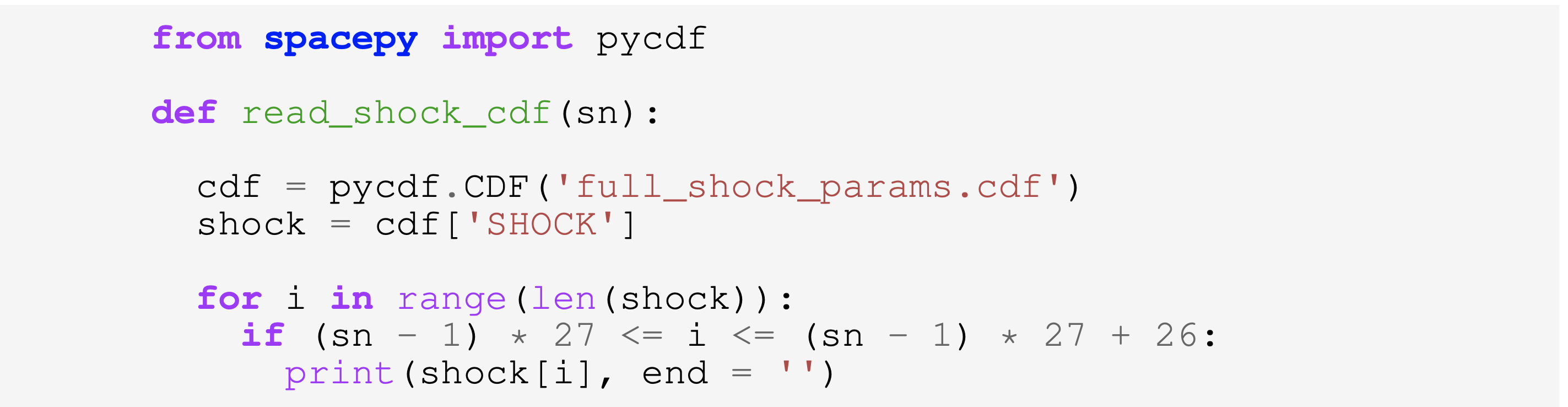
The input variable for the above routine is the shock number sn. The IP shock represented in Figure 1 is the event number 142 in the shock list. Therefore, read_shock.py can be run as follows
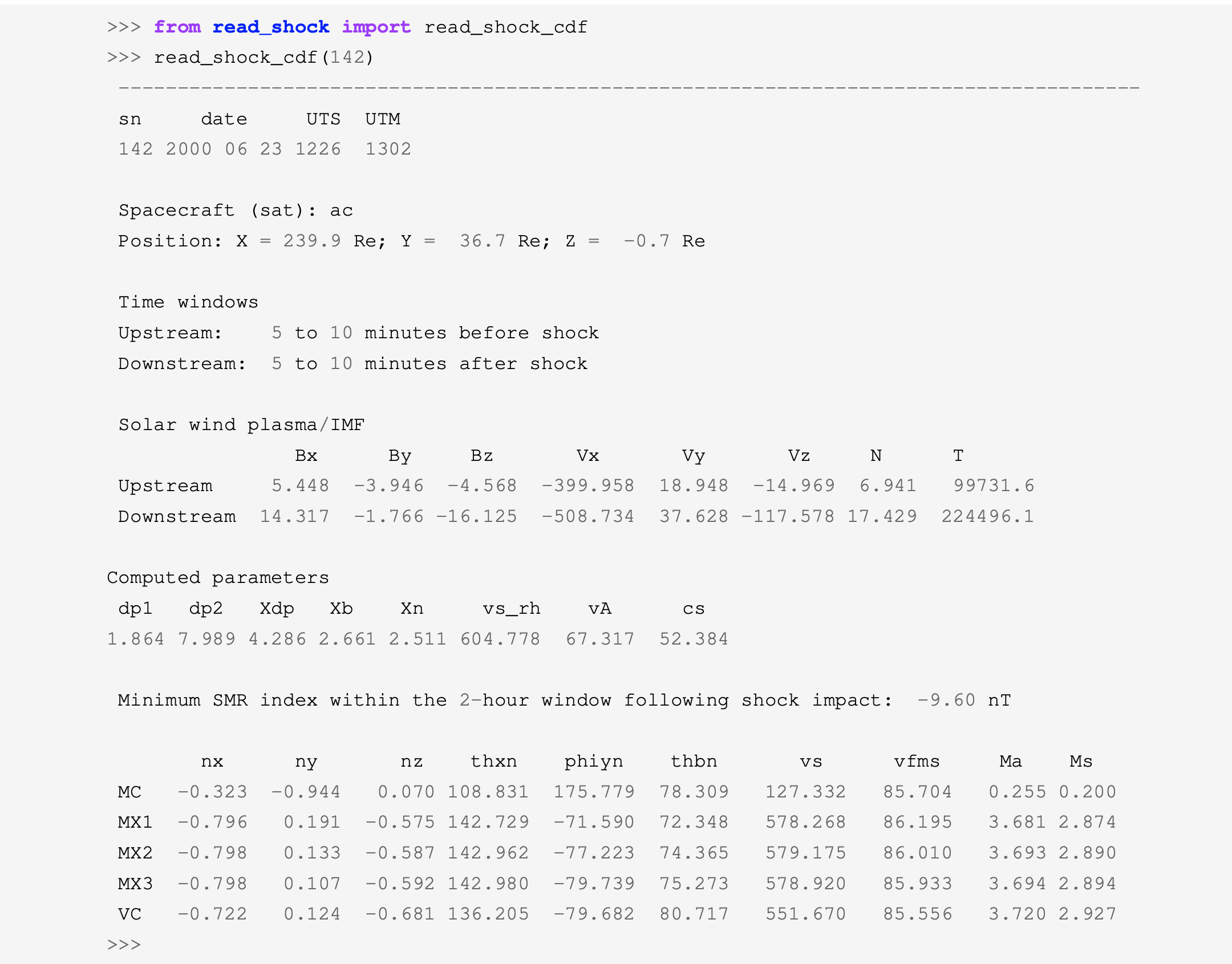
The results for each shock are used to compose the shock list in the full_shock_list_2023.txt file. The file brings a header with the names of the variables (Table 1). The list also includes the position (in ) of the solar wind monitor (either Wind or ACE) whose data are used in the calculations, along with minimum SMR values occurring in a time window of two hours after shock impact. This time window was chosen because amplitudes of geomagnetic activity response usually occur 60 minutes after energy being released by the magnetotail (Bargatze et al., 1985; Oliveira and Raeder, 2015; Oliveira et al., 2021). Such values can be used in studies that aim to use shock observations during non-storm times.
| 1 | sn | shock number; | |
|---|---|---|---|
| 2 | YY | year; | |
| 3 | MM | month; | |
| 4 | DD | day; | |
| 5 | UTS | UT of shock observation by solar wind monitor; | |
| 6 | UTM | UT of ground magnetic sudden impulse onset; | |
| 7 | nx | x component of shock normal vector; | |
| 8 | ny | y component of shock normal vector; | |
| 9 | nz | z component of shock normal vector; | |
| 10 | thxn | shock impact angle (degrees); | |
| 11 | phiyn | shock clock angle in the yz plane (degrees); | |
| 12 | thbn | shock obliquity angle (degrees); | |
| 13 | vs | shock speed (km/s); | |
| 14 | cs | sound speed (km/s); | |
| 15 | vA | Alfvén speed (km/s); | |
| 16 | vfms | fast magnetosonic speed (km/s); | |
| 17 | Ma | Alfvénic Mach number; | |
| 18 | Ms | magnetosonic Mach number; | |
| 19 | dp1 | upstream solar wind dynamic pressure (nPa); | |
| 20 | dp2 | downstream solar wind dynamic pressure (nPa); | |
| 21 | Xn | solar wind number density compression ratio; | |
| 22 | Xdp | solar wind dynamic pressure ratio (dp2/dp1); | |
| 23 | Xb | magnetic field compression ratio; | |
| 24 | bz1 | upstream z component of interplanetary magnetic field (nT); | |
| 25 | bz2 | downstream z component of interplanetary magnetic field (nT); | |
| 26 | sat | satellite used for calculations: 1 for Wind, 2 for ACE | |
| 27 | x | x GSE position (in Re) of solar wind monitor at UTS; | |
| 28 | y | y GSE position (in Re) of solar wind monitor at UTS; | |
| 29 | z | z GSE position (in Re) of solar wind monitor at UTS; | |
| 30 | minSMR | minimum SMR within two hours of shock impact |
Below are the steps taken to include a specific solution for each shock in the full_shock_list_2023.txt list. These are the major revisions made to the list in comparison to its previous versions:
-
1.
A filter is passed on the data to replace bad data points (e.g., 1E+31) by nan values which are then replaced by interpolated/averaged values to a common time cadence for both data sets (IMF and solar wind parameter data).
-
2.
The satellite (Wind or ACE) must be in the solar wind upstream of the Earth (x 14 ).
-
3.
If data of both satellites are simultaneously available, the data set with data of superior quality is used for computations.
-
4.
Events with either or (or both) smaller than one are generally discarded. Events with such conditions are only included in the list if they trigger significant geomagnetic activity, such as SMR variations of at least 15 nT.
-
5.
The solution obtained from equations (1-5) closest to the median value is selected to be included in the list. If the difference between the maximum and minimum values of is larger than 30∘, the solution chosen for the list will be the one that shows more agreement with ground geomagnetic response, represented by the SuperMAG indices (SMR, SMU, SML, SME), as shown in previous publications (e.g., Wang et al., 2006; Oliveira and Raeder, 2015; Rudd et al., 2019; Oliveira et al., 2021).
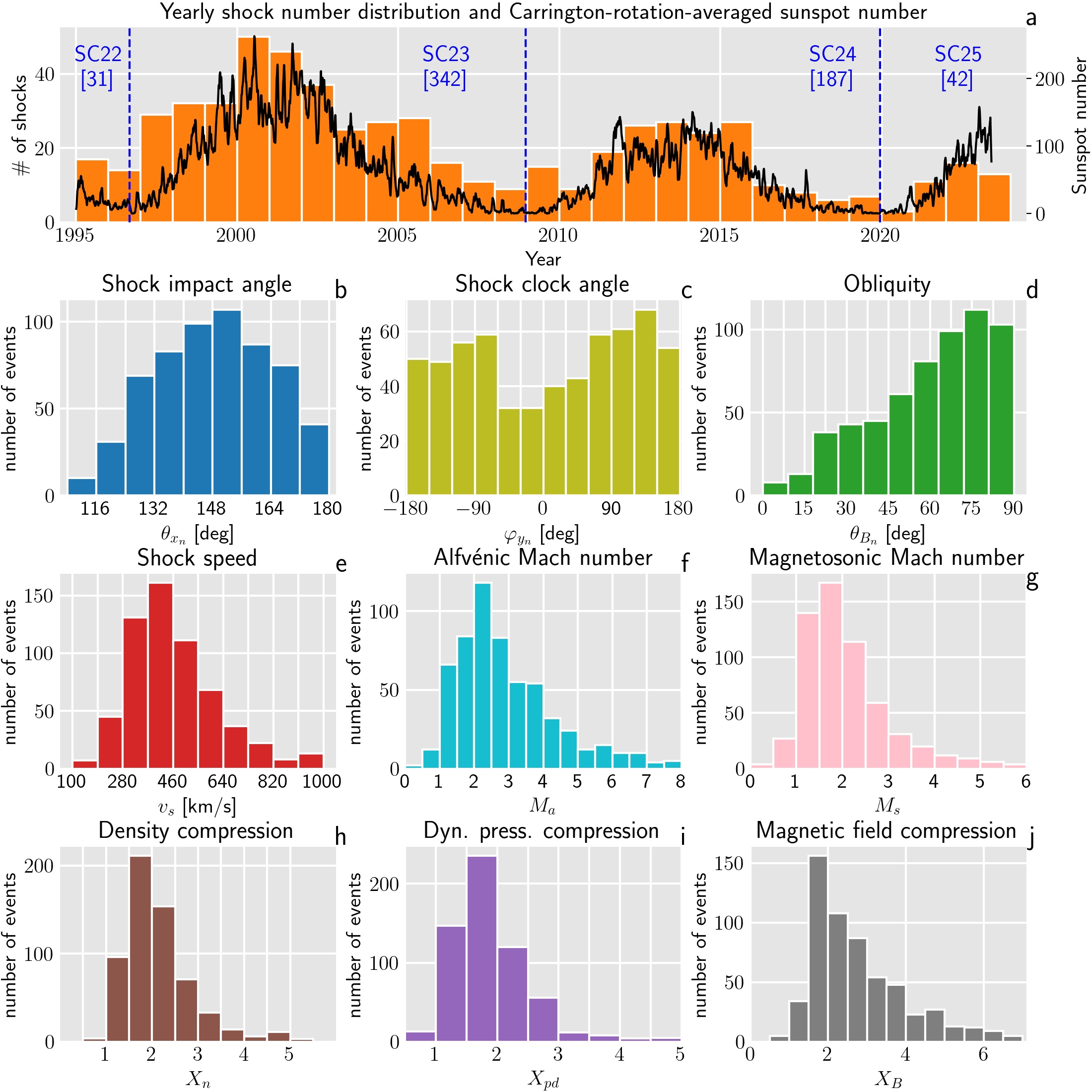
The list version published by Oliveira and Raeder (2015) had 461 events, whereas the list published by Oliveira et al. (2018) had 547 events. This current data base has more events (603) and has a number of additional solar wind parameters and shock properties, which are shown in Table 1. The list time span, January 1995 to May 2023, includes two entire solar cycles (SC23 and SC24), the end of declining phase of SC22, and the beginning of ascending phase of SC25. Therefore, this data base provides a solid number of events for future statistical studies given an appropriate availability of data sets to be investigated.
Figure 2 represents general statistical features of the 603 events in the shock data base. Panel a shows yearly shock number distributions and Carrington-rotation of 25.38 days (Carrington, 1863) averaged sunspot numbers (solid black line). This figure shows a clear correlation between the number of events and sunspot numbers, a result that is already well known (Kilpua et al., 2015; Oliveira and Raeder, 2015; Rudd et al., 2019). Observations show that SC23 was significantly stronger than SC24 based on the overall sunspot numbers, which is reflected on the total number of shocks observed in the corresponding periods (432 and 187, respectively). Zhu et al. (2022) predicted that SC25 will be stronger than SC24 and will reach its maximum value around July 2025. Therefore, according to these predictions, it is reasonable to expect that SC25 will have a similar number of shocks with respect to SC24.
The overall statistical properties of sunspot observations and shock parameters are quantified and shown in Table 2. These results, including mean, median, percentile values, and shock number distribution correlation with sunspot numbers, are in excellent agreement with past studies (Oliveira and Raeder, 2015; Kilpua et al., 2015; Oliveira et al., 2018; Rudd et al., 2019).
| Shock parameters | ||||||
| variable | LPT | median | mean | UPT | STD | of events |
| [∘] | 132.96 | 148.43 | 147.99 | 163.56 | 15.90 | 603 |
| [∘] | -105.87 | 13.10 | 7.12 | 120.00 | 108.41 | 603 |
| [∘] | 41.05 | 64.14 | 59.87 | 79.77 | 21.16 | 603 |
| [km/s] | 335.83 | 435.68 | 463.20 | 575.75 | 161.88 | 603 |
| 1.74 | 2.58 | 3.13 | 4.05 | 1.95 | 603 | |
| 1.33 | 1.86 | 2.16 | 2.79 | 1.18 | 603 | |
| 1.54 | 1.96 | 2.13 | 2.62 | 0.75 | 603 | |
| 1.45 | 1.79 | 1.93 | 2.36 | 0.69 | 603 | |
| 1.81 | 2.49 | 2.98 | 3.86 | 1.56 | 603 | |
| Sunspot numbers (complete solar cycles) | ||||||
| solar cyle | LPT | median | mean | UPT | STD | of events |
| SC23 | 13.00 | 63.00 | 82.39 | 150.00 | 72.74 | 342 |
| SC24 | 11.00 | 44.00 | 54.08 | 98.00 | 47.01 | 187 |
5 Suggested use of the IP shock data base
The IP shock data base described in this report can be used in many ways. For example, this list can be used in studies involving geomagnetic activity following shock impacts from the geospace to the ground, including particle acceleration by shocks, particle dynamics and energization in the radiation belts, magnetospheric ultra-low frequency (ULF) waves, magnetic field response in geosynchronous orbit, field-aligned currents, role of shocks in substorm triggering, ionospheric irregularities, high-latitude thermosphere response (neutral density and nitric oxide) to shock impacts, ground magnetometer response (dB/dt variations) and subsequent effects on GICs, and many others. Therefore, this shock list can be used in a variety of space physics and space weather investigations.
A major feature of this shock list is the possibility of using the shock impact angle as a factor controlling geomagnetic activity. Oliveira (2023) has recently reviewed the effects of shock impact angles on the subsequent geomagnetic activity and also suggested a few topics for future research.
- 1.
- 2.
- 3.
- 4.
- 5.
Finally, I would like to urge researchers to perform numerical simulations of shocks with different orientations. For example, Welling et al. (2021) argued that the “most perfect” CME would be very fast and impact Earth head-on. They performed numerical simulations of the impact of a perfect CME on the magnetosphere and concluded that ground d/d variations were noted in very low latitude regions because the CME impact was purely frontal. Furthermore, our shock list can be very useful in simulations comparing real observations with results yielded by numerical simulations of shocks with different orientations for many different space weather purposes.
Data Availability Statement
The IP shock data base can be downloaded from Zenodo (https://zenodo.org/record/7991430). The solar wind plasma and IMF data observed by Wind and ACE used to calculate the shock impact angles including shock properties were obtained from the CDAWeb (Coordinated Data Analysis) website provided by NASA Goddard Space Flight Center’s Space Physics Data Facility (http://cdaweb.gsfc.nasa.gov). The geomagnetic index data used in this publication were downloaded from the SuperMAG initiative website: https://supermag.jhuapl.edu. Sunspot number data was downloaded from the SILSO (Sunspot Index and Long-term Solar Observations) website (https://www.sidc.be/silso/datafiles).
Conflict of Interest Statement
The author declares that the research was conducted in the absence of any commercial or financial relationships that could be construed as a potential conflict of interest.
Author Contributions
This data report article was written by the author without any direct contributions from others.
Funding
This work was possible thanks to the financial support provided by the NASA HGIO program through grant 80NSSC22K0756.
References
- Abda et al. (2020) Abda, Z. M. K., Aziz, N. F. A., Kadir, M. Z. A. A., and Rhazali, Z. A. (2020). A Review of Geomagnetically Induced Current Effects on Electrical Power System: Principles and Theory. IEEE Access 8, 200237–200258. 10.1109/ACCESS.2020.3034347
- Abraham-Shrauner (1972) Abraham-Shrauner, B. (1972). Determination of magnetohydronamic shock normals. Journal of Geophysical Research 77, 736–739. 10.1029/JA077i004p00736
- Aguilar-Rodriguez et al. (2010) Aguilar-Rodriguez, E., Blanco-Cano, X., Russell, C. T., Jian, L. K., Luhmann, J. G., and Velez, J. C. R. (2010). Study of interplanetary shocks using multi‐spacecraft observations. In Twelth International Solar Wind Conference, AIP Conference Proceedings, eds. M. Maksimovic, K. Issautier, N. Meyer‐Vernet, M. Moncuquet, and F. Pantellini (Washington, D.C.: American Institute of Physics), vol. 1216, 467–470. 10.1063/1.3395904
- Baker (2019) Baker, A. B. (2019). Effect of Interplanetary Shock Impact Angle on the Occurrence Rate and Properties of Pc5 Waves Observed by High-Latitude Ground Magnetometers. Master’s thesis, Virginia Tech, Blacksburg, Virginia
- Balogh et al. (1995) Balogh, A., Gonzalez-Esparza, J. A., Forsyth, R. J., Burton, M. E., Goldstein, B. E., Smith, E. J., et al. (1995). Interplanetary shock waves: Ulysses observations in and out of the ecliptic plane. Space Science Reviews , 171–18010.1007/BF00768774
- Bargatze et al. (1985) Bargatze, L. F., Baker, D. N., McPherron, R. L., and Jr., E. W. H. (1985). Magnetospheric impulse response for many levels of geomagnetic activity. Journal of Geophysical Research 90, 6387–6394. 10.1029/JA090iA07p06387
- Bhaskar et al. (2021) Bhaskar, A., Sibeck, D., Kanekal, S. G., Singer, H. J., Reeves, G., Oliveira, D. M., et al. (2021). Radiation belt response to fast reverse shock at geosynchronous orbit. The Astrophysical Journal 910, 154. 10.3847/1538-4357/abd702
- Boyd and Sanderson (2003) Boyd, T. J. M. and Sanderson, J. J. (2003). The Physics of Plasmas (Cambridge, United Kingdom: Cambridge University Press)
- Burlaga (1971) Burlaga, L. F. (1971). Hydromagnetic waves and discontinuities in the solar wind. Space Science Reviews 12, 600–657. 10.1007/BF00173345
- Cameron et al. (2019) Cameron, T. G., Jackel, B. J., and Oliveira, D. M. (2019). Using mutual information to investigate geoeffectiveness of solar wind phase fronts with different front orientations. Journal of Geophysical Research: Space Physics 124, 1582–1592. 10.1029/2018JA026080
- Carrington (1863) Carrington, R. C. (1863). Observations of the Spots on the Sun, from November 9th 1853 to March 24th 1861 made at Redhill (London, United Kingdom: Williams and Norgate)
- Carter et al. (2015) Carter, B. A., Yizengaw, E., Pradipta, R., Halford, A. J., Norman, R., and Zhang, K. (2015). Interplanetary shocks and the resulting geomagnetically induced currents at the equator. Geophysical Research Letters 42, 6554–6559. 10.1002/2015GL065060
- Clette and Lefèvre (2016) Clette, F. and Lefèvre, L. (2016). The New Sunspot Number: Assembling All Corrections. Solar Physics 291, 2629–2651. 10.1007/s11207-016-1014-y
- Colburn and Sonett (1966) Colburn, D. S. and Sonett, C. P. (1966). Discontinuities in the solar wind. Space Science Reviews 5, 439–506. 10.1007/BF00240575
- Craven et al. (1986) Craven, J. D., Frank, L. A., Russell, C. T., Smith, E. E., and Lepping, R. P. (1986). Global auroral responses to magnetospheric compressions by shocks in the solar wind: Two case studies. In Solar Wind-Magnetosphere Coupling, eds. Y. Kamide and J. A. Slavin (Tokyo, Japan: Terra Scientific), 367–380
- Davis and Sugiura (1966) Davis, T. N. and Sugiura, M. (1966). Auroral electrojet activity index AE and its universal time variations. Journal of Geophysical Research 71, 785–801. 10.1029/JZ071i003p00785
- Echer et al. (2023) Echer, E., de Lucas, A., Hajra, R., de Souza Franco, A. M., Bolzan, M. J. A., and do Nascimento, L. E. S. (2023). Geomagnetic Activity Following Interplanetary Shocks in Solar Cycles 23 and 24. Brazilian Journal of Physics 53, 1–13. 10.1007/s13538-023-01294-w
- Echer et al. (2005) Echer, E., Gonzalez, W. D., Guarnieri, F. L., Dal Lago, A., and Vieira, L. E. A. (2005). Introduction to space weather. Advances in Space Research 35, 855–865. 10.1016/j.asr.2005.02.098
- Gjerloev (2009) Gjerloev, J. W. (2009). A global ground-based magnetometer initiative. Eos Transactions AGU 90, 230–231. 10.1029/2009EO270002
- Goncharov et al. (2014) Goncharov, O., S̆afránková, J., N̆emec̆ek, Z., Pr̆ech, L., Pitn̆a, A., and Zastenker, G. N. (2014). Upstream and downstream wave packets associated with low-Mach number interplanetary shocks. Geophysical Research Letters 41, 8100–8106. 10.1002/2014GL062149
- Guo et al. (2005) Guo, X.-C., Hu, Y.-Q., and Wang, C. (2005). Earth’s magnetosphere impinged by interplanetary shocks of different orientations. Chinese Physics Letters 22, 3221–3224. 10.1088/0256-307X/22/12/067
- Hajra and Tsurutani (2018a) Hajra, R. and Tsurutani, B. T. (2018a). Interplanetary Shocks Inducing Magnetospheric Supersubstorms (SML 2500 nT): Unusual Auroral Morphologies and Energy Flow. The Astrophysical Journal 858. 10.3847/1538-4357/aabaed
- Hajra and Tsurutani (2018b) Hajra, R. and Tsurutani, B. T. (2018b). Magnetospheric “Killer” Relativistic Electron Dropouts (REDs) and Repopulation: A Cyclical Process. In Extreme Events in Geospace: Origins, Predictability and Consequences, ed. N. Buzulukova (Cambridge, MA: Elsevier), 373–400. 10.1016/B978-0-12-812700-1.00014-5
- Hartinger et al. (2022) Hartinger, M. D., Takahashi, K., Drozdov, A. Y., Shi, X., Usanova, M. E., and Kress, B. (2022). ULF Wave Modeling, Effects, and Applications: Accomplishments, Recent Advances, and Future. Frontiers in Astronomy and Space Science 9. 10.3389/fspas.2022.867394
- Jeffrey and Taniuti (1964) Jeffrey, A. and Taniuti, T. (1964). Nonlinear Wave Propagation (New York, NY: Academic Press)
- Kabin (2001) Kabin, K. (2001). A note on the compression ratio in MHD shocks. Journal of Plasma Physics 66, 259–274. 10.1017/S0022377801001295
- Khazanov (2016) Khazanov, G. V. (2016). Space Weather Fundamentals (Boca Raton, FL: CRC Press)
- Kilpua et al. (2015) Kilpua, E. K. J., Lumme, K., E. Andréeová, Isavnin, A., and Koskinen, H. E. J. (2015). Properties and drivers of fast interplanetary shocks near the orbit of the Earth (1995-2013). Journal of Geophysical Research: Space Physics 120, 4112–4125. 10.1002/2015JA021138
- Larsen et al. (2022) Larsen, B. A., Morley, S. K., Niehof, J. T., and Welling, D. T. (2022). SpacePy. 10.5281/zenodo.3252523
- Lepping et al. (1995) Lepping, R. P., Acuña, M. H., Burlaga, L. F., Farrell, W. M., Slavin, J. A., Schatten, K. H., et al. (1995). The WIND Magnetic Field Investigation. Space Science Reviews 71, 207–229. 10.1007/BF00751330
- McComas et al. (1998) McComas, D. J., Bame, S. J., Barker, P., Feldman, W. C., Phillips, J. L., Riley, P., et al. (1998). Solar Wind Electron Proton Alpha Monitor (SWEPAM) for the Advanced Composition Explorer. Space Science Reviews 86, 563–612. 10.1023/A:1005040232597
- Morley et al. (2011) Morley, S. K., Koller, J., Welling, D. T., Larsen, B. A., Henderson, M. G., and Niehof, J. T. (2011). Spacepy - A Python-based library of tools for the space sciences. In Proceedings of the 9th Python in science Conference (SciPy 2010) (Austin, TX), 67–72
- Newell and Gjerloev (2011) Newell, P. T. and Gjerloev, J. W. (2011). Evaluation of SuperMAG auroral electrojet indices as indicators of substorms and auroral power. Journal of Geophysical Research 116. 10.1029/2011JA016779
- Newell and Gjerloev (2012) Newell, P. T. and Gjerloev, J. W. (2012). SuperMAG-based partial ring current indices. Journal of Geophysical Research 117, 1–15. 10.1029/2012JA017586
- Ogilvie et al. (1995) Ogilvie, K. W., Chornay, D. J., Fritzenreiter, R. J., Hunsaker, F., Keller, J., Lobell, J., et al. (1995). SWE, a comprehensive plasma instrument for the WIND spacecraft. Space Science Reviews 71, 55–77. 10.1007/BF00751326
- Oh et al. (2007) Oh, S. Y., Yi, Y., and Kim, Y. H. (2007). Solar cycle variation of the interplanetary forward shock drivers observed at 1 AU. Solar Physics 245, 391–410. 10.1007/s11207-007-9042-2
- Oliveira (2017) Oliveira, D. M. (2017). Magnetohydrodynamic shocks in the interplanetary space: A theoretical review. Brazilian Journal of Physics 47, 81–95. 10.1007/s13538-016-0472-x
- Oliveira (2023) Oliveira, D. M. (2023). Geoeffectiveness of Interplanetary Shocks Controlled by Impact Angles: Past Research, Recent Advancements, and Future Work. Frontiers in Astronomy and Space Science 10. 10.3389/fspas.2023.1179279
- Oliveira et al. (2018) Oliveira, D. M., Arel, D., Raeder, J., Zesta, E., Ngwira, C. M., Carter, B. A., et al. (2018). Geomagnetically induced currents caused by interplanetary shocks with different impact angles and speeds. Space Weather 16, 636–647. 10.1029/2018SW001880
- Oliveira et al. (2020) Oliveira, D. M., Hartinger, M. D., Xu, Z., Zesta, E., Pilipenko, V. A., Giles, B. L., et al. (2020). Interplanetary shock impact angles control magnetospheric ULF wave activity: Wave amplitude, frequency, and power spectra. Geophysical Research Letters 47, e2020GL090857. 10.1029/2020GL090857
- Oliveira and Ngwira (2017) Oliveira, D. M. and Ngwira, C. M. (2017). Geomagnetically Induced Currents: Principles. Brazilian Journal of Physics 47, 552–560. 10.1007/s13538-017-0523-y
- Oliveira and Raeder (2014) Oliveira, D. M. and Raeder, J. (2014). Impact angle control of interplanetary shock geoeffectiveness. Journal of Geophysical Research: Space Physics 119, 8188–8201. 10.1002/2014JA020275
- Oliveira and Raeder (2015) Oliveira, D. M. and Raeder, J. (2015). Impact angle control of interplanetary shock geoeffectiveness: A statistical study. Journal of Geophysical Research: Space Physics 120, 4313–4323. 10.1002/2015JA021147
- Oliveira et al. (2016) Oliveira, D. M., Raeder, J., Tsurutani, B. T., and Gjerloev, J. W. (2016). Effects of interplanetary shock inclinations on nightside auroral power intensity. Brazilian Journal of Physics 46, 97–104. 10.1007/s13538-015-0389-9
- Oliveira and Samsonov (2018) Oliveira, D. M. and Samsonov, A. A. (2018). Geoeffectiveness of interplanetary shocks controlled by impact angles: A review. Advances in Space Research 61, 1–44. 10.1016/j.asr.2017.10.006
- Oliveira et al. (2021) Oliveira, D. M., Weygand, J. M., Zesta, E., Ngwira, C. M., Hartinger, M. D., Xu, Z., et al. (2021). Impact angle control of local intense d/d variations during shock-induced substorms. Space Weather 19, e2021SW002933. 10.1029/2021SW002933
- Oliveira and Zesta (2019) Oliveira, D. M. and Zesta, E. (2019). Satellite Orbital Drag During Magnetic Storms. Space Weather 17, 1510–1533. 10.1029/2019SW002287
- Pizzo (1991) Pizzo, V. J. (1991). The evolution of corotating stream fronts near the ecliptic plane in the inner solar system: 2. Three-dimensional tilted-dipole fronts. Journal of Geophysical Research 96, 5405–5420. 10.1029/91JA00155
- Priest (1981) Priest, E. F. (1981). Solar Magnetohydrodynamics (Dordrecht, Holland: D. Reidel Publishing)
- Rostoker (1972) Rostoker, G. (1972). Geomagnetic indices. Reviews of Geophysics 10, 935–950. 10.1029/RG010i004p00935
- Rudd et al. (2019) Rudd, J. T., Oliveira, D. M., Bhaskar, A., and Halford, A. J. (2019). How do interplanetary shock impact angles control the size of the geoeffective magnetosphere? Advances in Space Research 63, 317–326. 10.1016/j.asr.2018.09.013
- Russell (2000) Russell, C. (2000). The solar wind interaction with the Earth’s magnetosphere: A tutorial. IEEE Trans. Plasma Sci. 28, 1818–1830. 10.1109/27.902211
- Russell et al. (1983) Russell, C. T., Gosling, J. T., Zwickl, R. D., and Smith, E. J. (1983). Multiple spacecraft observations of interplanetary shocks: ISEE three-dimensional plasma measurements. Journal of Geophysical Research 88, 9941–9947. 10.1029/JA088iA12p09941
- Samsonov et al. (2015) Samsonov, A. A., Sergeev, V. A., Kuznetsova, M. M., and Sibeck, D. G. (2015). Asymmetric magnetospheric compressions and expansions in response to impact of inclined interplanetary shock. Geophysical Research Letters 42, 4716–4722. 10.1002/2015GL064294
- Schwartz (1998) Schwartz, S. J. (1998). Shock and discontinuity normals, Mach numbers, and related parameters. In Analysis Methods for Multi-Spacecraft Data, eds. G. Paschmann and P. W. Daly (Noordwijk, The Netherlands: ESA Publications Division), no. SR-001 in ISSI Scientific Report, 249–270
- Selvakumaran et al. (2017) Selvakumaran, R., Veenadhari, B., Ebihara, Y., Kumar, S., and Prasad, D. S. V. V. D. (2017). The role of interplanetary shock orientation on SC/SI rise time and geoeffectiveness. Advances in Space Research 59, 1425–1434. 10.1016/j.asr.2016.12.010
- Shi et al. (2019) Shi, Y., Oliveira, D. M., Knipp, D. J., Zesta, E., Matsuo, T., and Anderson, B. (2019). Effects of Nearly Frontal and Highly Inclined Interplanetary Shocks on High-latitude Field-aligned Currents (FACs). Space Weather 17, 1659–1673. 10.1029/2019SW002367
- Smith et al. (2020) Smith, A. W., Rae, J., Forsyth, C., Oliveira, D. M., Freeman, P. M., and Jackson, D. (2020). Probabilistic Forecasts of Storm Sudden Commencements from Interplanetary Shocks using Machine Learning. Space Weather 18, e2020SW002603. 10.1029/2020SW002603
- Smith et al. (1998) Smith, C. W., L’Heureux, J., Ness, N. F., Acuña, M. H., Burlaga, L. F., and Scheifele, J. (1998). The ACE magnetic fields experiment. Space Science Reviews 86, 613–632. 10.1023/A:1005092216668
- Stone and Tsurutani (1985) Stone, R. G. and Tsurutani, B. T. (eds.) (1985). Collisionless Shocks in the Heliosphere: A Tutorial Review, Geophysical Monograph Series, vol. 34 (Washington, D.C.: American Geophysical Union). 10.1029/GM034
- Takeuchi et al. (2002) Takeuchi, T., Russell, C. T., and Araki, T. (2002). Effect of the orientation of interplanetary shock on the geomagnetic sudden commencement. Journal of Geophysical Research 107, SMP 6–1–SMP 6–10. 10.1029/2002JA009597
- Trotta et al. (2023) Trotta, D., Hietala, H., Horbury, T., Dresing, N., Vainio, R., Wilson III, L., et al. (2023). Multi-spacecraft observations of shocklets at an interplanetary shock. Monthly Notices of the Royal Astronomical Society 520. 10.1093/mnras/stad104
- Trotta et al. (2022) Trotta, D., Vuorinen, L., Hietala, H., Horbury, T., Dresing, N., Gieseler, J., et al. (2022). Single-spacecraft techniques for shock parameters estimation: A systematic approach. Frontiers in Astronomy and Space Science 9. 10.3389/fspas.2022.1005672
- Tsurutani et al. (2006) Tsurutani, B. T., Gonzalez, W. D., Gonzalez, A. L. C., Guarnieri, F. L., Gopalswamy, N., Grande, M., et al. (2006). Corotating solar wind streams and recurrent geomagnetic activity: A review. Journal of Geophysical Research 111, 1–25. 10.1029/2005JA011273
- Tsurutani and Hajra (2023) Tsurutani, B. T. and Hajra, R. (2023). Energetics of Shock-triggered Supersubstorms (SML –2500 nT). The Astrophysical Journal 946. 10.3847/1538-4357/acb143
- Tsurutani et al. (2016) Tsurutani, B. T., Hajra, R., Tanimori, T., Takada, A., Remya, B., Mannucci, A. J., et al. (2016). Heliospheric plasma sheet (HPS) impingement onto the magnetosphere as a cause of relativistic electron dropouts (REDs) via coherent EMIC wave scattering with possible consequences for climate change mechanisms. Journal of Geophysical Research: Space Physics 121, 10,130–10,156. 10.1002/2016JA022499
- Tsurutani et al. (2011) Tsurutani, B. T., Lakhina, G. S., Verkhoglyadova, O. P., Gonzalez, W. D., Echer, E., and Guarnieri, F. L. (2011). A review of interplanetary discontinuities and their geomagnetic effects. Journal of Atmospheric and Solar-Terrestrial Physics 73, 5–19. 10.1016/j.jastp.2010.04.001
- Wang et al. (2006) Wang, C., Li, C. X., Huang, Z. H., and Richardson, J. D. (2006). Effect of interplanetary shock strengths and orientations on storm sudden commencement rise times. Geophysical Research Letters 33, 1–3. 10.1029/2006GL025966
- Wang et al. (2010) Wang, C., Li, H., Richardson, J. D., and Kan, J. R. (2010). Interplanetary shock characteristics and associated geosynchronous magnetic field variations estimated from sudden impulses observed on the ground. Journal of Geophysical Research 115. 10.1029/2009JA014833
- Welling et al. (2021) Welling, D. T., Love, J. J., Joshua Rigler, E., Oliveira, D. M., Komar, C. M., and Morley, S. K. (2021). Numerical simulations of the geospace response to a perfect interplanetary coronal mass ejection. Space Weather 19, e2020SW002489. 10.1029/2020SW002489
- Xu et al. (2020) Xu, Z., Hartinger, M. D., Oliveira, D. M., Coyle, S., Clauer, C. R., Weimer, D., et al. (2020). Inter-hemispheric asymmetries in the ground magnetic response to interplanetary shocks: The role of shock impact angle. Space Weather 18, e2019SW002427. 10.1029/2019SW002427
- Zesta and Oliveira (2019) Zesta, E. and Oliveira, D. M. (2019). Thermospheric heating and cooling times during geomagnetic storms, including extreme events. Geophysical Research Letters 46, 12,739–12,746. 10.1029/2019GL085120
- Zhu et al. (2022) Zhu, H., Zhu, W., and He, M. (2022). Solar Cycle 25 Prediction Using an Optimized Long Short-Term Memory Mode with F10.7. Solar Physics 297. 10.1007/s11207-022-02091-5