Random Word Data Augmentation with CLIP for Zero-Shot Anomaly Detection

Abstract

This paper presents a novel method that leverages a visual-language model, CLIP, as a data source for zero-shot anomaly detection. Tremendous efforts have been put towards developing anomaly detectors due to their potential industrial applications. Considering the difficulty in acquiring various anomalous samples for training, most existing methods train models with only normal samples and measure discrepancies from the distribution of normal samples during inference, which requires training a model for each object category. The problem of this inefficient training requirement has been tackled by designing a CLIP-based anomaly detector that applies prompt-guided classification to each part of an image in a sliding window manner. However, the method still suffers from the labor of careful prompt ensembling with known object categories. To overcome the issues above, we propose leveraging CLIP as a data source for training. Our method generates text embeddings with the text encoder in CLIP with typical prompts that include words of normal and anomaly. In addition to these words, we insert several randomly generated words into prompts, which enables the encoder to generate a diverse set of normal and anomalous samples. Using the generated embeddings as training data, a feed-forward neural network learns to extract features of normal and anomaly from CLIP’s embeddings, and as a result, a category-agnostic anomaly detector can be obtained without any training images. Experimental results demonstrate that our method achieves state-of-the-art performance without laborious prompt ensembling in zero-shot setups.

1 Introduction

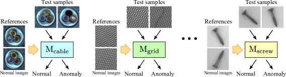
(a) Vanilla AD.

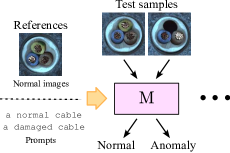
(b) Category-agnostic known-object AD.

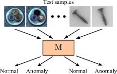
(c) Category-agnostic unknown-object AD (ours).

Figure 1: Existing and our AD methods. (a) Existing vanilla AD methods train a model for each object category with normal samples as references and then test the models with the samples of the target object categories. (b) Existing category-agnostic methods do not require category-specific models. However, target object information such as normal images and prompts must be provided during inference. (c) Our method does not need either category-specific models or target object information during inference.

Visual anomaly detection (AD) is the task of classifying images as normal or anomaly, where anomalous images typically capture damaged, broken, or defective objects. AD differs from object classification in that anomalous samples are defined as those different from normal samples and thus are not restricted to specific categories. Due to the diverse appearances of anomalous samples, AD remains a challenging problem and thus has been tackled by numerous works [Golan and El-Yaniv(2018), Ruff et al.(2018)Ruff, Vandermeulen, Goernitz, Deecke, Siddiqui, Binder, Müller, and Kloft, Gong et al.(2019)Gong, Liu, Le, Saha, Mansour, Venkatesh, and Hengel, Bergmann et al.(2019)Bergmann, Fauser, Sattlegger, and Steger, Ye et al.(2019)Ye, Huang, Cao, Li, Zhang, and Lu, Yi and Yoon(2021), Cohen and Hoshen(2020), Bergmann et al.(2020)Bergmann, Fauser, Sattlegger, and Steger, Salehi et al.(2021)Salehi, Sadjadi, Baselizadeh, Rohban, and Rabiee, Rudolph et al.(2021)Rudolph, Wandt, and Rosenhahn, Defard et al.(2021)Defard, Setkov, Loesch, and Audigier, Zavrtanik et al.(2021)Zavrtanik, Kristan, and Skocaj, Li et al.(2021)Li, Yoon, Sohn, and Pfister, Sheynin et al.(2021)Sheynin, Benaim, and Wolf, Wu et al.(2021)Wu, Chen, Fuh, and Liu, Roth et al.(2022)Roth, Pemula, Zepeda, Schölkopf, Brox, and Gehler, Zou et al.(2022)Zou, Jeong, Pemula, Zhang, and Dabeer, Bergmann et al.(2022)Bergmann, Batzner, Fauser, Sattlegger, and Steger, Huang et al.(2022)Huang, Guan, Jiang, Zhang, Spratlin, and Wang, Ristea et al.(2022)Ristea, Madan, Ionescu, Nasrollahi, Khan, Moeslund, and Shah, Jeong et al.(2023)Jeong, Zou, Kim, Zhang, Ravichandran, and Dabeer] for real-world applications.

Considering the fact that a diverse set of anomalous samples is difficult to be obtained, most existing methods [Bergmann et al.(2020)Bergmann, Fauser, Sattlegger, and Steger, Bergmann et al.(2022)Bergmann, Batzner, Fauser, Sattlegger, and Steger, Golan and El-Yaniv(2018), Gong et al.(2019)Gong, Liu, Le, Saha, Mansour, Venkatesh, and Hengel, Li et al.(2021)Li, Yoon, Sohn, and Pfister, Ristea et al.(2022)Ristea, Madan, Ionescu, Nasrollahi, Khan, Moeslund, and Shah, Rudolph et al.(2021)Rudolph, Wandt, and Rosenhahn, Ruff et al.(2018)Ruff, Vandermeulen, Goernitz, Deecke, Siddiqui, Binder, Müller, and Kloft, Salehi et al.(2021)Salehi, Sadjadi, Baselizadeh, Rohban, and Rabiee, Sheynin et al.(2021)Sheynin, Benaim, and Wolf, Wu et al.(2021)Wu, Chen, Fuh, and Liu, Ye et al.(2019)Ye, Huang, Cao, Li, Zhang, and Lu, Yi and Yoon(2021), Zavrtanik et al.(2021)Zavrtanik, Kristan, and Skocaj, Zou et al.(2022)Zou, Jeong, Pemula, Zhang, and Dabeer] train models with normal samples and then test on both normal and anomalous samples. The distribution of normal samples is modeled via various methods such as one-class classification [Ruff et al.(2018)Ruff, Vandermeulen, Goernitz, Deecke, Siddiqui, Binder, Müller, and Kloft, Yi and Yoon(2021)], reconstruction [Gong et al.(2019)Gong, Liu, Le, Saha, Mansour, Venkatesh, and Hengel, Wu et al.(2021)Wu, Chen, Fuh, and Liu], and imitation of anomalous samples [Li et al.(2021)Li, Yoon, Sohn, and Pfister, Zavrtanik et al.(2021)Zavrtanik, Kristan, and Skocaj] during training, and discrepancies from the distribution are calculated to predict anomaly scores during inference. Since the methods are built on the assumption that normal samples are nearly identical, one model can only be applied to the objects of the same category as depicted in Fig. 1. This category-specific model requirement demands a significant number of models when the number of target objects is large, which renders the deployment of the methods impractical.

To overcome the aforementioned issue, category-agnostic methods [Cohen and Hoshen(2020), Defard et al.(2021)Defard, Setkov, Loesch, and Audigier, Huang et al.(2022)Huang, Guan, Jiang, Zhang, Spratlin, and Wang, Jeong et al.(2023)Jeong, Zou, Kim, Zhang, Ravichandran, and Dabeer, Roth et al.(2022)Roth, Pemula, Zepeda, Schölkopf, Brox, and Gehler] have been proposed. These methods leverage large-scale pre-trained models to extract highly generalizable features and utilize them as references to detect anomalous samples as illustrated in Fig. 1. In particular, recently proposed WinCLIP [Jeong et al.(2023)Jeong, Zou, Kim, Zhang, Ravichandran, and Dabeer] demonstrates significant performance improvement over the other category-agnostic methods in a zero-shot AD setup, which extends a highly capable vison-language model, the Contrastive Language-Image Pre-training (CLIP) model [Radford et al.(2021)Radford, Kim, Hallacy, Ramesh, Goh, Agarwal, Sastry, Askell, Mishkin, Clark, Krueger, and Sutskever], to AD and is the most similar to our method.

In this paper, we also concentrate on zero-shot AD with CLIP. However, our method differs from WinCLIP in that we employ CLIP as a data source for training anomaly detectors. We leverage the observation that CLIP’s text encoder generates perturbed output embeddings when input sentences are augmented with random words. By this augmentation, we produce a set of highly diverse embeddings with typical prompts containing words of normal and anomaly. These embeddings are then utilized as training data for a feed-forward neural network (FNN), which extracts normal and anomaly features from the embeddings and classifies them accordingly. Since FNN is trained without any object information, our proposed approach is applicable even when target objects are unknown during inference as shown in Fig. 1. Furthermore, our method does not require any laborious prompt ensembling, which is leveraged in WinCLIP to improve performance.

To summarize, our contributions are three-fold:

• We propose a novel AD method that leverages CLIP as a data source for training an FNN. Since our method does not require any target object information during training or inference, the trained model can be applied to the case where anomalous samples of unknown objects must be detected.

• Our method achieves competitive performance to state-of-the-art methods without any prompt ensembling on two benchmark datasets in challenging zero-shot setups.

• Extensive experiments show the potential use case of the proposed method, where anomalous samples contain objects of ambiguous categories.

2 Related Work

2.1 Anomaly Detection

Most existing AD methods [Bergmann et al.(2020)Bergmann, Fauser, Sattlegger, and Steger, Bergmann et al.(2022)Bergmann, Batzner, Fauser, Sattlegger, and Steger, Golan and El-Yaniv(2018), Gong et al.(2019)Gong, Liu, Le, Saha, Mansour, Venkatesh, and Hengel, Li et al.(2021)Li, Yoon, Sohn, and Pfister, Ristea et al.(2022)Ristea, Madan, Ionescu, Nasrollahi, Khan, Moeslund, and Shah, Rudolph et al.(2021)Rudolph, Wandt, and Rosenhahn, Ruff et al.(2018)Ruff, Vandermeulen, Goernitz, Deecke, Siddiqui, Binder, Müller, and Kloft, Salehi et al.(2021)Salehi, Sadjadi, Baselizadeh, Rohban, and Rabiee, Sheynin et al.(2021)Sheynin, Benaim, and Wolf, Wu et al.(2021)Wu, Chen, Fuh, and Liu, Ye et al.(2019)Ye, Huang, Cao, Li, Zhang, and Lu, Yi and Yoon(2021), Zavrtanik et al.(2021)Zavrtanik, Kristan, and Skocaj, Zou et al.(2022)Zou, Jeong, Pemula, Zhang, and Dabeer] employ category-specific models to capture the distribution of normal samples during training and then calculate the discrepancies from the distribution during inference. One major trend of training category-specific models is to use unsupervised learning. An early attempt [Ruff et al.(2018)Ruff, Vandermeulen, Goernitz, Deecke, Siddiqui, Binder, Müller, and Kloft] enhances support vector data description, which is a classic algorithm of one-class classification, with deep neural networks. Yi and Yoon [Yi and Yoon(2021)] extend the method to patch-level classification for precise anomaly segmentation. Gong et al [Gong et al.(2019)Gong, Liu, Le, Saha, Mansour, Venkatesh, and Hengel] employ another dominant unsupervised approach, where autoencoders are trained to reconstruct normal samples from anomalous ones. Another trend of category-specific models is to leverage self-supervised learning. Golan and Yaniv [Golan and El-Yaniv(2018)] and Li et al [Li et al.(2021)Li, Yoon, Sohn, and Pfister] synthesize anomalous samples from normal ones using image transformations and then train models to classify original and synthesized images. Ye et al [Ye et al.(2019)Ye, Huang, Cao, Li, Zhang, and Lu] and Riesta et al [Ristea et al.(2022)Ristea, Madan, Ionescu, Nasrollahi, Khan, Moeslund, and Shah] propose erasing information in images and forcing models to restore the information during training, which cannot restore anomalous samples perfectly during inference. The aforementioned methods achieve promising results with sophisticated ways of modeling the distribution. However, the inefficiency of category-specific models is non-negligible if the number of categories is significant and thus renders the methods impractical.

To solve the inefficiency of category-specific models, several category-agnostic methods [Cohen and Hoshen(2020), Defard et al.(2021)Defard, Setkov, Loesch, and Audigier, Huang et al.(2022)Huang, Guan, Jiang, Zhang, Spratlin, and Wang, Jeong et al.(2023)Jeong, Zou, Kim, Zhang, Ravichandran, and Dabeer, Roth et al.(2022)Roth, Pemula, Zepeda, Schölkopf, Brox, and Gehler] have been proposed, which leverage large-scale pre-trained models. Most of these methods [Cohen and Hoshen(2020), Defard et al.(2021)Defard, Setkov, Loesch, and Audigier, Huang et al.(2022)Huang, Guan, Jiang, Zhang, Spratlin, and Wang, Roth et al.(2022)Roth, Pemula, Zepeda, Schölkopf, Brox, and Gehler] extract features with ImageNet [Deng et al.(2009)Deng, Dong, Socher, Li, Li, and Fei-Fei] pre-trained models to register the information of normal samples and utilize the information to find anomalous samples. Recently proposed WinCLIP [Jeong et al.(2023)Jeong, Zou, Kim, Zhang, Ravichandran, and Dabeer] differs from the ImageNet-based methods in that the method employs a vison-language model, CLIP [Radford et al.(2021)Radford, Kim, Hallacy, Ramesh, Goh, Agarwal, Sastry, Askell, Mishkin, Clark, Krueger, and Sutskever], for prompt-guided AD. All of these methods enable models to detect anomalous samples in either zero- and/or few-shot manner due to the generalization capability of the pre-trained models.

Our method also leverages CLIP but differs from WinCLIP in that we use CLIP as a data source for training anomaly detectors. Due to the category-agnostic and highly-diverse samples from CLIP, our method can be applied to samples of unknown object categories and achieve competitive performance without any prompt ensembling in zero-shot AD setups.

2.2 Zero-Shot Image Recognition with CLIP

CLIP [Radford et al.(2021)Radford, Kim, Hallacy, Ramesh, Goh, Agarwal, Sastry, Askell, Mishkin, Clark, Krueger, and Sutskever] is trained with a significant amount of image-text pairs for better generalization performance. During the training, embeddings from the image encoder are forced to have high cosine similarities with the text embeddings of the corresponding pairs from the text encoder. In contrast, the similarities of the embeddings in different pairs are reduced. This contrastive learning enables models to extract highly generalized features from images, and as a result, the models achieve high performance in zero-shot image classification.

Following the success of zero-shot image classification, several image recognition tasks have been tackled with CLIP in a zero-shot manner [Gu et al.(2022)Gu, Lin, Kuo, and Cui, Xu et al.(2022)Xu, Zhang, Wei, Lin, Cao, Hu, and Bai, Sato et al.(2023)Sato, Hachiuma, and Sekii]. Gu et al [Gu et al.(2022)Gu, Lin, Kuo, and Cui] and Xu et al [Xu et al.(2022)Xu, Zhang, Wei, Lin, Cao, Hu, and Bai] extend the CLIP-based image classification to object detection and segmentation, respectively. Sato et al [Sato et al.(2023)Sato, Hachiuma, and Sekii] tackles zero-shot anomaly action recognition with prompt-guided text embeddings for anomalous behaviors unobserved during training.

We also leverage CLIP but in a different manner; we use CLIP as a data source for training a classifier. The training samples generated by CLIP have high diversity and thus enhance the capability of anomaly detectors without prompt ensembling.

3 Proposed Method

We leverage CLIP [Radford et al.(2021)Radford, Kim, Hallacy, Ramesh, Goh, Agarwal, Sastry, Askell, Mishkin, Clark, Krueger, and Sutskever] as a data source to detect anomaly samples in a zero-shot manner. To elaborate on our method, we first describe prompt-guided AD in Sec. 3.1 and then explain the proposed random word data augmentation in Sec. 3.2, which is the core of our method. Finally, we illustrate the way to train an FNN with samples generated by CLIP in Sec. 3.3. It should be noted that in this section, we explain AD in the case where target object categories are unknown.

3.1 Prompt-Guided Anomaly Detection

Figure 2 shows a prompt-guided AD method. We use two-class prompts as in WinCLIP [Jeong et al.(2023)Jeong, Zou, Kim, Zhang, Ravichandran, and Dabeer]. However, we do not use state or prompt ensembling, which is utilized in WinCLIP and requires laborious engineering. In prompt-guided AD, two-class prompts, “a photo of [n] object” and “a photo of [a] object”, are first prepared, where words of normal and anomaly are inserted into the locations of “[n]” and “[a]”, respectively. Examples of normal words are “a” and “a normal”, and those of anomlay words are “a damaged” and “a broken”. Two prompts are then transformed into tokens $\bm{t}^{(n)}\in\mathbb{Z}^{C_{t}}$ and $\bm{t}^{(a)}\in\mathbb{Z}^{C_{t}}$ with the tokenizer in CLIP, where $C_{t}$ is the maximum token size. The tokens are further transformed into text embeddings $\bm{e}^{(n,t)}\in\mathbb{R}^{C_{e}}$ and $\bm{e}^{(a,t)}\in\mathbb{R}^{C_{e}}$ as $\bm{e}^{(n,t)}=f_{tenc}(\bm{t}^{(n)})$ and $\bm{e}^{(a,t)}=f_{tenc}(\bm{t}^{(a)})$, where $C_{e}$ is the embedding dimension and $f_{tenc}(\cdot)$ is the text encoder in CLIP. The obtained two embeddings are used as guides for AD.

To calculate anomaly scores with the text embeddings, input images must be transformed into embeddings. Given an input image $I\in\mathbb{R}^{3\times H\times W}$, where $H$ and $W$ are the height and width of the input image, an image embedding $\bm{e}^{(i)}\in\mathbb{R}^{C_{e}}$ is obtained as $\bm{e}^{(i)}=f_{ienc}(I)$, where $f_{ienc}(\cdot)$ is the image encoder in CLIP. After normalizing the embeddings as $\bar{\bm{e}}^{(n,t)}=\frac{\bm{e}^{(n,t)}}{|\bm{e}^{(n,t)}|}$, $\bar{\bm{e}}^{(a,t)}=\frac{\bm{e}^{(a,t)}}{|\bm{e}^{(a,t)}|}$, and $\bar{\bm{e}}^{(i)}=\frac{\bm{e}^{(i)}}{|\bm{e}^{(i)}|}$, an anomaly score $s_{pr}\in[0,1]$ is finally obtained using the softmax as $s_{pr}=\frac{\exp(\bar{\bm{e}}^{(a,t)}\cdot\bar{\bm{e}}^{(i)}/T)}{\exp(\bar{\bm{e}}^{(n,t)}\cdot\bar{\bm{e}}^{(i)}/T)+\exp(\bar{\bm{e}}^{(a,t)}\cdot\bar{\bm{e}}^{(i)}/T)}$, where $T$ is a temperature parameter to adjust the sensitivity of the softmax. Following the implementation of CLIP [Radford et al.(2021)Radford, Kim, Hallacy, Ramesh, Goh, Agarwal, Sastry, Askell, Mishkin, Clark, Krueger, and Sutskever], we set the temperature parameter $T$ to 0.01.

Since the prompts do not specify any object categories, this prompt-guided AD can be applied when object categories are unknown. The method can be modified for the known-object case by changing the word “object” in the prompts to a target category name.

3.2 Random Word Data Augmentation

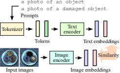
(a) Prompt-guided AD.

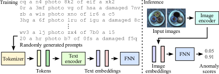
(b) Our method.

Figure 2: Overview of prompt-guided AD and our method.

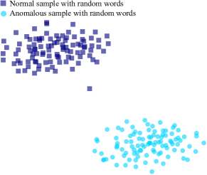
Figure 3: t-SNE plot of generated text embeddings.

To train an FNN-based anomaly detector, we generate training samples by feeding prompts into CLIP with random word data augmentation. Samples are generated based on two prompt templates, “[$\text{w}_{\text{0}}$] a [$\text{w}_{\text{1}}$] photo [$\text{w}_{\text{2}}$] of [$\text{w}_{\text{3}}$] [n] [$\text{w}_{\text{4}}$]” for normal samples and “[$\text{w}_{\text{5}}$] a [$\text{w}_{\text{6}}$] photo [$\text{w}_{\text{7}}$] of [$\text{w}_{\text{8}}$] [a] [$\text{w}_{\text{9}}$]” for anomalous samples. At the locations of “[n]” and “[a]”, words of normal and anomaly are inserted, respectively, in the same way as the prompt-guided AD. At the locations of “[$\text{w}_{\text{i}}$]”, randomly generated words are inserted.

Words for “[$\text{w}_{\text{i}}$]” are generated by randomly selecting letters from the English alphabet and digits. The length of each word is also randomly selected between the range from the minimum length $l_{min}$ to the maximum length $l_{max}$. The selected letters are concatenated and compose a single word. We insert individually generated words into the prompt templates and finally obtain prompts as depicted in Fig. 2 for generating training samples.

The completed prompts are transformed into text embeddings via the tokenizer and text encoder in CLIP. Suppose we have $N_{p}$ pairs of completed normal and anomalous prompts, a set of the pairs of tokens $\mathcal{T}=\{(\bm{t}_{i}^{(n)},\bm{t}_{i}^{(a)})\}_{i=1}^{N_{p}}$ is obtained, and then tokens $\bm{t}_{i}^{(n)}$ and $\bm{t}_{i}^{(a)}$ are transformed into text embeddings as $\bm{e}_{i}^{(n)}=f_{tenc}(\bm{t}_{i}^{(n)})$ and $\bm{e}_{i}^{(a)}=f_{tenc}(\bm{t}_{i}^{(a)})$. The obtained set of text embedding pairs $\mathcal{E}=\{(\bm{e}_{i}^{(n)},\bm{e}_{i}^{(a)})\}_{i=1}^{N_{p}}$ is used as a training set for anomaly detectors. We evaluate AD performances with several $N_{p}$ values, which are reported in Sec. 4.4.

The proposed data augmentation increases the diversity of training samples and thus enhances the performance of anomaly detectors. Figure 3 illustrates the t-SNE [van der Maaten and Hinton(2008)] plot of the generated text embeddings. It can be seen from the figure that normal and anomalous samples are separately distributed, while samples in either group of normal or anomaly have a certain amount of diversity. Since any object categories are specified in the prompts to generate training samples, the trained anomaly detector can be applied even when target object categories are unknown, resulting in obtaining category-agnostic anomaly detectors.

3.3 Training and Inference

As illustrated in Fig. 2, we use an FNN as an anomaly detector, which is trained with the generated text embeddings. During training, generated samples $\bm{e}_{i}^{(n)}$ and $\bm{e}_{i}^{(a)}$ are fed into an FNN, and the binary cross entropy loss is calculated, where normal and anomalous samples are labeled as 0 and 1, respectively. The samples of the same pair are always contained in the same batch because we empirically found that the performance was slightly improved with that strategy. During inference, an input image $I$ is first transformed into an image embedding $\bm{e}^{(i)}$ as $\bm{e}^{(i)}=f_{ienc}(I)$, and then an anomaly score $s_{FNN}$ is obtained as $s_{FNN}=\sigma(f_{FNN}(\bm{e}^{(i)}))$, where $f_{FNN}(\cdot)$ is the trained FNN and $\sigma(\cdot)$ is the sigmoid function. Since the text and image embeddings from CLIP have similar semantics due to the contrastive learning of CLIP, the trained FNN can be applied to the image embeddings even though the FNN is not trained with them. The obtained scores can solely be used to detect anomalous samples or can be combined with any kind of score such as $s_{pr}$ to enhance the performance.

4 Experiments

4.1 Datasets and Evaluation Metrics

To validate the effectiveness of the proposed method, we conduct extensive experiments on three publicly available benchmark datasets: the MVTec-AD [Bergmann et al.(2019)Bergmann, Fauser, Sattlegger, and Steger], VisA [Zou et al.(2022)Zou, Jeong, Pemula, Zhang, and Dabeer], and SewerML [Haurum and Moeslund(2021)] datasets. The former two datasets are common AD datasets. The MVTec-AD dataset includes 15 object categories, while the VisA dataset comprises 12 object categories. We use the SewerML dataset to evaluate the capability of detecting anomalous samples whose object categories are difficult to define due to their diversities. Although defect types are defined in the dataset, the appearance of each defect is not fixed and thus is challenging to classify, especially in a zero-shot manner. We compare CLIP [Radford et al.(2021)Radford, Kim, Hallacy, Ramesh, Goh, Agarwal, Sastry, Askell, Mishkin, Clark, Krueger, and Sutskever] and our method with this dataset to validate the effectiveness when ambiguous anomalous samples must be detected. Only the validation set of the SewerML dataset is used for this evaluation.

Following the work of WinCLIP [Jeong et al.(2023)Jeong, Zou, Kim, Zhang, Ravichandran, and Dabeer], we report the evaluation metrics of Area Under the Receiver Operating Characteristic (AUROC), Area Under the Precision-Recall curve (AUPR), and $F_{\text{1}}$-score at optimal threshold ($F_{\text{1}}$-max). The reported values of our method are the mean and standard deviation of trials with 10 random seeds.

4.2 Implementation Details

In all the experiments, we use OpenCLIP as the implementation of CLIP [Radford et al.(2021)Radford, Kim, Hallacy, Ramesh, Goh, Agarwal, Sastry, Askell, Mishkin, Clark, Krueger, and Sutskever] and the LAION-400M [Schuhmann et al.(2021)Schuhmann, Vencu, Beaumont, Kaczmarczyk, Mullis, Katta, Coombes, Jitsev, and Komatsuzaki]-based CLIP with ViT-B/16+ [Ilharco et al.(2021)Ilharco, Wortsman, Wightman, Gordon, Carlini, Taori, Dave, Shankar, Namkoong, Miller, Hajishirzi, Farhadi, and Schmidt], which is also used by the work of WinCLIP [Jeong et al.(2023)Jeong, Zou, Kim, Zhang, Ravichandran, and Dabeer], for fair comparisons. The FNN has four linear layers with batch normalization [Ioffe and Szegedy(2015)], ReLU activations, and dropout [Srivastava et al.(2014)Srivastava, Hinton, Krizhevsky, Sutskever, and Salakhutdinov]. The network is trained for 2 epochs using the AdamW [Loshchilov and Hutter(2019)] optimizer with a batch size of 128, the initial learning rate of $10^{-3}$ and the weight decay of $10^{-4}$. The learning rate is decayed after 1 epoch. Note that each batch comprises paired normal and anomalous samples as described in Sec. 3.3. Unless otherwise noted, we use multi-crop data augmentation at test time for both CLIP and our method because WinCLIP also uses the multi-crop strategy.

For the random word data augmentation, the minimum word length $l_{min}$ is set to 5, and the maximum word length $l_{max}$ is set to 10. By default, 10,000 pairs of normal and anomalous samples are generated with “a” for a word of normal and “a damaged” for a word of anomaly. The performances with other settings are analyzed in Sec. 4.4.

As denoted in Sec. 3.3, the scores of the FNN can be combined with other scores. In zero-shot setups, the performances with $s_{pr}+s_{FNN}$ (indicated by “CLIP + ours”) as well as with the individual score $s_{FNN}$ (indicated by “ours”) are reported. For future reference, we also report the performances of few-shot setups. In these setups, an additional score $s_{img}$ is calculated based on the similarities between the image embeddings of test samples and reference normal samples as described in the paper of WinCLIP. The performances are evaluated with the added score $s_{pr}+s_{FNN}+s_{img}$ (indicated by “CLIP + ours”).

4.3 Comparison against State of The Art

Table 1: Comparison against state-of-the-art methods.

		MVTec-AD			VisA
Setup	Method	AUROC	AUPR	$F_{1}$-max	AUROC	AUPR	$F_{1}$-max
0-shot $\left(\begin{array}[]{@{}c@{}}\text{Object}\\ \text{unknown}\end{array}\right)$	CLIP [Radford et al.(2021)Radford, Kim, Hallacy, Ramesh, Goh, Agarwal, Sastry, Askell, Mishkin, Clark, Krueger, and Sutskever]	91.5	95.7	92.0	76.5	80.5	78.1
2-8	Ours	91.0$\pm$0.4	95.4$\pm$0.3	92.2$\pm$0.3	78.1$\pm$1.1	81.3$\pm$0.9	79.8$\pm$0.4
	CLIP + ours	92.2$\pm$0.3	96.0$\pm$0.2	92.8$\pm$0.2	78.2$\pm$0.8	81.5$\pm$0.8	79.9$\pm$0.3
0-shot $\left(\begin{array}[]{@{}c@{}}\text{Object}\\ \text{known}\end{array}\right)$	WinCLIP [Jeong et al.(2023)Jeong, Zou, Kim, Zhang, Ravichandran, and Dabeer]	91.8	96.5	92.9	78.1	81.2	79.0
	CLIP [Radford et al.(2021)Radford, Kim, Hallacy, Ramesh, Goh, Agarwal, Sastry, Askell, Mishkin, Clark, Krueger, and Sutskever]	92.6	96.3	93.0	76.3	80.4	78.8
2-8	CLIP + ours	93.0$\pm$0.3	96.4$\pm$0.2	93.1$\pm$0.2	79.8$\pm$0.6	82.8$\pm$0.6	79.9$\pm$0.2
1-shot	SPADE [Cohen and Hoshen(2020)]	81.0$\pm$2.0	90.6$\pm$0.8	90.3$\pm$0.8	79.5$\pm$4.0	82.0$\pm$3.3	80.7$\pm$1.9
	PaDiM [Defard et al.(2021)Defard, Setkov, Loesch, and Audigier]	76.6$\pm$3.1	88.1$\pm$1.7	88.2$\pm$1.1	62.8$\pm$5.4	68.3$\pm$4.0	75.3$\pm$1.2
	PatchCore [Roth et al.(2022)Roth, Pemula, Zepeda, Schölkopf, Brox, and Gehler]	83.4$\pm$3.0	92.2$\pm$1.5	90.5$\pm$1.5	79.9$\pm$2.9	82.8$\pm$2.3	81.7$\pm$1.6
	WinCLIP [Jeong et al.(2023)Jeong, Zou, Kim, Zhang, Ravichandran, and Dabeer]	93.1$\pm$2.0	96.5$\pm$0.9	93.7$\pm$1.1	83.8$\pm$4.0	85.1$\pm$4.0	83.1$\pm$1.7
2-8	CLIP + ours	93.3$\pm$0.5	96.7$\pm$0.2	94.0$\pm$0.3	83.4$\pm$1.7	85.8$\pm$1.8	83.6$\pm$0.8
2-shot	SPADE [Cohen and Hoshen(2020)]	82.9$\pm$2.6	91.7$\pm$1.2	91.1$\pm$1.0	80.7$\pm$5.0	82.3$\pm$4.3	81.7$\pm$2.5
	PaDiM [Defard et al.(2021)Defard, Setkov, Loesch, and Audigier]	78.9$\pm$3.1	89.3$\pm$1.7	89.2$\pm$1.1	67.4$\pm$5.1	71.6$\pm$3.8	75.7$\pm$1.8
	PatchCore [Roth et al.(2022)Roth, Pemula, Zepeda, Schölkopf, Brox, and Gehler]	86.3$\pm$3.3	93.8$\pm$1.7	92.0$\pm$1.5	81.6$\pm$4.0	84.8$\pm$3.2	82.5$\pm$1.8
	RegAD [Huang et al.(2022)Huang, Guan, Jiang, Zhang, Spratlin, and Wang]	85.7	–	–	–	–	–
	WinCLIP [Jeong et al.(2023)Jeong, Zou, Kim, Zhang, Ravichandran, and Dabeer]	94.4$\pm$1.3	97.0$\pm$0.7	94.4$\pm$0.8	84.6$\pm$2.4	85.8$\pm$2.7	83.0$\pm$1.4
2-8	CLIP + ours	94.0$\pm$0.7	96.9$\pm$0.3	94.1$\pm$0.3	85.6$\pm$1.4	87.5$\pm$1.6	84.1$\pm$1.0
4-shot	SPADE [Cohen and Hoshen(2020)]	84.8$\pm$2.5	92.5$\pm$1.2	91.5$\pm$0.9	81.7$\pm$3.4	83.4$\pm$2.7	82.1$\pm$2.1
	PaDiM [Defard et al.(2021)Defard, Setkov, Loesch, and Audigier]	80.4$\pm$2.5	90.5$\pm$1.6	90.2$\pm$1.2	72.8$\pm$2.9	75.6$\pm$2.2	78.0$\pm$1.2
	PatchCore [Roth et al.(2022)Roth, Pemula, Zepeda, Schölkopf, Brox, and Gehler]	88.8$\pm$2.6	94.5$\pm$1.5	92.6$\pm$1.6	85.3$\pm$2.1	87.5$\pm$2.1	84.3$\pm$1.3
	RegAD [Huang et al.(2022)Huang, Guan, Jiang, Zhang, Spratlin, and Wang]	88.2	–	–	–	–	–
	WinCLIP [Jeong et al.(2023)Jeong, Zou, Kim, Zhang, Ravichandran, and Dabeer]	95.2$\pm$1.3	97.3$\pm$0.6	94.7$\pm$0.8	87.3$\pm$1.8	88.8$\pm$1.8	84.2$\pm$1.6
2-8	CLIP + ours	94.5$\pm$0.7	97.1$\pm$0.3	94.4$\pm$0.3	86.6$\pm$0.9	88.4$\pm$1.3	84.5$\pm$0.6

We compare our method against state-of-the-art zero/few-shot AD methods. Table 4.3 shows the comparison results. For zero-shot AD, we evaluate performances in two setups. One is an unknown-object setup, where we assume that target object categories are unknown and thus a word “object” is used in CLIP’s prompts. The other is known-object setup, where we assume that target object categories are known and thus inserted into CLIP’s prompts. As can be seen in the table, our method outperforms CLIP’s [Radford et al.(2021)Radford, Kim, Hallacy, Ramesh, Goh, Agarwal, Sastry, Askell, Mishkin, Clark, Krueger, and Sutskever] prompt-guided AD and WinCLIP [Jeong et al.(2023)Jeong, Zou, Kim, Zhang, Ravichandran, and Dabeer] with almost all the evaluation metrics when combined with CLIP. In particular, the performance gaps between the existing and our methods are larger in the zero-shot unknown-object setup than in the known-object setup, which indicates the effectiveness of detecting ambiguous anomalous samples.

The performances of the few-shot setups show that our method achieves competitive performances even when some normal reference images are provided. These results suggest that our method can be combined with state-of-the-art methods and enhance their performance.

Table 2: Comparison against state-of-the-art methods without multiple crops on the MVTec-AD dataset in the zero-shot known-object setup.

Method	Prompt ens.	AUROC	AUPR	$F_{1}$-max
WinCLIP [Jeong et al.(2023)Jeong, Zou, Kim, Zhang, Ravichandran, and Dabeer]	✓	90.8	96.1	92.5
CLIP [Radford et al.(2021)Radford, Kim, Hallacy, Ramesh, Goh, Agarwal, Sastry, Askell, Mishkin, Clark, Krueger, and Sutskever]		89.8	95.4	92.1
Ours		89.6$\pm$0.6	95.5$\pm$0.2	91.5$\pm$0.3
CLIP + ours		91.0$\pm$0.3	96.2$\pm$0.2	92.5$\pm$0.2

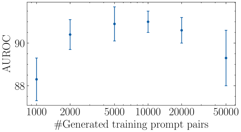
Figure 4: AUROCs with the various numbers of training prompt pairs in the zero-shot unknown-object setup.

We also compare the performances of CLIP [Radford et al.(2021)Radford, Kim, Hallacy, Ramesh, Goh, Agarwal, Sastry, Askell, Mishkin, Clark, Krueger, and Sutskever], WinCLIP [Jeong et al.(2023)Jeong, Zou, Kim, Zhang, Ravichandran, and Dabeer], and our method without the multi-crop strategy. If the multi-crop is eliminated from WinCLIP, the performance purely depends on the prompt ensembling, which is a suitable baseline to evaluate the capability of our method. Table 2 shows the comparison results. As shown in the table, our method achieves better performance than WinCLIP. The results indicate that our random word data augmentation can improve performance better than prompt ensembling.

4.4 Analysis on Data Augmention

We first analyze the effect of the number of prompt pairs $N_{p}$ for training the FNN. Figure 4.3 shows the performances on the MVTec-AD dataset with regard to the different values of $N_{p}$ in the unknown-object setup. As shown in the figure, the best performance is achieved when $N_{p}$ is 10,000, and fewer or more pairs degrade the performance. The lower performance with fewer samples is attributed to insufficient training data, and that with more samples is probably due to over-fitting. As analyzed in Sec. 4.5, embeddings generated from our random data augmentation have a different distribution from that of the embeddings generated from natural sentences. A large number of such training samples force models to have an incorrect decision boundary and thus degrades the performance.

Table 3: AUROCs with various word pairs for normal and anomaly in the zero-shot unknown-object setup. The left value in each cell is the result of CLIP [Radford et al.(2021)Radford, Kim, Hallacy, Ramesh, Goh, Agarwal, Sastry, Askell, Mishkin, Clark, Krueger, and Sutskever], and the right value is that of CLIP + ours.

	“a damaged”	“a broken”	“a defective”	“an anomalous”
“an”	91.5$\diagup$92.2$\pm$0.3	87.5$\diagup$86.1$\pm$0.6	79.4$\diagup$85.7$\pm$0.5	67.6$\diagup$73.7$\pm$0.3
“a normal”	89.3$\diagup$90.5$\pm$0.2	87.3$\diagup$88.6$\pm$0.5	81.8$\diagup$84.5$\pm$0.9	69.1$\diagup$71.9$\pm$1.0
“a good”	88.4$\diagup$89.6$\pm$0.3	86.1$\diagup$87.0$\pm$0.5	80.6$\diagup$86.3$\pm$0.4	68.6$\diagup$73.0$\pm$0.9
“a flawless”	88.5$\diagup$90.3$\pm$0.4	85.7$\diagup$86.0$\pm$0.8	77.7$\diagup$84.5$\pm$0.6	68.8$\diagup$75.8$\pm$0.5

We then analyze the effect of normal and anomaly word choices in guiding prompts and prompt templates. Table 3 shows the evaluation results of CLIP$\diagup$CLIP + ours. Each row and column shows the performances with the indicated word as normal and anomaly in the prompts. As illustrated in the table, our method improves the performances of CLIP with any word pairs except for the pair of “an” and “a broken”. In particular, our method significantly improves performances in the case where word pairs are inappropriate for CLIP. The results suggest that our method can show word-agnostic performance improvement and can boost the robustness of the prompt-guided AD.

4.5 Analysis on Feature Embeddings

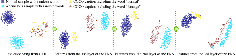
Figure 5: t-SNE plots of feature embeddings from different layers.

To analyze how the FNN learns to classify normal and anomalous samples with our random word data augmentation, we obtain natural sentences that contain a word of either “normal” or “damage” from COCO captions [Lin et al.(2014)Lin, Maire, Belongie, Hays, Perona, Ramanan, Dollár, and Zitnick] and plot the embeddings of those natural sentences in addition to the augmented prompts with t-SNE [van der Maaten and Hinton(2008)]. Figure 5 shows the plotted results. As shown in the figure, CLIP’s embeddings of the natural sentences and augmented prompts have different domains. However, the embeddings from the FNN layers are gradually split by their sample types rather than their domains. These plots indicate that the trained FNN learns to extract features containing information on normality and thus successfully classifies anomalous samples of arbitrary object categories.

4.6 Potential Application

Table 4: Comparison of CLIP and our method on the SewerML dataset.

Method	AUROC	AUPR	$F_{1}$-max
CLIP [Radford et al.(2021)Radford, Kim, Hallacy, Ramesh, Goh, Agarwal, Sastry, Askell, Mishkin, Clark, Krueger, and Sutskever]	79.1	77.7	75.2
Ours	82.6$\pm$1.3	81.0$\pm$1.3	77.4$\pm$0.9
CLIP + Ours	81.7$\pm$0.9	80.2$\pm$0.7	76.9$\pm$0.8

To validate the effectiveness of our method in detecting ambiguous anomalous samples, we evaluate the performances of CLIP [Radford et al.(2021)Radford, Kim, Hallacy, Ramesh, Goh, Agarwal, Sastry, Askell, Mishkin, Clark, Krueger, and Sutskever] and our method on the SewerML dataset [Haurum and Moeslund(2021)]. Table 4.6 shows the comparison results. As shown in the table, our method without the prompt-guided AD achieves the best performance among the three methods. The reason for the best performance without the prompt-guided AD is probably because CLIP cannot handle the diversity of defects in the dataset and thus degrades the performance rather than improving it. In contrast, our FNN is trained with a diverse set of normal and anomalous samples and thus can achieve better performance.

5 Conclusion

We propose a novel zero-shot category-agnostic AD method that leverages CLIP as a data source for training anomaly detectors. Our method differs from existing methods in that our method does not include object categories in prompts to generate training samples and thus can be applied to the case where object categories are unknown. Furthermore, training samples generated by our method are so diverse that our method can achieve significant performance even without prompt ensembling. We perform extensive experiments and show the effectiveness of our method.

A Detailed Quantitative Results

We report category-wise performance of CLIP [Radford et al.(2021)Radford, Kim, Hallacy, Ramesh, Goh, Agarwal, Sastry, Askell, Mishkin, Clark, Krueger, and Sutskever], WinCLIP [Jeong et al.(2023)Jeong, Zou, Kim, Zhang, Ravichandran, and Dabeer], and ours for future reference. Our performances are those with the score combination of CLIP and our trained feed-forward network. The reported values of our method are the mean and standard deviation of trials with 10 random seeds.

Table 5: Class-wise AUROC on the MVTec-AD dataset.

	0-shot $\left(\begin{array}[]{@{}c@{}}\text{Object}\\ \text{unknown}\end{array}\right)$		0-shot $\left(\begin{array}[]{@{}c@{}}\text{Object}\\ \text{known}\end{array}\right)$
					1-shot		2-shot		4-shot
Category	CLIP	CLIP + ours	WinCLIP	CLIP + ours	WinCLIP	CLIP + ours	WinCLIP	CLIP + ours	WinCLIP	CLIP + ours
Bottle	99.4	97.1$\pm$1.1	99.2	97.0$\pm$0.8	98.2$\pm$0.9	97.8$\pm$0.6	99.3$\pm$0.3	98.1$\pm$0.7	99.3$\pm$0.4	98.2$\pm$0.6
Cable	83.0	84.2$\pm$0.6	86.5	86.4$\pm$1.4	88.9$\pm$1.9	90.8$\pm$1.1	88.4$\pm$0.7	91.3$\pm$2.0	90.9$\pm$0.9	92.1$\pm$0.8
Capsule	85.3	87.3$\pm$2.0	72.9	88.7$\pm$2.8	72.3$\pm$6.8	76.8$\pm$6.4	77.3$\pm$8.8	83.6$\pm$7.1	82.3$\pm$8.9	87.8$\pm$7.9
Carpet	100	100$\pm$0.0	100	100$\pm$0.0	99.8$\pm$0.3	100$\pm$0.0	99.8$\pm$0.3	100$\pm$0.0	100$\pm$0.0	100$\pm$0.0
Grid	99.2	99.0$\pm$0.4	98.8	98.7$\pm$0.2	99.5$\pm$0.3	99.2$\pm$0.5	99.4$\pm$0.2	99.1$\pm$0.4	99.6$\pm$0.1	99.6$\pm$0.2
Hazelnut	92.0	94.3$\pm$1.1	93.9	94.0$\pm$0.5	97.5$\pm$1.4	94.9$\pm$0.6	98.3$\pm$0.7	95.0$\pm$0.5	98.4$\pm$0.4	95.1$\pm$0.5
Leather	100	100$\pm$0.0	100	100$\pm$0.0	99.9$\pm$0.0	100$\pm$0.0	99.9$\pm$0.0	99.9$\pm$0.0	100$\pm$0.0	100$\pm$0.0
Metal nut	94.4	96.1$\pm$1.3	97.1	94.7$\pm$1.7	98.7$\pm$0.8	96.1$\pm$1.3	99.4$\pm$0.2	96.1$\pm$1.4	99.5$\pm$0.2	96.3$\pm$1.3
Pill	88.3	88.6$\pm$1.6	79.1	90.2$\pm$1.0	91.2$\pm$2.1	92.5$\pm$1.3	92.3$\pm$0.7	92.6$\pm$1.2	92.8$\pm$1.0	92.6$\pm$1.3
Screw	76.1	76.6$\pm$1.5	83.3	75.5$\pm$2.1	86.4$\pm$0.9	77.4$\pm$1.8	86.0$\pm$2.1	77.5$\pm$2.1	87.9$\pm$1.2	77.6$\pm$2.1
Tile	99.4	99.5$\pm$0.2	100	99.5$\pm$0.2	99.9$\pm$0.0	99.6$\pm$0.1	99.9$\pm$0.2	99.6$\pm$0.1	99.9$\pm$0.1	99.6$\pm$0.1
Toothbrush	92.8	88.4$\pm$3.5	87.5	94.0$\pm$0.9	92.2$\pm$4.9	94.7$\pm$1.3	97.5$\pm$1.6	95.0$\pm$1.0	96.7$\pm$2.6	96.4$\pm$1.5
Transistor	79.7	86.6$\pm$1.4	88.0	88.9$\pm$1.3	83.4$\pm$3.8	89.4$\pm$1.3	85.3$\pm$1.7	89.6$\pm$1.4	85.7$\pm$2.5	89.6$\pm$1.3
Wood	97.8	97.6$\pm$0.6	99.4	98.1$\pm$0.5	99.9$\pm$0.1	98.7$\pm$0.6	99.9$\pm$0.1	98.8$\pm$0.5	99.8$\pm$0.3	98.8$\pm$0.6
Zipper	85.5	87.4$\pm$1.0	91.5	88.8$\pm$0.1	88.8$\pm$5.9	91.6$\pm$2.9	94.0$\pm$1.4	93.8$\pm$1.0	94.5$\pm$0.5	94.3$\pm$1.0

Table 6: Class-wise AUPR on the MVTec-AD dataset.

	0-shot $\left(\begin{array}[]{@{}c@{}}\text{Object}\\ \text{unknown}\end{array}\right)$		0-shot $\left(\begin{array}[]{@{}c@{}}\text{Object}\\ \text{known}\end{array}\right)$
					1-shot		2-shot		4-shot
Category	CLIP	CLIP + ours	WinCLIP	CLIP + ours	WinCLIP	CLIP + ours	WinCLIP	CLIP + ours	WinCLIP	CLIP + ours
Bottle	99.8	99.2$\pm$0.3	99.8	99.2$\pm$0.2	99.4$\pm$0.3	99.4$\pm$0.2	99.8$\pm$0.1	99.4$\pm$0.2	99.8$\pm$0.1	99.5$\pm$0.2
Cable	88.3	89.3$\pm$0.5	91.2	91.6$\pm$1.0	93.2$\pm$1.1	94.6$\pm$0.8	92.9$\pm$0.6	94.9$\pm$1.2	94.4$\pm$0.3	95.4$\pm$0.5
Capsule	96.8	96.8$\pm$0.7	91.5	97.0$\pm$0.9	91.6$\pm$2.7	93.4$\pm$2.2	93.3$\pm$3.6	95.6$\pm$2.2	95.1$\pm$3.3	96.6$\pm$2.6
Carpet	100	100$\pm$0.0	100	100$\pm$0.0	99.9$\pm$0.1	100$\pm$0.0	99.9$\pm$0.1	100$\pm$0.0	100$\pm$0.0	100$\pm$0.0
Grid	99.7	99.7$\pm$0.1	99.6	99.6$\pm$0.0	99.9$\pm$0.1	99.7$\pm$0.2	99.8$\pm$0.1	99.7$\pm$0.1	99.9$\pm$0.0	99.9$\pm$0.1
Hazelnut	96.0	96.7$\pm$0.6	96.9	96.2$\pm$0.4	98.6$\pm$0.7	96.8$\pm$0.5	99.1$\pm$0.4	96.8$\pm$0.4	99.1$\pm$0.2	96.9$\pm$0.5
Leather	100	100$\pm$0.0	100	100$\pm$0.0	100$\pm$0.0	100$\pm$0.0	100$\pm$0.0	100$\pm$0.0	100$\pm$0.0	100$\pm$0.0
Metal nut	98.8	99.1$\pm$0.3	99.3	98.8$\pm$0.4	99.7$\pm$0.2	99.1$\pm$0.3	99.9$\pm$0.0	99.1$\pm$0.3	99.9$\pm$0.1	99.2$\pm$0.3
Pill	97.5	97.6$\pm$0.4	95.7	98.0$\pm$0.2	98.3$\pm$0.5	98.5$\pm$0.3	98.6$\pm$0.1	98.5$\pm$0.3	98.6$\pm$0.2	98.5$\pm$0.3
Screw	90.3	90.7$\pm$0.8	93.1	90.1$\pm$1.2	94.2$\pm$0.6	91.0$\pm$1.1	94.1$\pm$1.5	91.1$\pm$1.1	94.9$\pm$0.8	91.1$\pm$1.1
Tile	99.8	99.8$\pm$0.1	100	99.8$\pm$0.1	100$\pm$0.0	99.8$\pm$0.1	100$\pm$0.1	99.8$\pm$0.0	100$\pm$0.0	99.8$\pm$0.1
Toothbrush	97.7	95.4$\pm$1.7	95.6	97.6$\pm$0.4	96.7$\pm$2.0	97.9$\pm$0.6	99.0$\pm$0.6	98.0$\pm$0.4	98.7$\pm$1.1	98.6$\pm$0.6
Transistor	76.5	80.4$\pm$1.7	87.1	82.3$\pm$2.1	79.0$\pm$4.0	83.3$\pm$2.1	80.7$\pm$2.3	83.5$\pm$2.2	80.7$\pm$3.2	83.6$\pm$2.1
Wood	99.3	99.3$\pm$0.2	99.8	99.4$\pm$0.2	100$\pm$0.0	99.6$\pm$0.2	100$\pm$0.0	99.6$\pm$0.2	99.9$\pm$0.1	99.6$\pm$0.2
Zipper	95.6	96.1$\pm$0.3	97.5	96.7$\pm$0.0	96.8$\pm$1.8	97.5$\pm$0.9	98.3$\pm$0.4	98.1$\pm$0.4	98.5$\pm$0.2	98.3$\pm$0.3

Table 7: Class-wise $F_{1}$-max on the MVTec-AD dataset.

	0-shot $\left(\begin{array}[]{@{}c@{}}\text{Object}\\ \text{unknown}\end{array}\right)$		0-shot $\left(\begin{array}[]{@{}c@{}}\text{Object}\\ \text{known}\end{array}\right)$
					1-shot		2-shot		4-shot
Category	CLIP	CLIP + ours	WinCLIP	CLIP + ours	WinCLIP	CLIP + ours	WinCLIP	CLIP + ours	WinCLIP	CLIP + ours
Bottle	98.4	95.2$\pm$1.1	97.6	95.9$\pm$0.7	96.5$\pm$1.3	96.5$\pm$0.6	97.7$\pm$0.7	96.6$\pm$0.7	97.8$\pm$0.6	96.6$\pm$0.7
Cable	84.5	85.7$\pm$0.8	84.5	84.4$\pm$1.2	86.1$\pm$1.3	87.7$\pm$1.0	85.2$\pm$0.7	87.6$\pm$2.0	87.2$\pm$0.6	87.8$\pm$1.0
Capsule	90.7	92.6$\pm$0.8	91.4	93.3$\pm$0.8	91.6$\pm$0.7	93.1$\pm$0.7	92.1$\pm$0.7	94.0$\pm$0.8	92.5$\pm$0.5	94.7$\pm$0.8
Carpet	99.4	99.6$\pm$0.4	99.4	99.6$\pm$0.4	99.2$\pm$0.8	100$\pm$0.0	99.3$\pm$0.7	100$\pm$0.0	99.9$\pm$0.2	100$\pm$0.0
Grid	97.3	97.8$\pm$0.6	98.2	97.3$\pm$0.0	98.9$\pm$0.4	98.1$\pm$0.7	99.1$\pm$0.0	98.1$\pm$0.5	99.1$\pm$0.0	98.4$\pm$0.4
Hazelnut	88.9	91.9$\pm$1.7	89.7	91.8$\pm$1.0	94.7$\pm$2.3	92.7$\pm$0.9	95.6$\pm$1.6	92.9$\pm$0.8	96.2$\pm$1.0	93.0$\pm$0.8
Leather	100	100$\pm$0.0	100	100$\pm$0.0	99.5$\pm$0.0	99.7$\pm$0.3	99.7$\pm$0.2	99.5$\pm$0.3	99.8$\pm$0.2	99.9$\pm$0.2
Metal nut	93.3	95.0$\pm$1.1	96.3	94.0$\pm$1.2	97.7$\pm$1.0	95.0$\pm$1.0	98.4$\pm$0.5	94.9$\pm$1.2	98.5$\pm$0.6	95.1$\pm$1.0
Pill	93.7	93.4$\pm$0.6	91.6	93.9$\pm$0.3	93.8$\pm$0.7	95.1$\pm$0.7	94.3$\pm$0.4	95.2$\pm$0.7	94.1$\pm$0.4	95.1$\pm$0.8
Screw	86.9	86.9$\pm$0.0	87.4	86.9$\pm$0.2	88.5$\pm$0.3	86.9$\pm$0.3	89.0$\pm$0.6	87.0$\pm$0.4	89.6$\pm$0.7	87.0$\pm$0.4
Tile	97.7	97.8$\pm$0.6	99.4	97.8$\pm$0.6	98.9$\pm$0.2	97.9$\pm$0.5	99.2$\pm$0.3	97.9$\pm$0.5	99.2$\pm$0.3	98.0$\pm$0.5
Toothbrush	93.1	90.2$\pm$0.9	87.9	92.7$\pm$0.7	94.1$\pm$1.9	94.1$\pm$1.1	96.7$\pm$1.8	93.7$\pm$0.9	96.8$\pm$2.3	95.3$\pm$1.6
Transistor	69.7	79.6$\pm$1.8	79.5	81.7$\pm$1.5	75.1$\pm$3.1	81.6$\pm$1.7	75.9$\pm$2.4	81.7$\pm$1.7	76.6$\pm$2.8	81.8$\pm$1.5
Wood	95.7	95.8$\pm$0.6	98.3	96.0$\pm$0.4	99.4$\pm$0.3	97.2$\pm$0.6	99.5$\pm$0.4	97.2$\pm$0.6	99.2$\pm$0.9	97.1$\pm$0.7
Zipper	90.0	91.2$\pm$0.8	92.9	91.9$\pm$0.1	92.1$\pm$2.5	93.7$\pm$2.1	94.4$\pm$0.3	95.5$\pm$0.3	94.7$\pm$0.4	95.5$\pm$0.3

Table 8: Class-wise AUROC on the VisA dataset.

	0-shot $\left(\begin{array}[]{@{}c@{}}\text{Object}\\ \text{unknown}\end{array}\right)$		0-shot $\left(\begin{array}[]{@{}c@{}}\text{Object}\\ \text{known}\end{array}\right)$
					1-shot		2-shot		4-shot
Category	CLIP	CLIP + ours	WinCLIP	CLIP + ours	WinCLIP	CLIP + ours	WinCLIP	CLIP + ours	WinCLIP	CLIP + ours
Candle	96.0	96.9$\pm$0.3	95.4	97.0$\pm$0.1	93.4$\pm$1.4	97.7$\pm$0.2	94.8$\pm$1.0	97.9$\pm$0.1	95.1$\pm$0.3	97.9$\pm$0.2
Capsules	74.9	78.1$\pm$2.3	85.0	75.6$\pm$0.3	85.0$\pm$3.1	82.1$\pm$0.6	84.9$\pm$0.8	82.5$\pm$0.6	86.8$\pm$1.7	82.6$\pm$0.6
Cashew	87.3	91.6$\pm$2.4	92.1	91.8$\pm$1.0	94.0$\pm$0.4	92.9$\pm$1.1	94.3$\pm$0.5	93.1$\pm$0.8	95.2$\pm$0.8	93.1$\pm$0.8
Chewing gum	89.8	94.3$\pm$1.3	96.5	93.0$\pm$1.9	97.6$\pm$0.8	95.0$\pm$0.7	97.3$\pm$0.8	95.1$\pm$0.7	97.7$\pm$0.3	95.3$\pm$0.6
Fryum	88.2	90.0$\pm$0.5	80.3	89.2$\pm$0.5	88.5$\pm$1.9	92.6$\pm$1.2	90.5$\pm$0.4	92.8$\pm$1.3	90.8$\pm$0.5	92.9$\pm$1.2
Macaroni1	82.0	82.5$\pm$2.0	76.2	89.4$\pm$1.4	82.9$\pm$1.5	91.5$\pm$1.7	83.3$\pm$1.9	91.5$\pm$1.7	85.2$\pm$0.9	91.6$\pm$1.6
Macaroni2	65.6	71.3$\pm$1.5	63.7	68.6$\pm$1.5	70.2$\pm$0.9	69.8$\pm$1.5	71.8$\pm$2.0	69.9$\pm$1.4	70.9$\pm$2.2	69.9$\pm$1.3
PCB1	58.2	49.7$\pm$7.0	73.6	69.4$\pm$3.8	75.6$\pm$23.0	70.7$\pm$16.9	76.7$\pm$5.2	80.2$\pm$10.4	88.3$\pm$1.7	83.1$\pm$2.5
PCB2	51.6	50.7$\pm$1.0	51.2	47.3$\pm$0.1	62.2$\pm$3.9	60.7$\pm$2.2	62.6$\pm$3.7	63.8$\pm$1.9	67.5$\pm$2.6	66.4$\pm$1.5
PCB3	66.0	67.9$\pm$1.3	73.4	66.3$\pm$0.4	74.1$\pm$1.1	74.0$\pm$8.4	78.8$\pm$1.9	80.3$\pm$3.4	83.3$\pm$1.7	83.4$\pm$1.8
PCB4	74.5	75.2$\pm$0.7	79.6	82.9$\pm$0.4	85.2$\pm$8.9	88.1$\pm$9.0	82.3$\pm$9.9	87.6$\pm$10.4	87.6$\pm$8.0	89.7$\pm$10.1
Pipe fryum	84.1	89.9$\pm$1.4	69.7	87.2$\pm$2.6	97.2$\pm$1.1	92.6$\pm$1.7	98.0$\pm$0.6	93.0$\pm$1.8	98.5$\pm$0.4	93.2$\pm$1.8

Table 9: Class-wise AUPR on the VisA dataset.

	0-shot $\left(\begin{array}[]{@{}c@{}}\text{Object}\\ \text{unknown}\end{array}\right)$		0-shot $\left(\begin{array}[]{@{}c@{}}\text{Object}\\ \text{known}\end{array}\right)$
					1-shot		2-shot		4-shot
Category	CLIP	CLIP + ours	WinCLIP	CLIP + ours	WinCLIP	CLIP + ours	WinCLIP	CLIP + ours	WinCLIP	CLIP + ours
Candle	96.3	96.9$\pm$0.3	95.8	96.9$\pm$0.2	93.6$\pm$1.5	97.6$\pm$0.2	95.1$\pm$1.1	97.7$\pm$0.1	95.3$\pm$0.4	97.8$\pm$0.1
Capsules	83.1	85.4$\pm$1.5	90.9	84.8$\pm$0.1	89.9$\pm$2.5	88.6$\pm$0.4	88.9$\pm$0.7	88.9$\pm$0.3	91.5$\pm$1.4	89.0$\pm$0.3
Cashew	94.3	96.2$\pm$1.0	96.4	96.3$\pm$0.4	97.2$\pm$0.2	96.9$\pm$0.4	97.3$\pm$0.2	96.9$\pm$0.3	97.7$\pm$0.4	96.9$\pm$0.3
Chewing gum	95.6	97.7$\pm$0.6	98.6	97.0$\pm$0.9	99.0$\pm$0.3	97.9$\pm$0.3	98.9$\pm$0.3	98.0$\pm$0.3	99.0$\pm$0.1	98.0$\pm$0.2
Fryum	94.8	95.7$\pm$0.2	90.1	95.4$\pm$0.3	94.7$\pm$1.0	97.0$\pm$0.5	95.8$\pm$0.2	97.0$\pm$0.6	96.0$\pm$0.3	97.1$\pm$0.6
Macaroni1	85.0	84.5$\pm$1.7	75.8	90.1$\pm$1.1	84.9$\pm$1.2	92.0$\pm$1.4	84.7$\pm$1.5	92.0$\pm$1.4	86.5$\pm$0.6	92.1$\pm$1.3
Macaroni2	60.8	67.4$\pm$1.6	60.3	66.3$\pm$1.9	68.4$\pm$1.8	68.5$\pm$1.6	70.4$\pm$1.8	68.9$\pm$1.7	69.6$\pm$2.8	68.9$\pm$1.7
PCB1	63.6	55.3$\pm$6.3	78.4	71.9$\pm$4.0	76.5$\pm$19.0	72.4$\pm$13.8	78.3$\pm$4.3	80.0$\pm$8.8	87.7$\pm$1.7	82.4$\pm$2.6
PCB2	54.9	54.0$\pm$0.7	49.2	49.6$\pm$0.1	64.9$\pm$3.3	64.7$\pm$2.1	65.8$\pm$4.0	68.0$\pm$1.5	71.3$\pm$3.4	70.1$\pm$0.7
PCB3	66.4	69.6$\pm$1.3	76.5	67.3$\pm$0.3	73.5$\pm$1.6	74.6$\pm$8.7	80.9$\pm$1.6	82.5$\pm$3.0	84.8$\pm$1.8	85.4$\pm$1.4
PCB4	79.6	79.9$\pm$0.5	77.7	84.4$\pm$0.4	78.5$\pm$15.5	83.2$\pm$13.7	72.5$\pm$16.2	83.6$\pm$14.4	85.6$\pm$8.9	86.0$\pm$14.6
Pipe fryum	91.6	95.1$\pm$0.8	82.3	93.6$\pm$2.1	98.6$\pm$0.5	96.2$\pm$1.1	99.0$\pm$0.3	96.4$\pm$1.1	99.2$\pm$0.2	96.5$\pm$1.1

Table 10: Class-wise $F_{1}$-max on the VisA dataset.

	0-shot $\left(\begin{array}[]{@{}c@{}}\text{Object}\\ \text{unknown}\end{array}\right)$		0-shot $\left(\begin{array}[]{@{}c@{}}\text{Object}\\ \text{known}\end{array}\right)$
					1-shot		2-shot		4-shot
Category	CLIP	CLIP + ours	WinCLIP	CLIP + ours	WinCLIP	CLIP + ours	WinCLIP	CLIP + ours	WinCLIP	CLIP + ours
Candle	91.1	92.4$\pm$0.6	89.4	92.2$\pm$0.3	87.8$\pm$1.2	94.7$\pm$0.5	89.1$\pm$1.3	95.2$\pm$0.4	88.9$\pm$1.0	95.1$\pm$0.3
Capsules	79.8	81.4$\pm$1.3	83.9	79.3$\pm$0.2	84.9$\pm$2.0	82.8$\pm$0.6	85.4$\pm$0.6	83.0$\pm$0.6	86.0$\pm$0.9	83.1$\pm$0.5
Cashew	84.3	89.0$\pm$2.3	88.4	89.1$\pm$1.2	90.7$\pm$0.7	89.6$\pm$1.3	90.9$\pm$0.7	89.8$\pm$1.0	91.6$\pm$1.3	90.0$\pm$1.0
Chewing gum	87.4	92.9$\pm$1.7	94.8	90.2$\pm$2.4	95.6$\pm$0.9	92.7$\pm$1.0	95.4$\pm$0.6	93.0$\pm$0.9	95.7$\pm$0.5	93.4$\pm$0.6
Fryum	86.2	87.6$\pm$0.8	82.7	86.9$\pm$0.9	87.2$\pm$1.4	91.0$\pm$2.0	88.4$\pm$0.6	91.0$\pm$1.9	88.9$\pm$0.8	91.4$\pm$1.9
Macaroni1	74.4	76.7$\pm$1.1	74.2	83.1$\pm$1.2	76.2$\pm$1.4	84.9$\pm$1.5	76.7$\pm$2.0	84.8$\pm$1.5	78.2$\pm$1.2	84.9$\pm$1.6
Macaroni2	71.9	71.6$\pm$1.1	69.8	69.4$\pm$0.7	72.3$\pm$1.1	70.1$\pm$0.9	73.9$\pm$0.9	69.9$\pm$0.7	73.1$\pm$1.6	70.0$\pm$0.7
PCB1	66.7	66.7$\pm$0.0	71.0	69.2$\pm$1.1	81.3$\pm$6.6	75.6$\pm$6.9	73.2$\pm$3.7	78.7$\pm$4.8	83.1$\pm$2.2	78.5$\pm$2.3
PCB2	67.1	67.2$\pm$0.2	67.1	67.1$\pm$0.1	67.2$\pm$0.3	68.1$\pm$0.8	67.3$\pm$0.3	68.5$\pm$0.5	67.7$\pm$0.6	69.3$\pm$0.8
PCB3	70.5	69.9$\pm$0.9	71.0	68.9$\pm$0.3	73.5$\pm$1.5	72.7$\pm$3.4	73.9$\pm$1.3	75.3$\pm$2.0	77.0$\pm$1.4	76.9$\pm$1.8
PCB4	73.3	74.3$\pm$0.6	74.9	77.0$\pm$0.5	86.1$\pm$2.1	89.6$\pm$3.9	86.8$\pm$3.8	88.4$\pm$6.6	84.6$\pm$7.0	89.6$\pm$5.8
Pipe fryum	85.1	88.6$\pm$1.6	80.7	86.9$\pm$1.3	94.4$\pm$0.7	90.9$\pm$1.8	95.4$\pm$0.8	91.3$\pm$1.6	95.6$\pm$0.7	91.5$\pm$1.4

References

- [Bergmann et al.(2019)Bergmann, Fauser, Sattlegger, and Steger] Paul Bergmann, Michael Fauser, David Sattlegger, and Carsten Steger. MVTec AD – A comprehensive real-world dataset for unsupervised anomaly detection. In CVPR, 2019.
- [Bergmann et al.(2020)Bergmann, Fauser, Sattlegger, and Steger] Paul Bergmann, Michael Fauser, David Sattlegger, and Carsten Steger. Uninformed students: Student-teacher anomaly detection with discriminative latent embeddings. In CVPR, 2020.
- [Bergmann et al.(2022)Bergmann, Batzner, Fauser, Sattlegger, and Steger] Paul Bergmann, Kilian Batzner, Michael Fauser, David Sattlegger, and Carsten Steger. Beyond dents and scratches: Logical constraints in unsupervised anomaly detection and localization. International Journal of Computer Vision, 130(4):947â969, 2022.
- [Cohen and Hoshen(2020)] Niv Cohen and Yedid Hoshen. Sub-image anomaly detection with deep pyramid correspondences, 2020. arXiv:2005.02357.
- [Defard et al.(2021)Defard, Setkov, Loesch, and Audigier] Thomas Defard, Aleksandr Setkov, Angelique Loesch, and Romaric Audigier. PaDiM: A patch distribution modeling framework for anomaly detection and localization. In ICPRW, 2021.
- [Deng et al.(2009)Deng, Dong, Socher, Li, Li, and Fei-Fei] Jia Deng, Wei Dong, Richard Socher, Li-Jia Li, Kai Li, and Li Fei-Fei. ImageNet: A large-scale hierarchical image database. In CVPR, 2009.
- [Golan and El-Yaniv(2018)] Izhak Golan and Ran El-Yaniv. Deep anomaly detection using geometric transformations. In NeurIPS, 2018.
- [Gong et al.(2019)Gong, Liu, Le, Saha, Mansour, Venkatesh, and Hengel] Dong Gong, Lingqiao Liu, Vuong Le, Budhaditya Saha, Moussa Reda Mansour, Svetha Venkatesh, and Anton van den Hengel. Memorizing normality to detect anomaly: Memory-augmented deep autoencoder for unsupervised anomaly detection. In ICCV, 2019.
- [Gu et al.(2022)Gu, Lin, Kuo, and Cui] Xiuye Gu, Tsung-Yi Lin, Weicheng Kuo, and Yin Cui. Open-vocabulary object detection via vision and language knowledge distillation. In ICLR, 2022.
- [Haurum and Moeslund(2021)] Joakim Bruslund Haurum and Thomas B. Moeslund. Sewer-ML: A multi-label sewer defect classification dataset and benchmark. In CVPR, 2021.
- [Huang et al.(2022)Huang, Guan, Jiang, Zhang, Spratlin, and Wang] Chaoqin Huang, Haoyan Guan, Aofan Jiang, Ya Zhang, Michael Spratlin, and Yanfeng Wang. Registration based few-shot anomaly detection. In ECCV, 2022.
- [Ilharco et al.(2021)Ilharco, Wortsman, Wightman, Gordon, Carlini, Taori, Dave, Shankar, Namkoong, Miller, Hajishirzi, Farhadi, and Schmidt] Gabriel Ilharco, Mitchell Wortsman, Ross Wightman, Cade Gordon, Nicholas Carlini, Rohan Taori, Achal Dave, Vaishaal Shankar, Hongseok Namkoong, John Miller, Hannaneh Hajishirzi, Ali Farhadi, and Ludwig Schmidt. OpenCLIP, 2021.
- [Ioffe and Szegedy(2015)] Sergey Ioffe and Christian Szegedy. Batch normalization: Accelerating deep network training by reducing internal covariate shift. In ICML, 2015.
- [Jeong et al.(2023)Jeong, Zou, Kim, Zhang, Ravichandran, and Dabeer] Jongheon Jeong, Yang Zou, Taewan Kim, Dongqing Zhang, Avinash Ravichandran, and Onkar Dabeer. WinCLIP: Zero-/few-shot anomaly classification and segmentation. In CVPR, 2023.
- [Li et al.(2021)Li, Yoon, Sohn, and Pfister] Chun-Liang Li, Jinsung Yoon, Kihyuk Sohn, and Tomas Pfister. CutPaste: Self-supervised learning for anomaly detection and localization. In CVPR, 2021.
- [Lin et al.(2014)Lin, Maire, Belongie, Hays, Perona, Ramanan, Dollár, and Zitnick] Tsung-Yi Lin, Michael Maire, Serge Belongie, James Hays, Pietro Perona, Deva Ramanan, Piotr Dollár, and C. Lawrence Zitnick. Microsoft COCO: Common objects in context. In ECCV, 2014.
- [Loshchilov and Hutter(2019)] Ilya Loshchilov and Frank Hutter. Decoupled weight decay regularization. In ICLR, 2019.
- [Radford et al.(2021)Radford, Kim, Hallacy, Ramesh, Goh, Agarwal, Sastry, Askell, Mishkin, Clark, Krueger, and Sutskever] Alec Radford, Jong Wook Kim, Chris Hallacy, Aditya Ramesh, Gabriel Goh, Sandhini Agarwal, Girish Sastry, Amanda Askell, Pamela Mishkin, Jack Clark, Gretchen Krueger, and Ilya Sutskever. Learning transferable visual models from natural language supervision. In ICML, 2021.
- [Ristea et al.(2022)Ristea, Madan, Ionescu, Nasrollahi, Khan, Moeslund, and Shah] Nicolae-Catalin Ristea, Neelu Madan, Radu Tudor Ionescu, Kamal Nasrollahi, Fahad Shahbaz Khan, Thomas B Moeslund, and Mubarak Shah. Self-supervised predictive convolutional attentive block for anomaly detection. In CVPR, 2022.
- [Roth et al.(2022)Roth, Pemula, Zepeda, Schölkopf, Brox, and Gehler] Karsten Roth, Latha Pemula, Joaquin Zepeda, Bernhard Schölkopf, Thomas Brox, and Peter Gehler. Towards total recall in industrial anomaly detection. In CVPR, 2022.
- [Rudolph et al.(2021)Rudolph, Wandt, and Rosenhahn] Marco Rudolph, Bastian Wandt, and Bodo Rosenhahn. Same same but DifferNet: Semi-supervised defect detection with normalizing flows. In WACV, 2021.
- [Ruff et al.(2018)Ruff, Vandermeulen, Goernitz, Deecke, Siddiqui, Binder, Müller, and Kloft] Lukas Ruff, Robert Vandermeulen, Nico Goernitz, Lucas Deecke, Shoaib Ahmed Siddiqui, Alexander Binder, Emmanuel Müller, and Marius Kloft. Deep one-class classification. In ICML, 2018.
- [Salehi et al.(2021)Salehi, Sadjadi, Baselizadeh, Rohban, and Rabiee] Mohammadreza Salehi, Niousha Sadjadi, Soroosh Baselizadeh, Mohammad Hossein Rohban, and Hamid R. Rabiee. Multiresolution knowledge distillation for anomaly detection. In CVPR, 2021.
- [Sato et al.(2023)Sato, Hachiuma, and Sekii] Fumiaki Sato, Ryo Hachiuma, and Taiki Sekii. Prompt-guided zero-shot anomaly action recognition using pretrained deep skeleton features. In CVPR, 2023.
- [Schuhmann et al.(2021)Schuhmann, Vencu, Beaumont, Kaczmarczyk, Mullis, Katta, Coombes, Jitsev, and Komatsuzaki] Christoph Schuhmann, Richard Vencu, Romain Beaumont, Robert Kaczmarczyk, Clayton Mullis, Aarush Katta, Theo Coombes, Jenia Jitsev, and Aran Komatsuzaki. LAION-400M: Open dataset of CLIP-filtered 400 million image-text pairs. 2021. arXiv:2111.02114.
- [Sheynin et al.(2021)Sheynin, Benaim, and Wolf] Shelly Sheynin, Sagie Benaim, and Lior Wolf. A hierarchical transformation-discriminating generative model for few shot anomaly detection. In ICCV, 2021.
- [Srivastava et al.(2014)Srivastava, Hinton, Krizhevsky, Sutskever, and Salakhutdinov] Nitish Srivastava, Geoffrey Hinton, Alex Krizhevsky, Ilya Sutskever, and Ruslan Salakhutdinov. Dropout: A simple way to prevent neural networks from overfitting. Journal of Machine Learning Research, 15(56):1929–1958, 2014.
- [van der Maaten and Hinton(2008)] Laurens van der Maaten and Geoffrey Hinton. Visualizing data using t-SNE. Journal of Machine Learning Research, 9:2579–2605, 2008.
- [Wu et al.(2021)Wu, Chen, Fuh, and Liu] Jhih-Ciang Wu, Ding-Jie Chen, Chiou-Shann Fuh, and Tyng-Luh Liu. Learning unsupervised metaformer for anomaly detection. In ICCV, 2021.
- [Xu et al.(2022)Xu, Zhang, Wei, Lin, Cao, Hu, and Bai] Mengde Xu, Zheng Zhang, Fangyun Wei, Yutong Lin, Yue Cao, Han Hu, and Xiang Bai. A simple baseline for open-vocabulary semantic segmentation with pre-trained vision-language model. In ECCV, 2022.
- [Ye et al.(2019)Ye, Huang, Cao, Li, Zhang, and Lu] Fei Ye, Chaoqin Huang, Jinkun Cao, Maosen Li, Ya Zhang, and Cewu Lu. Attribute restoration framework for anomaly detection. IEEE Transactions on Multimedia, 24:116–127, 2019.
- [Yi and Yoon(2021)] Jihun Yi and Sungroh Yoon. Patch SVDD: Patch-level SVDD for anomaly detection and segmentation. In ACCV, 2021.
- [Zavrtanik et al.(2021)Zavrtanik, Kristan, and Skocaj] Vitjan Zavrtanik, Matej Kristan, and Danijel Skocaj. DRAEM – A discriminatively trained reconstruction embedding for surface anomaly detection. In ICCV, 2021.
- [Zou et al.(2022)Zou, Jeong, Pemula, Zhang, and Dabeer] Yang Zou, Jongheon Jeong, Latha Pemula, Dongqing Zhang, and Onkar Dabeer. SPot-the-Difference self-supervised pre-training for anomaly detection and segmentation. In ECCV, 2022.