A Novel Analysis of Utility in Privacy Pipelines,
Using Kronecker Products and Quantitative Information Flow

Abstract.

We combine Kronecker products, and quantitative information flow, to give a novel formal analysis for the fine-grained verification of utility in complex privacy pipelines. The combination explains a surprising anomaly in the behaviour of utility of privacy-preserving pipelines — that sometimes a reduction in privacy results also in a decrease in utility. We use the standard measure of utility for Bayesian analysis, introduced by Ghosh at al. (Ghosh2009, ), to produce tractable and rigorous proofs of the fine-grained statistical behaviour leading to the anomaly. More generally, we offer the prospect of formal-analysis tools for utility that complement extant formal analyses of privacy. We demonstrate our results on a number of common privacy-preserving designs.

1. Introduction

In the release of statistical information there are two crucial, and often opposing, goals: on the one hand, “privacy” concerns the protection of sensitive data from those who should not access them; on the other hand “utility” concerns the preservation of the value of those data to those who should have access to them. Because those goals are so frequently conflicting, much effort has been dedicated to understanding and optimising the trade-off between them (ASIKIS2020488, ; Li2009OnTT, ; pmlr-v108-geng20a, ; DBLP:conf/concur/AlvimFMN20, ).

Many recent mathematical formulations of privacy preservation for data-release mechanisms employ some variant of differential-privacy (Dwork2013, ; Ding_2018, ; Rappor, ). The utility of such mechanisms is then formalised as the expected loss (or gain) of a Bayesian decision-maker who combining the observation of the mechanism’s outputs with prior knowledge, strives to extract information optimally (Ghosh2009, ; Nissim:10:FOCS, ). In such scenarios, privacy practitioners commonly rely (even if implicitly) on the assumption that the parameter $\varepsilon$ of a differentially-private mechanism controls the trade-off between privacy and utility: in particular, the higher the value of $\varepsilon$, the more the output of the mechanism resembles the original data, and consequently the less private and more useful a data release is expected to be (Dwork2013, ). In practice, working under that assumption, one expects a monotone relationship between differential privacy’s $\epsilon$ and utility, so that it can be “tuned” to suit the goals of an acceptable level of privacy versus a desired level of utility (or accuracy).

Here we call that assumption stability; and –surprisingly– there are many common situations where stability does not hold. In particular we have found that there are cases of instability, in which a decrease in the value of $\varepsilon$ can improve both privacy and utility at the same time. The phenomenon was first identified “in the wild” from our reproduction of a typical application of differential privacy to real-world data (Sec. 9.2): we tried therefore to explain it.

Indeed our major goal was to isolate and characterise the conditions that distinguish stable from unstable scenarios; and to do that we propose a novel formal analysis method based on Kronecker products and quantitative information flow. We found a scalable reasoning technique that, facilitating fine-grained models of privacy and utility, made it possible to understand the trade-off between the two.

We focus on “data-release pipelines” structured as in Fig. LABEL:fig:post-processing-pipelineX: they capture many relevant real-world scenarios. First the original, private data are collected from data subjects and sanitised by a perturbation mechanism. Then a post-processing step is applied to the perturbed data, before release to the data analyst. For example, in a statistical-database setup, the perturbation mechanism might correspond to a “local” differential privacy mechanism, i.e. one applied by each individual to their own data before sending it to a curator; and the subsequent post-processing is a statistical query performed by the analyst against the database (doi:10.1137/090756090, ). In a federated-learning setup however, the perturbation mechanism is applied by each client to the gradients of the model before submitting them to a central server; and the post-processing is an averaging applied by the server to the noisy gradients, which is then reported back to the clients (yousefpour2022opacus, ). We remark that although these examples capture the so-called “local model” in differential privacy, our analysis is more abstract: it relies only on a perturbation followed by a post-processing step, and therefore could be applied in a variety of scenarios not usually associated with local differential privacy.

Our formal model for such pipelines is based on quantitative information flow (QIF), which employs rigorous information– and decision-theoretic principles to reason about the amount of information that flows from inputs to outputs in a computational system. QIF has been successfully applied already to a variety of privacy and security analyses, including searchable encryption (jurado2021formal, ), intersection- and linkage attacks against $k$-anonymity (fernandes2018processing, ), privacy analysis of very large datasets (Alvim:22:PoPETSa, ), and differential privacy (Alvim:15:JCS, ; Chatzi:2019, ). Although QIF is usually employed to measure the flow of sensitive information through a system, i.e. the system’s leakage, in this work we employ the framework to assess the flow of useful information through a data-release pipeline, i.e. its decision-theoretic utility to a Bayesian data-analyst. That notion of utility follows standard principles from decision theory (Degroot:1970:Book, ), and has been shown (DBLP:conf/csfw/FernandesMPD22, ) to be equivalent to influential measures of utility in the privacy literature, such as Ghosh et al.’s (Ghosh2009, ), and Nissim and Brenner’s (Nissim:10:FOCS, ). We then scale-up the analysis using joint algebraic properties of Kronecker products and QIF.

Our main contributions are:

• We introduce and explain the importance of QIF’s refinement (partial) order (Sec. 2.1) as a tool for rigorous understanding of the behaviour of utility measurements.

• We provide a novel model for the utility and privacy of statistics-release pipelines as in Fig. LABEL:fig:post-processing-pipelineX (Sec. 3), by combining QIF with Kronecker products: in particular we show how the Kronecker and QIF  algebra provides a smooth integration of QIF’s refinement order. (Sec. 4.4).

• We use the resulting QIF+Kronecker framework to study the curious phenomenon of (in)-stability, mentioned above;

• We provide both positive (“it’s stable”: Sec. 4.1, Sec. 5.3) and negative (“it’s not stable”: Sec. 6.2, Sec. 7) and advisory (“it looks stable, but it might not be generally”: Sec. 8) recommendations for data-release and –analysis practices.

2. Technical Background

We focus on perturbation mechanisms satisfying differential privacy, and on Bayesian utility measures adopted in previous works. This section provides background on those, as well as existing results from QIF essential for our study of stability.

2.1. Quantitative Information Flow and the Refinement of Mechanisms

Quantitative Information Flow (QIF) is a mathematical framework for measuring information leaks from systems that are modelled as probabilistic channels. An important characteristic of QIF is that its information-leakage measurements correspond to actual specific adversarial threats: the leakage of a system (wrt. a threat) is measured as the expected gain (or loss) of a Bayesian adversary whose (known) goals are modelled using a loss function, and whose prior knowledge is modelled using a Bayesian prior over secrets. We now detail the main tools from QIF which we employ, and their important connections with differential privacy and the Bayesian model of utility.

2.1.1. Channels and uncertainty

In QIF, a mechanism $M$ is an information-theoretic channel of type $\mathcal{X}{\to}\mathbb{D}{\mathcal{Y}}$, taking an input $x{\in}\mathcal{X}$ and outputting an “observation” $y{\in}\mathcal{Y}$ according to some distribution $\delta$ say in $\mathbb{D}{\mathcal{Y}}$, where in general $\mathbb{D}{\mathcal{S}}$ is the set of all probability distributions over a set $\mathcal{S}$. In the discrete case, such channels are $\mathcal{X}{\times}\mathcal{Y}$ matrices whose row-$x$, column-$y$ element $M_{x,y}$ is the probability that input $x$ will produce output $y$. The $x$-th row $M_{x,-}$ is in that case a discrete distribution $\delta$ in $\mathbb{D}{\mathcal{Y}}$ as mentioned above.

QIF assumes that adversaries are Bayesian: they are equipped with a prior $\pi{{:}\;}\mathbb{D}{\mathcal{X}}$ over secrets $\mathcal{X}$ and use their knowledge of the channel/mechanism $M{{:}\;}\mathcal{X}{\to}\mathbb{D}{\mathcal{Y}}$ to maximise the advantage given by an observation of the mechanism’s output. This is modelled in full generality using the “$g$-leakage framework” of gain functions (Alvim20:Book, ). Here we use a dual formulation in terms of loss functions. 

We begin with a general definition of loss functions.

Definition 1 (Loss function).

Given an input type $\mathcal{X}$, a loss function $\ell$ operating on mechanisms $M$ with that input type is a non-negative real-valued function on $\mathcal{X}{\times}\mathcal{W}$, for some set of actions $\mathcal{W}$, so that $\ell(x,w)$ is the loss to the adversary should they take action $w{\in}\mathcal{W}$ when the (hidden) input turns out to have been $x$. $\square$

For loss function $\ell$, the (prior) uncertainty wrt. the prior $\pi$ is the minimum loss to the adversary over all possible actions, defined $U_{\ell}(\pi):=\min_{w{{:}\;}\mathcal{W}}\sum_{x{{:}\;}\mathcal{X}}\pi_{x}\ell(w,x)$; it quantifies the adversary’s success in the scenario defined by $\pi$ and $\ell$, where $\pi_{x}$ is the probability $\pi$ assigns to element $x$. The (posterior) uncertainty is then the adversary’s expected loss after observing $y$:

Definition 2 (Posterior uncertainty).

For mechanism $M$ of input type $\mathcal{X}$ to $\mathcal{Y}$, loss function $\ell$, and prior distribution $\pi$ on $\mathcal{X}$, the posterior uncertainty $U_{\ell}$ of $M$ with respect to prior $\pi$ is

$$U_{\ell}(\pi,M):=\quad\sum_{y:\mathcal{Y}}~{}\min_{w:\mathcal{W}}~{}\sum_{x:\mathcal{X}}~{}\pi_{x}\cdot M_{x,y}\cdot\ell(x,w)\makebox[0.0pt][l]{\quad\mbox{.}}$$

That is, for each possible observation $y$ from the mechanism $M$, the (rational) adversary is assumed to choose an action $w$ in $\mathcal{W}$ that minimises the expected loss given by $\ell$, i.e. averaged over both the prior $\pi$ and the probabilistic choices made in $M$. $\square$

2.1.2. Refinement

“Refinement” of mechanisms is the principal theoretical tool that QIF contributes to our study of privacy, utility, and stability.

Definition 3 (QIF-refinement (Alvim20:Book, )).

One mechanism $M$ is said to be refined by another $M^{\prime}$, written $M\,{\sqsubseteq}\,M^{\prime}$, just when for all priors $\pi$ and all loss functions $\ell$,the adversary’s (expected) loss from using $M$ is no more than their loss from using $M^{\prime}$, i.e. 
$\displaystyle M\,{\sqsubseteq}\,M^{\prime}\quad\textit{ iff }\quad U_{\ell}(\pi,M)\leq U_{\ell}(\pi,M^{\prime})\quad\textit{ for all }\pi,\ell~{}.$ $\square$

The above definition characterises refinement in terms of safety against adversarial threats:  it tells us that $M$ is refined by $M^{\prime}$ just when $M^{\prime}$ is safer than $M$ against any Bayesian adversary modelled using a loss function and a prior; alternatively, every Bayesian adversary prefers $M$ to $M^{\prime}$, as the first is always guaranteed to be “at least as leaky” as the second (i.e. for every $\pi,\ell$).

Def. 3 does not however tell us how to verify when refinement holds; for this we use the Coriaceous theorem (below) which provides a complementary structural characterisation of refinement.

Theorem 4 (Coriaceous (McIver:2014aa, )).

Mechanism $M$ is refined by $M^{\prime}$ just when there is a stochastic-matrix “witness” $W$ such that $M{\,{\cdot}\,}W{=}M^{\prime}$ where ($\,{\cdot}\,$) here is matrix multiplication.  Note that all three matrices must be stochastic for refinement to hold. $\square$

Finally we recall (Alvim20:Book, , Sec. 4.6.2) that if $C$ is a channel and $P$ is a post-processing of the output from $C$, then the result of applying $C$ followed by $P$ (i.e. their sequential composition) is exactly $C{\,{\cdot}\,}P$ where ($\,{\cdot}\,$) is matrix multiplication. Thus, with Thm. 4, we see that post-processing corresponds to refinement: this is the “data-processing inequality”, or DPI.

2.2. Differential privacy

Differential privacy is an influential approach, introduced by Dwork et al., to measuring the indistinguishability of secrets in adjacent datasets (Dwork2006, ). The notion has later been extended to other domains, including those formed by individual records themselves (doi:10.1137/090756090, ), or subject to metrics modelling general notions of indistinguishability (chatzikokolakis2013broadening, ; DBLP:phd/hal/Fernandes21, ). Here we adopt differential privacy as our measure of the privacy afforded by a probabilistic mechanism.

A mechanism $M$ taking input data $\mathcal{X}$ to outputs $\mathcal{Y}$ (as above) is said to satisfy $\varepsilon$-differential-privacy, abbreviated $\varepsilon$-DP, if the distributions $\Delta_{1,2}$ on $\mathcal{Y}$ that are produced respectively by $M(x_{1})$ and $M(x_{2})$, i.e. by the mechanism $M$’s acting on “adjacent” elements $x_{1,2}$ of $\mathcal{X}$, are at least $\varepsilon$-close in the sense that for all subsets $Y$ of $\mathcal{Y}$ we have

(1) $$\left|\;\ln\;\nicefrac{{\Delta_{1}(Y)}}{{\Delta_{2}(Y)}}\;\right|\quad\quad\leq\quad\quad\varepsilon\makebox[0.0pt][l]{\quad\mbox{.}}$$

The smaller the $\varepsilon$, the more private the mechanism $M$ is said to be.

The definition of “adjacency” depends on the chosen $\mathcal{X}$  and on the desired notion of indistinguishability. In the original formulation of $\varepsilon$-DP (Dwork2006, ), also known as central differential privacy, the data $\mathcal{X}$ are datasets of rows of data (about e.g. individual people), and two datasets $x_{1,2}$ are said to be adjacent just when they differ in the presence or absence of a single row. In local differential privacy (doi:10.1137/090756090, ), the data $\mathcal{X}$ are single values (or rows), and every pair $x_{1,2}$ of values (rows) are considered adjacent — the idea being that a single data subject’s value (row) should be indistinguishable from any other value (row) this individual might have contributed.

If the distributions $\Delta$ on $\mathcal{Y}$ produced by mechanism $M$ acting on some $x$ are known to be discrete, then Def. 1 can be simplified to taking the ratio of “the probabilities $p_{1,2}$ assigned to $y$ by $M(x_{1,2})$ for all $y$ in $\mathcal{Y}$”, i.e. to individual elements rather than the (more general, perhaps only measurable) subsets of $\mathcal{Y}$. We assume discrete distributions here.

Both the input data type $\mathcal{X}$ and its adjacency relation contribute to the differential privacy $\varepsilon$ of a mechanism $M$, but (we recall) the prior distribution on $\mathcal{X}$ does not. In that sense, some say that differential privacy is independent of prior knowledge.

2.2.1. Refinement’s relation to $\varepsilon$-DP

There is a strong relationship between refinement of mechanisms and the values of $\varepsilon$ they realise in $\varepsilon$-DP , as the following lemma shows, QIF-refinement preserves differential privacy:

Lemma 5 ($\varepsilon$-preserving (DBLP:conf/aplas/McIverM19, ; Chatzi:2019, )).

If $M,M^{\prime}$ are mechanisms with $M\,{\sqsubseteq}\,M^{\prime}$, and $M$ satisfies $\varepsilon$-DP for some $\varepsilon$, then so does $M^{\prime}$.

In other words, the refinement order on mechanisms is (strictly) stronger than the $\varepsilon$-ordering of differential privacy. In fact Lem. 5 captures, although abstractly, the well-known principle that privacy is not reduced through post-processing: that post-processing induces refinement (the DPI ).

In general, Lem. 5 is only one-way. In some cases however it holds in both directions, in particular when the mechanisms $M,M^{\prime}$ belong to the same “family” (Chatzi:2019, ). We call that property of sets (of mechanisms) “refinement-preserving”:

Definition 6 (refinement-preserving).

A set $\mathbb{F}$ of mechanisms is said to be refinement preserving if for any $M,M^{\prime}\in\mathbb{F}$ satisfying $\varepsilon,\varepsilon^{\prime}$-DP respectively (where $\varepsilon,\varepsilon^{\prime}$ are the minimal such values), and $\varepsilon^{\prime}{\leq}\varepsilon$, it holds that $M{\sqsubseteq}M^{\prime}$.

Refinement-preservation for a set $\mathbb{F}$ means that –within that set $\mathbb{F}$ – Lem. 5 holds in both directions: that is, given an $M$ in $\mathbb{F}$, choosing a more $\varepsilon$-DP-private mechanism $M^{\prime}$ from the same $\mathbb{F}$ guarantees that utility will decrease. This crucial idea simplifies the process of finding a good trade-off between privacy and utility.

Unfortunately there are many examples of sets of mechanisms which do not satisfy Def. 6, most notably those identified by Ghosh et al. (Ghosh2009, ) and Brenner and Nissim (Nissim:10:FOCS, ). Interestingly there are also sets of mechanisms that do satisfy Def. 6 — for example the notion of “families” of mechanisms as mentioned above, loosely defined in the literature to mean mechanisms that are constructed using the same noise distribution, so that different mechanisms from the same family differ only in how that noise distribution is parametrised. Two important families for which Def. 6 have been shown to hold (see (Chatzi:2019, )) are the family of random-response mechanisms (Def. 4 ahead), which perturb the “true” response amongst $K{-}1$ others, and the family of geometric mechanisms (Def. 5 ahead), which perturb an integer value according to the geometric distribution.

2.3. Measures of utility,
and their relation to refinement

In addition to the privacy-preserving properties of a noisy mechanism, an important measure is its utility, how useful it is to a data analyst. Achieving an optimal privacy-utility balance is a key goal in the design of privacy mechanisms and in the tuning of $\varepsilon$ alluded to above. The measure of utility we adopt here is a general Bayesian model proposed by Ghosh et al. (Ghosh2009, ). In the original Ghosh et al. setting, a consumer (analyst) is identified by a prior $\pi$ over inputs $\mathcal{X}$ and a loss function ${\ell}$ which gives the cost ${\ell}(x^{\prime},x)$ to the consumer if she guesses the value $x^{\prime}$ when the true value of the input was $x$. 

The utility of a mechanism $M$ taking inputs $\mathcal{X}$ to observations $\mathcal{Y}$ is given by the minimum expected value of ${\ell}(r(y),x)$ where the minimisation is taken over all possible “remappings” $r$ from observations to inputs, i.e.

(2) $$U_{\ell}(\pi,M)\quad:=\quad\min_{r}\sum_{x\in\mathcal{X}}\pi_{x}\sum_{y\in\mathcal{Y}}M_{x,y}\cdot{\ell}(r(y),x)~{},$$

where $M_{x,y}$ is the conditional probability $Pr(Y=y\mid X=x)$. That is, the (Bayesian) consumer uses their prior knowledge and the known probabilistic perturbations caused by the mechanism $M$ to maximise their expected utility (minimise their expected loss ${\ell}$ ).

The following lemma shows that our use of $\ell$ in Def. 2 in fact subsumes Ghosh et al.’s ${\ell}$-formulation in (2) above: Ghosh’s remapping function can be treated as a choice of action $w$ from $\mathcal{W}$ (DBLP:conf/csfw/FernandesMPD22, ).

Lemma 7 (Optimal utility (DBLP:conf/csfw/FernandesMPD22, )).

The expected ${\ell}$-loss in Eqn. (2) is equivalent to the posterior $\ell$-uncertainty of Def. 2.

Thus here-on we use Def. 2 as our general formulation for expected utility.

Thm. 4 and Def. 2 together give a direct relationship between refinement and utility – that refinement $M\,{\sqsubseteq}\,M^{\prime}$ occurs exactly when the output of $M$ gives more utility than the output of $M^{\prime}$, as measured by the expected gain/loss of a Bayesian consumer. This relationship has previously been explored in the context of optimality (DBLP:conf/csfw/FernandesMPD22, ).

3. Two-stage data-release pipelines, and the notion of stability

We now formalise the concept of stability outlined in the introduction, and give some concrete examples of perturbation mechanisms and post-processors, starting with pipelines $M$ whose structure is as in Fig. LABEL:fig:post-processing-pipelineX. It turns out that its two components –namely the perturbation stage and the post-processing stage– can both be modelled using channels, enabling a convenient formalisation of the whole pipeline as standard matrix multiplication. And that can then be studied using the techniques of Sec. 2.1.

Definition 1 (Pipeline model).

A two-stage pipeline structure is a probabilistic-perturbation step represented by a stochastic matrix $C\,{\in}\,\mathbb{R}(\mathcal{X}{\mathbin{\rightarrowtriangle}}\mathcal{Y})$ that takes original data to perturbed data followed by a post-processing step represented by a deterministic matrix $P\,{\in}\,\mathbb{R}(\mathcal{Y}{\mathbin{\rightarrowtriangle}}\mathcal{Z})$ that takes perturbed data as input and combines it to produce a released output (such as a statistic). The whole pipeline is then $M=C\cdot P$.

The utility of the pipeline $M$, for a Bayesian analyst who has prior $\pi\in\mathbb{D}\mathcal{X}$ and loss function $\ell$, is then $U_{\ell}(\pi,C\cdot P)$, where $\mathcal{X}$ represents the set of potential values of the raw data.

Examples of popular loss functions for measuring accuracy are:

(3) $$\textit{Bayes' risk}: {\sf br}(w,x):=0~{}\textit{if}~{}(w{=}x)~{}\textit{else}~{}1~{};$$

(4) $$\textit{Linear error}: {\sf le}(w,x):=|w{-}x|~{};$$

(5) $$\textit{Mean-squared error}: {\sf mse}(w,x):=|w{-}x|^{2}~{}.$$

Bayes’ risk models an analyst intent on guessing the whole secret, whereas linear and mean-squared errors model an analyst seeking only to obtain a good approximate value. Notice that the utility applies to the whole pipeline, since the analyst takes a measurement only after the post-processing step has completed.

Examples of perturbers include those we have already mentioned, such as those based on the geometric distribution, but can also include any probability distribution applied to the data. Finally, examples of post-processors include the computation of any value from the perturbed data, such as counting records that satisfy a property, determining totals or averages. The popular $\mathit{A}rgMax$, which returns the mode value of a histogram, is also an example of a post-processor. Utility, in all those cases, then provides a measure for how accurate those computed values turn out to be. Note that the architecture described by Def. 1 frequently appears in privacy-preserving libraries, albeit in more complex implementations; and we provide simple code-based examples of them below. Def. 1’s concept of perturbing then post-processing is used, in part, by the very well-known Rappor (Rappor, ), and the noisy version of $\mathit{A}rgMax$ (treated below) as well as other complex programs detailed in (Dwork2013, ). Using those code libraries usually requires the definition of a privacy parameter $\varepsilon$ which can then be “tuned” to obtain the best accuracy. In such pipelines we are interested in the effect of the post-processing step on the overall utility of the system; and a useful property to draw upon during tuning would be that an increase in the $\varepsilon$ would lead to an increase in accuracy. We use the QIF notion of refinement to define this “stable” pipeline behaviour.

Definition 2 (Stability).

Let $\mathbb{C}$ be a set of mechanisms in $\mathbb{R}(\mathcal{X}{\mathbin{\rightarrowtriangle}}\mathcal{Y})$, and let $\mathbb{P}$ be a set of post-processors in $\mathbb{R}(\mathcal{Y}{\mathbin{\rightarrowtriangle}}\mathcal{Z})$. We call the pair $(\mathbb{C},\mathbb{P})$ stable just when for all $C,C^{\prime}$ in $\mathbb{C}$ and $P$ in $\mathbb{P}$ we have that

(6) $$C\sqsubseteq C^{\prime}\qquad{\rm implies}\qquad C\,{\cdot}\,P\,\sqsubseteq\,C^{\prime}\,{\cdot}\,P\makebox[0.0pt][l]{\quad\mbox{.}}$$

Stability, then, tells us when post-processing preserves refinement, or in other words when it preserves the utility order of the mechanisms: if $C$ is more useful than $C^{\prime}$, then so will be the corresponding pipelines $C\,{\cdot}\,P$ and $C^{\prime}\,{\cdot}\,P$. Unfortunately this property does not hold in practice in many widely-used scenarios.

However, Def. 2 is very strong: it holds for all loss functions measuring utility. In practice we might be interested in stability for only a restricted set of loss functions — and so we define a weaker notion of stability called $\ell$-stability:

Definition 3 ($\ell$-stability).

Let $\mathbb{C}$ be a set of mechanisms, $\ell$ a loss function, and $P$ a post-processor. We say that the pipeline $\mathbb{C}\,{\cdot}\,P$ is $\ell$-stable just when for any $C,C^{\prime}\,{\in}\,\mathbb{C}$ with $C\,{\sqsubseteq}\,C^{\prime}$ we have

$$U_{\ell}(\pi,\,C{\,{\cdot}\,}P\,)\quad\leq\quad U_{\ell}(\pi,\,C^{\prime}{\,{\cdot}\,}P\,)$$

for any prior $\pi$.

Note that from Def. 6, if $\mathbb{C}$ is refinement-preserving then refinement $C\,{\sqsubseteq}\,C^{\prime}$ is induced by decreasing the $\varepsilon$ of $C$.

We shall see that in some scenarios, a pipeline $C\,{\cdot}\,P$ might be $\ell$-stable (i.e. for some $\ell$ ), even when it is not (universally) stable (i.e. for all $\ell$ ).

3.1. Examples of perturbing mechanisms
and post-processors

Up until this point we have –abstractly– described data-release pipelines consisting of perturbing mechanisms and post-processors. In this section we introduce specific examples of mechanisms and post-processors for which we will prove results on stability in the coming sections.

3.1.1. Perturbers: Randomised response and Geometric mechanisms

We recall two popular families of mechanisms from the literature: the randomised-response family and the geometric family of perturbation mechanisms. Both of those families have been shown to be refinement-preserving (Def. 6).

Definition 4 (Random-response mechanism).

The random-response mechanism on $K$ values, written ${\mathit{R}R}_{\varepsilon}^{K}$, is described by a channel whose value at row $r$ and column $c$ is given by

$$\begin{array}[]{lllp{10em}}({\mathit{R}R}_{\varepsilon}^{K})_{r,c}&=&p{+}\nicefrac{{\overline{p}}}{{K}}&if~{}\mbox{~{}$r{=}c$}\\ &&\nicefrac{{\overline{p}}}{{K}}&otherwise\makebox[0.0pt][l]{\quad\mbox{,}}\end{array}$$

where $p$ satisfies $Kp/\overline{p}+1=\exp(\varepsilon)$, and ${\mathit{R}R}_{\varepsilon}^{K}$ satisfies $\varepsilon$-DP. $\square$

As a computer program, random response over $K$ choices is implemented by Alg. 1, where for convenience we have set $\mathcal{K}{=}\{1..K\}$. The special case in matrix form when $K{=}4$ is given in Fig. 2.

  # Random response: Realises eps-DP
  #                  for exp(eps) = 1+(Kp/(1-p)).

  def RR(p,K,x): # The secret x is in 1..K.
           y = x      # With prob p tell the truth, else
      [p]  y<-(1..K)  # With prob 1-p choose y uniformly.
      return y
Ψ

Algorithm 1  Implementing a one-respondent $p$-truth random
                   response over $K$ choices

Definition 5 (Truncated geometric mechanism).

The (truncated) $\alpha$-geometric mechanism is given by:

$$({\mathit{G}D}_{\alpha})_{r,c}\quad=\quad\nicefrac{{1-\alpha}}{{1+\alpha}}\,\cdot\,\alpha^{|r-c|}\makebox[0.0pt][l]{\quad\mbox{,}}$$

For $\varepsilon=-\ln\alpha$, the mechanism satisfies $\varepsilon$-DP, and we write ${\mathit{G}D}_{\varepsilon}$ in that case. $\square$

The truncated geometric mechanism is popular when the data values are numeric; it is often used in the “central model” for differential privacy, but can also be used in implementations for noisy $\mathit{A}rgMax$  and has been used in local differential privacy (10.1145/3264820.3264827, ).

3.1.2. Post-processors

Post-processors can be thought of as statistical aggregators, such as the well-known counting and sum “queries”. As channels, they are deterministic in the sense that they consist only of 0’s and 1’s, and they have the effect of ‘collecting’ or ‘grouping’ columns of the perturbing mechanism. For example, a counting post-processor applied after a Geometric mechanism might count the number of individuals whose marital status is set to ‘married’. In that case, the post-processor merges columns of the Geometric mechanism producing the same number of ‘married’ individuals.

Definition 6 (Deterministic post-processor).

A deterministic post-processor is a channel matrix $\mathbb{R}(\mathcal{Y}{\mathbin{\rightarrowtriangle}}\mathcal{Z})$, such that $P_{y,z}$ is either $0$ or $1$, with exactly one $1$ in each row, and for each column $z\,{\in}\,\mathcal{Z}$, there is some $y\,{\in}\,\mathcal{Y}$ such that $P_{y,z}=1$.

The set of deterministic post-processors is called $\mathbb{P}$.

Each $P$ thus represents a total (but not necessarily injective) function from $\mathcal{Y}$ to $\mathcal{Z}$. An interesting property of deterministic post-processors, and one that will be useful in our development below, is that they have left inverses, i.e. for each $P$ there is a matrix which we write ${}^{-1}P$ and which satisfies

(7) $$^{-1}P\,{\cdot}\,P=\mathbb{I}\makebox[0.0pt][l]{\quad\mbox{,}}$$

where $\mathbb{I}$ is the identity in $\mathbb{R}(\mathcal{Z}{\mathbin{\rightarrowtriangle}}\mathcal{Z})$. Note that left-inverses (when they exist) are generally not unique — but they are stochastic.

In the next sections we will study the property of stability on various data-release pipelines consisting of perturbation mechanisms followed by post-processors. Recalling that stability is a property of the utility of the overall pipeline, we will see that stability is not at all assured even when the perturbation mechanisms themselves maintain a privacy-utility balance via DP-refinement.

4. Guaranteed stability

4.1. Random response with one respondent

We consider a single respondent who uses a random-response mechanism $R={\mathit{R}R}_{\varepsilon}^{\mathcal{X}}$ of type $\mathbb{R}(\mathcal{X}{\mathbin{\rightarrowtriangle}}\mathcal{X})$ to conceal his secret value $x{\in}\mathcal{X}$. We also consider a second possible perturber $R^{\prime}={\mathit{R}R}_{\varepsilon^{\prime}}^{\mathcal{X}}$ with $\varepsilon^{\prime}{\leq}\varepsilon$, of the same type. Since the set of random-response perturbers is a family (Chatzi:2019, ), we have $R\,{\sqsubseteq}\,R^{\prime}$.

$$\raisebox{-14.2083pt}{Input $\mathcal{X}$\ to ${\mathit{R}R}_{\varepsilon}^{4}$}\hskip 10.00002pt\begin{array}[]{c|cccc}\lx@intercol{}\hfil\hfil\lx@intercol&\lx@intercol\hfil\textrm{Output $\mathcal{Y}$\ from ${\mathit{R}R}_{\varepsilon}^{4}$}\hfil\lx@intercol\\[4.30554pt] &1&2&3&4\\ \hline\cr\\[-6.45831pt] 1&p{+}\nicefrac{{\overline{p}}}{{4}}&\nicefrac{{\overline{p}}}{{4}}&\nicefrac{{\overline{p}}}{{4}}&\nicefrac{{\overline{p}}}{{4}}\\ 2&\nicefrac{{\overline{p}}}{{4}}&p{+}\nicefrac{{\overline{p}}}{{4}}&\nicefrac{{\overline{p}}}{{4}}&\nicefrac{{\overline{p}}}{{4}}\\ 3&\nicefrac{{\overline{p}}}{{4}}&\nicefrac{{\overline{p}}}{{4}}&p{+}\nicefrac{{\overline{p}}}{{4}}&\nicefrac{{\overline{p}}}{{4}}\\ 4&\nicefrac{{\overline{p}}}{{4}}&\nicefrac{{\overline{p}}}{{4}}&\nicefrac{{\overline{p}}}{{4}}&p{+}\nicefrac{{\overline{p}}}{{4}}\end{array}$$

In the matrix above $p$ is set as in Def. 4.

Figure 2. Matrix representation of ${\mathit{R}R}_{\varepsilon}^{4}$

We also note the special property of random-response mechanisms –call that set $\mathbb{R}\mathbb{R}$– that if $R\sqsubseteq R^{\prime}$ then the refinement witness $W$ satisfying $R{\cdot}W=R^{\prime}$ is itself in $\mathbb{R}\mathbb{R}$, that is $R\,{\cdot}\,R^{\prime\prime}=R^{\prime}$ for some $R^{\prime\prime}={\mathit{R}R}_{\varepsilon^{\prime\prime}}$. We now prove that random-response mechanisms are stable for any post-processor: that is $(\mathbb{R}\mathbb{R},\mathbb{P})$ is stable. We begin with a technical lemma.

Lemma 1.

Let deterministic post-processor $P$ be in $\mathbb{P}$, and let ${}^{-1}P$ be some left-inverse of it. For any member $R^{\prime\prime}$ of family $\mathbb{R}\mathbb{R}$ we have

$$P\,{\cdot}\,^{-1}P\,{\cdot}\,R^{\prime\prime}\,{\cdot}\,P\quad=\quad R^{\prime\prime}\,{\cdot}\,P\makebox[0.0pt][l]{\quad\mbox{.}}$$

Proof.

From Def. 4 we have that $R^{\prime\prime}$ can be written as $a\mathbb{I}+b\mathbb{U}$, for some $0{\leq}a,b{\leq}1$ and $\mathbb{U}$ the everywhere $\nicefrac{{1}}{{K}}$ matrix in $\mathbb{R}(\mathcal{X}{\mathbin{\rightarrowtriangle}}\mathcal{Y})$. We then reason

	$\begin{array}[t]{@{}llll}P\,{\cdot}\,^{-1}P\,{\cdot}\,R^{\prime\prime}\,{\cdot}\,P\end{array}$
$=$	$\begin{array}[t]{@{}llll}P\,{\cdot}\,^{-1}P\,{\cdot}\,(a\mathbb{I}+b\mathbb{U})\,{\cdot}\,P\end{array}$ “$R^{\prime\prime}=a\mathbb{I}+b\mathbb{U}$”
$=$	$\begin{array}[t]{@{}llll}aP\,{\cdot}\,^{-1}P\,{\cdot}\,\mathbb{I}\,{\cdot}\,P~{}+~{}bP\,{\cdot}\,^{-1}P\,{\cdot}\,\mathbb{U}\,{\cdot}\,P\end{array}$ “distribution”
$=$	$\begin{array}[t]{@{}llll}aP\,{\cdot}\,\mathbb{I}~{}+~{}bP\,{\cdot}\,^{-1}P\,{\cdot}\,\mathbb{U}\,{\cdot}\,P\end{array}$ “ ${}^{-1}P\,{\cdot}\,\mathbb{I}\,{\cdot}\,P=\mathbb{I}$ ”
$=$	$\begin{array}[t]{@{}llll}a\mathbb{I}\,{\cdot}\,P~{}+~{}b\mathbb{U}\,{\cdot}\,P\end{array}$ “$P\,{\cdot}\,\mathbb{I}=\mathbb{I}\,{\cdot}\,P$ and $P\,{\cdot}\,^{-1}P\,{\cdot}\,\mathbb{U}=\mathbb{U}\,(\dagger)$ ”
$=$	$\begin{array}[t]{@{}llll}(a\mathbb{I}+b\mathbb{U})\,{\cdot}\,P\end{array}$ “distribution”
$=$	$\begin{array}[t]{@{}llll}R^{\prime\prime}\,{\cdot}\,P\makebox[0.0pt][l]{\quad\mbox{.}}\end{array}$ “$a\mathbb{I}+b\mathbb{U}=R^{\prime\prime}$”

The $(\dagger)$-step uses that all of the matrix $\mathbb{U}$’s elements are equal. ∎

We now give the main result of this section.

Theorem 2 (Stability of random response).

$(\mathbb{R}\mathbb{R},\mathbb{P})$ is stable for the entire set $\mathbb{P}$ of deterministic post-processors (Def. 6).

Proof.

We must show that for any $R\,{\sqsubseteq}\,R^{\prime}\in\mathbb{R}\mathbb{R}$ and $P$ any deterministic post-processor we have $R{\cdot}P\sqsubseteq R^{\prime}{\cdot}P$.

Let ${}^{-1}P$ be a left-inverse of $P$. We reason as follows:

	$\begin{array}[t]{@{}llll}R^{\prime}\,{\cdot}\,P\end{array}$
$=$	$\begin{array}[t]{@{}llll}R\,{\cdot}\,R^{\prime\prime}\quad\,{\cdot}\,P\end{array}$ “above, some $R^{\prime\prime}$”
$=$	$\begin{array}[t]{@{}llll}R\,{\cdot}\,\quad R^{\prime\prime}\!\,{\cdot}\,P\end{array}$ “associativity”
$=$	$\begin{array}[t]{@{}ll}{}\\ R\,{\cdot}\,\quad P\,{\cdot}\,^{-1}P\,{\cdot}\,R^{\prime\prime}\!\,{\cdot}\,P\end{array}$ “Lem. 1, using the fact that the witness $R^{\prime\prime}$ is some ${\mathit{R}R}_{\varepsilon^{\prime\prime}}^{K}$”
$=$	$\begin{array}[t]{@{}llll}R\,{\cdot}\,P\quad\,{\cdot}\,(^{-1}P\,{\cdot}\,R^{\prime\prime}\!\,{\cdot}\,P)\makebox[0.0pt][l]{\quad\mbox{,}}\end{array}$ “associativity”

whence $R\,{\cdot}\,P~{}\,{\sqsubseteq}\,~{}R^{\prime}\!\,{\cdot}\,P$, with (stochastic) witness ${}^{-1}P\,{\cdot}\,R^{\prime\prime}\!\,{\cdot}\,P$. ∎

4.2. Multiple respondents via Kronecker

The above section dealt with the case of a single respondent. In more general cases however, there are many respondents — with each one independently executing the same kind of 1-respondent perturbation as above. For this analysis we will use a construction called the “Kronecker product” (Sec. 4.3) to build many-respondent perturber-matrices from single-respondent ones.

The procedure works with any perturber, but we will use random-response as an example. Recall from Alg. 1 that random-response uses a probability-p-coin flip (denoted [p]) to choose between its two adjacent statements. If we call Alg. 1 for each of the $N$ respondents’ data, record the results and then post-process by counting to form a complete pipeline, we get Alg. 2.

# The original responses are in X[0:N],
# a sequence of choices in (say) 1..K.
for n in range(N): # Randomise the X’s to produce the Y’s.
    Y[n]= RR(p,K,X[n])
# The RR_p -perturbed choices are now in Y[0:N].

count= 0
for n in range(N): # Count the Yes responses.
    count= (count+1 if Y[n]==Yes else count)
# count is the number of Yes’s among the perturbed Y’s.

print(count)

Algorithm 2 A random-response over $N$ respondents each with $K$ choices, implemented by Alg. 1 followed by a counting query.

If we take that Alg. 2 and specialise to a random-response channel $R={\mathit{R}R}_{p=2}={\mathit{R}R}_{\ln 3}$, a choice-set $\mathcal{K}{=}\{{\tt yes},{\tt no}\}$ so that $K{=}2$, and then consider only $N{=}2$ respondents, we would represent the perturbation for a single respondent by a $2{\times}2$ matrix where the rows are inputs $\mathcal{X}$ and the columns are outputs $\mathcal{Y}$:

(8) $$\begin{array}[]{ c | cc }R&{\tt yes}&{\tt no}\\ \hline\cr{\tt yes}&3/4&1/4\\ {\tt no}&1/4&3/4\\ \end{array}\makebox[0.0pt][l]{\quad\mbox{.}}$$

It outputs the true answer with probability $3/4=1/2+\nicefrac{{1}}{{2}}{\times}\nicefrac{{1}}{{2}}$; it “lies” with probability $1/4=\nicefrac{{1}}{{2}}{\times}\nicefrac{{1}}{{2}}$.

Considering now two participants each applying $R$ to their secret input, we construct the $4{\times}4$ channel ${R}^{\otimes 2}$ corresponding to the probabilities of observing ordered pairs of outputs given the input as an ordered pair:

(9) $$\small\begin{array}[]{c | c c c c }$${R}^{\otimes 2}$$&({\tt yes},{\tt yes})&({\tt yes},{\tt no})&({\tt no},{\tt yes})&({\tt no},{\tt no})\\ \hline\cr({\tt yes},{\tt yes})&3/4\times 3/4&3/4\times 1/4&1/4\times 3/4&1/4\times 1/4\\ ({\tt yes},{\tt no})&3/4\times 1/4&3/4\times 3/4&1/4\times 1/4&1/4\times 3/4\\ ({\tt no},{\tt yes})&1/4\times 3/4&1/4\times 1/4&3/4\times 3/4&3/4\times 1/4\\ ({\tt no},{\tt no})&1/4\times 1/4&1/4\times 3/4&3/4\times 1/4&3/4\times 3/4\end{array}$$

The output-pairs in $\mathcal{Y}=\{{\tt yes},{\tt no}\}^{2}$ (the column labels) are what are sent to the analyst’s post-processor for counting. Calling that post-processor “$T$” (for “counTing”) suggests the definition

(10) $$\begin{array}[]{ c | c c c }T&0&1&2\\ \hline\cr({\tt yes},{\tt yes})&0&0&1\\ ({\tt yes},{\tt no})&0&1&0\\ ({\tt no},{\tt yes})&0&1&0\\ ({\tt no},{\tt no})&1&0&0\end{array}\makebox[0.0pt][l]{\quad\mbox{,}}$$

and the combined pipeline ${R}^{\otimes 2}\,{\cdot}\,T$ represents Alg. 2 when $N{=}2$, and $K{=}2$. The variable count in the program code becomes the column-label of $T$. (Note that $T$ is deterministic.)

We return to counting-via-matrices in Sec. 5.2.

4.3. The Kronecker product

The matrix operation that produced ${R}^{\otimes 2}$ from $R$ above is called a Kronecker product, which we write as a binary operator $\otimes$. Here is the definition of the Kronecker product in general:

Definition 3.

For real-valued matrix $A$ with rows in $\mathcal{X}$ and columns in $\mathcal{Y}$, which type we write $\mathbb{R}(\mathcal{X}{\mathbin{\rightarrowtriangle}}\mathcal{Y})$, and $A^{\prime}$ of similar type $\mathbb{R}(\mathcal{X}^{\prime}{\mathbin{\rightarrowtriangle}}\mathcal{Y}^{\prime})$, the Kronecker product $A\otimes A^{\prime}$ of type $\mathbb{R}(\mathcal{X}{\times}\mathcal{X}^{\prime}\,{\mathbin{\rightarrowtriangle}}\,\mathcal{Y}{\times}\mathcal{Y}^{\prime})$ is defined

$$(A\otimes A^{\prime})_{(x,x^{\prime}),(y,y^{\prime})}\quad=\quad A_{x,y}\times A^{\prime}_{x^{\prime},y^{\prime}}\makebox[0.0pt][l]{\quad\mbox{.}}$$

We write ${A}^{\otimes N}$ for the $N$-fold product of $A$ with itself: thus ${A}^{\otimes N}$ is ${A}^{\otimes N{-}1}\otimes A$ and ${A}^{\otimes 0}$ is the $1{\times}1$ identity $\mathbb{I}$.

As an example of the above, we note that $A\,{\otimes}\,A^{\prime}$ is always defined (i.e. for matrices $A,A^{\prime}$ of any shape), and is constructed by a systematic multiplication of every element of $A$ by every element of $A^{\prime}$. For example, if $A$ has shape $m{\times}n$ and $A^{\prime}$ has shape $p{\times}q$ then $A\,{\otimes}\,A^{\prime}$ has shape $mp{\times}nq$, as given here:

$$A\otimes A^{\prime}\quad=\quad\begin{bmatrix}A_{1,1}\times A^{\prime}_{1,1}&A_{1,1}\times A^{\prime}_{1,2}&\ldots&A_{1,n}\times A^{\prime}_{1,q}\\ A_{1,1}\times A^{\prime}_{2,1}&A_{1,1}\times A^{\prime}_{2,2}&\ldots&A_{1,n}\times A^{\prime}_{2,q}\\ \vdots&\vdots&\vdots&\vdots\\ A_{m,1}\times A^{\prime}_{p,1}&A_{m,1}\times A^{\prime}_{p,2}&\ldots&A_{m,n}\times A^{\prime}_{p,q}\end{bmatrix}\makebox[0.0pt][l]{\quad\mbox{.}}$$

The algebraic properties of $\otimes$ include that it is

Associative: :

$(A\otimes B)\otimes C=A\otimes(B\otimes C)$ ,

Bilinear: :

$A\otimes(B+C)=A\otimes B+A\otimes C$
and $(B+C)\otimes A=B\otimes A+C\otimes A$ ,

Product-respecting: :

If $A\,{\cdot}\,C$ and $B\,{\cdot}\,D$ are defined
then $(A\otimes B)\,{\cdot}\,(C\otimes D)=(A\,{\cdot}\,C)\otimes(B\,{\cdot}\,D)$ , and

Invertible: :

If $A,B$ are invertible, then so is $A\otimes B$.
The inverse $(A\otimes B)^{-1}$ is $A^{-1}\otimes B^{-1}$ .

But $\otimes$ is not commutative in general. 

The channel that is implemented by the first part of Alg. 2 is thus the $N$-fold Kronecker product of those independent responses.

4.4. Kronecker products preserve refinement

A surprising consequence of $\otimes$’s algebraic properties is that it respects refinement (Sec. 2.1): the product-respecting property of Kronecker product, together with Def. 3, gives an immediate relationship between the two. We have

Lemma 4.

Let $C\sqsubseteq C^{\prime}$ be two channels with refinement witness matrix $W$, and recall that ${(-)}^{\otimes N}$ is the $N$-fold Kronecker product of $(-)$ with itself. Then ${C}^{\otimes N}\sqsubseteq{C^{\prime}\,}^{\otimes N}$ , with refinement witness ${W}^{\otimes N}$.
Proof:   We show by induction on $N$ that $({C}^{\otimes N})\,{\cdot}\,({W}^{\otimes N})={C^{\prime}}^{\otimes N}\!$ (as in Thm. 4).

Observe first that whenever $C,C^{\prime}$ are conformal (i.e. their multiplication is possible) then from Def. 3 so are ${C}^{\otimes N}$ and ${C^{\prime}}^{\otimes N}\!\!$.

For $N{=}1$ the equality holds because $W={W}^{\otimes 1}$ is the witness for ${C}^{\otimes 1}\,{\sqsubseteq}\,{C^{\prime}}^{\otimes 1}$. Then the simple induction is

	$\begin{array}[t]{@{}llll}{C}^{\otimes N+1}\,\,{\cdot}\,\,{W}^{\otimes N+1}\end{array}$
$=$	$\begin{array}[t]{@{}llll}({C}^{\otimes N}\,\otimes C)\,\,{\cdot}\,\,({W}^{\otimes N}\,\otimes W)\end{array}$ “Unfold recursion”
$=$	$\begin{array}[t]{@{}llll}{({C}^{\otimes N}\,\,{\cdot}\,\,{W}^{\otimes N})\otimes(C\,{\cdot}\,W)}\end{array}$ “Respects matrix products”
$=$	$\begin{array}[t]{@{}llll}{C^{\prime}}^{\otimes N}\,\otimes\hskip 1.99997ptC^{\prime}\end{array}$ “Inductive hypothesis and $C\,{\cdot}\,W=C^{\prime}$”
$=$	$\begin{array}[t]{@{}llll}{C^{\prime}}^{\otimes N+1}~{}.\end{array}$

$\square$

Immediate is that Kronecker product respects refinement-preservation.

Corollary 5.

Let a set $\mathbb{C}$ of channels be refinement-preserving. Then the set of its $N$-fold Kronecker products, written ${\mathbb{C}}^{\otimes N}$, is also refinement-preserving.

Further, we can use refinement-preservation of Kronecker product to deduce that random-response is also refinement-preserving.

Corollary 6.

The set of $N$-participant and $\mathcal{K}$-choice randomised response mechanisms ${(\mathbb{R}\mathbb{R}^{\mathcal{K}})}^{\otimes N}$ is refinement-preserving.

5. More general stable pipelines

5.1. Proving stability in general

Our aim now is to find (and prove correct) conditions on perturbation mechanisms and post-processors that will ensure stability when they are used together.

The following theorem gives sufficient conditions for stability in terms of refinement-preserving families $\mathbb{C}$ of perturbation mechanisms and certain sets $\mathbb{P}$ of post-processors.

Theorem 1.

Given a refinement-preserving family of perturbation mechanisms $\mathbb{C}$  (described as channels), define $\mathbb{W}$ to be the set of all stochastic “refinement witnesses” that can arise from refinement-pairs in $\mathbb{C}$. That is, for all $C,C^{\prime}$ in $\mathbb{C}$ with $C\,{\sqsubseteq}C^{\prime}$ there is a $W$ in $\mathbb{W}$ such that $C\,{\cdot}\,W=C^{\prime}$.

The two conditions below are then sufficient for stability of $(\mathbb{C},\mathbb{P})$, as given in Def. 2: for all $P$ in $\mathbb{P}$ and $W$ in $\mathbb{W}$ we have

1. The post-processor $P$ has a left-multiplicative inverse ${}^{-1}P$. 

2. The post-processor $P$ and witness $W$ together satisfy

   (11) $$P{\,{\cdot}\,}^{-1}P\,{\cdot}\,W\,{\cdot}\,P\quad=\quad W\,{\cdot}\,P\makebox[0.0pt][l]{\quad\mbox{.}}$$

Proof:  

From $C,C^{\prime}$ in $\mathbb{C}$ and $C\,{\sqsubseteq}\,C^{\prime}$ we have that $C^{\prime}\,{=}\,C\,{\cdot}\,W$ for some $W$ in $\mathbb{W}$. Thus for stability (Def. 2) we need only show that $C\,{\cdot}\,P\sqsubseteq C\,{\cdot}\,W\,{\cdot}\,P$. For that, it suffices that $P\sqsubseteq W\,{\cdot}\,P$ since it is clear that left-multiplication by a channel preserves refinement (Thm. 4).

We now show that if $P$ is deterministic, has no all-zero columns, and has a left-inverse ${}^{-1}P$ (i.e. so that ${}^{-1}P\,{\cdot}\,P=\mathbb{I}$ ), then

(12) $$P\sqsubseteq W\,{\cdot}\,P\quad\quad\textrm{if and only if}\quad\quad P\,{\cdot}\,^{-1}P\,{\cdot}\,W\,{\cdot}\,P\;=\;W\,{\cdot}\,P\makebox[0.0pt][l]{\quad\mbox{.}}$$

Although the right-hand side here looks more complex than the left, it is easier in practice to establish: for to establish a refinement between $P$ and $W\,{\cdot}\,P$ (as on the left), one has to find a witness. But on the right-hand side, we need only to check for equality.

We prove (12) as follows:

if:

This is trivial, because ${}^{-1}P\,{\cdot}\,W\,{\cdot}\,P$ is the refinement witness. (Recall Lem. 1.)

only if:

If $P\sqsubseteq W\,{\cdot}\,P$ then there is a witness $X$ such that $P\,{\cdot}\,X=W\,{\cdot}\,P$, and it is unique (because $P$ has a left-inverse). For if we multiply both sides on the left by ${}^{-1}P$, we get

$${}^{-1}P\,{\cdot}\,P\,{\cdot}\,X\quad=\quad X\quad=\quad^{-1}P\,{\cdot}\,W\,{\cdot}\,P\makebox[0.0pt][l]{\quad\mbox{.}}$$

Substituting that $X$ into $P\,{\cdot}\,X=W\,{\cdot}\,P$ from above gives $P\,{\cdot}\,^{-1}P\,{\cdot}\,W\,{\cdot}\,P=W\,{\cdot}\,P$, as required at (11).

$\square$

We remark that Thm. 1 can be seen as a generalisation of Lem. 1 by noting that every random-response mechanism $R^{\prime\prime}$ is itself a refinement witness (for another random-response pair).

Shortly we will use the if in Thm. 1 for example to show that, in the general case $N{>}1$, the family $\mathbb{R}\mathbb{R}$ of random-response mechanisms and the set $\mathbb{T}$ of counting post-processors are together stable. The only if has a more subtle use, which is explained in App. D.2: with it, we can show (remarkably) that a $\mathbb{C}$/$\mathbb{P}$ pair is definitely unstable in some setting — even without exhibiting the specific prior and loss function of the setting.

5.2. The set $\mathbb{T}$ of counting queries

We now define order-$N$ “counting queries” in matrix terms.

Definition 2.

A counTing query $T$ is the $N$-Kroneckering of a “Boolean aggregator” $B$ followed by a “ tallY”$\;Y$.

A Boolean aggregator $B$ is a function (in matrix form) that takes every choice in $\mathcal{K}$ to either true or false.  A subsequent tally $Y$ takes an $N$-tuple of Bool’s to the number of true’s in it — that is, it “counts the true’s”. Thus a counting query overall, some $T={B}^{\otimes N}\,{\cdot}\,Y$, takes an $N$-tuple of $\mathcal{K}$’s as input, and outputs how many elements of the tuple would be mapped to true if acted on by $B$ individually.

The types above are $B$ of type $\mathbb{R}(\mathcal{K}{\mathbin{\rightarrowtriangle}}\texttt{Bool})$, and thus ${B}^{\otimes N}$ of type $\mathbb{R}(\mathcal{K}^{N}{\mathbin{\rightarrowtriangle}}\texttt{Bool}^{N})$, and $Y$ of type $\mathbb{R}(\texttt{Bool}^{N}{\mathbin{\rightarrowtriangle}}\mathbb{N})$ and thus the whole counting query $T={B}^{\otimes N}\,{\cdot}\,Y$ of type $\mathbb{R}(\mathcal{K}^{N}{\mathbin{\rightarrowtriangle}}\mathbb{N})$. An explicit definition of $Y$ is

$$Y_{x,n}\quad=\quad\textrm{$1$\quad if the number of {true}'s in tuple $x$ is $n$ else\quad 0}\makebox[0.0pt][l]{\quad\mbox{.}}$$

With the above preparation, we can now look at the more general case of stability for $(\mathbb{C},\mathbb{P})$ comprising $\mathbb{C}{=}\mathbb{R}\mathbb{R}$ random-response perturbers and $\mathbb{P}{=}\mathbb{T}$ counting post-processors.

5.3. Extension to $N$-way perturbers

Our aim is to show how to apply Thm. 1 to the more challenging scenarios where there are many participants contributing perturbed data. The next lemma demonstrates how to do this: it is a Kroneckered $N$-way version of our technical Lem. 1 and a restriction from $\mathbb{P}$ to $\mathbb{T}$.

Lemma 3.

If    $T$ in $\mathbb{T}$ is a counting query (Def. 2) and ${W}^{\otimes N}$ is an $N$-way Kroneckered witness for refinement between two $N$-Kroneckered random responses over $\mathcal{K}$, i.e. a Kroneckered random response itself (Cor. 6), then

(13) $$T{\,{\cdot}\,}^{-1}T\,{\cdot}\,{W}^{\otimes N}\!\,{\cdot}\,T\quad=\quad{W}^{\otimes N}\!\,{\cdot}\,T\makebox[0.0pt][l]{\quad\mbox{.}}$$

Parentheses are used (in spite of associativity), or extra space, to indicate in each step the portion of the expression currently of interest: we reason

	$\begin{array}[t]{@{}llll}T{\,{\cdot}\,}^{-1}T\,{\cdot}\,{W}^{\otimes N}\!\,{\cdot}\,T\end{array}$
$=$	$\begin{array}[t]{@{}llll}({B}^{\otimes N}\!\,{\cdot}\,Y){\,{\cdot}\,}^{-1}({B}^{\otimes N}\,{\cdot}\,Y)\,{\cdot}\,{W}^{\otimes N}\,{\cdot}\,({B}^{\otimes N}\!\,{\cdot}\,Y)\end{array}$ “Def. 2 of $T$”
$=$	$\begin{array}[t]{@{}ll}{}\\ {B}^{\otimes N}\,{\cdot}\,Y{\,{\cdot}\,}\quad(^{-1}Y\,{\cdot}\,^{-1}({B}^{\otimes N}))\quad\,{\cdot}\,{W}^{\otimes N}\,{\cdot}\,{B}^{\otimes N}\,{\cdot}\,Y\end{array}$ “Left inverse of product”
$=$	$\begin{array}[t]{@{}ll}{}\\ {B}^{\otimes N}\,{\cdot}\,Y{\,{\cdot}\,}^{-1}Y\,{\cdot}\,{(^{-1}B)}^{\otimes N}\,{\cdot}\,{W}^{\otimes N}\,{\cdot}\,{B}^{\otimes N}\,{\cdot}\,Y\end{array}$ “Left inverse of Kronecker”
$=$	$\begin{array}[t]{@{}ll}{}\\ {B}^{\otimes N}\,{\cdot}\,\quad Y{\,{\cdot}\,}^{-1}Y\,{\cdot}\,{(^{-1}B\,{\cdot}\,W\,{\cdot}\,B)}^{\otimes N}\,{\cdot}\,Y\end{array}$ “Distribution of Kronecker”
$=$	$\begin{array}[t]{@{}llll}{B}^{\otimes N}\,{\cdot}\,\quad{(^{-1}B\,{\cdot}\,W\,{\cdot}\,B)}^{\otimes N}\,{\cdot}\,Y\end{array}$ “See below ( $\dagger$)”
$=$	$\begin{array}[t]{@{}llll}{(\quad B\,{\cdot}\,^{-1}B\,{\cdot}\,W\,{\cdot}\,B\quad)}^{\otimes N}\quad\,{\cdot}\,Y\end{array}$ “Distribution of Kronecker”
$=$	$\begin{array}[t]{@{}llll}{(W\,{\cdot}\,B)}^{\otimes N}\,{\cdot}\,Y\end{array}$ “See below ( ${\ddagger}$)”
$=$	$\begin{array}[t]{@{}llll}{W}^{\otimes N}\,{\cdot}\,{B}^{\otimes N}\,{\cdot}\,Y\end{array}$ “Distribution of Kronecker”
$=$	$\begin{array}[t]{@{}llll}W\,{\cdot}\,Y~{}.\end{array}$ “Definition of $Y$”

1. To show here is that

   $$Y{\,{\cdot}\,}^{-1}Y\,{\cdot}\,{(^{-1}B\,{\cdot}\,W\,{\cdot}\,B)}^{\otimes N}\,{\cdot}\,Y\quad=\quad{(^{-1}B\,{\cdot}\,W\,{\cdot}\,B)}^{\otimes N}\,{\cdot}\,Y\makebox[0.0pt][l]{\quad\mbox{,}}$$

   and it is proved in Lem. 4 further below, where we use the fact that ${}^{-1}B\,{\cdot}\,{\mathit{R}R}_{\varepsilon}\,{\cdot}\,B$ is of the very simple type $\mathbb{R}(\texttt{Bool}{\mathbin{\rightarrowtriangle}}\texttt{Bool})$ and moreover is stochastic, i.e. it is a $2\times 2$ channel.

2. To show here is that

   (14) $$B\,{\cdot}\,^{-1}B\,{\cdot}\,W\,{\cdot}\,B\quad=\quad W\,{\cdot}\,B\makebox[0.0pt][l]{\quad\mbox{,}}$$

   whose form indeed looks very like our original goal (13). But it is not circular reasoning, because here we have the Boolean aggregator $B$ (rather than the more general $T$), whose output type is Bool; and $W$ is not Kroneckered. Thus it is the simple case that we have already proved (Lem. 1 of Sec. 5.3). 

$\square$

An interesting further corollary of Lem. 1 however is that it can be used as a technique to prove positive results for perturbers other than random response. In particular, provided the batching aggregator $B$ inside the counting query $T$ preserves stability for a single perturber instance, then stability is preserved also for a corresponding Kroneckered perturber. Sec. 7.1 gives an example.

Lemma 4.

(used to prove ($\hskip 1.00006pt\dagger$) above) Let $C$ be a $2{\times}2$ stochastic matrix (i.e. a channel) and $Y$ a tally as defined above. Then we have

(15) $$Y{\,{\cdot}\,}^{-1}Y\,{\cdot}\,{C}^{\otimes N}\,{\cdot}\,Y\quad=\quad{C}^{\otimes N}\,{\cdot}\,Y\makebox[0.0pt][l]{\quad\mbox{.}}$$

Proof.

The full details of the proof appear in App. A. ∎

6. Stability and instability in Random Response perturbations

6.1. Stability for $N$-way $\mathbb{R}\mathbb{R}$ and counting $\mathbb{T}$

We now use the results of the previous section to prove our first general positive result: that even in the many-respondent case, i.e. with $1{<}N$, when a pipeline combines a random response mechanism with a post-processing counting-aggregator, then it is stable:

Theorem 1.

The pair $({\mathbb{R}\mathbb{R}}^{\otimes N},\mathbb{T})$ is stable.

Proof.

We show that all conditions for Thm. 1 apply. From Cor. 6 we have that ${\mathbb{R}\mathbb{R}}^{\otimes N}$ is refinement-preserving; next from Def. 2 that $T{\in}\mathbb{T}$ is deterministic, and therefore has a left inverse. Finally Lem. 3 shows that the equality (11) of Thm. 1 holds for any ${R}^{\otimes N}\in{\mathbb{R}\mathbb{R}}^{\otimes N}$ and $T\,{\in}\,\mathbb{T}$. ∎

The above says that for a pipeline ${{\mathit{R}R}_{\varepsilon}}^{\otimes N}\!\,{\cdot}\,T$, i.e. one using random response for perturbation followed by a counting query, decreasing the $\varepsilon$-DP satisfied by its perturber (increasing privacy) always results in a decrease in utility, for any utility modelled by a loss function as defined in Sec. 2.1, and any prior on $\mathcal{X}$.

6.2. Instability for $N$-way $\mathbb{R}\mathbb{R}$ and summing $S$

We now give a negative result: a mechanism formed from a random-response perturber followed by a sum aggregator is not necessarily stable.

Consider the following random-responses defined for choice $\mathcal{K}{=}\{0,1,2\}$, where we write $R_{2}$ for ${\mathit{R}R}_{\,\ln 2}$ and $R_{3}$ for ${\mathit{R}R}_{\,\ln 3}$ :

$$\small R_{2}=\begin{bmatrix}1/2&1/4&1/4\\ 1/4&1/2&1/4\\ 1/4&1/4&1/2\end{bmatrix}~{}~{}\quad\quad R_{3}=\begin{bmatrix}3/5&1/5&1/5\\ 1/5&3/5&1/5\\ 1/5&1/5&3/5\end{bmatrix}\makebox[0.0pt][l]{\quad\mbox{.}}$$

Observe that $R_{2}$ realises $\varepsilon$-DP of $\ln 2$ exactly and $R_{3}$ realises $\varepsilon$-DP of $\ln 3$, so that $R_{3}\sqsubseteq R_{2}$ because they are both in the same random response family (Chatzi:2019, ).

Now assume there are two data holders sharing data, so that the perturber is a $\otimes 2$-Kronecker product: it is either ${R_{2}}^{\otimes 2}$ or ${R_{3}}^{\otimes 2}$. The following defines a post-processing sum aggregator $S$: 

(16) $$S_{v,n}\quad:=\quad 1~{}~{}\textit{if}~{}~{}\textit{sum}(v)=n~{}~{}\textit{otherwise}~{}~{}0~{},$$

where $S$ has rows labelled by the (perturbed) outputs from $R_{2}$ or $R_{3}$ — notice that they form a pair representing the complete output from the Kroneckered product that become inputs for the post-processing summing analyst $S$. The column labels are the analyst’s statistics: in this case she is interested in computing the sums for each input vector, so $S_{v,n}$ is $1$ exactly when the sum of $v$’s entries is equal to $n$. Thus $\textit{sum}(1,0)$ returns $1{+}0=1$, and $\textit{sum}(1,2)$ returns $1{+}2=3$. For this $P$ we find that ${R_{3}}^{\otimes 2}\!\,{\cdot}\,S\;{\not\sqsubseteq}\;{R_{2}}^{\otimes 2}\!\,{\cdot}\,S$. (See App. E for details.)  

What this means is that we can find a sum-querying analyst who prefers random-response obfuscation $R_{2}$ to $R_{3}$ for a sum-query release, even though the $\varepsilon$ for $R_{2}$ is lower (more private) than for $R_{3}$.

7. Stability and instability in geometric perturbations

We now consider the behaviour of counting queries as post-processors for geometric mechanisms $G$ — that is, pipelines $M=G\,{\cdot}\,P$ where $G$ is a geometric mechanism and $P$ is either a counting query $N$ or a summing query $S$. Some settings in which they arise are in geo-location privacy (andres2013geo, ; DBLP:journals/corr/abs-1906-12147, ), and in machine learning via the Noisy $\mathit{A}rgMax$ mechanism, which we encounter in Sec. 8.

It has been shown that the truncated geometric mechanism (Def. 5 above) and the (infinite) geometric mechanism are equivalent under refinement (Chatzi:2019, ). Because of that, they contribute equivalently to any of the pipelines we study here.

7.1. In/stabilities in counting and summing

In contrast to random-response perturbation, geometric perturbation is not in general stable wrt. either counting or sum queries. We present the following counter-examples.

The two geometric mechanisms $G_{2}(={\mathit{G}D}_{\,ln2})$ and $G_{3}(={\mathit{G}D}_{\,ln3})$ on the domain $\{0,1,2\}$ are defined

$$\small G_{2}=\begin{bmatrix}2/3&1/6&1/6\\ 1/3&1/3&1/3\\ 1/6&1/6&2/3\end{bmatrix}~{}~{}\quad\quad G_{3}=\begin{bmatrix}3/4&1/6&1/12\\ 1/4&1/2&1/4\\ 1/12&1/6&3/4\end{bmatrix}\makebox[0.0pt][l]{\quad\mbox{,}}$$

where the “$\alpha$”’s used in Def. 5 to achieve the $\varepsilon$’s shown are $\nicefrac{{1}}{{2}}$ and $\nicefrac{{1}}{{3}}$ repectively. As for random responses, since $G_{2,3}$ are in the same family of geometric perturbers we have that $G_{3}\,{\sqsubseteq}\,G_{2}$ because $\ln 2{<}\ln 3$ (Chatzi:2019, ). 

Consider two participants, each applying geometric perturbations independently to their own data, and a subsequent counting query $N$ that counts the number of $0$’s in the output $\mathcal{Y}$. The noisy geometric perturbation in this case is a Kronecker product, either ${G_{2}}^{\otimes 2}$ or ${G_{3}}^{\otimes 2}$. Now suppose that the analyst wishes to count the total number of $0$ results. Recall from Def. 2 that this is equivalent to defining an aggregator over the output of the perturbed input and then tallying the number of true results. Here we use aggregator $Z$:

$$Z_{y,t}\quad:=\quad~{}~{}[y=0]~{},~{}~{}\textit{and}~{}~{}~{}~{}\quad Z_{y,f}\quad:=\quad~{}~{}[y\neq 0]~{},$$

where we use Iverson brackets to map true to $1$ and false to $0$. With this definition the corresponding pipelines are not in refinement: though ${G_{3}}^{\otimes 2}\sqsubseteq{G_{2}}^{\otimes 2}$, we have ${G_{3}}^{\otimes 2}\,{\cdot}\,({Z}^{\otimes N}\,{\cdot}\,Y)\not\sqsubseteq{G_{2}}^{\otimes 2}\,{\cdot}\,({Z}^{\otimes N}\,{\cdot}\,Y)$, where $Y$ is the tally operation from Def. 2.

On the other hand, if the analyst only wishes to count outliers of either kind, she would use an aggregator as in Def. 5.2, i.e.

$$L_{y,t}\quad:=\quad~{}~{}[y\in\{0,2\}]~{},~{}~{}\textit{and}~{}~{}~{}~{}\quad L_{y,f}\quad:=\quad~{}~{}[y\not\in\{0,2\}]\makebox[0.0pt][l]{\quad\mbox{,}}$$

where the batching groups the noisy outputs into two classes: an “outlier” with value $0$ or $2$, or a “non-outlier” with value $1$. In this case, it turns out that $L$ and ${L}^{\otimes N}$ satisfy the conditions for Thm. 1 wrt. the witness for refinement for $G_{3}\sqsubseteq G_{2}$ — and thus we do have that ${G_{3}}^{\otimes N}\,{\cdot}\,({L}^{\otimes N}\,{\cdot}\,Y)\sqsubseteq{G_{2}}^{\otimes N}\,{\cdot}\,({L}^{\otimes N}\,{\cdot}\,Y)$. (See App. B.)

Similarly, we can define a sum-query post-processor to be the $S$ at (16), finding this time that ${G_{3}}^{\otimes 2}\,{\cdot}\,S\not\sqsubseteq{G_{2}}^{\otimes 2}\,{\cdot}\,S$ . This means that, for some decision-theoretic analysts (modelled using an appropriate gain/loss function and prior), the utility they get from data releases using channel $G$ as the randomising mechanism is better than the utility obtainable from channel $H$, even though $G$ is more private than $H$ (that is $\varepsilon_{G}{<}\varepsilon_{H}$). In this case the analyst and the data holders both win — more privacy yields more utility. However, the above does not tell us for which analysts this behaviour occurs. In App. D.1 it is shown experimentally that for a well-known loss function (the mean error) the unstable behaviour actually does occur: that is, we find that increasing privacy can, for some values of $\varepsilon$, also increase utility.

8. The instability of “noisy $\mathit{A}rgMax$”

8.1. The structure and purpose of noisy $\mathit{A}rgMax$

Alg. LABEL:a1004X below is a standard implementation of a privacy-preserving program that, given a histogram (created from some dataset), calculates (internally) a perturbation of that histogram and outputs the mode of the resulting perturbed histogram. We can model its information-flow characteristics with a pipeline as follows.

That noisy $\mathit{A}rgMax$ pipeline has three stages (unlike those we have studied so far, which had only two). There is as usual a perturber (geometric) and an $\mathit{A}rgMax$ post-processor $A$, but now as well there is a pre-processing stage which we will call $H$ (for “histogram”). Thus for noisy $\mathit{A}rgMax$ the full pipeline is $M=H\,{\cdot}\,G\,{\cdot}\,A$.

The first stage $H$ takes as input an $N$-tuple of choices from a set $\mathcal{K}$ of size $K$ (as usual for our pipelines); thus the size of the whole pipeline’s input space is $K^{N}$. Each of those $N$-tuples is converted into a histogram giving, for each possible choice in $\mathcal{K}$, the number of participants that made that choice, i.e. for each $k$ in $\mathcal{K}$ some number $0{\leq}n{\leq}N$. And each tuple sums to the original $N$. That is the space $\mathcal{X}$ that is passed from the pre-processor $H$ to the geometric perturber $G$.

The reason we do not combine $H$ and $G$ into a single perturber $H\,{\cdot}\,G$ is that our utility (when we consider it) will not refer to the original $N$-tuple of choices given to $H$: instead it will refer to the histogram in $\mathcal{X}$ that passed from $H$ to $G$ — and so that cannot be “hidden” within a composition $H\,{\cdot}\,G$.

The second stage $G$ takes one of those histograms $x$, and applies the geometric perturbation independently to each of its bars, to produce a perturbed output histogram. Just as above, we can express that as a Kronecker product of solitary perturbations — but note that it is now a $K$-fold Kronecker product (i.e. not $N$-fold as in earlier examples). Remarkably, the use of Kronecker here summarises the complete information-flow channel’s acting on a whole histogram — but each one of them is a possible input histogram for Alg. LABEL:a1004X, thus producing a row of the channel ${({\mathit{G}D}_{\varepsilon})}^{\otimes K}$. The columns of the channel ${({\mathit{G}D}_{\varepsilon})}^{\otimes K}$ correspond to the possible perturbed output histograms.

The third stage $A$ takes a perturbed output histogram $y$ from $G={({\mathit{G}D}_{\varepsilon})}^{\otimes K}$, and applies the $\mathit{A}rgMax$ algorithm to it, which as usual can be expressed as a matrix $A$, determining a value $k$ in $\mathcal{K}$ that was maximally chosen among the $N$ original participants. That is, it finds a $k$-bar whose height is the mode of the original values. Thus the rows of $A$ correspond to a complete histogram (as input) and the columns correspond to the mode.  Any output from Alg. LABEL:a1004X corresponds to the output of the pipeline model.

And the $\varepsilon$-DP satisfied by the whole pipeline is immediate:

Lemma 1.

The mechanism $\;{({\mathit{G}D}_{\varepsilon})}^{\otimes K}\,{\cdot}\,\mathit{A}rgMax\;$ as a whole is $\varepsilon$-DP for the same $\varepsilon$ used in its construction.

Proof.

${{\mathit{G}D}_{\varepsilon}}^{\otimes K}$ satisfies $\varepsilon$-DP, and post-processing by $\mathit{A}rgMax$ (indeed by anything) preserves that, by the DPI. See App. C for details. ∎

# Assume here that the choice type is k in 0<=k<K,
# with H[0:K] therefore our input of type X:
# a histogram produced by a pre-processing step.
# The value of K is known but the bar-heights,
# for each 0<=k<K, are not.

# Apply (truncated) geometric noise to each bar.
# Parameter eps can be varied to select an
# appropriate level of privacy.
for k in range(K): H[k]= H[k]+GD(eps,K)

# Locate position of maximum value in (non-empty) H,
modePos= 0         # i.e. implement standard ArgMax.
for k in range(1,K):
    modePos= (k if H[k]>H[modePos] else modePos)
print(modePos)

In summary: Alg. LABEL:a1004X assumes the conversion to a histogram is found in H[0:K] (i.e. that the pre-processing $H$ has already been done). That histogram’s bars are independently geometrically perturbed in the first part of the algorithm (by ${\mathit{G}D}$); and then in the second part the $\mathcal{K}$-label of a tallest bar of the perturbed histogram is output. Because in certain scenarios delivering the precise position of the actual mode (i.e. of the original histogram) has some privacy issues (papernot2016semi, ) a differential-privacy style perturbation is applied as indicated here. Outputting the label of the tallest bar is in effect estimating the mode of the values in the pipeline’s input $N$-tuple of $\mathcal{K}$’s.

8.2. Evaluating the utility of noisy $\mathit{A}rgMax$

The utility of noisy $\mathit{A}rgMax$ depends on the difference between the mode of its input histogram and the mode of the histogram it outputs after having applied (geometric) perturbation: as usual, that utility is expressed as a loss function, in this case having as its two arguments the input histogram and the output mode.

Noisy $\mathit{A}rgMax$ implemented with geometric perturbation, as in Alg. LABEL:a1004X, is unfortunately not stable in general: that means that in some circumstances increasing the eps parameter in Alg. LABEL:a1004X might not increase the overall utility, although (Lem. 1) it will always reduce the privacy. The following makes this precise:

Lemma 2 (Instability in noisy $\mathit{A}rgMax$).

Even if $\varepsilon{>}\varepsilon^{\prime}$ (so that ${\mathit{G}D}_{\varepsilon}\,{\sqsubseteq}\,{\mathit{G}D}_{\varepsilon^{\prime}}$, suggesting decreased utility), we find that the ${\mathit{G}D}$-then-$\mathit{A}rgMax$ pipeline-refinement fails:

$${({\mathit{G}D}_{\varepsilon})}^{\otimes K}\,{\cdot}\,\mathit{A}rgMax\quad\not\sqsubseteq\quad{(GD_{\varepsilon^{\prime}})}^{\otimes K}\,{\cdot}\,\mathit{A}rgMax~{}.$$

Proof.

We use the the only if referred to in the proof of Thm. 1, in combination with the special properties of witnesses for geometric-mechanism refinement (Sec. 4.1). See App. C for details. ∎

9. Stability experiments

9.1. Noisy $\mathit{A}rgMax$: a closer look

In this section we show that, in spite of Lem. 2, there are important loss functions $\ell$ that measure the utility of interest specifically for noisy $\mathit{A}rgMax$, and further that experiments imply that they seem to be $\ell$-stable. The loss function $\mathit{ama}$ defined next is one such example. It measures the ability of the analyst to determine the correct modal value of the input histogram.

Definition 1.

Let $N$ be the number of participants, and let each participant make a choice from the same set $\mathcal{K}$ . After pre-processing makes those choices into a histogram, our input set $\mathcal{X}$ to be perturbed will be of type $\mathcal{K}{\rightarrow}(0..N)$. The output set $\mathcal{Y}$ is, as usual, of the same type: again a histogram, but not quite the one that was input. The post-processing step then converts such a $y$ in $\mathcal{Y}$ into a choice $k^{\prime}$ that is supposed to be (close to) the mode $k$ of the original data (i.e. the $\mathit{A}rgMax$ of the original $x$ in $\mathcal{X}$ ).

We define our loss function $\mathit{ama}$ for assessing the accuracy of $\mathit{A}rgMax$ (“$\mathit{A}rgMax$ Accuracy”), as follows:

(17) $$\mathit{ama}(x,k^{\prime})\quad\quad=\quad\quad\textrm{0\quad if~{}$\mathit{A}rgMax(x)\,{=}\,k^{\prime}$~{}else\quad 1}\makebox[0.0pt][l]{\quad\mbox{.}}$$

The analyst loses 0 if she guesses the mode correctly, but loses 1 if she guesses wrong.

Consider a scenario where 20 participants are given the names of three celebrities and each is asked to pick their favourite one. In order to preserve privacy the histogram of choices is subjected to Alg. LABEL:a1004X; the analyst is then required to determine which celebrity received the most votes. In this scenario, the Bayesian analyst would use the loss function $\mathit{ama}$ to guide her choice since, for any output from Alg. LABEL:a1004X $\mathit{ama}$ indicates the most likely mode (of the input histogram) that corresponds to the received observation. Fig. 3 shows the change in average $\mathit{ama}$-utility, i.e. $U_{\mathit{ama}}(\pi,{({\mathit{G}D}_{\varepsilon})}^{\otimes 3}\,{\cdot}\,\mathit{A}rgMax)$ with the variation of the $\varepsilon$-parameter in Alg. LABEL:a1004X. Here we are assuming that the analyst does not know the disposition of the participants, and so she uses a uniform distribution over the $105=(21{\times}20/2)$ possible histograms.

What we observe is that, for this particular loss function, Alg. LABEL:a1004X appears to be an $\mathit{ama}$-stable mechanism: the graph depicted shows that the utility improves (i.e. $\mathit{ama}$-loss decreases) as the privacy is reduced (increasing $\varepsilon$), and in a way that can be relied upon. In an experimental setting this means that the analyst can locate relatively easily the optimal setting of $\varepsilon$ to give an acceptable accuracy for her specific application of interest. In view of Lem. 2, if she chose a different loss function to focus on a different aspect of the histogram, for example if she wanted to minimise the “distance” from the true mode (in the case that the categories are numeric), she might not be so fortunate.

Noisy $\mathit{A}rgMax$  appears to be $\mathit{ama}$-stable; $\mathit{ama}$ is given at (17).

Figure 3. Noisy $\mathit{A}rgMax$ for 20 individuals, 3 categories.

9.2. Instability “in the wild”: the public domain

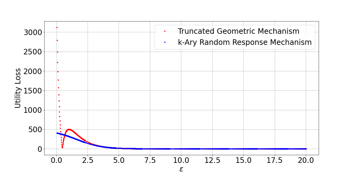
(a) Complete results for $0.0<\varepsilon\leq 20.0$.

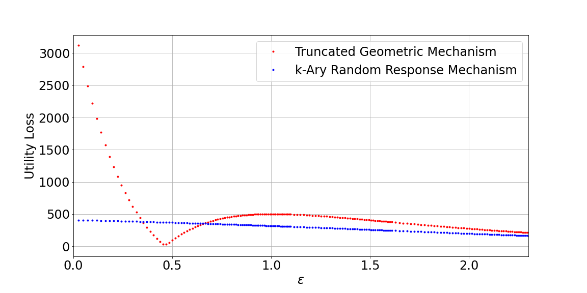
(b) Partial results for $0.0<\varepsilon\leq 2.3$.

Figure 4. Example of instability in the public domain

Our next example is taken from the public domain, an investigation of the relationship between utility and privacy in the general scenario of Fig. LABEL:fig:post-processing-pipelineX. We used a publicly available dataset released by ProPublica,  which contains two years’ worth of data from the COMPAS tool,  to produce the graphs of Fig. 4.

The data were pre-processed for consistency, resulting in a dataset with 11,710 unique records.  Each individual record had its “custody status” attribute converted to a number and then perturbed by the truncated geometric mechanism ${\mathit{G}D}_{\varepsilon}$ (Def. 5) of differential privacy.  The collection of perturbed data was then shuffled, so the link between each data subject and their randomised value was lost. The counting query “ Count the number of individuals with ‘custody status’ value equal to ‘pretrial defendant’ ” was then performed as a post-processing of the resulting collection of perturbed and shuffled values. Consider that a data analyst seeing the result of this query has as prior knowledge the original values for all individuals’ “custody status” except for a single individual considered to be the target. The analyst assumes, also as prior knowledge, that this individual’s unknown value has the same distribution derived from the frequency of the known values, and that her goal is to find out this individual’s value. Her chosen utility measure is the posterior Bayes’ risk (Eqn. (3)) of the counting query on the real data given the reported value for that same query on the perturbed data.

Fig. 4 presents the results of the experiment in the above scenario for various values of $\varepsilon$; and we can see from those results that this combination –the ${\mathit{G}D}$ perturbation and subsequent counting– is unstable in the exact sense defined in the main body of this paper: it is not order-preserving in expected loss ($y$ axis) as a function of the DP parameter $\varepsilon$ ($x$ axis). More precisely, as $\varepsilon$ grows, the utility loss of the geometric mechanism decreases and then increases again, as depicted in Fig. 4(a), and in more detail in Fig. 4(b). For the sake of comparison, we also present the results for an experiment in which the $N$-way random response of Sec. 6.1 is applied locally instead of the truncated geometric mechanism ${\mathit{G}D}_{\varepsilon}$: as predicted by Thm. 1, this scenario is stable and utility is monotonic wrt. privacy.

In our experiments we originally regarded this as an anomaly whose explanation could have been either a bug in our analysis code, or a consequence of rounding errors in the arithmetic. After investigating these possibilities, and finding that neither seemed to be the cause, we sought a concrete way to confirm that Fig. 4 was indeed the correct representation of the actual behaviour of the scenario. In order to do that we created a minimal counterexample for this scenario, using exact arithmetic, that accounts theoretically for the unstable behaviour we observed.

10. Discussion

The literature on formal proofs for privacy is very broad, with some techniques applicable to actual implementations in code (DBLP:conf/aplas/McIverM19, ; DBLP:conf/csfw/BartheGAHKS14, ; Barthe:16, ). Less attention has been paid however to utility, and in particular to its fine-grained behaviour in relation to $\varepsilon$. The application of refinement has been found to be useful for studies of optimality (DBLP:conf/csfw/FernandesMPD22, ) in the sense of Ghosh et al. (Ghosh2009, ). Here we found that the notion of stability appears to be another useful property indicating that complex mechanisms are behaving well from the point of view of an analyst. This is because the presence of unstable behaviour means that the post-processing part of the mechanism is actually losing information that is useful to the analyst: when there is no post-processing at all there is never any unstable behaviour.  (That means the post-processing has incorrectly collapsed columns of the perturbing channel.) In particular, instability could indicate bugs in the post-processing algorithm, and so testing for it could be used as a useful debugging tool, complementing analysis of privacy (Ding_2018, ).

Further, any fine-grained analysis must be tractable: what we have shown here is that the Kronecker product and its algebra enables precise modelling of Bayesian properties and simple algebraic-style proofs — from which we can draw strong and very general conclusions about utility, as well as simplifying proofs that verify privacy. The Kronecker product has also been used in modelling complex networks and data (10.5555/1756006.1756039, ; 10.1214/22-SS139, ) and we believe its further development for understanding privacy and utility will be similarly fruitful.

Finally, the assumption that $\varepsilon$ controls the trade-off between privacy and utility in $\varepsilon$-DP is widespread, and often openly endorsed by seasoned researchers and members of governmental statistical agencies. For example, Ghandi and Jayanti remark: “If the privacy loss parameter [in $\varepsilon$-DP] is set to favor utility, the privacy benefits are lowered (less “noise” is injected into the system); if the privacy loss parameter is set to favor heavy privacy, the accuracy and utility of the dataset are lowered (more “noise” is injected into the system)” (GA2020, , p.10). Our concept of stability is, to the best of our knowledge, the first rigorous formalization of this assumption, and we were able to identify situations in which it does hold, and does not hold. We believe this is a relevant contribution to various privacy practitioners and policy-makers that design and evaluate ever more complex private systems, and that it may allow for the construction of simultaneously more private and useful pipelines. As some of our results suggest, a possible cost of stability is that some DP-mechanisms may not be compatible with some post-processing algorithms. However, we do not yet know whether, under a different encoding of the privacy pipeline, stability could be in principle recovered. This question is left as future work.

11. Related work

Differential privacy was first proposed by Dwork et al. in 2006 (Dwork2006, ) and presents closure for privacy loss under post-processing (Dwork2013, ). The local model was first formalized by Kasiviswanathan et al. in 2011 (Kasiviswanathan2011, ) as a generalization of randomised response, first proposed by Warner in 1965 (Warner1965, ) and motivated by scenarios in which respondents do not trust the data curator.

Motivated by the reconstruction of statistical datasets via sequential queries proposed by Dinur and Nissim in 2003 (Dinur2003, ), the United States Census Bureau (USCB) started the adoption of differential privacy in 2008 (Machanavajjhala2008, ) and developed the TopDown algorithm for the 2020 Census (Abowd2018, ; Abowd2022, ). The final version of the TopDown algorithm was implemented using the discrete Gaussian mechanism (Canonne2020, ), but previous demonstration data products based on data from the 2010 Census used the geometric mechanism (Ghosh2009, ) instead. The choice of the discrete Gaussian over the geometric mechanism was the result of empirical accuracy tests of the TopDown algorithm using each mechanism with comparable privacy-loss budgets (Abowd2022, ). The budget allocation for the geometric mechanism under pure differential privacy (i.e. $\delta=0$) was determined using $\varepsilon$-allocation for a total of $\varepsilon=6$ (Abowd2022, ), while for the discrete Gaussian mechanism under zero-Concentrated Differential Privacy (zCDP) it was determined using $\rho$-allocation, with equivalent $\varepsilon$-allocation ranging from $\varepsilon=4.36$ to $\varepsilon=19.61$ (the production value (UnitedStatesCensusBureau2021, )).

The choice of values for the parameter $\varepsilon$ has been discussed since the inception of differential privacy and is usually regarded as a “social question” (Dwork2008, ), with values of $\varepsilon$ often ranging from $0.01$ to $10$ but without solid grounds for those choices (Hsu2014, ). One of the main challenges concerns the impact of the introduced noise, whose original goal is to protect respondents’ privacy, on data accuracy and its usefulness to data analysts. This notion of an inverse relationship, or a trade-off, between privacy preservation and accuracy has been widely reported on the literature, e.g.: Dwork and Roth state in (Dwork2013, ) that “A smaller $\varepsilon$ will yield better privacy (and less accurate responses)”, Hsu et al. state in (Hsu2014, ) that “$\varepsilon$ is a knob that trades off between privacy and utility”, and a report commissioned by the USCB (JASON2020, ) state that “The trade-off between confidentiality and statistical accuracy is reflected in the choice of the DP privacy-loss parameter. A low value increases the level of injected noise (and thus also confidentiality) but degrades statistical calculations”.

Data-release pipelines such as the one in Fig. LABEL:fig:post-processing-pipelineX have been reported, e.g.  by the USCB for its TopDown algorithm (Abowd2021, ; CommitteeOnNationalStatistics2020, ). Their pipeline starts with the Census microdata from which “noisy measurements” are made to create histograms by applying differential privacy. A post-processing step follows to satisfy invariants and constraints and to generate privacy-protected microdata, which is then used to create the USCB products (CommitteeOnNationalStatistics2020, ). In particular, this pipeline resembles that for the noisy $\mathit{A}rgMax$ from Sec. 8.1. According to the USCB, from the two primary sources of error within the TopDown algorithm, i.e. “measurement error” from adding noise into histograms cells counts and “post-processing error”, the latter is “much larger” (CommitteeOnNationalStatistics2020, ).

Quantitative Information Flow was pioneered by Clark, Hunt, and Malacaria (Clark:01:ENTCS, ), followed by a growing community, e.g. (Malacaria:07:POPL, ; Chatzikokolakis:08, ; Smith2009, ), and its principles have been organized in (Alvim20:Book, ). Moreover, the Haskell-based Kuifje programming language (Gibbons2020, ; Bognar2019, ) is able to interpret exactly the code given in the algorithms provided here.

12. Conclusions

We have presented a novel formal analysis technique for investigating the fine-grained behaviour of utility in privacy-preserving pipelines for large datasets. The analysis is based on Kronecker products and the theory of quantitative information flow, including its refinement order and the soundess/completeness property. Using this framework we are able to define the property of stability which seems to be a useful feature for simplifying the goal of finding the smallest privacy parameter to achieve a desired level of utility. Further, we are able to formally verify that any pipeline design using random response and counting will certainly be stable. Moreover we have also been able to explain anomalous behaviour observed in other privacy-preserving mechanisms that use geometric perturbers and counting. In the future a technique that produces small counterexamples might prove useful as a debugging tool.

One of our most compelling contributions is the use of Kronecker products applied to large data analyses, offering the prospect of tractable formal analysis for the verification of fine-grained statistical properties, perhaps applied to the verification of implementations of privacy-preserving libraries. In the future we would like to further develop the Kronecker method to complement the proof of privacy and utility in complex privacy pipelines.

Acknowledgments

Mário S. Alvim and Gabriel H.  Nunes were partially supported by CNPq, CAPES, and FAPEMIG. The research was partially funded by the European Research Council (ERC) project Hypatia, grant agreement № 835294.

Appendices

Appendix A Proofs for Sec. 5.3

Lemma 1.

(used to prove ($\hskip 1.00006pt\dagger$) in Lem. 3) Let $C$ be a $2{\times}2$ stochastic matrix (i.e. a channel) and $Y$ a tally as defined above. Then we have

(18) $$Y{\,{\cdot}\,}^{-1}Y\,{\cdot}\,{C}^{\otimes N}\,{\cdot}\,Y\quad=\quad{C}^{\otimes N}\,{\cdot}\,Y\makebox[0.0pt][l]{\quad\mbox{.}}$$

Proof.

Observe first that $Y_{s,k}=Y_{\sigma(s),k}$ for all permutations $\sigma$ of the indices of tuple $s$ in $\texttt{Bool}^{N}$. Further, since $Y$ is deterministic, there is exactly one value of $k$ for which that element of $Y$ is $1$. From this, we can define an equivalence relation $(\sim)$ on $N$-tuples $s,s^{\prime}$ in $\texttt{Bool}^{N}$, namely

$$s\sim s^{\prime}\qquad{\rm iff}\qquad Y_{s,-}=Y_{s^{\prime},-}\makebox[0.0pt][l]{\quad\mbox{.}}$$

Observe that each equivalence class is generated by all permutations of any element from the class: in effect two tuples are equivalent just when they yield the same $Y$-count.

For example if $s=(\texttt{true},\texttt{false},\texttt{true})$ then it would have $Y$-count of $2$, so that $Y_{s,2}=1$ and $Y_{s,k}=0$ for $k\neq 2$.

As a post-processor following ${C}^{\otimes N}$, the tally $Y$ merges all columns according to their equivalence classes.

As a pre-processor for ${C}^{\otimes N}\,{\cdot}\,Y$, any fixed left-inverse ${}^{-1}Y$ of the tally removes all but one of the rows corresponding to each equivalence class of tuple — and then the following tally $Y$ replaces the removed rows with the remaining row in the equivalence class.

The above taken together means that (15) holds if and only if $~{}Y_{s,-}=({C}^{\otimes N}\,{\cdot}\,Y)_{\sigma(s),-}~{}$ for all permutations $\sigma$. And we can show that by direct calculation, since $C$ is so specific: let it be the matrix

$$\left(\begin{array}[]{cc}a&b\\ c&d\end{array}\right)\makebox[0.0pt][l]{\quad\mbox{,}}$$

and let $Y$ be such that $Y_{s,k}=1$, i.e. that tuple $s$ contains exactly $k$ occurrences of true. Then, from a direct calculation we have that $~{}({C}^{\otimes N}\,{\cdot}\,Y)_{s,m}~{}$ is the sum of the probabilities that the output tuple $s^{\prime}$ from ${C}^{\otimes N}$, i.e. the tuple passed from $C$ to $Y$, has $m$ occurrences of true. The overall probability distribution of the output tuple is determined by executing $k$ (independent) random choices according to the distribution given by the first row of $C$, and $N{-}k$ (independent) random choices according to the distribution given by the second row of $C$. And to find that distribution we need to sum for each $m$ the probabilities of all the output sequences that have tally $m$.

Using probability-generating functions, that is equal to the $m$’th coefficient of $t^{m}$ in the polynomial $(at+b)^{k}(ct+d)^{N-k}$. Since this is not affected by permutations of $s$, the result follows. ∎

Appendix B Stability proof for a Geometric perturber and counting outliers

Recall from Sec. 7 the scenario where the analyst receives perturbed data according to a geometric definition with three possible outputs. Here she wants to count outliers of either kind thus uses an aggregator as in Def. 5.2:

$$L_{y,t}\quad:=\quad~{}~{}[y\in\{0,2\}]~{}~{}~{}~{}\textit{\quad and\quad}~{}~{}~{}~{}\quad L_{y,f}\quad:=\quad~{}~{}[y\not\in\{0,2\}]~{}.$$

In this case, it turns out that $L$ and ${L}^{\otimes N}$ satisfy the conditions for Thm. 1 wrt. the witness for refinement for $G_{3}\sqsubseteq G_{2}$, thus we do have that ${G_{3}}^{\otimes N}\,{\cdot}\,({L}^{\otimes N}\,{\cdot}\,Y)\sqsubseteq{G_{2}}^{\otimes N}\,{\cdot}\,({L}^{\otimes N}\,{\cdot}\,Y)$. The details are as follows:

1. The witness $W$ for refinement $G_{3}\sqsubseteq G_{2}$ is given by $(G_{3})^{-1}\,{\cdot}\,G_{2}$ which is:

   $$\begin{bmatrix}5/6&1/12&1/12\\ 7/30&8/15&7/30\\ 1/12&1/12&5/6\end{bmatrix}$$

2. The full matrix form of $L$ above is:

   $$\begin{bmatrix}1&0\\ 0&1\\ 1&0\end{bmatrix}~{},$$

3. and its left inverse ${}^{-1}L$ is:

   $$\begin{bmatrix}1&0&0\\ 0&1&0\end{bmatrix}~{}$$

4. We can now readily confirm that $L\,{\cdot}\,^{-1}L\,{\cdot}\,W\,{\cdot}\,L=W\,{\cdot}\,L$ , as required.

Appendix C More details for $\mathit{A}rgMax$

Kronecker products satisfy the pleasant additive property for privacy, which can be conveniently expressed using $d$-privacy (DBLP:phd/hal/Fernandes21, ). Let $d$ be some metric over the inputs of a channel $C$. This means that for any inputs $x,x^{\prime}$, and ouput $y$, we must have that $C_{x,y}\leq e^{d(x,x^{\prime})}{\times}C_{x^{\prime},y}$ Then we can say:

If $C$ is $d$-private, then ${C}^{\otimes N}$ is $d_{M}$-private ,

where $d_{M}$ is the “Manhattan” distance on the $N$-sequence inputs to ${C}^{\otimes N}$, that is $d_{M}(v,v^{\prime})=\sum_{0{\leq}i{<}N}d(v_{i},v_{i}^{\prime})$.

We can apply this to the noisy $\mathit{A}rgMax$ by observing that ${\mathit{G}D}_{\varepsilon}$ is $\varepsilon{\times}{|\cdot|}$-private, where the metric $|\cdot|$ is simply the difference $|x-x^{\prime}|$ for integer inputs $x,x^{\prime}$. Thus ${{\mathit{G}D}_{\varepsilon}}^{\otimes N}$ is $\varepsilon{\times}|\cdot|_{M}$-private.

Post-processing by $\mathit{A}rgMax$ certainly preserves this privacy property, by DPI, thus noisy $\mathit{A}rgMax$  is also $\varepsilon{\times}|\cdot|_{M}$-private. But this reduces to the normal meaning of $\varepsilon$-privacy because we only need to look at two adjacent histograms, namely inputs $h,h^{\prime}$ that differ in exactly one bar (or index), and only by one value, viz. there is some $j$ such that $|h_{j}-h^{\prime}_{j}|=1$, and for all other histogram bars $i\neq j$ we have that $h_{i}=h^{\prime}_{i}$. In this case we have that $\varepsilon{\times}|h-h^{\prime}|_{M}=\sum_{0{\leq}i{<}N}\varepsilon{\times}|h_{i}-h^{\prime}_{i}|=\varepsilon$. The result now follows.

Appendix D Examples of instability

As we discussed in the main body of this paper, “instability” is a situation in which privacy is increased (resp. decreased) in part of a data-release pipeline (and, as a consequence of differential privacy’s property of resistance to post-processing, in the overall pipeline as well), and yet the utility of the whole pipeline also increases (resp. decreases). The phenomenon is perhaps surprising because privacy practitioners normally make decisions under the assumption that privacy and utility go in opposite directions.

In this section we provide two examples of instability. The first is derived from a common data-release pipeline applied to a real dataset, and it illustrates how the phenomenon can indeed occur in practical scenarios (Sec. 9.2). The second is a minimal example of that same phenomenon, but now one that can be checked step-by-step, therefore certifying that the instability we discovered did not arise from coding– or rounding-errors.

D.1. Instability that can be checked manually

The instability from Sec. 9.2 above was calculated by the authors running their own code. (It was the database itself that was public.) We emphasize that the results are not limited to a few runs of the mechanism, but it is an exact computation of the expected behavior of the mechanism (in terms of $\varepsilon$’s and $U$’s) with respect to all coin tosses of the mechanism itself and the uncertainty of the data analyst’s prior distribution on the input to the mechanism.

In order to verify that the phenomenon is not a consequence of incorrect code or rounding errors, we constructed a small scenario of instability that can be checked by hand and employs only exact, rational arithmetic. In this example we have that:

1. There are only 4 individuals, each with a sensitive attribute taking an integer value between 0 and 6.

2. The data analyst knows the real values of the first 3 individuals to be $(0,1,1)$, and has a uniform prior on the value of the 4^th individual, that is, $\nicefrac{{1}}{{7}}$ for each of the values from 0 to 6.

3. The data analyst runs the the query “ How many individuals have sensitive value 0 in the dataset? ”, and her loss function is based on the absolute difference between the real value $x$ for the 4^th individual and the value $w$ she guesses for it, that is we define $\ell$ as

   (19) $$\ell(x,w)\quad=\quad 1000*|w-x|~{}\makebox[0.0pt][l]{\quad\mbox{,}}$$

   which can be represented in matrix form (with guesses $w$ as rows and real values $x$ as columns) as

   $$\begin{array}[]{c|ccccccc}&0&1&2&3&4&5&6\\ \hline\cr 0&0&1000&2000&3000&4000&5000&6000\\ 1&1000&0&1000&2000&3000&4000&5000\\ 2&2000&1000&0&1000&2000&3000&4000\\ 3&3000&2000&1000&0&1000&2000&3000\\ 4&4000&3000&2000&1000&0&1000&2000\\ 5&5000&4000&3000&2000&1000&0&1000\\ 6&6000&5000&4000&3000&2000&1000&0\\ \end{array}~{}.$$

4. The truncated geometric mechanism ${\mathit{G}D}_{\varepsilon}$ realizing $\varepsilon$-DP  is then used for perturbation of each individual record, where in this first case $\varepsilon$ is $~{}\ln 3.50$. If we represent ${\mathit{G}D}_{\varepsilon}$’s effect as a matrix whose rows contain possible actual values for each individual, and whose columns contain possible randomized values, we get

   (28) $$\begin{array}[]{c|ccccccc}&0&1&2&3&4&5&6\\ \hline\cr 0&\nicefrac{{7}}{{9}}&\nicefrac{{10}}{{63}}&\nicefrac{{20}}{{441}}&\nicefrac{{40}}{{3087}}&\nicefrac{{80}}{{21609}}&\nicefrac{{160}}{{151263}}&\nicefrac{{64}}{{151263}}\\ 1&\nicefrac{{2}}{{9}}&\nicefrac{{5}}{{9}}&\nicefrac{{10}}{{63}}&\nicefrac{{20}}{{441}}&\nicefrac{{40}}{{3087}}&\nicefrac{{80}}{{21609}}&\nicefrac{{32}}{{21609}}\\ 2&\nicefrac{{4}}{{63}}&\nicefrac{{10}}{{63}}&\nicefrac{{5}}{{9}}&\nicefrac{{10}}{{63}}&\nicefrac{{20}}{{441}}&\nicefrac{{40}}{{3087}}&\nicefrac{{16}}{{3087}}\\ 3&\nicefrac{{8}}{{441}}&\nicefrac{{20}}{{441}}&\nicefrac{{10}}{{63}}&\nicefrac{{5}}{{9}}&\nicefrac{{10}}{{63}}&\nicefrac{{20}}{{441}}&\nicefrac{{8}}{{441}}\\ 4&\nicefrac{{16}}{{3087}}&\nicefrac{{40}}{{3087}}&\nicefrac{{20}}{{441}}&\nicefrac{{10}}{{63}}&\nicefrac{{5}}{{9}}&\nicefrac{{10}}{{63}}&\nicefrac{{4}}{{63}}\\ 5&\nicefrac{{32}}{{21609}}&\nicefrac{{80}}{{21609}}&\nicefrac{{40}}{{3087}}&\nicefrac{{20}}{{441}}&\nicefrac{{10}}{{63}}&\nicefrac{{5}}{{9}}&\nicefrac{{2}}{{9}}\\ 6&\nicefrac{{64}}{{151263}}&\nicefrac{{160}}{{151263}}&\nicefrac{{80}}{{21609}}&\nicefrac{{40}}{{3087}}&\nicefrac{{20}}{{441}}&\nicefrac{{10}}{{63}}&\nicefrac{{7}}{{9}}\\ \end{array}~{}.$$

   Now, if each individual randomises their own value with the matrix above, and then all perturbed values are shuffled to break the link between each data subject and their perturbed value, we obtain the following matrix that maps the value of the 4^th individual (rows) to the final count of the query (columns), given that the actual values for the first three individuals are known to be (0,1,1):

   (37) $$\begin{array}[]{c|ccccc}&0&1&2&3&4\\ \hline\cr 0&\nicefrac{{196}}{{6561}}&\nicefrac{{1484}}{{6561}}&\nicefrac{{1067}}{{2187}}&\nicefrac{{1484}}{{6561}}&\nicefrac{{196}}{{6561}}\\ 1&\nicefrac{{686}}{{6561}}&\nicefrac{{2989}}{{6561}}&\nicefrac{{742}}{{2187}}&\nicefrac{{604}}{{6561}}&\nicefrac{{56}}{{6561}}\\ 2&\nicefrac{{826}}{{6561}}&\nicefrac{{3419}}{{6561}}&\nicefrac{{4544}}{{15309}}&\nicefrac{{2468}}{{45927}}&\nicefrac{{16}}{{6561}}\\ 3&\nicefrac{{866}}{{6561}}&\nicefrac{{24793}}{{45927}}&\nicefrac{{30508}}{{107163}}&\nicefrac{{13756}}{{321489}}&\nicefrac{{32}}{{45927}}\\ 4&\nicefrac{{6142}}{{45927}}&\nicefrac{{175271}}{{321489}}&\nicefrac{{210956}}{{750141}}&\nicefrac{{89252}}{{2250423}}&\nicefrac{{64}}{{321489}}\\ 5&\nicefrac{{43154}}{{321489}}&\nicefrac{{1230337}}{{2250423}}&\nicefrac{{1471492}}{{5250987}}&\nicefrac{{610684}}{{15752961}}&\nicefrac{{128}}{{2250423}}\\ 6&\nicefrac{{302398}}{{2250423}}&\nicefrac{{8619239}}{{15752961}}&\nicefrac{{10290044}}{{36756909}}&\nicefrac{{4246628}}{{110270727}}&\nicefrac{{256}}{{15752961}}\\ \end{array}~{}.$$

   Under a uniform prior, that leads to an expected utility loss of $\nicefrac{{1276949536000}}{{771895089}}\approx 1654.3045$.

5. If now, in the second case, $\varepsilon$ is set to the slightly higher (i.e. less private) value of $\ln 3.51$, we obtain instead the following perturbation matrix representing each individual’s randomization via ${\mathit{G}D}_{\varepsilon}$:

   (56) $$\begin{array}[]{c}\begin{array}[]{c|cccc}&0&1&2&3\\ \hline\cr 0&\nicefrac{{351}}{{451}}&\nicefrac{{25100}}{{158301}}&\nicefrac{{2510000}}{{55563651}}&\nicefrac{{251000000}}{{19502841501}}\\ 1&\nicefrac{{100}}{{451}}&\nicefrac{{251}}{{451}}&\nicefrac{{25100}}{{158301}}&\nicefrac{{2510000}}{{55563651}}\\ 2&\nicefrac{{10000}}{{158301}}&\nicefrac{{25100}}{{158301}}&\nicefrac{{251}}{{451}}&\nicefrac{{25100}}{{158301}}\\ 3&\nicefrac{{1000000}}{{55563651}}&\nicefrac{{2510000}}{{55563651}}&\nicefrac{{25100}}{{158301}}&\nicefrac{{251}}{{451}}\\ 4&\nicefrac{{100000000}}{{19502841501}}&\nicefrac{{251000000}}{{19502841501}}&\nicefrac{{2510000}}{{55563651}}&\nicefrac{{25100}}{{158301}}\\ 5&\nicefrac{{10000000000}}{{6845497366851}}&\nicefrac{{25100000000}}{{6845497366851}}&\nicefrac{{251000000}}{{19502841501}}&\nicefrac{{2510000}}{{55563651}}\\ 6&\nicefrac{{1000000000000}}{{2402769575764701}}&\nicefrac{{2510000000000}}{{2402769575764701}}&\nicefrac{{25100000000}}{{6845497366851}}&\nicefrac{{251000000}}{{19502841501}}\end{array}\\ \begin{array}[]{c|ccc}&4&5&6\\ \hline\cr 0&\nicefrac{{25100000000}}{{6845497366851}}&\nicefrac{{2510000000000}}{{2402769575764701}}&\nicefrac{{1000000000000}}{{2402769575764701}}\\ 1&\nicefrac{{251000000}}{{19502841501}}&\nicefrac{{25100000000}}{{6845497366851}}&\nicefrac{{10000000000}}{{6845497366851}}\\ 2&\nicefrac{{2510000}}{{55563651}}&\nicefrac{{251000000}}{{19502841501}}&\nicefrac{{100000000}}{{19502841501}}\\ 3&\nicefrac{{25100}}{{158301}}&\nicefrac{{2510000}}{{55563651}}&\nicefrac{{1000000}}{{55563651}}\\ 4&\nicefrac{{251}}{{451}}&\nicefrac{{25100}}{{158301}}&\nicefrac{{10000}}{{158301}}\\ 5&\nicefrac{{25100}}{{158301}}&\nicefrac{{251}}{{451}}&\nicefrac{{100}}{{451}}\\ 6&\nicefrac{{2510000}}{{55563651}}&\nicefrac{{25100}}{{158301}}&\nicefrac{{351}}{{451}}\\ \end{array}\end{array}~{}.$$

   This leads instead to the following mapping from the value of the 4^th individual (rows) to the final count of the query (columns), again given that perturbed values were shuffled and that the actual values for the first three individuals are known to be (0,1,1):

   (75) $$\begin{array}[]{c}\begin{array}[]{c|ccccc}&0&1&2\\ \hline\cr 0&\nicefrac{{1232010000}}{{41371966801}}&\nicefrac{{9350710200}}{{41371966801}}&\nicefrac{{20206526401}}{{41371966801}}\\ 1&\nicefrac{{4324355100}}{{41371966801}}&\nicefrac{{18874516401}}{{41371966801}}&\nicefrac{{14026065300}}{{41371966801}}\\ 2&\nicefrac{{5205365100}}{{41371966801}}&\nicefrac{{21587851501}}{{41371966801}}&\nicefrac{{4305102810200}}{{14521560347151}}\\ 3&\nicefrac{{5456365100}}{{41371966801}}&\nicefrac{{7848669386851}}{{14521560347151}}&\nicefrac{{1449286475370200}}{{5097067681850001}}\\ 4&\nicefrac{{1940284150100}}{{14521560347151}}&\nicefrac{{2782016305784701}}{{5097067681850001}}&\nicefrac{{502519091753940200}}{{1789070756329350351}}\\ 5&\nicefrac{{683549736685100}}{{5097067681850001}}&\nicefrac{{979201058430430051}}{{1789070756329350351}}&\nicefrac{{175766155095533010200}}{{627963835471601973201}}\\ 6&\nicefrac{{240176957576470100}}{{1789070756329350351}}&\nicefrac{{343970905019080947901}}{{627963835471601973201}}&\nicefrac{{61632115827522086580200}}{{220415306250532292593551}}\end{array}\\ \begin{array}[]{c|cc}&3&4\\ \hline\cr 0&\nicefrac{{9350710200}}{{41371966801}}&\nicefrac{{1232010000}}{{41371966801}}\\ 1&\nicefrac{{3796030000}}{{41371966801}}&\nicefrac{{351000000}}{{41371966801}}\\ 2&\nicefrac{{776938510000}}{{14521560347151}}&\nicefrac{{100000000}}{{41371966801}}\\ 3&\nicefrac{{217158615010000}}{{5097067681850001}}&\nicefrac{{10000000000}}{{14521560347151}}\\ 4&\nicefrac{{70667993668510000}}{{1789070756329350351}}&\nicefrac{{1000000000000}}{{5097067681850001}}\\ 5&\nicefrac{{24248997757647010000}}{{627963835471601973201}}&\nicefrac{{100000000000000}}{{1789070756329350351}}\\ 6&\nicefrac{{8455851410934100510000}}{{220415306250532292593551}}&\nicefrac{{10000000000000000}}{{627963835471601973201}}\end{array}\end{array}~{}.$$

   This counting query (75) above, under a uniform prior, has therefore not led to a utility gain over (37), wrt. loss function (19). This happened even though the $\varepsilon$-DP of the ${\mathit{G}D}$-perturber increased between (28) and (56), making the overall pipeline less private. Instead it led to a greater loss (that is, smaller utility) of $\nicefrac{{2552438666271995640492212000}}{{1542907143753726048154857}}\approx 1654.3047$ (i.e. more than the loss of $1654.3045$ just above). This is exactly the phenomenon of instability.

D.2. Demonstrating instability without a counter example

The Sec. 9 illustrated by experiment the apparent stability of noisy $\mathit{A}rgMax$ in three scenarios. Is it still possible that there might be a prior distribution $\pi$ and a parameter $\varepsilon$ for which ${\mathit{G}D}_{\varepsilon}$ followed by $\mathit{A}rgMax$ is unstable, and can we we show that to be so without finding the actual $\pi$ and $\varepsilon$? What we want (for instability) is two geometric perturbers such that

(76) $${\mathit{G}D}_{\varepsilon}\sqsubseteq{\mathit{G}D}_{\varepsilon^{\prime}}\qquad{\rm and~{}yet}\qquad{\mathit{G}D}_{\varepsilon}\,{\cdot}\,\mathit{A}rgMax~{}\not\sqsubseteq~{}{\mathit{G}D}_{\varepsilon^{\prime}}\,{\cdot}\,\mathit{A}rgMax\makebox[0.0pt][l]{\quad\mbox{,}}$$

but in its Kroneckered version of course. The lhs is equivalent to $\varepsilon^{\prime}{\leq}\varepsilon$ because ${\mathit{G}D}$ is a family. Can we get the $(\not\sqsubseteq)$ on the rhs from Thm. 1?

A first step we can take is to note that ${\mathit{G}D}_{\varepsilon}\sqsubseteq{\mathit{G}D}_{\varepsilon^{\prime}}$ means that ${\mathit{G}D}_{\varepsilon}\,{\cdot}\,W={\mathit{G}D}_{\varepsilon^{\prime}}$ for some witness $W$, and so the rhs of (76) requires

(77) $${\mathit{G}D}_{\varepsilon}\,{\cdot}\,\mathit{A}rgMax\quad\not\sqsubseteq\quad{\mathit{G}D}_{\varepsilon}\,{\cdot}\,W\,{\cdot}\,\mathit{A}rgMax$$

for that $W$. Although it is tempting now to use the only if of Thm. 1 with a $W$ satisfying

$$\mathit{A}rgMax\,{\cdot}\,^{-1}\mathit{A}rgMax\,{\cdot}\,W\,{\cdot}\,\mathit{A}rgMax\quad\neq\quad W\,{\cdot}\,\mathit{A}rgMax$$

to get $\mathit{A}rgMax\not\sqsubseteq W\,{\cdot}\,\mathit{A}rgMax$, then inferring our target (77) by applying $({\mathit{G}D}_{\varepsilon}\,{\cdot}\,)$ to both sides… that’s not valid. You cannot conclude $f(x)\,{\not\sqsubseteq}\,f(x^{\prime})$ from $x\,{\not\sqsubseteq}\,x^{\prime}$.

Instead, we “start further back” — and it seems to depend on ${\mathit{G}D}_{\varepsilon}$’s having an inverse. We assume ${\mathit{G}D}_{\varepsilon}\sqsubseteq{\mathit{G}D}_{\varepsilon^{\prime}}$, the lhs of (76), and then reason as follows (without Kronecker, because it can be added later ), writing $\mathit{A}rgMax$ as $P$ for brevity:

	$\begin{array}[t]{@{}ll}{}\\ P\,{\cdot}\,^{-1}P\,{\cdot}\,{\mathit{G}D}_{\varepsilon}^{-1}\,{\cdot}\,{\mathit{G}D}_{\varepsilon^{\prime}}\,{\cdot}\,P\quad\neq\quad{\mathit{G}D}_{\varepsilon}^{-1}\,{\cdot}\,{\mathit{G}D}_{\varepsilon^{\prime}}\,{\cdot}\,P\end{array}$ “assumption $(\dagger)$”
hence	$\begin{array}[t]{@{}ll}{}\\ P\quad\not\sqsubseteq\quad{\mathit{G}D}_{\varepsilon}^{-1}\,{\cdot}\,{\mathit{G}D}_{\varepsilon^{\prime}}\,{\cdot}\,P\end{array}$ “Equation (12), “only if”, in Thm. 1, with $W$ as ${\mathit{G}D}_{\varepsilon}^{-1}\,{\cdot}\,{\mathit{G}D}_{\varepsilon^{\prime}}$”
iff	$\begin{array}[t]{@{}ll}{}\\ P\,{\cdot}\,V\quad\neq\quad{\mathit{G}D}_{\varepsilon}^{-1}\,{\cdot}\,{\mathit{G}D}_{\varepsilon^{\prime}}\,{\cdot}\,P\end{array}$ “for all $V$, definition witness”
iff	$\begin{array}[t]{@{}ll}{}\\ {\mathit{G}D}_{\varepsilon}^{-1}\,{\cdot}\,{\mathit{G}D}_{\varepsilon}\,{\cdot}\,P\,{\cdot}\,V\quad\neq\quad{\mathit{G}D}_{\varepsilon}^{-1}\,{\cdot}\,{\mathit{G}D}_{\varepsilon^{\prime}}\,{\cdot}\,P\end{array}$ “identity on left”
hence	$\begin{array}[t]{@{}ll}{}\\ {\mathit{G}D}_{\varepsilon}\,{\cdot}\,P\,{\cdot}\,V\quad\neq\quad{\mathit{G}D}_{\varepsilon^{\prime}}\,{\cdot}\,P\end{array}$ “in general $f(x){\neq}f(x^{\prime})$ implies $x{\neq}x^{\prime}$”
hence	$\begin{array}[t]{@{}ll}{}\\ {\mathit{G}D}_{\varepsilon}\,{\cdot}\,P\quad\not\sqsubseteq\quad{\mathit{G}D}_{\varepsilon^{\prime}}\,{\cdot}\,P\makebox[0.0pt][l]{\quad\mbox{,}}\end{array}$ “using ‘for all $V$’ from above, Def. 3 of refinement and witness”

which is the rhs of (76) that we wanted. So if we can find an instance of the assumption $(\dagger)$, now written out in full as

$$\mathit{A}rgMax\,{\cdot}\,^{-1}\mathit{A}rgMax\,{\cdot}\,{\mathit{G}D}_{\varepsilon}^{-1}\,{\cdot}\,{\mathit{G}D}_{\varepsilon^{\prime}}\,{\cdot}\,\mathit{A}rgMax$$

$$\neq {\mathit{G}D}_{\varepsilon}^{-1}\,{\cdot}\,{\mathit{G}D}_{\varepsilon^{\prime}}\,{\cdot}\,\mathit{A}rgMax\makebox[0.0pt][l]{\quad\mbox{,}}$$

then we know from Thm. 4 that ${\mathit{G}D}_{\varepsilon},{\mathit{G}D}_{\varepsilon^{\prime}}$ and $\mathit{A}rgMax$ must together be unstable.

But what have we gained?

The assumption $(\dagger)$ is if anything more complex than the conclusion ${\mathit{G}D}_{\varepsilon}\,{\cdot}\,P\,\sqsubseteq\,{\mathit{G}D}_{\varepsilon^{\prime}}\,{\cdot}\,P$ we used it to reach. And in both cases we still have to search through ${\mathit{G}D}_{\varepsilon}$’s and ${\mathit{G}D}_{\varepsilon^{\prime}}$’s to find an instance of $(\dagger)$.

What we’ve gained is that showing an inequality $(\neq)$ is much easier –computationally– than showing a refinement-failure $(\not\sqsubseteq)$.

Appendix E Counter-example for sum queries

For the sum query counter-example, we had:

$$R_{2}=\begin{bmatrix}1/2&1/4&1/4\\ 1/4&1/2&1/4\\ 1/4&1/4&1/2\end{bmatrix}\qquad R_{3}=\begin{bmatrix}3/5&1/5&1/5\\ 1/5&3/5&1/5\\ 1/5&1/5&3/5\end{bmatrix}$$

And the sum query is defined:

001000001010000200100100100011001001200010200010021000102200001𝑆fragments 001000001010000200100100100011001001200010200010021000102200001\centering S=\begin{tabular}[]{c | c c c c c}&0&1&2&3&4\\ \hline\cr 00&1&0&0&0&0\\ 01&0&1&0&0&0\\ 02&0&0&1&0&0\\ 10&0&1&0&0&0\\ 11&0&0&1&0&0\\ 12&0&0&0&1&0\\ 20&0&0&1&0&0\\ 21&0&0&0&1&0\\ 22&0&0&0&0&1\end{tabular}\@add@centering

0123401234

Now, we want to show that $(R_{3}\otimes R_{3})\cdot S\not\sqsubseteq(R_{2}\otimes R_{2})\cdot S$. We can compute that $(R_{3}\otimes R_{3})\cdot S$ is:

0 1 2 3 4

00 0.36 0.24 0.28 0.08 0.04

01 0.12 0.4 0.28 0.16 0.04

02 0.12 0.16 0.44 0.16 0.12

10 0.12 0.4 0.28 0.16 0.04

11 0.04 0.24 0.44 0.24 0.04

12 0.04 0.16 0.28 0.4 0.12

20 0.12 0.16 0.44 0.16 0.12

21 0.04 0.16 0.28 0.4 0.12

22 0.04 0.08 0.28 0.24 0.36

and $(R_{2}\otimes R_{2})\cdot S$ is:

0 1 2 3 4

00 0.25 0.25 0.3125 0.125 0.0625

01 0.125 0.3125 0.3125 0.1875 0.0625

02 0.125 0.1875 0.375 0.1875 0.125

10 0.125 0.3125 0.3125 0.1875 0.0625

11 0.0625 0.25 0.375 0.25 0.0625

12 0.0625 0.1875 0.3125 0.3125 0.125

20 0.125 0.1875 0.375 0.1875 0.125

21 0.0625 0.1875 0.3125 0.3125 0.125

22 0.0625 0.125 0.3125 0.25 0.25

And we find the following counter-example loss function, in which columns correspond to actions and rows are $x$-labelled:

$$w_{1}$$

00 0.33525164 0.67014371 0.50295689 0.64597016 0.34089403

01 0.58508164 0.41408977 0.50010053 0.42214762 0.57379685

02 0.74867853 0.25036935 0.49712065 0.25036935 0.74867853

10 0.58508164 0.41408977 0.50010053 0.42214762 0.57379685

11 0. 1. 0.49521641 1. 0.

12 0.57379685 0.42214762 0.50010053 0.41408977 0.58508164

20 0.74867853 0.25036935 0.49712065 0.25036935 0.74867853

21 0.57379685 0.42214762 0.50010053 0.41408977 0.58508164

22 0.34089403 0.64597016 0.50295689 0.67014371 0.33525164

Appendix F Example: direct proof of stability for a special case

We illustrate the stability proof in Sec. 6.1 (random response and counting) by considering the special case in which there are $N{=}3$ participants and a single choice $k$ in $\mathcal{K}$ is tallied. (In Sec. 6.1 any $1{\leq}N$ of participants was allowed, and any subset of choices in $\mathcal{K}$ could be tallied.)

From Lem. 1 we recall that any single-respondent ${\mathit{R}R}_{\varepsilon}^{K}$ can be written $a\mathbb{I}+b\mathbb{U}$, where $\mathbb{I}$ is the identity matrix and $\mathbb{U}$ is a matrix all of whose elements are $\nicefrac{{1}}{{K}}$, both matrices being of size $K{\times}K$. In general however we’re interested in the $N{>}1$ -respondent case, with ${({\mathit{R}R}_{\varepsilon}^{K})}^{\otimes N}$ as the perturber: it would then be

(78) $${({\mathit{R}R}_{\varepsilon}^{K})}^{\otimes N}\quad=\quad\underbrace{(a\mathbb{I}+b\mathbb{U})\otimes\cdots\otimes(a\mathbb{I}+b\mathbb{U})}_{N}\makebox[0.0pt][l]{\quad\mbox{,}}\vspace{-2ex}$$

for some $a,b$.

Here we specialise to $N{=}3$, that is $3$ respondents, and we use the distribution laws for $\otimes$ to see that (78), that is  ${({\mathit{R}R}_{\varepsilon}^{K})}^{\otimes 3}_{(x_{1},x_{2},x_{3}),(y_{1},y_{2},y_{3})}$ becomes

	$\begin{array}[t]{@{}llll}\parbox{40.00006pt}{$a^{3}\,\times$}(\mathbb{I}\otimes\mathbb{I}\otimes\mathbb{I})_{(x_{1},x_{2},x_{3}),(y_{1},y_{2},y_{3})}\end{array}$
$+$	$\begin{array}[t]{@{}llll}\parbox{40.00006pt}{$a^{2}b\,\times$}(\mathbb{I}\otimes\mathbb{I}\otimes\mathbb{U})_{(x_{1},x_{2},x_{3}),(y_{1},y_{2},y_{3})}\end{array}$
$+$	$\begin{array}[t]{@{}llll}\parbox{40.00006pt}{$a^{2}b\,\times$}(\mathbb{I}\otimes\mathbb{U}\otimes\mathbb{I})_{(x_{1},x_{2},x_{3}),(y_{1},y_{2},y_{3})}\end{array}$
$+$	$\begin{array}[t]{@{}llll}\parbox{40.00006pt}{$a^{2}b\,\times$}(\mathbb{I}\otimes\mathbb{U}\otimes\mathbb{U})_{(x_{1},x_{2},x_{3}),(y_{1},y_{2},y_{3})}\end{array}$
$+$	$\begin{array}[t]{@{}llll}\parbox{40.00006pt}{$ab^{2}\,\times$}(\mathbb{U}\otimes\mathbb{I}\otimes\mathbb{I})_{(x_{1},x_{2},x_{3}),(y_{1},y_{2},y_{3})}\end{array}$
$+$	$\begin{array}[t]{@{}llll}\parbox{40.00006pt}{$ab^{2}\,\times$}(\mathbb{U}\otimes\mathbb{I}\otimes\mathbb{U})_{(x_{1},x_{2},x_{3}),(y_{1},y_{2},y_{3})}\end{array}$
$+$	$\begin{array}[t]{@{}llll}\parbox{40.00006pt}{$ab^{2}\,\times$}(\mathbb{U}\otimes\mathbb{U}\otimes\mathbb{I})_{(x_{1},x_{2},x_{3}),(y_{1},y_{2},y_{3})}\end{array}$
$+$	$\begin{array}[t]{@{}llll}\parbox{40.00006pt}{$b^{3}\,\times$}(\mathbb{U}\otimes\mathbb{U}\otimes\mathbb{U})_{(x_{1},x_{2},x_{3}),(y_{1},y_{2},y_{3})}\makebox[0.0pt][l]{\quad\mbox{,}}\end{array}$

where each $x_{n}$ (for $n{=}1,2,3$) is the choice in $\mathcal{K}$ made by respondent $n$, and each $y_{n}$ is the output to which the (individual) ${\mathit{R}R}_{\varepsilon}$ has perturbed the input choice $x_{n}$.

Evaluating each summand of the above (using Def. 3 of Kroneckering) gives us

(79) $$\begin{array}[t]{@{}llll}\parbox{50.00008pt}{$a^{3}\,\times$}[x_{1}{=}y_{1}\land x_{2}{=}y_{2}\land x_{3}{=}y_{3}]\end{array} + \begin{array}[t]{@{}llll}\parbox{50.00008pt}{$a^{2}b/K\,\times$}[x_{1}{=}y_{1}\land x_{2}{=}y_{2}]\end{array} + \begin{array}[t]{@{}llll}\parbox{50.00008pt}{$a^{2}b/K\,\times$}[x_{1}{=}y_{1}\land x_{3}{=}y_{3}]\end{array} + \begin{array}[t]{@{}llll}\parbox{50.00008pt}{$a^{2}b/K\,\times$}[x_{2}{=}y_{2}\land x_{3}{=}y_{3}]\end{array} + \begin{array}[t]{@{}llll}\parbox{50.00008pt}{$ab^{2}/K^{2}\,\times$}[x_{1}{=}y_{1}]\end{array} + \begin{array}[t]{@{}llll}\parbox{50.00008pt}{$ab^{2}/K^{2}\,\times$}[x_{2}{=}y_{2}]\end{array} + \begin{array}[t]{@{}llll}\parbox{50.00008pt}{$ab^{2}/K^{2}\,\times$}[x_{3}{=}y_{3}]\end{array} + \begin{array}[t]{@{}llll}\parbox{50.00008pt}{$b^{3}/K^{3}\,\times$}1\makebox[0.0pt][l]{\quad\mbox{,}}\end{array} [-]$$ where we use “Iverson brackets” to convert Booleans to 0,1.

Equation (79) is a single real number: it is the element of ${({\mathit{R}R}_{\varepsilon}^{K})}^{\otimes 3}$​​ indexed by row $(x_{1},x_{2},x_{3})$ and column $(y_{1},y_{2},y_{3})$. Now we want to look at the details of how a counting query $T$ interacts with a $W$ of the general form (79) above. We want to know in particular when the equality (11) from Thm. 1 holds, which we repeat here for our counting query $T$ specifically:

(80) $$T{\,{\cdot}\,}^{-1}T\,{\cdot}\,W\,{\cdot}\,T\quad=\quad W\,{\cdot}\,T\makebox[0.0pt][l]{\quad\mbox{.}}$$

Without loss of generality we assume that $\mathcal{K}$ is $\{1..K\}$, and we specialise to the case that $T$ is counting the single response $k{=}1$. (The Boolean aggregator $B$ from Def. 2 is more general because it can send any fixed subset of $\mathcal{K}$ to true.)

We begin with the leading $T{\,{\cdot}\,}^{-1}T$, i.e. on the left: its effect on an input 3-tuple $x$ is simply to move it to some (possibly other) 3-tuple $x^{\prime}$ in which the same number of 1’s occur.

Next we look at the effect of the trailing $T$, which is on both sides of the equation: it simply groups together $y$-output 3-tuples that have the same number of 1’s.

So to show that (80) holds, we must argue that if we change an input $x$ to another $x^{\prime}$ with the same number of 1’s, then for any number $0{\leq}t{\leq}N$ the sum (79) does not change when taken over all output-tuples with $t$ occurrences of 1. (In this case $N{=}3$, but the argument will be given in terms of $N$.)

We make that argument by changing $x$ into $x^{\prime}$ taking “one step at a time”. Remember that “1” is the value in $1..K$ that we are counting and assume –for the moment– that all 1’s in the input-tuple $x$ occur together at its beginning. That is, the input-tuple $x$ and the “one step away” $x^{\prime}$ are both of the form $(1,\ldots,1,k^{\prime},k^{\prime\prime}\ldots k^{\prime\prime\prime})$, where all the primed $k$’s are not 1 (but they are not necessarily all different).

Now suppose that in a single step we change some element $x_{n}$ of $x$ to $x^{\prime}_{n}$, i.e. we change the value at index $1{\leq}n{\leq}N$ that was supplied by Respondent $n$. We note first that neither $x_{n}$ nor $x^{\prime}_{n}$ can be 1, because otherwise that step would change the number of 1’s in $x$.

For each $y$ with a fixed count $0{\leq}t{\leq}N$ of 1’s there are now three possibilities for each of its elements $y_{n}$:

1. If $y_{n}{=}1$, then none of the summands in (79) will be affected, since neither $x_{n}$ nor $x^{\prime}_{n}$ is 1.

2. If $y_{n}\,{=}\,x_{n}$ but $y_{n}\,{\neq}\,x^{\prime}_{n}$, then for that $y$ some summands in (79) that include conjunct $x_{n}{=}y_{n}$ will change from 1 to 0, because the conjunct is no longer true.  But there is always another $y^{\prime}$ with the same count $t$ of 1’s, exactly identical to $y$ except that $y^{\prime}_{n}{=}x^{\prime}_{n}$, in which exactly the opposite change (i.e. from 0 to 1) will occur. Thus the overall sum –over all $y$’s with that count $t$ of 1’s– remains the same.

3. The third case, where $y_{n}{\neq}x_{n}$ but now $y_{n}{=}x^{\prime}_{n}$, is analogous to the second.

Finally, we can relax the restriction that all of the $x$-tuple’s occurrences of 1 must come first: that is because any target $x^{\prime}$ where the some 1’s do not come first can be reached from the $x$ with all its 1’s first simply by following the above step-by-step procedure until an intermediate $x^{\prime\prime}$ is reached that (still) has all its 1’s first and at the same time is a permutation of the final $x^{\prime}$ desired. It will have the same (79)-sum for any $y$ having $t$ instances of 1 as $x$ did, from the step-by-step argument above; but it will also have the same sum as the actual target $x^{\prime}$, because the subset of $\mathcal{Y}$ having exactly $t$ instances of 1 is permutation closed.

That completes our “proof by example” of (80) and hence (re-using material from Sec. 6.1) that multiple-participant random-response folowed by a counting query is stable.

References

- (1) A. Ghosh, T. Roughgarden, and M. Sundararajan, “Universally utility-maximizing privacy mechanisms,” in Proceedings of the 41st Annual ACM Symposium on Symposium on Theory of Computing - STOC ’09, (Bethesda, MD, USA), p. 351, ACM Press, 2009.
- (2) T. Asikis and E. Pournaras, “Optimization of privacy-utility trade-offs under informational self-determination,” Future Generation Computer Systems, vol. 109, pp. 488–499, 2020.
- (3) T. Li and N. Li, “On the tradeoff between privacy and utility in data publishing,” in Knowledge Discovery and Data Mining, 2009.
- (4) Q. Geng, W. Ding, R. Guo, and S. Kumar, “Tight analysis of privacy and utility tradeoff in approximate differential privacy,” in Proceedings of the Twenty Third International Conference on Artificial Intelligence and Statistics (S. Chiappa and R. Calandra, eds.), vol. 108 of Proceedings of Machine Learning Research, pp. 89–99, PMLR, 26–28 Aug 2020.
- (5) M. S. Alvim, N. Fernandes, A. McIver, and G. H. Nunes, “On privacy and accuracy in data releases (invited paper),” in 31st International Conference on Concurrency Theory, CONCUR 2020, September 1-4, 2020, Vienna, Austria (Virtual Conference) (I. Konnov and L. Kovács, eds.), vol. 171 of LIPIcs, pp. 1:1–1:18, Schloss Dagstuhl - Leibniz-Zentrum für Informatik, 2020.
- (6) C. Dwork and A. Roth, “The Algorithmic Foundations of Differential Privacy,” Foundations and Trends® in Theoretical Computer Science, vol. 9, no. 3-4, pp. 211–407, 2013.
- (7) Z. Ding, Y. Wang, G. Wang, D. Zhang, and D. Kifer, “Detecting violations of differential privacy,” in Proceedings of the 2018 ACM SIGSAC Conference on Computer and Communications Security, ACM, oct 2018.
- (8) U. Erlingsson, V. Pihur, and A. Korolova, “Rappor: Randomized aggregatable privacy-preserving ordinal response,” CCS ’14, (New York, NY, USA), p. 1054–1067, Association for Computing Machinery, 2014.
- (9) K. Nissim and H. Brenner, “Impossibility of differentially private universally optimal mechanisms,” in 2013 IEEE 54th Annual Symposium on Foundations of Computer Science, (Los Alamitos, CA, USA), pp. 71–80, IEEE Computer Society, oct 2010.
- (10) S. P. Kasiviswanathan, H. K. Lee, K. Nissim, S. Raskhodnikova, and A. Smith, “What can we learn privately?,” SIAM Journal on Computing, vol. 40, no. 3, pp. 793–826, 2011.
- (11) A. Yousefpour, I. Shilov, A. Sablayrolles, D. Testuggine, K. Prasad, M. Malek, J. Nguyen, S. Ghosh, A. Bharadwaj, J. Zhao, G. Cormode, and I. Mironov, “Opacus: User-friendly differential privacy library in pytorch,” 2022.
- (12) M. Jurado, C. Palamidessi, and G. Smith, “A formal information-theoretic leakage analysis of order-revealing encryption,” in IEEE CSF, pp. 1–16, IEEE, 2021.
- (13) N. Fernandes, M. Dras, and A. McIver, “Processing text for privacy: an information flow perspective,” in FM, pp. 3–21, Springer, 2018.
- (14) M. S. Alvim, N. Fernandes, A. McIver, C. Morgan, and G. H. Nunes, “Flexible and scalable privacy assessment for very large datasets, with an application to official governmental microdata,” Proc. Priv. Enhancing Technol., vol. 2022, no. 4, pp. 378–399, 2022.
- (15) M. S. Alvim, M. E. Andrés, K. Chatzikokolakis, P. Degano, and C. Palamidessi, “On the information leakage of differentially-private mechanisms,” J. Comput. Secur., vol. 23, no. 4, pp. 427–469, 2015.
- (16) K. Chatzikokolakis, N. Fernandes, and C. Palamidessi, “Comparing systems: Max-case refinement orders and application to differential privacy,” in Proc. CSF, IEEE Press, 2019.
- (17) M. DeGroot, Optimal statistical decisions. New York, NY [u.a]: McGraw-Hill, 1970.
- (18) N. Fernandes, A. McIver, C. Palamidessi, and M. Ding, “Universal optimality and robust utility bounds for metric differential privacy,” in 35th IEEE Computer Security Foundations Symposium, CSF 2022, Haifa, Israel, August 7-10, 2022, pp. 348–363, IEEE, 2022.
- (19) M. S. Alvim, K. Chatzikokolakis, A. McIver, C. Morgan, C. Palamidessi, and G. Smith, The Science of Quantitative Information Flow. Springer, 2020.
- (20) A. McIver, C. Morgan, G. Smith, B. Espinoza, and L. Meinicke, “Abstract channels and their robust information-leakage ordering,” in Principles of Security and Trust - Third International Conference, POST 2014, Held as Part of the European Joint Conferences on Theory and Practice of Software, ETAPS 2014, Grenoble, France, April 5-13, 2014, Proceedings (M. Abadi and S. Kremer, eds.), vol. 8414 of Lecture Notes in Computer Science, pp. 83–102, Springer, 2014.
- (21) C. Dwork, F. McSherry, K. Nissim, and A. Smith, “Calibrating Noise to Sensitivity in Private Data Analysis,” in Theory of Cryptography (D. Hutchison, T. Kanade, J. Kittler, J. M. Kleinberg, F. Mattern, J. C. Mitchell, M. Naor, O. Nierstrasz, C. Pandu Rangan, B. Steffen, M. Sudan, D. Terzopoulos, D. Tygar, M. Y. Vardi, G. Weikum, S. Halevi, and T. Rabin, eds.), vol. 3876, pp. 265–284, Berlin, Heidelberg: Springer Berlin Heidelberg, 2006.
- (22) K. Chatzikokolakis, M. E. Andrés, N. E. Bordenabe, and C. Palamidessi, “Broadening the scope of differential privacy using metrics,” in International Symposium on Privacy Enhancing Technologies Symposium, pp. 82–102, Springer, 2013.
- (23) N. Fernandes, Differential Privacy for Metric Spaces: Information-Theoretic Models for Privacy and Utility with New Applications to Metric Domains. (Confidentialité différentielle pour les espaces métriques: modèles théoriques de l’information pour la confidentialité et l’utilité avec de nouvelles applications aux domaines métriques). PhD thesis, École Polytechnique, Palaiseau, France, 2021.
- (24) A. McIver and C. Morgan, “Proving that programs are differentially private,” in Programming Languages and Systems - 17th Asian Symposium, APLAS 2019, Nusa Dua, Bali, Indonesia, December 1-4, 2019, Proceedings (A. W. Lin, ed.), vol. 11893 of Lecture Notes in Computer Science, pp. 3–18, Springer, 2019.
- (25) L. Kacem and C. Palamidessi, “Geometric noise for locally private counting queries,” PLAS ’18, (New York, NY, USA), p. 13–16, Association for Computing Machinery, 2018.
- (26) M. E. Andrés, N. E. Bordenabe, K. Chatzikokolakis, and C. Palamidessi, “Geo-indistinguishability: Differential privacy for location-based systems,” in Proceedings of the 2013 ACM SIGSAC conference on Computer & communications security, pp. 901–914, 2013.
- (27) N. Fernandes, L. Kacem, and C. Palamidessi, “Utility-preserving privacy mechanisms for counting queries,” CoRR, vol. abs/1906.12147, 2019.
- (28) N. Papernot, M. Abadi, U. Erlingsson, I. Goodfellow, and K. Talwar, “Semi-supervised knowledge transfer for deep learning from private training data,” arXiv preprint arXiv:1610.05755, 2016.
- (29) G. Barthe, M. Gaboardi, E. J. G. Arias, J. Hsu, C. Kunz, and P. Strub, “Proving differential privacy in hoare logic,” in IEEE 27th Computer Security Foundations Symposium, CSF 2014, Vienna, Austria, 19-22 July, 2014, pp. 411–424, 2014.
- (30) G. Barthe, M. Gaboardi, B. Grégoire, J. Hsu, and P.-Y. Strub, “Proving differential privacy via probabilistic couplings,” in Proceedings of the 31st Annual ACM/IEEE Symposium on Logic in Computer Science, pp. 749–758, 2016.
- (31) J. Leskovec, D. Chakrabarti, J. Kleinberg, C. Faloutsos, and Z. Ghahramani, “Kronecker graphs: An approach to modeling networks,” J. Mach. Learn. Res., vol. 11, p. 985–1042, mar 2010.
- (32) Y. Wang, Z. Sun, D. Song, and A. Hero, “Kronecker-structured covariance models for multiway data,” Statistics Surveys, vol. 16, no. none, pp. 238 – 270, 2022.
- (33) R. Gandhi and A. Jayanti, “Technology factsheet: Differential privacy.,” 2020.
- (34) S. P. Kasiviswanathan, H. K. Lee, K. Nissim, S. Raskhodnikova, and A. Smith, “What Can We Learn Privately?,” SIAM Journal on Computing, vol. 40, pp. 793–826, Jan. 2011.
- (35) S. L. Warner, “Randomized Response: A Survey Technique for Eliminating Evasive Answer Bias,” Journal of the American Statistical Association, vol. 60, pp. 63–69, Mar. 1965.
- (36) I. Dinur and K. Nissim, “Revealing information while preserving privacy,” in Proceedings of the Twenty-Second ACM SIGMOD-SIGACT-SIGART Symposium on Principles of Database Systems - PODS ’03, (San Diego, California), pp. 202–210, ACM Press, 2003.
- (37) A. Machanavajjhala, D. Kifer, J. Abowd, J. Gehrke, and L. Vilhuber, “Privacy: Theory meets Practice on the Map,” in 2008 IEEE 24th International Conference on Data Engineering, (Cancun, Mexico), pp. 277–286, IEEE, Apr. 2008.
- (38) J. M. Abowd, “The U.S. Census Bureau Adopts Differential Privacy,” in Proceedings of the 24th ACM SIGKDD International Conference on Knowledge Discovery & Data Mining, (London United Kingdom), pp. 2867–2867, ACM, July 2018.
- (39) J. M. Abowd, R. Ashmead, R. Cumings-Menon, S. Garfinkel, M. Heineck, C. Heiss, R. Johns, D. Kifer, P. Leclerc, A. Machanavajjhala, B. Moran, W. Sexton, M. Spence, and P. Zhuravlev, “The 2020 Census Disclosure Avoidance System TopDown Algorithm,” 2022.
- (40) C. L. Canonne, G. Kamath, and T. Steinke, “The discrete gaussian for differential privacy,” in Advances in Neural Information Processing Systems (H. Larochelle, M. Ranzato, R. Hadsell, M. Balcan, and H. Lin, eds.), vol. 33, pp. 15676–15688, Curran Associates, Inc., 2020.
- (41) United States Census Bureau, “Privacy-loss Budget Allocation 2021-06-08,” June 2021.
- (42) C. Dwork, “Differential Privacy: A Survey of Results,” in Theory and Applications of Models of Computation (M. Agrawal, D. Du, Z. Duan, and A. Li, eds.), vol. 4978, pp. 1–19, Berlin, Heidelberg: Springer Berlin Heidelberg, 2008.
- (43) J. Hsu, M. Gaboardi, A. Haeberlen, S. Khanna, A. Narayan, B. C. Pierce, and A. Roth, “Differential Privacy: An Economic Method for Choosing Epsilon,” in 2014 IEEE 27th Computer Security Foundations Symposium, (Vienna), pp. 398–410, IEEE, July 2014.
- (44) JASON, “Formal Privacy Methods for the 2020 Census,” Tech. Rep. JSR-19-2F, The MITRE Corporation, Apr. 2020.
- (45) J. Abowd, R. Ashmead, R. Cumings-Menon, S. Garfinkel, D. Kifer, P. Leclerc, W. Sexton, A. Simpson, C. Task, and P. Zhuravlev, “An uncertainty principle is a price of privacy-preserving microdata,” in Advances in Neural Information Processing Systems (M. Ranzato, A. Beygelzimer, Y. Dauphin, P. Liang, and J. W. Vaughan, eds.), vol. 34, pp. 11883–11895, Curran Associates, Inc., 2021.
- (46) Committee on National Statistics, Division of Behavioral and Social Sciences and Education, and National Academies of Sciences, Engineering, and Medicine, 2020 Census Data Products: Data Needs and Privacy Considerations: Proceedings of a Workshop. Washington, D.C.: National Academies Press, Dec. 2020.
- (47) D. Clark, S. Hunt, and P. Malacaria, “Quantitative analysis of the leakage of confidential data,” Electron. Notes Theor. Comput. Sci., vol. 59, no. 3, pp. 238–251, 2001.
- (48) P. Malacaria, “Assessing security threats of looping constructs,” in POPL, pp. 225–235, 2007.
- (49) K. Chatzikokolakis, C. Palamidessi, and P. Panangaden, “Anonymity protocols as noisy channels,” Inf. and Comp., vol. 206, no. 2-4, pp. 378–401, 2008.
- (50) G. Smith, “On the Foundations of Quantitative Information Flow,” in Foundations of Software Science and Computational Structures (L. de Alfaro, ed.), vol. 5504, pp. 288–302, Berlin, Heidelberg: Springer Berlin Heidelberg, 2009.
- (51) J. Gibbons, A. McIver, C. Morgan, and T. Schrijvers, “Quantitative Information Flow with Monads in Haskell,” in Foundations of Probabilistic Programming (G. Barthe, J.-P. Katoen, and A. Silva, eds.), pp. 391–448, Cambridge: Cambridge University Press, 2020.
- (52) M. Bognar, “Kuifje: A Quantitative Information Flow aware programming language,” Sept. 2019.