Explicability and Inexplicability in the Interpretation of Quantum Neural Networks

Abstract

Interpretability of artificial intelligence (AI) methods, particularly deep neural networks, is of great interest due to the widespread use of AI-backed systems, which often have unexplainable behavior. The interpretability of such models is a crucial component of building trusted systems. Many methods exist to approach this problem, but they do not obviously generalize to the quantum setting. Here we explore the interpretability of quantum neural networks using local model-agnostic interpretability measures of quantum and classical neural networks. We introduce the concept of the band of inexplicability, representing the interpretable region in which data samples have no explanation, likely victims of inherently random quantum measurements. We see this as a step toward understanding how to build responsible and accountable quantum AI models.

I Introduction

Artificial intelligence (AI) has become ubiquitous. Often manifested in machine learning algorithms, AI systems promise to be evermore present in everyday high-stakes tasks [1, 2]. This is why building fair, responsible, and ethical systems is crucial to the design process of AI algorithms. Central to the topic of trusting AI-generated results is the notion of interpretability, also known as explainability. This has given rise to research topics under the umbrella of interpretable machine learning (IML) and explainable AI (XAI), noting that the terms interpretable and explainable are used synonymously throughout the corresponding literature. Generically, interpretability is understood as the extent to which humans comprehend the output of an AI model that leads to decision-making [3]. Humans strive to understand the “thought process” behind the decisions of the AI model — otherwise, the system is referred to as a “black box.”

The precise definition of a model’s interpretability has been the subject of much debate [4, 5]. Naturally, there exist learning models which are more interpretable than others, such as simple decision trees. On the other hand, the models we prefer best for solving complex tasks, such as deep neural networks (DNNs), happen to be highly non-interpretable, which is due to their inherent non-linear layered architecture [6]. We note that DNNs are one of the most widely used techniques in machine learning. Thus, the interpretability of neural networks is an essential topic within the IML research [7, 8]. In this work, we focus on the topic of interpretability as we consider the quantum side of neural networks.

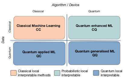
Figure 1: Categorization of interpretability techniques as they apply to classical and quantum resources. Here, the well-known QML diagram represents data, and an algorithm or device, which can be classical (C) or quantum (Q) in four different scenarios. We consider a reformulation of interpretable techniques to be required in the CQ scenario. In the QC and QQ quadrants, the design of explicitly quantum interpretable methods may be required. The scope of this paper covers CQ approaches.

In parallel, recent years have witnessed a surge of research efforts in quantum machine learning (QML) [9, 10]. This research area sits at the intersection of machine learning and quantum computing. The development of QML has undergone different stages. Initially, the field started with the quest for speedups or quantum advantages. More recently, the target has morphed into further pursuits in expressivity and generalization power of quantum models. Nowadays, rather than “competing” with classical models, quantum models are further being enhanced on their own, which could, in turn, improve classical machine learning techniques. One of the key techniques currently used in QML research is the variational quantum algorithm, which acts as the quantum equivalent to classical neural networks [11]. To clarify the analogy, we will refer to such models as quantum neural networks (QNNs) [12].

Given the close conceptual correspondence to classical neural networks, it is natural to analyze their interpretability, which is important for several reasons. Firstly, QNNs may complement classical AI algorithm design, making their interpretability at least as important as classical DNNs. Secondly, the quantum paradigms embedded into QNNs deserve to be understood and explained in their own right. The unique non-intuitive characteristics of quantum nature can make QNNs more complicated to interpret from the point of view of human understandability. Finally, with the growing interest and capabilities of quantum technologies, it is crucial to identify and mitigate potential sources of errors that plague conventional AI due to a lack of transparency.

In this work, we define some notions of the interpretability of quantum neural networks. In doing so, we generalize some well-known interpretable techniques to the quantum domain. Consider the standard relationship diagram in QML between data and algorithm (or device) type, where either can be classical (C) or quantum (Q). This entails the following combinations (CC, CQ, QC, and QQ), shown in Figure 1. Classical interpretable techniques are the apparent domain of CC. We will discuss, but not dwell on, the potential need for entirely new techniques when the data is quantum (QC and QQ). In CQ, the domain that covers the so-called quantum-enhanced machine learning techniques, although the data is classical, the output of the quantum devices is irreversibly probabilistic. Generalizing classical notions of interpretability to this domain is the subject of our work.

The question of interpretability in quantum machine learning models more broadly, as well as of QNNs more specifically, has already started to receive attention [13, 14, 15], particularly involving the concept of Shapley values [16], which attempt to quantify the importance of features in making predictions. In [13] interpretability is explored using Shapley values for quantum models by quantifying the importance of each gate to a given prediction. The complexity of computing Shapley values for generalized quantum scenarios is analyzed in [17]. In [15], Shapley values are computed for a particular class of QNNs. Our work complements these efforts using an alternative notion of explainability to be discussed in detail next.

II Interpretability in AI

II.1 Taxonomy

There are several layers to the design of interpretability techniques. To start, they can be model-specific or model-agnostic. As the name suggests, model-specific methods are more restrictive in terms of which models they can be used to explain. As such, they are designed to explain one single type of model. In contrast, model-agnostic methods allow for more flexibility in usage as they can be used on a wide range of model types. At large, model-agnostic methods can have a global or local interpretability dimension. Locality determines the scope of explanations with respect to the model. Interpretability at a global level explains the average predictions of the model as a whole. At the same time, local interpretability gives explanations at the level of each sample. In another axis, these techniques can be active (inherently interpretable) or passive (post-hoc). The state of these interpretable paradigms implies the level of involvement of interpretable techniques in the outcome of the other parameters. Active techniques change the structure of the model itself by leaning towards making it more interpretable. In contrast, passive methods explain the model outcome once the training has finished. In comparison to model-agnostic methods, which work with samples at large, there also exist example-based explanations which explain selected data samples from a dataset. An example of this method is the $k$-nearest neighbours models, which average the outcome of $k$ nearest selected points.

Other than the idea of building interpretable techniques, or more precisely, techniques that interpret various models, there exist models that are inherently interpretable. Such models include linear regression, logistic regression, naive Bayes classifiers, decision trees, and more. This feature makes them good candidates as surrogate models for interpretability. Based on this paradigm, there exists the concept of surrogate models, which uses interpretable techniques as a building block for designing other interpretable methods. Such important techniques are, for example, local interpretable model-agnostic explanations (LIME) [18] and Shapley additive explanations (known as SHAP) [16].

II.2 Interpretability of neural networks

The interpretability of neural networks remains a challenge on its own. This tends to amplify in complex models with many layers and parameters. Nevertheless, there is active research in the field and several proposed interpretable techniques [7]. Such techniques that aim to gain insights into the decision-making of a neural network include saliency maps [19], feature visualization [20, 21], perturbation or occlusion-based methods [18, 16], and layerwise relevance propagation (also known by its acronym LRP) [22].

To expand further on the abovementioned techniques, saliency maps use backpropagation and gradient information to identify the most influential regions contributing to the output result. This technique is also called pixel attribution [4]. Feature visualisation, particularly useful for convolutional natural networks, is a technique that analyses the importance of particular features in a dataset by visualising the patterns that activate the output. In the same remark, in terms of network visualisations, Ref. [23] goes deeper into the layers of a convolutional neural network to gain an understanding of the features. This result, in particular, shows the intricacies and the rather intuitive process involved in the decision-making procedure of a network as it goes through deeper layers. Occlusion-based methods aim to perturb or manipulate certain parts of the data samples to observe how the explanations change. These methods are important in highlighting deeper issues in neural networks. Similarly, layerwise relevance propagation techniques re-assign importance weight to the input data by analysing the output. This helps the understanding by providing a hypothesis over the output decision. Finally, the class of surrogate-based methods mentioned above is certainly applicable in neural networks as well.

The importance of these techniques is also beyond the interpretability measures for human understanding. They can also be seen as methods of debugging and thus improving the result of a neural network as in Ref. [23]. Below we take a closer look at surrogate model-agnostic local interpretable techniques, which are applicable to DNNs as well.

II.3 Local interpretable methods

Local interpretable methods tend to focus on individual data samples of interest. One of these methods relies on explaining a black-box model using inherently interpretable models, also known as surrogate methods. These methods act as a bridge between the two model types. The prototype of these techniques is the so-called local interpretable model-agnostic explanations (LIME), which has gotten much attention since its invention in 2016 [18]. Local surrogate methods work by training an interpretable surrogate model that approximates the result of the black-box model to be explained. LIME, for instance, categorizes as a perturbation-based technique that perturbs the input dataset. Locality in LIME refers to the fact that the surrogate model is trained on the data point of interest, as opposed to the whole dataset (which would be the idea behind global surrogate methods). Eq. (1) represents the explanation $\xi$ of a sample $x$ via its two main terms, namely the term $L(f,g,\pi_{x})$ representing the loss which is the variable to be minimized, and $\Omega(g)$ which is the complexity measure, which encodes the degree of interpretability. Here $f$ is the black-box model, $g$ is the surrogate model, and $\pi_{x}$ defines the region in data space local to $x$. In broader terms, LIME is a trade-off between interpretability and accuracy,

$$\xi(x)=\operatorname*{argmin}_{g\in G}L(f,g,\pi_{x})+\Omega(g)$$ (1)

In the following, we make use of the concept of local surrogacy to understand the interpretability of quantum models using LIME as a starting point. Much like LIME, we develop a framework to provide explanations of black-box models in the quantum domain. The class of surrogate models, the locality measure, and the complexity measure are free parameters that must be specified and justified in each application of the framework.

III The case for quantum AI interpretability

As mentioned in Section I, interpretability in the quantum literature in the context of machine learning can take different directions. We consider the case when data is classical and encoded into a quantum state, which is manipulated by a variational quantum circuit before outputting a classical decision via quantum measurement. Our focus is on interpreting the classical output of the quantum model.

A quantum machine learning model $f$ takes as input data $x$ and first produces quantum data $|\psi(x)\rangle$. A trained quantum algorithm — the QNN, say — then processes this quantum data and outputs a classification decision based on the outcome of a quantum measurement. This is not conceptually different from a classical neural network beyond the fact that the weights and biases have been replaced by parameters of quantum processes, except for one crucial difference — quantum measurements are unavoidably probabilistic.

Probabilities, or quantities interpreted as such, often arise in conventional neural networks. However, these numbers are encoded in bits and directly accessible, so they are typically used to generate deterministic results (through thresholding, for example). Qubits, on the other hand, are not directly accessible. While procedures exist to reconstruct qubits from repeated measurements (generally called tomography), these are inefficient — defeating any purpose of encoding information into qubits in the first place. Hence, QML uniquely forces us to deal with uncertainty in interpreting its decisions.

In the case of probabilistic decisions, the notion of a decision boundary is undefined. A reasonable alternative might be to define the boundary as those locations in data space where the classification is purely random (probability $\frac{1}{2}$). A data point here is randomly assigned a label. For such a point, any explanation for its label in a particular realization of the random decision process would be arbitrary and prone to error. It would be more accurate to admit that the algorithm is indecisive at such a point. This rationale is equally valid for data points near such locations. Thus, we define the region of indecision as follows,

$$R=\left\{x^{\prime}\in X:\left\lvert P(f(x^{\prime})=1)-\frac{1}{2}\right\rvert<\epsilon\right\},$$ (2)

where $\epsilon$ is a small positive constant representing a threshold of uncertainty tolerated in the classification decision. In some sense of the word, points lying within this reason have no explanation for their particular beyond “luck” — or unluck, depending on one’s point of view!

Now, while some data points have randomly assigned labels, we might still ask why. In other words, even data points lying within the region of indecision demand an explanation. Next, we will show how the ideas of local interpretability can be extended to apply to the probabilistic setting.

III.1 Probabilistic local interpretability

In the context of LIME, the loss function is typically chosen to compare models and their potential surrogates on a per-sample basis. However, if the model’s output is random, the loss function will also be a random variable. An obvious strategy would be to define loss via expectation:

$$\xi(x)=\operatorname*{argmin}_{g\in G}\mathbb{E}[L(f,g,\pi_{x})]+\Omega(g).$$ (3)

However, even then, we still cannot say that $\xi$ is an explanation, as its predictions are only capturing the average behaviour of the underlying model’s randomness. In fact, the label provided by $\xi$ may be the opposite of that assigned to $x$ by the model in any particular instance!

To mitigate this, we call an explanation the distribution $\Xi$ of trained surrogate models $g$. Note again that $g$ is random, trained on synthetic local data with random labels assigned by the underlying model. Thus, the explanation inherits any randomness from the underlying model. It’s not the case that the explanation provides an interpretation of the randomness per se — however, we can utilize the distribution of surrogate models to simplify the region of indecision, hence providing an interpretation of it.

III.2 Band of inexplicability

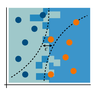
Figure 2: Depiction of the concept of the band of inexplicability. The space within the dashed lines represents the region in the decision space where data samples exhibit ambiguous classification due to randomness. The figure showcases a two-class classification task in a two-dimensional space with two features represented along the horizontal and vertical axes. Here, $\epsilon$ is the pre-defined threshold. Likely, data samples either inside or close by the band, can not be explained.

In this section, we define the band of inexplicability. Loosely speaking, this is the region of indecision interpreted locally through a distribution of surrogate models. Suppose a particular data point lies within its own band of inexplicability. The explanation for its label is thus there is no explanation. Moreover, this is a strong statement because — in principle — all possible interpretable surrogate models have been considered in the optimization.

The band of inexplicability can be defined as the region of the input space where the classification decision of the quantum model is uncertain or inexplainable. More formally, we can define the band of inexplicability $B$ for a data point $x$ in a dataset $X$ as,

$$B=\left\{x^{\prime}\in X:\left\lvert P(g(x^{\prime})=1|f,\Xi,\pi_{x})-\frac{1}{2}\right\rvert<\epsilon\right\},$$ (4)

where $\epsilon$ is again a small positive constant representing a threshold of uncertainty tolerated in the classification decision — this time with reference to the explanation rather than the underlying model. Note that the distribution in Eq. (4) is over $\Xi$ as each $g$ provides deterministic labels.

In much the same way that an interpretable model approximates decision boundaries locally in the classical context, a band of inexplicability approximates the region of indecision in the quantum (or probabilistic) context. The size and shape of this region will depend on several factors, such as the choice of the interpretability technique, the complexity of the surrogate model, and the number of features in the dataset. We call the region a “band” as it describes the simplest schematic presented in Fig. 2.

IV Numerical experiments for interpreting QNNs

We use the well-known Iris dataset [24] for our numerical experiments. For the sake of the explainability of our own method (no pun intended), we reduce it to a binary classification problem, using only two of the three classes in this dataset as well as only two of the four features. Since we don’t actually care about classifying flowers here, with apologies to iris lovers, we abstract the names of these classes and labels below.

The trained quantum model to be explained is a hybrid QNN trained using simultaneous perturbation stochastic approximation (better known by its acronym SPSA) built and simulated using the Qiskit framework [25]. Each data point is encoded into a quantum state with the angle encoding [26]. The QNN model is an autoencoder with alternating layers of single qubit rotations and entangling gates [27]. Since our goal here is to illustrate the band of inexplicability, as in Eq. 4, we do not optimize over the complexity of surrogate models and instead fix our search to the class of logistic regression models with two features.

The shaded background in each plot of Figs. 3 and 4 show the decision region of the trained QNN. Upon inspection, it is clear that these decision regions, and the implied boundary, change with each execution of the QNN. In other words, the decision boundary is ill-defined. In Fig. 3, we naively apply the LIME methodology to two data points — one in the ambiguous region and one deep within the region corresponding to one of the labels. In the latter case, the output of the QNN is nearly deterministic in the local neighbourhood of the chosen data point, and LIME works as expected — it produces a consistent explanation.

However, in the first example, the data point receives a random label. It is clearly within the region of indecision for a reasonably small choice of $\epsilon$. The “explanation” provided by LIME (summarized by its decision boundary shown as the solid line in Fig. 3) is random. In other words, each application of LIME will produce a different explanation. For the chosen data point, the explanation itself produces opposite interpretations roughly half the time, and the predictions it makes are counter to the actual label provided by the QNN model to be explained roughly half the time. Clearly, this is an inappropriate situation to be applying such interpretability techniques. Heuristically, if a data point lies near the decision boundary of the surrogate model for QNN, we should not expect that it provides a satisfactory explanation for its label. The band of inexplicability rectifies this.

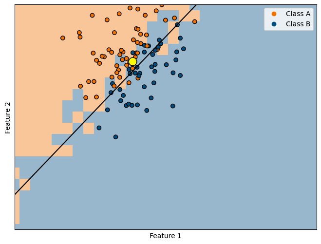
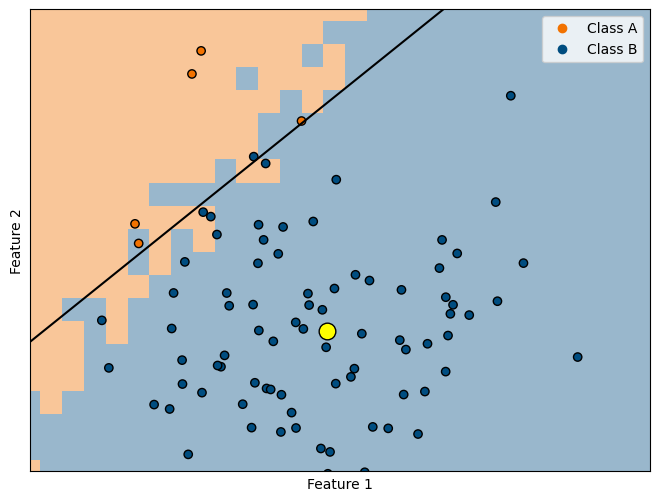
Figure 3: The classification uncertainty for a chosen data sample (yellow). The two shadings represent the decision boundary of the QNN, which is clearly randomly defined. The synthetic data and the produced surrogate linear decision boundary are shown for a single instance of QNN labels. (top) A clear example of an undefined classification result for the selected data point. (bottom) Decision boundary unambiguously separates the who classes with respect to the selected data point.

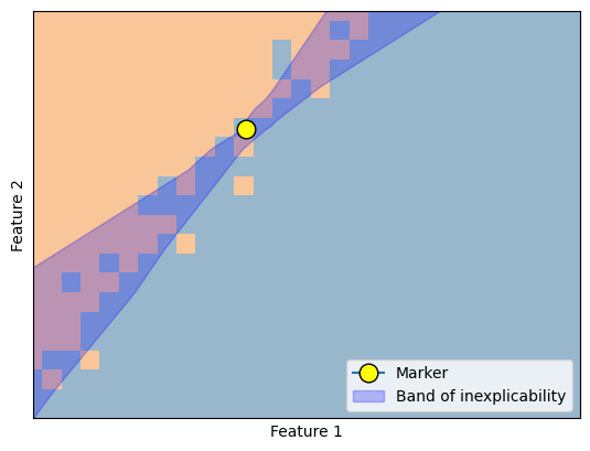
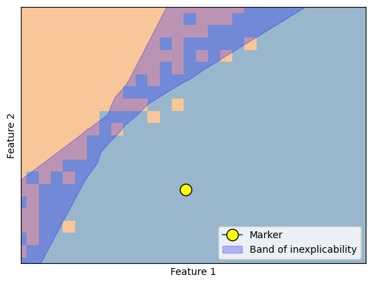
Figure 4: The approximated band of inexplicability. (top) An example of a marked data point that lies on the band of inexplicability. (bottom) A data point that is outside of this region and hence can be assessed for interpretability as per the interpretable techniques.

For the same sample data points, the band of inexplicability is shown in Fig. 4. Data points within their own band should be regarded as having been classified due purely to chance — and hence have no “explanation” for the label they have been assigned. Note that the band itself is unlikely to yield to analytic form. Hence, some numerical approximation is required to calculate it in practice. Our approach, conceptually, was to repeat what was done to produce Fig. 3 many times and summarize the statistics to produce Fig. 4. A more detailed description follows, and the implementation to reproduce the results presented here can be found at [28].

Abstractly, approximating the band of inexplicability requires a trained QNN, a sample data point, a function defining “local,” and some meta-parameters defining the quality of the numerical approximation, such as the amount of synthetic data to be used and the number of Monte Carlo samples to take. Once these are defined, the pseudocode is as follows:

1. Create synthetic data locally around the chosen data point;

2. Apply LIME to generate a surrogate model;

3. Repeat 1 and 2 several times to produce an ensemble of decision boundaries.

4. Take the interquartile range (say) of those boundaries.

To be clear, Fig 3 is produced through a single application of steps 1 and 2 while Fig. 4 is produced after the final step. Note that in a “real” application, it would be infeasible to plot the decision regions to any reasonable level of accuracy. This makes the band of indecision both valuable and convenient in interpreting QNNs.

V Discussion

In summary, in interpreting the classification output of a QNN, we have defined the band of inexplicability, a simple description of a region where the QNN is interpreted to be indecisive. The data samples within their associated band should not be expected to have an “explanation” in the deterministic classical sense. While directly useful for hybrid quantum-classical models, we hope this stimulates further research on the fundamental differences between quantum and classical model interpretability. In the remainder of the paper, we discuss possible future research directions.

Our results are pointed squarely at the randomness of quantum measurements, which might suggest that they are “backwards compatible” with classical models. Indeed, randomness is present in training classical DNNs due to random weight initialization or the optimization techniques used. However, this type of randomness can be “controlled” via the concept of a seed. Moreover, the penultimate output of DNNs (just before label assignment) is often a probability distribution. However, these are produced through arbitrary choices of the activation function (i.e., the Softmax function), which force the output of a vector that merely resembles a probability distribution. Each case of randomness in classical DNNs is very different from the innate and unavoidable randomness of quantum models. While our techniques could be applied in a classical setting, the conclusions drawn from them may ironically be more complicated to justifiably action.

In this work, we have provided concrete definitions for QNNs applied to binary classification problems. Using a probability of $\frac{1}{2}$ would not be a suitable reference point in multi-class decision problems. There are many avenues to generalize our definitions which would mirror standard generalizations in the move from binary to multi-class decision problems. One such example would be defining the region of indecision as that with nearly maximum entropy.

We took as an act of brevity the omission of the word local in many places where it may play a pivotal role. For example, the strongest conclusion our technique can reach is that a QNN is merely locally inexplicable. In such cases, we could concede that (for some regions of data space) the behaviour of QNN is inexplicable, full stop. Or we can use the conclusion to signal that an explanation at a higher level of abstraction is required. Classically, a data point asks, “Why give me this label?” Quantumly, our answer might be, “Sorry, quantum randomness.” Yet, the data point may persist, “But what about me led to that?” These may be questions that a quantum generalization of global interpretability techniques could answer.

Referring back to Fig. 1, we have focused here on CQ quantum machine learning models. However, the core idea behind local surrogate models remains applicable in the context of quantum data — use interpretable quantum models as surrogate models to explain black box models producing quantum data. Of course, one of our assumptions is the parallels between the classical interpretable models we mentioned above, with their quantum equivalents. This can be a line for future work. The ideas here encapsulate inherently quantum models such as matrix product states or tensor network states, which can act as surrogate models for quantum models as they may be considered more interpretable.

Furthermore, the idea behind interpreting or “opening up” black-box models may be of interest in control theory [29, 30, 31]. In this scenario, the concept of “grey-box” models — portions of which encode specific physical models — give insights into how to engineer certain parameters in a system. These grey-box models can thus be considered partially explainable models. The proposed algorithm in [32] may also be of interest in terms of creating intrinsically quantum interpretable models, which would act as surrogates for other more complex quantum models.

An obvious open question that inspires future research remains to investigate the difference in computational tractability of interpretability methods in quantum versus classical. This will lead to understanding whether it is more difficult to interpret quantum models as opposed to classical models. We hope such results shed light on more philosophical questions as well, such as is inexplicability, viz. complexity, necessary for learning?.

For completeness, the case for the interpretability of machine learning models does not go without critique. There are opinions that performance should not be compromised in order to gain insights into the decision-making of the model, and realistically it may not always be prioritized [33, 34]. Simple models tend to be more explainable, however, it is the more complex models that require explanations, as they may be more likely employed in critical applications.

Regardless of the two distinct camps of beliefs, the niche field of interpretable machine learning keeps growing in volume. An argument is that having a more complete picture of the model’s performance can help improve the performance of the model overall. As QML becomes more relevant to AI research, the need for quantum interpretability, we expect, will also be in demand.

Acknowledgments: LP was supported by the Sydney Quantum Academy, Sydney, NSW, Australia.

References

- Russell and Norvig [2010] S. Russell and P. Norvig, Artificial Intelligence: A Modern Approach, 3rd ed. (Prentice Hall, 2010).
- Mitchell [1997] T. M. Mitchell, Machine Learning, 1st ed. (McGraw-Hill, Inc., USA, 1997).
- Molnar [2022] C. Molnar, Interpretable Machine Learning, 2nd ed. (2022).
- Molnar et al. [2020] C. Molnar, G. Casalicchio, and B. Bischl, Interpretable machine learning – a brief history, state-of-the-art and challenges, in ECML PKDD 2020 Workshops (Springer International Publishing, 2020) pp. 417–431.
- Lipton [2018] Z. C. Lipton, The mythos of model interpretability, Queue 16, 31 (2018).
- Goodfellow et al. [2016] I. Goodfellow, Y. Bengio, and A. Courville, Deep Learning (MIT Press, 2016) http://www.deeplearningbook.org.
- Zhang et al. [2021] Y. Zhang, P. Tino, A. Leonardis, and K. Tang, A survey on neural network interpretability, IEEE Transactions on Emerging Topics in Computational Intelligence 5, 726 (2021).
- Guidotti et al. [2018] R. Guidotti, A. Monreale, S. Ruggieri, F. Turini, F. Giannotti, and D. Pedreschi, A survey of methods for explaining black box models, ACM computing surveys (CSUR) 51, 1 (2018).
- Biamonte et al. [2016] J. Biamonte, P. Wittek, N. Pancotti, P. Rebentrost, N. Wiebe, and S. Lloyd, Quantum Machine Learning, Nature 549, 195 (2016).
- Schuld and Petruccione [2021] M. Schuld and F. Petruccione, Machine Learning with Quantum Computers (Springer International Publishing, 2021).
- Cerezo et al. [2022] M. Cerezo, G. Verdon, H.-Y. Huang, L. Cincio, and P. Coles, Challenges and opportunities in quantum machine learning, Nature Computational Science (2022).
- Cerezo et al. [2021] M. Cerezo, A. Arrasmith, R. Babbush, S. C. Benjamin, S. Endo, K. Fujii, J. R. McClean, K. Mitarai, X. Yuan, L. Cincio, and P. J. Coles, Variational quantum algorithms, Nature Reviews Physics 3, 625 (2021).
- Heese et al. [2023] R. Heese, T. Gerlach, S. Mücke, S. Müller, M. Jakobs, and N. Piatkowski, Explaining quantum circuits with shapley values: Towards explainable quantum machine learning, arXiv preprint arXiv:2301.09138 10.48550/arXiv.2301.09138 (2023).
- Mercaldo et al. [2022] F. Mercaldo, G. Ciaramella, G. Iadarola, M. Storto, F. Martinelli, and A. Santone, Towards explainable quantum machine learning for mobile malware detection and classification, Applied Sciences 12, 10.3390/app122312025 (2022).
- Steinmüller et al. [2022] P. Steinmüller, T. Schulz, F. Graf, and D. Herr, explainable ai for quantum machine learning, arXiv preprint arXiv:2211.01441 10.48550/arXiv.2211.01441 (2022).
- Lundberg and Lee [2017] S. M. Lundberg and S.-I. Lee, A unified approach to interpreting model predictions, in Advances in Neural Information Processing Systems, Vol. 30 (Curran Associates, Inc., 2017).
- Burge et al. [2023] I. Burge, M. Barbeau, and J. Garcia-Alfaro, A quantum algorithm for shapley value estimation, arXiv preprint arXiv:2301.04727 10.48550/arXiv.2301.04727 (2023).
- Ribeiro et al. [2016] M. T. Ribeiro, S. Singh, and C. Guestrin, ”why should i trust you?”: Explaining the predictions of any classifier, in Proceedings of the 22nd ACM SIGKDD International Conference on Knowledge Discovery and Data Mining, KDD ’16 (Association for Computing Machinery, New York, NY, USA, 2016) p. 1135–1144.
- Simonyan et al. [2013] K. Simonyan, A. Vedaldi, and A. Zisserman, Deep inside convolutional networks: Visualising image classification models and saliency maps, arXiv preprint arXiv:1312.6034 10.48550/arXiv.1312.6034 (2013).
- Olah et al. [2017] C. Olah, A. Mordvintsev, and M. Tyka, Feature visualization: How neural networks build up their understanding of images, Distill 2 (2017).
- Yosinski et al. [2015] J. Yosinski, J. Clune, A. Nguyen, T. Fuchs, and H. Lipson, Understanding neural networks through deep visualization, in Proceedings of the 32nd International Conference on Machine Learning (ICML) (2015) pp. 1582–1591.
- Bach et al. [2015] S. Bach, A. Binder, G. Montavon, F. Klauschen, K.-R. Müller, and W. Samek, On pixel-wise explanations for non-linear classifier decisions by layer-wise relevance propagation, PLoS ONE 10, 10(7): e0130140 (2015).
- Zeiler and Fergus [2014] M. D. Zeiler and R. Fergus, Visualizing and understanding convolutional networks, European conference on computer vision , 818 (2014).
- Fisher [1936] R. A. Fisher, The use of multiple measurements in taxonomic problems (1936).
- IBM [2021] IBM, Qiskit: An Open-Source Framework for Quantum Computing (2021), accessed on May 1, 2023.
- Schuld and Petruccione [2018] M. Schuld and F. Petruccione, Supervised Learning with Quantum Computers, Quantum Science and Technology (Springer International Publishing, 2018).
- Farhi and Neven [2018] E. Farhi and H. Neven, Classification with quantum neural networks on near term processors, arXiv preprint arXiv:1802.06002 10.48550/arXiv.1802.06002 (2018).
- Pira and Ferrie [2023] L. Pira and C. Ferrie, Interpret QNN: Explicability and Inexplicability in the Interpretation of Quantum Neural Networks, https://github.com/lirandepira/interpret-qnn (2023), accessed on July 24, 2023.
- Youssry et al. [2023a] A. Youssry, Y. Yang, R. J. Chapman, B. Haylock, F. Lenzini, M. Lobino, and A. Peruzzo, Experimental graybox quantum system identification and control, arXiv preprint arXiv:2206.12201 10.48550/arXiv.2206.12201 (2023a).
- Youssry et al. [2020] A. Youssry, G. A. Paz-Silva, and C. Ferrie, Characterization and control of open quantum systems beyond quantum noise spectroscopy, npj Quantum Information 6, 95 (2020).
- Youssry et al. [2023b] A. Youssry, G. A. Paz-Silva, and C. Ferrie, Noise detection with spectator qubits and quantum feature engineering, New Journal of Physics 25, 073004 (2023b).
- [32] G. Weitz, L. Pira, C. Ferrie, and J. Combes, Sub-universal variational circuits for combinatorial optimization problems, In preparation.
- Sarkar [2022] A. Sarkar, Is explainable AI a race against model complexity?, arXiv preprint arXiv:2205.10119 10.48550/arXiv.2205.10119 (2022).
- McCoy et al. [2022] L. McCoy, C. Brenna, S. Chen, K. Vold, and S. Das, Believing in Black Boxes: Must Machine Learning in Healthcare Be Explainable to Be Evidence-Based?, Journal of Clinical Epidemiology 10.1016/j.jclinepi.2021.11.001 (2022).