PMVC: Data Augmentation-Based Prosody Modeling for Expressive Voice Conversion

Abstract.

Voice conversion as the style transfer task applied to speech, refers to converting one person’s speech into a new speech that sounds like another person’s. Up to now, there has been a lot of research devoted to better implementation of VC tasks. However, a good voice conversion model should not only match the timbre information of the target speaker, but also expressive information such as prosody, pace, pause, etc. In this context, prosody modeling is crucial for achieving expressive voice conversion that sounds natural and convincing. Unfortunately, prosody modeling is important but challenging, especially without text transcriptions. In this paper, we firstly propose a novel voice conversion framework named ‘PMVC’, which effectively separates and models the content, timbre, and prosodic information from the speech without text transcriptions. Specially, we introduce a new speech augmentation algorithm for robust prosody extraction. And building upon this, mask and predict mechanism is applied in the disentanglement of prosody and content information. The experimental results on the AIShell-3 corpus supports our improvement of naturalness and similarity of converted speech.

1. Introduction

Voice Conversion(VC), also called voice style transfer, aims to modify the voice characteristic of the source speech to convert one speaker’s voice to generate a new target speech as it is said by another people. It covers a wide range of applications like intelligent security products and aids. So far, many algorithms have made much progress in VC successfully (Stylianou et al., 1998; Goodfellow et al., 2014; Hsu et al., 2016; Baevski et al., 2019; Zhou et al., 2022). One of the most popular methods is to achieve VC tasks by separating the content and timbre information of speech to learn the disentangled speech representations (Nguyen and Cardinaux, 2022; Ding and Gutierrez-Osuna, 2019; Tang et al., 2021; Baevski et al., 2019). Specifically, these algorithms usually follow the autoencoder framework, and the encoder is trained to learn to represent content information and the timbre information, respectively. At the same time, a decoder is trained to output a natural speech from given content and timbre representations. With the pretrained autoencoder, we only need to replace the timbre representations of the source speech with that of the target speech before fed into decoder to generate the converted result.

Although these algorithms can easily implement VC tasks, few of them can convert all voice characteristics as expected (Polyak and Wolf, 2019a), such as the prosodic information. In fact, with previous algorithms, we can observe that almost all converted speech have the same pace, pause, and pitch contour shape as the source speech no matter what these voice characteristics of the target speech. In other words, previous methods convert only timbre, not all voice characteristics. Nowadays, VC not only demands high naturalness but also requires sufficient expressiveness in various scenarios, such as automatic movie dubbing with emotional conversations. Hence, with the advancement of deep learning, prosody modeling for expressive voice conversion has gradually attracted more and more attention (Xie et al., 2021; Wang et al., 2018; Qian et al., 2020, 2021). Its introduction greatly enriches the diversity and expressiveness of converted speech. Integrating prosody modeling into VC models provides basic framework for fine-tunning to carry out downstream tasks like emotional speech processing (Tang et al., 2023c, a). Specifically, a speech can be roughly decomposed into three components: the content information, which characterizes the phoneme and linguistic information; The timbre information, which is closely related to the speaker identity; Besides, the pace, pause and rhythm of a speech, which we call all of them the prosodic information. Obviously, in order to improve the expressiveness of voice conversion, compared with the simple division of speaker-independent and speaker-related information, we need to further model the content, timbre, and prosodic information, respectively.

In this paper, we introduce data augmented-based Prosody Modeling Voice Conversion (PMVC) model, which performs expressive voice conversion based on a novel speech augmentation algorithm. PMVC utilizes adaptive instance normalization in its encoder to eliminate the global static information from the speech. In addition, some information-theory-guided approaches are used to model the disentangled linguistic and prosodic features efficiently. Unlike many other previous models, PMVC models the prosody features without any text transcriptions. It significantly simplifies the complexity of the model and allows the prosody representation to contain richer information about the expressiveness of the phoneme rather than just the phoneme duration.

2. Related Work

2.1. Voice Conversion

Voice conversion (VC) is a task that aims to transfer speaking style of input speech while preserving content information. GAN-based methods (Kaneko and Kameoka, 2018; Kameoka et al., 2018) are employed to perform VC task with advantages of high efficiency and diversity. Speaking style is regarded as a condition and injected into generation process. However, such training process lacks of controllability.

Hence, disentanglement based VC methods have aroused people’s attention. Qian et. al. first proposed AutoVC (Qian et al., 2019), by applying the bottleneck structure, AutoVC can force the encoder to discard some information of the input speech to learn the disentangled content representation. Vector quantization (VQ) based methods (Tang et al., 2022, 2023d) and adversarial training based methods (Tang et al., 2023b) are also introduced for better disentanglement. Then Studies have been conducted to explore more voice characteristics for expressiveness, such as prosody.

2.2. Prosody Modeling

Proosdy modeling is crucial yet challenging. The causes of this complexity are multifaceted, and one critical reason is the difficulty in completely eliminating prosodic information from the source speech. As (Zhou et al., 2021) said, prosodic features are often closely associated with phonemes, so it is difficult to separate them and model them individually. Currently, prosody modeling methods are predominantly present in expressive text-to-speech (TTS) systems. Previous work (Skerry-Ryan et al., 2018) introduced a Tacotron-based method capable of disentangling prosody from speech content. Mellotron (Valle et al., 2020) further extracts different aspects of the prosodic information. Besides, CHiVE (Kenter et al., 2019) is also proposed to extract and learn prosody features for expressive TTS. Recently, prosody modeling is also applied to VC tasks. Parrotron (Biadsy et al., 2019) extract prosodic information by encouraging the latent code to be the same as the phoneme embeddings, IQDUBBING (Gan et al., 2022) use a prosody extracter and two prosody filter to extract the prosodic features. However, all of the above methods require text transcriptions. Of course, with text transcriptions, prosody modeling can be easier, but it also limits their ability to scale to those speech corpus that don’t have text transcriptions.

To further improve the expressiveness of VC, SpeechFlow (Qian et al., 2020) achieves the disentanglement of the voice characteristics like content, timbre, rhythm and pitch information from the input speech. Besides, by defining prosodic information as the duration of a phoneme, AutoPST (Qian et al., 2021) achieves the global rhythm transfer without any text transcriptions. Both SpeechFlow and AutoPST necessitate imposing stringent constraints on the dimensions of the latent embedding to achieve a proper balance between timbre disentanglement and intelligibility. It’s related to the final quality of conversion and poses challenges for direct application to other datasets.

To issue this problem, in this paper, we first discard the bottleneck structure. At the same time, we introduce the Instance Normalization layer to achieve a similar function of filtering timbre information. In fact, previous studies have shown that Instance normalization(IN) can eliminate the speaker information without introducing any information bottleneck structure (Ulyanov et al., 2016; Wang et al., 2020). Recently, INVC (Chou and Lee, 2019) separated the speaker and content representations by applying the adaptive instance normalization. However, as we said before, IN just eliminates the global timbre information, and the time-variant representations still contain the phoneme and prosodic information. We still need an effective method to extract the prosodic features from the content representations.

Inspired by (Tang et al., 2022), we proposed a new method that utilizes contrastive learning to disentangle the content embeddings and the prosody embeddings from the time-variant representations. In order to implement this method, we need to first construct the augmented speech of the original speech.

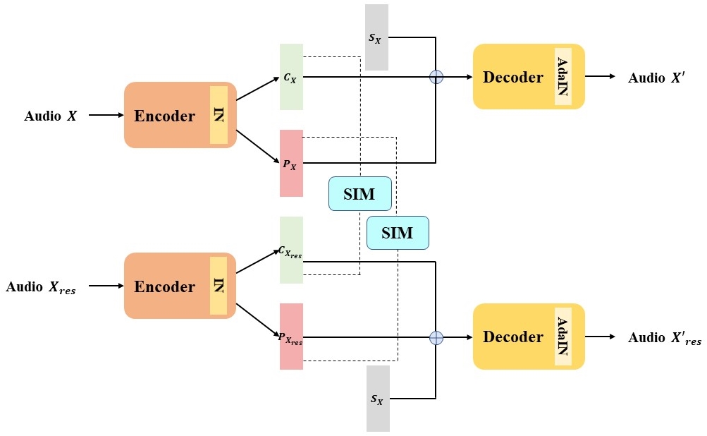
(a) Framework of PMVC

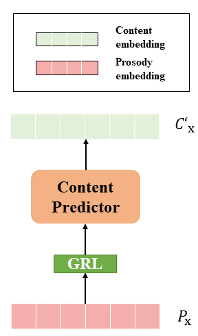
(b) Content predictor

Figure 1. Framework of PMVC. $\boldsymbol{C}_{x}$ and $\boldsymbol{P}_{x}$ are the content features and prosodic features extracted from the input speech. Denote $\boldsymbol{S}_{x}$ as speaker embedding, generated from the pretrained speaker encoder. $\boldsymbol{IN}$, $\boldsymbol{AdaIN}$ stand for Instance Normalization and adaptive instance normalization, respectively. Which can eliminate the global static information from $\boldsymbol{x}$. The right image shows the content predictor. $\boldsymbol{C}^{\prime}_{x}$ denotes the predicted content embedding, it’s reasonable to expect a close association with $\boldsymbol{C}_{x}$. GRL means Gradient Reversal Layer, it will make the optimization goal of the feature encoder and the content predictor completely opposite.

3. Proposed Methods

As depicted in Figure 1(a), the framework of PMVC includes three main modules. The first one is a feature encoder $E$, responsible for the extraction of content feature $\boldsymbol{C}$ and the prosody feature $\boldsymbol{P}$ from the input speech $\boldsymbol{X}$. $IN$ in $E$ means Instance Normalization, and it can remove the global static information from $\boldsymbol{X}$. Instead, a pretrained speaker encoder $E_{s}$ is introduced to provide the speaker embedding $\boldsymbol{S}$. With the disentangled content embedding, prosody embedding, and the speaker embedding, a decoder $D$ is trained to output a natural reconstructed speech $\boldsymbol{X^{\prime}}$.

3.1. Stretching Audio Time Series Strategy

In this paper, the spectrogram of the original audio time series is denoted as $X(T)$, where $T$ represents the frame number. Then, we define the content vector $C$ to represent the content information, the prosody vector $P$ to represent the prosodic information, and we define the timbre vector $S$ as the speaker-related information. Based on our assumption, for each speech segment $X$, it can be uniquely determined by given the disentangled speech representations $C$, $P$ and $S$. Formally, $X$ can be considered a random variable sampled from the speech distribution $p_{x}(\cdot|C,P,S)$.

As mentioned in SpeechFlow (Qian et al., 2020), Random Resampling (RR) operation is an effective strategy to change the prosodic information of the original audio time series. Specifically, RR involves three steps of operations. The initial step involves dividing the input audio series into segments of random lengths. Then, the second step is to randomly draw a sampling rate for each segment. And, the last step is to re-sample the segment with the selected sampling rate. Compared with the original audio sequence $X$, the output audio sequence $X_{RR}$ retains the original content, but changes the timbre and prosodic information. It can be expressed as:

$$\boldsymbol{X} \sim p_{X}(\boldsymbol{\cdot|C=C_{X},P=P_{X},S=S_{X}}).$$

(1) $$\boldsymbol{X_{RR}} \sim p_{X_{RR}}(\boldsymbol{\cdot|C=C_{X},P=P_{X_{RR}},S=S_{X_{RR}}})$$

Noted that after random resampling, the sequence length of the audio may also be changed. To address this problem, existing methods align the lengths of $X$ and $X_{RR}$ by using a padding constant of 0 (Qian et al., 2020; Polyak and Wolf, 2019b). However, it will inevitably affect the data quality, thereby increasing the difficulty of model training. Besides, in order to make prosodic modeling more convenient, we expect to find a new algorithm that can change the prosodic information but remain the original timbre and content, that is, Time scale modification (TSM).

Algorithm 1 Random Prosody Algorithm

Input: A speech segment $\boldsymbol{X}$ of length $T$

Parameter: The split length $\boldsymbol{t}$, sampling rate $R$

Output: RR speech segment $\boldsymbol{X_{res}}$ with same length $T$

1:  Let $num=T/t$. We divide $\boldsymbol{X}$ into $num$ segments with the same length $\boldsymbol{t}$, $L=[x_{1},x_{2},...x_{num}]$

2:  while $num>1$ do

3:     Select two segments $\boldsymbol{x_{i}}$ and $\boldsymbol{x_{j}}$ from $L$

4:     $a=Uniform(0.6,2)$

5:     Stretch audio time series $\boldsymbol{x_{i}}$ with the specific rate $a$

6:     Stretch audio time series $\boldsymbol{x_{j}}$ with the specific rate $\frac{a}{2a-1}$

7:     Remove $\boldsymbol{x_{i}}$ and $\boldsymbol{x_{j}}$ from $L$

8:     $num=num-2$

9:  end while

10:  $\boldsymbol{X_{res}}$ is obtained by concatenating all speech segments in the original order

11:  return $\boldsymbol{X_{res}}$

Inspired by it, this paper proposes a new method that guides the learning of disentanglement speech representations with information-theory-guided constraints. Specifically, we first propose a new strategy of stretching audio time series, which can be roughly divided into three steps. As shown in Algorithm 1, first, the input sequence is segmented into uniform-length segments. Second, for each pair of segments selected randomly, a rate is randomly drawn, and the total sample points of the sequence segments remain the same (one segment is stretched, and the other is correspondingly shortened). Finally, we stitch all the speech fragments together in the previous order. With this algorithm, for each sequence $x$, we can get a corresponding augmented speech $x_{res}$ with the same length $T$. And it can be expressed as:

(2) $$\boldsymbol{X_{res}}\sim p_{X_{res}}(\boldsymbol{\cdot|C=C_{X},P=P_{X_{res}},S=S_{X}})$$

And based on the augmented data, a new method has been proposed to extract the prosodic information from speech.

3.2. How to Train The Model

Here we will present how and why our model can induce the content embedding and prosody embedding into independent representation spaces simultaneously.

As we discussed before, $\boldsymbol{X_{res}}$ can be regarded as an augmented speech of $\boldsymbol{X}$. That is, $\boldsymbol{X_{res}}$ and $\boldsymbol{X}$ have the same content information, same timbre information and different prosodic information. During training, a pair of speech segments ($\boldsymbol{x,x_{res}}$) are selected to be the input, the feature encoder $E$ can eliminate the global speaker information while preserving other information from the input speech by using instance normalization without affine transformation, and it can be expressed as:

(3) $$\mu_{c}=\frac{1}{W}\sum_{w=1}^{W}M_{c}[w]$$

(4) $$\alpha_{c}=\sqrt{\frac{1}{W}\sum_{w=1}^{W}(M_{c}[w]-\mu_{c})^{2}+\epsilon}$$

(5) $$Z_{c}[w]=\frac{M_{c}[w]-\mu_{c}}{\alpha_{c}}$$

where $M_{c}$ is the feature map in $c$-th channel, $W$ denote as the dimension of $M_{c}$, $M_{c}[w]$ is the $w$-th element in $M_{c}$, $Z_{c}[w]$ refer to the normalized $M_{c}[w]$. Besides, $\epsilon$ is a small value which can avoid numerical instability.

Obviously, the normalized hidden feature $Z$ contains both content information and prosodic information. We further hypothesize that $Z$ is a specific expression composed of the estimated content embedding $\boldsymbol{C_{x}}$ and estimated prosody embedding $\boldsymbol{P_{x}}$:

(6) $$\boldsymbol{Z}=E(\boldsymbol{x})=\boldsymbol{C_{x}}\oplus\boldsymbol{P_{x}}$$

where $\oplus$ means concatenation. In this scenario, we split $\boldsymbol{Z}$ along the channel dimensions, representing the estimated content embedding $\boldsymbol{C_{x}}$ and the estimated prosody embedding $\boldsymbol{P_{x}}$ respectively.

Since $\boldsymbol{x}$ and $\boldsymbol{x_{res}}$ have the same content information, their content embeddings are expect to be as closer as possible. At the same time, after Random Prosody (RP) operation, the prosodic information of $\boldsymbol{x}$ have been corrupted. In other words, the prosodic information in $\boldsymbol{x}$ and $\boldsymbol{x_{res}}$ should be different. Hence, we expect their prosody embeddings should be as different as possible. However, although $\boldsymbol{x}$ and $\boldsymbol{x_{res}}$ contain the same semantic information, the phoneme of each frame may be different (otherwise $\boldsymbol{x}$ and $\boldsymbol{x_{res}}$ will be exactly the same). So, unlike most similar studies, MSE loss or L1 loss cannot be applied here. Specially, we employ cosine similarity to measure the similarity between a pair of features in this paper:

(7) $$G(A(x),A(x_{res}))=\frac{A^{T}(x)A(x_{res})}{\|A(x)\|_{2}\|A(x_{res})\|_{2}}$$

where $G(\cdot,\cdot)$ represents the calculation of cosine similarity score. $A(\cdot)$ can be used to represent any extracted embedding of input speech.

As mentioned, the training of the proposed model aims to maximize cosine similarity between similar content embeddings, and minimize it between the different prosody embeddings. Hence, the proposed similarity contrastive loss function for model training is:

(8) $$\mathcal{L_{\text{sim}}}=\frac{G(P(x),P(x_{res}))}{G(C(x),C(x_{res}))}$$

Besides, the speaker embedding $S_{x}$ is produced by a pretrained speaker encoder with GE2E loss (Wan et al., 2018). It involves positive pairs composed of different utterances of the same speaker and negative pairs composed of different speakers. The embedding similarity of positive pairs needs to be maximized, and the similarity of negative pairs needs to be minimized during pretraining. We can easily find that the speaker embedding contains only the timbre information. Here we will give a formal discussion about the speaker embedding: We assume that there are two speakers $S1$ and $S2$ and some of their speeches. As we discussed before, for each speech $X$ belong to speaker $S$, it can be formulated as:

$$\boldsymbol{X} \sim p_{X}(\boldsymbol{\cdot|C=C,P=P,S=S}).$$

Now, assume there are two speeches $x1$ and $x2$, both from the same speaker $S1$. And, there are another speech $x3$ belongs to another speaker $S2$. It can be expressed as:

$$\boldsymbol{x1} \sim p_{X}(\boldsymbol{\cdot|C=C_{x1},P=P_{x1},S=S1}).$$

$$\boldsymbol{x2} \sim p_{X}(\boldsymbol{\cdot|C=C_{x2},P=P_{x2},S=S1}).$$

$$\boldsymbol{x3} \sim p_{X}(\boldsymbol{\cdot|C=C_{x3},P=P_{x3},S=S2}).$$

Note that the content and prosody information of each speech here are random. For the convenience of discussion, we assume that the content information of $x1$ and $x3$ are the same. In other words, the only difference between $x1$ and $x3$ are the timbre information and part of prosody information. In training, we expect the speaker encoder can output different embeddings from $x1$ and $x3$. Then, the most convenient way for the speaker encoder in training is to discard the content information and extract the timbre and prosodic features.

At the same time, we can further assume that the prosody information in $x1$ and $x2$ are different. In training, we expect the speaker encoder would output the same embeddings from $x1$ and $x2$. In this case, the encoder would be encouraged to discard the prosody information and extract the timbre and part of the content features.

In summary, the speaker encoder will learn to extract only the timbre information in the speech, while eliminating the content and prosody information as much as possible. So we say the speaker embeddings contain only the timbre information.

Finally, leveraging the content embedding $C_{x}$, prosody embedding $P_{x}$, and speaker embedding $S_{x}$, the decoder is guided to produce the reconstructed speech $x^{\prime}$. We employ a reconstruction loss function during training, which is as follows:

(9) $$\mathcal{L}_{\text{recon }} =\|x^{\prime}-x\|_{2}^{2}+\|x^{\prime}_{res}-x_{res}\|_{2}^{2}$$

where $x^{\prime}$ is generated from $C_{x}$, $P_{x}$ and $S_{x}$, $X^{\prime}_{res}$ is produced from $C_{x_{res}}$, $P_{x_{res}}$ and $S_{x}$.

3.3. Mask and Predict

In the above subsection, we introduced the similarity contrast loss $\mathcal{L}_{\text{sim}}$ and the reconstruction loss $\mathcal{L}_{\text{recon }}$ to encourage our model to learn the disentangled speech representations. But, considering such a case, with only the above two loss function constraints, the most convenient way for the proposed model is to copy both the content and prosodic information of $x$ to $P_{x}$, while the content embedding $C_{x}$ contains no information. In this case, $C_{x}=C_{x_{res}}=0$, and $\mathcal{L}_{\text{sim}}$ will be optimized to zero. At the same time, since $P_{x}$ and $S_{x}$ are able to provide all the information needed for speech reconstruction, $\mathcal{L}_{\text{recon }}$ can also be optimized to zero. In other words, the above two objective functions can not prevent this special case from appearing. However, in the inference phase, it will make the target content information leak into the decoder, which will lead to failed VC tasks.

To issue this problem, we need to force the prosody embedding contains no content information. Inspired by Mask-Predict (Ghazvininejad et al., 2019), we proposed an adversarial training way to remove some information from the prosody embedding. Specifically, a Gradient Reversal layer (GRL) (Ganin and Lempitsky, 2015) between the feature encoder and a content predictor is introduced. When we put the hidden feature $Z$ into the content predictor, we first mask the first part of $Z$. That is, only the information contained in the estimated prosody embedding will be used to predict the estimated content embedding. As illustrated in Figure 1(b), during training, we put the prosody embedding $P_{x}$ into the content predictor, and the content predictor would be expected to output the content embedding as accurately as possible. At the same time, due to the GRL, the feature encoder and the content predictor have opposite optimization goals. In other words, the feature encoder would be encouraged to eliminate the content information contained in the estimated prosody embeddings. Finally, the prosody embedding will remove some information so that the content predictor can not reconstruct the masked estimated content embedding. The adversarial loss can be formulated as:

(10) $$\mathcal{L}_{\text{adv}} =\|C^{\prime}_{x}-C_{x}\|_{2}^{2}+\|C^{\prime}_{x_{res}}-C_{x_{res}}\|_{2}^{2}$$

where $C^{\prime}_{x}$ is generated from $P_{x}$, $C^{\prime}_{x_{res}}$ is produced from $P_{x_{res}}$. Here we use $\theta_{e}$ and $\theta_{p}$ to respectively represent the trainable parameters of the feature encoder and the content predictor. We use Pred to represent content predictor, then the optimization goal is

(11) $$E^{*},Pred^{*}=\arg\min_{\theta_{p}}\max_{\theta_{e}}\mathcal{L}_{adv}$$

As we said before, the content predictor is optimized to minimize $\mathcal{L}_{\text{adv}}$, while the feature encoder is optimized to maximized $\mathcal{L}_{\text{adv}}$. As a result, this loss function will converge when $P_{x}$ discards some information contained in the estimated content embeddings $C_{x}$. In addition, the feature encoder is also optimized to minimize $\mathcal{L}_{\text{sim}}$ and $\mathcal{L}_{\text{recon}}$. As a result, $P_{x}$ will be encouraged to remove the same content information but preserve the different prosodic information to minimize $\mathcal{L}_{\text{sim}}$. Furthermore, to minimize $\mathcal{L}_{\text{adv}}$ and $\mathcal{L}_{\text{recon}}$ , the estimated content embedding $C_{x}$ would be encouraged to carry all content information to achieve a well speech reconstructed task.

The complete loss function can be a combination of weighted loss items mentioned above as follows:

(12) $$L(\boldsymbol{\theta_{e},\theta_{d}})=\mathcal{L}_{\text{recon}}+\alpha\mathcal{L}_{\text{sim}}+\beta\mathcal{L}_{\text{adv}}$$

where $\theta_{e}$ and $\theta_{d}$ indicate the trainable parameters of the feature encoder and the decoder, respectively. $\alpha$ , $\beta$ are hyper-parameters as the weight of $\mathcal{L}_{\text{sim}}$ and $\mathcal{L}_{\text{adv}}$, respectively.

Now we can say, with the full loss function $L(\boldsymbol{\theta_{e},\theta_{d}})$. Our model will be trained to learn the disentangled speech representations for expressive voice conversion.

3.4. Architecture of the Proposed Framework

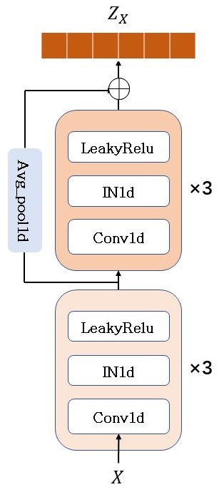
(a) Feature encoder

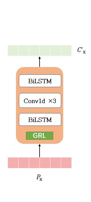
(b) Content predictor

Figure 2. Architecture of PMVC. $X$ means the mel-spectrograms of the input speech. $Z_{X}$ are the hidden feature representations, which contain the estimated content embeddings $C_{X}$ and estimated prosody embeddings $P_{X}$. 2 and 3 with multiplication symbol x denote the number of InstanceNorm1d and Conv1d layers.

As depicted in Figure 2, the design of the feature encoder is shown in Figure 2(a), which mainly draws on the content encoder of INVC (Chou and Lee, 2019). Different from (Chou and Lee, 2019), we drop the process of taking the concatenate between $X$ and hidden features as the final hidden feature $Z_{X}$. This ensures that $Z_{X}$ does not contain any timbre information. In addition, a leakyRelu function is introduced as the activation function. The architecture of the content predictor is shown in Figure 2(b), it uses two simple BiLSTM layers and three convolution layers to predict the estimated content embeddings according to the input prosody embedding. Besides, GRL is positioned between the feature encoder and the content predictor. Our decoder adopts the decoder of INVC as backbone. In the training process, the speaker embedding is duplicated to match the length of prosody and content embeddings. Then we concatenate them along the channel dimension which is then used as input of the decoder to reconstruct speech.

4. Experiments

In this section, we conduct comparative experiments for the evaluation of the proposed model’s performance on many-to-many VC and zero-shot VC tasks. As the traditional VC task, many-to-many VC means that in the inference phase select the speakers who have already appeared during training process as source and target. At the same time, zero-shot VC focuses on some more difficult tasks, in which the voice of both source speaker and target speaker are unseen during training. The audio demo is available on https://largeaudiomodel.com/pmvc/.

4.1. Datasets and Configurations

Table 1. Comparison of different models in traditional VC and zero-shot vc

Methods	Traditional VC				Zero-shot VC
	MCD	MOS	TSS	PSS	MCD	MOS	TSS	PSS
INVC	9.18 $\pm$ 0.34	2.95 $\pm$ 0.93	3.12 $\pm$ 0.77	2.74 $\pm$ 0.68	9.41 $\pm$ 0.58	2.75 $\pm$ 0.62	3.01 $\pm$ 0.89	2.66 $\pm$ 0.74
AutoVC	7.84 $\pm$ 0.17	3.24 $\pm$ 1.02	3.12 $\pm$ 0.86	2.87 $\pm$ 0.76	8.06 $\pm$ 0.39	3.11 $\pm$ 0.77	3.06 $\pm$ 0.93	2.59 $\pm$ 0.87
SpeechFlow	6.67 $\pm$ 0.29	3.49 $\pm$ 0.83	3.55 $\pm$ 0.69	3.39 $\pm$ 0.88	6.91 $\pm$ 0.43	3.51 $\pm$ 0.92	3.46 $\pm$ 0.87	3.33 $\pm$ 0.95
PMVC	6.06 $\pm$ 0.31	3.64 $\pm$ 0.90	3.91 $\pm$ 0.72	3.58 $\pm$ 0.84	5.98 $\pm$ 0.44	3.58 $\pm$ 0.73	3.85 $\pm$ 0.81	3.42 $\pm$ 0.77

Comparative experiments were conducted on the public corpus of AISHELL-3 (Shi et al., 2021). This corpus is a large-scale dataset including 88035 recordings from 218 native Chinese mandarin speakers, about 85 hours in total. In our experiments, all recordings have a sampling rate of 22.05kHz. We follow the same train/test partition and data preprocessing as (Tang et al., 2023d). Specially, We set the frame length of all training recordings to 256. That is, for any speech segments longer than 256, we randomly select 256 frames, at the same time, for those speech segments with a length shorter than 256, we pad them with constant. Besides, we divide the speech into multiple segments, each segment is 2 frames to achieve the Algorithm 1.

For the training of PMVC model, we set the batch size to 16 and the num of update steps is 400k. We use the ADAM optimizer (Kingma and Ba, 2015) ($\beta_{1}=0.9$, $\beta_{2}=0.99$, $\varepsilon=10^{-9}$). To obtain the speaker embedding, we select 10 utterances of the same speaker and feed them into the pretrained speaker encoder and then average the resulting embedding. We set the weights in Eq.(12) as follow: $\alpha=0.5,\beta=0.5$. Select AutoVC, INVC, and SpeechFlow models as baseline, following the training procedure in (Qian et al., 2019; Chou and Lee, 2019; Qian et al., 2020). Fairly, to get the result waveform, an pretrained Hifi-GAN (Kong et al., 2020) vocoder is used to convert the output mel-spectrogram.

4.2. Comparisons

Both objective and subjective experiments are conducted to compare different models’ performances in VC tasks. Detailly, the Mel-Cepstral Distortion (MCD) is adopted as an objective measure of the distance between the converted voice from source speaker and the real one from the target speaker.The lower MCD score means better performance.Moreover, 13 native speakers are invited as participants (nine males and four females) to do subjective tests for the quality assessment. The Mean Opinion Score (MOS) test needs every subject to choose a score on a scale from 1 to 5 for the naturalness of the converted speech after hearing them. The higher score indicates the opinion that the quality of hearing speech is better. Additionally, the Voice Similarity Score (VSS) test includes Timbre Similarity Score (TSS), and Prosody Similarity Score (PSS), where groups of utterances undergo voice similarity rating on a scale from 1 to 5. Each group contains four converted utterances from INVC, AutoVC, SpeechFlow, and PMVC, respectively, along with one real utterance of target speaker as reference. In the VSS test, higher score indicates the higher similarity between the converted result and ground truth speech.

As illustrated in Table 1, for the traditional many-to-many VC, 4 speakers are randomly selected from the training set (2 male and 2 female) and their utterances for the evaluation of multi many-to-many VC. Then test utterances of each of the 4 speakers are converted to the other 3 speakers respectively. This process generates a total of 4$\times$3 = 12 converted utterances each of which preserves the same linguistic information of speech from the 4 speakers speech but adopts the voice of the other 3 speakers. The MOS test results show that the converted speech from our model is of higher naturalness. The VSS test results show that our method surpasses INVC, AutoVC and SpeechSplit in learning better timbre and prosodic features for the converted speech, leading to an improvement in the overall conversion effect. Results of the objective and subjective tests demonstrate that compared with other baseline models, our PMVC performs better than other baseline models in VC tasks.

For the evaluation of zero-shot conversion, we select a few unseen speakers as the source and target speakers. To obtain their timbre embedding, take 10 utterances of the source and target speaker as the trained speaker encoder input, separately. As shown in Table 1, even on zero-shot condition, the proposed method still outperforms the baselines during naturalness evaluation. Moreover, compared to the synthesized results generated from baseline models, many people have the opinion that the converted results generated from our model sound more similar to the ground truth target, demonstrating PMVC’s efficiency in zero-shot VC.

4.3. Ablation Experiments

In this section, we first design an ablation experiment to observe the effect of $\mathcal{L}_{\text{adv}}$ on our framework. Specifically, we retrained our model without $\mathcal{L}_{\text{adv}}$ which we called ’PMVCs’. According to our assumption, without the constrain of the adversarial Mask-Predicted loss function, some content information may leak into the estimated prosody embeddings, and our model will eventually failed in the VC task. To test this hypothesis, we can leverage the trained content predictor in our model. Specifically, we randomly select 30 speeches (15 speeches selected from the training set, another 15 speeches belong to some unseen speaker.) as the input to get the estimated content embeddings and prosody embeddings of PMVC and PMVCs respectively. At the same time, based on these prosody embeddings, the pretrained content predictor will predict the estimated content embeddings. Obviously, the more accurate the prediction result is, the more overlapping information is contained in the estimated prosody embeddings and content embeddings.

Table 2. Results of the ablation experiments.

Method	Error (traditional-VC)	Error (zero-shot VC)
PMVC	0.76 $\pm$ 0.10	0.79 $\pm$ 0.14
PMVCs	0.14 $\pm$ 0.09	0.15 $\pm$ 0.11

The results summarized in Table 2 show that without $\mathcal{L}_{\text{adv}}$, the content predictor can easily output the content embeddings from the prosody embeddings, which indicates that the prosody embeddings contains almost all the information contained in the estimated content embeddings. At the same time, with the constrain of $\mathcal{L}_{\text{adv}}$, it will be difficult for the content predictor accurately predict the content embeddings from given prosody embeddings. In other words, our PMVC has a better performance than PMVCs in separating the content information and the prosodic information.

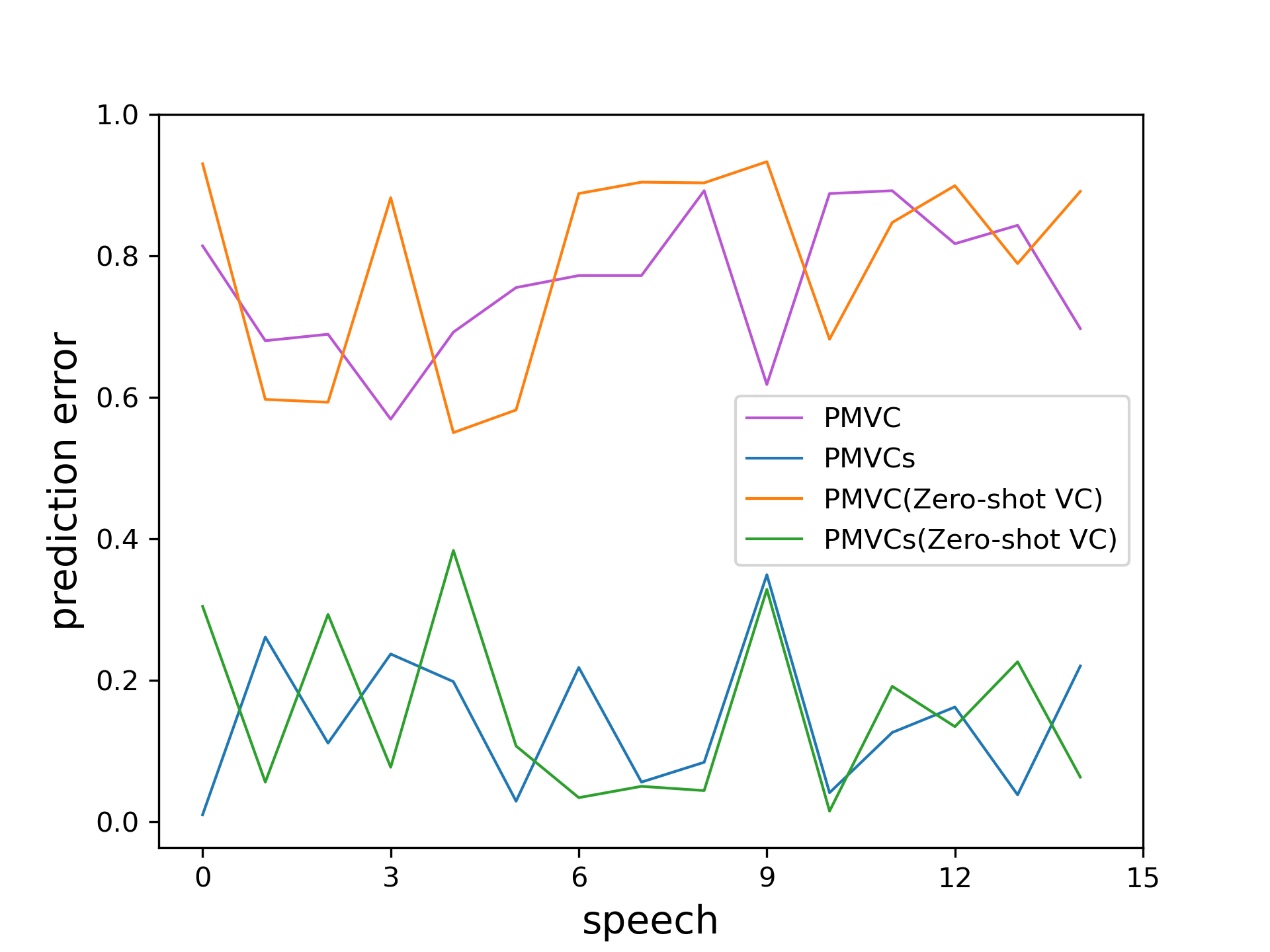
Figure 3. Prediction errors of PMVC and PMVCs on many-to-many VC tasks and zero-shot VC tasks.

As visual results shown in Figure 3, the prediction error scores show that under both many-to-many and zero-shot conditions, PMVC performs better than PMVCs in decoupling prosody and content information with higher scores. In addition, we can also find that the performance of PMVC is comparable under both conditions of one-shot VC and many-to-many VC, which indicates that our model can adapt well to new unseen speakers.

In addition, to further test the above hypothesis, we prepared the ground truth speech from the source speaker and target speaker respectively. We let the subjects listen to eight converted speeches produced by our model and the retrained model respectively. If the content information of a converted speech is recognized to belong to the target speaker, it indicates a successful VC task. Otherwise, the VC task is considered to have failed.

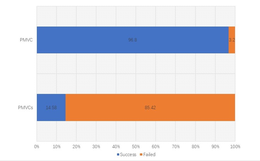
Figure 4. Subjective evaluation for the ablation experiments.

Results of the subjective evaluation (Figure 4) indicate that almost all subjects think the performance of the retrained model in VC task is very poor. At the same time, almost all subjects believe that the proposed PMVC have achieved the VC tasks. It indicates that the adversarial loss function is crucial for the proposed framework.

Furthermore, we also verified the feasibility of using only one encoder to extract the content embeddings and prosody embeddings by designing another set of comparative experiments. Specifically, we train a new model named PMVC_t, which mainly draws on PMVC, the only difference is that we add an additional prosody encoder to extract prosodic information in speech. And, the network structure design of the prosody encoder is almost exactly the same as our encoder. To regulate the dimension of the output feature, we simply add an linear layer at the end. To comprehensively compare PMVC and PMVC_t, we compare their performance and inference efficiency on the VC task, respectively.

Apart from MCD test mentioned above, we also add fake detection tests as another objective experiment, in which an open-source speech detection toolkit, Resemblyzer (https://github.com/resemble-ai/Resemblyzer) is utilized to compare how similar 7 unknown speeches to the ground truth reference audio(6 real ones, 2 fakes which are generated from PMVC and PMVC_t respectively). The converted speeches are divided into 20 groups for this test. Each group contains two converted utterances generated from PMVC and PMVC_t, respectively. The toolkit automatically assigns a score on a scale from 0 to 1 for each converted speech compared to reference audio which is ground truth. Higher score indicates that the converted speech has greater similarity to the target voice.

Table 3. Results of the ablation experiments.

Method	MCD Score	Detection Score	Model Size
PMVC	5.98 $\pm$ 0.44	0.73 $\pm$ 0.08	20.8M
PMVC_t	5.93 $\pm$ 0.35	0.70 $\pm$ 0.11	31.6M

As illustrated in Table 3, the results show that PMVC performs on par with PMVC_t on VC tasks. Specially, the MCD test result of PMVC_t is slightly better than that of PMVC, and the detection score of PMVC is slightly better than that of PMVC_t. However, the model size of PMVC is much smaller than PMVC_t, which means smaller parameters and faster training speed. All the above comparison results show that the proposed PMVC only using one encoder to extract content information and prosodic information can significantly improve the efficiency without reducing the quality of the converted speeches.

4.4. Flexible Hidden Features Dimensions

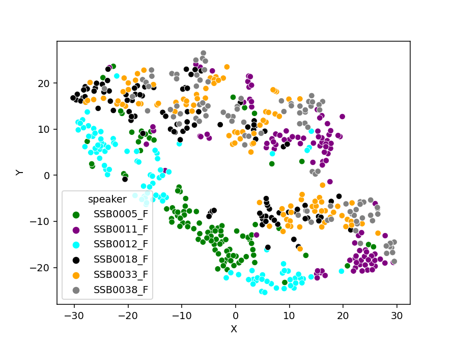
(a) Our model

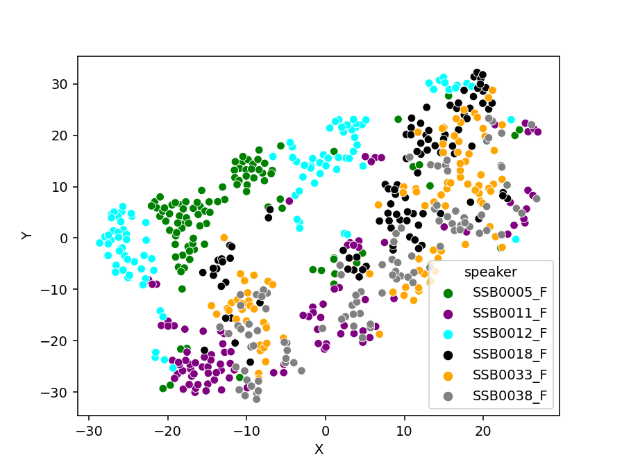
(b) M1

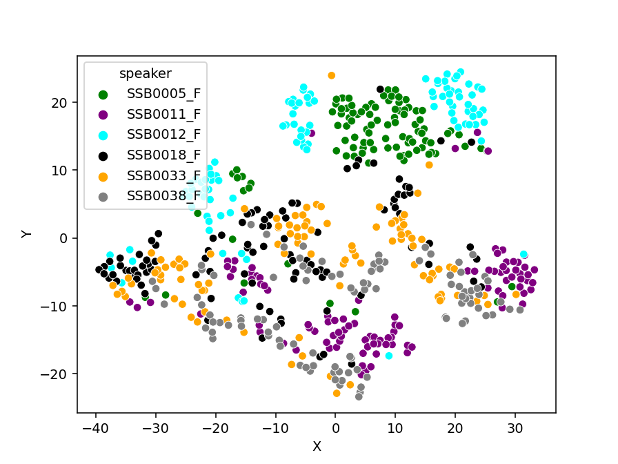
(c) M2

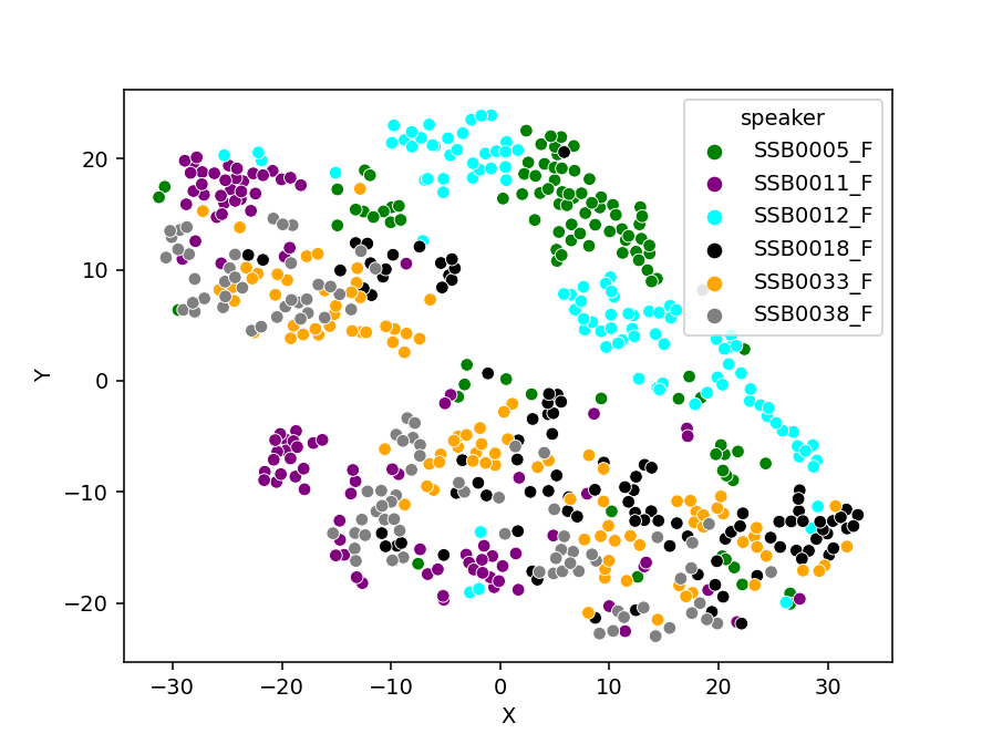
(d) M3

Figure 5. The visualization of hidden features.

In this section, we will discuss the strategy to divide the latent space $\boldsymbol{Z}$ into the content embedding $\boldsymbol{C_{x}}$ and prosody embedding $\boldsymbol{P_{x}}$. Selecting the right bottleneck size is crucial in AutoVC and SpeechSplit to preserve content information while excluding timbre details. But in our model, as we mentioned before, with the constrain of AdaIN and the loss function $\mathcal{L}_{\text{sim}}$ and $\mathcal{L}_{\text{recon}}$, even if we do not strictly limit the dimension of the feature embeddings, the $\boldsymbol{Z}$ tends to be split into two parts representing content and prosody information ideally. This enables us to easily determine the channel dimensions of $\boldsymbol{C_{x}}$ and $\boldsymbol{P_{x}}$ allowing for convenient extraction of both content embedding and prosody embedding using a single encoder.

To verify that the equivalent performance of the proposed model configured with different partition modes, we retrain the proposed model by modifying the length of dimensions of $\boldsymbol{C_{x}}$ and $\boldsymbol{P_{x}}$. Specifically, in the original model PMVC, both $\boldsymbol{C_{x}}$ and $\boldsymbol{P_{x}}$ have a channel-dimension of 128. Then, the model is retrained by changing their dimensions to 96 and 160, named ’M1’, or, to 64 and 192, named ’M2’. Also, we trained other models ’M3’ and ’M4’, which are set symmetric to ’M1’ and ’M2’. Specifically, in ’M3’, the dimensions of content and prosody embeddings are 160 and 96, and their dimensions change to 192 and 64 in ’M4’. Input the selected speakers’ utterances (100 utterances for each) to these models and derive the estimated hidden features $\boldsymbol{Z}$ ($\boldsymbol{C_{x}\oplus P_{x}}$), which then we visualize in 2D space using t-distributed stochastic neighbor embedding (t-SNE). As illustrated in Figure 5, it’s noted that the content and timbre information have evident separation regardless of the division proportion in the latent space.

The performance of these models under different partition modes were assessed in the VC task by exploiting the fake speech detection toolkit Resemblyzer again. Different from the above, in this time, each group contains five converted speeches generated from M1, M2, M3, M4 and our model, respectively. We present the result in Table 4.

Table 4. Comparison with retrained methods in VC tasks.

Method	Detection Score
PMVC ($\boldsymbol{C}$ : 128, $\boldsymbol{P}$ : 128)	0.74 $\pm$ 0.12
M1 ($\boldsymbol{C}$ : 96, $\boldsymbol{P}$ : 160)	0.72 $\pm$ 0.09
M2 ($\boldsymbol{C}$ : 64, $\boldsymbol{P}$ : 192)	0.75 $\pm$ 0.11
M3 ($\boldsymbol{C}$ : 160, $\boldsymbol{P}$ : 90)	0.74 $\pm$ 0.13
M4 ($\boldsymbol{C}$ : 192, $\boldsymbol{P}$ : 64)	0.72 $\pm$ 0.07

From Table 4, the results indicate that even under the changing division allocation of latent space, our model have equivalent performance in VC tasks. M2’s score seems to be slightly higher than others. We attribute this to the higher channel dimensions of the prosody embedding, enabling finer modeling of prosody details, which might influence the model’s VC performance.

Furthermore, we also try some subjective experiments for evaluation in VC task. In practice, 13 human participants are invited to hear a real speech and four converted speeches produced by our model and the retrained models respectively. They need to evaluate the similarity and select the converted speech which achieve the most similarity to the ground truth. Additionally, if it is difficult to judge, they can also choose the ’Fair’ option.

Figure 6. Subjective comparison of the converted speech.

Results shown in Figure 6 indicate that in VC task, the retrained model performs slightly worse than our proposed model, which further supports our hypothesis. That is, the performance of the proposed framework is compatible with different division modes.

5. Conclusion

In this paper, we propose a novel framework to address the problem of prosody modeling for expressive voice conversion. We firstly design a new random prosody algorithm to destroy the prosodic information of the source speech and obtain the corresponding augmented speech. Then, we extract and model the content, timbre, and prosodic features by using information-theory guided approaches. Both the subjective and objective experimental results demonstrate that the proposed method has made an improvement in both quality of the synthesized speech and improves its similarity to the target voice in VC tasks.

6. Acknowledgement

This paper is supported by the Key Research and Development Program of Guangdong Province under grant No.2021B0101400003. Corresponding author is Jianzong Wang from Ping An Technology (Shenzhen) Co., Ltd (jzwang@188.com).

References

- (1)
- Baevski et al. (2019) Alexei Baevski, Steffen Schneider, and Michael Auli. 2019. vq-wav2vec: Self-Supervised Learning of Discrete Speech Representations. In 8th International Conference on Learning Representations. OpenReview.net, Addis Ababa, Ethiopia, 1–12.
- Biadsy et al. (2019) Fadi Biadsy, Ron J. Weiss, Pedro J. Moreno, Dimitri Kanvesky, and Ye Jia. 2019. Parrotron: An End-to-End Speech-to-Speech Conversion Model and its Applications to Hearing-Impaired Speech and Speech Separation. In 20th Annual Conference of the International Speech Communication Association. ISCA, Graz, Austria, 4115–4119.
- Chou and Lee (2019) Ju-Chieh Chou and Hung-yi Lee. 2019. One-Shot Voice Conversion by Separating Speaker and Content Representations with Instance Normalization. In 20th Annual Conference of the International Speech Communication Association. ISCA, Graz, Austria, 664–668.
- Ding and Gutierrez-Osuna (2019) Shaojin Ding and Ricardo Gutierrez-Osuna. 2019. Group Latent Embedding for Vector Quantized Variational Autoencoder in Non-Parallel Voice Conversion. In 20th Annual Conference of the International Speech Communication Association. ISCA, Graz, Austria, 724–728.
- Gan et al. (2022) Wendong Gan, Bolong Wen, Ying Yan, Haitao Chen, Zhichao Wang, Hongqiang Du, Lei Xie, Kaixuan Guo, and Hai Li. 2022. IQDUBBING: Prosody modeling based on discrete self-supervised speech representation for expressive voice conversion. arXiv:2201.00269 00269, 2201 (2022), 1–5.
- Ganin and Lempitsky (2015) Yaroslav Ganin and Victor Lempitsky. 2015. Unsupervised domain adaptation by backpropagation. In Proceedings of the 32nd International Conference on Machine Learning. PMLR, JMLR.org, Lille, France, 1180–1189.
- Ghazvininejad et al. (2019) Marjan Ghazvininejad, Omer Levy, Yinhan Liu, and Luke Zettlemoyer. 2019. Mask-Predict: Parallel Decoding of Conditional Masked Language Models. In Proceedings of the 2019 Conference on Empirical Methods in Natural Language Processing and the 9th International Joint Conference on Natural Language Processing. Association for Computational Linguistics, Hong Kong, China, 6111–6120.
- Goodfellow et al. (2014) Ian Goodfellow, Jean Pouget-Abadie, Mehdi Mirza, Bing Xu, David Warde-Farley, Sherjil Ozair, Aaron Courville, and Yoshua Bengio. 2014. Generative adversarial nets. Advances in neural information processing systems 27 (2014), 1–5.
- Hsu et al. (2016) Chin-Cheng Hsu, Hsin-Te Hwang, Yi-Chiao Wu, Yu Tsao, and Hsin-Min Wang. 2016. Voice conversion from non-parallel corpora using variational auto-encoder. In 2016 Asia-Pacific Signal and Information Processing Association Annual Summit and Conference. IEEE, IEEE, Jeju, South Korea, 1–6.
- Kameoka et al. (2018) Hirokazu Kameoka, Takuhiro Kaneko, Kou Tanaka, and Nobukatsu Hojo. 2018. Stargan-vc: Non-parallel many-to-many voice conversion using star generative adversarial networks. In 2018 IEEE Spoken Language Technology Workshop. IEEE, IEEE, Athens, Greece, 266–273.
- Kaneko and Kameoka (2018) Takuhiro Kaneko and Hirokazu Kameoka. 2018. Cyclegan-vc: Non-parallel voice conversion using cycle-consistent adversarial networks. In 26th European Signal Processing Conference. IEEE, IEEE, Roma, Italy, 2100–2104.
- Kenter et al. (2019) Tom Kenter, Vincent Wan, Chun-an Chan, Rob Clark, and Jakub Vit. 2019. CHiVE: Varying Prosody in Speech Synthesis with a Linguistically Driven Dynamic Hierarchical Conditional Variational Network. In Proceedings of the 36th International Conference on Machine Learning, Vol. 97. PMLR, Long Beach, California, 3331–3340.
- Kingma and Ba (2015) Diederik P. Kingma and Jimmy Ba. 2015. Adam: A Method for Stochastic Optimization. In 3rd International Conference on Learning Representations. ICLR, San Diego, CA, USA, 1–5.
- Kong et al. (2020) Jungil Kong, Jaehyeon Kim, and Jaekyoung Bae. 2020. Hifi-gan: Generative adversarial networks for efficient and high fidelity speech synthesis. Advances in Neural Information Processing Systems 33 (2020), 17022–17033.
- Nguyen and Cardinaux (2022) Bac Nguyen and Fabien Cardinaux. 2022. Nvc-net: End-to-end adversarial voice conversion. In 2022 IEEE International Conference on Acoustics, Speech and Signal Processing. IEEE, IEEE, Virtual and Singapore, 7012–7016.
- Polyak and Wolf (2019a) Adam Polyak and Lior Wolf. 2019a. Attention-based Wavenet Autoencoder for Universal Voice Conversion. In 2019 IEEE International Conference on Acoustics, Speech and Signal Processing. IEEE, Brighton, United Kingdom, 6800–6804.
- Polyak and Wolf (2019b) Adam Polyak and Lior Wolf. 2019b. Attention-based Wavenet Autoencoder for Universal Voice Conversion. In 2019 IEEE International Conference on Acoustics, Speech and Signal Processing. IEEE, Brighton, United Kingdom, 6800–6804.
- Qian et al. (2020) Kaizhi Qian, Yang Zhang, Shiyu Chang, Mark Hasegawa-Johnson, and David Cox. 2020. Unsupervised speech decomposition via triple information bottleneck. In Proceedings of the 37th International Conference on Machine Learning. PMLR, PMLR, Virtual Event, 7836–7846.
- Qian et al. (2021) Kaizhi Qian, Yang Zhang, Shiyu Chang, Jinjun Xiong, Chuang Gan, David D. Cox, and Mark Hasegawa-Johnson. 2021. Global Rhythm Style Transfer Without Text Transcriptions. arXiv:2106.08519 08519, 2106 (2021), 1–5.
- Qian et al. (2019) Kaizhi Qian, Yang Zhang, Shiyu Chang, Xuesong Yang, and Mark Hasegawa-Johnson. 2019. Autovc: Zero-shot voice style transfer with only autoencoder loss. In Proceedings of the 36th International Conference on Machine Learning. PMLR, PMLR, Long Beach, California, 5210–5219.
- Shi et al. (2021) Yao Shi, Hui Bu, Xin Xu, Shaoji Zhang, and Ming Li. 2021. AISHELL-3: A Multi-Speaker Mandarin TTS Corpus. In 22nd Annual Conference of the International Speech Communication Association. ISCA, Incheon, Korea, 2756–2760.
- Skerry-Ryan et al. (2018) R. J. Skerry-Ryan, Eric Battenberg, Ying Xiao, Yuxuan Wang, Daisy Stanton, Joel Shor, Ron J. Weiss, Rob Clark, and Rif A. Saurous. 2018. Towards End-to-End Prosody Transfer for Expressive Speech Synthesis with Tacotron. In Proceedings of the 35th International Conference on Machine Learning, Vol. 80. PMLR, Stockholm, Sweden, 4700–4709.
- Stylianou et al. (1998) Yannis Stylianou, Olivier Cappé, and Eric Moulines. 1998. Continuous probabilistic transform for voice conversion. IEEE Transactions on speech and audio processing 6, 2 (1998), 131–142.
- Tang et al. (2022) Huaizhen Tang, Xulong Zhang, Jianzong Wang, Ning Cheng, and Jing Xiao. 2022. AVQVC: One-shot Voice Conversion by Vector Quantization with applying contrastive learning. In 2022 IEEE International Conference on Acoustics, Speech and Signal Processing. IEEE, IEEE, Virtual and Singapore, 4613–4617.
- Tang et al. (2023a) Haobin Tang, Xulong Zhang, Jianzong Wang, Ning Cheng, and Jing Xiao. 2023a. EmoMix: Emotion Mixing via Diffusion Models for Emotional Speech Synthesis. In 24th Annual Conference of the International Speech Communication Association. ISCA, Dublin, Ireland, 1–5.
- Tang et al. (2023b) Huaizhen Tang, Xulong Zhang, Jianzong Wang, Ning Cheng, and Jing Xiao. 2023b. Learning Speech Representations with Flexible Hidden Feature Dimensions. In 2023 IEEE International Conference on Acoustics, Speech and Signal Processing. IEEE, IEEE, Rhodes, Greek, 1–5.
- Tang et al. (2023c) Haobin Tang, Xulong Zhang, Jianzong Wang, Ning Cheng, and Jing Xiao. 2023c. QI-TTS: Questioning Intonation Control for Emotional Speech Synthesis. In 2023 IEEE International Conference on Acoustics, Speech and Signal Processing. IEEE, IEEE, Rhodes, Greek, 1–5.
- Tang et al. (2023d) Huaizhen Tang, Xulong Zhang, Jianzong Wang, Ning Cheng, and Jing Xiao. 2023d. VQ-CL: Learning Disentangled Speech Representations with Contrastive Learning and Vector Quantization. In 2023 IEEE International Conference on Acoustics, Speech and Signal Processing. IEEE, IEEE, Rhodes, Greek, 1–5.
- Tang et al. (2021) Huaizhen Tang, Xulong Zhang, Jianzong Wang, Ning Cheng, Zhen Zeng, Edward Xiao, and Jing Xiao. 2021. TGAVC: Improving Autoencoder Voice Conversion with Text-Guided and Adversarial Training. In 2021 IEEE Automatic Speech Recognition and Understanding Workshop. IEEE, IEEE, Cartagena, Colombia, 938–945.
- Ulyanov et al. (2016) Dmitry Ulyanov, Vadim Lebedev, Andrea Vedaldi, and Victor S. Lempitsky. 2016. Texture Networks: Feed-forward Synthesis of Textures and Stylized Images. In Proceedings of the 33nd International Conference on Machine Learning, Vol. 48. JMLR.org, New York City, NY, USA, 1349–1357.
- Valle et al. (2020) Rafael Valle, Jason Li, Ryan Prenger, and Bryan Catanzaro. 2020. Mellotron: Multispeaker Expressive Voice Synthesis by Conditioning on Rhythm, Pitch and Global Style Tokens. In 2020 IEEE International Conference on Acoustics, Speech and Signal Processing. IEEE, Barcelona, Spain, 6189–6193.
- Wan et al. (2018) Li Wan, Quan Wang, Alan Papir, and Ignacio Lopez Moreno. 2018. Generalized end-to-end loss for speaker verification. In 2018 IEEE International Conference on Acoustics, Speech and Signal Processing. IEEE, IEEE, Calgary, AB, Canada, 4879–4883.
- Wang et al. (2020) Jiashun Wang, Chao Wen, Yanwei Fu, Haitao Lin, Tianyun Zou, Xiangyang Xue, and Yinda Zhang. 2020. Neural Pose Transfer by Spatially Adaptive Instance Normalization. In 2020 IEEE/CVF Conference on Computer Vision and Pattern Recognition. Computer Vision Foundation / IEEE, Seattle, WA, USA, 5830–5838.
- Wang et al. (2018) Yuxuan Wang, Daisy Stanton, Yu Zhang, R. J. Skerry-Ryan, Eric Battenberg, Joel Shor, Ying Xiao, Ye Jia, Fei Ren, and Rif A. Saurous. 2018. Style Tokens: Unsupervised Style Modeling, Control and Transfer in End-to-End Speech Synthesis. In Proceedings of the 35th International Conference on Machine Learning (Proceedings of Machine Learning Research, Vol. 80). PMLR, Stockholm, Sweden, 5167–5176.
- Xie et al. (2021) Qicong Xie, Xiaohai Tian, Guanghou Liu, Kun Song, Lei Xie, Zhiyong Wu, Hai Li, Song Shi, Haizhou Li, Fen Hong, et al. 2021. The multi-speaker multi-style voice cloning challenge 2021. In 2021 IEEE International Conference on Acoustics, Speech and Signal Processing. IEEE, IEEE, Toronto, ON, Canada, 8613–8617.
- Zhou et al. (2021) Kun Zhou, Berrak Sisman, Rui Liu, and Haizhou Li. 2021. Seen and unseen emotional style transfer for voice conversion with a new emotional speech dataset. In 2021 IEEE International Conference on Acoustics, Speech and Signal Processing. IEEE, IEEE, Toronto, ON, Canada, 920–924.
- Zhou et al. (2022) Kun Zhou, Berrak Sisman, Rui Liu, and Haizhou Li. 2022. Emotional voice conversion: Theory, databases and ESD. Speech Communication 137 (2022), 1–18.